REVIEW OF EXPERIMENTAL DESIGN IN ANALYTICAL CHEMISTRY

www.iajpr.com

Pag

e55

0

Indo American Journal of Pharmaceutical Research, 2017 ISSN NO: 2231-6876

REVIEW OF EXPERIMENTAL DESIGN IN ANALYTICAL CHEMISTRY

T.Sudha*, G.Divya, J.Sujaritha,

P. Duraimurugan

Department of Pharmaceutical Analysis, Adhiparasakthi College of Pharmacy, Melmaruvathur-603 319.

Corresponding author

Dr. T. Sudha

M.Pharm, Ph.D,

Associate professor,

Department of Pharmaceutical Analysis,

Adhiparasakthi College of Pharmacy,

Melmaruvathur-603 319.

[email protected]

9362857380

Copy right © 2017 This is an Open Access article distributed under the terms of the Indo American journal of Pharmaceutical

Research, which permits unrestricted use, distribution, and reproduction in any medium, provided the original work is properly cited.

ARTICLE INFO ABSTRACT

Article history

Received 01/08/2017

Available online

31/08/2017

Keywords

Experimental Design,

Response Surface

Methodology,

Factorial Design,

Optimization,

Fractional Factorial Design.

The ability of a chromatographic method to successfully separate, identify and quantitative

species is determined by many factors, many of which are in the control of the experimenter.

When attempting to discover the important factors and then optimize a response by turning

these factors by using multivariate statistical techniques for the optimization of

chromatographic system. The surface response methodologies and experimental design give a

powerful suite of statistical methodology. Advantage includes modeling by empherical

function, a defined number of experiments to be performed and available software to

accomplish the task of two uses of experimental design in chromatography for showing lack

of significant factors and then optimizing a response within their method development.

Plackett - Burman design (Screening) widely used in validation studies and fraction factorial

designs and their extensions such as (response surface) central composite designs are most

popular optimizers. Box-Behnken and Doehlert designs are becoming more used as efficient

alternatives. The use of mixture designs for optimization of mobile phase is also related. A

discussion about model validation is presented. Then simultaneously the multiple responses

are optimized, the desirability function is used and discussed the criteria for judging the

quality of a chromatogram by using multi criteria decision making studies. Some applications

of multivariate techniques for optimization of chromatographic methods are also summarized.

Please cite this article in press as Dr. T. Sudha et al. Review of Experimental Design in Analytical Chemistry. Indo American

Journal of Pharmaceutical Research.2017:7(08).

mailto:[email protected]

www.iajpr.com

Pag

e55

1

Vol 7, Issue 08, 2017. Dr. T. Sudha et al. ISSN NO: 2231-6876

Selection of important factors

INTRODUCTION

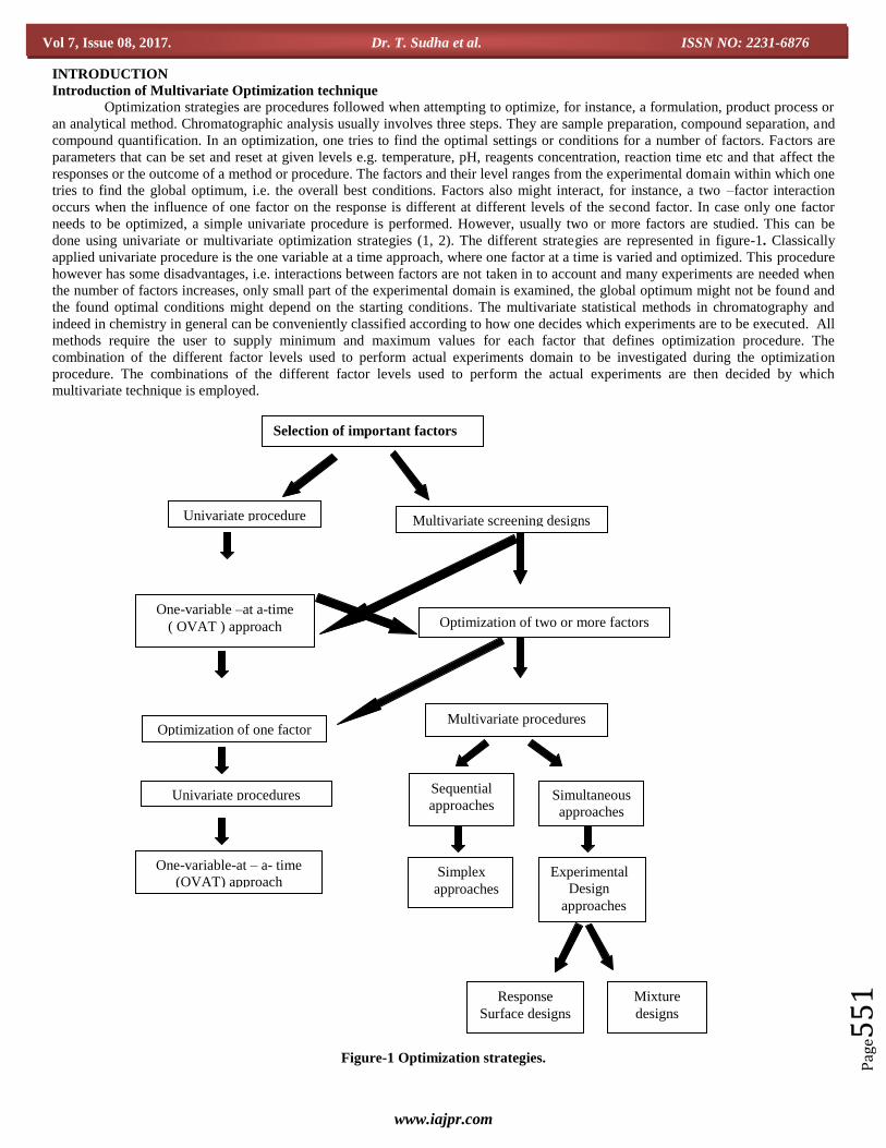
Introduction of Multivariate Optimization technique Optimization strategies are procedures followed when attempting to optimize, for instance, a formulation, product process or

an analytical method. Chromatographic analysis usually involves three steps. They are sample preparation, compound separation, and

compound quantification. In an optimization, one tries to find the optimal settings or conditions for a number of factors. Factors are

parameters that can be set and reset at given levels e.g. temperature, pH, reagents concentration, reaction time etc and that affect the

responses or the outcome of a method or procedure. The factors and their level ranges from the experimental domain within which one

tries to find the global optimum, i.e. the overall best conditions. Factors also might interact, for instance, a two –factor interaction

occurs when the influence of one factor on the response is different at different levels of the second factor. In case only one factor

needs to be optimized, a simple univariate procedure is performed. However, usually two or more factors are studied. This can be

done using univariate or multivariate optimization strategies (1, 2). The different strategies are represented in figure-1. Classically

applied univariate procedure is the one variable at a time approach, where one factor at a time is varied and optimized. This procedure

however has some disadvantages, i.e. interactions between factors are not taken in to account and many experiments are needed when

the number of factors increases, only small part of the experimental domain is examined, the global optimum might not be found and

the found optimal conditions might depend on the starting conditions. The multivariate statistical methods in chromatography and

indeed in chemistry in general can be conveniently classified according to how one decides which experiments are to be executed. All

methods require the user to supply minimum and maximum values for each factor that defines optimization procedure. The

combination of the different factor levels used to perform actual experiments domain to be investigated during the optimization

procedure. The combinations of the different factor levels used to perform the actual experiments are then decided by which

multivariate technique is employed.

Figure-1 Optimization strategies.

Multivariate screening designs Univariate procedure

Optimization of two or more factors One-variable –at a-time

( OVAT ) approach

Multivariate procedures Optimization of one factor

Sequential

approaches

Simplex

approaches

Simultaneous

approaches

Experimental

Design

approaches

Mixture

designs

Response

Surface designs

Univariate procedures

One-variable-at – a- time

(OVAT) approach

www.iajpr.com

Pag

e55

2


Terminology of Design of experiments

The definitions below are given in the style of the international Vocabulary of Metrology (VIM), where definitions of basic

concepts in measurement are found [3].

Experimental design:

Statistical technique for planning, conducting, analyzing and interpreting data from experiments.

Response: Measured or observed quantity that is the subject of study or optimization.

Example: Chromatographic response factor, retention factor and number of theoretical plates.

Factor: Quantity that affects the response

1. Factors are considered as controlled or uncontrolled depending on whether the levels of the factor can be set in the experimental

design.

2. Factors can take discrete or continuous values. Eg: Column temperature, concentration of organic phase.

3. Synonyms are variable, predictor and parameter.

Level of a factor:

Value of a factor that is prescribed in an experimental design.

Response surface: Relationship of a response to values of one or more factors.

1. The surface is usually a plot in two or three dimensions of the functions that is fitted to the experimental data.

2. Response surface methodology is used to describe the use of experimental designs that give response surfaces from which

information about the system is deduced [4].

Model: Equation that relates a response to factors. A model can be empirical, which is chosen for the mathematical form, or is based

on a theoretical understanding of the process that gives the response. Empirical model based on polynomials of the factors are

described by the order of the polynomial. eg. I order and II order.

Effect:

Co-efficient of a term in a model. The main effect is the co-efficient of the term in the first order of a factor. Interaction

effects are co-efficient of products of linear terms. eg: two-way interaction, three –way interactions.

Factorial designs:

Experimental design in which the runs are combination of levels of factors.

1. Full factorial designs have every possible combination of factors at the designated levels. There are LK combinations of K factors

at L levels.

2. Fractional factorial designs are a specific subset of a full design.

3. Other experimental design includes Plackett- Burman, Central composite design, Box-Behnken, Doehlert, D-optimal, G-optimal

and mixture design.

Optimization Strategies

In any modeling and optimization exercise there is an initial decision to be made between empirical approaches and ones that

use scientific knowledge about the system under study [5].Calculated mobility co-efficient were fitted to observations with

equilibrium constant as factors. The availability of credible theoretical models should always be considered. However in the case

where such theoretical modeling is not feasible or is overkill in a system that simply requires optimizing, design of experiment has the

advantage of providing recipes of experiments that are independent of the system itself. Experimental design also has the advantage

over iterative estimators such as simplex that the number of experiments is determined before any work is done. Assuming the factors,

factor levels are chosen appropriately. Then the outcome is assumed with a known effort. This advantage is particularly useful in

modern system with fully programmable system with auto samples in which a run can be set up in the evening and the results

available in the morning.

Kinds of problems informed by experimental design

There are two kinds of chemical problems that need experimental design for their solution.

1. To discover which factor may significantly affect the response of the experiment

2. To find factor values that optimizes the response.

www.iajpr.com

Pag

e55

3


Choice of Response Chromatography is full of trade –offs and an optimum separation depends on the wider problems with considerations such as

time, cost required measurement uncertainty, that is the use to which the analytical information is to be put. Advantages of design of

experiment are that multiple responses can be measured (resolution, time, throughput) and models developed that arrive at the desired

over all optimum without extra experiments.

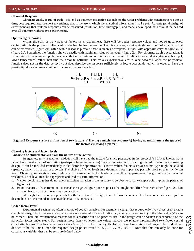
Optimizing responses Within the span of the values of factors in an experiment, there will be better response values and not so good ones.

Optimization is the process of discovering whether the best values lie. Then is not always a nice single maximum of a function that

can be discovered (figure-2a). Often within response plateaus there is an area of response surface with approximately the same value

(figure-2c). Sometimes the function shows a saddle with maximum value of the edges (figure-2b). For chromatographic separations it

is important to have an acceptable response that meets minimum criteria and so the aim is often to locate that region (eg: high pH,

lower temperature) rather than find the absolute optimum. This makes experimental design very powerful when the polynomial

function does not fit the data perfectly but does describe the response sufficiently to locate acceptable region. In order to have the

possibility of maximum or minimum quadratic terms are needed.

i=k i=kj-k-1 i=k

R= β0 +∑ βixi + ∑ ∑ βijxixj +∑βiixi2 + ε

i-1 i=1 j-i

(a) (b) (c)

Figure-2 Response surface as function of two factors a) Having a maximum response b) having no maximum in the space of

the factors c) Having a plateau.

Choosing factors and factor levels

Factors to be studied obvious from the nature of the system.

Ruggedness tests in method validation will have had the factors for study prescribed in the protocol [6]. If it is known that a

factor has a great effect of separation (perhaps column temperature) there is no point in discovering this information in a screening

design. It can be included immediately in the factor for optimization. Discrete valued factors such as column type might be studied

separately rather than a part of a design. The choice of factor levels in a design is most important; possibly more so than the design

itself. Obtaining information using only a small number of factor levels is strength of experimental design but also a potential

weakness. Each level must be appropriate and lead to useful information.

1. Values too close together do not allow sufficient variation in the response to be observed. (for example points up on the plateau of

figure-2c).

2. Points that are at the extreme of a reasonable range will give poor responses that might not differ from each other figure -2a. Not

all combination of factor levels may be practical.

Although the researchers proceeded with the rest of the design, it would have been better to choose other values or go to a

design than can accommodate inaccessible areas of factor space.

Coded factor levels Experimental designs are often in terms of coded variables. For example a design that require only two values of a variable

(two level design) factor values are usually given as a series of +1 and -1 indicating whether one value (+1) or the other value (-1) is to

be chosen. There are mathematical reasons for this practice but also practical use in the design can be written independently of the

particular factor under study. For designs more than two levels, the values indicate the relative circumscribed two factor central

composite designs. The five coded levels are -√2, -1, 0, +1, +√2. For eg: the factors were temperature and range to be studied was

decided to be 50-100º C then the required design points would be 50, 57, 75, 93, 100 ºC. Note that this can only be done for

continuous variables that can be set a predefined value.

www.iajpr.com

Pag

e55

4


Kinds of experimental Designs

There are many different kinds of design. They can be distinguished by the model that is desired (Linear or Quadratic, with

or without interaction) constraints on factor levels, and the purpose of the study (Screening, Optimization). Many designs (orthogonal

design) vary the factors independently of each other which eliminate correlations among the factors.

Factorial Designs

Factorial designs identify experiments at every combination of factor levels. There are LK combinations of ‘L’-levels of ‘K’-

factors. In full factorial designs every experiment is performed, while the fractional factorial design as specific subset is performed

that allows calculation of certain co-efficient of the model. Two level designs are chosen for screening factors and can give main and

interaction effects, but not higher order. Fractionation leads to design that give main effects only with fewer runs. Calculation of

effects in two level designs is easy and can be performed in a spread sheet. If the two levels are coded +1 and -1, then the column of

+1 and -1 under each factor is multiplied by the response for each experiment. The product is summed and divided by half the number

of experiments. This is the main effect for the factor. For an interaction effect a column is created that is the product of the level codes

and the procedure outlined above is applied to this column.

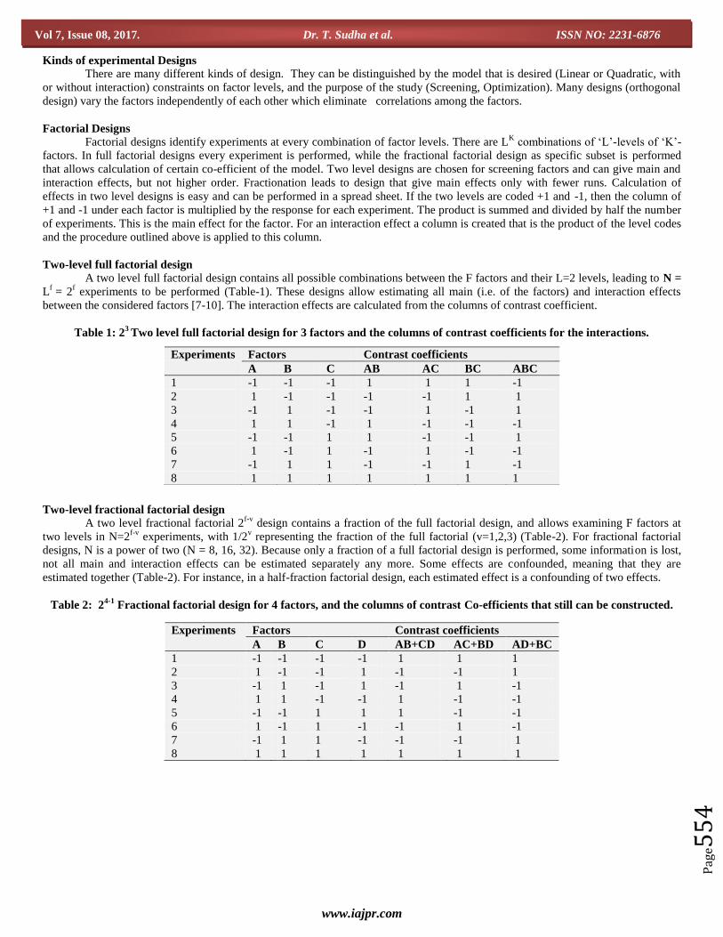
Two-level full factorial design

A two level full factorial design contains all possible combinations between the F factors and their L=2 levels, leading to N =

Lf = 2

f experiments to be performed (Table-1). These designs allow estimating all main (i.e. of the factors) and interaction effects

between the considered factors [7-10]. The interaction effects are calculated from the columns of contrast coefficient.

Table 1: 23 Two level full factorial design for 3 factors and the columns of contrast coefficients for the interactions.

Two-level fractional factorial design

A two level fractional factorial 2f-v

design contains a fraction of the full factorial design, and allows examining F factors at

two levels in N=2f-v

experiments, with 1/2v representing the fraction of the full factorial (v=1,2,3) (Table-2). For fractional factorial

designs, N is a power of two (N = 8, 16, 32). Because only a fraction of a full factorial design is performed, some information is lost,

not all main and interaction effects can be estimated separately any more. Some effects are confounded, meaning that they are

estimated together (Table-2). For instance, in a half-fraction factorial design, each estimated effect is a confounding of two effects.

Table 2: 24-1

Fractional factorial design for 4 factors, and the columns of contrast Co-efficients that still can be constructed.

Experiments Factors Contrast coefficients

A B C AB AC BC ABC

1 -1 -1 -1 1 1 1 -1

2 1 -1 -1 -1 -1 1 1

3 -1 1 -1 -1 1 -1 1

4 1 1 -1 1 -1 -1 -1

5 -1 -1 1 1 -1 -1 1

6 1 -1 1 -1 1 -1 -1

7 -1 1 1 -1 -1 1 -1

8 1 1 1 1 1 1 1

Experiments Factors Contrast coefficients

A B C D AB+CD AC+BD AD+BC

1 -1 -1 -1 -1 1 1 1

2 1 -1 -1 1 -1 -1 1

3 -1 1 -1 1 -1 1 -1

4 1 1 -1 -1 1 -1 -1

5 -1 -1 1 1 1 -1 -1

6 1 -1 1 -1 -1 1 -1

7 -1 1 1 -1 -1 -1 1

8 1 1 1 1 1 1 1

www.iajpr.com

Pag

e55

5


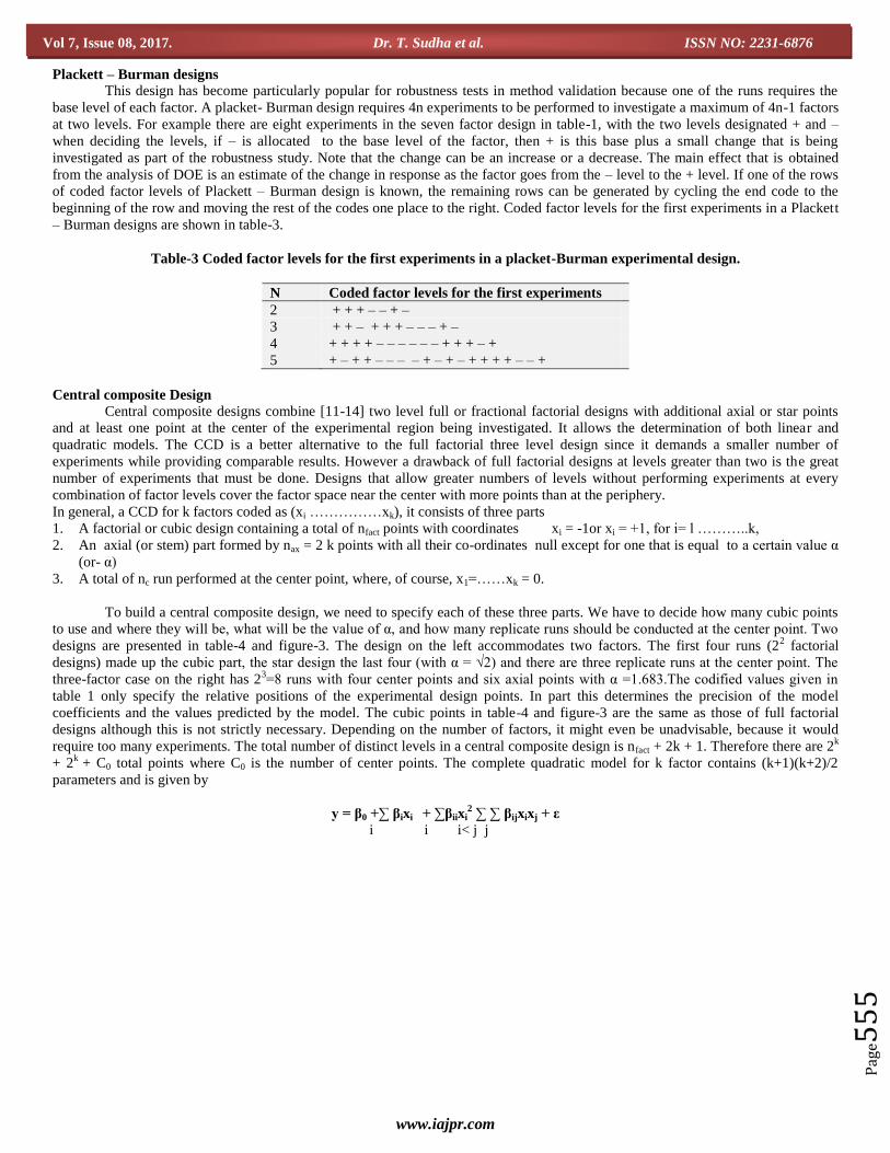
Plackett – Burman designs

This design has become particularly popular for robustness tests in method validation because one of the runs requires the

base level of each factor. A placket- Burman design requires 4n experiments to be performed to investigate a maximum of 4n-1 factors

at two levels. For example there are eight experiments in the seven factor design in table-1, with the two levels designated + and –

when deciding the levels, if – is allocated to the base level of the factor, then + is this base plus a small change that is being

investigated as part of the robustness study. Note that the change can be an increase or a decrease. The main effect that is obtained

from the analysis of DOE is an estimate of the change in response as the factor goes from the – level to the + level. If one of the rows

of coded factor levels of Plackett – Burman design is known, the remaining rows can be generated by cycling the end code to the

beginning of the row and moving the rest of the codes one place to the right. Coded factor levels for the first experiments in a Plackett

– Burman designs are shown in table-3.

Table-3 Coded factor levels for the first experiments in a placket-Burman experimental design.

N Coded factor levels for the first experiments

2 + + + – – + –

3 + + – + + + – – – + –

4 + + + + – – – – – – + + + – +

5 + – + + – – – – + – + – + + + + – – +

Central composite Design

Central composite designs combine [11-14] two level full or fractional factorial designs with additional axial or star points

and at least one point at the center of the experimental region being investigated. It allows the determination of both linear and

quadratic models. The CCD is a better alternative to the full factorial three level design since it demands a smaller number of

experiments while providing comparable results. However a drawback of full factorial designs at levels greater than two is the great

number of experiments that must be done. Designs that allow greater numbers of levels without performing experiments at every

combination of factor levels cover the factor space near the center with more points than at the periphery.

In general, a CCD for k factors coded as (xi ……………xk), it consists of three parts

1. A factorial or cubic design containing a total of nfact points with coordinates xi = -1or xi = +1, for i= l ………..k,

2. An axial (or stem) part formed by nax = 2 k points with all their co-ordinates null except for one that is equal to a certain value α

(or- α)

3. A total of nc run performed at the center point, where, of course, x1=……xk = 0.

To build a central composite design, we need to specify each of these three parts. We have to decide how many cubic points

to use and where they will be, what will be the value of α, and how many replicate runs should be conducted at the center point. Two

designs are presented in table-4 and figure-3. The design on the left accommodates two factors. The first four runs (22 factorial

designs) made up the cubic part, the star design the last four (with α = √2) and there are three replicate runs at the center point. The

three-factor case on the right has 23=8 runs with four center points and six axial points with α =1.683.The codified values given in

table 1 only specify the relative positions of the experimental design points. In part this determines the precision of the model

coefficients and the values predicted by the model. The cubic points in table-4 and figure-3 are the same as those of full factorial

designs although this is not strictly necessary. Depending on the number of factors, it might even be unadvisable, because it would

require too many experiments. The total number of distinct levels in a central composite design is nfact + 2k + 1. Therefore there are 2k

+ 2k

+ C0 total points where C0 is the number of center points. The complete quadratic model for k factor contains (k+1)(k+2)/2

parameters and is given by

y = β0 +∑ βixi + ∑βiixi2 ∑ ∑ βijxixj + ε

i i i< j j

www.iajpr.com

Pag

e55

6


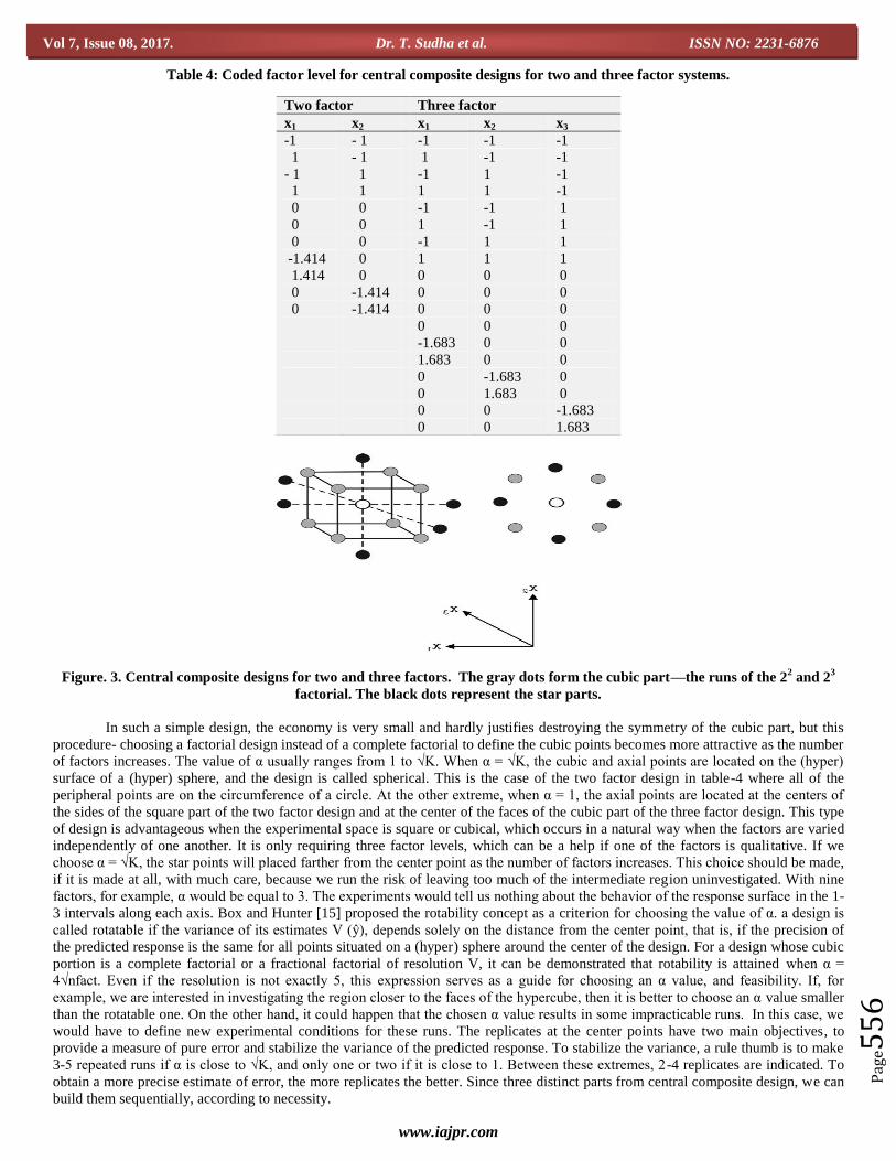
Table 4: Coded factor level for central composite designs for two and three factor systems.

Figure. 3. Central composite designs for two and three factors. The gray dots form the cubic part—the runs of the 22 and 2

3

factorial. The black dots represent the star parts.

In such a simple design, the economy is very small and hardly justifies destroying the symmetry of the cubic part, but this

procedure- choosing a factorial design instead of a complete factorial to define the cubic points becomes more attractive as the number

of factors increases. The value of α usually ranges from 1 to √K. When α = √K, the cubic and axial points are located on the (hyper)

surface of a (hyper) sphere, and the design is called spherical. This is the case of the two factor design in table-4 where all of the

peripheral points are on the circumference of a circle. At the other extreme, when α = 1, the axial points are located at the centers of

the sides of the square part of the two factor design and at the center of the faces of the cubic part of the three factor design. This type

of design is advantageous when the experimental space is square or cubical, which occurs in a natural way when the factors are varied

independently of one another. It is only requiring three factor levels, which can be a help if one of the factors is qualitative. If we

choose α = √K, the star points will placed farther from the center point as the number of factors increases. This choice should be made,

if it is made at all, with much care, because we run the risk of leaving too much of the intermediate region uninvestigated. With nine

factors, for example, α would be equal to 3. The experiments would tell us nothing about the behavior of the response surface in the 1-

3 intervals along each axis. Box and Hunter [15] proposed the rotability concept as a criterion for choosing the value of α. a design is

called rotatable if the variance of its estimates V (ŷ), depends solely on the distance from the center point, that is, if the precision of

the predicted response is the same for all points situated on a (hyper) sphere around the center of the design. For a design whose cubic

portion is a complete factorial or a fractional factorial of resolution V, it can be demonstrated that rotability is attained when α =

4√nfact. Even if the resolution is not exactly 5, this expression serves as a guide for choosing an α value, and feasibility. If, for

example, we are interested in investigating the region closer to the faces of the hypercube, then it is better to choose an α value smaller

than the rotatable one. On the other hand, it could happen that the chosen α value results in some impracticable runs. In this case, we

would have to define new experimental conditions for these runs. The replicates at the center points have two main objectives, to

provide a measure of pure error and stabilize the variance of the predicted response. To stabilize the variance, a rule thumb is to make

3-5 repeated runs if α is close to √K, and only one or two if it is close to 1. Between these extremes, 2-4 replicates are indicated. To

obtain a more precise estimate of error, the more replicates the better. Since three distinct parts from central composite design, we can

build them sequentially, according to necessity.

Two factor Three factor

x1 x2 x1 x2 x3

-1 - 1 -1 -1 -1

1 - 1 1 -1 -1

- 1 1 -1 1 -1

1 1 1 1 -1

0 0 -1 -1 1

0 0 1 -1 1

0 0 -1 1 1

-1.414 0 1 1 1

1.414 0 0 0 0

0 -1.414 0 0 0

0 -1.414 0 0 0

0 0 0

-1.683 0 0

1.683 0 0

0 -1.683 0

0 1.683 0

0 0 -1.683

0 0 1.683

www.iajpr.com

Pag

e55

7


If we happen to be in a region of the response surface where curvature is not important, there is no need fit a quadratic model.

The cubic part of the design is sufficient for fitting a linear model, from which we can rapidly move to a more interesting region

extending the investigation. Even if we are in doubt about possible curvature, we can test its significance using the runs at the center

point. Then, if the curvature is found significant, we can complete the design with the axial points. Actually we would be performing

the runs of the complete design in two blocks - first the cubic and then the axial one. Suppose that the response values in the axial

block contain a systematic error in relation to the response values obtained in the first block. Under certain conditions, this error will

not affect the coefficient estimates for the model, that is, the block effect will not confound itself with the effects of the factors. This

will occur if the design blocking is orthogonal, which in turn depends on the α value. Blocking will be orthogonal if:

α = √nfact (nax + nc, ax)

2(nfact + nc, fact)

nc, fact and nc,ax are the number of runs at the center point in the cubic and blocks, respectively.

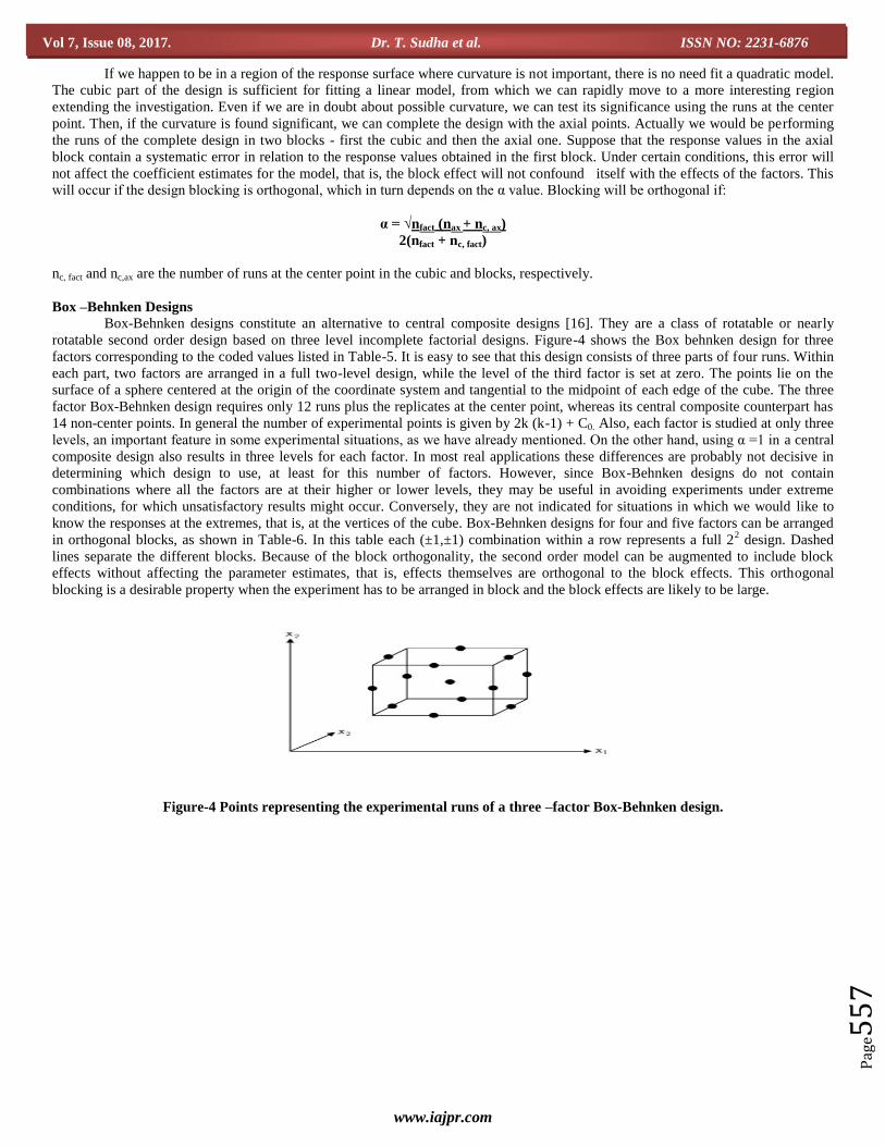
Box –Behnken Designs Box-Behnken designs constitute an alternative to central composite designs [16]. They are a class of rotatable or nearly

rotatable second order design based on three level incomplete factorial designs. Figure-4 shows the Box behnken design for three

factors corresponding to the coded values listed in Table-5. It is easy to see that this design consists of three parts of four runs. Within

each part, two factors are arranged in a full two-level design, while the level of the third factor is set at zero. The points lie on the

surface of a sphere centered at the origin of the coordinate system and tangential to the midpoint of each edge of the cube. The three

factor Box-Behnken design requires only 12 runs plus the replicates at the center point, whereas its central composite counterpart has

14 non-center points. In general the number of experimental points is given by 2k (k-1) + C0. Also, each factor is studied at only three

levels, an important feature in some experimental situations, as we have already mentioned. On the other hand, using α =1 in a central

composite design also results in three levels for each factor. In most real applications these differences are probably not decisive in

determining which design to use, at least for this number of factors. However, since Box-Behnken designs do not contain

combinations where all the factors are at their higher or lower levels, they may be useful in avoiding experiments under extreme

conditions, for which unsatisfactory results might occur. Conversely, they are not indicated for situations in which we would like to

know the responses at the extremes, that is, at the vertices of the cube. Box-Behnken designs for four and five factors can be arranged

in orthogonal blocks, as shown in Table-6. In this table each (±1,±1) combination within a row represents a full 22 design. Dashed

lines separate the different blocks. Because of the block orthogonality, the second order model can be augmented to include block

effects without affecting the parameter estimates, that is, effects themselves are orthogonal to the block effects. This orthogonal

blocking is a desirable property when the experiment has to be arranged in block and the block effects are likely to be large.

Figure-4 Points representing the experimental runs of a three –factor Box-Behnken design.

www.iajpr.com

Pag

e55

8


Table 5: Coded factor levels for a Box – Behnken design for a three –variable system.

x1 x2 x3

-1 -1 0

1 -1 0

-1 1 0

1 1 0

-1 0 -1

1 0 -1

-1 0 1

1 0 1

0 -1 -1

0 1 -1

0 -1 1

0 1 1

0 0 0

0 0 0

0 0 0

0 0 0

Table 6: Coded factor levels for Box-Behnken designs for four and five factors.

Four-factor Five-factor

x1 x2 x3 x4 x1 x2 x3 x4 x5

±1

0

0

±1

0

0

0

±1

0

0

±1

0

±1

0

0

±1

0

0

±1

0

±1

0

0

0

0

±1

0

±1

0

0

0

±1

0

0

±1

0

0

0

±1

0

±1

0 ±1

0

0

0

±1

0

0

±1

0

±1

0

0 0

±1

0

±1

0

0

±1

0

0

0

±1

0

±1

0

±1

0

0

0

0

±1

0

0

±1

0

0

0

±1

±1

0

0

±1

0

0

0

±1

0

±1

0

0

0

±1

0

Doehlert designs Doehlert designs, unlike central composite and Box-Behnken are not rotatable, i.e. they can give different qualities of

estimates for different factors. However, it is advantageous to use design where different factors are studied at different number of

levels. Thus factors that are considered more important can be measured at more levels. They are attractive for treating problems

where specific information about the system indicates that some factors deserve more attention than others, but they also have other

desirable characteristics. All Doehlert designs are generated from a regular simplex, a geometrical figure containing k+1 points, where

k is the number of factors. For two factors, the regular simplex is an equilateral triangle. For Doehlert designs of type D-1, which are

the most popular, the coordinates of this triangle are those given in the first three lines of table-7 in coded units. The other runs of the

design are obtained by subtracting every run in the triangle from each other, as shown in the table. This corresponds to moving the

simplex around the design center. For any number of factors k, one of the points of the simplex is the origin, and the other k points lie

on the surface of a sphere with radius 1.0 centered on the origin, in such a way that the distances between neighboring points are all

the same. Each of these points subtracted from the other k points forms k new points, so the design matrix has a total of k2

+ k + 1

points. Since the points are uniformly distributed on a spherical shell, Doehlert [17] suggested that these designs can be called uniform

shell designs. The coordinates of the D-1 designs for three and four factors are presented in table-8. Note that the design for k=3 is the

same as the corresponding Box-Behnken design. Compared to central composite or Box – Behnken designs, Doehlert designs are

more economical, especially as the number of factors increase. The basic hexagon in figure-5 has six points lying on a circumference

around the center point, whereas the two factor central composite design has eight points, also lying on a circumference surrounding

its center point. Likewise, the three factor Doehlert design has 13 points, but the central composite design requires 15. On the other

hand, central composite designs are rotatable, a general property that Doehlert designs do not have. Furthermore, since central

composite designs consist of factorial and axial blocks, they provide the basis for an efficient sequential strategy. Linear models can

be fitted in a first stage, after which the designs can be augmented with complementary points, should quadratic models prove

necessary.

www.iajpr.com

Pag

e55

9


Finally, using full designs, Doehlert or otherwise, to fit second order models is hardly practicable for more than four factors,

since a five factor quadratic model has twenty coefficients to be determined and it is unlikely that all factor will be relevant.

Fractional; factorial screening design to discriminate between inert and relevant factors should always be applied before higher order

designs when many factors are being investigated. Another very interesting feature of Doehlert designs is the possibility of

introducing variations in new factors during the course of an experimental study, without losing the runs already performed.

Sometimes we might wish to study first say the two factors that seem more promising, analyze the results, and only then introduce

variation in a third factor, then in fourth, and so on. With Doehlert D-1 designs this is possible, provided that all potential factors of

interest are introduced in the experiments right from start, set at their average levels (that is, zero in coded units). As can see in Table -

8 , a Doehlert design of type D-1 with three or more factors always has one factor at five levels (the first one), one factor at three

levels ( the last), and the others all at seven levels. Two other Doehlert design types, D-2 and D-3 can be generated by different

simplexes and result in different level distributions.

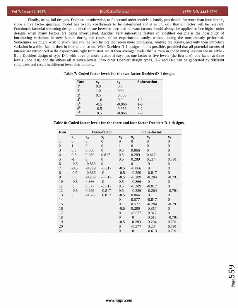
Table 7: Coded factor levels for the two-factor DoehlertD-1 design.

Table 8: Coded factor levels for the three and four factor Doehlert D-1 designs.

Run x1 x2 Subtraction

1a 0.0 0.0

2a 1.0 000

3a 0.5 0.866

4b -1.0 0.0 1-2

5b -0.5 -0.866 1-3

6b -0.5 0.866 3-2

7b 0.5 -0.866 2-3

Run Three-factor Four-factor

x1 x2 x3 x1 x2 x3 x4

1 0 0 0 0 0 0 0

2 1 0 0 1 0 0 0

3 0.5 0.866 0 0.5 0.866 0 0

4 0.5 0.289 0.817 0.5 0.289 0.817 0

5 -1 0 0 0.5 0.289 0.214 0.791

6 -0.5 -0.866 0 -1 0 0 0

7 -0.5 -0.289 -0.817 -0.5 -0.866 0 0

8 0.5 -0.866 0 -0.5 -0.289 -0.817 0

9 0.5 -0.289 -0.817 -0.5 -0,289 -0.204 -0.791

10 -0.5 0.866 0 0.5 -0.866 0 0

11 0 0.577 -0.817 0.5 -0.289 -0.817 0

12 -0.5 0.289 0.817 0.5 -0.289 -0.204 -0.791

13 0 -0.577 0.817 -0.5 0.866 0 0

14 0 0.577 -0.817 0

15 0 0.577 -0.204 -0.791

16 -0.5 0.289 0.817 0

17 0 -0.577 0.817 0

18 0 0 0.613 -0.791

19 -0.5 0.289 0.204 0.791

20 0 -0.577 0.204 0.791

21 0 0 -0.613 0.791

www.iajpr.com

Pag

e56

0


Figure-5 Hexagonal Doehlert two-factorial design with three possible displacements in the experimental design.

Mixture Design Mixture designs [18] differ from those discussed up to this point since the properties of mixtures depend on ingredient

proportions, xi, and not on their absolute values. As such these proportions are not independent variables since

q

Σ xi = 1for i = 1,2,…….q.

i=1

As a consequence, mixture models have mathematical expressions that are different from those involving independent variables,

q q q q q q

Y = Σ bi xi+ ΣΣ bij xi xj+ Σ Σ Σ bijxixjxk+………

i i ≠ j i i ≠ j i≠k k

most noticeably the absence of the constant bo term. Experimental designs can be made for any number of components but

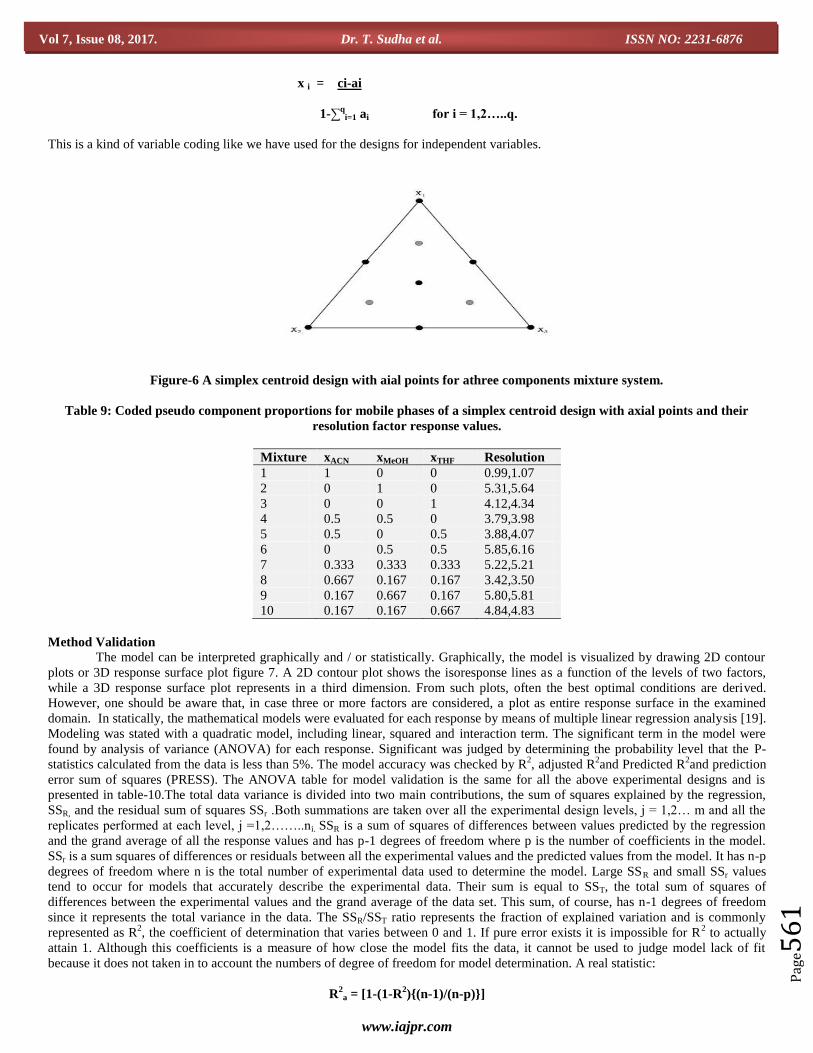
investigation of three components systems is the most common. A simplex centroid design with axial points, presented in the

concentration triangle shown in figure-6, is especially useful for ternary studies. The component proportions of the design are given in

the middle columns of table-9. Each point at a vertex of the triangle represents a pure components or a mixture of components. The

points centered on each leg of the triangle represent 1:1 binary mixtures of the components or mixtures of their neighboring vertex

points. The point in the center of the triangle represents a 1:1:1 ternary mixture of the three pure components or mixtures represented

at the vertices. The axial points contain a 2/3 portion of one of the ingredients and 1/6 portions of the other two. This simplex centroid

with axial point design is important since it permits the evaluation and validation of linear, quadratic and special cubic models. The

special cubic model for a ternary system has seven terms. The first three represents linear model, which is only valid in the absence of

interaction effects between components, i.e. ideal solutions in physical chemistry.

Ŷ = b1x1 + b2x2 + b3x3 + b12x1x2 + b13x1x3 + b23x2x3 + b12x1x2x3

The next three terms represent synergic or antagonistic binary interactions effects for all possible pairs of components and,

along with the linear terms, forms the quadratic model. The last term represents a ternary interaction effect and is usually important for

systems having maximum or minimum values in the interior of the concentration triangle. As stated earlier, each vertex can represent

a chemical mixture. In this case, the optimization involves investigating mixtures of mixtures. In liquid chromatography, these

chemical mixtures and / or pure components can be chosen to have similar chromatographic strengths or other properties that might

aid optimization. Often it is not of interest or even possible to investigate the entire range of proportion values 0 - 100%, of the

mixture components. Many mixtures optimization problems require the presence of all ingredients to form a satisfactory product. In

these cases it is convenient to define pseudo components. Consider a mixture for which the proportions of each vertex component

have to obey non – zero lower limits, which we shall generically call ai. Obviously the sum of all these limits must be less than one,

otherwise the mixture would be impossible to prepare. Considering the general case of a mixture containing q components,

q

0 ≤ ai ≤ 1 and ∑ ai < 1.

i = 1

The levels of the mixture components in terms of pseudo-components, denoted by xi, are given by the expression

www.iajpr.com

Pag

e56

1


x i = ci-ai

1-∑q

i=1 ai for i = 1,2…..q.

This is a kind of variable coding like we have used for the designs for independent variables.

Figure-6 A simplex centroid design with aial points for athree components mixture system.

Table 9: Coded pseudo component proportions for mobile phases of a simplex centroid design with axial points and their

resolution factor response values.

Mixture xACN xMeOH xTHF Resolution

1 1 0 0 0.99,1.07

2 0 1 0 5.31,5.64

3 0 0 1 4.12,4.34

4 0.5 0.5 0 3.79,3.98

5 0.5 0 0.5 3.88,4.07

6 0 0.5 0.5 5.85,6.16

7 0.333 0.333 0.333 5.22,5.21

8 0.667 0.167 0.167 3.42,3.50

9 0.167 0.667 0.167 5.80,5.81

10 0.167 0.167 0.667 4.84,4.83

Method Validation

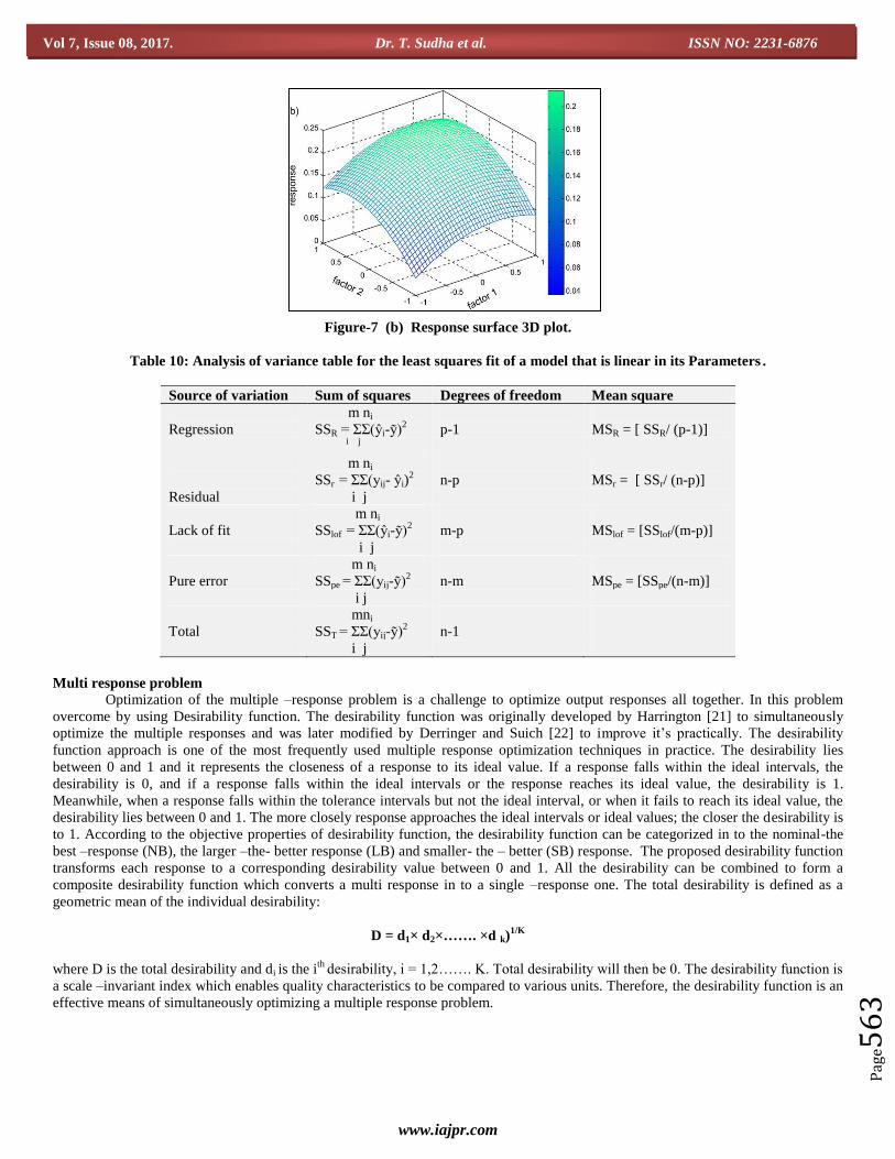
The model can be interpreted graphically and / or statistically. Graphically, the model is visualized by drawing 2D contour

plots or 3D response surface plot figure 7. A 2D contour plot shows the isoresponse lines as a function of the levels of two factors,

while a 3D response surface plot represents in a third dimension. From such plots, often the best optimal conditions are derived.

However, one should be aware that, in case three or more factors are considered, a plot as entire response surface in the examined

domain. In statically, the mathematical models were evaluated for each response by means of multiple linear regression analysis [19].

Modeling was stated with a quadratic model, including linear, squared and interaction term. The significant term in the model were

found by analysis of variance (ANOVA) for each response. Significant was judged by determining the probability level that the P-

statistics calculated from the data is less than 5%. The model accuracy was checked by R2, adjusted R

2and Predicted R

2and prediction

error sum of squares (PRESS). The ANOVA table for model validation is the same for all the above experimental designs and is

presented in table-10.The total data variance is divided into two main contributions, the sum of squares explained by the regression,

SSR, and the residual sum of squares SSr .Both summations are taken over all the experimental design levels, j = 1,2… m and all the

replicates performed at each level, j =1,2……..ni. SSR is a sum of squares of differences between values predicted by the regression

and the grand average of all the response values and has p-1 degrees of freedom where p is the number of coefficients in the model.

SSr is a sum squares of differences or residuals between all the experimental values and the predicted values from the model. It has n-p

degrees of freedom where n is the total number of experimental data used to determine the model. Large SSR and small SSr values

tend to occur for models that accurately describe the experimental data. Their sum is equal to SST, the total sum of squares of

differences between the experimental values and the grand average of the data set. This sum, of course, has n-1 degrees of freedom

since it represents the total variance in the data. The SSR/SST ratio represents the fraction of explained variation and is commonly

represented as R2, the coefficient of determination that varies between 0 and 1. If pure error exists it is impossible for R

2 to actually

attain 1. Although this coefficients is a measure of how close the model fits the data, it cannot be used to judge model lack of fit

because it does not taken in to account the numbers of degree of freedom for model determination. A real statistic:

R2a = [1-(1-R

2){(n-1)/(n-p)}]

www.iajpr.com

Pag

e56

2


makes an adjustment for the varying numbers of degree of freedom in the models being compared. Damper and Smith [20] however,

caution against its use in comparing models obtained from different data set. Model quality can only be rigorously judged if the SSr is

decomposed into two contributions, the lack of fit and the pure error sums of squares, SSlof and SSpe. The latter is a sum of differences

between all the individual experimental values and the average of the experimental values of the same level. It has n-m degrees of

freedom where m is the number of distinct levels in the experimental design. The SSlof is a sum of squares of differences between the

values predicted at each level and the average experimental value at that level and has m-p desgrees of freedom. Regression lack of fit

is determined performing an f-test by comparing SSlof/SSpe ratio with the tabled F value for m-p and n-m degrees of freedom at the

desired confidence level usually 95%. If the calculated quotient is greater than the tabled value there is evidence of model lack of fit

and the model must be discarded. If not, the model can be accepted representation of the data. Regression significance can be tested by

comparing the calculated SSR / SSr value with the tabled f- distribution value for p-1 and n-p degrees of freedom. The regression is

significant if the calculated value is greater than the tabled one. Note that this last f-test is only valid for models for which there is no

evidence of lack of fit. Finally, since the regression model does not explain experimental error the maximum percentage of

explainable variation is given by [(SST - SSpe)/ SST] X 100 %. Besides ANOVA model validation should also include an analysis of

coefficient/standard error ratios and residual plots. Terminology of the following terms and formulas used to calculate the accuracy of

the model

Std Dev:

(Root MSE) square root of the residual mean square considers to be an estimate the standard deviation.

Mean:

overall average of the all response data

Co-efficient of variation:

The standard deviation expressed as the percentage of mean. Calculated by dividing the standard deviation by the mean and

multiplying by 100.

PRESS:

Predicted residual error sum of squares –Basically a measure of how well model from this experiment is likely to predict the

response in a new experiment. Small values are desirable. The PRESS is computed first predicting where each point should from a

model that contains all other points expect the one in question. The squared residuals (difference between actual and predicted values)

are then summed.

Adjusted R2:

A measure of the amount of variation around the mean explained by the model adjusted for the number of terms in the model.

The adjusted R2 decreases the number of terms in the model increases if those additional terms don’t add value to the model.

Predicted R2:

A measure of the amount of variation in new data explained by model.

1 – (PRESS/ SStotal-SSblock)

Adequate precision:

Basically is a measure of S/N ratio (Signal to noise), it gives you a factor by which you can judge your model to see if it

adequate to navigate through the design space and be able to predict the response. Desire values > 4.0.

(Maximum predicted response- Minimum predicted response)/(Average standard deviation of all predicted responses)

Figure -7 (a). 2D Contour plot.

www.iajpr.com

Pag

e56

3


Figure-7 (b) Response surface 3D plot.

Table 10: Analysis of variance table for the least squares fit of a model that is linear in its Parameters .

Source of variation Sum of squares Degrees of freedom Mean square

Regression

m ni

SSR = ΣΣ(ŷi-ỹ)2

i j

p-1

MSR = [ SSR/ (p-1)]

Residual

m ni

SSr = ΣΣ(yij- ŷi)2

i j

n-p

MSr = [ SSr/ (n-p)]

Lack of fit

m ni

SSlof = ΣΣ(ŷi-ỹ)2

i j

m-p

MSlof = [SSlof/(m-p)]

Pure error

m ni

SSpe = ΣΣ(yij-ỹ)2

i j

n-m

MSpe = [SSpe/(n-m)]

Total

mni

SST = ΣΣ(yij-ỹ)2

i j

n-1

Multi response problem

Optimization of the multiple –response problem is a challenge to optimize output responses all together. In this problem

overcome by using Desirability function. The desirability function was originally developed by Harrington [21] to simultaneously

optimize the multiple responses and was later modified by Derringer and Suich [22] to improve it’s practically. The desirability

function approach is one of the most frequently used multiple response optimization techniques in practice. The desirability lies

between 0 and 1 and it represents the closeness of a response to its ideal value. If a response falls within the ideal intervals, the

desirability is 0, and if a response falls within the ideal intervals or the response reaches its ideal value, the desirability is 1.

Meanwhile, when a response falls within the tolerance intervals but not the ideal interval, or when it fails to reach its ideal value, the

desirability lies between 0 and 1. The more closely response approaches the ideal intervals or ideal values; the closer the desirability is

to 1. According to the objective properties of desirability function, the desirability function can be categorized in to the nominal-the

best –response (NB), the larger –the- better response (LB) and smaller- the – better (SB) response. The proposed desirability function

transforms each response to a corresponding desirability value between 0 and 1. All the desirability can be combined to form a

composite desirability function which converts a multi response in to a single –response one. The total desirability is defined as a

geometric mean of the individual desirability:

D = d1× d2×……. ×d k)1/K

where D is the total desirability and di is the ith

desirability, i = 1,2……. K. Total desirability will then be 0. The desirability function is

a scale –invariant index which enables quality characteristics to be compared to various units. Therefore, the desirability function is an

effective means of simultaneously optimizing a multiple response problem.

www.iajpr.com

Pag

e56

4


Multi criteria decision making

Developing criteria for developing the quality of chromatogram such criteria are needed in optimization procedure for high

performance liquid chromatography separations. Recently some of these criteria were critically evaluated, including the

chromatographic response factor (CRF), the chromatographic optimization function (COF), the performing power (PP), the separation

number (SN), and the product resolution (PRES).The advantages of this procedure is clear from the MCDM plot, the payoff between

the two criteria (Analysis time and resolution) is visualized, and a more rigorous decisions regarding the mobile phase composition

can be made. Because information with respect to both criteria and their pay off is available, the analyst can decide whether or not he

is willing to pay for an increase in resolution of 0.2 between the two points, an increase in the maximum capacity factor 0.94.No

preselection of a minimum resolution or analysis time is necessary. The ultimate decision as regards which mobile phase composition

to be used and can be made chromatographer after the optimization is completed. In our opinion such as decision can be made

rigorously when using the MCDM approach further research on this topic is in progress, including the extension of more than two

criteria.

CONCLUSION

Multivariate statistical techniques applied to chromatographic methods have been basically employed for optimization of the

steps of sample preparation and compound separation. The response surface techniques, the Plackett Burman designs are the best for

robustness studies where a small deviation from method condition is required and main effects only considered. Plackett- Burman can

also use for screening designs, but has the draw back that it cannot be embedded I to an optimizing design in the way of two level

factorial design can. Central composite design will continue to be popular, but if extreme at the factor space are not critical, then Box-

Behnken or Doehlert design should be considered. Statistical mixture designs are recommended for the optimization of mobile phase,

when the proportions of the components determine chromatographic peak separation and not their total amounts. Model validation

using f-distribution test, model coefficients standard errors, residual plots are used the adjusted R2 a statistic is recommended if one

must guarantee that the actual optimum experimental conditions have been found. The two level full factorial designs have often been

used for the preliminary evaluation of those experimental factors that are important for chromatographic system.

www.iajpr.com

Pag

e56

5


REFERENCES

1. Massart LD, Vandeginste MGB, Buydens CML, De jong S, Lewi JP, SmeyersJ-Verbeke. Hand book of Chemometrics and

Qualimetrics.1st ed, Elseviers, Amsterdam: 1997.

2. Vander Heyden Y, Perrin C, Massart LD. Optimization Strategies for HPLC and CZE, in: K.Valko (Ed,). Hand book of

Analytical separations, vol.1, Separation methods in Drug synthesis and purification. Elsevier, Amsterdam; 2000:163-212.

3. Joint Committee for Guides in Metrology. JCGM 200, BIPM, Serves, 2008, http://www.bipm.org/vim.

4. Skartland KL, Mjos AS, Grung B. Experimental designs for modeling retention patterns and separation efficiency in analysis of

fatty acid methyl esters by gas chromatography-mass spectrometry. Chromatogr. A.2011; 1218: 6823 -6831.

5. Zakaria P, Macka M, Fritz SJ, Haddad RP. Modelling and optimization of the electrokinetic chromatographic separation of

mixtures of organic anions and cations using poly (diallydimethyl-ammonium chloride) and hexanesulfonate as mixed

pseudostationary phase. Electrophoresis. 2002; 23 (17): 2821-2832.

6. Hibbert BD, in: Worsfold JP, Townshend A, Poole FP (Eds). Encyclopedia of Analytical sciences. Elsevier, Oxford, 2005; 469.

7. Dejagher B, Vander Heyden Y. The use of experimental design in separation sciences, Acta Chromatogr. 21.2009; 161-201.

8. Dejaeher B, Durand A, Vander Heyden Y Experimental design in method optimization and robustness testing, in :Hanrahan G,

Gomez AF (Eds) Chemometric methods in Capillary electrophoresis, John Wiley & sons, New Jersey 2010; 11-74 (chapter2).

9. Montgomery CD. Design and Analysis of Experiments, 4th

ed; New York: John Wiley; 1997

10. Lewis GA, Mathieu R, Phan-Tan-Luu .Pharmaceutical experimental design. New York: Marcel Dekker; 1999.

11. Box GEP, Hunter JS, Hunter WG. Statistics for Experiments, Second Ed; New York: Wiley –Interscience; 2005.

12. Montgomery CD. Design and Analysis of Experiments, 4th

ed; New York: John Wiley; 1997

13. Bruns RE, Scarminio IS, Neto BB. Statistical design Chemometrics, Elsevier, Amsterdam, 2006.

14. Box GEP, Wilson BK. On the experimental attainment of optimum conditions. Statistics RJ Soc.1951; 13: 1-45

15. Box GEP, Hunter SJ. Multifactor Experimental Designs for Exploring Response Surfaces. Ann. Math.Stat. 1957; 28:195.

16. Box GEP, Behnken WD. Some new three level designs for the study of quantitative variable. Technometrics 1960; 2: 455-475.

17. Doehlert HD, Klee LV. Experimental designs through level reduction of the rf-Dimensional Cuboctahedron, Discrete Math.

1972; 2: 309-334.

18. Cornell AJ, Experiments with mixtures: designs, Models and the analysis of mixture data. Wiley, New York, 1990.

19. Raissi S, Eslami Farsani R. Statistical process optimization through Multi-Response Surface Methodology. World Academy of

Sciences. Engineering and Technology. 2009; 51: 267-271.

20. Draper NR, Smith H. Applied Regression Analysis. New York: Wiley; 1981.

21. Harrington E. The desirability function, Industrial quality control. 1965; 21(10): 494-498.

22. Derringer G, Suich R. Simultaneous optimization of several response variables. J quality technology.1980; 21(4) :214-218.

54878478451170802

http://www.bipm.org/vim

Documents

REVIEW OF EXPERIMENTAL DESIGN IN ANALYTICAL CHEMISTRY