Embed Size (px)
Citation preview

REVIEW OF INTERNATIONAL ECONOMICS Manuscript No. 0745 Acceptance Date: ...... Trade performances, product quality perceptions and the estimation of trade price-elasticities +
Matthieu Crozet and Hélène Erkel-Rousse* RRH: PRODUCT QUALITY AND TRADE PRICE-ELASTICITIES LRH: Matthieu Crozet and Hélène Erkel-Rousse Abstract: Traditional trade models ignoring the dimension of product quality generally lead to excessively low trade price elasticities. In this paper, we estimate import market-share equations including a quality image proxy derived from survey data. Our estimation results, based on panel data for the four main EU member States, confirm the part played by product quality perceptions in the estimation of trade price elasticities, at least for highly differentiated products. Introducing the quality image proxy into the models leads to a significant increase in the price elasticities, which thus become superior to unity, i.e. in conformity with theoretical elasticities of substitution.
* Crozet: TEAM – CNRS, Paris I Panthéon-Sorbonne University, 106-112 Boulevard de l’Hôpital, 75657 Paris Cedex 13, France; Tel/Fax: (33) 1 44 07 82 67. E-mail: [email protected]. Erkel-Rousse: TEAM, CNRS, Paris I Panthéon-Sorbonne University, Paris, France and Direction de la Prévision (Forecasting Directorate), French Ministry of the Economy, Finance and Industry at the moment when the study was performed. E-mail : [email protected]. We thank, without implication, the French Ministry of the Economy, Finance and Industry (Direction de la Prévision - Forecasting Directorate), which financed this study, as well as the COE-CCIP, and more especially Françoise Précicaud, for having kindly provided us with data from the « Image of European Products » survey. We are also grateful to an anonymous referee for his or her fruitful remarks and suggestions on the paper.
JEL Classification: C23, F12, F14, L15.
Abbreviations: EU, R&D, COE, GDP, CIF, INTRASTAT, CHELEM, CEPII, COMEXT, UK, OLS, 2SLS, QGLS.
Numbers of figures: 0 Number of tables: 5
Date: April 5, 2003.
Address of Contact Author: Matthieu Crozet, TEAM – CNRS, Paris I Panthéon-Sorbonne University, 106-112 Boulevard de l’Hôpital, 75657 Paris Cedex 13, France; Tel/Fax: (33) 1 44 07 82 67. E-mail: [email protected].

1
1 Introduction
Most operational trade models do not take into account the “new” theory of trade and stick to the
traditional Armington (1969) framework. Such trade equations, however, often suffer from
serious estimation difficulties such as excessively low or unstable trade price elasticities, notably
suggesting specification problems (Orcutt, 1950; Harberger, 1953; Goldstein and Khan, 1985;
Madsen, 1999; Deyak, Sawyer, and Sprinkle, 1997). More generally, apart from few recent
valuable contributions (Hummels, 2000; Eaton and Kortum, 2002; Head and Ries, 2001; Baier and
Bergstrand, 2001; Clausing, 2001; Erkel-Rousse and Mirza, 2002), many estimations of trade
price elasticities lead to relatively low values in the literature.
This problem is crucial from both a theoretical and empirical point of view. Firstly, the
“new” trade theory shows that elasticities of substitution and import price elasticities are superior
to unity and tend to be equal in industries producing large numbers of varieties (Helpman and
Krugman, 1985). Secondly, several authors such as Cox and Harris (1985), Brown (1987) or
Shiells and Reinert (1993) point out that the values of trade price elasticities have a crucial
incidence on the quantitative and qualitative results of analyses performed on the basis of
multinational models. In particular, these values condition both welfare effects of trade and the
consequences of exchange rate policies, as well as the macroeconomic regulation of open
economies in general.
Traditionally, this problem has been addressed by stressing the crucial part of both
imperfect measurement of trade prices and potential endogeneity problems on trade price
elasticity estimation1. In this paper, we suggest that these unquestionable causes for low price
elasticities might not be exclusive. More precisely, we show that ignoring vertical product
differentiation in trade equations also leads to under-estimated price elasticities. The underlying
intuition is easy to understand. In fact, adding a quality variable into a market share equation
would enable one to suppress the (positive) indirect effect of product quality through prices from

2
the (negative) overall relative price effect. The relative price contribution would thus become a
pure price effect, which has an unambiguous negative impact on market shares, while the overall
positive influence of product quality would be captured by the quality factor.
In practice, the quantitative impact of ignoring product quality might be relatively high in
vertically differentiated industries (Shaked and Sutton, 1984; Falvey and Kierzkowski, 1987), in
such a way that it be significant at macroeconomic level. In this respect, an empirical study
performed by Fontagné, Freudenberg and Péridy (1998) confirms the increasing share of trade in
vertically differentiated products in total trade, especially within the European Union (EU).
Unfortunately, product quality is usually unobservable, so that introducing such a variable
into trade equations requires the definition of a proxy. Many authors use proxies based on R&D
expenses or human capital variables (Greenhalgh, Taylor, and Wilson, 1994; Eaton and Kortum,
2002; Ioannidis and Schreyer, 1997; also see other references below). Such indirect measures of
product quality may a priori differ from what they are supposed to capture or, at least, focus on a
specific dimension of product quality, namely technological differentiation. As far as the present
study is concerned, we have had the opportunity to use a direct measure of quality perceptions or
« images » relating to products originating from the four main EU countries and derived from a
survey performed by the Centre d’Observation Economique (COE) of the Chambre de Commerce
et d’Industrie de Paris on a European basis. Our estimations lead to results in conformity with
intuition. Controlling a market share equation for product quality perceptions enables us to obtain
a significant increase in trade price elasticity; the price elasticity thus becomes superior to unity.
We obtain this result without changing our relative price index. In this respect our approach
differs from that of Feenstra (1994), who modifies his trade price index to take product variety
into account. We then replace our quality proxy with an innovation perception proxy derived from
the same survey, for comparison purpose. Results of models using the former or the latter proxies
prove to be very much alike. This comparison provides one with a significant even though fragile

3
ex post argument in favour of using indirect quality image proxies based on innovation variables
as a second best solution.
2. The theoretical model
In this section we present a trade model derived from Erkel-Rousse (1997, 2002), which leads to
the determination of a testable market-share equation.
Assume there are 2≥I trading countries, producing and exchanging K differentiated
products k = 1,...,K. The representative consumer of country j, ,,...,1 Ij∈ maximises a Spence-
Dixit-Stiglitz sub-utility function kjU subject to his or her budget constraint:
)1(
1 1
)1(
−
= ∑∑
= =
−
σσ
σσαI
i
n
vvijkijkj
ki
yU (1)
where vijy stands for total demand of variety v addressed to its producer in country i and kin for
the number of varieties originated from country i. σ is the elasticity of substitution between
domestic and imported goods from different origins. Preference parameters ( )Iikij ,...,1=
α can be
viewed as the quality perceptions or images of product varieties originating from country i. They
depend on the intrinsic quality of varieties produced in country i, but also on the representative
consumer in country j’s purely subjective perceptions (as regards product desirability), which may
differ from one importing country to another. Note that our reading of preference weights
therefore encompasses the alternative interpretations given by Feenstra (1994) (in terms of
product quality) and Head and Mayer (2000) (in reference to home bias or typical aversion to
foreign products).
Preference parameters are equal for all varieties of product k originating from the same
country i. This property stems from the fact that preference parameters are supposed to essentially
derive from national differences in terms of production technologies and know-how. Conversely,
we assume that firms from a given country face the same production conditions.

4
Total production of variety ( , )v i is broken down between markets ( , )k j , j = 1,...,I:
∑=
+=I
jvijkijvi yty
1
)1(
where vijy stands for the production share of variety ( , )v i sold on market ( , )k j , which is
identical to the demand expressed on this market at equilibrium. The combination of transport
and transaction costs is viewed as the destruction of a part ( vijkij yt ) of the production shipped
towards market ( , )k j during the transportation from country i to country j (“iceberg”
representation).
Production and transport conditions being identical for every variety ( , )v i , the latter are
sold in equal quantities kijvij yy ≡ and at the same price kijvij pp ≡ on market ( , )k j . From the
producer profit maximisation, one derives the well known price expression:
)1()1( −+= kijkijijkikij tcp εε (2)
where kic denotes the unit cost of producing a variety of product k in country i and
( ) ( )kijkijkijkijkij ppyy // ∂∂ε −≡ the price elasticity of demand for variety ( , )v i in country j. The
expression of kijε is calculated on the basis of demand functions. The latter are derived from the
first-order conditions associated with maximisation of (1) under the consumer budget constraint:
( ) ( )kjkjjki
I
ikikijkjkijkij pEnppy
= ∑=
− σσσ αα '1'
' (3)
where, as is shown in Hickman and Lau (1973), )1(1
11
1σ
σσσ αα−
==
−
= ∑∑I
ikijki
I
ikijkijkikj npnp stands for
the average price of product k on market ( , )k j and kjE for the share of country j’s national
revenue allocated to the consumption of product k. The higher the elasticity of substitution σ , the
more sensitive demands to relative prices and quality images. Partial derivations of (3) lead to:
5
−−+= −
=
− ∑ σσσσ αασε 1''
1''
11)1(1 jkijki
I
ikikijkijkij pnp (4)
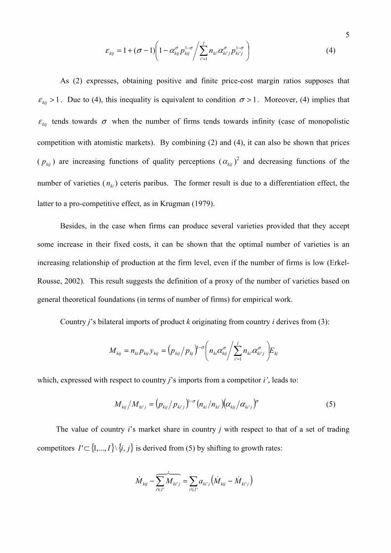
As (2) expresses, obtaining positive and finite price-cost margin ratios supposes that
1>kijε . Due to (4), this inequality is equivalent to condition 1>σ . Moreover, (4) implies that
kijε tends towards σ when the number of firms tends towards infinity (case of monopolistic
competition with atomistic markets). By combining (2) and (4), it can also be shown that prices
( kijp ) are increasing functions of quality perceptions ( kijα )2 and decreasing functions of the
number of varieties ( kin ) ceteris paribus. The former result is due to a differentiation effect, the
latter to a pro-competitive effect, as in Krugman (1979).
Besides, in the case when firms can produce several varieties provided that they accept
some increase in their fixed costs, it can be shown that the optimal number of varieties is an
increasing relationship of production at the firm level, even if the number of firms is low (Erkel-
Rousse, 2002). This result suggests the definition of a proxy of the number of varieties based on
general theoretical foundations (in terms of number of firms) for empirical work.
Country j’s bilateral imports of product k originating from country i derives from (3):
( ) kjjki
I
ikikijkikjkijkijkijkikij EnnppypnM
== ∑=
− σσσ αα '1'
'1
which, expressed with respect to country j’s imports from a competitor i’, leads to:
( ) ( )( )σσ αα jkikijkikijkikijjkikij nnppMM ''1
''−= (5)
The value of country i’s market share in country j with respect to that of a set of trading
competitors jiII ,\,...,1'⊂ is derived from (5) by shifting to growth rates:
( )∑∑∈∈
−=−''
''''
'Ii
jkikijjkiIi
jkikij MMaMM &&48476
&.

6
with ∑∈
='
''Il
kljjkijki MMa , aki ji I
'' '
=∈∑ 1,
where time index t is implicit (as is the case in the whole section). Note that, if reasoning in
discrete time, we would have to replace the )( ' jkia coefficients with their lagged values.
Transforming (5) into growth rates and then integrating (which introduces an invariant factor
'kijIc ), we obtain:
( ) ( ) ( ) ( ) ''''' )1( kijIkijIkijIkijIkijI cimageqLogietyvarLogpriceLogmshareLog +++−−= σσ (6)
where: ,''
'' ∑∈
=Ii
jkikijkijI MMmshare ,'' jkIkijkijI ppprice = ,'' kIkikijI nnietyvar = and
jkIkijkijIimageq '' αα= ( p p n nkI j ki ji I
akI ki
i I
aki j ki j
' ''
' ''
' ', ,= =∈ ∈∏ ∏ and α αkI j ki j
i I
aki j' '
'
'=∈∏ standing for,
respectively, the average import price, number and quality image of varieties originating from the
set of i’s competitors I’).
Consequently, in this model, relative market shares depend on relative prices as well as
two differentiation terms, the relative quality image and number of varieties, plus an invariant
factor. Therefore, exporters can increase their market shares by lowering their prices with respect
to those of their foreign competitors, or by reinforcing their relative differentiation effort in order
to raise their relative number of varieties or modify their relative image of quality to their
advantage. Note that the coefficient of the price factor in (6) is strictly negative, due to condition
1>σ .
3 Toward a testable trade equation.
Equation (6) has to be transformed into a testable equation. In this respect, two crucial points
have to be mentioned.
Firstly, trade prices are measured with error through unit values of trade, which may cause
correlations between this imperfectly measured explanatory variable and the perturbation of the

7
model. Note however that we have calculated unit values of trade not only in time variations but
also in cross-section. In other terms, we expect to capture at least part of the spatial dimension of
prices. This is a consequential point due to the potentially important influence of spatial effects in
panel modelling. Besides, we have considered that import unit values would be a more
convincing approximation for bilateral prices than export unit values, as the former take into
account price competition between exporters at the entry of market j (transport and other
transaction costs from any exporting country to market j being included in CIF import unit
values)3. For the same reason, import declarations have been chosen as a theoretically more
satisfactory measurement of bilateral trade flows than export declarations in the context of our
model. Note that the under-estimation of intra-European import declarations since the creation of
the INTRASTAT system of measurement of intra-EU trade flows in 1993 should be notably
limited by the definition of the dependent variable of our trade equation, which is based on a ratio
of imports (rather than on import levels). All trade variables have been calculated on the basis of
six-digit data originating from the COMEXT data base of Eurostat. On this basis, we have
calculated more aggregated trade flows corresponding to the nomenclature of the COE survey.
Secondly, differentiation terms ( kitn ) and ( kijtα ) - where time index t is now explicit - are
unobservable. Omitting these factors or pretending to capture them through fixed effects might
lead to a biased price elasticity and consequently to a bad evaluation of the elasticity of
substitution σ , especially in highly differentiated industries. Therefore, we have decided to build
proxies of these explanatory factors. As will be explained below, our focusing on the four biggest
EU countries (France, Germany, Italy, United Kingdom) results from the availability of quality
image measures in the case of these member States. Consequently, for each couple of countries
(i,j) considered among this set of four member States, the sub-set of competitors I’ of the
theoretical model will be restricted to the two other EU countries.

8
The quality image proxy derives from the “Image of European products” annual survey of
the COE. This survey consists in interviewing a panel of importers from different EU member
States concerning their perceptions of the relative characteristic features of products originating
from other EU countries in their sectors of activity. Specific questions notably deal with product
quality, notoriety, degree of innovation, price, and ratio of quality to price, depending on
geographic origin. This exceptional source therefore provides us with a purely exogenous piece of
information on perceived quality with respect to trade data. Moreover, quality images collected
from this survey depend on both the intrinsic quality of products and importers’ subjective
perceptions, which may differ significantly from one importing country to the other. In this
respect, bilateral quality images which result from the COE survey are perfectly consistent with
the theoretical preference parameters ( kijtα ).
Survey data refer to years 1992 to 1997 for different kinds of products, namely “consumer
goods” (split up into four sub-sectors: food, hygiene, lodging and clothing), and “other goods”
(consisting of three sub-sectors: raw intermediate products, mechanical goods and electric goods
other than consumer products) – Cf. Appendix 1. As was mentioned above, we have focused on
the four main EU countries (as producing and purchasing countries), for which the COE survey
results are available on a sufficiently long period and can be considered to be enough robust. Our
quality image proxy is calculated on the basis of the answers to the four questions: “In terms of
quality levels, do you think that French / German / British / Italian products are: - the most
competitive ones (mark = 1) - as competitive as those from other countries (mark = 2) - less
competitive than those from other countries (mark = 3) - not competitive at all (mark = 4)?”.
Each interviewed importer is supposed to answer this question for products from every
geographic origin, except from his or her own country. Let kijtimqual denote the percentage of
interviewed importers from country j in sector k answering 1 or 2 to the question relating to

9
country i in the survey performed in year t −1 . We define the proxy for relative quality image
( jtkIkijttkijIimageq '' /αα= ) as:
jtkIkijttkijI imqualimqualgeqaim ''~ ≡
using the formula defining every theoretical explanatory variable in (6), including tkijIimageq ' , with
jkia
IijtkijtkI imqualimqual '
''' ∏
∈
≡ and jiKingdomUnitedItalyGermanyFranceI ,\,,,'= . Weights
)( ' jkia , defined in section 2, are relating to 1991 in order to avoid endogeneity problems.
Although )~( 'tkijIgeqaimLog does not derive from a quantitative measurement of quality images, we
expect it to be at least positively correlated with ).( 'tkijIimageqLog However, several technical
points deserve some comments.
The reason for defining kijtimqual on the basis of the survey relating to year t −1
originates from the fact that COE surveys are performed in October, i.e. late each year.
Therefore, we consider that a survey performed in October of year t might reveal quality images
which are closer to those operating in year t +1 than in year t in terms of consumer choices.
Above all, this choice may protect us from possible endogeneity problems during the estimation
process.
It might seem more intuitive to define kijtimqual on the basis of responses to mark 1 only,
or at least to over-weight percentages of marks 1 with respect to those of marks 2 in the calculus
of kijtimqual . We experimented all these alternatives, using several possible weights. However,
the indicator that we finally chose proved to lead to more convincing results, due without doubt to
its higher robustness. In fact, cumulated percentages of marks 1 and 2 prove to be much more
regular over time than percentages of marks 1 (respectively 2) alone, which are more volatile. We
find the same result concerning cumulated percentages of marks 3 and 4 compared to those of
marks 3 and 4 considered separately. This property of the COE survey results suggests that the
10
interviewed have a clearly positive or negative opinion concerning products from other EU
countries, but not as qualified as to choose without doubt between the two positive (or two
negative) modalities of questions asked in the COE survey. Our definition of the quality image
proxy takes this characteristic feature of the survey data into account.
Ignored by the theoretical model, multinational companies, intra-firm trade and vertical
integration may loosen the link between national product quality perceptions and geographic
origins of trade flows. The fact that the surveyed are import professionals (who can be viewed as
“experts” in their field) does limit the difficulty, but may not suppress it. This constitutes a
possible limitation to the present study.
COE surveys successively deal with consumer goods (1992, 1994, 1996) and “other”
goods (1993, 1995, 1997). Therefore, we have had to reconstitute annual indicators from biennial
( kijtimqual ). Assuming that national quality images are relatively stable structural variables
(which is confirmed by the evolution of our proxy), we have filled missing years with the simple
arithmetic means of two successive biennial indicators.
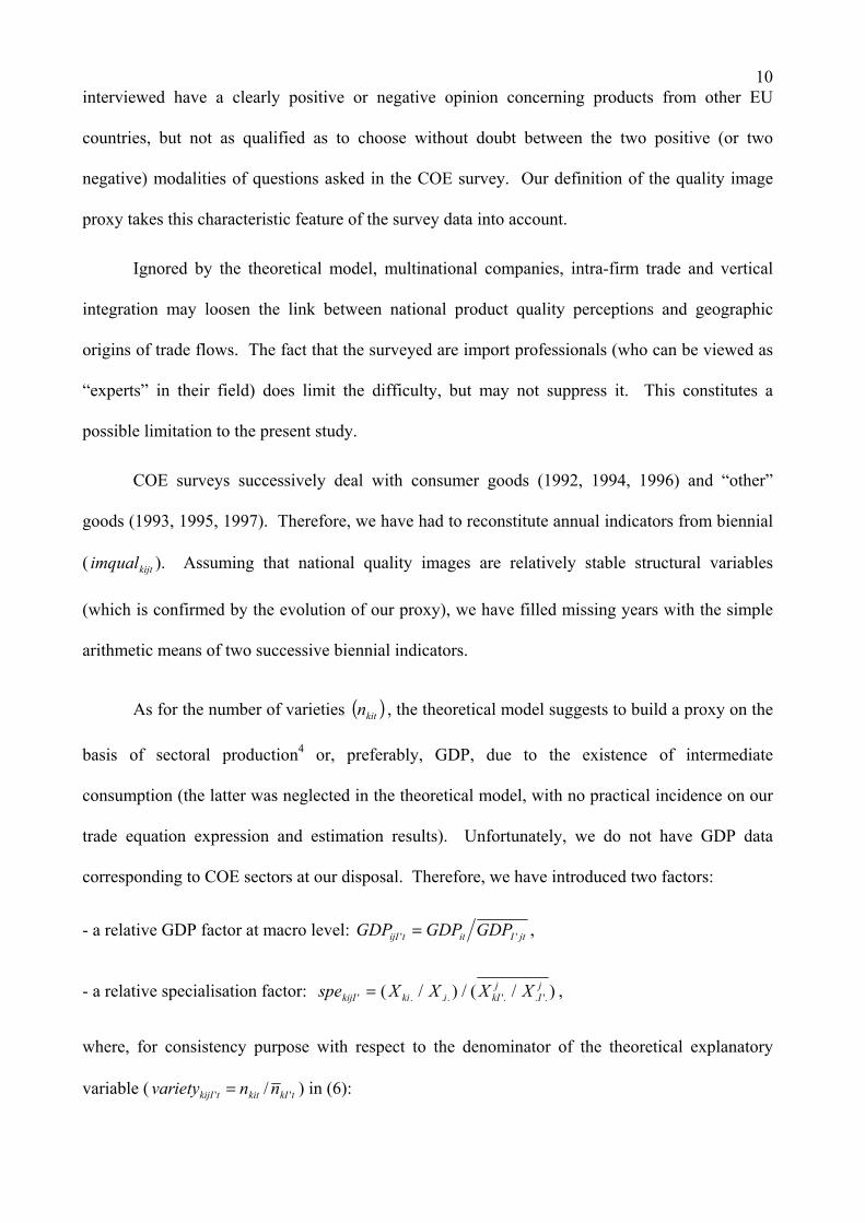
As for the number of varieties ( )kitn , the theoretical model suggests to build a proxy on the
basis of sectoral production4 or, preferably, GDP, due to the existence of intermediate
consumption (the latter was neglected in the theoretical model, with no practical incidence on our
trade equation expression and estimation results). Unfortunately, we do not have GDP data
corresponding to COE sectors at our disposal. Therefore, we have introduced two factors:
- a relative GDP factor at macro level: jtIittijI GDPGDPGDP '' = ,
- a relative specialisation factor: spe X X X XkijI ki i kIj
Ij
' . . . '. . '.( / ) / ( / )= ,
where, for consistency purpose with respect to the denominator of the theoretical explanatory
variable ( tkIkittkijI nnietyvar '' /= ) in (6):

11
jkia
IitijtI GDPGDP '
'''' ∏
∈
= and ( / )'. . '.X XkIj
Ij = ( )X Xki i
i I
aki j
'. . '.' '
/ '
∈∏ .
The relative specialisation factor proxies the unobserved sector structure of GDP through
that of exports. The closer and the more stable the structures of national GDPs in terms of
tradable and non tradable products, the more satisfactory this approximation. As the countries
taken into account are highly integrated European member States of relatively comparable sizes,
we have assumed that this approximation was acceptable. In this case, the product of the two
preceding factors constitutes a proxy for relative GDP (and consequently for the relative number
of varieties tkijIietyvar ' ) at sector level. However, due to the approximation made, as well as to the
fact that the specialisation factor has been calculated on a reference year (1991) rather than on a
current basis5, we have tested a trade equation in which the logarithms of these two factors are
introduced separately. Therefore, it is possible to check whether the estimated coefficients of
these two explanatory variables are similar (in conformity to intuition) or not.
National GDP data, expressed in 1991 prices, derive from the CHELEM data base of the
CEPII. They have been smoothed over three years ( t t, −1 and t − 2 ) in order to capture the
structural dimension of product variety rather than short-term economic fluctuations: the weights
used in the smoothing are respectively 0.3, 0.4 and 0.3 for t t, −1 and t − 2 . Overall export data
by sector ( .klX ) and at macro level ( ..lX ) in 1991 originate from export declarations of the
COMEXT data base.
Finally, we have replaced the invariant factor 'kijIc with a linear combination of
miscellaneous fixed effects, an intercept and a relative distance effect ( jIijijI distdistdist '' /= )
based on a ratio of absolute distances, the absolute distance between two countries i’ and j (noted
jidist ' , iIi ∪∈ '' ) being defined as that between the latter countries’ two capital towns. Note that,
as relative unit values of trade are not indices, distance is not supposed to capture part of relative

12
transport costs, unlike in many gravity models. Moreover, as our proxy for relative quality image
encompasses importers’ subjective perceptions, distance is in principle not needed either to
capture part of the latter. Nonetheless, as is suggested by Anderson and Marcouiller (1999) or
Rauch (1999), introducing relative distance may enable us to capture other kinds of obstacles to
trade than those taken into account through relative prices, or more probably (within a EU country
sample) to limit the estimation effects of imperfect price and quality image measurements.
To sum up, the non restricted equation to be estimated is:
( ) ( ) ( )
( ) ( ) tkijIijIdtkijIq
kijIstijIgtkijIptkijI
uerceptinteffectsfixeddistLogegeqaimLoge
speLogeGDPLogeceiprLogemshareLog
'''
''''
~
)(~)1(
+++−+
++−−= (7)
The parameters of interest (referred to by e) may not be equal to the theoretical coefficients
as all explanatory variables are proxies. However, the theoretical model gives some indications
on the expected values for the estimated coefficients that should be satisfied so as to be considered
to be convincing. The price elasticity pe should be homogeneous to an elasticity of substitution
σ, i.e. be strictly superior to unity. The coefficients associated with the variety proxies ( ge and
se ) should be of the same order of magnitude. They should also be either equal to unity (in
accordance with Krugman, 1980) or, at least, inferior or equal to unity (in accordance with a
modified version of our theoretical framework allowing for multi-variety producing firms6).
However, the fact that relative GDP varies across time while the specialisation variable does not
may induce some coefficient asymmetry. That is why we have tested the non restricted equation
(7) in which ge and se are not a priori set to be equal. The coefficient of the quality image proxy
( qe ) should be strictly positive. Its value depends notably on the elasticity of substitution between
varieties as well as the correlation between the proxy and the true relative quality image, which
may significantly differ from unity, due to the qualitative foundation of the ( kijtimqual )

13
percentages. Finally, the coefficient of relative distance ( de ) should be negative and probably
close to zero.
The perturbation ukijI t' originates from the difference between theoretical variables and
proxies. ukijI t' also takes into account possible exceptional events and the parts of potential
missing variables that are orthogonal to our explanatory factors. Time index t corresponds to
years 1993 (or 1994) to 1997. Note that we « loose » the first year when COE survey data are
available, namely 1992 (consumer goods) or 1993 (other goods), due to the construction of the
quality image proxy (the kijtimqual percentages being set to be relating to the COE survey
performed in year t −1). Country indices i j, are relating to France, Germany, Italy, or the UK,
while sector index k represents either food, clothing, hygiene, lodging, raw intermediate products,
mechanical goods, or electrical goods other than consumer goods. In sum, we have
5 × 4 × 3 × 4 = 240 observations for consumer goods and 4 × 4 × 3 × 3 = 144 for other goods.
We have performed two sets of estimations: one on consumer goods, on the 1993-1997
estimation period, and the other pooling all goods together, from 1994 to 1997 (i.e. using
240 48 144 336− + = observations). Each set of estimations has been compared with the results
derived from a more traditional sub-model excluding the quality image variable ( qe restricted to
zero), or both dimensions of product differentiation ( qe , ge and se restricted to zero). The
interesting aspect of such comparisons is that the latter enable us to study how estimated price
elasticities are modified when the adding of relative quality image (respectively differentiation
variables) into the model suppresses at least part of the quality (respectively product
differentiation) dimension contained in the relative price effect.
Finally, we have estimated equation (7) using three alternative sets of econometric
methods, to test the robustness of the results. Firstly, we have performed ordinary least squares
(OLS). Secondly, we have tested different instrumental variable estimation methods (hereafter

14
referred to as 2SLS, for 2 Stage Least Squares). In fact, the differentiation and price variables are
measured with error. Moreover, their exogenous status is highly questionable. Therefore, they
have been instrumented by the first lag of the relative price and GDP variables, as well as the
unvarying factors of the model (the intercept, specialisation, distance, and the fixed effects which
are included in the model, when there are some), plus an instrument for quality image defined in
the same way as the quality image proxy, but where the imqualklj percentages are calculated on the
basis of the results derived from the first available survey (namely 1992 for consumer goods and
1993 for other goods). In order to limit the risk of correlation between this variable and the
perturbation of the model, we have performed this instrumental variable method on 1995-1997 for
consumer goods, and 1996-1997 for the whole sample. Opting for these restricted estimation
periods have enabled us to suppress any reference to the 1992 and 1993 surveys in imageq kijI$ ' and,
consequently, in the current perturbation ukijI t' (remember that percentages imqualkijt are set to be
relating to the COE survey performed in year t-1). Thirdly, to suppress heteroskedasticity and
correlation from our estimation residuals, we have performed two quasi-generalised least square
alternative methods, referred to as QGLS 1 and QGLS 2 and presented in Appendix 2. All these
estimation methods lead to very similar results, which can be viewed as a sign of robustness.
4 Main estimation results
Our main estimation results are summarised in Tables 1 (consumer goods alone), 2 (all goods
pooled together), and 3 (models without fixed effects). Coefficients’ estimates are little affected
by the econometric methods. However, when QGLS methods are applied, variances estimations
drop sharply, which may modify the results of the significance and inequality tests. More
interesting, results of models including quality image appear to be much more satisfactory than
those of models excluding this variable.

15
Firstly, in equations taking quality image into account, the coefficient relating to the
quality image proxy appears to be clearly significant and of the expected positive sign7.
Secondly, models including quality image show a very positive property: their estimated
price elasticities are strictly superior to unity, thus taking values in conformity with the underlying
theoretical model. Note that these estimated price elasticities (around 1.2) are close to those
obtained by authors using other quality proxies (Erkel-Rousse and Le Gallo; 2002), and of the
same order of magnitude as those obtained by authors using innovation variables such as R&D
expenses or numbers of patents (Greenhalgh, Taylor and Wilson, 1994; Magnier and Toujas-
Bernate, 1994; Ioannidis and Schreyer, 1997; Anderton, 1999). Above all, they are superior to
those obtained in models excluding quality image (see below). The increase in the price elasticity
when adding quality image is easy to interpret. In models excluding quality images, the
coefficient relating to the price factor takes into account a pure price effect (which is negative)
plus the indirect positive incidence of product quality on market shares through prices ceteris
paribus (therefore, the sum of the two effects is less negative than the pure price effect). When
quality image is taken into account, its coefficient captures this indirect effect, which disappears
from the price coefficient. The latter then becomes a « pure » price elasticity, which is
homogeneous to an elasticity of substitution (and therefore must be superior to unity).
Besides, the coefficients associated with relative GDP and specialisation are systematically
inferior to unity (between 0.3 and 0.6, depending on the model), which is consistent with a version
of our theoretical framework allowing for multi-variety producing firms, as was explained above.
In most models with fixed effects, the coefficient relating to GDP (around 0.6 or 0.7) is higher
than that relating to the specialisation variable (around 0.3). As was stressed before, the
asymmetric definition of the GDP and specialisation variables (the former being allowed to vary
across time, contrarily to the latter) may break the expected similarity of their two coefficients.
However, in most models without fixed effects (table 3), the two coefficients are very much alike

16
(between 0.4 and 0.5), especially when all products are pooled together within the panel (for
instance, the two coefficients derived from QGLS 1 are equal to, respectively, 0.47 and 0.49).
When the proxy for quality image is excluded from the model, as is the case in most
empirical work on trade equations, several problems show up.
The estimated price elasticity drops significantly below unity, whatever the model and the
econometric technique. As was explained above, the price elasticity here captures part of the
positive quality effect on market shares, which explains its lower absolute value (of around 0.8 or
0.9, depending on the model). This is a crucial problem as the price coefficient can no longer be
interpreted as an elasticity of substitution. Nor can it be easily linked to any other parameter of
interest derived from the underlying theoretical model. If one had obtained such an estimated
equation on the basis of a theoretical framework excluding vertical differentiation, the (apparent)
inconsistency between the value taken by the estimated price elasticity and its expected order of
magnitude (which should in any case be superior to unity) would have (rightly) suggested a
specification problem.
In the models including fixed effects and the two variety proxies, the coefficient associated
with relative GDP is now higher than expected. First, it is significantly superior to unity (around
1.2 or 1.3, depending on sectors taken into account), which is not consistent with theory (see
above). This result should shed doubt on the validity of the estimations, as the two alternative
theoretical foundations for the variety proxy used require that the elasticity of variety to
production be either equal or inferior to unity. Moreover, the coefficient of relative GDP is often
about twice as high as that relating to specialisation (which amounts to 0.7), while it should be of
the same order of magnitude. In this respect, the coefficient associated with specialisation proves
to be in conformity with the theoretical model. The problem definitely lies in the excessive value
of the GDP coefficient. Remember, however, that the estimated value of this coefficient is
notably affected by the presence of fixed effects (contrarily to the other parameters of interest). In

17
fact, when fixed effects are excluded from the model, it becomes slightly inferior to unity (or even
to 0.9 in the consumer good model) and closer to the specialisation coefficient (the latter then
being close to 0.8) (table 3).
Last but not least, the way the price elasticity is modified when the variety proxies are
excluded from the model may seem somewhat puzzling, at least at first sight. In fact, it can be
shown that excluding variety from the market share equation leads to a modification of the
theoretical price elasticity, the latter now encompassing both the price effect corresponding to the
price elasticity in the model including variety plus the indirect incidence of variety on market
shares through prices everything else being unchanged in the model. One can establish that the
sign of this indirect effect depends on that of the partial correlation between prices and variety,
ceteris paribus in the trade equation. This partial correlation can be seen as the linear equivalent
of the (non linear) partial derivative of prices with respect to variety in the underlying theoretical
model8. According to the latter, a rise in the number of varieties ceteris paribus should imply a
drop in prices due to higher competition: in other terms, the partial derivative of prices with
respect to variety is negative. Therefore, we can reasonably9 expect the partial correlation
between prices and variety to be negative, at least if the model is correctly specified10. Such a
negative correlation implies that the price elasticity should be higher in equations excluding the
variety proxies than in equations including them. Unfortunately, this property is not satisfied in
the case of the equations excluding quality image (when the variety proxies are removed from the
equation, the price elasticity decreases by more than 0.1). This counterintuitive result again
suggests a specification error. Here again, the adding of the quality image proxy in the model
solves this problem. In fact, in equations taking quality image into account, the excluding of the
variety proxies leads to a slight, but significant, decrease in the price elasticity (of 0.05 or more,
depending on the model), which is consistent with intuition. In reality, the intuition does not hold
in equations excluding quality image because the price and variety effects encompass part of the
quality image effect, instead of limiting themselves to pure price and variety effects.

18
Note that adding quality image induces a significant drop in the variety coefficients (by
more than 40%), whatever the specification of the model. In fact, in equations excluding quality
image, the coefficients of the variety proxies encompass a direct variety effect plus the indirect
incidence of quality on market shares through variety everything else being unchanged in the
model. Adding quality image in the equation leads to the suppression of this indirect effect from
the variety coefficients. It can be shown that this indirect effect is of the sign of the partial
correlation between variety and quality image, ceteris paribus in the equation (the argument being
the same as that used above for prices and variety). The drop in the coefficients relating to the
variety proxies implies that this partial correlation is negative, which might originate from the
trade-off between variety and quality often suggested in theoretical models of product
differentiation11.
Table 4 illustrates the specific feature of raw intermediate products. In this sector of
almost homogeneous products, price elasticity (which reaches values between 2.1 and 2.6,
depending on the model) proves to be notably higher than in other sectors. Moreover, export
performances seem to be essentially driven by low relative prices, contrarily to what happens for
consumer goods, as well as for equipment and other intermediate goods.
5. Quality image versus innovation image
Responses to the following question of the COE survey: “In terms of innovation, do you think that
French / German / British / Italian products are: - the most competitive ones (mark = 1) - as
competitive as those from other countries (mark = 2) - less competitive than those from other
countries (mark = 3) - not competitive at all (mark = 4)?” enable us to build an innovation image
proxy on the same basis as the quality image proxy. This innovation image proxy proves to be
highly correlated with that of quality image. This result is interesting as many theoretical models
derived from the new trade theory establish a tight link between quality and innovation.

19
Moreover, several authors use R&D, the number of patents, or other innovation variables as
proxies of quality in trade equations (Greenhalgh, Taylor, and Wilson, 1994; Magnier and Toujas-
Bernate, 1994; Amable and Verspagen, 1995; Anderton, 1999; Carlin, Glyn and Van Reenen
1997; Eaton and Kortum, 2002; Ioannidis and Schreyer, 1997). Conversely, Fontagné,
Freudenberg and Ünal-Kesenci (1998) suggest that trade specialisation in quality does not
coincide with that in technological products. However, the approach of COE survey (like that of
the formerly mentioned literature) differs radically from that of Fontagné et alii. In fact, the
survey examines the innovation image of any set of products, while Fontagné and alii focus on
technological products.
We have performed a set of estimations using image proxies based on innovation instead
of quality, for comparison purpose. Whatever the panel (consumer goods or all products pooled
together), we find the same qualitative results when replacing quality image with the innovation
proxy. As far as consumer goods are concerned, the econometric adjustment seems to be slightly
better when using the quality variable (table 5). Besides, an attempt to include both quality and
innovation into the model suggests that the quality variable might dominate as an explanatory
variable for market shares. However, an ambiguous collinearity diagnosis between quality and
innovation sheds doubt on the robustness of this result. In addition, estimations performed on the
whole sample no longer suggest any superiority of the quality criterion over that relating to
innovation. As the degree of collinearity between quality and innovation is much higher for raw
intermediate goods and for capital goods than for consumer goods, it becomes impossible to
evaluate which of the two criteria might be preferable.
The product-cycle hypothesis might play a role in these results (Feenstra and Rose, 2000).
In any case, these estimations suggest that, had the quality variable not been available, the choice
of a proxy based on the innovation criterion would have led to very similar results, which argues
in favour of the empirical literature mentioned above. However, we must be cautious as regards

20
the general incidence of our results. In fact, our innovation criterion might well be much closer to
our quality criterion than any other innovation indicator based on R&D expenses or the number of
patents...
6 Conclusion
In this paper, we have aimed at showing that more convincing estimated trade price elasticities
can be obtained by controlling product quality in trade equations. In this purpose, we have
estimated trade equations including a quality image proxy derived from survey data. Our
estimation results, based on panel data for the four main EU Member States, confirm our initial
intuition. A contrario, these results suggest that traditional models (especially macro-econometric
ones) ignoring the dimension of product quality lead to under-estimated trade price elasticities and
thus to incorrect evaluations of economic policy implications in open countries.
One might expect true price elasticities to be even higher than those derived from our
estimations, at least for the most competitive industries. In fact, our approach has not led to as
high price elasticities as those (estimated using different methodologies and kinds of data) by
Hummels (2000), Head and Ries (2001), Eaton and Kortum (2002), Baier and Bergstrand (2001),
Clausing (2001), or Erkel-Rousse and Mirza (2002) for instance. Moreover, low mark-up
estimates or account rates of return are usually observed at industry levels (see Schmalensee,
1989, and Bresnahan, 1989), which may be consistent with relatively high levels of substitution
elasticities, at least in industries characterized by monopolistic competition. We could probably
obtain higher price elasticities, had we both more accurate proxies of quality perceptions and
better measures of relative prices at our disposal, or at least could we build more sophisticated
instruments for the latter. However, even in such an ideal context, we might need more broken-up
data as well. Now, we have had to stick to the relatively aggregated product classification of the
COE survey in this respect, which, besides, has prevented us from studying industry and country
heterogeneity thoroughly.

21
Results obtained when using the economic approach consisting in taking product quality
into account or, alternatively, an econometric method based on the definition of sophisticated
instrumental variables for trade prices suggest that each approach succeeds in correcting part of
the under-estimation of price elasticities, but not the whole of it. Unfortunately, up to now (at
least to our knowledge), there has not been available direct broken-up quality measures which
would enable one to mix the two methodologies.

22
References Amable, Bruno and Bart Verspagen, “The Role of Technology in Market Shares Dynamics,” Applied
Economics 27 (1995):197-204.
Anderson, James E. and Douglas W. Marcouiller, “Trade, Insecurity, and Home Bias: An Empirical
Investigation,” National Bureau of Economic Research Working Paper No. 7000, 1999.
Anderton, Bob, “Innovation, Product Quality, Variety, and Trade Performance: an Empirical Analysis of
Germany and the UK,” Oxford economic papers 51 (1999):152-67.
Armington, Paul S., “A Theory of Demand for Products Distinguished by Place of Production,” IMF Staff
Papers 16 (1969):159-78.
Baier, Scott L. and Jeffrey H. Bergstrand, “The Growth of World Trade: Tariffs, Transport Costs, and
Income Similarity,” Journal of International Economics 53 (2001):1-27.
Bresnahan, Timothy F., “Empirical Studies of Industries with Market Power,” in Richard Schmalensee
and Robert Willig (eds.), Handbook of Industrial Economics volume 2, Amsterdam: North Holland,
(1989): 1011-57.
Brown, Drusilla. K., “Tariffs, the Terms of Trade, and National Product Differentiation,” Journal of Policy
Modeling 9 (1987): 503-26.
Carlin, Wendy, Andrew J. Glyn and John Van Reenen, “Quantifying a Dangerous Obsession?
Competitiveness and Export Performance in an OECD Panel of Industries,” CEPR Discussion Paper No.
1628, 1997.
Clausing, Kimberly A., “Trade Creation and Trade Diversion in the Canada-United States Free Trade
Agreement,” Canadian Journal of Economics 34 (2001): 677-96.
Cox, David and Richard Harris, “Trade Liberalization and Industrial Organization: Some Estimates for
Canada,” Journal of Political Economy 93 (1985): 115-45.
Deyak, Timothy A., W. Charles Sawyer and Richard L. Sprinkle, “Changes in Income and Price
Elasticities of US Import Demand,” Economia Internazionale 50 (1997): 161-75.
Eaton, Jonathan and Samuel Kortum, “Technology, Geography and Trade,” Econometrica 70 (2002):
1741-79.
Erkel-Rousse, Hélène and Françoise Le Gallo, “Price and Quality Competitiveness in International Trade:
An Empirical Study on Twelve OECD Countries, ” Cahiers de la MSE Working Paper No. 2002-05,
French version in Economie et Prévision 152-153 (2002): 93-114.
Erkel-Rousse, Hélène and Daniel Mirza, “Import price Elasticities: Reconsidering the Evidence,” Canadian
Journal of Economics 35 (2002): 282-306.

23
Erkel-Rousse, Hélène, “Endogenous Differentiation Strategies, Comparative Advantage and the Volume of
Trade,” Annales d’Economie et Statistique 47 (1997): 121-49.
—, “Trade performances, product differentiation and the values of trade-price elasticities,” AFSE annual
congress, Paris, September (2002).
Falvey, Rodney E. and Henryk Kierzkowski, “Product Quality, Intra-Industry Trade and (Im)perfect
Competition”, in Henryk Kierzkowski (ed.), Protection and Competition in International Trade, New
York: Blackwell Publishers, (1987): 143-61.
Feenstra, Robert C., “New product varieties and the measurement of international prices,” American
Economic Review 84 (1994): 157-77.
Feenstra, Robert C. and Andrew K. Rose, “Putting Things in Order: Patterns of Trade Dynamics and
Growth,” Review of Economics and Statistics 82 (2000): 369-82.
Fontagné, Lionel, Michael Freudenberg and Nicolas Péridy, “Intra-Industry Trade and the Single Market:
Quality Matters,” CEPR Discussion Paper No.1959, 1998.
Fontagné, Lionel, Michael Freudenberg and Deniz Unal-Kesenci, “Trade in Technology, and Quality
Ladders: Where do EU Countries Stand?,” Journal of Development Planning Literature 14 (1999): 527-48.
Goldstein, Morris and Mohsin S. Khan, “Income and Price Effects in Foreign Trade,” in Ronald W. Jones
and Peter B. Kenen (eds.), Handbook of International Economics Volume 2, Amsterdam: North Holland,
(1985): 1041-99.
Greenhalgh, Christine, Paul Taylor, and Rob Wilson, “Innovation and Export Volumes and Prices - a Dis-
Aggregated Study,” Oxford Economic Papers 46 (1994): 102-34.
Harberger, Arnold C., “A Structural Approach to the Problem of Import Demand,” American Economic
Review 43 (1953): 148-59.
Head, Keith, and Thierry Mayer, “Non-Europe : The Magnitude and Causes of Market Fragmentation in
the EU,” Weltwirtschaftliches Archiv 136 (2000): 285-314.
Head, Keith, and John Ries, “Increasing Returns Versus National Product Differentiation as an Explanation
for the Pattern of US-Canada Trade,” American Economic Review 91 (2001): 858-76.
Helpman, Elhanan, and Paul Krugman, Market Structure and Foreign Trade, Cambridge, Massachusetts:
MIT Press, 1985.
Hickman, Bert G., and Lawrence J. Lau, “Elasticities of Substitution and Export Demands in a World
Trade Model,” European Economic Review 4 (1973): 347-80.
Hummels, David, “Towards a Geography of Trade Costs,” manuscript, Purdue University, 2000.
Ioannidis, Evangelos, and Paul Schreyer, “Technology and Non Technology Determinants of Export Share
Growth,” OECD Economic Review 28 (1997): 169-205.

24
Krugman, Paul, “Increasing Returns, Monopolistic Competition, and International Trade,” Journal of
international Economics 9 (1979): 469-79.
—, “Scale economies, Product Differentiation and the Pattern of Trade,” American Economic Review 70
(1980): 950-59.
Madsen, Jakob B., “On Errors in Variable Bias in Estimates of Export Price Elasticities,” Economic Letters
63 (1999): 313-19.
Magnier, Antoine, and Joël Toujas-Bernate, “Technology and Trade: Empirical Evidence for the Major
Five Industrialized Countries,” Weltwirtschaftliches Archiv 130 (1994): 494-520.
Neven, Damien, and Jacques-François Thisse, “Choix des Produits : Concurrence en Qualité et en Variété,”
Annales d’Economie et Statistique 15-16 (1989): 85-112.
Orcutt, Guy H., “Measurement of Price-Elasticities in International Trade,” Review of Economics and
Statistics 32 (1950): 117-32.
Rauch, James E., “Networks Versus Markets in International Trade,” Journal of International Economics
48 (1999): 7-35.
Shaked, Avner, and John Suttons, “Natural Oligopolies and International Trade,” in Henryk Kierzkowski
(ed.), Monopolistic Competition and International Trade, Oxford: Oxford University Press, (1984): 34-50.
Schmalensee, Richard, “Inter-Industry Studies of Structure and Performance,” in Richard Schmalensee and
Robert D. Willig (eds.), Handbook of Industrial Organisation volume 2, Amsterdam: North Holland,
(1989): 951-1009.
Shiells, Clinton R., and Kenneth A. Reinert, “Armington Models and Terms-of-Trade Effects: Some
Econometric Evidence for North America,” Canadian Journal of Economics 26 (1993): 299-316.

25
Appendix 1: The product classification of the COE survey
A. CONSUMER GOODS
Food: Meat, Fish, Milk, eggs, Vegetables, Fruit, Coffee, tea, spices..., Cereals, Flours, Fats and food oils, Meat-
based preparations, Sugar, sweets, Cocoa, Flour-based preparations, Fruit and vegetable-based preparations,
Various food preparations, Fruit juice...
Clothing: Leather goods, Hosiery, Clothes other than hosiery, Footwear, Watches and other accessories in
precious metals, Wrist watches...
Hygiene: Drugs and medicine, Essential oils, perfumes, make-up, Soaps, Cleaning products, Polishes and
creams for shoes, wax polish...
Lodging and other consumer goods: Contact lenses, glasses, Lenses, prisms, Binoculars, Cameras, Movie
cameras and projectors for films <16mn and super 8, Slide projectors, Photograph films, Carpets, floorings,
Linen of household, Non medical furniture, Household refrigerators, Dish washers, Washing machines, Other
electrical household goods, Electric razors, Water-heaters, ovens, radiators household cooking stoves,
Equipment and electronic and hi-fi consumer accessories, Radios and TV, Jewellery, toys, sport articles (other
than fair carousels), Dishes..., Candles, Tapestries, Umbrellas, parasols...
B. OTHER GOODS
Raw intermediates goods: Marbles and other chalk stones, Gypsum, plaster, Stones for lime and for cement,
Lime, Cements, Inorganic chemical products, Organic chemical products, Fertilisers, Tannins, pigments, paints,
varnishes, Powders and explosives, Various products of chemical industry, Plastic and plastic products, Rubber
and rubber products, Woods (other than sawed wood and furniture) and cork, Wood pulp and other fibrous
pulps, Paper and cardboard, Wool, Cotton, Other vegetal fibre textiles, Artificial or synthetic filaments and
fibres, Felt, special threads, strings and ropes, Special material (laces, velvet), covered, or laminated material,
Materials of hosiery, Stone, plaster cement products, Ceramics, Glass and works in glass, Cast iron, iron and
steel, Works in iron or steel, Copper and brass and works in copper, Nickel and works in nickel, Aluminium and
works in aluminium, Lead and works in lead, Other common metals and works in these matters, Tools and kits,
Works in common metals, Ball bearings ...
Electric goods (other than consumer goods): Industrial ovens, Professional typewriters, Calculators, electric
and electronic cash registers, Computers and office machines and parts of these machines, Electric engines and
generators, Parts of machines, Electrical transformers, Electromagnets, Electrical batteries and accumulators,
Electrical starters and other parts of engines, Lamps, Electrical welders and brazers, Electrical signalling,
Various electronic and electrical equipment, Optical fibres ...
Mechanical goods (other than consumer goods): Elements of railway tracks, Reservoirs, casks, vats, Turbines,
engines and industrial machines, Specialised machines for particular industries, Parts of machines,
Electromechanical hand tools, Tanks, Measuring devices, Arms, munitions and their parts and accessories ...

26
Appendix 2: Two alternative Quasi-Generalized Least Squares methods
The presence of heteroskedasticity and autocorrelation in models estimated using OLS and to a lesser
extent 2SLS introduces a bias in the calculation of the T-statistic derived from these estimations. In our
multi-dimensional panel data, it is likely that the variance-covariance matrix of residuals contains not only
variable residual variances but also some non-zero, non-diagonal elements. In fact, for given sector k and
time t, one can expect the trade performances of a given country i on different export markets to be
correlated. Similarly, on a given importing market ( , )k j at time t, relative market shares of exporters
i = 1 to 3 can be expected to be negatively correlated. Our specification of the dependent variable therefore
prevents us from simply correcting heteroskedasticity using weighed least squares estimators. Whatever
the calculation method of the estimated variance-covariance matrix, we have assumed that the essential
source of correlation within OLS residuals came from cross-section autocorrelations.
1) First method (referred to as QGLS1):
Here, we aim at taking into account correlations between relative market shares of each exporter i on its
three export markets ( , )k j , j = 1 to 3. Let 1kiC be the square matrix of ( ) ( )I I− × −1 1 elements ( )1
'kijjC
defined as tkij
T
tkijtkijj uuTC '
1
1' ˆ.ˆ)/1( ∑
=
= where )ˆ( kijtu denotes the vector of OLS residuals, T the number of
years in the panel, and j and j' two importing countries. Let:
=
1
11
1
0000.0000.0000
kI
k
k
C
C
A,
=
1
11
1
0000.0000.0000
KA
A
B, and
Tt
t
B
B
=
=
=Ω..
1
0000.0000.0000
1
1
1
The QGLS1 estimator of the vector of coefficients β in the model: 111 uXY += β , where observations are
classified by increasing ( , , , )t k i j (the last index of the quadruplet being the first to move, then the third
index, then the sector index, and finally the time index), is ( ) ( )11
11
1
11
111 ''ˆ YXXX −−− ΩΩ=β .
2) Second method (referred to as QGLS2):
Here, we aim at taking into account correlations between relative market shares of exporters
i = 1 to 3 on each market ( , )k j . We define the QGLS2 method in the same way as previously, but on the
basis of the square matrix 2kjC of ( ) ( )I I− × −1 1 elements ( )2
'kjiiC defined as: jtki
T
tkijtkjii uuTC '
1
2' ˆ.ˆ)/1( ∑
=
=
where )ˆ( kijtu denotes the vector of OLS residuals and i and i' two exporting countries, observations being
this time classified by increasing ( , , , )t k j i

27
Qua
lity
imag
e ex
clud
ed
Q
ualit
y im
age
incl
uded
Es
timat
ion
met
hod#
Q
GLS
1
QG
LS 1
O
LS
QG
LS 1
Q
GLS
2
2
SLS
QG
LS 1
QG
LS 1
OLS
2
SLS
QG
LS 1
QG
LS 2
Qua
lity
imag
e (
qe)
-
- -
- -
0.
33
(16.
71)
0.33
(7
7.43
) 0.
33
(56.
54)
0.25
(1
1.90
) 0.
27
(9.7
8)
0.25
(4
1.08
) 0.
24
(43.
18)
Pric
e [-
(1
−pe
)]
0.
20
(85.
31)
0.21
(9
1.31
) 0.
08
(4.5
8)
0.08
(2
6.51
) 0.
07
(26.
32)
-0
.25
(-8.
05)
-0.2
4 (-
35.8
5)-0
.23
(-26
.01)
-0.1
8 (-
7.14
) -0
.20
(-6.
19)
-0.1
8 (-
22.7
8)-0
.17
(-27
.66)
GD
P (
ge)
-
0.84
(2
0.20
) 1.
29
(6.8
1)
1.28
(3
5.00
) 1.
28
(41.
89)
-
- 0.
33
(5.8
3)
0.64
(4
.03)
0.
40a
(1.8
5)
0.62
(1
1.82
) 0.
60
(15.
71)
Spec
ialis
atio
n (
se)
-
- 0.
71
(14.
59)
0.71
(5
6.69
) 0.
71
(77.
31)
-
- -
0.29
(5
.50)
0.
24
(3.4
9)
0.28
(2
7.86
) 0.
30
(22.
06)
Dis
tanc
e (
de)
-0
.23
(-22
.35)
-0
.21
(-18
.90)
-0
.13
(-3.
11)
-0.1
3 (-
14.5
5)
-0.1
3 (-
23.2
4)
-0
.18
(8.0
4)
-0.1
8 (-
14.1
7)-0
.17
(-13
.17)
-0.1
5 (-
4.45
) -0
.16
(-3.
61)
-0.1
5 (-
22.6
7)-0
.15
(-22
.44)
Num
ber o
f obs
.
240
240
240
240
240
14
4 24
0 24
0 24
0 24
0 24
0 24
0 R²
0.99
4*
0.99
2*
0.76
5 0.
996*
1.
000*
0.83
4 0.
996*
0.
996
0.85
4 0.
850*
0.
999*
0.
999*
R
oot M
SE
1.
012
1.01
4 0.
365
1.01
6 1.
014
0.
298
1.01
3 1.
016
0.28
8 0.
287
1.01
7 1.
006
F-St
at
0.
6 10
4 0.
4 10
4 10
8 0.
6 10
4 0.
2 10
4
116
0.8
104
0.7
104
169
96
1.8
104
4.0
104
Mul
ticol
linea
rity*
* (m
ax. c
ond.
inde
x)
N
o (2
) N
o (6
) N
o (7
) N
o (6
) N
o (1
2)
N
o (5
) N
o (1
0)
No
(15)
N
o (8
) N
o (9
) N
o (1
9)
No
(23)
H
eter
oske
dast
icity
(P
-val
ue)
N
o (1
.000
) N
o (1
.000
) Y
es
(0.0
04)
No
(1.0
00)
No
(1.0
00)
?
(0.0
12)
No
(0.9
99)
No
(1.0
00)
Yes
(0
.000
) Y
es
(0.0
04)
No
(0.9
94)
No
(1.0
00)
# Th
e m
odel
s ar
e es
timat
ed
with
an
in
terc
ept
plus
3
cros
sed
fixed
ef
fect
s of
th
e “e
xpor
ting
coun
try ×
sect
or”
type
(n
amel
y:
Italy
× c
loth
ing,
G
erm
any ×
hygi
ene,
Ger
man
y ×
othe
r con
sum
er g
oods
), w
hich
enc
ompa
ss a
ll th
e po
tent
ial o
ther
fixe
d ef
fect
s. F
ull r
esul
ts a
re a
vaila
ble
upon
requ
est.
N
umbe
rs in
par
enth
eses
bel
ow e
ach
estim
ated
coe
ffic
ient
are
T-s
tatis
tics.
n =
non
sig
nific
ant a
t 10%
; a
(res
pect
ivel
y b,
c, n
o ex
pone
nt) =
sig
nific
ant a
t 10%
(r
espe
ctiv
ely
5%, 1
%, a
ny u
sual
leve
l: P-
valu
e <
0.01
). *
= C
orre
cted
R² (
in m
odel
s hav
ing
a «
corr
ecte
d »
inte
rcep
t, du
e to
QG
LS).
**
The
pos
itive
mul
ticol
linea
rity
diag
nosi
s, w
hen
it oc
curs
, aff
ects
spec
ialis
atio
n, th
e in
terc
ept,
the
qual
ity im
age
prox
y, a
nd d
ista
nce.
T
able
1: E
stim
atio
n R
esul
ts fo
r C
onsu
mer
Goo
ds.

28
Qua
lity
imag
e ex
clud
ed
Qua
lity
imag
e in
clud
ed
Estim
atio
n m
etho
d#
QG
LS 1
2
SLS
QG
LS 1
Q
GLS
2
QG
LS 1
Q
GLS
1
OLS
2
SLS
QG
LS 1
Q
GLS
2
Qua
lity
imag
e (
qe)
-
- -
-
0.
31
(169
.98)
0.
29
(117
.12)
0.
22
(13.
52)
0.23
(9
.05)
0.
22
(62.
30)
0.22
(5
8.3)
Pr
ice
[-(
1−
pe)]
0.22
(1
10.1
6)
0.06
(2
.69)
0.
06
(38.
66)
0.06
(2
9.03
)
-0
.19
(-56
.15)
-0
.17
(-44
.97)
-0
.15
(-7.
64)
-0.1
6 (-
5.26
) -0
.14
(-40
.15)
-0
.15
(-34
.45)
GD
P (
ge)
-
1.16
(8
.45)
1.
19
(390
.56)
1.
20
(92.
40)
- 0.
43
(38.
45)
0.68
(8
.21)
0.
62
(5.0
2)
0.68
(4
9.47
) 0.
68
(38.
86)
Spec
ialis
atio
n (
se)
-
0.71
(9
.99)
0.
72
(135
.41)
0.
72
(75.
84)
- -
0.34
(7
.07)
0.
31
(4.4
1)
0.34
(3
5.64
) 0.
34
(33.
45)
Dis
tanc
e (
de)
-0
.26
(-94
.90)
-0
.14
(-3.
02)
-0.1
5 (-
47.8
0)
-0.1
5 (-
55.4
4)
-0.2
1 (-
49.6
9)
-0.1
6 (-
71.5
6)
-0.1
5 (-
6.02
) -0
.15
(-4.
09)
-0.1
5 (-
33.8
4)
-0.1
5 (-
30.3
1)
Num
ber o
f obs
.
336
168
336
336
336
336
336
168
336
336
R²
1.
000*
0.
759
1.00
0*
0.99
9*
1.00
0*
1.00
0*
0.85
9 0.
847
1.00
0*
0.99
9*
Roo
t MSE
1.01
4 0.
348
1.01
7 1.
017
1.01
4 1.
016
0.26
7 0.
277
1.01
7 1.
018
F St
atis
tic
10
.2 1
05 45
1.
6 10
7 2.
3 10
4
8.
5 10
5 1.
2 10
5 16
4 71
1.
0 10
5 1.
9 10
5 M
ultic
ollin
earit
y**
(max
. con
ditio
n in
dex)
No
(14)
N
o (4
) Y
es*
(38)
N
o (1
0)
No
(6)
No
(6)
No
(7)
No
(7)
No
(12)
N
o (1
8)
Het
eros
keda
stic
ity
(P-v
alue
)
No
(1.0
00)
No
(0.8
69)
No
(1.0
00)
No
(1.0
00)
No
(1.0
00)
No
(1.0
00)
Yes
(0
.002
) N
o (0
.300
) N
o (1
.000
) N
o (1
.000
) #
The
mod
els
are
estim
ated
with
an
inte
rcep
t, 1
sim
ple
fixed
eff
ect (
capi
tal g
oods
) an
d 6
cros
sed
fixed
eff
ects
, am
ong
whi
ch th
e 3
used
in th
e m
odel
s fo
r co
nsum
er
good
s (s
ee
lege
nd
of
tabl
e 1)
, pl
us
2 ot
her
fixed
ef
fect
s of
th
e “e
xpor
ting
coun
try ×
sect
or”
type
(n
amel
y:
Fran
ce ×
cap
ital g
oods
, G
erm
any ×
raw
inte
rmed
iate
pro
duct
s), p
lus a
fixe
d ef
fect
of t
he “
impo
rting
cou
ntry
× se
ctor
” ty
pe (F
ranc
e ×
capi
tal g
oods
), w
hich
enc
ompa
ss a
ll th
e po
tent
ial
othe
r fix
ed e
ffec
ts.
Full
resu
lts a
re a
vaila
ble
upon
requ
est.
N
umbe
rs in
par
enth
eses
bel
ow e
ach
estim
ated
coe
ffic
ient
are
T-s
tatis
tics.
n =
non
sign
ifica
nt a
t 10%
. a (r
espe
ctiv
ely
b, c
, no
expo
nent
) = s
igni
fican
t at 1
0%
(res
pect
ivel
y 5%
, 1%
, any
usu
al le
vel:
P-va
lue
< 0.
01).
* =
Cor
rect
ed R
² (in
mod
els h
avin
g a
« co
rrec
ted
» in
terc
ept,
due
to Q
GLS
).
** T
he p
ositi
ve m
ultic
ollin
earit
y di
agno
sis,
whe
n it
occu
rs,
poss
ibly
aff
ects
the
int
erce
pt a
nd 2
fix
ed e
ffec
ts (
Ger
man
y ×
othe
r con
sum
er g
oods
and
G
erm
any ×
raw
inte
rmed
iate
pro
duct
s).
Tab
le 2
: Est
imat
ion
Res
ults
for
All
Prod
ucts
Tog
ethe
r.

29
Con
sum
er g
oods
A
ll Pr
oduc
ts T
oget
her
Qua
lity
excl
uded
Q
ualit
y in
clud
ed
Qua
lity
excl
uded
Q
ualit
y in
clud
ed
Estim
atio
n m
etho
d#
QG
LS 1
Q
GLS
1
QG
LS 1
Q
GLS
1
Q
GLS
1
QG
LS 1
Q
GLS
1
QG
LS 1
Qua
lity
imag
e (
qe)
-
- 0.
34
(88.
44)
0.21
(4
2.94
)
- -
0.32
(2
13.6
4)
0.20
(8
4.37
) Pr
ice
[-(
1−
pe)]
0.24
(6
4.70
) 0.
06
(25.
32)
-0.2
4 (-
43.0
9)
-0.1
5 (-
26.7
)
0.26
(2
17.9
9)
0.06
(4
4.79
) -0
.17
(-69
.27)
-0
.12
(-47
.07)
GD
P (
ge)
-
0.87
(3
3.20
) -
0.39
(1
2.86
)
- 0.
98
(314
.98)
-
0.47
(6
5.53
)
Spec
ialis
atio
n (
se)
-
0.79
(8
0.01
) -
0.47
(3
7.87
)
- 0.
81
(200
.76)
-
0.49
(9
8.15
)
Dis
tanc
e (
de)
-0
.07
(-8.
85)
-0.0
8 (-
9.29
) -0
.02n
(-1.
55)
-0.0
6 (-
8.00
)
-0.1
7 (-
85.6
0)
-0.1
4 (-
95.6
9)
-0.1
0 (-
49.4
2)
-0.1
3 (-
64.8
1)
N
umbe
r of o
bs.
24
0 24
0 24
0 24
0
336
336
336
336
R²
0.
993*
0.
995*
0.
996*
0.
998*
1.00
0 1.
000*
1.
000
1.00
0*
Roo
t MSE
1.00
5 1.
010
1.00
8 1.
010
1.
004
1.00
7 1.
005
1.00
7 F-
Stat
1.1
104
0.9
104
1.5
104
1.8
104
2.
7 1
06 4.
5 10
6 4.
3 10
6 1.
3 10
6 M
ultic
ollin
earit
y (m
ax. c
ondi
t. in
dex)
No
(1)
No
(6)
No
(8)
No
(14)
No
(2)
No
(3)
No
(6)
No
(10)
H
eter
oske
dast
icity
(P
-val
ue)
N
o (0
.979
) N
o (1
.000
) N
o (1
.000
) N
o (1
.000
)
No
(1.0
00)
No
(1.0
00)
No
(0.9
16)
No
(1.0
00)
# Th
e m
odel
s ar
e es
timat
ed w
ith a
n in
terc
ept (
but w
ithou
t any
fix
ed e
ffec
ts).
Num
bers
in p
aren
thes
es b
elow
eac
h es
timat
ed c
oeff
icie
nt a
re T
-st
atis
tics.
n =
non
sign
ifica
nt a
t 10%
. a (r
espe
ctiv
ely
b, c
, no
expo
nent
) = si
gnifi
cant
at 1
0% (r
espe
ctiv
ely
5%, 1
%, a
ny u
sual
leve
l: P-
valu
e <
0.01
). *
= C
orre
cted
R² (
in m
odel
s hav
ing
a «
corr
ecte
d »
inte
rcep
t, du
e to
QG
LS).
T
able
3: E
stim
atio
n R
esul
ts –
Mod
els w
ithou
t Fix
ed E
ffec
ts.

30
Q
ualit
y im
age
excl
uded
Q
ualit
y im
age
incl
uded
Es
timat
ion
met
hod#
QG
LS 1
2
SLS
QG
LS 1
Q
GLS
2
QG
LS 1
Q
GLS
1
OLS
2
SLS
QG
LS 1
Q
GLS
2
Qua
lity
imag
e - n
on ra
w
inte
rmed
iate
goo
ds (
qe)
- -
- -
0.30
(8
4.50
) 0.
25
(63.
70)
0.18
(1
0.19
) 0.
19
(6.5
9)
0.18
(4
6.24
) 0.
18
(33.
25)
Pric
e - r
aw in
term
edia
te
good
s [-(
1−
pe)]
-1
.41
(-68
.58)
-1
.20
(-3.
77)
-1.1
5 (-
43.7
8)
-1.1
6 (-
50.5
3)
-1.6
1 (-
64.5
8)
-1.5
3 (-
62.9
8)
-1.3
8 (-
7.97
) -1
.42
(-5.
09)
-1.3
7 (-
63.1
4)
-1.3
6 (-
35.8
0)
Pric
e - o
ther
pro
duct
s [-
(pe
−1)]
0.
23
(119
.22)
0.
07
(3.4
0)
0.07
(4
2.53
) 0.
07
(33.
01)
-0.1
7 (-
30.9
0)
-0.1
5 (-
27.4
1)
-0.1
2 (-
5.19
) -0
.12
(-3.
51)
-0.1
1 (-
22.6
0)
-0.1
2 (-
17.3
1)
GD
P (
ge)
- 1.
13
(8.6
2)
1.16
(1
00.6
1)
1.16
(8
6.71
) -
- 0.
84
(10.
28)
0.80
(6
.47)
0.
84
(55.
36)
0.84
(4
4.17
)
Spec
ialis
atio
n (
se)
- 0.
68
(10.
02)
0.69
(1
28.7
8)
0.70
(7
2.95
) -
0.23
(3
1.82
) 0.
41
(8.5
0)
0.39
(5
.42)
0.
41
(49.
41)
0.41
(3
3.15
)
Dis
tanc
e (
de)
-0.2
0 (-
70.5
2)
-0.1
0 b
(-2.
24)
-0.1
1 (-
21.9
1)
-0.1
1 (-
16.4
8)
-0.1
9 (-
41.4
9)
-0.2
0 (-
44.0
2)
-0.1
2 (-
4.60
) -0
.12
(-3.
07)
-0.1
2 (-
25.0
4)
-0.1
3 (-
16.5
2)
N
umbe
r of o
bser
vatio
ns
336
168
336
336
336
336
336
168
336
336
R²
1.00
0 0.
781
1.00
0*
0.99
8*
1.00
0 1.
000
0.85
1 0.
834
1.00
0*
0.99
9*
Roo
t MSE
1.
016
0.33
3 1.
017
1.01
9 1.
016
1.01
5 0.
275
0.29
0 1.
018
1.01
9 F
Stat
istic
2.
9 10
5 46
4.
4 10
6 1.
5 10
4 2.
1 10
5 1.
4 10
5 14
1 59
8.
9 10
4 2.
2 10
4 M
ultic
ollin
earit
y
(max
imal
con
ditio
n in
dex)
N
o (1
0)
No
(4)
Yes
**
(62)
N
o (8
) N
o (1
1)
No
(13)
N
o (7
) N
o (7
) N
o (1
3)
Yes
**
(30)
H
eter
oske
dast
icity
(P
-val
ue)
No
(1.0
00)
No
(0.9
45)
No
(1.0
00)
No
(1.0
00)
No
(1.0
00)
No
(1.0
00)
Yes
(0
.000
) N
o (0
.217
) N
o (1
.000
) N
o (1
.000
) #
The
mod
els
are
estim
ated
with
an
inte
rcep
t pl
us t
he 7
fix
ed e
ffec
ts d
efin
ed i
n th
e le
gend
of
tabl
e 2.
N
umbe
rs i
n pa
rent
hese
s be
low
eac
h es
timat
ed
coef
ficie
nt a
re T
-sta
tistic
s. n
= no
n si
gnifi
cant
at 1
0%. a
(res
pect
ivel
y b,
c, n
o ex
pone
nt) =
sign
ifica
nt a
t 10%
(res
pect
ivel
y 5%
, 1%
, any
usu
al le
vel:
P-va
lue
< 0.
01).
* =
Cor
rect
ed R
² (in
mod
els
havi
ng a
« c
orre
cted
» in
terc
ept,
due
to Q
GLS
). T
he s
urve
yed
seem
to fi
nd it
diff
icul
t to
answ
er th
e qu
estio
n co
ncer
ning
qu
ality
for r
aw in
term
edia
te g
oods
, pro
babl
y be
caus
e th
e la
tter a
re li
ttle
diff
eren
tiate
d. T
here
fore
, we
have
per
form
ed e
stim
atio
ns w
ith q
ualit
y im
age
for n
on
raw
inte
rmed
iate
goo
ds o
nly.
How
ever
, the
est
imat
ion
resu
lts a
re li
ttle
mod
ified
for t
he o
ther
sets
of p
rodu
cts -
com
pare
with
tabl
es 2
and
3.
** T
he m
ultic
ollin
earit
y po
ssib
ly a
ffec
ts th
e co
effic
ient
s rel
atin
g to
pric
e (o
ther
pro
duct
s) a
nd sp
ecia
lisat
ion.
T
able
4: E
stim
atio
n R
esul
ts fo
r M
odel
s with
Het
erog
eneo
us P
rice
and
Qua
lity
Imag
e E
ffec
ts (A
ll Pr
oduc
ts T
oget
her)
.

31
- Q
ualit
y
Qua
lity
+ In
nova
tion
Inno
vatio
n Es
timat
ion
met
hod#
Q
GLS
1Q
GLS
1
OLS
2
SLS
QG
LS 1
O
LS
2 SL
S Q
GLS
1
Qua
lity
imag
e (
qe)
-
0.25
(4
1.08
)
0.20
(4
.99)
0.
23 n
(0.6
1)
0.20
(1
8.21
)
-
- -
Inno
vatio
n im
age
(ie)
-
-
0.05
n (1
.36)
0.
04 n
(0.1
1)
0.05
(4
.41)
0.
19
(10.
38)
0.25
(8
.29)
0.
19
(24.
14)
Rel
ativ
e pr
ice
[-(
1−
pe)]
0.08
(2
6.51
) -0
.18
(-22
.78)
-0.1
8 (-
7.26
) -0
.20
(-6.
18)
-0.1
9 (-
23.3
0)
-0.1
4 (-
5.62
) -0
.19
(-5.
33)
-0.1
4 (-
13.7
5)
Rel
ativ
e G
DP
(ge
)
1.28
(3
5.00
) 0.
62
(11.
82)
0.
62
(3.8
6)
0.39
a
(1.8
4)
0.58
(1
0.94
)
0.
68
(4.0
7)
0.42
a
(1.9
4)
0.67
(1
2.46
)
Spec
ialis
atio
n (
se)
0.
71
(56.
69)
0.28
(2
7.86
)
0.28
(5
.48)
0.
23
(3.4
5)
0.28
(2
8.27
)
0.
37
(7.1
8)
0.25
(3
.42)
0.
37
(26.
32)
Dis
tanc
e (
de)
-0
.13
(-14
.55)
-0
.15
(-22
.67)
-0.1
6 (-
4.65
) -0
.16
(-2.
07)
-0.1
6 (-
22.2
7)
-0.1
9 (-
5.26
) -0
.20
(-4.
56)
-0.1
8 (-
19.6
1)
N
umbe
r of o
bs.
24
0 24
0
240
144
240
240
144
240
R²
0.
996*
0.
999*
0.85
5 0.
851
0.99
9*
0.84
0 0.
846
0.99
7*
Roo
t MSE
1.01
6 1.
017
0.
288
0.28
7 1.
018
0.30
2 0.
287
1.01
6 F
Stat
0.7
104
1.8
104
15
1 85
1.
5 10
4
15
1 93
0.
8 10
4 M
ultic
ollin
earit
y**
(max
. con
ditio
n in
dex)
No
(6)
No
(19)
? (17)
Y
es
(134
) Y
es
(31)
N
o (8
) N
o (9
) ? (24)
H
eter
oske
dast
icity
(P
-val
ue)
N
o (1
.000
) N
o (0
.994
)
Yes
(0
.004
) ?
(0.0
10)
No
(0.9
26)
Yes
(0
.001
) ?
(0.0
33)
No
(0.9
97)
# Th
e m
odel
s are
est
imat
ed w
ith a
n in
terc
ept p
lus t
he 3
cro
ssed
fixe
d ef
fect
s def
ined
in th
e le
gend
of t
able
1.
Num
bers
in p
aren
thes
es b
elow
eac
h es
timat
ed c
oeff
icie
nt a
re T
-sta
tistic
s. n
= n
on s
igni
fican
t at 1
0%;
a (r
espe
ctiv
ely
b, c
, no
expo
nent
) =
sign
ifica
nt a
t 10%
(re
spec
tivel
y 5%
, 1%
, any
usu
al le
vel:
P-va
lue
< 0.
01).
* =
Cor
rect
ed R
² (in
mod
els
havi
ng a
«
corr
ecte
d »
inte
rcep
t, du
e to
QG
LS).
**
The
pos
itive
mul
ticol
linea
rity
diag
nosi
s, w
hen
it oc
curs
, pos
sibl
y af
fect
s th
e co
effic
ient
s re
latin
g to
qua
lity
and
inno
vatio
n im
ages
, or
inn
ovat
ion
imag
e an
d pr
ice
(last
col
umn)
. T
he m
odel
with
a c
ondi
tion
inde
x of
17
mig
ht b
e af
fect
ed w
ith
mul
ticol
linea
rity,
due
to th
e am
bigu
ous m
axim
al c
ondi
tion
inde
x in
the
“int
erce
pt a
djus
ted”
mod
el (1
6).
Tab
le 5
: Qua
lity
or In
nova
tion?
The
Cas
e of
Con
sum
er G
oods
.

32
1 M
ore
rece
ntly
, Fee
nstra
(199
4) a
ddre
ssed
the
issu
e of
trad
e pr
ice
mea
sure
men
t err
ors i
n te
rms o
f pro
duct
diff
eren
tiatio
n, a
rgui
ng th
at ig
norin
g ch
ange
s in
the
num
ber
of v
arie
ties
supp
lied
from
eac
h co
untry
lead
s to
inco
rrec
t pric
e ev
alua
tion.
Ta
king
thes
e ch
ange
s in
to a
ccou
nt e
nabl
ed h
im to
obt
ain
bette
r pr
ice
indi
ces.
2 Thi
s re
sult
is e
stab
lishe
d ce
teris
par
ibus
, as
wel
l as
unde
r the
ass
umpt
ion
of a
n im
plic
it in
crea
sing
link
bet
wee
n kiq
and
kic
. Thi
s as
sum
ptio
n ex
pres
ses
that
high
qua
lity
may
be
mor
e ex
pens
ive
to p
rodu
ce th
an lo
w q
ualit
y. A
ssum
ing
a lin
k of
this
kin
d an
ticip
ates
the
endo
gene
isat
ion
of q
ualit
y. H
owev
er, t
his
poin
t is
not
dev
elop
ed in
the
pres
ent p
aper
.
3 Bes
ides
, im
port
unit
valu
es h
ave
been
sm
ooth
ed s
o as
to c
orre
spon
d to
wha
t is
gene
rally
obs
erve
d in
term
s of
the
prog
ress
ive
influ
ence
of p
rices
on
trade
va
lues
, as w
ell a
s to
limit
pote
ntia
l end
ogen
eity
pro
blem
s. If
t is
the
curr
ent y
ear,
the
smoo
thin
g us
es w
eigh
ts 0
.3, 0
.7 fo
r res
pect
ivel
y t a
nd t-
1. T
hese
wei
ghts
de
rive
from
impu
lse
func
tions
resu
lting
from
dyn
amic
mod
els i
n tim
e se
ries e
cono
met
rics.
4 Thi
s ap
proa
ch s
uppo
ses
trans
posi
ng a
t sec
tor l
evel
a th
eore
tical
pro
perty
est
ablis
hed
at fi
rm le
vel,
whi
ch m
ay im
ply
som
e ag
greg
atio
n di
ffic
ultie
s. N
ote
that
K
rugm
an (
1980
) es
tabl
ishe
d a
posi
tive
link
betw
een
prod
uctio
n an
d th
e nu
mbe
r of
var
ietie
s at
sec
tor
(or
even
mac
roec
onom
ic)
leve
ls, b
ut in
a le
ss g
ener
al
fram
ewor
k (m
onop
olis
tic c
ompe
titio
n w
ith a
hig
h nu
mbe
r of f
irms)
.
5 We
opte
d fo
r thi
s re
fere
nce
year
to a
void
pos
sibl
e en
doge
neity
and
sim
ulta
neity
pro
blem
s du
e to
the
appr
oxim
atio
n of
nat
iona
l GD
P st
ruct
ures
by
thos
e of
to
tal e
xpor
ts, a
s w
ell a
s to
lim
it th
e ef
fect
s of
pot
entia
l div
erge
nce
betw
een
the
evol
utio
n of
exp
ort s
truct
ures
and
that
of
GD
P st
ruct
ures
on
the
estim
atio
n pe
riod.
M
oreo
ver,
the
1991
con
stan
t exp
ort s
truct
ure
mig
ht b
ette
r ca
ptur
e th
at o
f ho
rizon
tal d
iffer
entia
tion
than
its
curr
ent e
quiv
alen
t dur
ing
an e
stim
atio
n pe
riod
mar
ked
by n
otab
le m
onet
ary
shoc
ks b
etw
een
Fran
ce, G
erm
any,
Ital
y an
d th
e U
nite
d-K
ingd
om.
6 In su
ch a
mod
el, v
alue
s of
ge a
nd
se h
ighe
r tha
n un
ity w
ould
be
inco
mpa
tible
with
the
exis
tenc
e of
an
optim
al n
umbe
r of v
arie
ties i
n th
e pr
oduc
er o
ptim
um
(Erk
el-R
ouss
e, 1
997
and
2002
).
7 Adm
itted
ly, w
ith v
alue
s of
aro
und
0.2
or 0
.3, i
t is
nota
bly
low
er th
an e
xpec
ted
on th
e ba
sis
of th
e th
eore
tical
mod
el.
How
ever
, as
was
stre
ssed
abo
ve, m
any
appr
oxim
atio
ns h
ave
been
per
form
ed t
o el
abor
ate
an a
nnua
l pr
oxy
of q
ualit
y im
ages
, w
hich
hav
e un
doub
tedl
y pr
even
ted
us f
rom
obt
aini
ng a
pre
cise
qu
antit
ativ
e es
timat
e of
mar
ket s
hare
ela
stic
ity to
qua
lity
imag
e.

33
8 For
a m
athe
mat
ical
def
initi
on o
f the
par
tial c
orre
latio
n be
twee
n pr
ices
and
var
iety
as w
ell a
s a th
orou
gh d
emon
stra
tion,
see
Erke
l-Rou
sse
(200
2).
9 If n
ot a
utom
atic
ally
, due
to th
e po
ssib
le o
ccur
renc
e of
exc
eptio
nal c
onfig
urat
ions
in w
hich
line
aris
atio
n in
duce
s cha
nges
in th
e di
rect
ion
of v
aria
tion
of so
me
varia
bles
with
resp
ect t
o so
me
othe
rs.
10 I
f an
exp
lana
tory
var
iabl
e is
om
itted
fro
m th
e eq
uatio
n, th
e pa
rtial
cor
rela
tion
betw
een
pric
es a
nd v
arie
ty m
ay b
e bi
ased
in s
uch
a w
ay th
at it
s si
gn b
e m
odifi
ed.
11 S
ee N
even
and
Thi
sse
(198
9).
It co
uld
be s
how
n th
at th
e en
doge
neis
atio
n of
qua
lity
imag
e in
our
theo
retic
al m
odel
wou
ld a
lso
lead
to th
e oc
curr
ence
of
such
a tr
ade-
off b
etw
een
varie
ty a
nd q
ualit
y un
der s
ome
cond
ition
s in
volv
ing
prod
uctio
n an
d ut
ility
func
tions
’ par
amet
ers
(mor
e de
tails
ava
ilabl
e on
requ
est
to th
e au
thor
s).