Review of Part IV - Weebly · Review of Part IV 265 iv)Consider only the female column.There are 72 production workers out of a total of 90 women. 72/90 = 0.8. Or, …

264 Part IV Randomness and Probability

Review of Part IV

1. Quality Control.

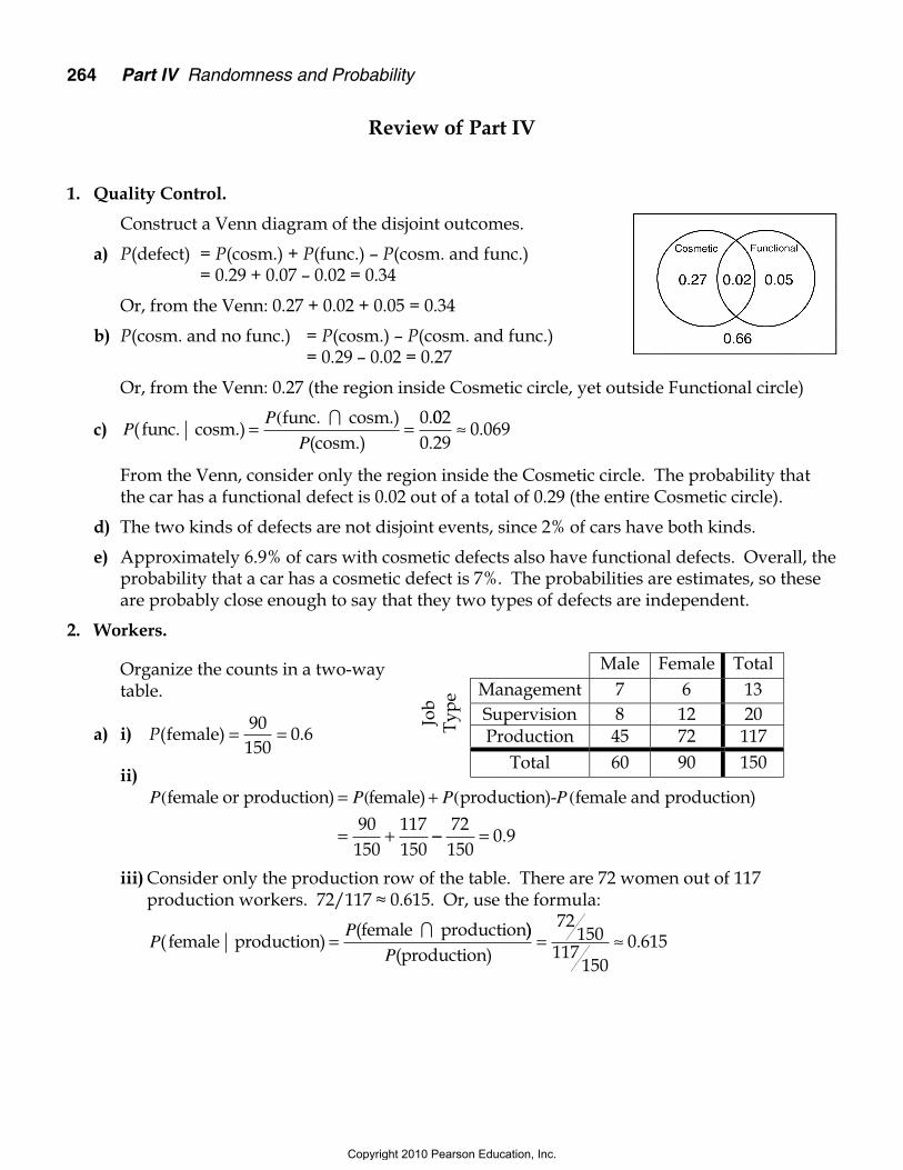
Construct a Venn diagram of the disjoint outcomes.

a) P(defect) = P(cosm.) + P(func.) – P(cosm. and func.)= 0.29 + 0.07 – 0.02 = 0.34

Or, from the Venn: 0.27 + 0.02 + 0.05 = 0.34

b) P(cosm. and no func.) = P(cosm.) – P(cosm. and func.)= 0.29 – 0.02 = 0.27

Or, from the Venn: 0.27 (the region inside Cosmetic circle, yet outside Functional circle)

c) PP

P( func. cosm.)

func. cosm.)(cosm.)

= =( .∩ 0 002

0 290 069

..≈

From the Venn, consider only the region inside the Cosmetic circle. The probability thatthe car has a functional defect is 0.02 out of a total of 0.29 (the entire Cosmetic circle).

d) The two kinds of defects are not disjoint events, since 2% of cars have both kinds.

e) Approximately 6.9% of cars with cosmetic defects also have functional defects. Overall, theprobability that a car has a cosmetic defect is 7%. The probabilities are estimates, so theseare probably close enough to say that they two types of defects are independent.

2. Workers.

Organize the counts in a two-waytable.

a) i) P( .female) = =90150

0 6

ii)P P P( ( (female or production) female) product= + iion)- female and production)P (

= +90150

117150

−− =72150

0 9.

iii) Consider only the production row of the table. There are 72 women out of 117production workers. 72/117 ≈ 0.615. Or, use the formula:

PP

( female production)(female production

=∩ ))

(production)P= ≈

72150

117150

0 615.

Male Female TotalManagement 7 6 13Supervision 8 12 20Jo

bTy

pe

Production 45 72 117Total 60 90 150

Copyright 2010 Pearson Education, Inc.

Review of Part IV 265

iv) Consider only the female column. There are 72 production workers out of a total of 90women. 72/90 = 0.8. Or, use the formula:

PP

(production female)(production female

=∩ ))

(female)P= =

72150

90150

0 8.

b) These data suggest that holding a production position may be associated with whether theworker is male or female.

60% of the plant employees are women, but 61.5% of the production workers are women.However, this is a small difference, and may be due to sampling error.

3. Airfares.

a) Let C = the price of a ticket to ChinaLet F = the price of a ticket to France.

Total price of airfare = 3C + 5F

b) µ = + = + = + =E C F E C E F( ) ( ) ( ) ( ) ( ) $3 5 3 5 3 1000 5 500 5500

σ = + = + = +SD C F Var C Var F( ) ( ( )) ( ( )) ( )3 5 3 5 3 1502 2 2 2 55 100 672 682 2( ) $ .≈

c) µ = − = − = − =E C F E C E F( ) ( ) ( ) $1000 500 500

σ = − = +SD C F Var C Var F( ) ( ) ( )

= + ≈150 100 180 282 2 $ .

d) No assumptions are necessary when calculating means. When calculating standarddeviations, we must assume that ticket prices are independent of each other for differentcountries but all tickets to the same country are at the same price.

4. Bipolar.

Let X = the number of people with bipolar disorder in a city of n = 10,000 residents.

These may be considered Bernoulli trials. There are only two possible outcomes, havingbipolar disorder or not having bipolar disorder. Psychiatrists estimate that the probabilitythat a person has bipolar is about 1 in 100, so p = 0.01. We will assume that the cases ofbipolar disorder are distributed randomly throughout the populations. The trials are notindependent, since the population is finite, but 10,000 people represent fewer than 10% ofall people. Therefore, the number of people with bipolar disorder in a city of 10,000 may bemodeled by Binom(10000, 0.01).

Since np = 100 and nq = 9900 are both greater than 10, Binom( , . )10000 0 01 may beapproximated by the Normal model, N(100, 9.95).

E X np( ) , ( . )= = =10 000 0 01 100 residents.

SD X npq( ) , ( . )( . ) .= = ≈10 000 0 01 0 99 9 95 residents.



We expect 100 city residents to have bipolar disorder. According to the Normal model, 200cases would be over 10 standard deviations above this mean. The probability of thisoccurring is essentially zero.

Technology can compute the probability according to the Binomial model. Again, theprobability that 200 cases of bipolar disorder exist in the city is essentially zero. We use theNormal model in this case, since it gives us a more intuitive idea of just how unlikely thisevent is.

5. A game.

a) Let X = net amount won

µ = = + − = −E X( ( . ) ( . ) ( . ) $ .) 0 0 10 2 0 40 2 0 50 0 20

σ 2 2 20 0 20 0 10 2 0 20 0= = − − + − −Var X( ) ( ( . )) ( . ) ( ( . )) ( .. ) ( ( . )) ( . ) .

( ) (

40 2 0 20 0 50 3 562+ − − − =

= =σ SD X Var X)) . $ .= ≈3 56 1 89

b) X + X = the total winnings for two plays.

µ

σ

= + = + = − + − = −

= + = +

= + ≈

E X X E X E X

SD X X Var X Var X

( ) ( ) ( ) ( . ) ( . ) $ .

( ) ( ) ( )

. . $ .

0 20 0 20 0 40

3 56 3 56 2 67

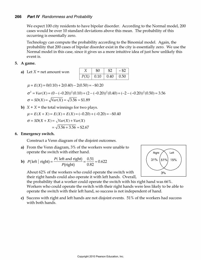
6. Emergency switch.


a) From the Venn diagram, 3% of the workers were unable tooperate the switch with either hand.

b) PP

P( left right)

left and right)(right)

= =( 0..

..

510 82

0 622≈

About 62% of the workers who could operate the switch withtheir right hands could also operate it with left hands. Overall,the probability that a worker could operate the switch with his right hand was 66%.Workers who could operate the switch with their right hands were less likely to be able tooperate the switch with their left hand, so success is not independent of hand.

c) Success with right and left hands are not disjoint events. 51% of the workers had successwith both hands.

X $0 $2 – $2P(X) 0.10 0.40 0.50



7. Twins.

The selection of these women can be considered Bernoulli trials. There are two possibleoutcomes, twins or no twins. As long as the women selected are representative of thepopulation of all pregnant women, then p = 1/90. (If the women selected arerepresentative of the population of women taking Clomid, then p = 1/10.) The trials arenot independent since the population of all women is finite, but 10 women are fewer than10% of the population of women.

Let X = the number of twin births from n = 10 pregnant women.

Let Y = the number of twin births from n = 10 pregnant women taking Clomid.

a) Use Binom(10, 1/90)P P( (at least one has twins) none have twi= −1 nns)

= − =

= −

1 0

1100

190

8990

0

P X( )

≈

10

0 106.

b) Use Binom(10, 1/10)P P( (at least one has twins) none have twi= −1 nns)

= − =

= −

1 0

1100

110

910

0

P Y( )

≈

10

0 651.

c) Use Binom(5, 1/90) and Binom(5, 1/90).

P P P( ( ( )

.

at least one has twins) no twins without Clomid) no twins with Clomid= −

= −

≈

1

150

190

8990

50

110

910

0 442

0 5 0 5

8. Deductible.

µ = = =E( ( . ) $ .cost) 500 0 005 2 50

σ 2 2 22 50 500 0 005 2 50 0 0= = − + −Var( ) ( . ) ( . ) ( . ) (cost .. ) .

( ) ( ) .

995 1243 75

1243 75

=

= = = ≈σ SD Varcost cost $$ .35 27

Expected (extra) cost of the cheaper policy with the deductible is $2.50, much less than the$12 surcharge for the policy with no deductible, so on average she will save money bygoing with the deductible. The standard deviation, at $35.27, is quite high compared to the$12 surcharge, indicating a high amount of variability. The value of the car shouldn’tinfluence the decision.



9. More twins.

In Exercise 7, it was determined that these were Bernoulli trials. Use Binom(5, 0.10).

Let X = the number of twin births from n = 5 pregnant women taking Clomid.

a) b)

P P X( ( )

( . ) ( . )

none have twins) = =

= ( )≈

0

0 1 0 950

0 5

00 590.

P P X( ( )

( . ) (

exactly one has twins) = =

= ( )1

0 151

1 00 9

0 328

4. )

.≈

c)P P X P( ( ) (at least three will have twins) = = +3 XX P X= + =

= ( ) + ( )4 5

0 1 0 9 0 1 053

54

3 2 4

) ( )

( . ) ( . ) ( . ) ( .99 0 1 0 9

0 00856

1 5 055

) ( . ) ( . )

.

+ ( )=

10. At fault.

If we assume that these drivers are representative of all drivers insured by the company,then these insurance policies can be considered Bernoulli trials. There are only twopossible outcomes, accident or no accident. The probability of having an accident isconstant, p = 0.005. The trials are not independent, since the populations of all drivers isfinite, but 1355 drivers represent fewer than 10% of all drivers. Use Binom(1355, 0.005).

a) Let X = the number of drivers who have an at-fault accident out of n = 1355.

E X np( ) , ( . ) .= = =1 355 0 005 6 775 drivers.

SD X npq( ) , ( . )( . ) .= = ≈1 355 0 005 0 995 2 60 drivers.

b) Since np = 6.775 < 10, the Normal model cannot be used to model the number of driverswho are expected to have accidents. The Success/Failure condition is not satisfied.

11. Twins, part III.

In Exercise 7, it was determined that these were Bernoulli trials. Use Binom(152, 0.10).

Let X = the number of twin births from n = 152 pregnant women taking Clomid.

a) E X np( ) ( . ) .= = =152 0 10 15 2 births.

SD X npq( ) ( . )( . ) .= = ≈152 0 10 0 90 3 70 births.

b) Since np = 15.2 and nq = 136.8 are both greater than 10, the Success/Failure condition issatisfied and Binom(152, 0.10) may be approximated by N(15.2, 3.70).



c) Using Binom(152, 0.10):P P X

P X P X

( ( )

( ) ( )

no more than 10) = ≤= = + + =

100 10…

== ( ) + + ( )1520

15210

0 10 0 90 0 100 152 10( . ) ( . ) ( . ) (… 00 90

0 097

142. )

.≈

According to the Binomial model, the probability that no more than 10 women would havetwins is approximately 0.097.

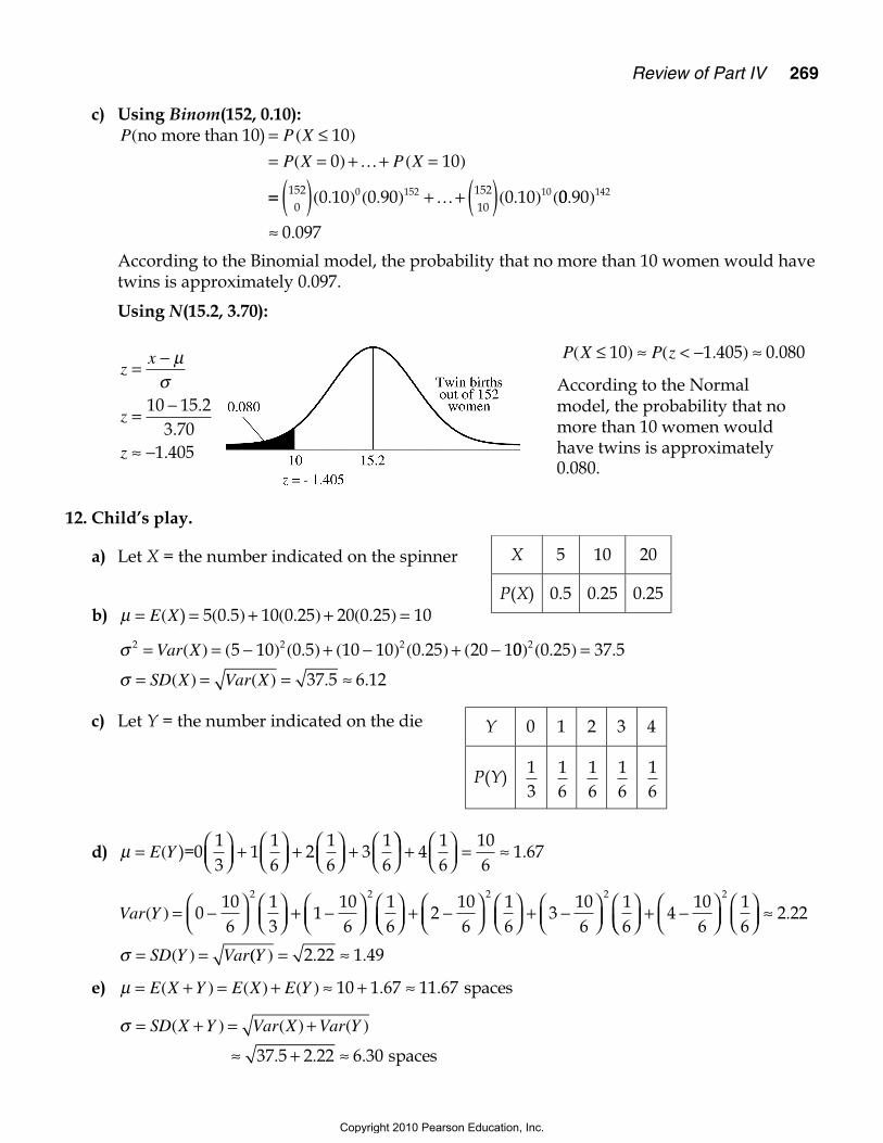
Using N(15.2, 3.70):

12. Child’s play.

a) Let X = the number indicated on the spinner

b) µ = = + + =E X( ( . ) ( . ) ( . )) 5 0 5 10 0 25 20 0 25 10

σ 2 2 25 10 0 5 10 10 0 25 20 1= = − + − + −Var X( ) ( ) ( . ) ( ) ( . ) ( 00 0 25 37 5

37 5 6 12

2) ( . ) .

( ) ( ) . .

=

= = = ≈σ SD X Var X

c) Let Y = the number indicated on the die

d) µ =

+

+

+

E Y( )=013

116

216

316

+

= ≈416

106

1 67.

Var Y( ) = −

+ −

0106

13

1106

16

2 2

+ −

+ −

2106

16

3106

16

2 2

+ −

≈

= =

4106

16

2 222

.

( )σ SD Y Var(( ) . .Y = ≈2 22 1 49

e) µ = + = + ≈ + ≈E X Y E X E Y( ) ( ) ( ) . .10 1 67 11 67 spaces

σ = + = +SD X Y Var X Var Y( ) ( ) ( )

spaces≈ + ≈37 5 2 22 6 30. . .

X 5 10 20

P(X) 0.5 0.25 0.25

Y 0 1 2 3 4

P(Y) 13

16

16

16

16

zx

z

z

= −

= −

≈ −

µσ

10 15 23 70

1 405

..

.

According to the Normalmodel, the probability that nomore than 10 women wouldhave twins is approximately0.080.

P X P z( ) ( . ) .≤ ≈ < − ≈10 1 405 0 080



13. Language.

Assuming that the freshman composition class consists of 25 randomly selected people,these may be considered Bernoulli trials. There are only two possible outcomes, having aspecified language center or not having the specified language center. The probabilities ofthe specified language centers are constant at 80%, 10%, or 10%, for right, left, and two-sided language center, respectively. The trials are not independent, since the population ofpeople is finite, but we will select fewer than 10% of all people.

a) Let L = the number of people with left-brain language control from n = 25 people.

Use Binom(25, 0.80).

P P L

P L P L

( ( )

( ) ( )

no more than 15) = ≤= = + + =

150 15…

==( ) + + ( )250

2515

0 80 0 20 0 80 0 20 25 15( . ) ( . ) ( . ) ( .… 00

0 0173

10)

.≈According to the Binomial model, the probability that no more than 15 students in a classof 25 will have left-brain language centers is approximately 0.0173.

b) Let T = the number of people with two-sided language control from n = 5 people.

Use Binom(5, 0.10).

P P T( (none have two-sided language control) = ==

= ( )≈

0

0 10 0 90

0 590

50

0 5

)

( . ) ( . )

.

c) Use Binomial models:

E np

E nL( ( . )

(

left) peopleright)

= = ==

1200 0 80 960pp

E npR

T

= =− = =

1200 0 10 1201

( . )

( )

peopletwo sided 2200 0 10 120( . ) = people

d) Let R = the number of people with right-brain language control.

E R npR( ) ( . )= = =1200 0 10 120 people

SD R np qR R( ) ( . )( . ) .= = ≈1200 0 10 0 90 10 39 people.



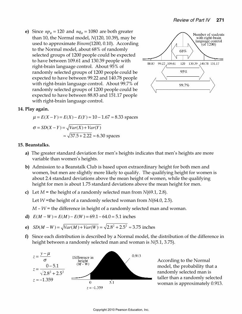
e) Since npR = 120 and nqR = 1080 are both greaterthan 10, the Normal model, N(120, 10.39), may beused to approximate Binom(1200, 0.10). Accordingto the Normal model, about 68% of randomlyselected groups of 1200 people could be expectedto have between 109.61 and 130.39 people withright-brain language control. About 95% ofrandomly selected groups of 1200 people could beexpected to have between 99.22 and 140.78 peoplewith right-brain language control. About 99.7% ofrandomly selected groups of 1200 people could beexpected to have between 88.83 and 151.17 peoplewith right-brain language control.

14. Play again.

µ = − = − ≈ − ≈E X Y E X E Y( ) ( ) ( ) . .10 1 67 8 33 spaces

σ = − = +SD X Y Var X Var Y( ) ( ) ( )

spaces≈ + ≈37 5 2 22 6 30. . .

15. Beanstalks.

a) The greater standard deviation for men’s heights indicates that men’s heights are morevariable than women’s heights.

b) Admission to a Beanstalk Club is based upon extraordinary height for both men andwomen, but men are slightly more likely to qualify. The qualifying height for women isabout 2.4 standard deviations above the mean height of women, while the qualifyingheight for men is about 1.75 standard deviations above the mean height for men.

c) Let M = the height of a randomly selected man from N(69.1, 2.8).

Let W =the height of a randomly selected woman from N(64.0, 2.5).

M – W = the difference in height of a randomly selected man and woman.

d) E M W E M E W( ) ( ) ( ) . . .− = − = − =69 1 64 0 5 1 inches

e) SD M W Var M Var W( ) ( ) ( ) . . .− = + = + ≈2 8 2 5 3 752 2 inches

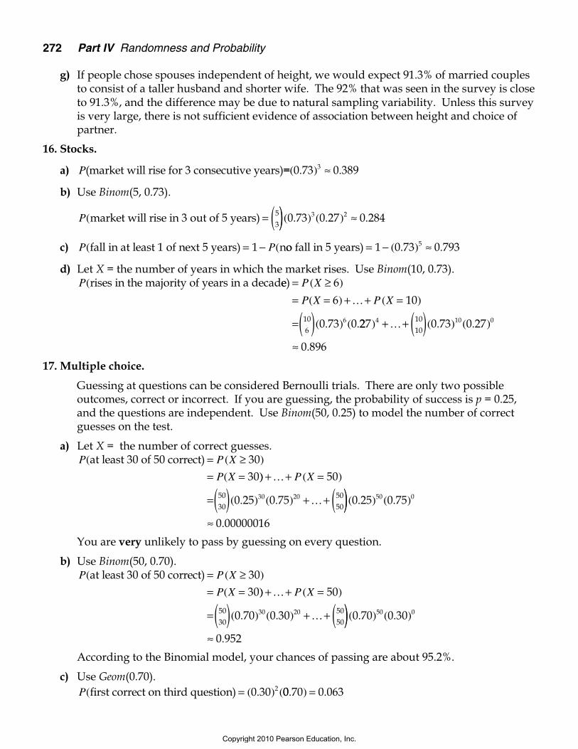
f) Since each distribution is described by a Normal model, the distribution of the difference inheight between a randomly selected man and woman is N(5.1, 3.75).

zy

z

z

=−

=−

+≈ −

µσ

0 5 1

2 8 2 51 359

2 2

.

. ..

According to the Normalmodel, the probability that arandomly selected man istaller than a randomly selectedwoman is approximately 0.913.



g) If people chose spouses independent of height, we would expect 91.3% of married couplesto consist of a taller husband and shorter wife. The 92% that was seen in the survey is closeto 91.3%, and the difference may be due to natural sampling variability. Unless this surveyis very large, there is not sufficient evidence of association between height and choice ofpartner.

16. Stocks.

a) P(market will rise for 3 consecutive years)==( . ) .0 73 0 3893 ≈

b) Use Binom(5, 0.73).

P(market will rise in 3 out of 5 years) = (53)) ≈( . ) ( . ) .0 73 0 27 0 2843 2

c) P P( (fall in at least 1 of next 5 years) n= −1 oo fall in 5 years) = − ≈1 0 73 0 7935( . ) .

d) Let X = the number of years in which the market rises. Use Binom(10, 0.73).P(rises in the majority of years in a decadee) = ≥

= = + + =

=( )P X

P X P X

( )

( ) ( )

( . ) ( .

66 10

0 73 0106

6

…

227 0 73 0 27

0 896

4 10 01010

) ( . ) ( . )

.

+ + ( )≈

…

17. Multiple choice.

Guessing at questions can be considered Bernoulli trials. There are only two possibleoutcomes, correct or incorrect. If you are guessing, the probability of success is p = 0.25,and the questions are independent. Use Binom(50, 0.25) to model the number of correctguesses on the test.

a) Let X = the number of correct guesses.P P X

P X

( ( )

(

at least 30 of 50 correct) = ≥= =

3030)) ( )

( . ) ( . )

+ + =

=( ) + + (…

…

P X 50

0 25 0 755030

5050

30 20 ))≈

( . ) ( . )

.

0 25 0 75

0 00000016

50 0

You are very unlikely to pass by guessing on every question.

b) Use Binom(50, 0.70).P P X

P X

( ( )

(

at least 30 of 50 correct) = ≥= =

3030)) ( )

( . ) ( . )

+ + =

=( ) + + (…

…

P X 50

0 70 0 305030

5050

30 20 ))≈

( . ) ( . )

.

0 70 0 30

0 952

50 0

According to the Binomial model, your chances of passing are about 95.2%.

c) Use Geom(0.70).P( ( . ) (first correct on third question) = 0 30 2 00 70 0 063. ) .=



18. Stock strategy.

a) This does not confirm the advice. Stocks have risen 75% of the time after a two-year fall,but there have only been eight occurrences of the two-year fall. The sample size is verysmall, and therefore highly variable.

b) Stocks have actually risen in 73% of years. This is not much different from the strategy ofthe advisors, which yielded a rise in 75% of years (from a very small sample of years.)

19. Insurance.

The company is expected to pay $100,000 only 2.6% of the time, while always gaining $520from every policy sold. When they pay, they actually only pay $99,480.

E(profit) = $520(0.974) – $99,480(0.026) = – $2,080.

The expected profit is actually a loss of $2,080 per policy. The company had better raise itspremiums if it hopes to stay in business.

20. Teen smoking.

Randomly selecting high school students can be considered Bernoulli trials. There are onlytwo possible outcomes, smoker or nonsmoker. The probability that a student is a smoker isp = 0.30. The trials are not independent, since the population is finite, but we are notsampling more than 10% of all high school students.

a) P( ( . )none of the first 4 are smokers) = =0 7 04 ..2401

b) Use Geom(0.3).P( ( . ) (first smoker is the sixth person) = 0 7 5 00 3 0 050. ) .≈

c) Use Binom(10, 0.3). Let X = the number of smokers among n = 10 students.P P X

P X

( ( )

(

no more than 2 smokers of 10) = ≤= =

200 1 2

0 30 0 70100

101

0 10

) ( ) ( )

( . ) ( . )

+ = + =

=( ) + (P X P X

)) + ( )≈

( . ) ( . ) ( . ) ( . )

.

0 30 0 70 0 30 0 70

0 383

1 9 2 8102

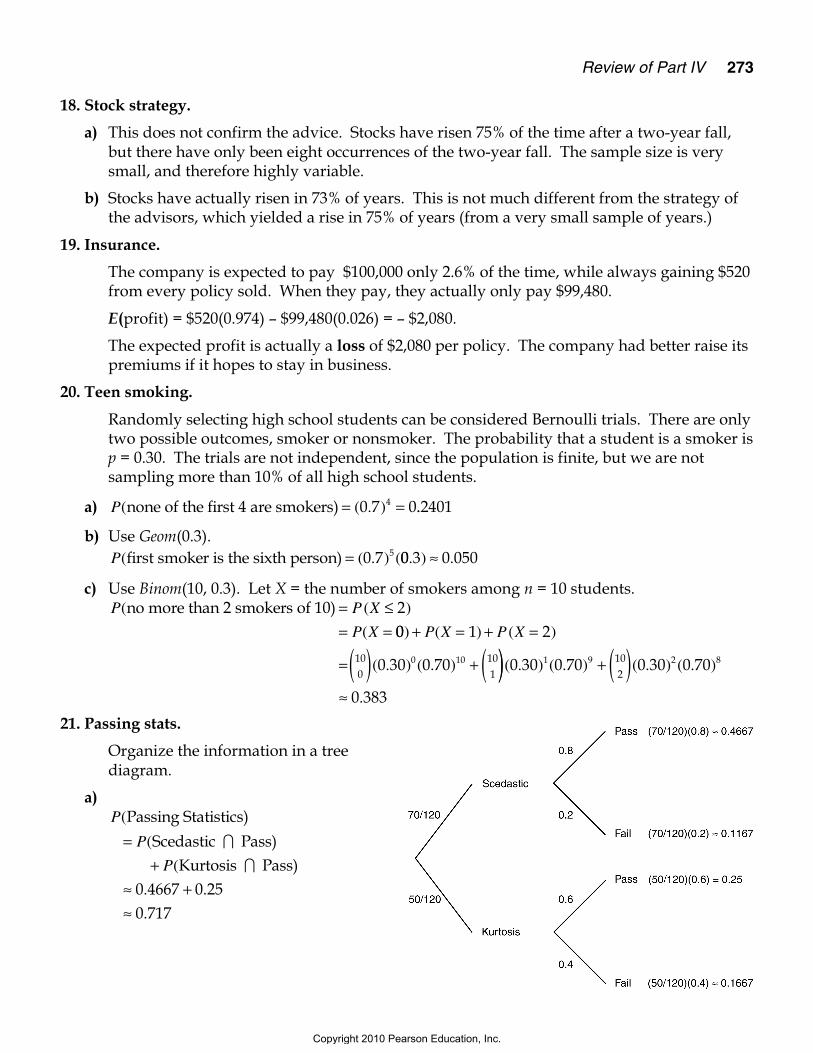
21. Passing stats.

Organize the information in a treediagram.

a)P

P

(

(

Passing Statistics) Scedastic Pass)= ∩ Kurtosis Pass)

+≈ +

P(

. .

∩0 4667 0 25

≈ 0 717.



b)P

P

P

(Kurtosis Fail)

Kurtosis Fail)

(Fai=

( ∩ll)

≈+

≈0 1667

0 1167 0 16670 588

.

. ..

22. Teen smoking II.

In Exercise 22, it was determined that the selection of students could be considered to beBernoulli trials.

a) Use Binom(120, 0.30) to model the number of smokers out of n = 120 students.E np( ) ( . )number of smokers smoker= = =120 0 30 36 ss.

b) SD npq( ) ( . )( . )number of smokers = = ≈120 0 30 0 70 5..02 smokers.

c) Since np = 36 and nq = 84 are both greater than 10, the Success/Failure condition is satisfiedand Binom(120, 0.30) may be approximated by N(36, 5.02).

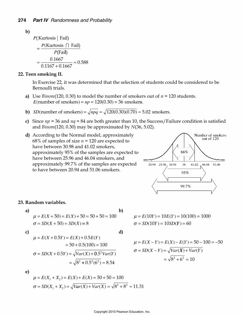
d) According to the Normal model, approximately68% of samples of size n = 120 are expected tohave between 30.98 and 41.02 smokers,approximately 95% of the samples are expected tohave between 25.96 and 46.04 smokers, andapproximately 99.7% of the samples are expectedto have between 20.94 and 51.06 smokers.

23. Random variables.

a) b)µσ

= + = + = + == + =

E X E X

SD X SD X

( ) ( )

( ) ( )

50 50 50 50 10050 == 8

µσ

= = = == =

E Y E Y

SD Y SD

( ) ( ) ( )

( ) (

10 10 10 100 100010 10 YY ) = 60

c) d)µ = + = +E X Y E X E Y( . ) ( ) . ( )0 5 0 5 = + =

= + = +

50 0 5 100 100

0 5

. ( )

( . ) ( )σ SD X Y Var X 00 5

8

2

2

. ( )Var Y

= ++ ≈0 5 6 8 542 2. ( ) .

µ

σ

= − = − = − = −

= − =

E X Y E X E Y

SD X Y Var

( ) ( ) ( )

( ) (

50 100 50

XX Var Y) ( )+

= + = 8 6 102 2

e)µ

σ

= + = + = + =

= + =

E X X E X E X

SD X X V

( ) ( ) ( )

( )

1 2

1 2

50 50 100

aar X Var X( ) ( ) .+ = + ≈8 8 11 312 2



24. Merger.

Small companies may run in to trouble in the insurance business. Even if the expectedprofit from each policy is large, the profit is highly variable. There is a small chance that acompany would have to make several huge payouts, resulting in an overall loss, not aprofit. By combining two small companies together, the company takes in profit frommore policies, making the larger company more resistant to the possibility of a largepayout. This is because the total profit is increasing by the expected profit from eachadditional policy, but the standard deviation is increasing by the square root of the sum ofthe variances. The larger a company gets, the more the expected profit outpaces thevariability associated with that profit.

25. Youth survey.

a) Many boys play computer games and use email, so the probabilities can total more than100%. There is no evidence that there is a mistake in the report.

b) Playing computer games and using email are not disjoint. If they were, the probabilitieswould total 100% or less.

c) Emailing friends and being a boy or girl are not independent. 76% of girls emailed friendsin the last week, but only 65% of boys emailed. If emailing were independent of being aboy or girl, the probabilities would be the same.

d) Let X = the number of students chosen until the first student is found who does not use theInternet. Use Geom(0.07). P X( ) ( . ) ( . ) .= = ≈5 0 93 0 07 0 05244 .

26. Meals.

Let X = the amount the student spends daily.

a) µ = + = + = + =E X X E X E X( ) ( ) ( ) . . $ .13 50 13 50 27 00

σ = + = +SD X X Var X Var X( ) ( ) ( )

= + ≈7 7 9 902 2 $ .

b) In order to calculate the standard deviation, we must assume that spending on differentdays is independent. This is probably not valid, since the student might tend to spend lesson a day after he has spent a lot. He might not even have money left to spend!

c) µ = + + + + + + = = =E X X X X X X X E X( ) ( ) ($ . ) $ .7 7 13 50 94 50

σ = + + + + + +

= + + +

SD X X X X X X X

Var X Var X Var X Va

( )

( ) ( ) ( ) rr X Var X Var X Var X( ) ( ) ( ) ( )

( ) $ .

+ + +

= ≈7 7 18 522

d) Assuming once again that spending on different days is independent, it is unlikely that thestudent will spend less than $50. This level of spending is about 2.4 standard deviationsbelow the weekly mean. Don’t try to approximate the probability! We don’t know theshape of this distribution.



27. Travel to Kyrgyzstan.

a) If you spend an average of 4237 soms per day, you can stay about 90 0004237

21,

≈ days .

b) Assuming that your daily spending is independent, the standard deviation is the squareroot of the sum of the variances for 21 days.

σ = ≈21 360 1649 732( ) . soms

c) The standard deviation in your total expenditures is about 1650 soms, so if you don’t thinkyou will exceed your expectation by more than 2 standard deviations, bring an extra 3300soms. This gives you a cushion of about 157 soms for each of the 21 days.

28. Picking melons.

a) µ = − = − = − =E E E( ) ( ) ( )First Second First Second 22 18 44 lbs.

b) σ = − = + =SD Var Var( ) ( ) ( )First Second First Second 2.. .5 2 3 202 2+ ≈ lbs.

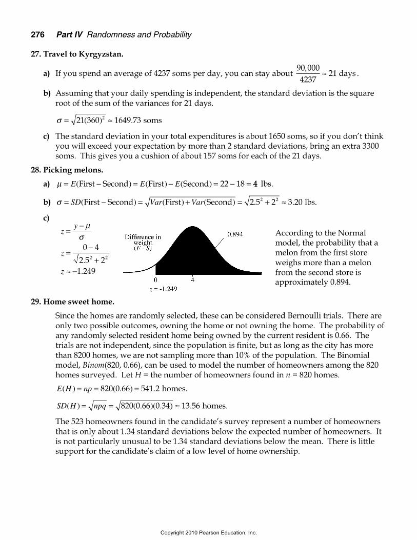
c)

29. Home sweet home.

Since the homes are randomly selected, these can be considered Bernoulli trials. There areonly two possible outcomes, owning the home or not owning the home. The probability ofany randomly selected resident home being owned by the current resident is 0.66. Thetrials are not independent, since the population is finite, but as long as the city has morethan 8200 homes, we are not sampling more than 10% of the population. The Binomialmodel, Binom(820, 0.66), can be used to model the number of homeowners among the 820homes surveyed. Let H = the number of homeowners found in n = 820 homes.

E H np( ) ( . ) .= = =820 0 66 541 2 homes.

SD H npq( ) ( . )( . ) .= = ≈820 0 66 0 34 13 56 homes.

The 523 homeowners found in the candidate’s survey represent a number of homeownersthat is only about 1.34 standard deviations below the expected number of homeowners. Itis not particularly unusual to be 1.34 standard deviations below the mean. There is littlesupport for the candidate’s claim of a low level of home ownership.

zy

z

z

=−

=−

+≈ −

µσ

0 4

2 5 21 249

2 2..

According to the Normalmodel, the probability that amelon from the first storeweighs more than a melonfrom the second store isapproximately 0.894.



30. Buying melons.

The mean price of a watermelon at the first store is 22(0.32) = $7.04.At the second store the mean price is 18(0.25) = $4.50.The difference in the price of the watermelons is expected to be $7.04 – $4.50 = $2.54.

The standard deviation in price at the first store is 2.5(0.32) = $0.80.At the second store, the standard deviation in price is 2(0.25) = $0.50.

The standard deviation of the difference is 0 80 0 50 0 942 2. . $ . .+ ≈

31. Who’s the boss?

a) P( ( . ) .first three owned by women) = ≈0 26 0 0183

b) P(none of the first four are owned by women)) = ≈( . ) .0 74 0 3004

c) P(sixth firm called is owned by women none of the first five were) = 0 26.

Since the firms are chosen randomly, the fact that the first five firms were owned by menhas no bearing on the ownership of the sixth firm.

32. Jerseys.

a) P(all four kids get the same color) =

414

≈4

0 0156.

(There are four different ways for this to happen, one for each color.)

b) P( .all four kids get white) =

≈14

0 00394

c) P(all four kids get white) =

16

14

33

0 0026≈ .

33. When to stop?

a) Since there are only two outcomes, 6 or not 6, the probability of getting a 6 is 1/6, and thetrials are independent, these are Bernoulli trials. Use Geom(1/6).

µ = = =1 1

16

6p

rolls

b) If 6’s are not allowed, the mean of each die roll is 1 2 3 4 5

53

+ + + += . You would expect to

get 15 if you rolled 5 times.

c) P( .5 rolls without a 6) =

≈56

0 4025



34. Plan B.

a) If 6’s are not allowed, the mean of each die roll is 1 2 3 4 5

53

+ + + += .

b) Let X = your current score. You expect to lose it all 16

of the time, so your expected loss per

roll is 16

X.

c) Expected gain equals expected loss when 16

3X = . So, X = 18.

d) Roll until you get 18 points, then stop.

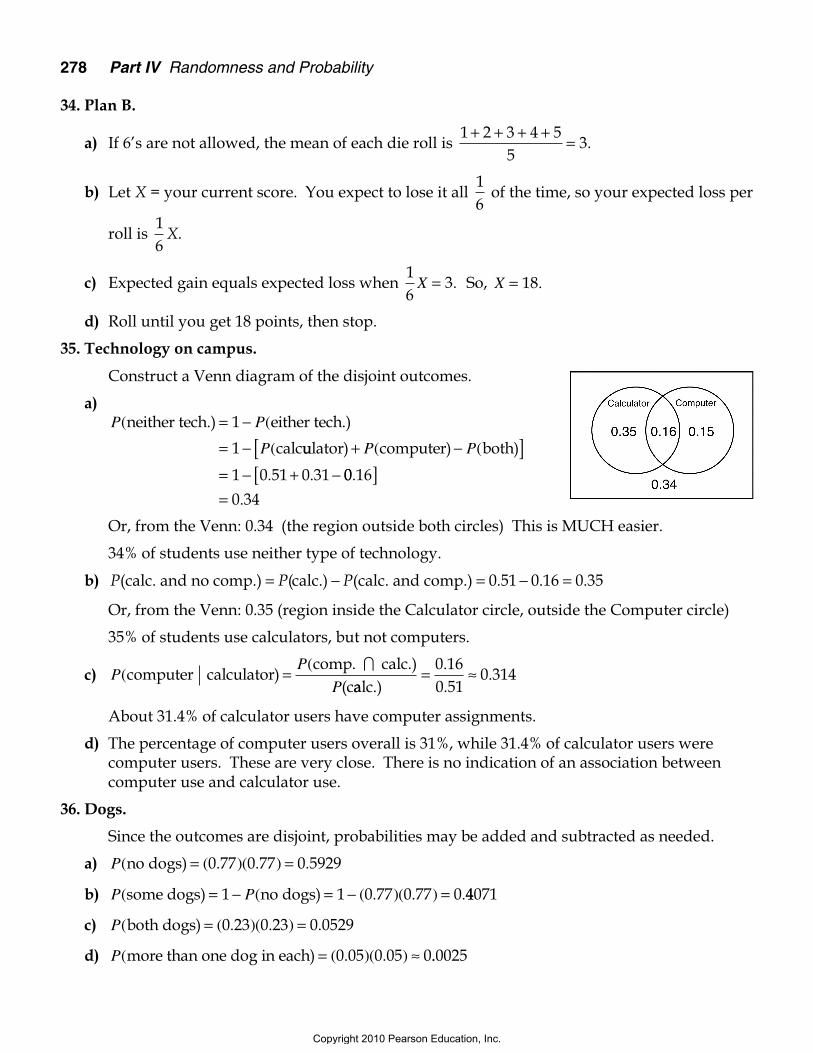
35. Technology on campus.


a)P P

P

( (

(

neither tech.) either tech.)

calc

= −

= −

1

1 uulator) computer) both)+ −[ ]= − + −

P P( (

. .1 0 51 0 31 00 160 34

.

.

[ ]=

Or, from the Venn: 0.34 (the region outside both circles) This is MUCH easier.

34% of students use neither type of technology.

b) P P P( ( ( . . .calc. and no comp.) calc.) calc. and comp.)= − = − =0 51 0 16 0 35

Or, from the Venn: 0.35 (region inside the Calculator circle, outside the Computer circle)

35% of students use calculators, but not computers.

c) PP

P(

(computer calculator)

comp. calc.)(c

=∩

aalc.)= ≈

0 160 51

0 314.

..

About 31.4% of calculator users have computer assignments.

d) The percentage of computer users overall is 31%, while 31.4% of calculator users werecomputer users. These are very close. There is no indication of an association betweencomputer use and calculator use.

36. Dogs.

Since the outcomes are disjoint, probabilities may be added and subtracted as needed.

a) P( ( . )( . ) .no dogs) = =0 77 0 77 0 5929

b) P P( ( ( . )( . ) .some dogs) no dogs)= − = − =1 1 0 77 0 77 0 44071

c) P( ( . )( . ) .both dogs) = =0 23 0 23 0 0529

d) P( ( . )( . )more than one dog in each) = ≈0 05 0 05 0..0025



37. Socks.

Since we are sampling without replacement, use conditional probabilities throughout.

a) P(2 blue) =

= =4

12311

12132

111

b) P(no grey) =

= =712

611

42132

722

c) P P( (at least one black) no black)= − = −

1 1912

= =811

60132

511

d) P(green) = 0 (There aren’t any green socks in the drawer.)

e) P P P P( ( ( (match) 2 blue) 2 grey) 2 black)= + + =4

12

+

+

311

512

411

312

=211

1966

38. Coins.

Coin flips are Bernoulli trials. There are only two possible outcomes, the probability ofeach outcome is constant, and the trials are independent.

a) Use Binom(36, 0.5). Let H = the number of heads in n = 36 flips.

µ = = = =E H np( ) ( . )36 0 5 18 heads.

σ = = = =SD H npq( ) ( . )( . )36 0 5 0 5 3 heads.

b) Two standard deviations above the mean corresponds to 6 “extra” heads observed.

c) The standard deviation of the number of heads when 100 coins are flipped isσ = = =npq 100 0 5 0 5 5( . )( . ) heads. Getting 6 “extra” heads is not unusual.

d) Following the “two standard deviations” measurement, 10 or more “extra” heads would beunusual.

e) What appears surprising in the short run becomes expected in a larger number of flips.The “Law of Averages” is refuted, because the coin does not compensate in the long run.A coin that is flipped many times is actually less likely to show exactly half heads than acoin flipped only a few times. The Law of Large Numbers is confirmed, because thepercentage of heads observed gets closer to the percentage expected due to probability.

39. The Drake equation.

a) N fp⋅ represents the number of stars in the Milky Way Galaxy expected to have planets.

b) N f n fp e i⋅ ⋅ ⋅ represents the number of planets in the Milky Way Galaxy expected to haveintelligent life.

c) f fl i⋅ is the probability that a planet has a suitable environment and has intelligent life.



d) f Pl = (life suitable environment). This is the probability that life develops, if a planet has asuitable environment.

f Pi = (intelligence life). This is the probability that the life develops intelligence, if aplanet already has life.

f Pc = (communication intelligence). This is the probability that radio communicationdevelops, if a planet already has intelligent life.

40. Recalls.

Organize the information in a tree diagram.

a)P P( (recall) American recall)

= Japanese recall)

++

P

P

(

((

. .

German recall) = +0 014 0 002 ++

=0 001

0 017.

.

b)

PP

P(

(

(American recall)

American recall)r

=∩

eecall)

=+ +

≈

0 0140 014 0 002 0 001

0 824

.

. . .

.

41. Pregnant?

Organize the information in a treediagram.

P

P

(

(

pregnant positive test)

pregnant

=∩ ppositive test)

positive test)

P(

.

.=

0 6860 6886 0 006

0 991

+

≈

.

.



42. Door prize.

a) The probability that the first person in line wins is 1 out of 100, or 0.01.

b) If you are third in line, the two people ahead of you must not win in order for you to win.The probability is (0.99)(0.99)(0.01) = 0.009801.

c) There must be 100 losers in a row. The probability is ( . ) . .0 99 0 366100 ≈

d) The first person in line has the greatest chance of winning at p = 0.01. The probability ofwinning decreases from there, since winning is dependent upon everyone else in front ofyou in line losing.

e) Position is irrelevant now. Everyone has the same chance of winning, p = 0.01. One way tovisualize this is to imagine that one ball is handed out to each person. Only one person outof the 100 people has the red ball. It might be you!

If you insist that the probabilities are still conditional, since you are sampling withoutreplacement, look at it this way:

Consider P(sixth person wins) =

99100

9899

97798

9697

9596

195

110

=00


Documents

Review of Part IV - Weebly · Review of Part IV 265 iv)Consider only the female column.There are 72 production workers out of a total of 90 women. 72/90 = 0.8. Or, …