REVIEW OF SEISMIC REFLECTION - unn.edu.ng Abraham.pdf · Migration 36 ... GENERAL INTRODUCTION 1.1. Introduction Seismic reflection method is the most commonly used geophysical technique

1

Digitally Signed by: Content manager’s Name

DN : CN = Weabmaster’s name

O= University of Nigeria, Nsukka

OU = Innovation Centre

Ugwoke Oluchi C.

FACULTY OF PHYSICAL SCIENCES

DEPARTMENT OF PHYSICS AND ASTRONOMY

REVIEW OF SEISMIC REFLECTION

IBEKWE, ABRAHAM IKECHUKWU

(PG/M.Sc/09/51925)

2

REVIEW OF SEISMIC REFLECTION OPERATIONS

BY

IBEKWE, ABRAHAM IKECHUKWU

(PG/M.Sc/09/51925)

A PROJECT

SUBMITTED TO THE DEPARTMENT OF PHYSICS AND ASTRONOMY,

FACULTY OF PHYSICAL SCIENCES,

UNIVERSITY OF NIGERIA, NSUKKA,

IN PARTIAL FULFILMENT FOR THE AWARD OF MASTER OF SCIENCES (M.Sc)

IN SOLID EARTH GEOPHYSICS.

SUPERVISORS

PROF. F. N. OKEKE (FAS)

DR. J. U. CHUKUDEBELU

NOVEMBER, 2013

3

CERTIFICATION

This is to certify that this project was submitted by Ibekwe, A. Ikechukwu to and approved by the

Department of Physics and Astronomy, Faculty of Physical Sciences, University of Nigeria,

Nsukka, in partial fulfillment for the award of Master of Sciences (M.Sc) in Solid Earth

Geophysics.

__________________________________________ _______________

Head of Department Date

__________________________________________ ______________

Supervisor Date

__________________________________________ ______________

Supervisor Date

4

ACKNOWLEDGEMENT

“Dreams are not the things you see when you sleep. Dreams are those things that keep you from

sleep!”

The completion of this project is a dream come true and I would like to acknowledge all those who

in one way or another contributed to this great success.

Firstly, I would like to acknowledge the Head, staff and students of the Department of Physics and

Astronomy, UNN, for the knowledge and time we shared. Your inputs actually contributed to my

success. Most especially my supervisors, Prof (Mrs.) F. N. Okeke (the most compatible person I

have ever worked with) and Dr. J. U. Chukudebelu (if I were to have a second dad, it would be him)

for their patience and constructive criticism towards me and my work.

I also acknowledge my family for their unalloyed and unreserved support towards my education. I

want to specifically observe my mum, Mrs. N. N. Ibekwe (the best mum in the world) and Engr.

Nelson Uzonwa and his family for investing in me. Your efforts have finally paid off.

To my course mates, Chimaroke, Chisom and Robert. You guys are the best.

I also want to appreciate Mrs. Ijeomakanu. She surprised me sometime.

To all my friends, Cyril, Iyke Allah, Victor (76), Salata and Chinenye. I love you all!

5

DEDICATION

This work is dedicated to all those who believe in me, most especially, my mum and sisters.

And also to my future kids!

6

ABSTRACT

In the summer of 1921, a small team of physicists and geologists (William P. Haseman, J. Clarence

Karcher, Irving Perrine, and Daniel W. Ohern) performed a historical experiment near the Vines

Branch area in south-central Oklahoma using a dynamite charge as a seismic source and a special

instrument called a seismograph. The team recorded seismic waves that had traveled through the

subsurface of the earth. Analysis of the recorded data revealed seismic reflections from a boundary

between two underground rock layers.

Further analysis of the data produced an image of the subsurface, called a seismic reflection profile

that agreed with a known geologic feature. That result is widely regarded as the first proof that an

accurate image of the earth's subsurface could be made using reflected seismic waves.

Since that day till date, more technological and developmental advancements have been recorded in

the geophysical sphere the world over. Today, reflection seismology is a thriving business with the

result of the 1921 experiment being nothing compared to present day survey results.

This review attempts to take a critical look at some seismic reflection operations that have been

performed around the world, analyze the approach employed in the acquisition, processing and

interpretation of seismic data and to suggest or recommend suitable and more appropriate approaches

to specific survey objectives.

This review work begins by introducing the basic concepts and principles upon which seismic

reflection work operates, and then will take a look at seismic data acquisition methods and the basic

processes applied in transforming a noise-filled data to an output with clearer features (data

processing). Ten (10) seismic reflection cases will be reviewed. The review will cover their

7

acquisition, processing and interpretation procedures and their results discussed. This project will

conclude by proffering recommendations as to what method or sequence a seismic crew could adopt

to address a desired result.

8

TABLE OF CONTENT

TITLE PAGE i

CERTIFICATION ii

ACKNOWLEDGEMENT iii

DEDICATION iv

ABSTRACT v

TABLE OF CONTENT vii

LIST OF FIGURES xi

LIST OF TABLES xii

CHAPTER ONE: GENERAL INTRODUCTION

1.1 Introduction 1

1.2 Elasticity Theory 2

1.3 Stress 2

1.4 Strain 4

1.5 Seismic Wave Equation 6

1.6 Seismic Waves 9

1.6.1 Body Waves 10

1.6.2 Surface Waves 11

1.7 Seismic Wave Propagation 11

1.7.1 Huygen’s Principle 12

1.7.2 Fermat’s Principle 12

1.8 Wave Attenuation 12

1.9 Seismic Velocity 13

1.10 Factors that Affect Seismic Velocity 14

1.11 Purpose of Study 14

CHAPTER TWO: SEISMIC DATA ACQUISITION AND PROCESSING

9

2.1 Introduction 15

2.2 Seismic Data Acquisition 15

2.3 Seismic Data Processing 16

2.4 Pre-Processing 17

2.4.1. Demultiplexing 17

2.4.2 Trace Editing and Muting 19

2.4.3 Gain Recovery 19

2.5. Main Processing 21

2.5.1. Deconvolution 22

2.5.2. CMP Sorting 25

2.5.3. Velocity Analysis 26

2.5.4. NMO Correction 29

2.5.5. Dip move-out (DMO) Correction 30

2.5.6. Statics Corrections 32

2.5.7 Residual Statics Correction (RSC) 34

2.5.8. Stacking 35

2.5.9. Digital Filtering 35

2.5.10. Migration 36

2.6. Mathematical Operations in Seismic Data Processing 40

2.6.1. The Fourier Series/Transform 40

2.6.2. Convolution 44

2.6.3. Correlation 46

2.6.4. The z-transform 47

CHAPTER THREE: LITERATURE REVIEW

3.1. Introduction 49

3.2. Case 1: Seismic Reflection Studies in the Skellefte

10

Ore District, Northern Sweden 50

3.3. Case 2: Seismic Reflection Tomography: A Case

Study of a Shallow Lake in Lake Balaton 53

3.4. Case 3: COCORP’S Deep Seismic Reflection Profiling in

the Williston Basin (Comparison of Explosive and

Vibroseis Source Energy Penetration) 57

3.5. Case 4: Reflection Seismic and Ground-Penetrating

Radar Study of -Previously Mined (Lead/Zinc) Ground,

Joplin, Missouri 61

3.6. Case 5: Seismic Processing and Velocity Assessments

in the Oil and Gas Resource Potential of the 1002 AREA,

Arctic National Wild Life Refuge (ANWR), Alaska 64

3.7. Case 6: Seismic Reflection Investigation of C-1 to F-1

Sector of the Superconducting Super Collider (SSC)

Ring West of Waxahachie, Texas 65

3.8. Case 7: Analysis of Existing Seismic Reflection Data in

South Florida for Aquifer Storage and Recovery (ASR)

Regional Study 71

3.9. Case 8: 4D Acquisition Using Two Boats in the Enfield

Oil Field Offshore, Western Australia 72

3.10. Case 9: 3D Interpretation of The Espoir Field Area,

Offshore Ivory Coast 76

3.11 Case 10: Structural and Stratigraphic Mapping of

Emi field, offshore Niger Delta, Nigeria. 78

CHAPTER FOUR: RESULT DISCUSSION

4.1. Results of Case 1 82

4.2. Results for Case 2 84



11







CHAPTER FIVE: DISCUSSIONS AND CONCLUSIONS

5.1. Discussions and Conclusions 97

5.3. Recommendation 99

REFERENCES 101

12

LIST OF FIGURES

Fig. 1.1: Components of stress acting on faces perpendicular to the x-axis. 3

Fig 2.1: Conventional seismic data processing flowchart 18

Fig 2.2 A stacking chart showing traces and common gathers 26

Fig 2.3: A CMP gather (a) containing a single event with a move-out velocity of

2264m/s; (b) shows NMO correction of (a) using appropriate velocity

(2264m/s); (c) shows an over-corrected event because a very low velocity

was used (2000m/s) and (d) shows under-correction resulting from too

high a velocity (2500m/s). 31

Fig 2.4: Illustration of elevation statics 33

Fig 2.5: Design and application of zero-phase filter in the frequency domain 38

Fig 2.6: Design and application of zero-phase filter in the time domain 38

Fig 3.1:Bedrock geological map of the Kristineberg area, with the locations

of the seismic profiles, the CDP lines and the temporary seismic stations 51

Fig 3.2: Location map of the broader study area of Lake Balaton 54

Fig 3.3. A map showing the survey area of the Williston basin and Trans-Hudson

Orogen of North Dakota 58

Fig 3.4: Map of the survey area in Joplin, Missouri 62

Fig 3.5: Location of seismic line segment C1 – F1 68

Fig 3.6: Location map of the Enfield 4D monitor survey 74

Fig 3.7: Location map of 1981-82 Ivory Coast 3-D seismic survey showing

structure of Albian unconformity 77

Fig 3.8: Map of Niger Delta showing the location of the study area (Emi field) 79

Fig 4.1: A brute stack showing (a) before and (b) after applying refraction and

residual statics, and a time and space-variant band-pass filter 83

Fig 4.2: Line drawing of the stacked section along Profile 5 (a) before and

13

(b) after migration and depth conversions 85

Fig 4.3: Raw zero offset section (512 traces with 25cm trace spacing)

containing three reflectors acquired in Balaton Lake 86

Fig 4.4: The same data in figure 4.3 after (a) band-pass filtering,

(b) gain recovery function, (c) deconvolution (optimum Wiener

deconvolution) and (d) phase-shift migration of zero-offset data 87

Fig 4.5: Reconstructed reflectors after inverting reflection times and

appropriate regularization factors have been applied. Dashed lines

represent initial reflectors and thick continuous lines represent the

final inverted geometry 88

Fig 4.6: A stacked section of data obtained from lines (a) MT10(vibroseis)

and (b) MT12 (explosive) imaging the same unmigrated sub-surface

features through 30s TWT. (c) is still MT12 imaging the upper mantle

features 89

Fig 4.7: In-line 525, crossing A-1X well location, Espoir field, and showing

clear definition of rotated fault blocks beneath Albian unconformity 94

Fig 4.8: Comparison of 2-D migrated and 3-D migrated sections across structure

drilled by well A-4X showing improved definition of erosional high on

Albian unconformity and fluid contact (flat spot) 96

LIST OF TABLE

Table 2.1: Basic Fourier transform theorems 43

Table 3.1 Data acquisition parameters for profiles 1 and 5 55

Table 3.2: A summary of the processing operations on profiles 1 and 5 56

Table 3.3: Acquisition parameters for the Lake Balaton survey 57

Table 3.4: A table showing recording parameters for both dynamite and vibroseis

Data of the 1002 area 66

Table 3.5: Acquisition parameters for the ASR studies seismic survey 73

Table 3.5. A summary of the processing steps applied to the ASR studies data 73

14

CHAPTER ONE

GENERAL INTRODUCTION

1.1. Introduction

Seismic reflection method is the most commonly used geophysical technique which applies the

principles of seismology for stratigraphic and structural mapping beneath the ground surface to depth

of several hundred meters.

Seismology is a wide scope in geophysical science that seeks to analyze the nature of the sub-surface.

It studies movements in the sub-surface and its resultant effect on the earth’s surface. Seismological

studies are based on the travel-time and amplitudes of waves through a medium. The time it takes a

wave to travel through a medium suggests the nature and characteristics of that medium.

The origin of seismology is traced back to 132AD in the ancient Chinese kingdom when a Chinese

scientist, Chang Heng invented the first functional seismoscope (Lowrie, 2007). Before this time,

disturbances within the earth such as earthquakes and volcanoes were thought to be the wrath of

angry gods and such theories were generally accepted.

The development of seismology was somewhat slow from 1638 when Galileo described the response

of a beam to loading, to Hooke’s establishment of the law of spring in 1660. It took another 150 years

for Navier to put down the elasticity equations. Time also slipped before Cauchy and Poisson

established the modern elastic theory which formed the basis of the study of the nature of the earth.

Not until 1892 did seismic knowledge receive a rapid boost when John Milne invented a sensitive and

reliable seismograph (Lowrie, 2007).

15

Though not comparable to modern equipment, it allowed quantitative and accurate description of

earthquakes which aided the study of the earth’s seismicity and internal structure.

1.2. Elasticity theory

This theory is a very expedient prerequisite for the study of the physical principles upon which

seismic wave propagation characteristics is based. Such characteristics range from the generation of

such seismic waves, their transmission, absorption and attenuation as they travel through the earth.

Others include their reflection, refraction and diffraction characteristics at boundary surfaces. This

theory was postulated by Hooke in which he stated that ‘within the elastic limit of an elastic material,

the stress in that body is proportional to the strain’. This is Hooke’s law and forms the basis of elastic

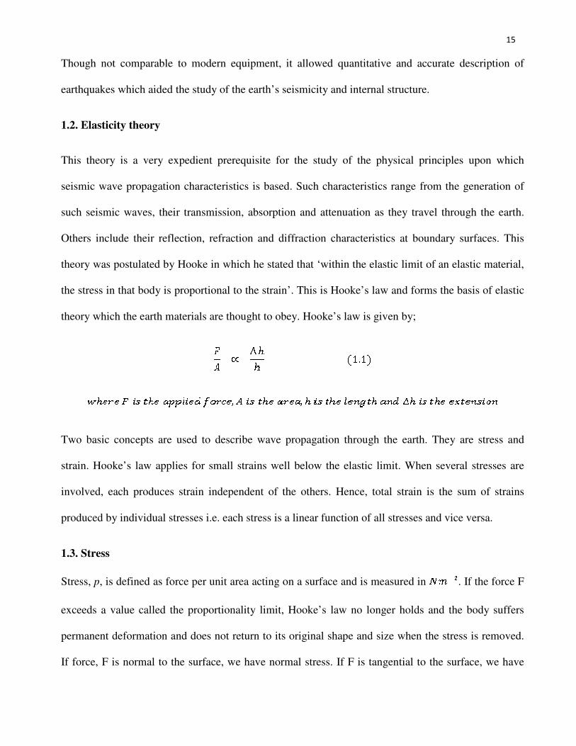
theory which the earth materials are thought to obey. Hooke’s law is given by;

Two basic concepts are used to describe wave propagation through the earth. They are stress and

strain. Hooke’s law applies for small strains well below the elastic limit. When several stresses are

involved, each produces strain independent of the others. Hence, total strain is the sum of strains

produced by individual stresses i.e. each stress is a linear function of all stresses and vice versa.

1.3. Stress

Stress, p, is defined as force per unit area acting on a surface and is measured in . If the force F

exceeds a value called the proportionality limit, Hooke’s law no longer holds and the body suffers

permanent deformation and does not return to its original shape and size when the stress is removed.

If force, F is normal to the surface, we have normal stress. If F is tangential to the surface, we have

16

shearing stress. If F is neither parallel nor perpendicular to element of surface, it can be resolved into

normal or shearing stresses.

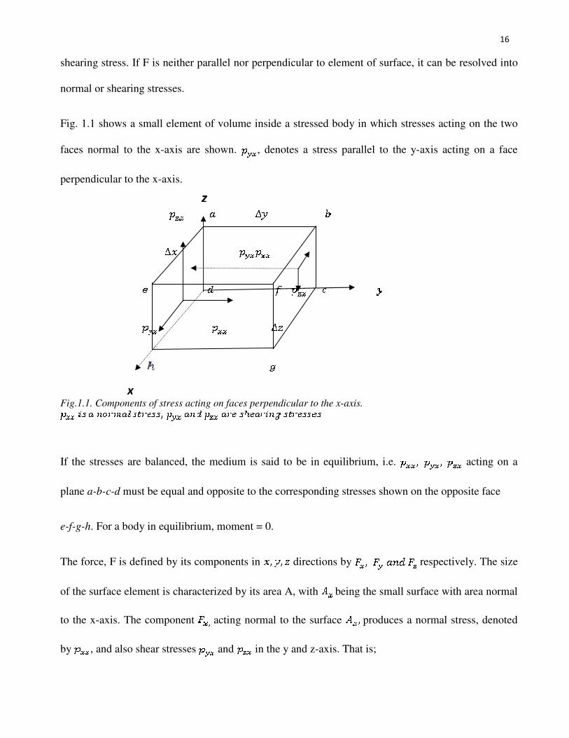
Fig. 1.1 shows a small element of volume inside a stressed body in which stresses acting on the two

faces normal to the x-axis are shown. , denotes a stress parallel to the y-axis acting on a face

perpendicular to the x-axis.

Fig.1.1. Components of stress acting on faces perpendicular to the x-axis.

If the stresses are balanced, the medium is said to be in equilibrium, i.e. acting on a

plane a-b-c-d must be equal and opposite to the corresponding stresses shown on the opposite face

e-f-g-h. For a body in equilibrium, moment = 0.

The force, F is defined by its components in directions by respectively. The size

of the surface element is characterized by its area A, with being the small surface with area normal

to the x-axis. The component acting normal to the surface produces a normal stress, denoted

by , and also shear stresses and in the y and z-axis. That is;

x

z

17

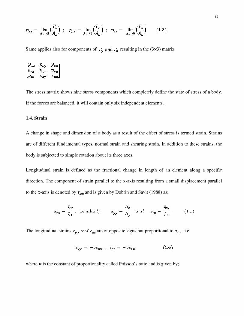
Same applies also for components of resulting in the (3×3) matrix

The stress matrix shows nine stress components which completely define the state of stress of a body.

If the forces are balanced, it will contain only six independent elements.

1.4. Strain

A change in shape and dimension of a body as a result of the effect of stress is termed strain. Strains

are of different fundamental types, normal strain and shearing strain. In addition to these strains, the

body is subjected to simple rotation about its three axes.

Longitudinal strain is defined as the fractional change in length of an element along a specific

direction. The component of strain parallel to the x-axis resulting from a small displacement parallel

to the x-axis is denoted by and is given by Dobrin and Savit (1988) as;

The longitudinal strains are of opposite signs but proportional to . i.e

where is the constant of proportionality called Poisson’s ratio and is given by;

18

Dilatation, which is defined as the fractional change in volume per unit volume of an element in the

limit when its surface area decreases to zero and is given (Lowrie, 2007) by;

Shear strain is a products of the shear components of stress ( ) due to changes in the

angular relationship between parts of a body. When for instance, a square is sheared parallel to the x-

axis, the side parallel to the y-axis rotates through an angle . When it is sheared parallel to the y-

axis, the side parallel to the x-axis rotates through an angle .

The shear strain in the x-y plane is half the total angular distortion (Lowrie, 2007). i.e.

It could be illustrated in a symmetric 3×3 strain matrix as

19

The deformation of a body gives rise to a relationship between stress and strain. The ratio of such

relationship defines the elastic modulus of that body. The unit for elastic moduli is (Newton

per meter squared). Elastic moduli is defined for three types of deformation;

i. Young’s modulus, E: This results from deformation due to extension. i.e.

,

where E is Young’s modulus and is the constant of proportionality.

ii. Shear or rigidity modulus, : This results from shear deformation. i.e.

,

where constant of proportionality is shear modulus .

In terms of Young’s modulus and Poisson’s ratio, is given by

iii. Bulk Modulus, K : This is the ratio of hydrostatic pressure to the dilatation. That is

where P is the hydrostatic pressure, K is Bulk modulus and is the dilatation.

In terms of Young’s modulus and Poisson’s ratio, is given by Telford (1990) as,

(1.8)

1.5. Seismic wave equation

To derive the wave equation for both P and S waves, we consider the stress-strain diagram (fig. 1.1),

from which we obtain the stresses on the front face e-f-g-h, as,

(1.9)

Because these stresses are opposite to those acting on the rear face a – b – c - d, some stresses balance

and cancel out. Unbalanced stresses are given as;

20

Hence, the net forces acting per unit volume in the x, y, z directions have values;

Other faces hold similar expressions. Therefore, we derive total force per unit volume in the x-

direction as

We apply Newton’s second law to the total force per unit volume in the x-direction to set;

(1.10)

where U is displacement in x-direction and is the body density.

Equation 1.10 relates the displacement to the stresses.

But by Hooke’s law,

Likewise, .

We substitute these expressions in equation (1.11) also noting that

, (1.12)

where is called dilatation and is defined as the fractional change in volume per unit volume of an

element in the limit when its surface area decreases to zero.

We therefore obtain the expression;

21

Similarly, the corresponding expressions for and are

By multiplying (1.13 a) by i, (1.13 b) by j and (1.13 c) by k, we obtain

By defining displacement as becomes

Equation (1.15) is the equation of wave propagation in a homogeneous isotropic elastic solid. It is an

approximate expression which neglects body forces such as gravity and velocity gradient terms and

assumes a linear isotropic earth model.

If we take the divergence of both sides of (1.15), we obtain

But,

Equation (1.16) then becomes,

=

Equation (1.17) is the P-wave equation in which dilatation propagates with a velocity,

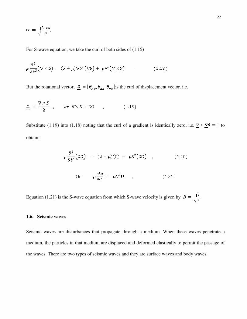
22

.

For S-wave equation, we take the curl of both sides of (1.15)

But the rotational vector, = is the curl of displacement vector. i.e.

Substitute (1.19) into (1.18) noting that the curl of a gradient is identically zero, i.e. to

obtain;

Or

Equation (1.21) is the S-wave equation from which S-wave velocity is given by .

1.6. Seismic waves

Seismic waves are disturbances that propagate through a medium. When these waves penetrate a

medium, the particles in that medium are displaced and deformed elastically to permit the passage of

the waves. There are two types of seismic waves and they are surface waves and body waves.

23

1.6.1. Body waves

These are waves or energy that propagates through the body of the medium. They gradually transform

from spherical waves to plane waves as the distance from its source increases due to the reduction in

curvature of its wave front. Body waves are of two types, longitudinal and transverse waves.

Longitudinal or compressional waves are waves that pass through a medium as a series of rare-

factions (dilatations) and compressions.

Transverse or shear waves are concerned with the vibrations along the y and z directions which are

parallel to the wavefront and transverse to the direction of propagation in the x-direction.

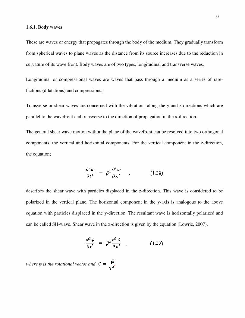
The general shear wave motion within the plane of the wavefront can be resolved into two orthogonal

components, the vertical and horizontal components. For the vertical component in the z-direction,

the equation;

describes the shear wave with particles displaced in the z-direction. This wave is considered to be

polarized in the vertical plane. The horizontal component in the y-axis is analogous to the above

equation with particles displaced in the y-direction. The resultant wave is horizontally polarized and

can be called SH-wave. Shear wave in the x-direction is given by the equation (Lowrie, 2007),

where ψ is the rotational vector and .

24

Longitudinal waves are the fastest of all seismic waves and so arrive first at a detector (seismometer)

when an earthquake occurs. The first arrivals are called primary waves (P-waves). P-waves travel

through solid, liquid and gas because they are compressible. Transverse waves on the other hand are

much slower and so constitute later arrivals at recording stations. These waves are called secondary

waves (S-waves). They penetrate solids but can’t transmit through liquids and gases.

1.6.2. Surface waves

These are disturbances propagating close to a free surface of a medium. Surface waves are classified

into several types, the most common types are Love waves and Rayleigh waves.

Love wave are waves that can propagate only in a velocity layered medium. The particle motion is

horizontal and perpendicular to the direction of propagation, with its amplitude decreasing with depth.

For a two-layer medium with S-wave velocities and , with Love waves of short wavelengths

closer to the slower velocity and long wavelengths travelling at speed closer to the faster velocity,

. Love waves are dispersive (Lowrie, 2007).

At the surface of homogenous and isotropic half space, the particles in Rayleigh waves are polarized

to vibrate in the vertical plane containing the direction of wave motion. The resulting particle motion

is a combination of the P and SV-vibrations. Rayleigh waves are non-dispersive. Raleigh waves

(often called ground roll) are a main source of signal generated noise on seismic reflection records.

1.7. Seismic wave propagation

Propagation of waves through a medium is as a result of the periodic elastic displacements of the

particles in that medium and its progress is determined by the advancement of the wavefront. Two

principles can be used to handle this. These principles are Huygen’s principle and Fermat’s principle.

25

1.7.1. Huygen’s Principle:

This principle as proposed by a Dutch mathematician/physicist, Christiaan Huygens in 1678 describes

the behavior of wavefronts. It is based on simple geometrical construction. It states that “all points on

a wavefront can be regarded as source points for the production of new spherical waves. The new

wavefront is the tangential surface or envelope of the secondary wavelets”. This method permits the

calculation of the future position of a wavefront if the present position is known. This principle is

applied in reflection and refraction, mainly at their boundaries.

1.7.2. Fermat’s Principle:

Formulated by a French mathematician, Pierre de Fermat, this principle states that of the many

possible paths between two points, the seismic ray will follow the path that gives the shortest travel-

time between the points. This principle describes the geometry of the ray paths at an interface.

1.8. Wave attenuation

This is the decrease of amplitude of a wave with increasing distance from the source. This reduction

is due to either the geometry of the propagation of the wave or the anelastic property of the medium

through which the wave travel. Amplitude attenuation is more rapid in body waves than in surface

waves. They have a corresponding attenuation of respectively.

Absorption of energy due to imperfect elastic property of the medium causes attenuation. This is as a

result of energy loss amongst rock particles and can also be called anelastic damping. Damping of

waves is described by a parameter called quality factor which is defined as the fractional loss of

energy per cycle. Damped amplitude of a seismic wave at distance r from its source is given (Lowrie,

2007) by;

26

where D is the distance within which the amplitude falls to of its original value.

Its follows from equation (1.24) that absorption co-efficient is inversely proportional to the

wavelength and is dependent on the frequency of the signal.

1.9. Seismic velocity

Velocity plays an important role in data interpretation. The knowledge of seismic velocity values is

very necessary in the determination of depth and dip of reflectors and refractors and in the general

assessment of the nature of the rocks and interstitial fluids in the sub-surface. Velocity is obtained

from measurements taken in the field, well logging or from samples in the laboratory.

There are different types of velocity. These include average velocity, root mean square velocity,

interval velocity, phase velocity, stacking velocity, instantaneous velocity and apparent velocity

Average velocity is defined as the distance travelled divided by the time taken to traverse path. Root

mean square velocity refers to the velocity of a specific ray path as it travels through layers. Interval

velocity on the other hand is the average velocity over some interval of the travel path. Phase velocity

refers to the velocity of perpendicular distances between phases of a wavefront. Stacking velocity is

the velocity value determined by velocity analysis usually made by finding the best fitting hyperbola

to data that are not perfectly hyperbolic. It is used to correct the quasi-hyperbolic primary reflection

event to time alignment with zero offset. Instantaneous velocity is the velocity with which a

wavefront passes through a point measured in the direction of travel. Apparent velocity refers to the

apparent speed of a given phase in a particular direction usually, spread direction on the surface.

27

1.10. Factors that affect seismic velocity

Due to the non-homogenous nature of the earth, seismic velocity varies from location to location and

an understanding of these factors helps us foresee the kinds of velocity variations to expect in such

areas. Such factors include effect of lithology (that is rock type), effect of density (where velocity is

higher in more dense rocks), porosity of rocks, depth of burial (in which case the greater the depth of

burial, the more the pressure and consequently, higher velocity). The age of the rock type is another

factor. Others are effect of interstitial fluid where more pore fluid depicts lower velocity, temperature,

frequency etc.

1.11. Purpose of study

The purpose of this study is to intensively review the different approaches applied to seismic

reflection survey and the results obtained during several operations as carried out in different parts of

the world. The study and comparison of these seismic reflection operations and the results obtained is

aimed at suggesting a more appropriate procedure in seismic data collection, processing and

interpretation, for yielding more robust results.

28

CHAPTER TWO

SEISMIC DATA ACQUISITION AND PROCESSING

2.1. Introduction

Over the decade, seismology has become the key tool to exploration and developmental successes.

With advancements in computer technology, data processing has increasingly acquired a competitive

edge and resulted in the production of clearer and more detailed seismic sections. There is no specific

or generally accepted mode of processing but the choice of a processing method depends on the

information hoped to be obtained or simply the choice of the analyst. The choice of equipment also

determines processing sequence. We should also bear in mind that there are also a variety of

objectives for which a data can be used. Data processing to a certain degree can be adjusted to meet

specific requirement. Seismic data processing is characterized by a sequence of steps where for each

of these steps, there exists a multitude of different approaches.

2.2. Seismic data acquisition

Seismic data acquisition requires a controlled source of energy or signal, usually an explosion or

vibration sent into the ground at a known time and location. By taking note of the time it takes the

signal to be reflected back from the boundaries between rocks to a receiver on the earth’s surface

(usually a geophone for land use and a hydrophone for marine), the depths and features of the sub-

surface interfaces can be estimated after some processing and analyses.

Seismic data could be acquired on land (land survey) or over an aquatic environment (marine

survey). Both methods employ the same principle of sending signals into the ground and recording

the two-way travel time even though the equipment used differs. Energy sources for land survey

29

include explosives, impact sources (weight drop), vibrators and even hammer for shallow small-

scale exploration while for marine surveys, airgun, watergun, marine vibrators, aquapulse,

maxipulse, flexotir etc. are employed.

Several field procedures are in use, each being distinguished by the different layout of the

geophones relative to the shot-point. Continuous profiling is usually the routine in which the shot-

point and geophones are moved a predetermined distance after each shot is taken. Continuous

profiling could be conventional i.e. when a reflecting point is sampled once, or redundant, when it is

sampled more than once. Continuous profiling aims at reducing seismic noise. Split spreading is the

most common form of convectional coverage in which the geophones are symmetrically spread on

either side of the shot-point while the common mid-point (CMP) method is an illustration of the

redundant coverage in which shots are fired at different points and each shot has a sub-surface

coverage such that by repeatedly moving the shot-point and geophone arrays, each reflecting point

on the interface is sampled severally

As the geophones/hydrophones detect the arrival of seismic waves, the signals are converted to a

digital form in the present day, unlike in the early systems which recorded analogue signals directly to

magnetic tapes or photographic films. The recorded signals are then displayed by a computer as

seismograms for processing and analysis.

2.3. Seismic data processing

The main goal of seismic processing is to construct high quality reflectivity images of the investigated

sub-surface. Bearing in mind the inhomogenity of the earth, several factors such as environmental and

demographic restrictions can have significant impact on data quality. Other factors such as field

geometry and conditions of recording could also pull strings. Having knowledge of these restricting

factors and the need to have a clearer picture of the sub-surface to compensate for the whole effort

30

and finance put in is necessary. Therefore, obtained data undergo several stages of processing, all

primarily aimed at increasing the signal to noise ratio, thus, producing genuine reflections which

could be interpreted.

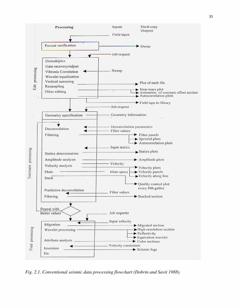
Seismic data processing comprises of three main stages; the pre-processing stage, the main processing

stage and the final processing stage as illustrated in fig 2.1.

2.4. Pre-processing

Pre-processing, as can be coined from its name, are processing operations that are carried out on the

field data before the main processing. Such operations include demultiplexing (reformatting), muting,

gain application, filtering and identing. Let us consider them briefly.

2.4.1. Demultiplexing

Field data are recorded in multiplexed form. A multiplexed data is a continuous stream of seismic

samples for the whole seismic record. i.e. in rows of samples at the same time at consecutive

channels. A digital sample is recorded for each seismic trace at a pre-selected sampling rate (2ms or

4ms) in rows of samples at several channels, consecutively. Demultiplexing sorts these data into

columns of samples, i.e. all the time samples in one channel, followed by those in the next channel

and so on.

31

Fig. 2.1. Conventional seismic data processing flowchart (Dobrin and Savit 1988).

32

It can be said that demultiplexing is the separating of all the samples to produce a time sequence for

each geophone. Mathematically, it could be seen as transposing a big matrix such that the column of

the resulting matrix can be read as seismic traces recorded at different offsets with a common shot-

point (Hatton et al, 1986).

Multiplexed data are time sequential while demultiplexed data are trace sequential.

2.4.2. Trace editing and muting

This is a manual cleaning up process of the data. Dead traces, noisy traces (ground rolls, direct

arrivals), mono-frequency signals with transient glitches and less relevant events are deleted and

polarity of reverse traces switched. Frequency distorted zones are also muted to avoid them

suppressing shallow events.

2.4.3. Gain recovery

This function is applied to data to correct for the amplitude effect of spherical wavefront divergence.

This involves the application of a geometric spreading function which depends on travel-time and an

average primary velocity function which is associated with primary reflections in the survey area. It

will also require an exponential gain function to compensate for attenuation losses.

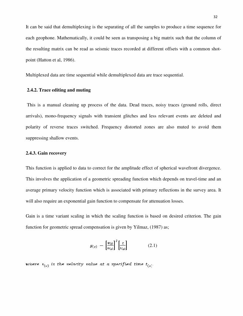
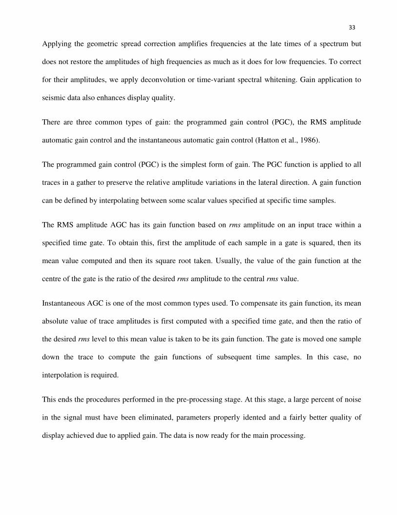
Gain is a time variant scaling in which the scaling function is based on desired criterion. The gain

function for geometric spread compensation is given by Yilmaz, (1987) as;

(2.1)

33

Applying the geometric spread correction amplifies frequencies at the late times of a spectrum but

does not restore the amplitudes of high frequencies as much as it does for low frequencies. To correct

for their amplitudes, we apply deconvolution or time-variant spectral whitening. Gain application to

seismic data also enhances display quality.

There are three common types of gain: the programmed gain control (PGC), the RMS amplitude

automatic gain control and the instantaneous automatic gain control (Hatton et al., 1986).

The programmed gain control (PGC) is the simplest form of gain. The PGC function is applied to all

traces in a gather to preserve the relative amplitude variations in the lateral direction. A gain function

can be defined by interpolating between some scalar values specified at specific time samples.

The RMS amplitude AGC has its gain function based on rms amplitude on an input trace within a

specified time gate. To obtain this, first the amplitude of each sample in a gate is squared, then its

mean value computed and then its square root taken. Usually, the value of the gain function at the

centre of the gate is the ratio of the desired rms amplitude to the central rms value.

Instantaneous AGC is one of the most common types used. To compensate its gain function, its mean

absolute value of trace amplitudes is first computed with a specified time gate, and then the ratio of

the desired rms level to this mean value is taken to be its gain function. The gate is moved one sample

down the trace to compute the gain functions of subsequent time samples. In this case, no

interpolation is required.

This ends the procedures performed in the pre-processing stage. At this stage, a large percent of noise

in the signal must have been eliminated, parameters properly idented and a fairly better quality of

display achieved due to applied gain. The data is now ready for the main processing.

34

2.5. Main processing

There are three basic stages in seismic data processing. These stages are deconvolution, stacking and

migration. Each of these satisfies the goal of data processing which is improvement of the temporal

resolution of seismic data (deconvolution), enhanced signal to noise ratio (stacking) and improvement

of lateral resolution (migration).

Other processes involved in the main processing stage include normal move-out (NMO) correction,

elevation correction, dip move-out (DMO) correction and frequency filtering.

NMO correction compensates for differences in travel times due to differences in source-receiver

offset so that all traces having the same common mid-point (CMP) would appear to have zero offsets

and combined as one. This combination of traces having the same CMP is referred to as stacking.

CMPs are sorted out using a binning grid superimposed over the survey area. The grid is usually

oriented along the actual shot and geophone lines or for marine prospect, along the shooting direction.

The dimensions of the bins are usually based on the shot spacing and geophone spacing. A number of

traces or CMP will fall within each grid cell or bin. These traces are assumed to be imaging the same

general area of the sub-surface.

After applying NMO and static corrections, there is need to perform the dip move-out (DMO)

correction to correct for travel time differences due to dipping reflectors. The traces are then stacked

within each bin to produce a single trace usually at the bin centroid. After stacking, other multi-trace

processes such as migration are possible.

Some factors can just not be left out. In the processing stage, about the most important element is the

velocity information. Without this information, NMO, DMO and static corrections would not be

feasible. CMP stacking, migration and time-depth conversion will also not be possible. This makes it

very expedient.

35

Velocity information also helps in rock identification. Before the computer era, velocity

determination used to be analytic but these days, velocity can be determined directly from reflection

data, well logs, sonic logs etc.

Filtering is another sequence in the processing stage. As the name implies, it simply means

eliminating unwanted data. But in this case, it is usually data outside a particular range. There are

several types of filters and they will be discussed in a few pages.

2.5.1. Deconvolution

Deconvolution aims at generating a smoothly tampered wavelet with a wide spectrum. It improves

temporal resolution by compressing effective source wavelet contained in the seismic trace to a spike

of zero-lag. This is called spiking deconvolution. Since this broadens the spectrum of seismic data,

traces tend to contain much more high frequency energy after deconvolution. To have a better

understanding of the deconvolution process, let us take a brief look at convolution and its model.

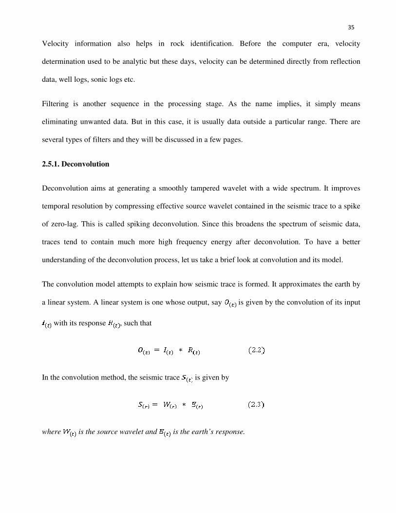
The convolution model attempts to explain how seismic trace is formed. It approximates the earth by

a linear system. A linear system is one whose output, say is given by the convolution of its input

with its response , such that

In the convolution method, the seismic trace is given by

where is the source wavelet and is the earth’s response.

36

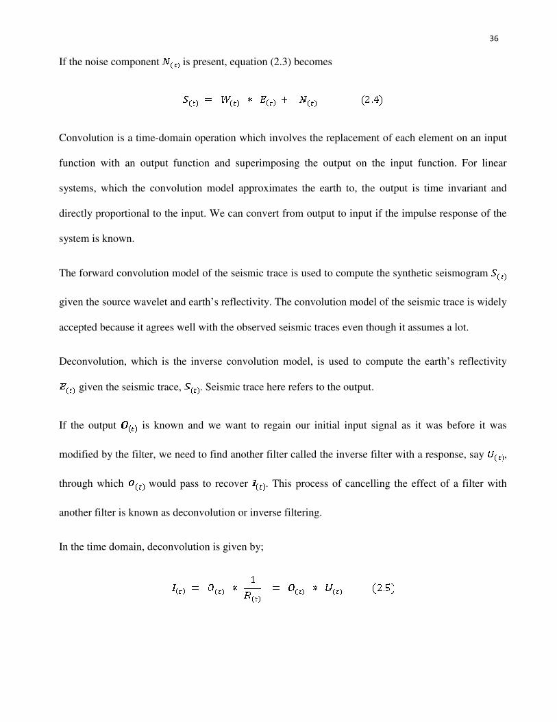
If the noise component is present, equation (2.3) becomes

Convolution is a time-domain operation which involves the replacement of each element on an input

function with an output function and superimposing the output on the input function. For linear

systems, which the convolution model approximates the earth to, the output is time invariant and

directly proportional to the input. We can convert from output to input if the impulse response of the

system is known.

The forward convolution model of the seismic trace is used to compute the synthetic seismogram

given the source wavelet and earth’s reflectivity. The convolution model of the seismic trace is widely

accepted because it agrees well with the observed seismic traces even though it assumes a lot.

Deconvolution, which is the inverse convolution model, is used to compute the earth’s reflectivity

given the seismic trace, . Seismic trace here refers to the output.

If the output is known and we want to regain our initial input signal as it was before it was

modified by the filter, we need to find another filter called the inverse filter with a response, say ,

through which would pass to recover . This process of cancelling the effect of a filter with

another filter is known as deconvolution or inverse filtering.

In the time domain, deconvolution is given by;

37

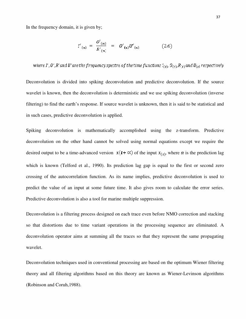
In the frequency domain, it is given by;

Deconvolution is divided into spiking deconvolution and predictive deconvolution. If the source

wavelet is known, then the deconvolution is deterministic and we use spiking deconvolution (inverse

filtering) to find the earth’s response. If source wavelet is unknown, then it is said to be statistical and

in such cases, predictive deconvolution is applied.

Spiking deconvolution is mathematically accomplished using the z-transform. Predictive

deconvolution on the other hand cannot be solved using normal equations except we require the

desired output to be a time-advanced version of the input , where is the prediction lag

which is known (Telford et al., 1990). Its prediction lag gap is equal to the first or second zero

crossing of the autocorrelation function. As its name implies, predictive deconvolution is used to

predict the value of an input at some future time. It also gives room to calculate the error series.

Predictive deconvolution is also a tool for marine multiple suppression.

Deconvolution is a filtering process designed on each trace even before NMO correction and stacking

so that distortions due to time variant operations in the processing sequence are eliminated. A

deconvolution operator aims at summing all the traces so that they represent the same propagating

wavelet.

Deconvolution techniques used in conventional processing are based on the optimum Wiener filtering

theory and all filtering algorithms based on this theory are known as Wiener-Levinson algorithms

(Robinson and Coruh,1988).

38

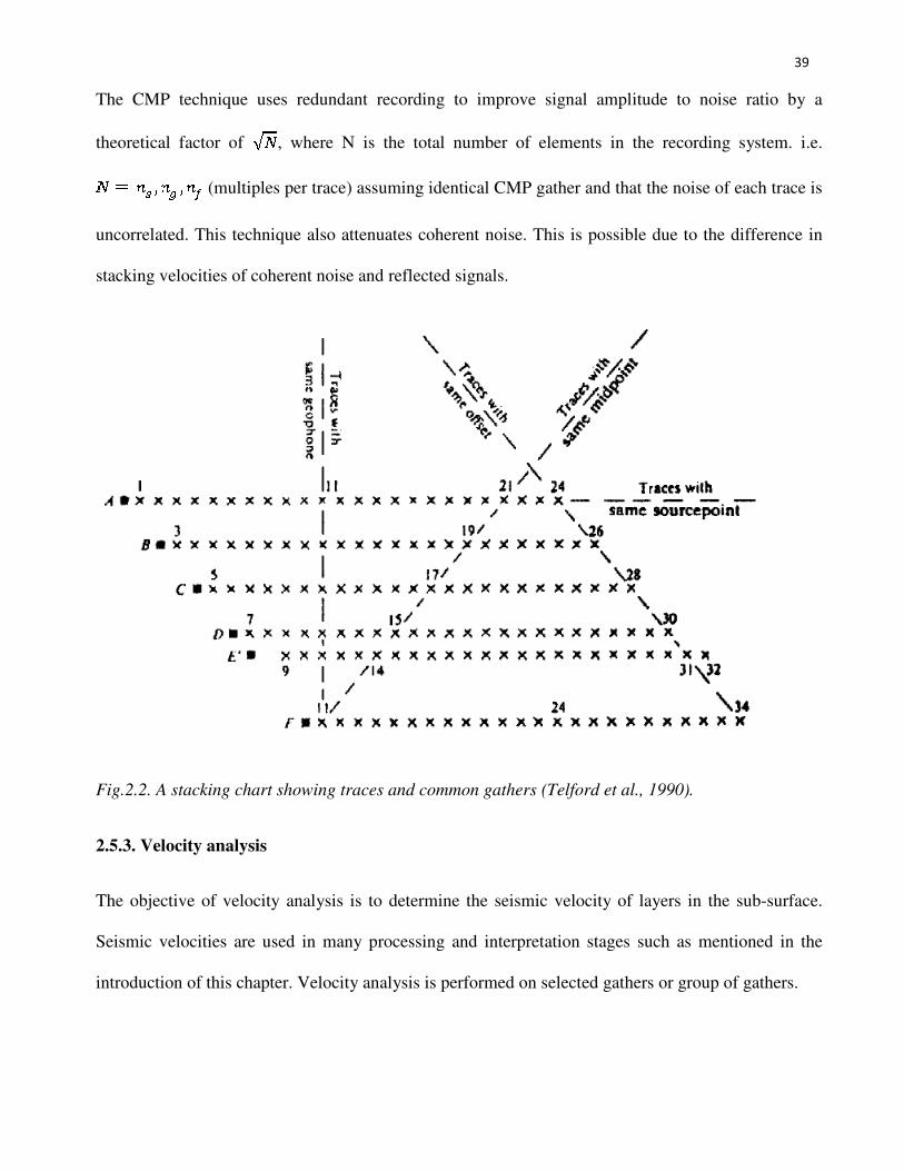
2.5.2. CMP sorting

This is the transformation of data from shot-receiver to mid-point-offset coordinates. It requires

information about the field geometry. Conventional seismic data processing is done using midpoint-

offset coordinates and this is achieved by first sorting the data into CMP gathers. Traces with the

same mid-points are grouped together to form a CMP gather. Fig. 2.2 shows a stacking chart which

will make our understanding of these gathers clearer.

Stacking charts are useful when setting up the geometry of a line for pre-processing and makes

identification of missing traces easy to find.

Due to the large number of traces involved in CMP acquisition, a stacking chart is used to keep track

of values. A Stacking chart could either be surface, which has geophone location g, as one coordinate

or source location s, as another or sub-surface, which has the trace plotted at (Telford

et al., 1990).

Stacking charts are useful in making static and NMO corrections and ensuring proper trace tracking.

Displays of the data in different directions are called gathers or domains. We have the common

source gather, common geophone gather, common mid-point gather and common offset gather. All

these prove useful in the study of noise such as multiples, ghosts, converted waves etc. For horizontal

interfaces, a source placed at the centre of a geophone spread will give a symmetrical curve about the

source point. If however the reflector has a uniform dip, the path of reflected ray on the down-dip side

of the shot-point will be longer than those on the up-dip side and this has corresponding effect on the

travel times. If reflected records are not corrected for layer dip, an error results in plotting the position

of dipping beds.

39

The CMP technique uses redundant recording to improve signal amplitude to noise ratio by a

theoretical factor of , where N is the total number of elements in the recording system. i.e.

(multiples per trace) assuming identical CMP gather and that the noise of each trace is

uncorrelated. This technique also attenuates coherent noise. This is possible due to the difference in

stacking velocities of coherent noise and reflected signals.

Fig.2.2. A stacking chart showing traces and common gathers (Telford et al., 1990).

2.5.3. Velocity analysis

The objective of velocity analysis is to determine the seismic velocity of layers in the sub-surface.

Seismic velocities are used in many processing and interpretation stages such as mentioned in the

introduction of this chapter. Velocity analysis is performed on selected gathers or group of gathers.

40

The output of one type of velocity analysis is a table of numbers as a function of velocity versus two-

way zero offset time (velocity spectrum). These numbers represent some measure of coherency along

the hyperbolic trajectories governed by velocity, offset and travel-time. Velocity time pairs are

selected from velocity spectrum based on maximum coherency peaks. These velocity functions are

then spatially interpolated between the analysis points across the entire profile. When velocity picks

become inaccurate due to complex structures, the data could be stacked with a range of constant

velocities which are then used to pick the velocities.

NMO and stacking velocities can be derived from T-X data. The T-X curve of a single constant

velocity horizontal layer is a perfect hyperbola given by

where is the two-way travel time at offset and is the two-way travel time at zero offset, is

the layer velocity. (Hatton et al., 1986).

The rms velocity can be defined in terms of the true T-X curve as the square root of the reciprocal of

the coefficient of the term in the series approximation of the exact curve for multiple

layers. It can be shown that is equal to the square root of the reciprocal of the slope of the

tangent to the exact curve at x = 0, that is;

where c is the wave velocity

41

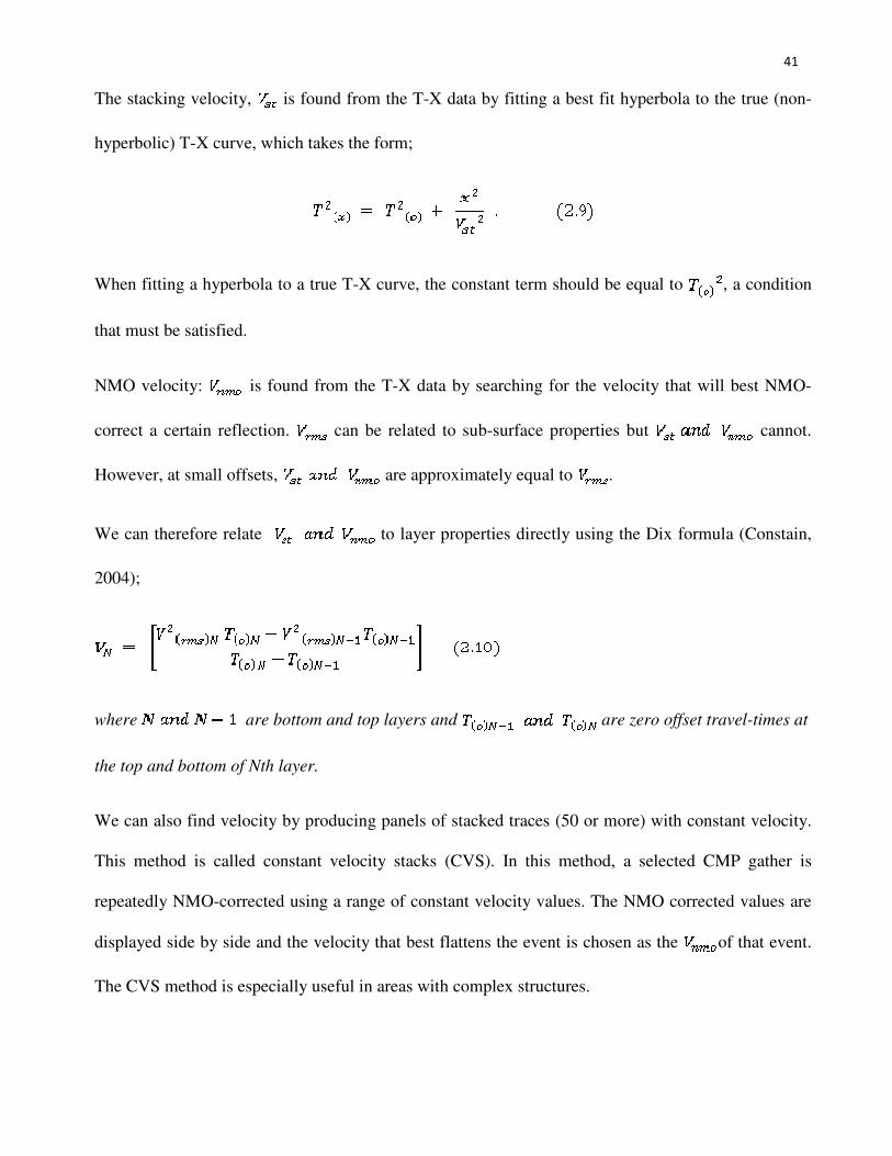
The stacking velocity, is found from the T-X data by fitting a best fit hyperbola to the true (non-

hyperbolic) T-X curve, which takes the form;

When fitting a hyperbola to a true T-X curve, the constant term should be equal to , a condition

that must be satisfied.

NMO velocity: is found from the T-X data by searching for the velocity that will best NMO-

correct a certain reflection. can be related to sub-surface properties but cannot.

However, at small offsets, are approximately equal to .

We can therefore relate to layer properties directly using the Dix formula (Constain,

2004);

where are bottom and top layers and are zero offset travel-times at

the top and bottom of Nth layer.

We can also find velocity by producing panels of stacked traces (50 or more) with constant velocity.

This method is called constant velocity stacks (CVS). In this method, a selected CMP gather is

repeatedly NMO-corrected using a range of constant velocity values. The NMO corrected values are

displayed side by side and the velocity that best flattens the event is chosen as the of that event.

The CVS method is especially useful in areas with complex structures.

42

The velocity spectrum attempts to find the stacking velocity to each reflector. It maps the T-X data of

a single CMP gather onto the velocity-spectrum plane where the vertical axis is the and the

horizontal axis is . The velocity spectrum method is more suitable for noise contaminated datasets.

Spread length, stacking fold, S/N ratio, time gate length etc. are some factors that limit the accuracy

and resolution of this method.

2.5.4. NMO correction

NMO is a non-linear stretching of the seismic time axis. To remove travel-time components due to

source-receiver offset, NMO correction is applied. NMO correction prepares the data for stacking and

finds the NMO velocity to the reflector.

After NMO corrections, the events are noticed to be virtually flattened across the offset range. The

resultant effect of this is the stretching of traces in a time-varying manner consequently, shifting the

frequency component towards the left end of its spectrum. If a high velocity is used for NMO

correction, the event would be under-corrected or over-corrected if a lower velocity is used (fig.2.3).

The right velocity will align the event horizontally at .

Because velocity increases with depth, the NMO correction applied for a later will be smaller than

that applied to an earlier . Therefore, the two events with a time separation equal to before

NMO correction will have a separation of after NMO correction. This is called NMO

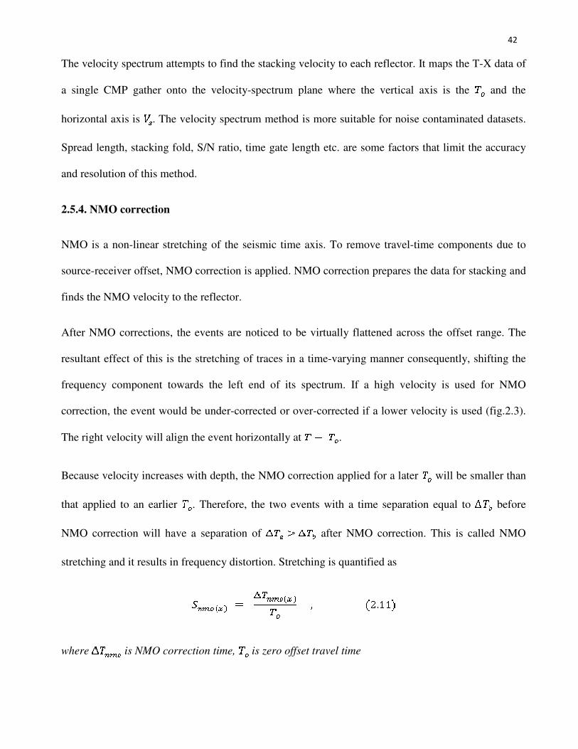
stretching and it results in frequency distortion. Stretching is quantified as

where is NMO correction time, is zero offset travel time

43

It is only but wise to remove the stretching before stacking. This is done by muting the considerably

stretched zones from the gather.

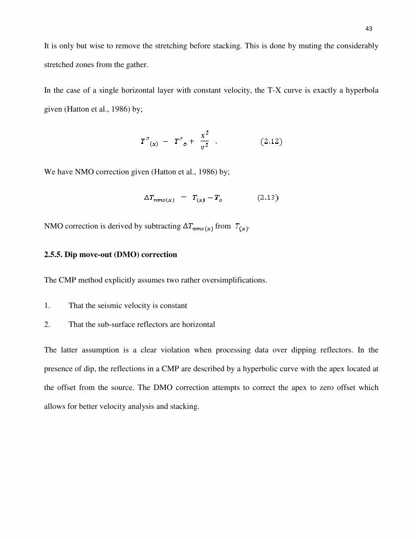
In the case of a single horizontal layer with constant velocity, the T-X curve is exactly a hyperbola

given (Hatton et al., 1986) by;

We have NMO correction given (Hatton et al., 1986) by;

NMO correction is derived by subtracting from .

2.5.5. Dip move-out (DMO) correction

The CMP method explicitly assumes two rather oversimplifications.

1. That the seismic velocity is constant

2. That the sub-surface reflectors are horizontal

The latter assumption is a clear violation when processing data over dipping reflectors. In the

presence of dip, the reflections in a CMP are described by a hyperbolic curve with the apex located at

the offset from the source. The DMO correction attempts to correct the apex to zero offset which

allows for better velocity analysis and stacking.

44

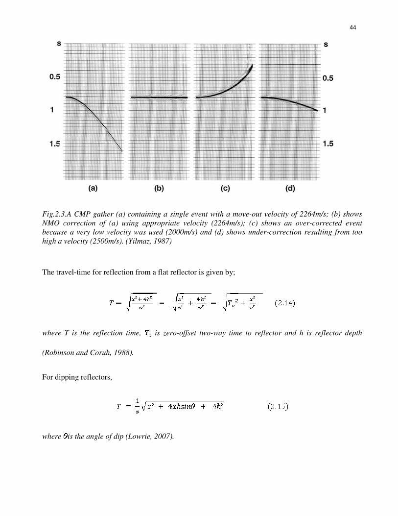
Fig.2.3.A CMP gather (a) containing a single event with a move-out velocity of 2264m/s; (b) shows

NMO correction of (a) using appropriate velocity (2264m/s); (c) shows an over-corrected event

because a very low velocity was used (2000m/s) and (d) shows under-correction resulting from too

high a velocity (2500m/s). (Yilmaz, 1987)

The travel-time for reflection from a flat reflector is given by;

where T is the reflection time, is zero-offset two-way time to reflector and h is reflector depth

(Robinson and Coruh, 1988).

For dipping reflectors,

where is the angle of dip (Lowrie, 2007).

45

Equation 2.15 can be expressed in a hyperbolic form as;

with axis of symmetry given by .

The benefits of DMO correction include noise filtering through dip filtering, minimized reflection

point scatter, improved velocity analysis, improved ties with crossing lines etc.

2.5.6. Statics corrections

CMP gathers don’t always conform to a perfect hyperbolic trajectory. A cause of this could be as a

result of near surface irregularities. Lateral velocity variations could cause a reflection event to switch

from long offset traces to short offset traces (negative move-out) as a result of complex overburden.

Static correction is targeted towards compensating for elevation differences such that all traces are

corrected to a datum level by removing the calculated travel times from the source to the datum and

from the receiver to the datum. Fig. 2.4 illustrates this concept.

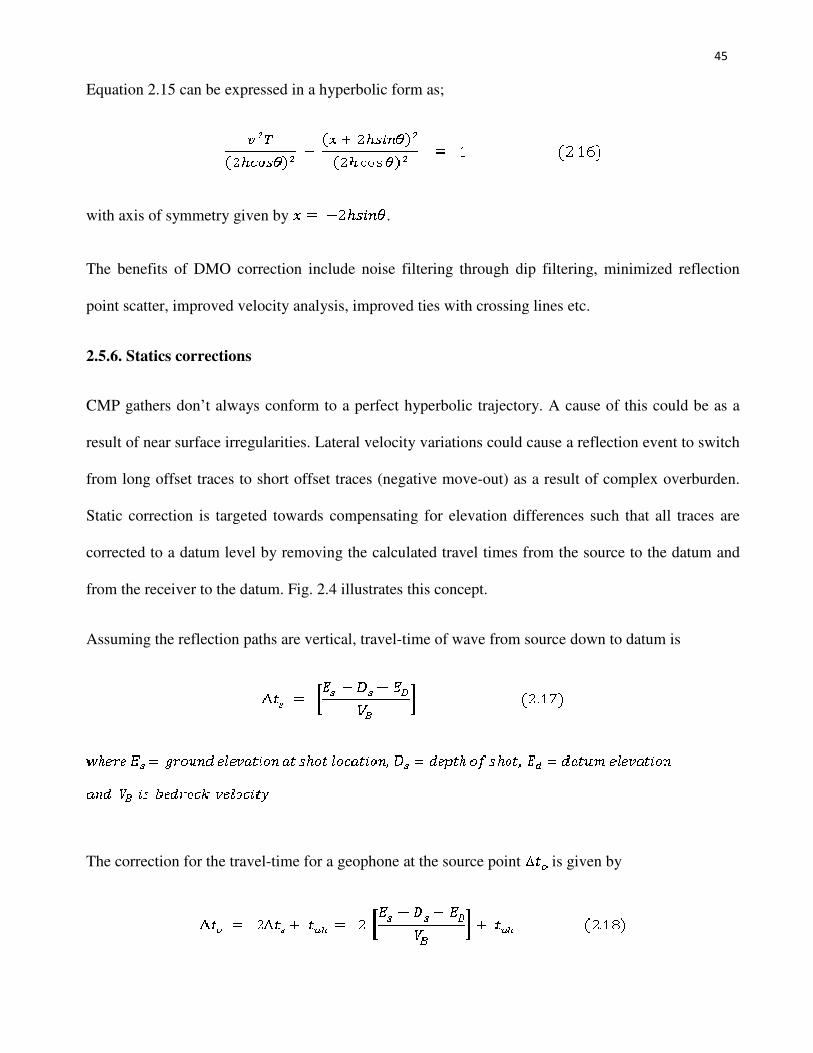
Assuming the reflection paths are vertical, travel-time of wave from source down to datum is

The correction for the travel-time for a geophone at the source point is given by

46

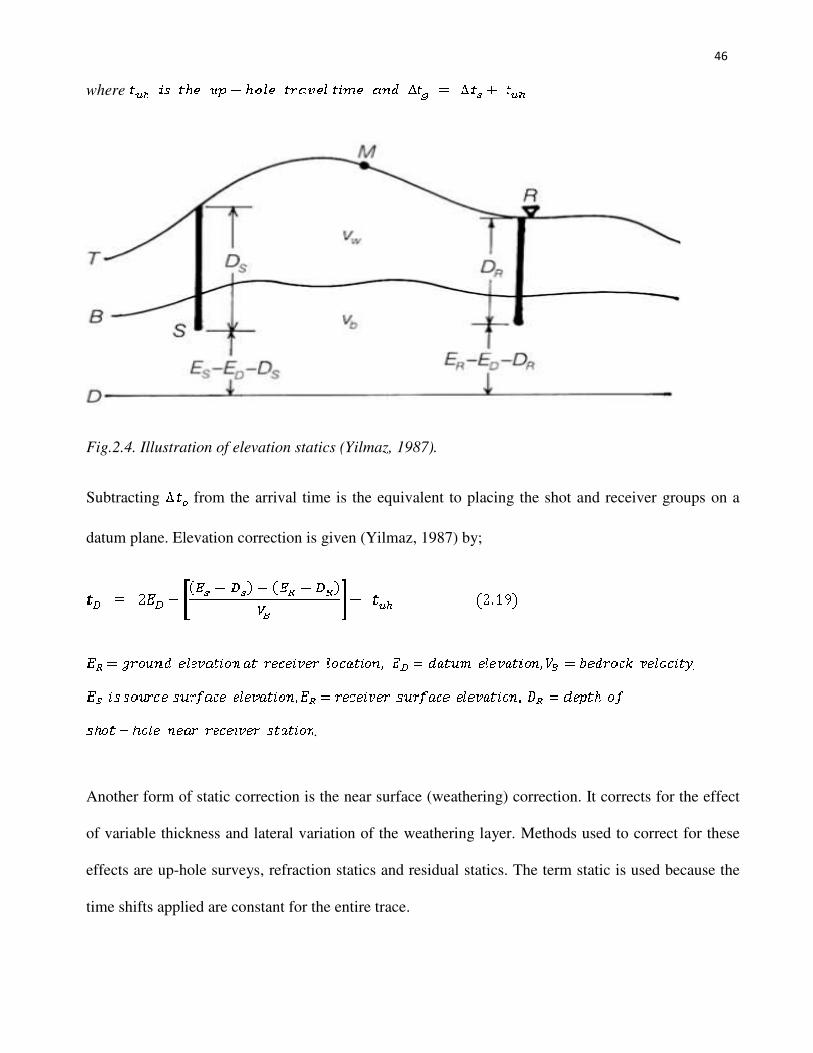
where

Fig.2.4. Illustration of elevation statics (Yilmaz, 1987).

Subtracting from the arrival time is the equivalent to placing the shot and receiver groups on a

datum plane. Elevation correction is given (Yilmaz, 1987) by;

.

Another form of static correction is the near surface (weathering) correction. It corrects for the effect

of variable thickness and lateral variation of the weathering layer. Methods used to correct for these

effects are up-hole surveys, refraction statics and residual statics. The term static is used because the

time shifts applied are constant for the entire trace.

47

2.5.7. Residual statics correction (RSC)

Of course, little random errors in static alignment on traces remain after static corrections are applied.

These little random errors are called residual statics and are obvious in corrected gather. Residual

statics cause dim spots along reflection horizon as well as false structures on stacked sections which

could be misleading. RSC tends to better align CMP gathers with travel-time deviation and usually,

velocity analysis is repeated to improve velocity picks after it is applied.

In general, RSC involves three phases: these phases include picking (calculating) the total residual

time shift , decomposition of into receiver, source, structural and residual terms and

application of derived source and receiver terms of travel-times on pre-NMO-corrected gathers.

RSC is basically effective in estimating short wavelength statics with the most widely used method

being the surface consistent method. This method assumes that static shifts are time delays that

depend only on the shot-receiver location on the surface and not the ray-paths in the sub-surface. The

total residual time shift can be expressed as

. (Yilmaz,1987).

is a structural term while is a hyperbolic term.

To minimize the error energy, we could use the least squares approach given by Yilmaz (1987) as;

48

2.5.8. Stacking

Stacking simply means summing up of individual traces to produce one stacked trace that represents

the CMP. The stacking process involves making a numerical average of all the traces samples in a

CMP gather for each sample time. By this averaging process, non-coherent events add out of phase

and are cancelled out. Stacking n traces enhances the S/N ratio by . The stacked section is

displayed with the CMP number in the horizontal direction and in the vertical direction. Since

stacking enhances horizontal events in a CMP gather, anything not horizontal is suppressed.

Proper measures must be observed before stacking since it would be almost impossible to undo the

process.

2.5.9. Digital filtering

To an extent, we can regard all pre-processing and the main processing stages as filtering processes

since they are directed towards eliminating unwanted signals. We can therefore describe a filter as a

system which discriminates against a certain range of its input. Frequency and apparent surface

velocity are two basic properties upon which filters base their discrimination.

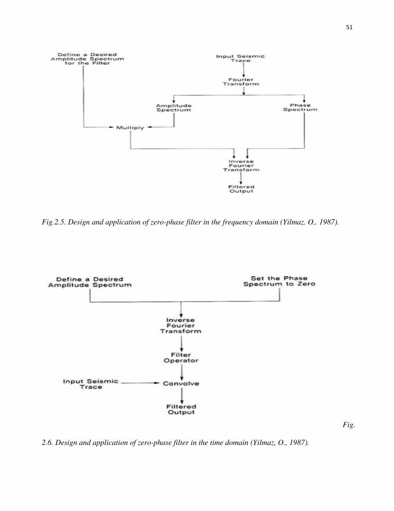
In frequency filtering, a zero-phase band limited wavelet can be used to filter a seismic trace. The

filter operator is the time domain representation of the wavelet, while the filter coefficients are the

individual time samples of this operator. The above described process is termed zero-phase frequency

filtering. It does not modify the phase spectrum of the input trace but limits the band of its amplitude

spectrum.

49

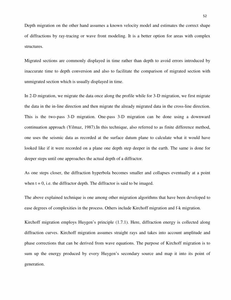
Frequency domain filtering involves multiplying the amplitude spectrum of the input seismic trace by

that of the filter operator while in the time domain. It involves convolving the filter operator with the

input time series. The summary of both frequency and time domain filtering is illustrated in figures

(2.5) and (2.6). Both formulations are based on the concept that convolution in the time domain is

equivalent to multiplication in the frequency domain and vice versa (Bracewell, 1965).

Frequency filtering could be in the form of band pass which only extracts a defined band of frequency

but does not alter its phase. Examples of frequency filters are high-pass, low-pass, band-pass and

notch frequency filters. Band-pass filters are the most used.

In velocity (f-k) filtering, the f-k plane allows us to separate events that dip in the (t,x) plane by their

dips. This consequently eliminates certain types of noise from a data. This filter suppresses coherent

linear noise arising from side-scattering energy in stacked common shot gathers.

The basis for f-k filtering is that events with the same dip in the t-x plane are mapped into a single

line in the radial direction of the f-k plane irrespective of their location on the t-x plane. This results in

the defining and application of a reject fan in the transform domain and then inverse transposing the

data back to the (t,x) domain.

F-k dip filtering is recommendably applied on shot gathers instead of CMP gathers. Its application

after stacking further suppresses noise. Likewise, coherent linear noise on stacked data can be

suppressed by post-stack migration process which also incorporates dip filtering.

2.5.10. Migration

The goal of migration is to make the stacked section as close to the geological cross-section as

possible. When displayed, the stacks appear to be a geological image. Thus, migration is also called

seismic imaging.

50

Migration is an inverse wave scattering calculation that relocates seismic reflections and diffractions

to the location of their origin, arranging data laterally in the image volume. It is inherently a 2-D or 3-

D procedure and of course, the 3-D migration produces a more accurate seismic image. Migration

operation collapses subtle diffractions associated with growth faults and also unties ‘bowties’ into

synclines.

Migration could either be pre-stack or post-stack. Pre-stack migration is recommended for survey

areas with complex structures such that each seismic trace is migrated solely before stacking.

Velocity analysis algorithms in pre-stack migration allow processors to improve their velocity models

between migration iterations. Its major disadvantage is the large data size to be migrated. Post-stack

migration involves migrating a stacked section.

Besides distinctions between 2-D versus 3-D and pre-stack versus post-stack migrations, migration

implementations are also distinguished as either time migration or depth migration.

Time migration assumes that local variations in velocity is a function of depth alone and usually

ignores the refraction that occurs when rays cross the velocity boundaries. When lateral variations are

much, time migration is not recommended, the migration algorithms for time migration are quite

simple.

51

Fig.2.5. Design and application of zero-phase filter in the frequency domain (Yilmaz. O,. 1987).

Fig.

2.6. Design and application of zero-phase filter in the time domain (Yilmaz, O., 1987).

52

Depth migration on the other hand assumes a known velocity model and estimates the correct shape

of diffractions by ray-tracing or wave front modeling. It is a better option for areas with complex

structures.

Migrated sections are commonly displayed in time rather than depth to avoid errors introduced by

inaccurate time to depth conversion and also to facilitate the comparison of migrated section with

unmigrated section which is usually displayed in time.

In 2-D migration, we migrate the data once along the profile while for 3-D migration, we first migrate

the data in the in-line direction and then migrate the already migrated data in the cross-line direction.

This is the two-pass 3-D migration. One-pass 3-D migration can be done using a downward

continuation approach (Yilmaz, 1987).In this technique, also referred to as finite difference method,

one uses the seismic data as recorded at the surface datum plane to calculate what it would have

looked like if it were recorded on a plane one depth step deeper in the earth. The same is done for

deeper steps until one approaches the actual depth of a diffractor.

As one steps closer, the diffraction hyperbola becomes smaller and collapses eventually at a point

when t = 0, i.e. the diffractor depth. The diffractor is said to be imaged.

The above explained technique is one among other migration algorithms that have been developed to

ease degrees of complexities in the process. Others include Kirchoff migration and f-k migration.

Kirchoff migration employs Huygen’s principle (1.7.1). Here, diffraction energy is collected along

diffraction curves. Kirchoff migration assumes straight rays and takes into account amplitude and

phase corrections that can be derived from wave equations. The purpose of Kirchoff migration is to

sum up the energy produced by every Huygen’s secondary source and map it into its point of

generation.

53

F-k migration uses the 2-D Fourier transform to convert the input t-x section into an f-k section.

Migration of seismic data is carried out in the frequency domain. The seismic time section is first

converted to an apparent depth section. In the apparent depth mode, a constant velocity is assigned to

all reflections. Then, this seismic data is two-dimensionally transformed into frequency and wave

number domain. The inverse 2-D FT provides the migrated t-x section

2.6. Mathematical operations in seismic data processing

Three types of mathematical operations constitute the heart of most data processing. They are Fourier

transform, convolution and correlation, however, the z-transform can be included as another

mathematical operation.

Fourier transform (FT) is used to convert from the time domain to the frequency domain and vice

versa. It can also be used alongside other transforms to convert into and out of other domains.

Convolution operation replaces each element of an input with a scaled output function. This operation

better explains the limitations placed on sampling and signal reconstitution.

Correlation is a method of measuring similarities between two data sets by determining the time shift

that will maximize such similarities. It is also used to extract short signals of known wave shape from

long train waves as used in vibroseis processing. Auto-correlation is a situation where a data is

correlated by itself and cross-correlation occurs when different data are correlated.

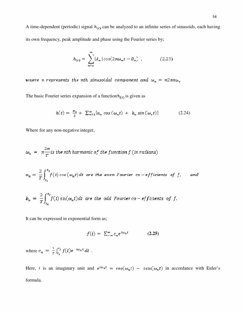
2.6.1. The Fourier series/transform

Consider a mono-frequency sinusoidal function given by

54

A time-dependent (periodic) signal can be analyzed to an infinite series of sinusoids, each having

its own frequency, peak amplitude and phase using the Fourier series by;

The basic Fourier series expansion of a function is given as

(2.24)

Where for any non-negative integer,

It can be expressed in exponential form as;

(2.25)

where

Here, is an imaginary unit and in accordance with Euler’s

formula.

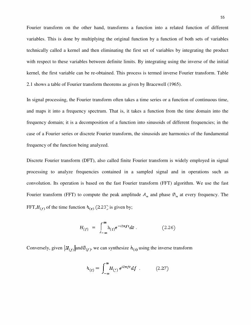
55

Fourier transform on the other hand, transforms a function into a related function of different

variables. This is done by multiplying the original function by a function of both sets of variables

technically called a kernel and then eliminating the first set of variables by integrating the product

with respect to these variables between definite limits. By integrating using the inverse of the initial

kernel, the first variable can be re-obtained. This process is termed inverse Fourier transform. Table

2.1 shows a table of Fourier transform theorems as given by Bracewell (1965).

In signal processing, the Fourier transform often takes a time series or a function of continuous time,

and maps it into a frequency spectrum. That is, it takes a function from the time domain into the

frequency domain; it is a decomposition of a function into sinusoids of different frequencies; in the

case of a Fourier series or discrete Fourier transform, the sinusoids are harmonics of the fundamental

frequency of the function being analyzed.

Discrete Fourier transform (DFT), also called finite Fourier transform is widely employed in signal

processing to analyze frequencies contained in a sampled signal and in operations such as

convolution. Its operation is based on the fast Fourier transform (FFT) algorithm. We use the fast

Fourier transform (FFT) to compute the peak amplitude and phase at every frequency. The

FFT, of the time function is given by;

Conversely, given and , we can synthesize using the inverse transform

56

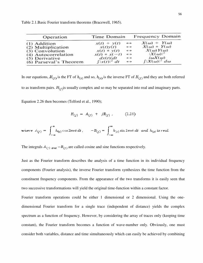
Table 2.1.Basic Fourier transform theorems (Bracewell, 1965).

In our equations, is the FT of and so, is the inverse FT of and they are both referred

to as transform pairs. is usually complex and so may be separated into real and imaginary parts.

Equation 2.26 then becomes (Telford et al., 1990);

The integrals are called cosine and sine functions respectively.

Just as the Fourier transform describes the analysis of a time function in its individual frequency

components (Fourier analysis), the inverse Fourier transform synthesizes the time function from the

constituent frequency components. From the appearance of the two transforms it is easily seen that

two successive transformations will yield the original time-function within a constant factor.

Fourier transform operations could be either 1 dimensional or 2 dimensional. Using the one-

dimensional Fourier transform for a single trace (independent of distance) yields the complex

spectrum as a function of frequency. However, by considering the array of traces only (keeping time

constant), the Fourier transform becomes a function of wave-number only. Obviously, one must

consider both variables, distance and time simultaneously which can easily be achieved by combining

57

the two one-dimensional transforms into one two-dimensional Fourier transform, giving rise to 2-D

Fourier transform. 2-D transform is the basis for both the analysis and implementation of multi-

channel processes. It is a mathematical process which basically involves transforming a set of data

from time-space domain to the frequency-wave-number domain. The two-dimensional complex

spectrum, therefore, is a function of both frequency and wave-number. 2-D transforms decompose a

wave field into its plane-wave components.

Other types of transform also exist. They are Laplace transform, Radon transform and z-transform.

Transforms and their functions are in domains specified by the variables. They are designed to

preserve information as they switch domains even though minor alterations occur due to

approximations and truncations.

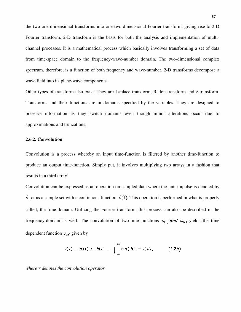
2.6.2. Convolution

Convolution is a process whereby an input time-function is filtered by another time-function to

produce an output time-function. Simply put, it involves multiplying two arrays in a fashion that

results in a third array!

Convolution can be expressed as an operation on sampled data where the unit impulse is denoted by

or as a sample set with a continuous function . This operation is performed in what is properly

called, the time-domain. Utilizing the Fourier transform, this process can also be described in the

frequency-domain as well. The convolution of two-time functions yields the time

dependent function given by

where denotes the convolution operator.

58

Convolution can be defined based on equation 2.29 as the integral of the product of the two functions

after one is reversed and shifted. As such, it is a particular kind of integral transform. The integration

range depends on the domain on which the functions are defined. Using zero-extended or infinite

domains is sometimes called a linear convolution.

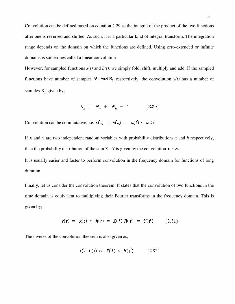
However, for sampled functions x(t) and h(t), we simply fold, shift, multiply and add. If the sampled

functions have number of samples respectively, the convolution y(t) has a number of

samples given by;

Convolution can be commutative, i.e. .

If X and Y are two independent random variables with probability distributions x and h respectively,

then the probability distribution of the sum X + Y is given by the convolution

It is usually easier and faster to perform convolution in the frequency domain for functions of long

duration.

Finally, let us consider the convolution theorem. It states that the convolution of two functions in the

time domain is equivalent to multiplying their Fourier transforms in the frequency domain. This is

given by;

The inverse of the convolution theorem is also given as,

59

2.6.3. Correlation

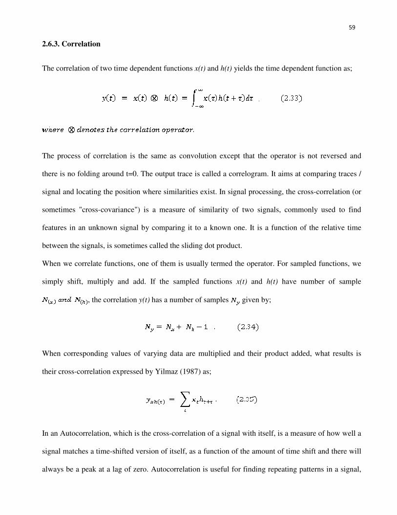
The correlation of two time dependent functions x(t) and h(t) yields the time dependent function as;

The process of correlation is the same as convolution except that the operator is not reversed and

there is no folding around t=0. The output trace is called a correlogram. It aims at comparing traces /

signal and locating the position where similarities exist. In signal processing, the cross-correlation (or

sometimes "cross-covariance") is a measure of similarity of two signals, commonly used to find

features in an unknown signal by comparing it to a known one. It is a function of the relative time

between the signals, is sometimes called the sliding dot product.

When we correlate functions, one of them is usually termed the operator. For sampled functions, we

simply shift, multiply and add. If the sampled functions x(t) and h(t) have number of sample

, the correlation y(t) has a number of samples given by;

When corresponding values of varying data are multiplied and their product added, what results is

their cross-correlation expressed by Yilmaz (1987) as;

In an Autocorrelation, which is the cross-correlation of a signal with itself, is a measure of how well a

signal matches a time-shifted version of itself, as a function of the amount of time shift and there will

always be a peak at a lag of zero. Autocorrelation is useful for finding repeating patterns in a signal,

60

such as determining the presence of a periodic signal which has been buried under noise, or

identifying the missing fundamental frequency in a signal implied by its harmonic frequencies.

If X and Y are two independent random variables with probability distributions x and h, respectively,

then the probability distribution of the difference − X + Y is given by the cross-correlation of f and g.

In contrast, the convolution, x * h, gives the probability distribution of the sum X + Y.

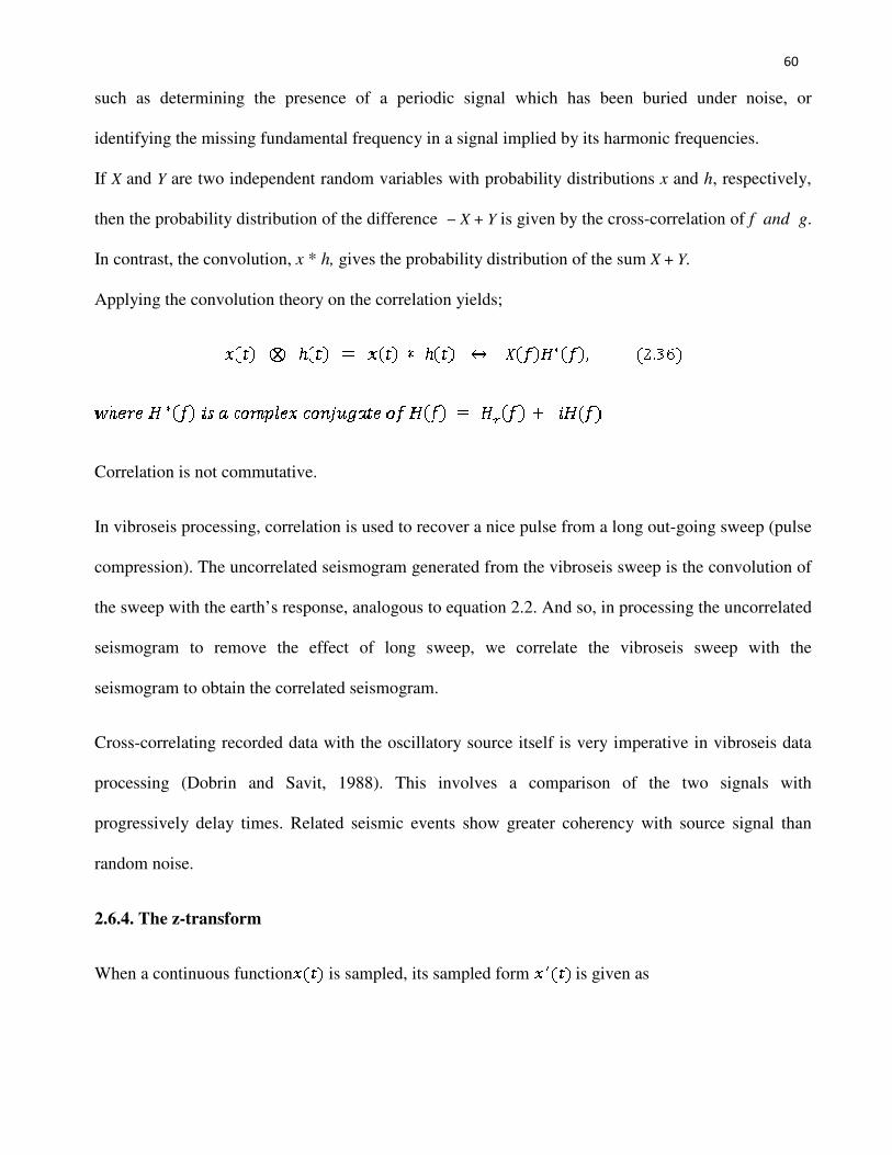
Applying the convolution theory on the correlation yields;

Correlation is not commutative.

In vibroseis processing, correlation is used to recover a nice pulse from a long out-going sweep (pulse

compression). The uncorrelated seismogram generated from the vibroseis sweep is the convolution of

the sweep with the earth’s response, analogous to equation 2.2. And so, in processing the uncorrelated

seismogram to remove the effect of long sweep, we correlate the vibroseis sweep with the

seismogram to obtain the correlated seismogram.

Cross-correlating recorded data with the oscillatory source itself is very imperative in vibroseis data

processing (Dobrin and Savit, 1988). This involves a comparison of the two signals with

progressively delay times. Related seismic events show greater coherency with source signal than

random noise.

2.6.4. The z-transform

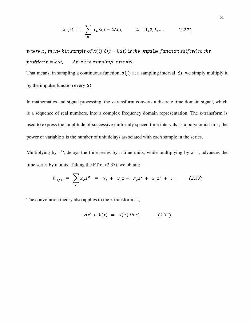
When a continuous function is sampled, its sampled form is given as

61

That means, in sampling a continuous function, at a sampling interval , we simply multiply it

by the impulse function every .

In mathematics and signal processing, the z-transform converts a discrete time domain signal, which

is a sequence of real numbers, into a complex frequency domain representation. The z-transform is

used to express the amplitude of successive uniformly spaced time intervals as a polynomial in ; the

power of variable z is the number of unit delays associated with each sample in the series.

Multiplying by , delays the time series by n time units, while multiplying by , advances the

time series by n units. Taking the FT of (2.37), we obtain;

The convolution theory also applies to the z-transform as;

62

CHAPTER THREE

LITERATURE REVIEW

3.1. Introduction

The seismic reflection method is a method of exploration geophysics that uses the principles of

seismology to estimate the properties of the earth’s sub-surface from seismic reflected waves. This

method is mainly directed at locating depths of reflecting surfaces and the seismic velocities of sub-

surface rock layers. It is mainly used for hydrocarbon and mineral exploration due to its ability to

penetrate deep into the earth, up to several hundred meters. Over the years, this method has been

developed to quite a high degree of sophistication.

The method requires a controlled source of energy or signal, usually an explosion or vibration, sent

into the ground at a known time and location. By taking note of the time it takes the signal to be

reflected back from the boundaries between rocks to a receiver on the earth’s surface (usually a

geophone for land and a hydrophone for marine), the depths and features of the sub-surface interfaces

can be estimated after some processing and analyses.

Several field procedures are in use, each being distinguished by the different layout of the detectors

relative to the shot-point.

This report reviews ten (10) reflection operations carried out in different parts of the world, at

different times and for different purposes. The choice of the cases reviewed in this work was carefully

and thoughtfully arrived at. This is to enable a better comparison of data acquisition parameters,

equipment used and the different approaches to data processing and interpretation.

63

The cases reviewed in this report are: Seismic reflection studies in the Skellefte Ore district. Northern

Sweden, Seismic reflection tomography: A case study of a shallow lake in Lake Balaton, COCORP’S

deep seismic reflection profiling in the Williston Basin (comparison of explosive and vibroseis source

energy penetration), Reflection seismic and ground-penetrating radar: Study of previously mined

(lead/zinc) ground, Joplin, Missouri, Seismic processing and velocity assessments in the oil and gas

resource potential of the 1002 area, Arctic National Wild Life Refuge (ANWR), Alaska, Seismic

reflection investigation of C-1 to F-1 sector of the Superconducting Super Collider (SSC) ring west of

Waxahachie, Texas, Analysis of existing seismic reflection data in South Florida for Aquifer Storage

and Recovery (ASR) regional study, 4D acquisition using two boats in the Enfield oil field offshore,

Western Australia,3D interpretation of the Espoir field area, offshore Ivory Coast and Structural and

stratigraphic mapping of Emi field, offshore Niger Delta, Nigeria.

.

3.2. Case 1: Seismic Reflection Studies in the Skellefte Ore District, Northern Sweden

Several world class mines are located in the western part of the Skellefte Ore district, for instance, the

Kristineberg VMS mine. The Skellefte district is a volcanic arc which formed betweena sedimentary

basin (Bothnian Basin) and a continental basin (the Aindsjaur group)(Weihed, 2001). Today,the area

is freely defined (150 by 150km in size) in Northern Vasterbotten and southern Norbotten in the

Northern part of Sweden. The area is rich in mineral occurrence. The surface geology in the

Kristineberg area consists of volcanic rocks overlain by fine-grained turbiditic metasediments.

Data was obtained in this area along two north-south oriented profiles (profiles 1 and 5) between late

August and early September, 2003 (fig. 3.1). Each data was about 25km long.

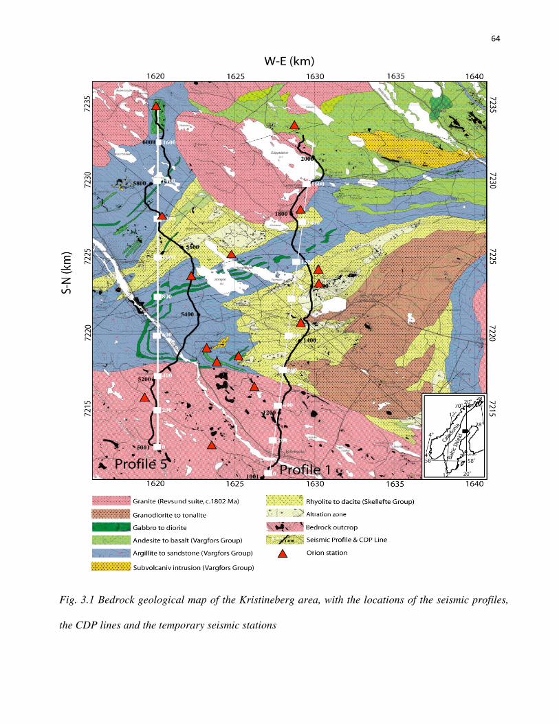
64

Fig. 3.1 Bedrock geological map of the Kristineberg area, with the locations of the seismic profiles,

the CDP lines and the temporary seismic stations

65

The purpose of the survey was to obtain high resolution images of the upper10km of the crust. The

aim of the survey was to study the very complex crustal architecture of the region in the Skellefte Ore

district in the Kristineberg area at depth and to determine the relationship between the submarine ore

bearing Skellefte group and the overlying volcanic and sedimentary rocks south of the Archean-

Proterozoic boundary. Barret and Maclean (2000) has more details on the geology of this area.

Profile 1 was first decided to run parallel to the major tectonic ligaments of the region. The profile

passed on top of the Kristineberg mine and crossed the exposed ore-bearing volcanic units of the

Vargfors group (coarse clastic unit of a sedimentary sequence).

Profile 5 was mainly located along very small roads or sections through rough terrains and runs

parallel to profile 1. This choice was due to lack of infrastructure in the east-west direction and its

ability to allow cross-profile recordings to help correlate observed structures between the profiles.

The separation between both profiles was about 6-8km. Both profiles started in the Revsund granites

in the south, crossed the ore-bearing Vangfors formation and ended in/near the Revsund granites

bordering the Skellefte field to the north (Tryggvason et al., 2003).

Data acquisition:

The 3D reflection survey was conducted within an interval of approximately 3 weeks. Two data

recording systems were used, the SERCEL 348 and SERCEL 408. SERCEL 348, which is an older

version is heavier and more strenuous in rough terrains, was used for profile 1. Also for profile 1, a

group of six 10Hz geophones was used. The more modern SERCEL 408 was used for profile 5

alongside single 28Hz geophones. A summary of the acquisition parameters are shown in table 3.1.

An alternative source of a vibratory system was contemplated but the idea discarded due to very high

mobilization costs. Recording started at the southern ends of the profiles. Data was recorded on

66

temporal seismometers spread out in the area to 20s and sampled every 2ms. GPS instruments used

ensured high precision of shot-hole and geophone locations.

Processing:

PROMAX was the processing package used to process the data which was done at the Department of

Earth Science, Uppsala University. Though recording was done for 20s TWT, processing was done to

4s TWT only (about 12km depth). Similar processing schemes were used for both profiles. Editing

was done in shot domain to remove cultural traffic and ambient noise. Processing sequences applied

to the data are summarized in table 3.2.

Some data on profile 5 were corrected for reverse polarity. First arrivals were picked with an

automatic neutral network algorithm and proper correction effected where necessary after manual

inspection.

3.3. Case 2: Seismic Reflection Tomography: A Case Study of a Shallow Lake in Lake Balaton.

Lake Balaton is the largest lake in Central Europe. It is situated near Budapest in Hungary and is

home to precious natural treasures (fig. 3.2). Lake Balaton is 77km in length and has a width range of

4-14km. Near surface material of the lake consists of unconsolidated, medium to coarse-grained mud

and medium to coarse gravel interspaced with thin discontinuous Paleosols and clay. Test hole of

seismic section in the area indicates a thick Holocene mud layer (3.5 – 4m thick) present just below

the water and a stiff saturated clay stratum just below it (McLamore et. al., 1978).

67

Fig. 3.2. Location map of the broader study area of Lake Balaton.

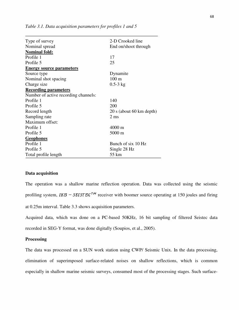
68

Table 3.1. Data acquisition parameters for profiles 1 and 5

Type of survey 2-D Crooked line

Nominal spread End on/shoot through

Nominal fold:

Profile 1 17

Profile 5 25

Energy source parameters

Source type Dynamite

Nominal shot spacing 100 m

Charge size 0.5-3 kg

Recording parameters

Number of active recording channels:

Profile 1 140

Profile 5 200

Record length 20 s (about 60 km depth)

Sampling rate 2 ms

Maximum offset:

Profile 1 4000 m

Profile 5 5000 m

Geophones

Profile 1 Bunch of six 10 Hz

Profile 5 Single 28 Hz

Total profile length 55 km

Data acquisition

The operation was a shallow marine reflection operation. Data was collected using the seismic

profiling system, receiver with boomer source operating at 150 joules and firing

at 0.25m interval. Table 3.3 shows acquisition parameters.

Acquired data, which was done on a PC-based 50KHz, 16 bit sampling of filtered Seistec data

recorded in SEG-Y format, was done digitally (Soupios, et al., 2005).

Processing

The data was processed on a SUN work station using CWP/ Seismic Unix. In the data processing,

elimination of superimposed surface-related noises on shallow reflections, which is common

especially in shallow marine seismic surveys, consumed most of the processing stages. Such surface-

69

related noises which include direct waves, guided waves, water bottom multiples, reflected refractions

and side scattered noise (Lee, 1999).

Table3.2. A summary of the processing operations on profiles 1 and 5

Read SEG format files 20,000 ms

Reverse negative polarities in

first breaks Profile5 only

Spike and noise edit Both profiles

Pick first breaks Both profiles

Refraction statics

Profile 5: 240 m datum, 1 layer model, 5700 m/s replacement vel.

Profile 1: 300 m datum, 1 layer model, 5500 m/s replacement vel.

Spectral Whitening Profile 1: Time-variant

Profile 5: 10,20,75,105 Hz

Band-pass filtering Profile 1: Time & space-variant

Profile 5: 20-40-70-120 Hz, 0-4000 ms

Air blast attenuation Profile 5 only

Sort to CMP domain Both profiles

Velocity analysis Both profiles

NMO correction 40% stretch mute

Residual statics, maximum power autostatics, pass1

Velocity analysis

Residual statics, maximum power autostatics, pass2

Stacking Both profiles

F-X Deconvolution Both profiles

Time-variant scaling Profile 1

Trace equalization Profile 5

Processing tools applied on the data include band-pass filtering, mute (windowing), f-k filtering,

spectrum analysis, gain deconvolution and migration. Velocity analysis was not possible because of

the single fold nature of the survey, however, a tomographic approach of the model using reflection

travel-times from the pre-defined reflectors was attempted to tackle that issue. In this case, a 5-

layered, 1D background velocity extracted from a bore-hole in the vicinity of the seismic section was

used. The forward model was solved using finite-difference wave equation modeling.

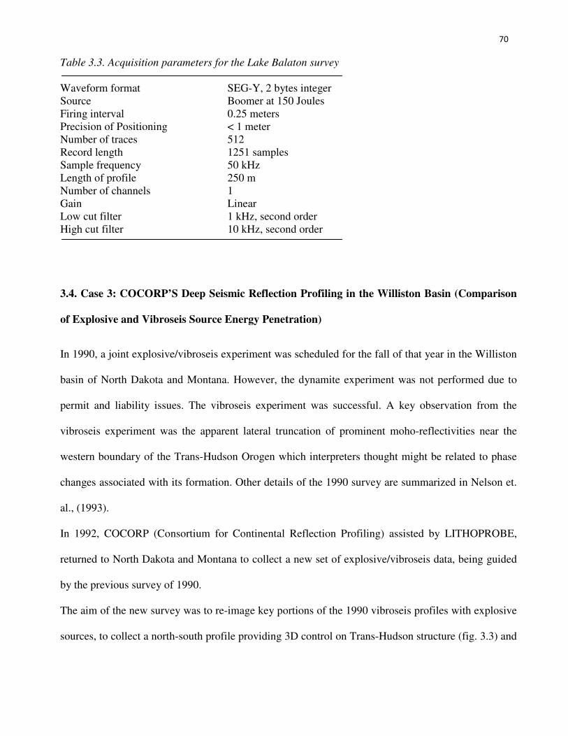
70

Table 3.3. Acquisition parameters for the Lake Balaton survey

Waveform format SEG-Y, 2 bytes integer

Source Boomer at 150 Joules

Firing interval 0.25 meters

Precision of Positioning < 1 meter

Number of traces 512

Record length 1251 samples

Sample frequency 50 kHz

Length of profile 250 m

Number of channels 1

Gain Linear

Low cut filter 1 kHz, second order

High cut filter 10 kHz, second order

3.4. Case 3: COCORP’S Deep Seismic Reflection Profiling in the Williston Basin (Comparison

of Explosive and Vibroseis Source Energy Penetration)

In 1990, a joint explosive/vibroseis experiment was scheduled for the fall of that year in the Williston

basin of North Dakota and Montana. However, the dynamite experiment was not performed due to

permit and liability issues. The vibroseis experiment was successful. A key observation from the

vibroseis experiment was the apparent lateral truncation of prominent moho-reflectivities near the

western boundary of the Trans-Hudson Orogen which interpreters thought might be related to phase

changes associated with its formation. Other details of the 1990 survey are summarized in Nelson et.

al., (1993).

In 1992, COCORP (Consortium for Continental Reflection Profiling) assisted by LITHOPROBE,

returned to North Dakota and Montana to collect a new set of explosive/vibroseis data, being guided

by the previous survey of 1990.

The aim of the new survey was to re-image key portions of the 1990 vibroseis profiles with explosive

sources, to collect a north-south profile providing 3D control on Trans-Hudson structure (fig. 3.3) and

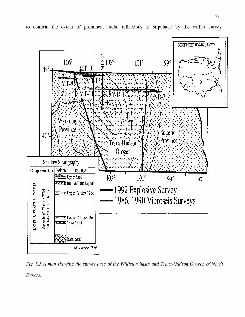
71

to confirm the extent of prominent moho reflections as stipulated by the earlier survey.

Fig. 3.3 A map showing the survey area of the Williston basin and Trans-Hudson Orogen of North

Dakota.

72

Another objective of the survey was to test the feasibility of using explosive source in low-fold mode

for deep reflection profiling. The objective of this survey which is of the most interest in this review

is the comparison in the effective imaging of deep structures between the 1990 vibroseis survey and

the 1992 explosive survey.

Data acquisition

Three explosive data were collected in the Williston basin in the 1992 survey; MT12, ND2 and ND3,

each having its own objective. MT12 was designed to test the moho-reflectivity, ND2 was collected

to confirm the along-strike correlation of primary crustal fabrics as suggested by comparison of the

COCORP’s data with subsequent LITHOPROBE surveys in the Saskatchewan to the north (Baird,

1995) and ND3 was acquired to extend imaging further into the bounding superior craton east of the

Trans-Hudson Orogen.

A total of 129 shots were taken for MT12, ND2 and ND3 surveys, of which 97 shots were used to

study shot-to-shot variability. A high fold (30) data was acquired for the vibroseis data while a low

fold (6) data was obtained for the explosive data.

For the 1992 explosive survey, multiple DFS V systems, each equipped with 120 channels recording

system was used. Explosive sources were positioned with a nominal 3km spacing. Explosive shots

varied (from 9.5-90kg) with depths varying from22-38m (140-180ft). This was due to shots being

placed in different media (clay, sand, shale and sand stone). The MT12 survey was shot from west to

east (fig. 3.3) with multiple DFS V systems used in-line to create a 24-30km spread. Nine (9)

L21A(10Hz) geophone was used as detectors.

For the vibroseis survey of 1990, Amoco’s 600+ channel telemetric recording system using radio-

linked seismic group recorders deployed in a roll-along configuration was used. The source

comprised eight (8) Mertz vibrators [52,000 lb (23,000N) peak force P-wave] positioned bumper to

bumper to form a 40m in-line linear array. The source array was moved one pad length per sweep

73

with vibration points every 200m. Twelve (12) SM-7 (10Hz) geophones acted as detectors per station.

Production shots for ND2 and ND3 used 45kg of explosive in two shot holes with a separation of

85m.

Processing

It is clearly obvious that the geometries, equipment and processing procedures for both data were

different in every sense. Another major difference was the two years interval separating both

operations. As a result, no quantitative or definitive comparison could be made on both data.

However, given that eleven (11) points from the approximately 35km of vibroseis and explosive data

overlapped on both the western and eastern portions of the transect MT10/12 and ND1-ND3, an

analysis became useful and necessary. Data in the overlapped region included shots and receivers

placed in both surface media (Steer et al., 1996).

Since the acquisition and time of acquisition of both data sets were different, both data were

normalized to minimize amplitude variations caused by the effect of varying ambient noise conditions

and were sealed to reduce synthetic biases which resulted from the use of different recording systems

and geophone patterns. The amplitude normalization was done by taking the absolute amplitude of

samples from the eleven coincident channels centered at 4km (a distance thoughtfully chosen),

summing them up to a single channel and then calculating the RMS amplitudes for selected 100ms

windows from 2-50 TWT.

The correlation process left the vibroseis data bandwidth limited. Although no much difference will

be noticed if the explosive data was band-pass filtered to match the vibroseis bandwidth.

74

3.5. Case 4: Reflection Seismic and Ground-Penetrating Radar Study of Previously Mined

(Lead/Zinc) Ground, Joplin, Missouri.

The Missouri Department of Transport (MoDOT) proposed constructing an inter-state route Alternate

“E” across the Joplin area of Missouri (fig. 3.4). The site had been previously mined for Lead/Zinc

and had been extensively open-pit and so the integrity of the ground became a thing of concern. In the

winters of 1996/1997 and 1997/1998, the MoDOT contracted the departments of Geology and

Geophysics at the University of Missouri-Rolla to conduct a geophysical survey on the entire area to

ascertain the condition of the ground.

The survey had the following objectives;

1. To map the Mississippian bedrock

2. To identify and Paleosinkholes and abandoned mine features

3. To determine the structural geologic trends in the area

4. To identify major bedrock faults and/or fracture zones

5. To identify and locate abandoned mine access and ventilation shafts overlain by surficial

milled ore rock.

The applicability of these objectives was primarily to aid MoDOT engineers involved in route

planning, hazard assessment and site mitigation. To achieve this, the University of Missouri-Rolla

conducted two geophysical surveys on the area; a reflection survey to investigate objectives 1- 4

above and a ground-penetrating radar (GPR) survey to attempt achieving the fifth objective.

75

Fig 3.4. Map of the survey area in Joplin, Missouri.

76

Data acquisition

A total of 14,600 lineal meters of shallow reflection seismic data, 15,000 lineal meters of GPR data

and 9 down-hole seismic calibration check-shots were acquired.

An elastic wave generator weight drop was used as source while single channel 40Hz geophones

served as detectors. Seismic reflection data was acquired using a 24-channel Bison Engineering

seismograph with roll-along capabilities. Weight drop source was impacted 6-14 times per shot

record. An interval of 3m was employed for shot, receiver and near-offset spacings. Data processing

was on a Pentium PC using WINSEIS.

Data processing

Processing steps applied to the seismic data include reflection identification from bedrock, muting of

all arrivals prior to bedrock event, first breaks and ground rolls, restoration of shot-gather traces to

CMP gathers, elevation correction, velocity analysis for each line, calculation and application of

surface consistent statics, NMO correction, stacking, residual statics, re-stacking statically corrected

data and band-pass filtering (Shoemaker et al., 2000).

To provide sub-surface lithologic/velocity control and to confirm the interpretation of the reflection

data, MoDOT drilled 23 bore-holes in the area but down-hole calibration check-shot survey data was

acquired at 9 bore-hole locations. Surface to bore-hole tomography was applied with a spacing of 1m.

The check-shot data acquired was used to determine P-wave time-depth and velocity time-depth

relationships for shallow sub-surfaces.

For the GPR profiling, a Geophysical Survey System Inc. sub-surface interface radar unit (SIR-8)

equipped with a 500MHz monostatic antenna was used. A total of 1,500 lineal meters of GPR data

was obtained. The data was acquired as suites of parallel GPR profiles with a separation of 1.5m.

Sampling interval was 30scans/foot and trace length was 100ns.

77

The GPR was processed on a Pentium PC using RADAN. Processing operation applied to the data

include trace normalization, vertical gain application, horizontal and vertical filtering.

3.6. Case 5: Seismic Processing and Velocity Assessments in the Oil and Gas Resource Potential

of the 1002 AREA, Arctic National Wild Life Refuge (ANWR), Alaska.

The Geophysical Service Inc. (GSI), under a contract to a consortium of petroleum exploration

companies in 1984 and 1985, acquired and processed 1,451mi (2,351km) of multi-channel seismic

data on and adjacent to the Arctic National Wildlife Refuge (ANWR). That was part of a petroleum

resource evaluation study which was later performed in 1987 by the Fish and Wildlife Service (FWS),

The Bureau of Land Management (BLM) and the US Geological Survey (USGS). Details of this

evaluation can be seen in (Bird and Magoon, 1987).

At that time in 1987, the USGS reprocessed a part of the seismic data on a VAX11/780 computer

using the DIGICON, Inc., DISCO software package. The reprocessed section was stacked and

intended for use as illustration in the resource assessment publication of 1987.

A renewed interest as to the amount of petroleum that could be buried beneath the ANWR coastal

plain led to a re-evaluation of the resource potential and a re-processing of the 1984/1985 seismic data

with a more modern and more sophisticated workstation in 1996. It was done on a SUN workstation

using PROMAX processing software developed by Landmark, Inc., together with in-house developed

software. This project started in 1996 and the processing was performed on a SUN SPARC Station2

but in August, 1997, the system was upgraded to a SUN ULTRA1because the latter was fast enough

to run some testing of pre-stack depth migration (Lee et al., 1999).

Data acquisition

982.7km (606.6mi) of seismic reflection data using dynamite sources and 247.1km (152.5mi) using

vibroseis source was acquired by GSI from January, 1984 to April 1984. In 1985, another 1121.5km

(692.3mi) seismic reflection data using vibroseis source only was obtained by GSI. A summary of the

78

recording parameters for both dynamite and vibroseis data is shown on table 3.4. Notice the change in

vibroseis sweep for both years and also the change in correlation time.

Data processing

Firstly, the rest of the data was demultiplexed from SEG-B to SEG-Y format and then the geometry

was defined and data stored from shot gather to CMP gathers. At that stage also, the elevation and up-

hole times or depths were stored in the data base.

A two-window spiking deconvolution with operator lengths of about 180ms was applied to both

dynamite and vibroseis data. That was done to improve temporal resolution. A minimum phase

deconvolution was applied to the dynamite data and a zero-phase deconvolution applied to the

vibroseis data. To correct for elevation, a floating datum was determined. By that floating datum,

elevation statics was computed and applied to individual traces.

F-k filtering was applied on shot domain only even though receiver domain f-k filtering was used in

certain parts of some profiles as an option to improve stack quality. F-k filtering suppresses linear

move-out events and improves S/N ratio significantly.

NMO correction using an automatic stretch with a maximum percentage of stretch of about 20% was

then applied to the data.

3.7. Case 6: Seismic Reflection Investigation of C-1 to F-1 Sector of the Superconducting Super

Collider (SSC) Ring West of Waxahachie, Texas.

Between 19th

June and 29th

June, 1990, LCT Houston and its sub-contractor, Dobecki Earth Science

(DES) performed a seismic reflection survey along a 16,600ft segment of the SSC, ring west of

Waxahachie (fig. 3.5). The contract was awarded to them by The Earth Technology Corporation

(TETC). That survey followed an earlier feasibility survey carried out some one mile south of the

present survey area in February of the same year (LCT, 1990).

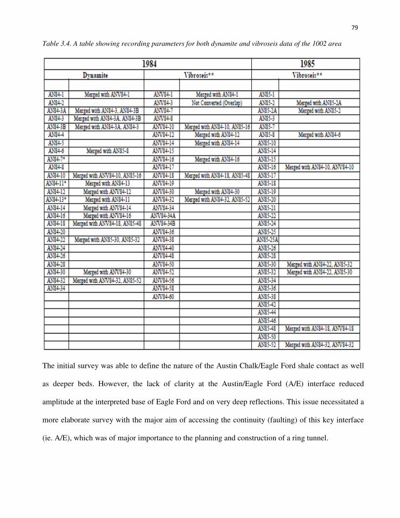
79

Table 3.4. A table showing recording parameters for both dynamite and vibroseis data of the 1002 area

The initial survey was able to define the nature of the Austin Chalk/Eagle Ford shale contact as well

as deeper beds. However, the lack of clarity at the Austin/Eagle Ford (A/E) interface reduced

amplitude at the interpreted base of Eagle Ford and on very deep reflections. This issue necessitated a

more elaborate survey with the major aim of accessing the continuity (faulting) of this key interface

(ie. A/E), which was of major importance to the planning and construction of a ring tunnel.

80

From the earlier feasibility survey, depth to the A/E contact was of the order of 200ft. the thickness of

soils over chalk in the area was much thinner. Typical soil thickness was about 2 inches only, even

though thicker soil and deeper Austin weathering were encountered in some deeper ravines along

several check runs. Surface materials included grass fields, corn fields, treed thickets and water in

cattle stock pond.

The latter survey was decided on to be executed in a similar fashion as the previous. That means same

acquisition, source/receiver type, instrumentation, CDP fold and processing parameters. But due to

the thin nature of the soil coupled with the dry nature of the soil (temperature was typically in excess

of F), a sledge hammer source was opted for as opposed to the use of ‘Buffalo gun’ source as on

the previous survey. Another reason for this choice was based on the initial noise survey and periodic

comparisons made during the production phase. However, in areas like the northern third of the line

with heavy trees and steep under-growth, a Buffalo gun source was used since it did not require

swinging.

Data acquisition

Data was acquired using a 24-channel seismograph for recording, single 40Hz geophones for

detectors and a sledge hammer (nine stacked sledge hammer blows on a steel plate) as source. Shots

were taken at a distance 60ft from geophone points, geophone spacing was 10ft and consecutive shots

were fired at 20ft interval. The acquired data had a 600% coverage.

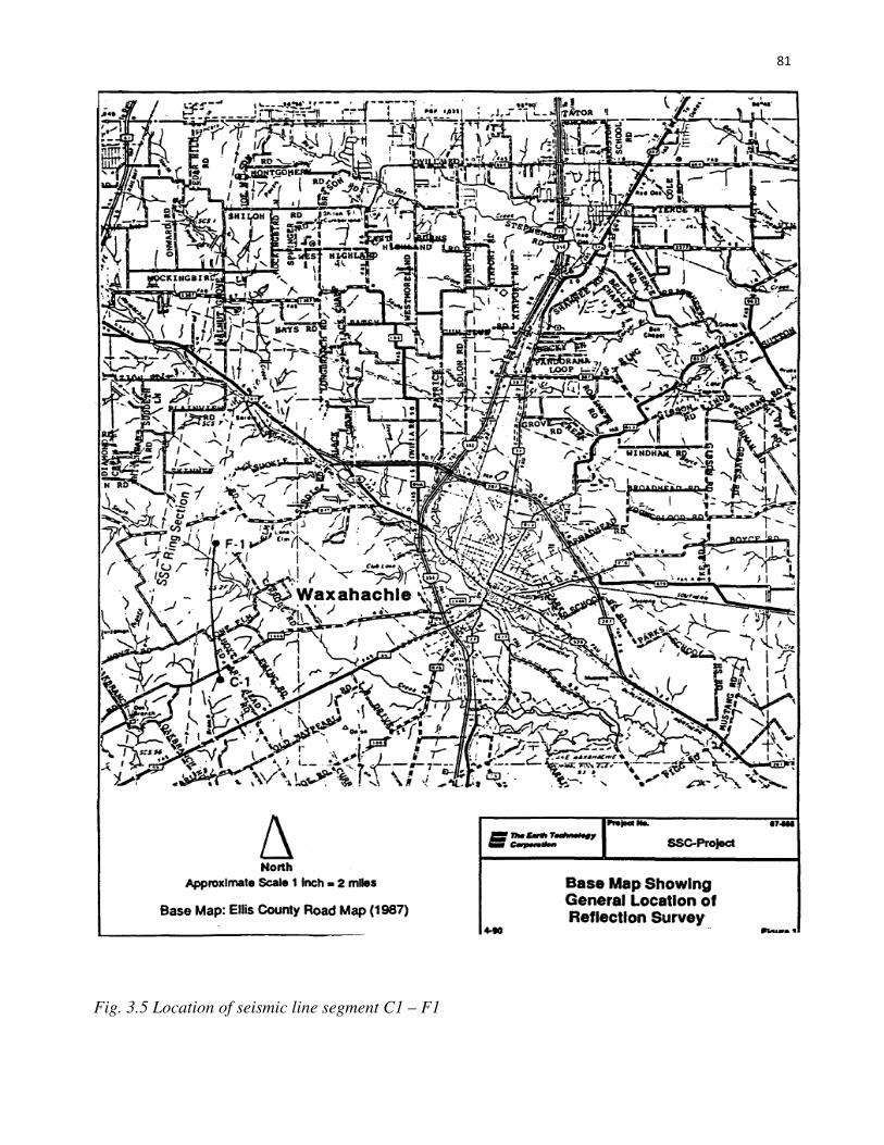
81

Fig. 3.5 Location of seismic line segment C1 – F1

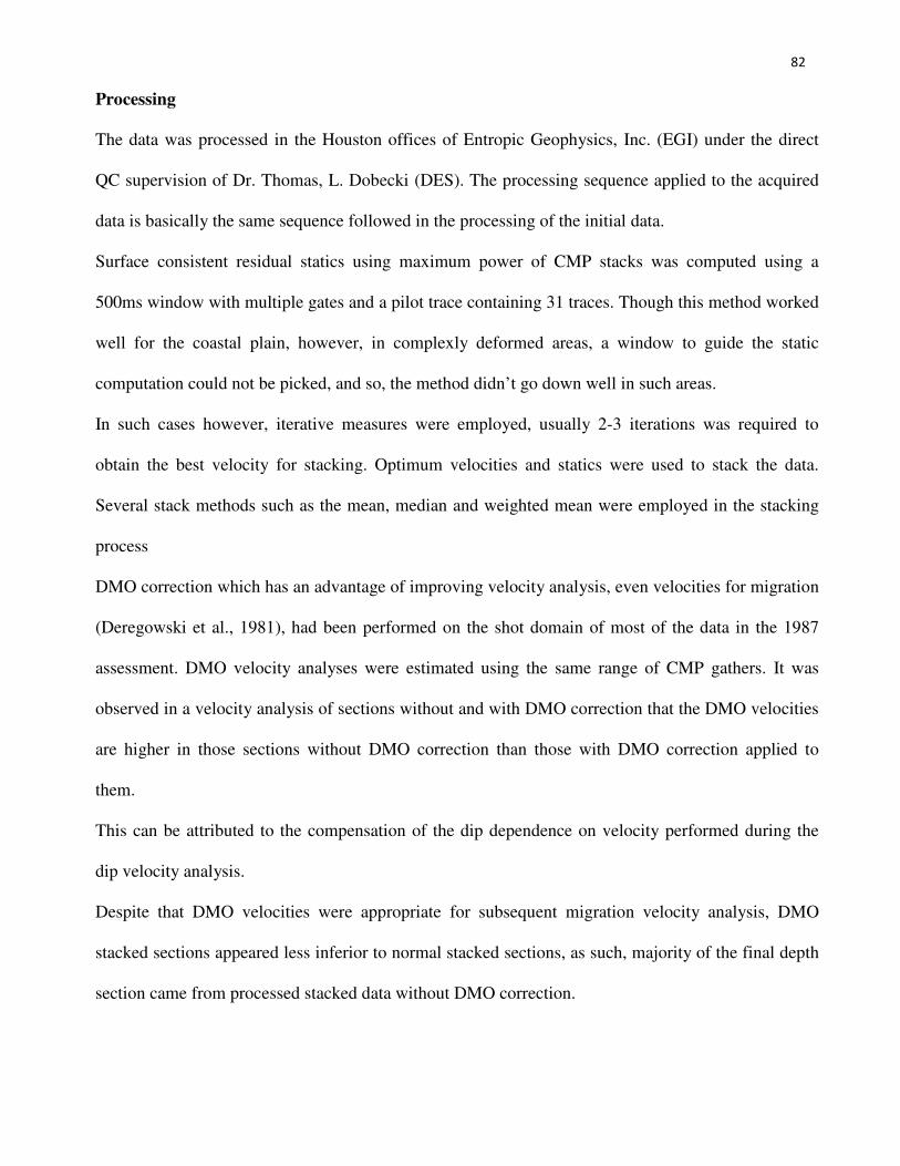
82

Processing

The data was processed in the Houston offices of Entropic Geophysics, Inc. (EGI) under the direct

QC supervision of Dr. Thomas, L. Dobecki (DES). The processing sequence applied to the acquired

data is basically the same sequence followed in the processing of the initial data.

Surface consistent residual statics using maximum power of CMP stacks was computed using a

500ms window with multiple gates and a pilot trace containing 31 traces. Though this method worked

well for the coastal plain, however, in complexly deformed areas, a window to guide the static

computation could not be picked, and so, the method didn’t go down well in such areas.

In such cases however, iterative measures were employed, usually 2-3 iterations was required to

obtain the best velocity for stacking. Optimum velocities and statics were used to stack the data.

Several stack methods such as the mean, median and weighted mean were employed in the stacking

process

DMO correction which has an advantage of improving velocity analysis, even velocities for migration

(Deregowski et al., 1981), had been performed on the shot domain of most of the data in the 1987

assessment. DMO velocity analyses were estimated using the same range of CMP gathers. It was

observed in a velocity analysis of sections without and with DMO correction that the DMO velocities

are higher in those sections without DMO correction than those with DMO correction applied to

them.

This can be attributed to the compensation of the dip dependence on velocity performed during the

dip velocity analysis.

Despite that DMO velocities were appropriate for subsequent migration velocity analysis, DMO

stacked sections appeared less inferior to normal stacked sections, as such, majority of the final depth

section came from processed stacked data without DMO correction.

83

A post-stack wavelet deconvolution was applied to all stacked data to correct for differences in source

types and to increase resolution. Prior to the post-stack wavelet deconvolution, a 1,000ms AGC was

applied to the data using a window with operator length 180ms.

A variable norm deconvolution method developed by Gray, (1979) was applied in the wavelet

processing. Different norms, window length and design area were employed in estimating wavelet

between 200 and 1,000ms in the stacked data. About 200 random windows were selected. A single

deconvolution operator was derived from the optimum parameters and applied to the whole line. A

datum correction using simple static shifts, corrected the data to a final flat datum (sea level).

Filtering was done using a band-pass filter with 8-10-68-92 Hz pass-band.

Migration of stacked data was done using Stolt’s wave –number frequency domain migration method.

The method employed migration velocity models derived from the DMO stacking velocities. Pre-

stack depth migration was performed on the data and this produced a clearer image as seen in figure

14, particularly at 10,000ft on the right side of the section.

Depth conversion of the unmigrated data was done using average velocities strictly derived from the

DMO velocities. No well data or VSP data was available in the area to tie to the reflection data.

Velocities were modified where necessary in ascertaining the validity of depth sections. Although the

converted depth section, due to lack of well or VSP data, may lack full certainty, the obtained depth

sections were geologically accurate.

To enhance the visibility of seismic reflections in the data, a 8-12-56-68Hz pass-band was applied by

a median filter using a 3 by 3 grid and their amplitudes were modulated by the trace envelope as

illustrated by Lee et. al.,(1988).

Migration velocity was derived by smoothing DMO velocities using triangular tapers in time and

space. A 300 CMP was used as the half height of a triangular smoother in space and a 500ms was

used as the half height of a triangular smoother with time. Modification of migration velocity was

84

carried out where necessary. Its average velocity was derived using smooth gradient function with the

migration velocity as its input.

3.8. Case 7: Analysis of Existing Seismic Reflection Data in South Florida for Aquifer Storage

and Recovery (ASR) Regional Study.

Several reflection lines are known to exist near and south of Lake Okeechobee in South Florida. Most

of which were collected for oil exploration purposes at depths of about 10,000-14,000ft below ground

surface.

To restore the ecosystem in that region, the Comprehensive Everglades Restoration Plan (CERP)

came up with several projects, one of which was the ASR studies. The ASR studies project was

designed to evaluate the viability and potential effects of constructing about 333 ASR wells in the

area. To do this, a better sub-surface characterization of the area which will optimize effective

location of the ASR became expedient.

Given the numerous seismic lines that traverse the area, a question on the possibility of re-processing

selected portions of available deep reflection data to resolve shallow sub-surface stratigraphy in an

area south of Lake Okeechobee was considered.

In that regard, the US Army Corps of Engineers – Jacksonville district (USACE) teaming up with the

South Florida Water Management District (SFWMD), contracted the URS Group Inc. to review the

assessment in line with CERP’s project.

A seismic data coverage map was obtained from Seismic Exchange Inc. (SEI) for a large area of

Florida. After extensive considerations of the numerous lines on the data, two 5-mile sections, one for

each of the selected lines were chosen. One of the lines utilized a dynamite source with an east-west

orientation and the other utilized a vibroseis south with the same east-west orientation. The selected

85

seismic data were 2D seismic lines acquired in the mid to late 1980s by SEI, both of which targeted

petroleum in very deep zones.

Data acquisition

A total of 399 inputs were recorded for the dynamite line and 179 recorded for the vibroseis line.

CMPs for the dynamite line were 1,157 and 1,055 for that of the vibroseis. The acquisition parameters

for both lines are shown in table 3.5.

Processing

Processing operations applied to the data include demultiplexing of data and converting it to internal

Focus format, trace editing, geometry definition, spherical divergence correction and application of

surface consistent gain. Other processing operations performed on the data are stated in table 3.5.

No elevation data was available for the vibroseis line and so elevations were estimated to be 20ft

MSL at all point. Additional corrections to the data in the CMP domain were done using residual

static programs.

The final migrated stack had a technique known as XFreq applied to it. XFreq is a program designed

by Tricon to boost amplitudes of the higher frequency range thus, enhancing the frequency content of

the data. Its principle is based on dipole filtering. Colton and Nautiyal, (1996) deals more on its

operation.

3.9. Case 8: 4D Acquisition Using Two Boats in the Enfield Oil Field Offshore, Western

Australia.

In 2004, Woodside acquired a baseline seismic data using one boat and dual sources. At the time,

water depth was about 500m and the streamer configuration was 6 by 100m. The data obtained had

good quality with a usable bandwidth of 15-80Hz and the TWT at a target level of 2s. The survey

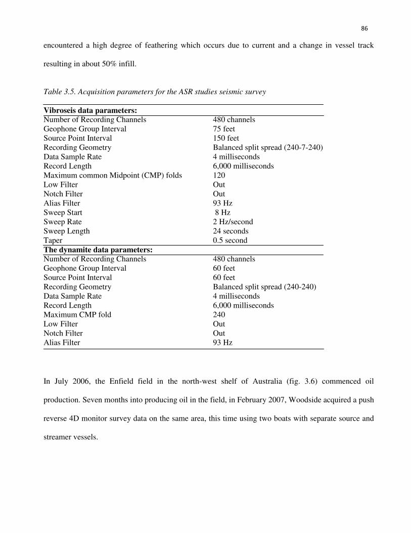
86

encountered a high degree of feathering which occurs due to current and a change in vessel track

resulting in about 50% infill.

Table 3.5. Acquisition parameters for the ASR studies seismic survey

Vibroseis data parameters: Number of Recording Channels 480 channels

Geophone Group Interval 75 feet

Source Point Interval 150 feet

Recording Geometry Balanced split spread (240-7-240)

Data Sample Rate 4 milliseconds

Record Length 6,000 milliseconds

Maximum common Midpoint (CMP) folds 120

Low Filter Out

Notch Filter Out

Alias Filter 93 Hz

Sweep Start 8 Hz

Sweep Rate 2 Hz/second

Sweep Length 24 seconds

Taper 0.5 second

The dynamite data parameters: Number of Recording Channels 480 channels

Geophone Group Interval 60 feet

Source Point Interval 60 feet

Recording Geometry Balanced split spread (240-240)

Data Sample Rate 4 milliseconds

Record Length 6,000 milliseconds

Maximum CMP fold 240

Low Filter Out

Notch Filter Out

Alias Filter 93 Hz

In July 2006, the Enfield field in the north-west shelf of Australia (fig. 3.6) commenced oil

production. Seven months into producing oil in the field, in February 2007, Woodside acquired a push

reverse 4D monitor survey data on the same area, this time using two boats with separate source and

streamer vessels.

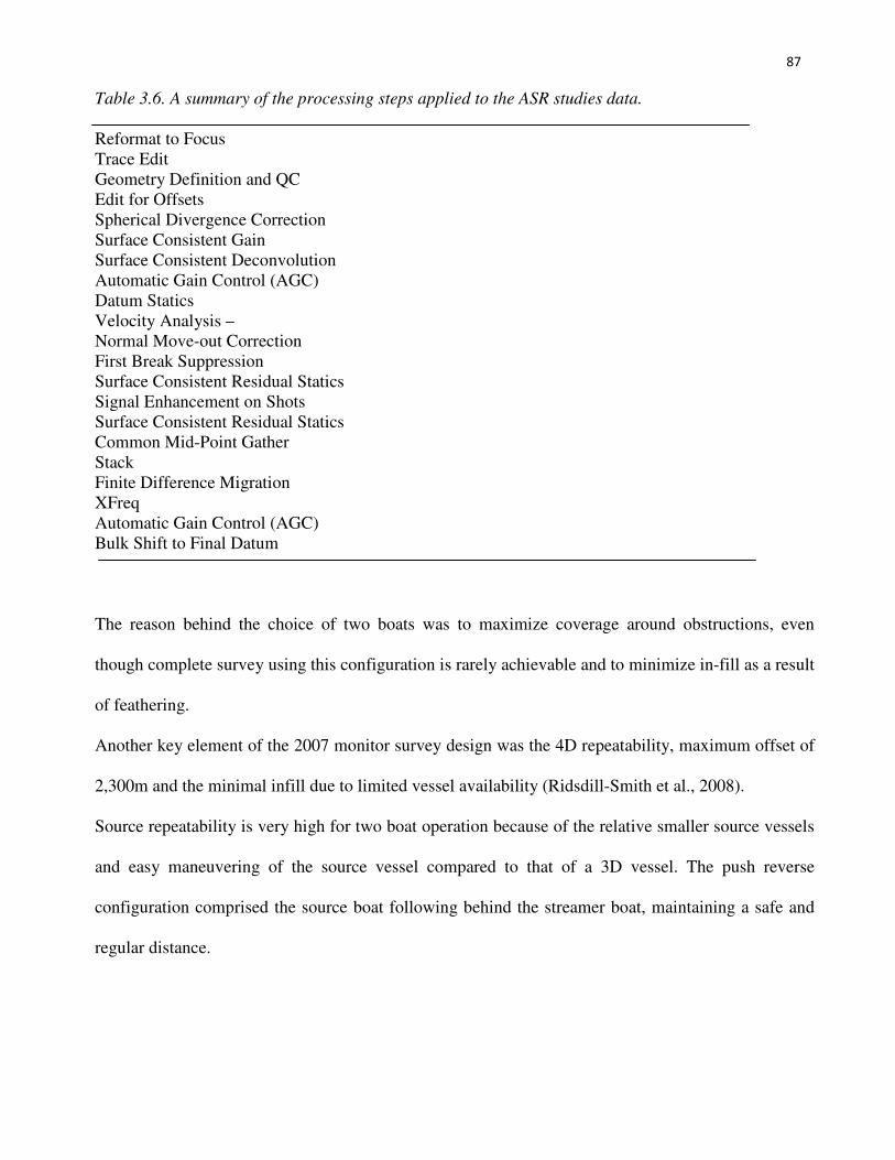
87

Table 3.6. A summary of the processing steps applied to the ASR studies data.

Reformat to Focus

Trace Edit

Geometry Definition and QC

Edit for Offsets

Spherical Divergence Correction

Surface Consistent Gain

Surface Consistent Deconvolution

Automatic Gain Control (AGC)

Datum Statics

Velocity Analysis –

Normal Move-out Correction

First Break Suppression

Surface Consistent Residual Statics

Signal Enhancement on Shots

Surface Consistent Residual Statics

Common Mid-Point Gather

Stack

Finite Difference Migration

XFreq

Automatic Gain Control (AGC)

Bulk Shift to Final Datum

The reason behind the choice of two boats was to maximize coverage around obstructions, even

though complete survey using this configuration is rarely achievable and to minimize in-fill as a result

of feathering.

Another key element of the 2007 monitor survey design was the 4D repeatability, maximum offset of

2,300m and the minimal infill due to limited vessel availability (Ridsdill-Smith et al., 2008).

Source repeatability is very high for two boat operation because of the relative smaller source vessels

and easy maneuvering of the source vessel compared to that of a 3D vessel. The push reverse

configuration comprised the source boat following behind the streamer boat, maintaining a safe and

regular distance.

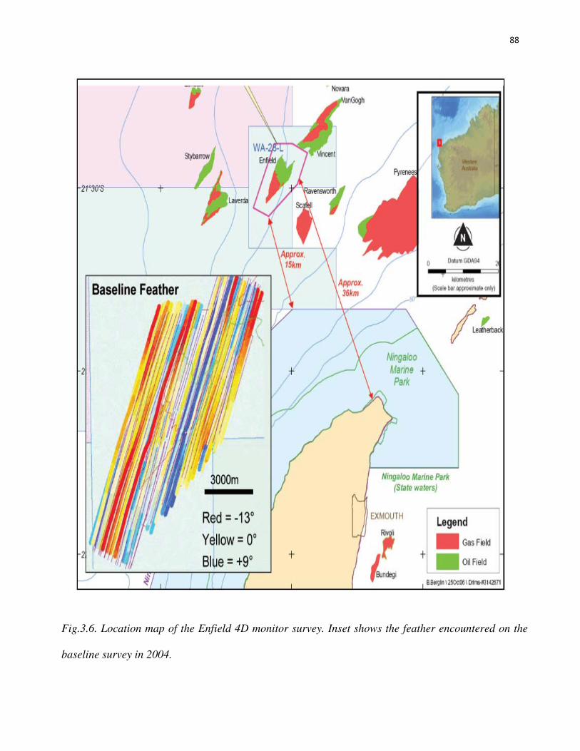
88

Fig.3.6. Location map of the Enfield 4D monitor survey. Inset shows the feather encountered on the

baseline survey in 2004.

89

Data acquisition

The Enfield monitor survey followed the same acquisition parameters as the previously conducted

baseline survey. It followed the same baseline shot-point interval of 18.7

5m (flip-flop), gun separation of 50m and the streamer vessel was steered to match the baseline

receiver positions at a target offset of 1900m.

At the time of the monitor survey, Woodside had only a 4-streamer vessel which couldn’t replicate

the 6-streamer baseline coverage and so, an 8-streamer coverage was used.

3.10. Case 9: 3D Interpretation of the Espoir Field Area, Offshore Ivory Coast.

The Espoir field was discovered in 1980 by a joint venture comprising Philips Petroleum Co., AGIP,

SEDCO Energy and PETROCI. It is located at about 13km (8 mi) offshore Ivory Coast. From

October 1981 to February 1982, GSI carried out a 3D seismic survey which covered 7,700 kilometer

line of data. The area is located on the edge of the continental shelf and extends into deep waters

(fig.3.7).

Before the 3D survey, a previous survey had been carried out on the same area which led to the

drilling of the discovery well A-1X, which was drilled in approximately 515m of water to test a

structural high at the Albian unconformity level. Hydrocarbon was struck.

An appraisal well, A-2X, was also drilled to confirm the presence of hydrocarbon-bearing and

reservoir-quality sands beneath the unconformity surface in the area. A similar exploration in the

adjacent B1 block also revealed interesting features and thus, the need to perform an extensive 3D

survey operation on the area became necessary. The aim of the 3D survey was to obtain a detailed

mapping of the Albian structure.

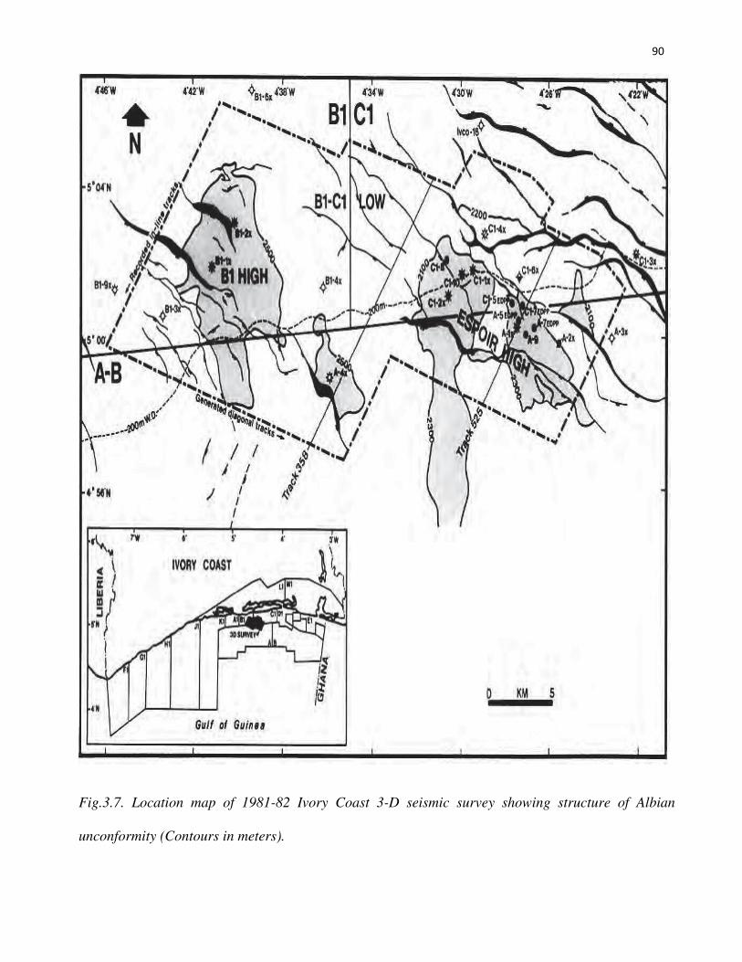
90

Fig.3.7. Location map of 1981-82 Ivory Coast 3-D seismic survey showing structure of Albian

unconformity (Contours in meters).

91

Data acquisition

The seismic program consisted of 7,700 km line of data containing 525 northeast-southwest-trending

lines acquired in a single survey area located on the edge of the continental shelf and extending into

deep water. Data was recorded using a 2,400m cable and GSI’s 4,000-cu inch air gun source.

3.11. Case 10: Structural and stratigraphic mapping of Emi field, offshore Niger Delta, Nigeria.

Emi field is located in the offshore depobelt (temporally and genetically related families of growth

fault trends or macro-structures) of the Niger Delta and covers an area of 58.24 (fig. 3.8). The

Niger Delta basin is dated as Cenozoic in age and is situated on continental margin of the Gulf of

Guinea in equatorial West Africa. The northern edge of the delta is demarcated by the Cretaceous

Abakaliki anticline, extending further to the southeast as the Afikpo syncline and Calabar flank. To

the northeast of the Niger Delta, is the structurally defined Benue hinge line, while the sediments of

Okitipupa ridge mark the western boundary of the delta (Ugwu and Ezeh., 2012).

The Niger Delta clastic wedge which spans to about 75,000 in southern Nigeria and the gulf of

Guinea, offshore Nigeria, contains reserves of about 34 billion barrels of oil and 93 trillion cubic feet

of gas and results to the 12th

largest accumulation of hydrocarbon reserve the world over (Tuttle et al.,

1999).

The deposits of the Niger Delta is divided into three large-scale lithostratigraphic units; the basal

palocene to recent pro-delta facies of the Akata region, the Eocene of recent paralic facies of the

Agbada region and the Oligocene-recent fluvial facies of the Benin formation (Evamy et al., 1978;

Short and Stauble, 1967; Whiteman, 1982)

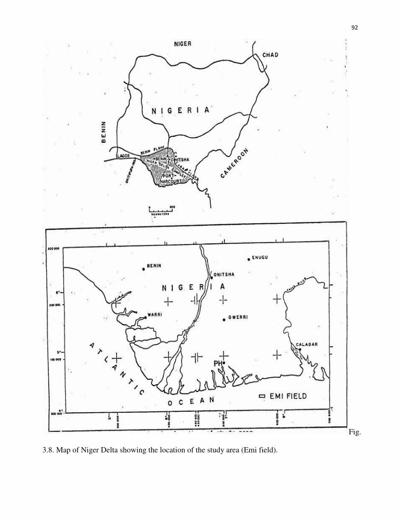
92

Fig.

3.8. Map of Niger Delta showing the location of the study area (Emi field).

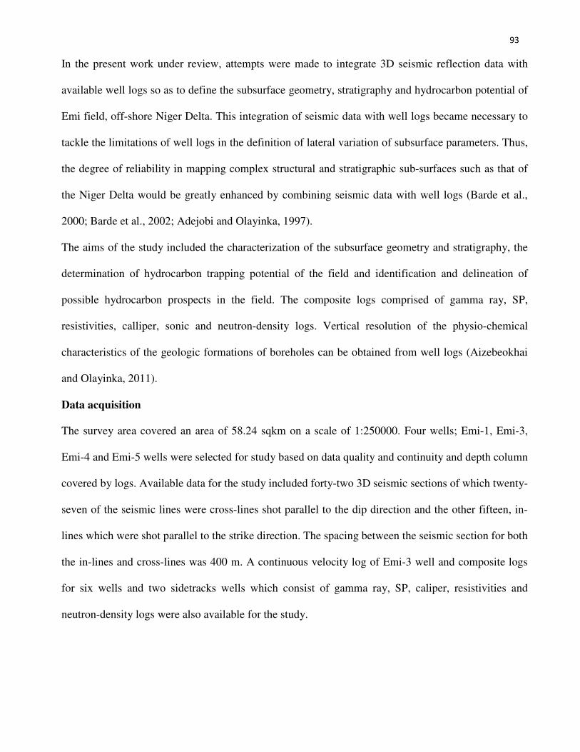
93

In the present work under review, attempts were made to integrate 3D seismic reflection data with

available well logs so as to define the subsurface geometry, stratigraphy and hydrocarbon potential of

Emi field, off-shore Niger Delta. This integration of seismic data with well logs became necessary to

tackle the limitations of well logs in the definition of lateral variation of subsurface parameters. Thus,

the degree of reliability in mapping complex structural and stratigraphic sub-surfaces such as that of

the Niger Delta would be greatly enhanced by combining seismic data with well logs (Barde et al.,

2000; Barde et al., 2002; Adejobi and Olayinka, 1997).

The aims of the study included the characterization of the subsurface geometry and stratigraphy, the

determination of hydrocarbon trapping potential of the field and identification and delineation of

possible hydrocarbon prospects in the field. The composite logs comprised of gamma ray, SP,

resistivities, calliper, sonic and neutron-density logs. Vertical resolution of the physio-chemical

characteristics of the geologic formations of boreholes can be obtained from well logs (Aizebeokhai

and Olayinka, 2011).

Data acquisition

The survey area covered an area of 58.24 sqkm on a scale of 1:250000. Four wells; Emi-1, Emi-3,

Emi-4 and Emi-5 wells were selected for study based on data quality and continuity and depth column

covered by logs. Available data for the study included forty-two 3D seismic sections of which twenty-

seven of the seismic lines were cross-lines shot parallel to the dip direction and the other fifteen, in-

lines which were shot parallel to the strike direction. The spacing between the seismic section for both

the in-lines and cross-lines was 400 m. A continuous velocity log of Emi-3 well and composite logs

for six wells and two sidetracks wells which consist of gamma ray, SP, caliper, resistivities and

neutron-density logs were also available for the study.

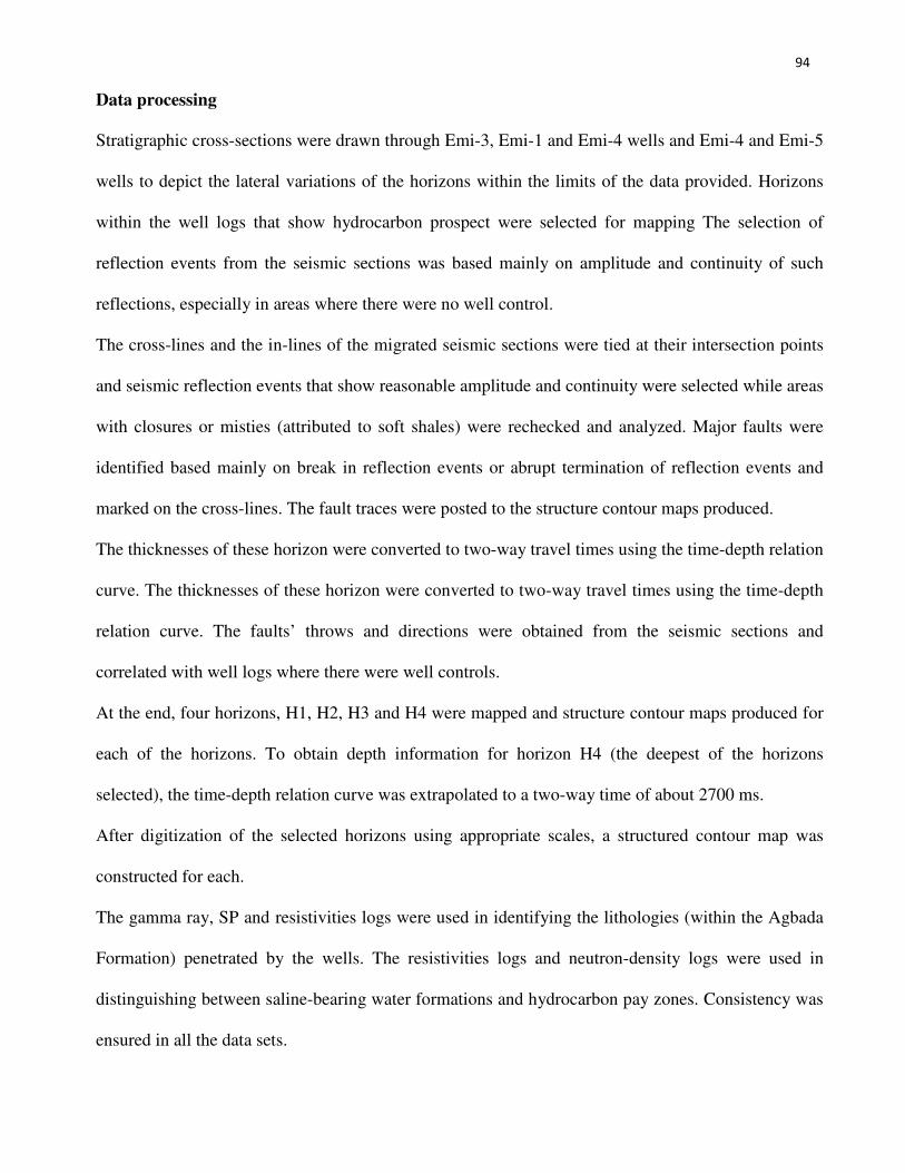
94

Data processing

Stratigraphic cross-sections were drawn through Emi-3, Emi-1 and Emi-4 wells and Emi-4 and Emi-5

wells to depict the lateral variations of the horizons within the limits of the data provided. Horizons

within the well logs that show hydrocarbon prospect were selected for mapping The selection of

reflection events from the seismic sections was based mainly on amplitude and continuity of such

reflections, especially in areas where there were no well control.

The cross-lines and the in-lines of the migrated seismic sections were tied at their intersection points

and seismic reflection events that show reasonable amplitude and continuity were selected while areas

with closures or misties (attributed to soft shales) were rechecked and analyzed. Major faults were

identified based mainly on break in reflection events or abrupt termination of reflection events and

marked on the cross-lines. The fault traces were posted to the structure contour maps produced.

The thicknesses of these horizon were converted to two-way travel times using the time-depth relation

curve. The thicknesses of these horizon were converted to two-way travel times using the time-depth

relation curve. The faults’ throws and directions were obtained from the seismic sections and

correlated with well logs where there were well controls.

At the end, four horizons, H1, H2, H3 and H4 were mapped and structure contour maps produced for

each of the horizons. To obtain depth information for horizon H4 (the deepest of the horizons

selected), the time-depth relation curve was extrapolated to a two-way time of about 2700 ms.

After digitization of the selected horizons using appropriate scales, a structured contour map was

constructed for each.

The gamma ray, SP and resistivities logs were used in identifying the lithologies (within the Agbada

Formation) penetrated by the wells. The resistivities logs and neutron-density logs were used in

distinguishing between saline-bearing water formations and hydrocarbon pay zones. Consistency was

ensured in all the data sets.

95

CHAPTER FOUR

RESULT DISCUSSION

4.1. Results of Case 1

The data acquired as described in the previous chapter, each underwent different acquisition and

processing operations and as such, one would expect different results. This chapter intends to

compare the results obtained in the cases discussed in chapter three.

For profile 1, a constant velocity analysis shows that the best stacking velocity for this profile is in the

order of 11,000m/s. Bearing in mind that the stacking velocities for dipping events depend on the dip

of the reflector, imaging clearly, all dip directions in one location tends to be a difficult task. To

correct for this, a DMO correction was applied to the data set. After which, reflections with

conflicting dips were successfully imaged with stacking velocities in the order of 6,500m/s.

A brute stacked section of the data (fig. 4.1a) before and (fig. 4.1b) after the application of refraction

and residual statics correction as well as time and space-variants band-pass filters can be seen in

figure 4.1. The band-pass filter enabled clearer coherent reflections as seen in the comparison of both

displayed sections. Strong reflectivity can be seen after 2s in (b), dipping northwards between CDPs

1,000 and 1,800 and series of sub-horizontal reflections are imaged between CDPs 90 and 800,

starting at 2.5s. Several clear reflections can be observed within the region but a very interesting

feature is an apparent south dipping that appears to approach the survey very close to the Kristineberg

mine.

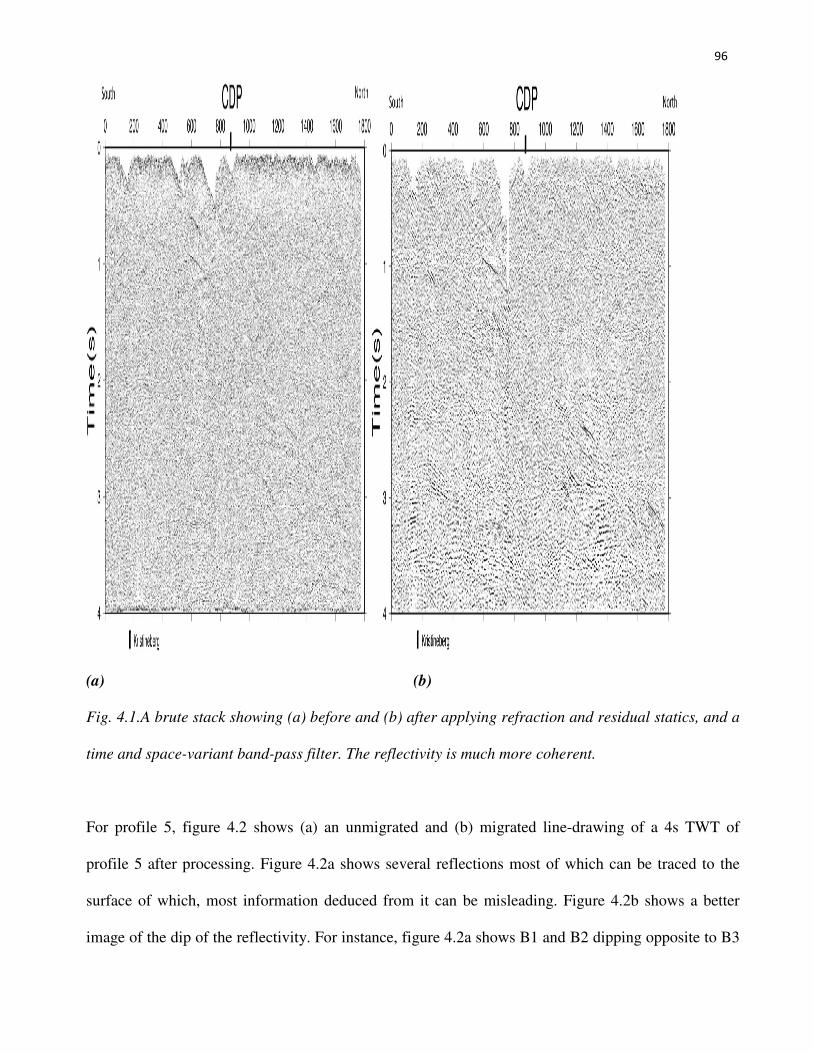
96

(a) (b)

Fig. 4.1.A brute stack showing (a) before and (b) after applying refraction and residual statics, and a

time and space-variant band-pass filter. The reflectivity is much more coherent.

For profile 5, figure 4.2 shows (a) an unmigrated and (b) migrated line-drawing of a 4s TWT of

profile 5 after processing. Figure 4.2a shows several reflections most of which can be traced to the

surface of which, most information deduced from it can be misleading. Figure 4.2b shows a better

image of the dip of the reflectivity. For instance, figure 4.2a shows B1 and B2 dipping opposite to B3

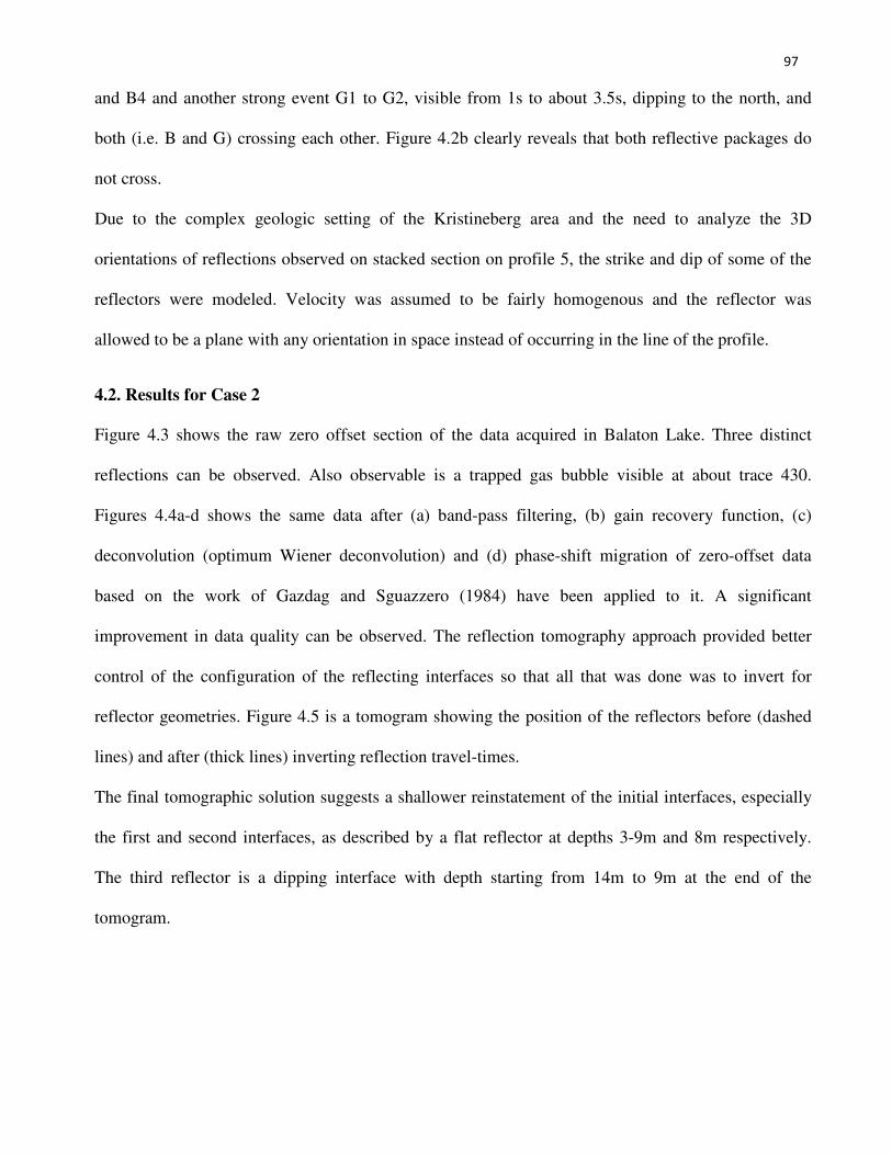
97

and B4 and another strong event G1 to G2, visible from 1s to about 3.5s, dipping to the north, and

both (i.e. B and G) crossing each other. Figure 4.2b clearly reveals that both reflective packages do

not cross.

Due to the complex geologic setting of the Kristineberg area and the need to analyze the 3D

orientations of reflections observed on stacked section on profile 5, the strike and dip of some of the

reflectors were modeled. Velocity was assumed to be fairly homogenous and the reflector was

allowed to be a plane with any orientation in space instead of occurring in the line of the profile.

4.2. Results for Case 2

Figure 4.3 shows the raw zero offset section of the data acquired in Balaton Lake. Three distinct

reflections can be observed. Also observable is a trapped gas bubble visible at about trace 430.

Figures 4.4a-d shows the same data after (a) band-pass filtering, (b) gain recovery function, (c)

deconvolution (optimum Wiener deconvolution) and (d) phase-shift migration of zero-offset data

based on the work of Gazdag and Sguazzero (1984) have been applied to it. A significant

improvement in data quality can be observed. The reflection tomography approach provided better

control of the configuration of the reflecting interfaces so that all that was done was to invert for

reflector geometries. Figure 4.5 is a tomogram showing the position of the reflectors before (dashed

lines) and after (thick lines) inverting reflection travel-times.

The final tomographic solution suggests a shallower reinstatement of the initial interfaces, especially

the first and second interfaces, as described by a flat reflector at depths 3-9m and 8m respectively.

The third reflector is a dipping interface with depth starting from 14m to 9m at the end of the

tomogram.

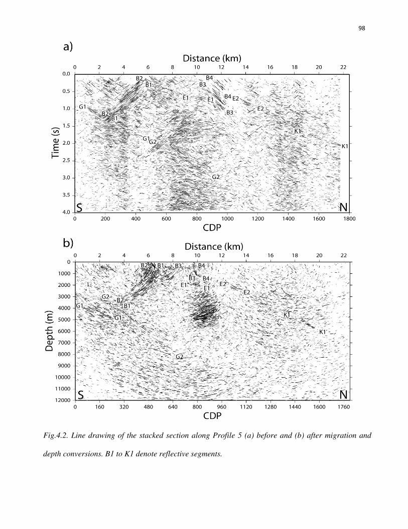
98

Fig.4.2. Line drawing of the stacked section along Profile 5 (a) before and (b) after migration and

depth conversions. B1 to K1 denote reflective segments.

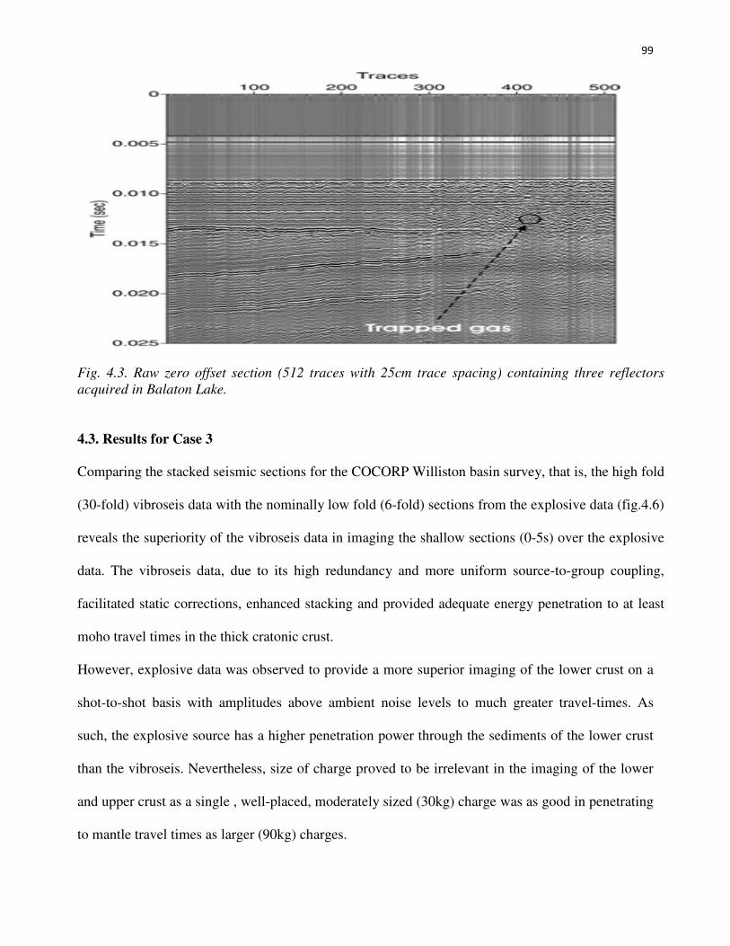
99

Fig. 4.3. Raw zero offset section (512 traces with 25cm trace spacing) containing three reflectors

acquired in Balaton Lake.


Comparing the stacked seismic sections for the COCORP Williston basin survey, that is, the high fold

(30-fold) vibroseis data with the nominally low fold (6-fold) sections from the explosive data (fig.4.6)

reveals the superiority of the vibroseis data in imaging the shallow sections (0-5s) over the explosive

data. The vibroseis data, due to its high redundancy and more uniform source-to-group coupling,

facilitated static corrections, enhanced stacking and provided adequate energy penetration to at least

moho travel times in the thick cratonic crust.

However, explosive data was observed to provide a more superior imaging of the lower crust on a

shot-to-shot basis with amplitudes above ambient noise levels to much greater travel-times. As

such, the explosive source has a higher penetration power through the sediments of the lower crust

than the vibroseis. Nevertheless, size of charge proved to be irrelevant in the imaging of the lower

and upper crust as a single , well-placed, moderately sized (30kg) charge was as good in penetrating

to mantle travel times as larger (90kg) charges.

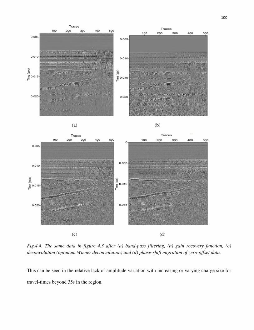
100

(a) (b)

(c) (d)

Fig.4.4. The same data in figure 4.3 after (a) band-pass filtering, (b) gain recovery function, (c)

deconvolution (optimum Wiener deconvolution) and (d) phase-shift migration of zero-offset data.

This can be seen in the relative lack of amplitude variation with increasing or varying charge size for

travel-times beyond 35s in the region.

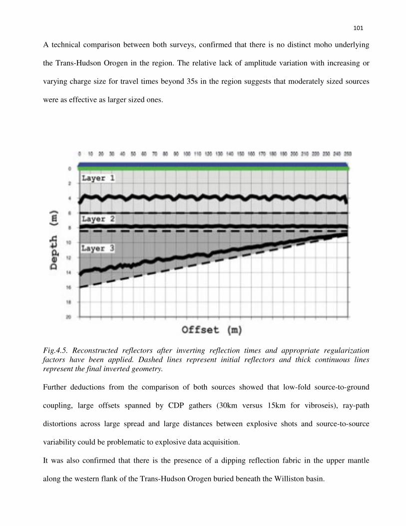
101

A technical comparison between both surveys, confirmed that there is no distinct moho underlying

the Trans-Hudson Orogen in the region. The relative lack of amplitude variation with increasing or

varying charge size for travel times beyond 35s in the region suggests that moderately sized sources

were as effective as larger sized ones.

Fig.4.5. Reconstructed reflectors after inverting reflection times and appropriate regularization

factors have been applied. Dashed lines represent initial reflectors and thick continuous lines

represent the final inverted geometry.

Further deductions from the comparison of both sources showed that low-fold source-to-ground

coupling, large offsets spanned by CDP gathers (30km versus 15km for vibroseis), ray-path

distortions across large spread and large distances between explosive shots and source-to-source

variability could be problematic to explosive data acquisition.

It was also confirmed that there is the presence of a dipping reflection fabric in the upper mantle

along the western flank of the Trans-Hudson Orogen buried beneath the Williston basin.

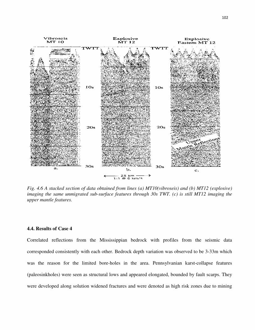
102

Fig. 4.6 A stacked section of data obtained from lines (a) MT10(vibroseis) and (b) MT12 (explosive)

imaging the same unmigrated sub-surface features through 30s TWT. (c) is still MT12 imaging the

upper mantle features.


Correlated reflections from the Mississippian bedrock with profiles from the seismic data

corresponded consistently with each other. Bedrock depth variation was observed to be 3-33m which

was the reason for the limited bore-holes in the area. Pennsylvanian karst-collapse features

(paleosinkholes) were seen as structural lows and appeared elongated, bounded by fault scarps. They

were developed along solution widened fractures and were denoted as high risk zones due to mining

103

activities performed on the area. Low risk areas are those areas that were structurally elevated and

were less likely to be mining sites.

The GPS profiles crossed undisturbed clay-rich residual soil overlain by a thin veneer of chat. The

chat/soil contact was easily identified and correlated across the GPR profile. Those profiles imaged

in-fill mine access shafts. The result suggested that materials had been displaced possibly by a

bulldozer to fill local drive way surfaces, as much of the chat had been illegally gathered away. The

chat/soil interface is regular in character and continuous except where the GPR profile crosses the

mine access or ventilation shaft.


The USGS at the time, lacked software packages to interpolate automatically and smoothen all the

average velocity analyses generated in the ANWR seismic re-processing into a 3D model. If it

weren’t so, an improved second order anomaly in the velocity model would have been obtained.

However, only one 3D velocity model for the top of the pre-Mississippian meta-sedimentary rock

horizon could be obtained in the survey.

The re-processing of the seismic data derived in 1984/85 for the 1998 assessment in 1996/97 was able

to improve significantly the temporal resolution of the data over the area. Consistent wavelets were

generated through the wavelet processing which merged satisfactorily to improve data quality. By

merging appropriate lines also, the edge effect of the migration and velocity field was reduced. This

also improved image quality of the data.


The results obtained showed the same basic reflection as in the initial survey although the image

clarity differed as a result of the different sources used, different ground conditions and differences in

depth to A/E. The very dry ground in the latter survey resulted in the less effective power of both the

104

hammer and Buffalo gun sources at higher frequencies when compared to the former, thus, reducing

energy seen at depth and consequently, their reflection amplitude.

Data from both surveys were observed to tie well in areas where the depth to A/E is similar and show

poor events in areas where the depth to A/E is at 50% of its depth at the other side.

The very shallow parts of the data was degraded by noise generated at the shot-point and so produced

fewer usable traces. Though degraded in quality, the obtained sections reproduced the desired cross-

sectional information which includes the A/E interface, intra-Eagle Ford reflection, the base of the

Eagle Ford and the strong deeper reflections from below the Eagle Ford.

The processing operation was able to remove noise, especially surface waves, increase data resolution

and adjust for topographic and irregular weathering-related time shifts. It was also able to combine

separate results which increased signal levels.

The interpretation was based on the continuity of all cross-sectional information and how they tie to

sonic logs and shallow bore-hole data along the line. By following the continuity of a specific

reflection, the dip changes and/or fault offset of that bed can be determined.

The data was structurally interpreted to have significant disruptions in a few zones along the line.

Three zones of possible faulting were interpreted. These zones were generally grabens or normal

faults with displacements of about 20ft. Those fault features were fairly distinct and separate. There

was no clear tie between faults at depth with shallower faults which cut the Austin.


An obvious improvement was observed on the stacked section, the migrated section and the stacks on

which the enhanced frequency technique was applied, with the latest showing better reflection

continuity and resolution. The migration process significantly reduced scattering of reflections.

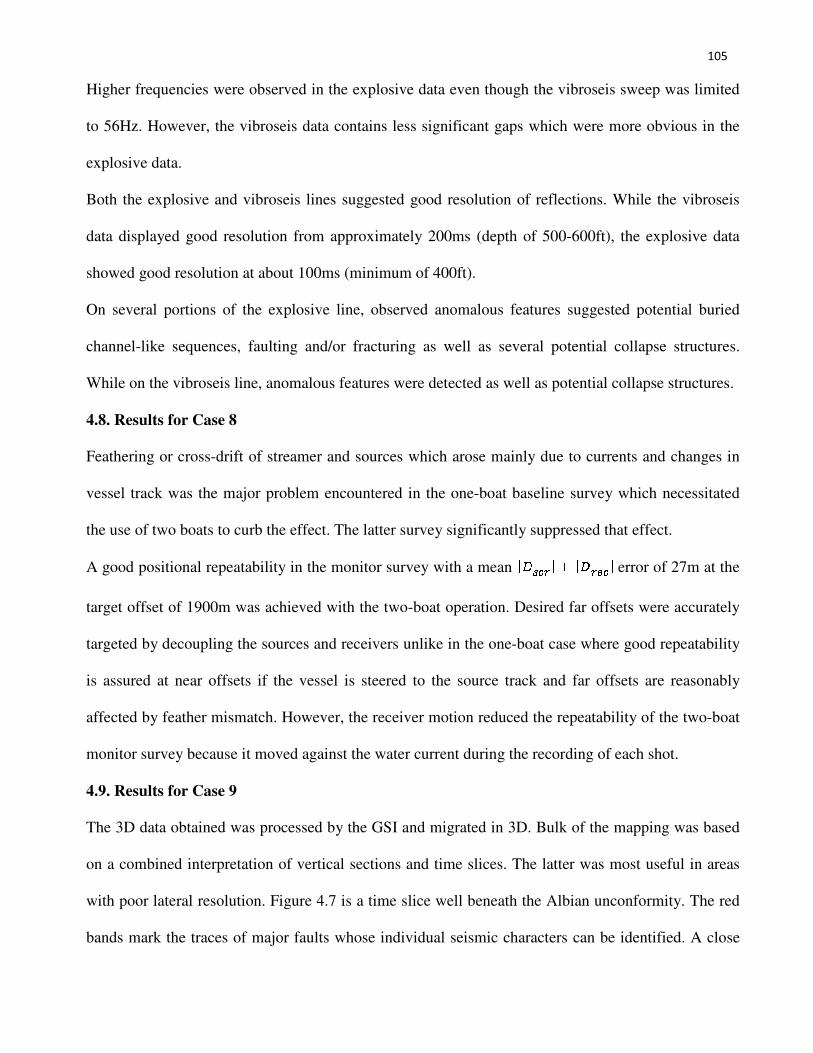
105

Higher frequencies were observed in the explosive data even though the vibroseis sweep was limited

to 56Hz. However, the vibroseis data contains less significant gaps which were more obvious in the

explosive data.

Both the explosive and vibroseis lines suggested good resolution of reflections. While the vibroseis

data displayed good resolution from approximately 200ms (depth of 500-600ft), the explosive data

showed good resolution at about 100ms (minimum of 400ft).

On several portions of the explosive line, observed anomalous features suggested potential buried

channel-like sequences, faulting and/or fracturing as well as several potential collapse structures.

While on the vibroseis line, anomalous features were detected as well as potential collapse structures.


Feathering or cross-drift of streamer and sources which arose mainly due to currents and changes in

vessel track was the major problem encountered in the one-boat baseline survey which necessitated

the use of two boats to curb the effect. The latter survey significantly suppressed that effect.

A good positional repeatability in the monitor survey with a mean error of 27m at the

target offset of 1900m was achieved with the two-boat operation. Desired far offsets were accurately

targeted by decoupling the sources and receivers unlike in the one-boat case where good repeatability

is assured at near offsets if the vessel is steered to the source track and far offsets are reasonably

affected by feather mismatch. However, the receiver motion reduced the repeatability of the two-boat

monitor survey because it moved against the water current during the recording of each shot.


The 3D data obtained was processed by the GSI and migrated in 3D. Bulk of the mapping was based

on a combined interpretation of vertical sections and time slices. The latter was most useful in areas

with poor lateral resolution. Figure 4.7 is a time slice well beneath the Albian unconformity. The red

bands mark the traces of major faults whose individual seismic characters can be identified. A close

106

look at the top part of the figure however, indicates a zone of poor data quality resulting to fault traces

not being adequately mapped. In such cases, closely spaced (60m) vertical sections were used to

define fault traces. They were also used to correlate weak or complex reflections and to map smaller

depositional units. An improved velocity derived from the closely spaced velocity analysis was used

to prepare depth maps at the reservoir level.

Data obtained from the 3D survey when compared to the previous 2D survey done on the same area,

aided interpretation and mapping by providing sharper definition of structural features, showing more

reliable correlation of horizons and fault traces between closely spaced tracks. It also aided in the

preparation of detailed time contour maps from time-slice sections and an improved velocity depth

model for depth conversion. In defining structural features, a comparison can be made of a migrated

section of the 2D and 3D data. Figure 4.8 shows the two versions of line 358 which crosses a feature

near A-4X. Although at about time 2.7s, an evidence of anomaly can be seen at the centre of the

figure but the feature itself is not clear. On the same data after 3D migration (right), a more improved

detail is observed. It shows a steeply-dipping intra-Albian reflection cutting through a flat spot which

is close to a fluid contact defined in well A-4X.

4.10. Results of case 10

The stratigraphic cross-section through Emi-4 and Emi-5 wells tended to be more horizontal and

parallel to one another than those of the cross-section through Emi-4, Emi-1 and Emi-3. This is

because Emi-4 and Emi-5 are more or less in the same strike direction compared to Emi-4, Emi-1 and

Emi-3.

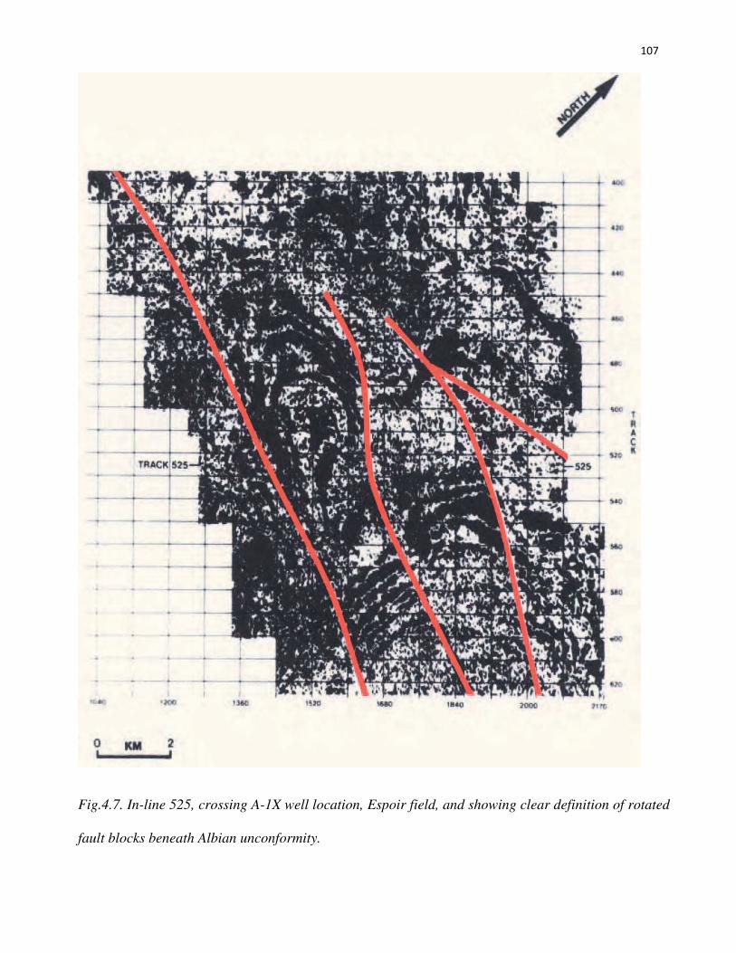
107

Fig.4.7. In-line 525, crossing A-1X well location, Espoir field, and showing clear definition of rotated

fault blocks beneath Albian unconformity.

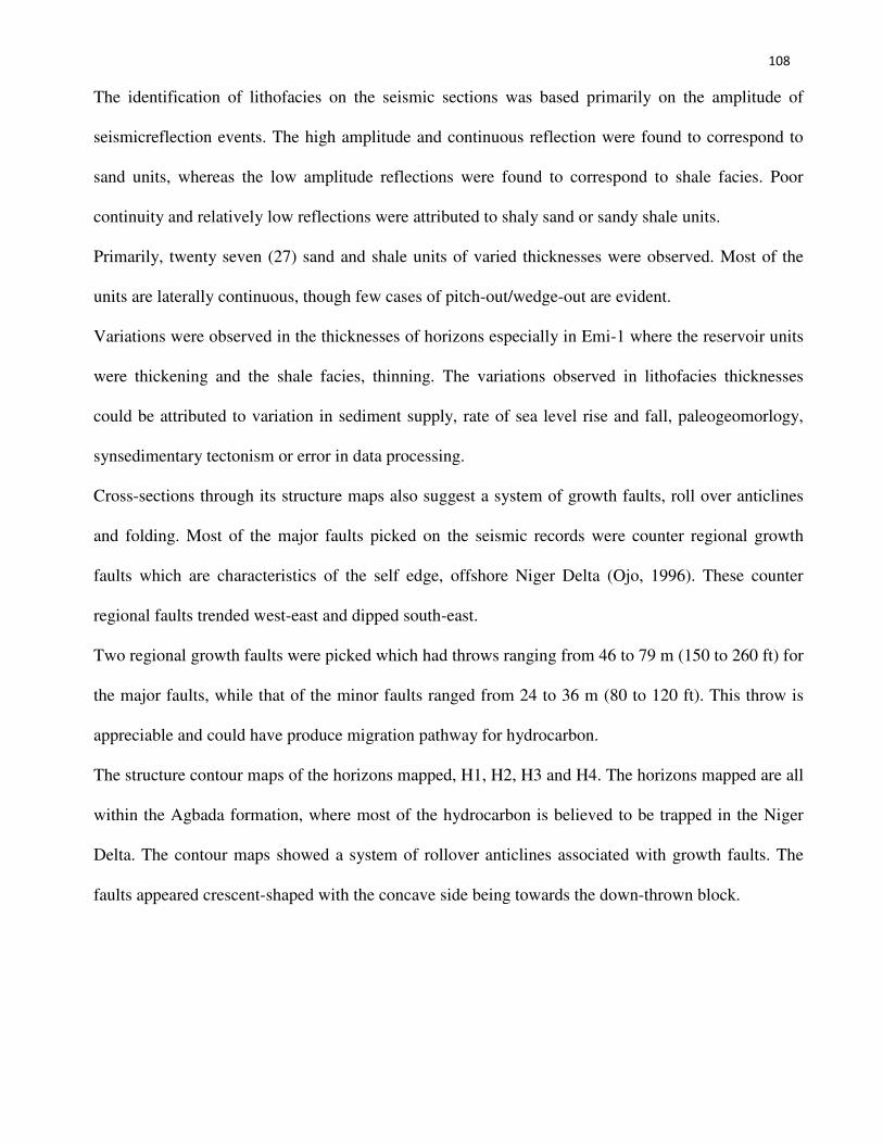
108

The identification of lithofacies on the seismic sections was based primarily on the amplitude of

seismicreflection events. The high amplitude and continuous reflection were found to correspond to

sand units, whereas the low amplitude reflections were found to correspond to shale facies. Poor

continuity and relatively low reflections were attributed to shaly sand or sandy shale units.

Primarily, twenty seven (27) sand and shale units of varied thicknesses were observed. Most of the

units are laterally continuous, though few cases of pitch-out/wedge-out are evident.

Variations were observed in the thicknesses of horizons especially in Emi-1 where the reservoir units

were thickening and the shale facies, thinning. The variations observed in lithofacies thicknesses

could be attributed to variation in sediment supply, rate of sea level rise and fall, paleogeomorlogy,

synsedimentary tectonism or error in data processing.

Cross-sections through its structure maps also suggest a system of growth faults, roll over anticlines

and folding. Most of the major faults picked on the seismic records were counter regional growth

faults which are characteristics of the self edge, offshore Niger Delta (Ojo, 1996). These counter

regional faults trended west-east and dipped south-east.

Two regional growth faults were picked which had throws ranging from 46 to 79 m (150 to 260 ft) for

the major faults, while that of the minor faults ranged from 24 to 36 m (80 to 120 ft). This throw is

appreciable and could have produce migration pathway for hydrocarbon.

The structure contour maps of the horizons mapped, H1, H2, H3 and H4. The horizons mapped are all

within the Agbada formation, where most of the hydrocarbon is believed to be trapped in the Niger

Delta. The contour maps showed a system of rollover anticlines associated with growth faults. The

faults appeared crescent-shaped with the concave side being towards the down-thrown block.

109

Fig.4.8. Comparison of 2-D migration and 3-Dmigration sections across structure drilled by well A-

4X showing improved definition of erosional high on Albian unconformity and fluid contact (flat

spot).

Faulted and folded anticlinal closures were common structures observed in all horizons. These

closures serve as good traps for hydrocarbon and are therefore possible hydrocarbon prospects. Apart

from delineating the structural traps, other stratigraphic features such as pinch-outs, unconformities,

sand lenses and channels were also suspected.

110

CHAPTER FIVE

DISCUSSIONS AND CONCLUSION

5.1. Discussion and conclusions

The successful interpretation of a seismic data, be it 2-D/3-D or land/marine, depends on proper

survey design, acquisition and processing, guarding against pit-falls and optimal utilization of

available technology. The cases reviewed in this work each had different objectives and as a result,

underwent different processing approaches.

This review has been able to demonstrate the usefulness and limitations of certain approaches to

seismic operations. It has also been able to establish the fact that seismic reflection method remains a

very vital and indispensable tool in the analysis and structural mapping of the sub-surface.

Today, more and more advancements have been recorded in the exploration industry, such

advancements include 4-D seismic survey (time-lapse), multi-streamer and multi vessel survey for

marine operations and enhanced oil recovery (EOR) which are current trends in seismic survey and

are gaining popularity in the area of reservoir evaluation, prediction of future productions and

hydrocarbon recovery. There is today an increasing interest in the other forms of energy such as S-

waves that arrive at the surface spread other than P-waves which are only part of the wave field.

These other forms of energy may be mode converted from a down-going impulsive source or may

arise from a shear wave source capable of outputting both compressional and shear waves chances

are that more developments will be achieved having better of these waves.

Technological advancements which have also richly enhanced interactive software allow users to

iterate parameters and view effects on screen almost immediately in animated form. Such software

111

have been integrated with measurements, analyses, interpretation and reservoir properties to help the

interpreters work better.

The reviewed cases have been able to demonstrate that it is possible to determine the strike and dip of

reflectors using the crooked line geometry.

It was also able to prove that the tomographic approach is capable of providing depth models even in

the absence of bore-hole control and velocity analysis. On the other hand, the tomographic approach

was not able to detect and define the biogenic gas bubbles present in the raw seismic data even though

it was able to locate the anomalous points. This was due to the relatively large wavelength used.

Another reviewed case of the Niger Delta of Nigeria was able to demonstrate that the integration of

seismic data and well logs is a useful and valid tool in structural and stratigraphic mapping and in

better definition of the subsurface geometry and hydrocarbon trapping potential.

The usefulness and limitations of vibroseis and explosive sources for deep crustal and upper mantle

exploration was also revealed in the profiling of the Williston basin. The vibroseis data produced a

more uniform source to group coupling and also a better image of the upper crust while the explosive

data, due to its high penetration ability gave a better image of the lower crust.

It also established the fact that reflection seismic survey can be used to map bedrocks and bedrock

related features such as faults and paleosinkholes and also to map boundaries of previous mine sites.

A knowledge of faults and shear zones, sinkholes etc, helped avert potential highway and/or

construction hazards and aided route planning.

The re-processing of the seismic data derived in 1984/85 for the 1998 assessment in 1996/97, was

able to improve significantly the temporal resolution of the data over the area. This goes to buttress

the improvements recorded in the industry as a result of technological advancements. Today, we have

112

even more improved software some of which include Petrel, , , ,

to mention but a few.

We also re-established the fact that data from a small source (sledge hammer) could also be used to

image the upper crust with as much clarity as that of a large source if there is proper coupling of the

source to the ground and adequate processing sequences applied.

The use of modern software and hardware in data processing as elaborated in the seismic processing

and velocity assessments in the oil and gas resource potential of the 1002 area emphasizes on better

processing operations using more modern equipment. Much emphasis was placed in the ASR regional

study case on XFreq, a modern software (at that time), which boosted amplitudes of the higher

frequency range and thus produced a more enhanced frequency content of the data.

It also shows that explosive data have higher frequency content than vibratory data and as such would

image deeper layers better.

For marine operations, multi-streamer surveys curb such limitations such as feathering which was

inherent in the reviewed one boat survey, provides a good positional repeatability and allows better

coverage of the survey area.

The superiority of 3D over 2D survey was also demonstrated in this review. The 3D survey data

brought about a better definition of pre-unconformity reflections which resulted in better mapping of

the intra-Albian horizons and better correlations across major faults. Such improved mappings aided

in the identification of additional wells.

5.2. RECOMMENDATION

In line with the conclusions reached from the reviewed seismic reflection operations, we hereby

recommend that adequate caution should be taken against pitfalls and errors especially during the

113

acquisition and processing of seismic data, since any error in either regard will be quite misleading

during interpretation.

We also recommend that acquired seismic data should be integrated with available well logs to

provide a more reliable and better definition of the sub-surface.

We were able to see that dynamite sources provided data which gave a better definition of the deeper

crust than vibroseis and other sources and as such, we recommend a well uniform source-to-ground

coupled dynamite source for deep crustal surveys and a well impacted uniform vibroseis or any other

(boomer, hammer etc) source for shallow surveys.

To curb the effect of feathering and poor positional repeatability in marine surveys, multi-streamer

vessel survey is recommended.

In seismic data acquisition and processing, we recommend the use of more modern equipment

(hardware and software).

Lastly, for a more intensive and more detailed stratigraphic and structural definition of the earth crust

be it land or marine, we recommend a 3D survey over its 2D counterpart.

114

REFERENCES

Adejobi, A. R. and Olayinka, A. I., (1997). Stratigraphy and hydrocarbon potential of the Opuama

channel complex area, western Niger delta. Nigerian Association of petroleum Explorers

(NAPE) Bull., 12: 1-10

Aizebeokhai, A. P. and Olayinka, I., (2011), Structural and stratigraphic mapping of Emi field,

offshore Niger Delta, Nigeria. Journal of Geology and Mining Research Vol. 3(2), pp. 25-38,

February 2011.

Baird, D. J., (1995). Trans Hudson Oregen structure beneath the Williston Basin results from

COCORP seismic reflection profiling: Ph.D thesis, Cornell University

Barde, J. P., Chambertain, P., Gralla, P., Harwijanto, J., Marsky, J., Schroeter, T., (2000). Explaining

a complex hydrocarbon system in the PermoTriassic of the precaspian basin by integration of

independent models. Abstracts, 62nd European Association of Geoscientists and Engineers

Conference and Technical Exhibition, 2: (P.021), P. 4

Barde, J.P., Gralla, P., Harwijanto, J., Marsky, J., (2002). Exploration at the eastern edge of the

prescapian basin impact of data integration on Upper Permian and Trasicprospectivity.

American Association Petroleum of Geologists Bulletin, 86: 399-415.

Barrett, T.J., Maclean, W.H., (2000); Chemostratigraphy, Petrography and Alteration at the

Kristineberg VMS Deposit, Skellefte District, Sweden. Unpublished report for Boliden AB

Exploration.

Bird, K. J. and Magoon, L. B., (1987); Petroleum geology of the northern part of the Arctic National

Wildlife Refuge, northeastern Alaska: US Geological summit bulletin 1778, P. 329.

Bracewell, R. N. (1965), The Fourier transform and its application: McGraw-Hill Book Co. New

York.

Brown, A. R., Grillot, L. R.,Anderton, P. W.,Haselton, T. M. andDermargne, J. F., (2004); 3D

Interpretation of the Espoir Field Area, Offshore Ivory Coast, Interpretation of Three-

Dimensional Seismic Data, Sixth Edition; AAPG Memoir 42 SEG Investigations in

115

Geophysics, No. 9; The American Association of Petroleum Geologists and the Society of

Exploration Geophysicists, Tulsa, Oklahoma, U.S.A.

Colton, P. B. and Nautiyal, A., (1996); Cascaded Dipole Filters: Extending the Limits of Seismic

Resolution, CSEG Recorder, P. 8-19.

Constain, J. K. and Coruh, C., (2004), Basic theory of exploration seismology: Elsevier press, Oxford,

U.K.

Deregowski, S. and Rocca, F., (1981); Geometrical optics and wave theory for constant–offset

sections in layered media;, Geophysical prospecting, v. 29, P. 374.

Dobrin, M. B. and Savit, C. H., (1988), Introduction to geophysical prospecting: McGraw-Hill, New

York.

Evamy B. D., Herebourne J, Kameling P, Knap W. A., Molley, F. A., Rowlands P. H., (1978).

Hydrocarbon habitat of Tertiary Niger Delta. American Association of Petroleum Geologists

Bulletin, 62: 1-39.

Gazdag, J., and Sguazzero, P., (1984); Migration of Seismic Data by Phase Shift Plus Interpolation,

Geophysics, 49 (2), 124-131.

Grant, F. S. and West, G. F., (1965), Interpretation theory in applied geophysics: McGraw-Hill, New

York.

Gray, W. C., (1979); Variable norm deconvolution: Palo Alto, CA, Stanford University Ph.D. thesis,

P. 101.

Hatton, L., Worthington, M. H. and Makin, J., (1986), Seismic data processing (Theory and

Practice): Blackwell Scientific Publications, London.

Keary, P. and Brooks, M., (1984), An Introduction to geophysical exploration: Blackwell Scientific

Publication, England.

LCT Houston, Inc. and Dobecki Earth Sciences Houston, Texas., (1990); Seismic Reflection

Investigation of C-1 To F-1 Sector of the Superconducting Super Collider (SSC) Ring West of

Waxahachie, Texas.SSC-SR- 1137, Project No. 87-888-0022,Report No. SSCGR-78,

September 1990.

116

Lee, M. W., Agena, W. F., Grow, A. J. and Miller, J. J.,(1999); The oil and Gas potential of the 1002

area, Arctic National Wildlife Refuge, Alaska, by ANWR assessment team, U. S. Geological

Survey Open File Report 98-34.

Lee, M. W., Agena, W. F. and Hutchinson, D. R., (1988); Processing of the GLIMPCE Multi-

Channel Seismic Data: US Geological Survey Open File Report 88-225, P. 46.

Lee, W. M., (1999), Processing of Single Channel Air Ad Water Gun Data for Imaging an Impact

Structure at the Chesapeake Bay, U.S. Geological Survey Bulletin 2169, U.S. Department of

the Interior.

Lowrie, W., (2007), Fundamentals of geophysics: Cambridge University press, New York.

McLamore, V.R., Anderson, D.G., and Espana, C., (1978), Crosshole testing using explosive and

mechanical energy source, in Dynamic Geotechnical Testing. ASTM STP 654: ASTM, 30-

50.

Merki, P. J., (1972). Structural geology of the Cenozoic Niger Delta: 1st Conference on African

Geology Proceedings, Ibadan University Press, pp. 635-646.

Murat, R. C., (1970). Stratigraphy and Paleogeography of the Cretaceous and Lower Tertiary in

Southern Nigerian. 1st Conference on African Geology Proceedings, Ibadan University Press,

pp. 251-266.

Nelson, K. D., Baird, D. J., Walter, J. J., Hauck, M., Brown, L. L., Oliver, J. E., Ahern, J. L., Hajnal,

Z. and Sloss, L. L., (1993); Trans Hudson Orogen and Williston Basin in Montana and North

Dakota: New COCORP deep-profiling results: Geol., 21, P. 447-450.

Ojo, A. O., (1996). Pre-drill prospect evaluation in deep water Nigeria. Nigerian Association of

Petroleum Explorers (NAPE). Bull., 11: 11-22.Ojo, A. O., (1996).

Ridsdill-Smith, T., Flynn, D. and Darling, S., (2008); Benefits of two-boat 4D acquisition, an

Australian case study; The Leading Edge, July 2008 edition, P. 940-46

Robinson, S. R. and Coruh, C., (1988), Basic exploration geophysics: John Wiley and Sons.

Sengbush, R. L., (1983), Seismic exploration methods: IHRDC, Boston.

117

Shoemaker, M. L., Anderson, N. L., Hatheway, A. W., Newton, E. T., Cardimona, S., Shaw, A. E.,

Baker, A. J., Webb, D. and Conley, J., (2000);Reflection Seismic and Ground-Penetrating

Radar Study of Previously Mined (Lead/Zinc) Ground, Joplin, Missouri Department of

Transportation Special Publication (2000).

Short K. C., Stauble A. J., (1967). Outline of Geology of the Niger delta. American Association of

Petroleum Geologists Bulletin, 51: 761-779.

Soupios, P. M. and Toth, T., (2005); Seismic Reflection Tomography: A Case Study of a Shallow Lake

in Lake Balaton. Journal of Balkan Geophysical Society, vol. 8, no.1, February, 2005, p. 20-

27

Soupios, P.M., Papazachos, Tsokas, G.N., Vafidis, A., (2004), Nonlinear Simultaneous

Determination of Reflector Geometry and 3-D Velocity Structure, in review in Geophysical

Prospecting.

Steer, D. N., Brown, L. D., Knapp, J. H. and Baird, D. J., (1996); Comparison of Explosive and

Vibroseis Source Energy Penetration During COCORP’S Deep Seismic Reflection Profiling

in the Williston Basin. GEOPHYSICS, Vol. 61, NO. 1 (January-February 1996); P. 211-221

Telford, M. W., Geldart, L. P. and Sheriff, R. E., (1990), Applied Geophysics (Second Edition):

Cambridge University Press, New York.

Tryggvason, A., Malehmir, A., Rodriguez, J., Juhlin, C., Weihed, P. and Palm, H. (2003); Seismic

reflection studies in the Skellefte Ore District, Northern Sweden – towards a 3-D geological

model, Annual Report 1, 2003-2004

Tuttle, M. L. W., Charpentier, R. R. and Brownfield, M. E.,(1999), The Niger delta petroleum system:

Niger delta province, Nigeria, Cameroon, and Equatorial Guinea, Africa: USGS Open-file

report 99-50-H.

Ugwu, G. Z. and Ezeh, C. C., (2012), Structural and stratigraphic mapping of Emi field, offshore

Niger Delta, Nigeria. International Research Journal of Geology and Mining (IRJGM) (2276-

6618) Vol. 2(7) pp. 199-204, September 2012.

Weihed, P., Bergman, J., Bergström, U., (2001). Metallogeny and tectonic evolution of the Early

Proterozoic Skellefte district, northern Sweden. Precambrian Research 58, 143-167.

118

Whiteman, A. J., (1982). Nigeria: Its Petroleum Geology, Resources and Potentials. Graham and

Trotham, London, 2, 306-361.

Yilmaz, O., (1987), Seismic data processing: Society of exploration geophysics, Tulso Okla.

Documents

REVIEW OF SEISMIC REFLECTION - unn.edu.ng Abraham.pdf · Migration 36 ... GENERAL INTRODUCTION 1.1. Introduction Seismic reflection method is the most commonly used geophysical technique