C.1 A Sample of Data

C.2 An Econometric Model

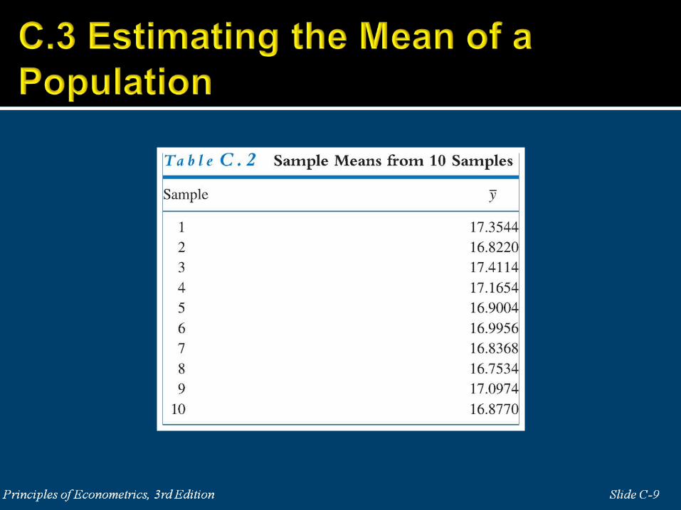
C.3 Estimating the Mean of a Population

C.4 Estimating the Population Variance and Other Moments

C.5 Interval Estimation

C.6 Hypothesis Tests About a Population Mean

C.7 Some Other Useful Tests

C.8 Introduction to Maximum Likelihood Estimation

C.9 Algebraic Supplements

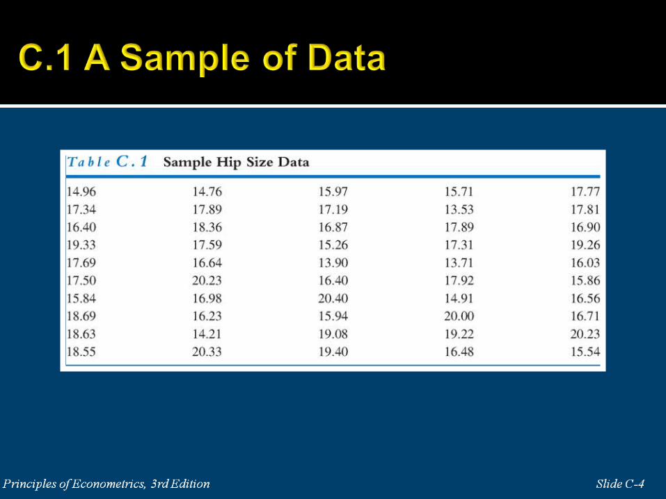
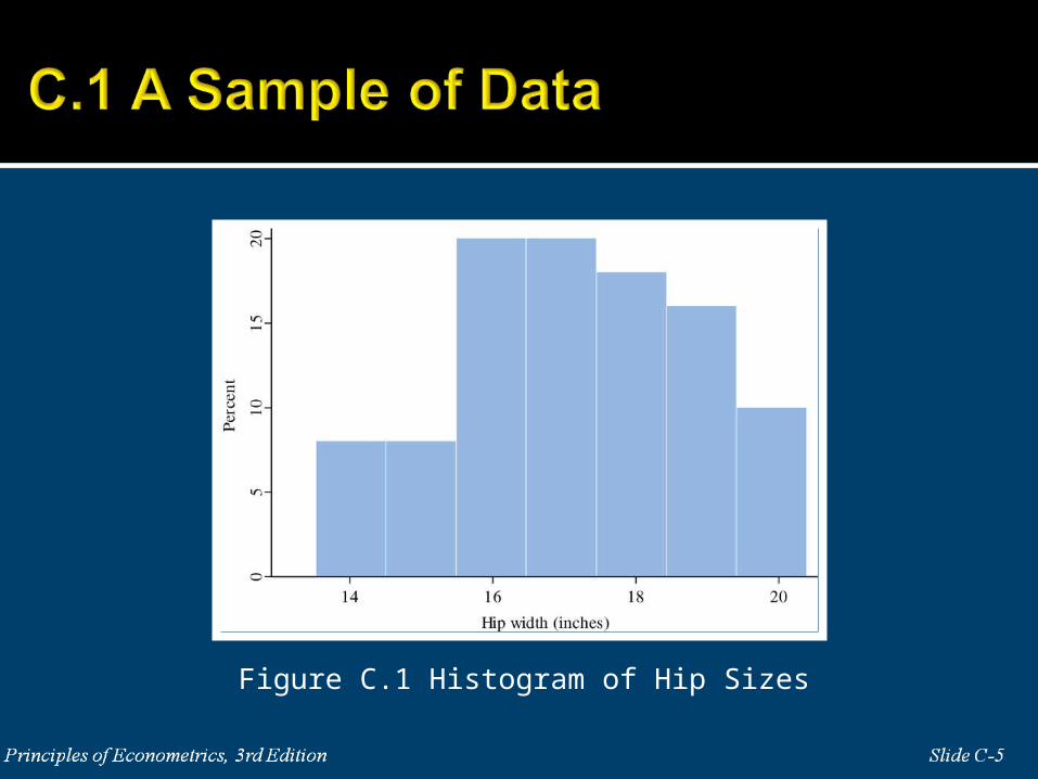
Figure C.1 Histogram of Hip Sizes

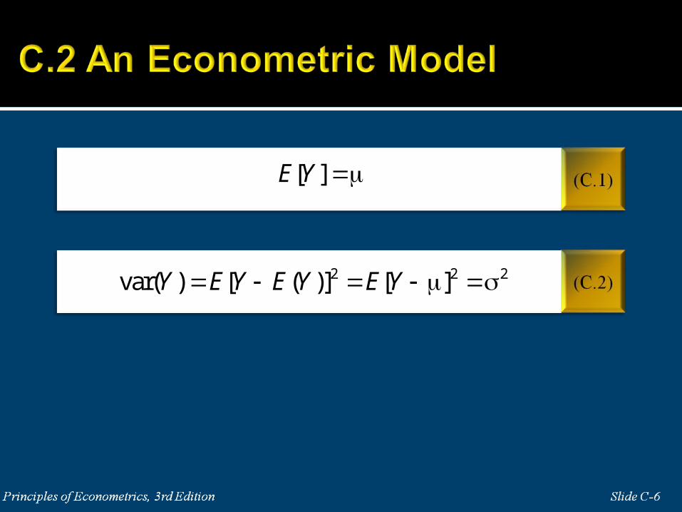
[ ]E Y

2 2 2var( ) [ ( )] [ ]Y E Y E Y E Y

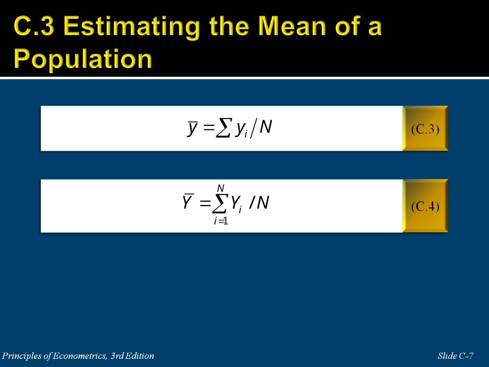
iy y N

1

/ N

ii

Y Y N

iy y N

1

/ N

ii

Y Y N

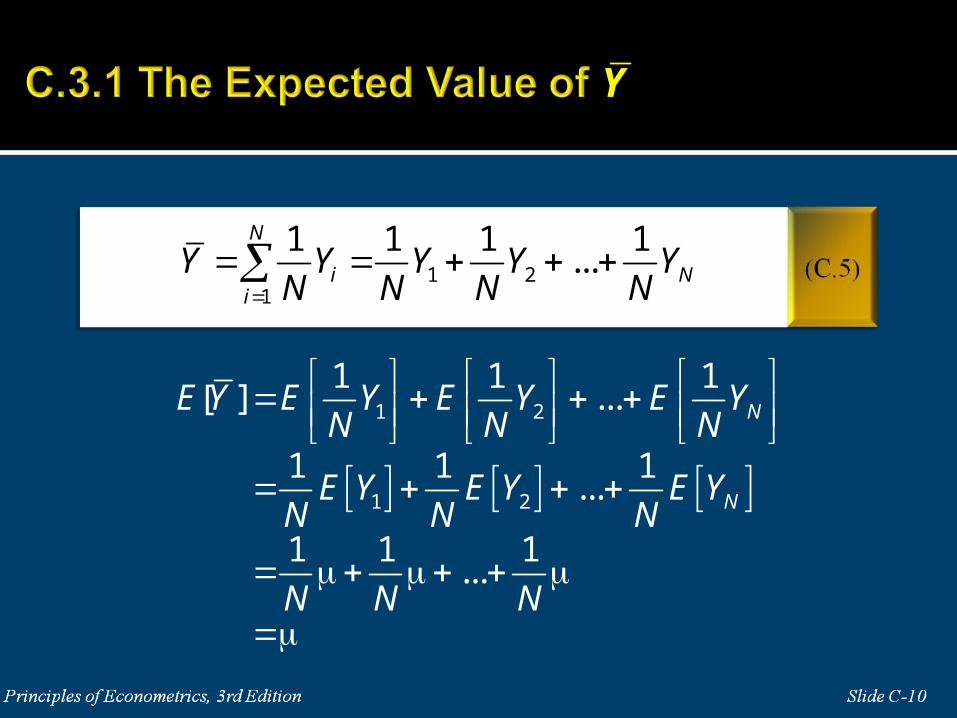
1 21

1 1 1 1...

N

i Ni

Y Y Y Y YN N N N

Y

1 2

1 2

1 1 1[ ] ...

1 1 1...

1 1 1...

N

N

E Y E Y E Y E YN N N

E Y E Y E YN N N

N N N

Y

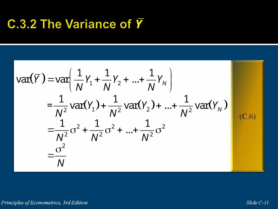
1 2

1 22 2 2

2 2 22 2 2

2

1 1 1var var ...

1 1 1= var var ... var

1 1 1 ...

N

N

Y Y Y YN N N

Y Y YN N N

N N N

N

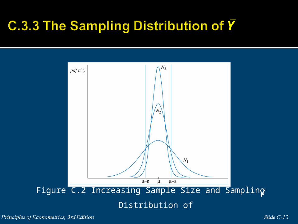
Figure C.2 Increasing Sample Size and Sampling Distribution of

Y

Y

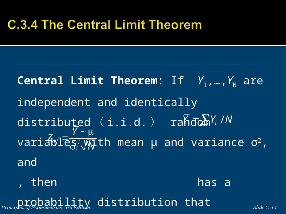
Central Limit Theorem: If Y1,…,YN are independent

and identically distributed （ i.i.d. ） random variables

with mean μ and variance σ2, and

, then has a probability distribution that

converges to the standard normal N(0,1) as N .

/iY Y NN

YZ

N

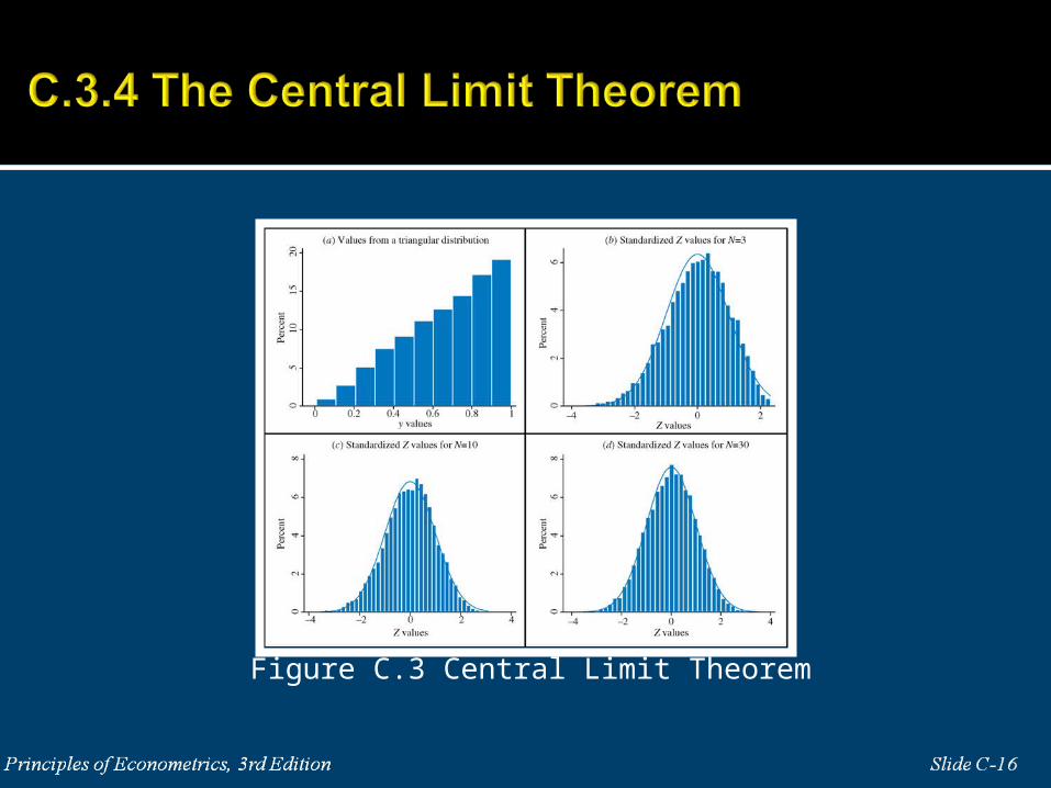
Figure C.3 Central Limit Theorem

A powerful finding about the estimator of the population mean is that it is the best of all possible estimators that are both linear and unbiased( 線性不偏 ).

A linear estimator is simply one that is a weighted average of the Yi’s, such as , where the ai are constants.

“Best” means that it is the linear unbiased estimator with the smallest possible variance.

i iY a Y

rr E Y

1

1 0E Y E Y

2 22

3

3

4

4

E Y

E Y

E Y

22

2

2

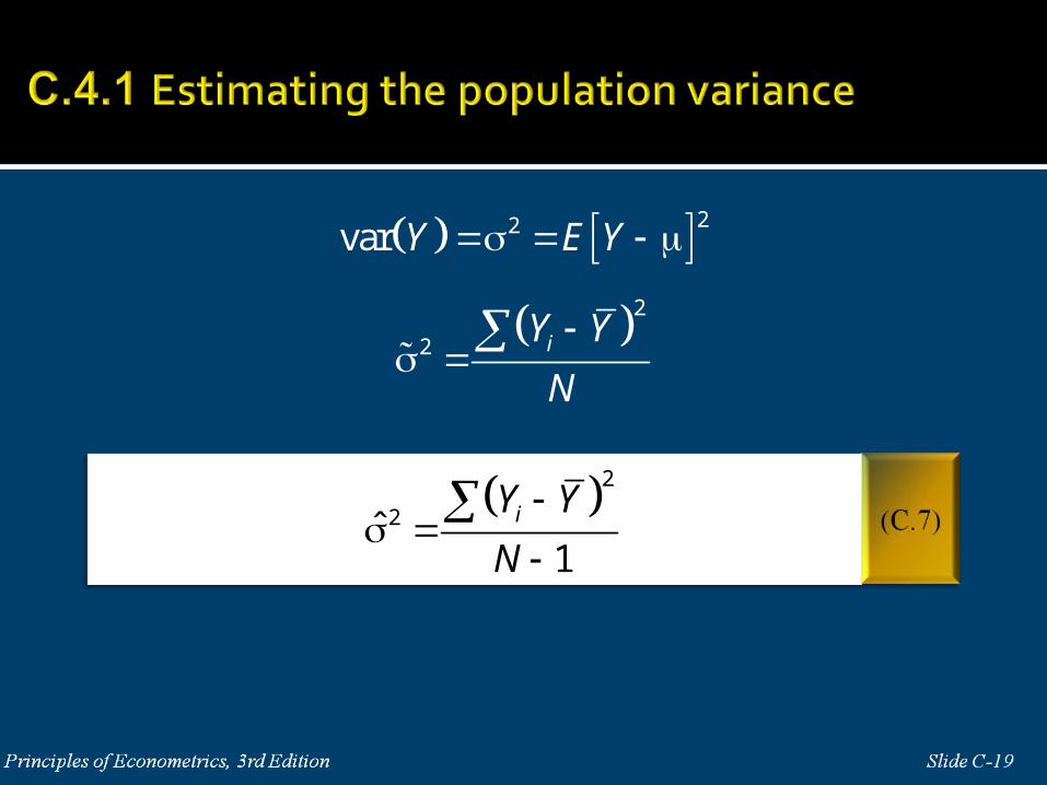
var

i

Y E Y

Y Y

N

22ˆ1

iY Y

N

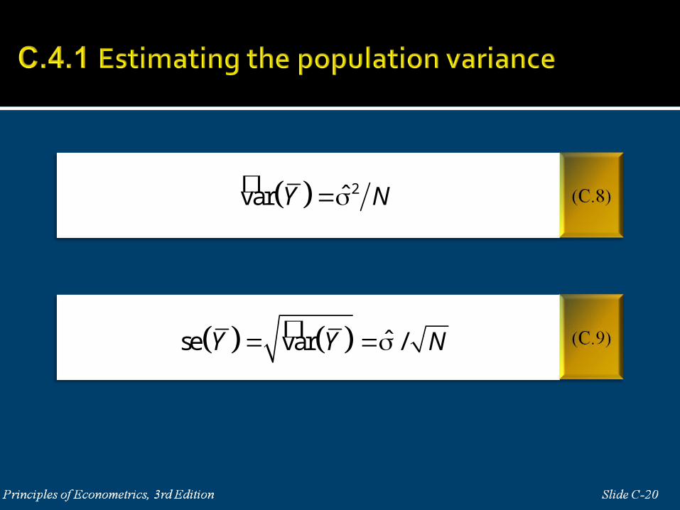
2ˆvar Y N

ˆse var /Y Y N

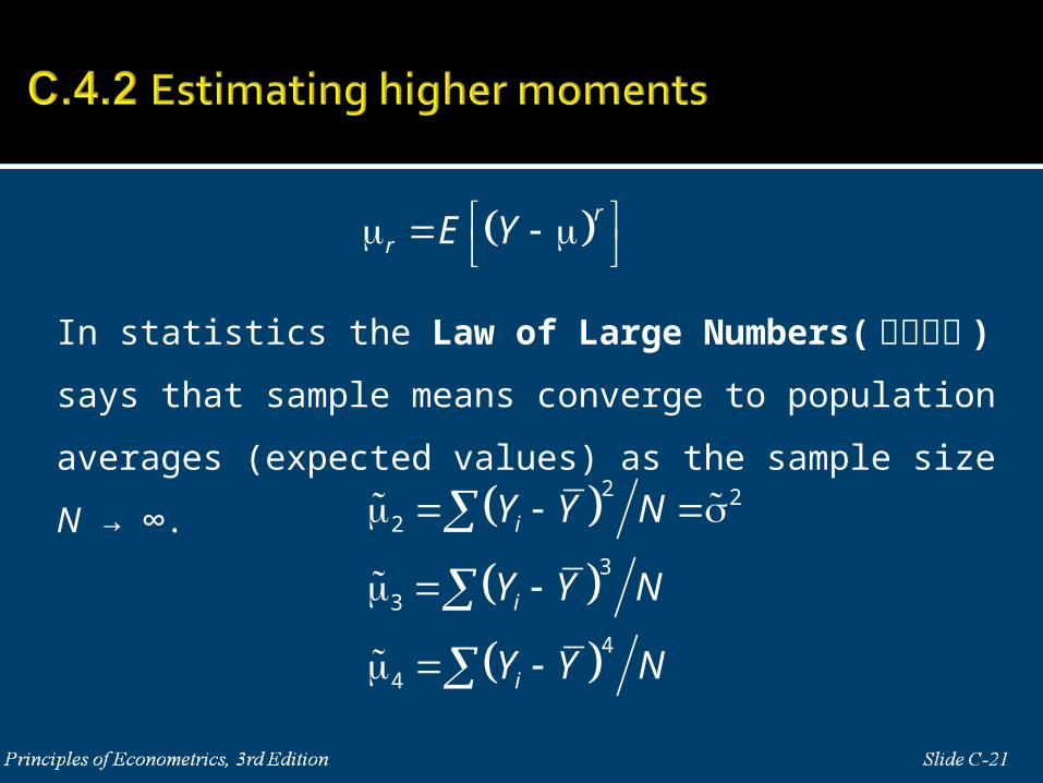
In statistics the Law of Large Numbers(大數法則 ) says that

sample means converge to population averages (expected values) as

the sample size N → ∞.

rr E Y

2 22

3

3

4

4

i

i

i

Y Y N

Y Y N

Y Y N

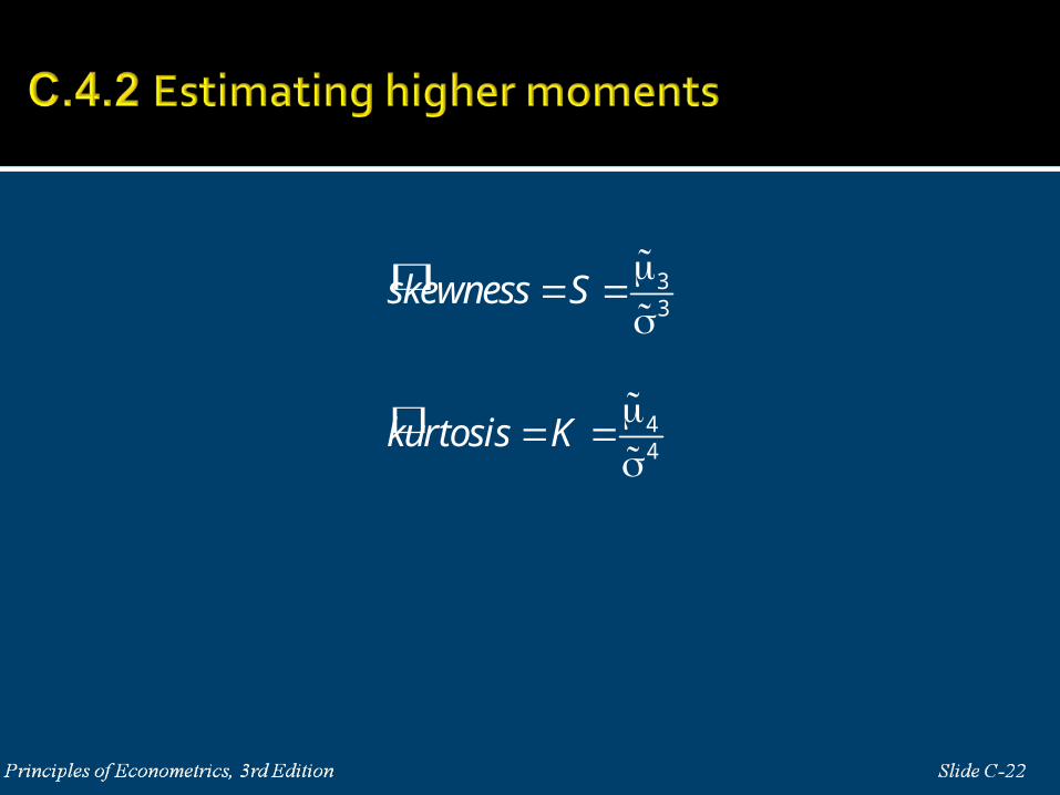
33

44

skewness S

kurtosis K

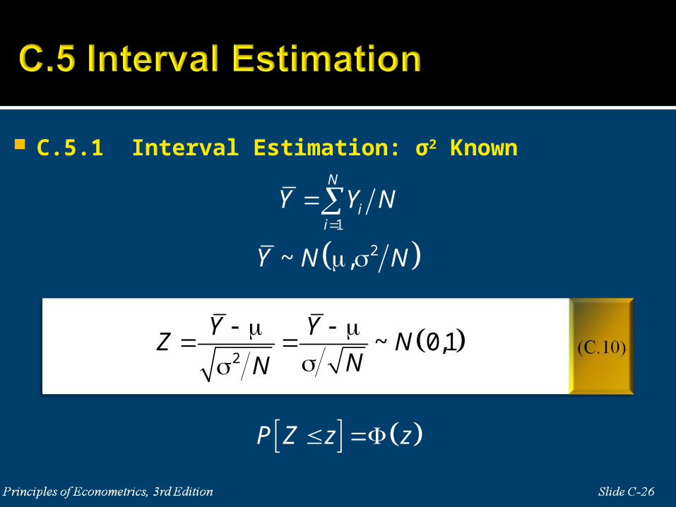
C.5.1 Interval Estimation: σ2 Known

1

2~ ,

N

ii

Y Y N

Y N N

2

~ 0,1Y Y

Z NNN

P Z z z

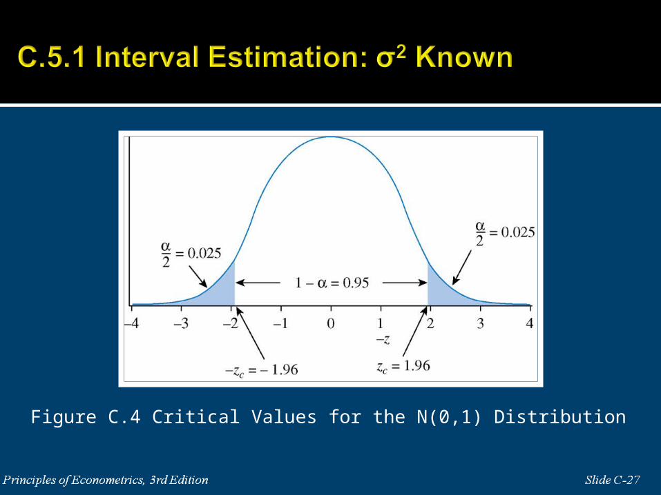
Figure C.4 Critical Values for the N(0,1) Distribution

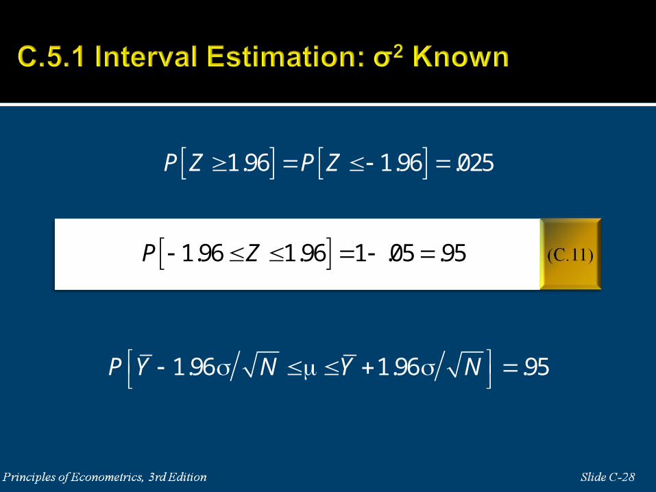
1.96 1.96 .025P Z P Z

1.96 1.96 1 .05 .95P Z

1.96 1.96 .95P Y N Y N

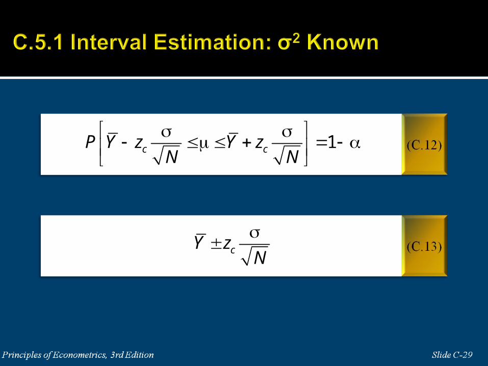
1c cP Y z Y zN N

cY zN

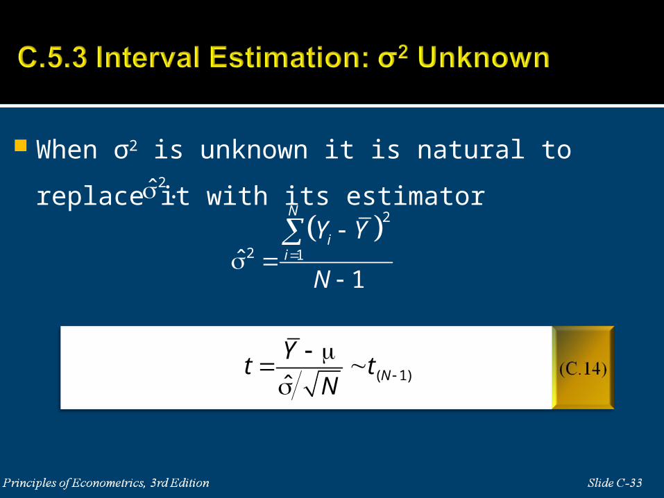
When σ2 is unknown it is natural to replace it with its

estimator 2ˆ .

22 1ˆ

1

N

ii

Y Y

N

( 1)ˆ N

Yt t

N

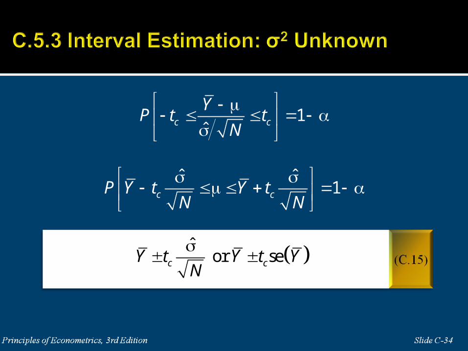
1ˆ

ˆ ˆ1

c c

c c

YP t t

N

P Y t Y tN N

ˆ or sec cY t Y t Y

N

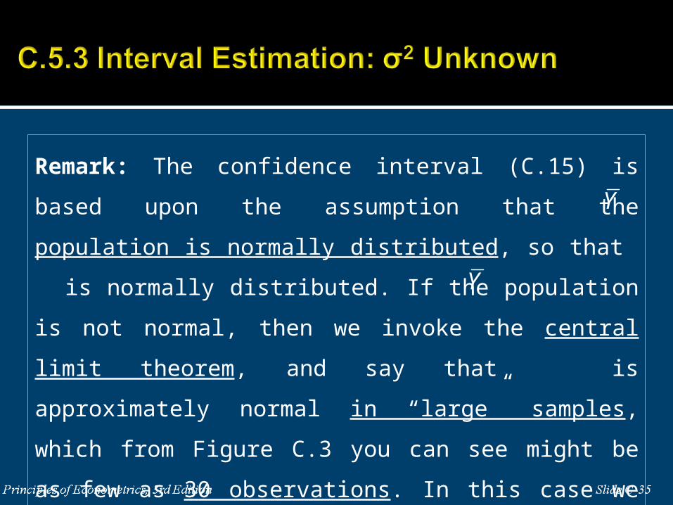
Remark: The confidence interval (C.15) is based upon the

assumption that the population is normally distributed, so that is

normally distributed. If the population is not normal, then we

invoke the central limit theorem, and say that is approximately

normal in “large” samples, which from Figure C.3 you can see

might be as few as 30 observations. In this case we can use (C.15),

recognizing that there is an approximation error introduced in

smaller samples.

Y

Y

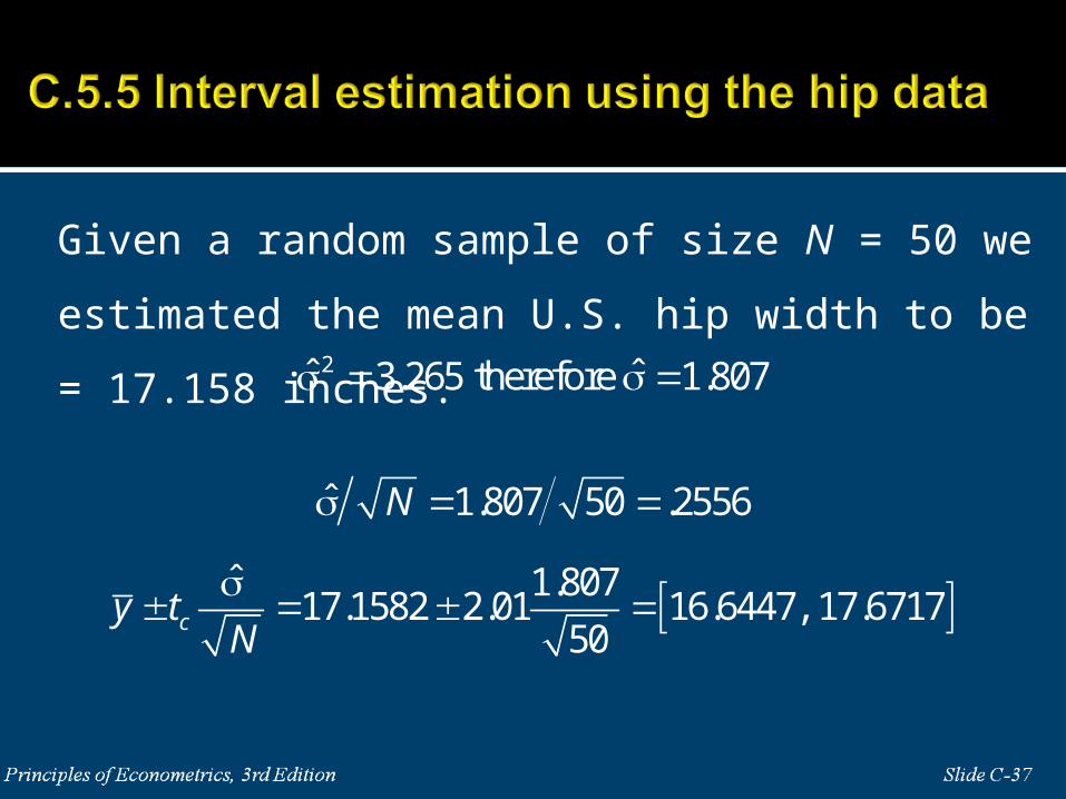
Given a random sample of size N = 50 we estimated the

mean U.S. hip width to be = 17.158 inches. 2ˆ ˆ3.265 therefore 1.807

ˆ 1.807 50 .2556N

ˆ 1.80717.1582 2.01 16.6447, 17.6717

50cy t

N

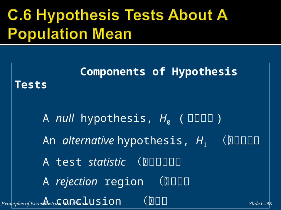
Components of Hypothesis Tests 

A null hypothesis, H0 ( 虛無假設 )

An alternative hypothesis, H1 （對立假設）

A test statistic （檢定統計量）A rejection region （拒絕域）A conclusion （結論）

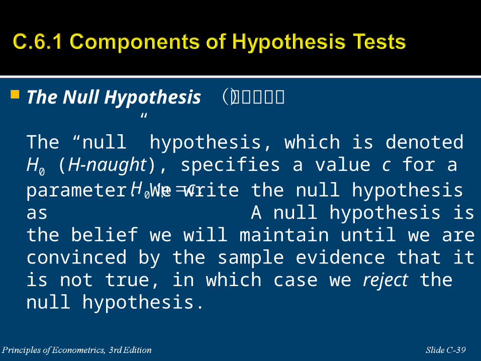
The Null Hypothesis （虛無假設） 

The “null” hypothesis, which is denoted H0 (H-naught), specifies a value c for a parameter. We write the null hypothesis as A null hypothesis is the belief we will maintain until we are convinced by the sample evidence that it is not true, in which case we reject the null hypothesis.

0 : .H c

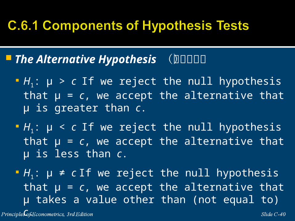
The Alternative Hypothesis （對立假設）

H1: μ > c If we reject the null hypothesis that μ = c, we accept the alternative that μ is greater than c.

H1: μ < c If we reject the null hypothesis that μ = c, we accept the alternative that μ is less than c.

H1: μ ≠ c If we reject the null hypothesis that μ = c, we accept the alternative that μ takes a value other than (not equal to) c.

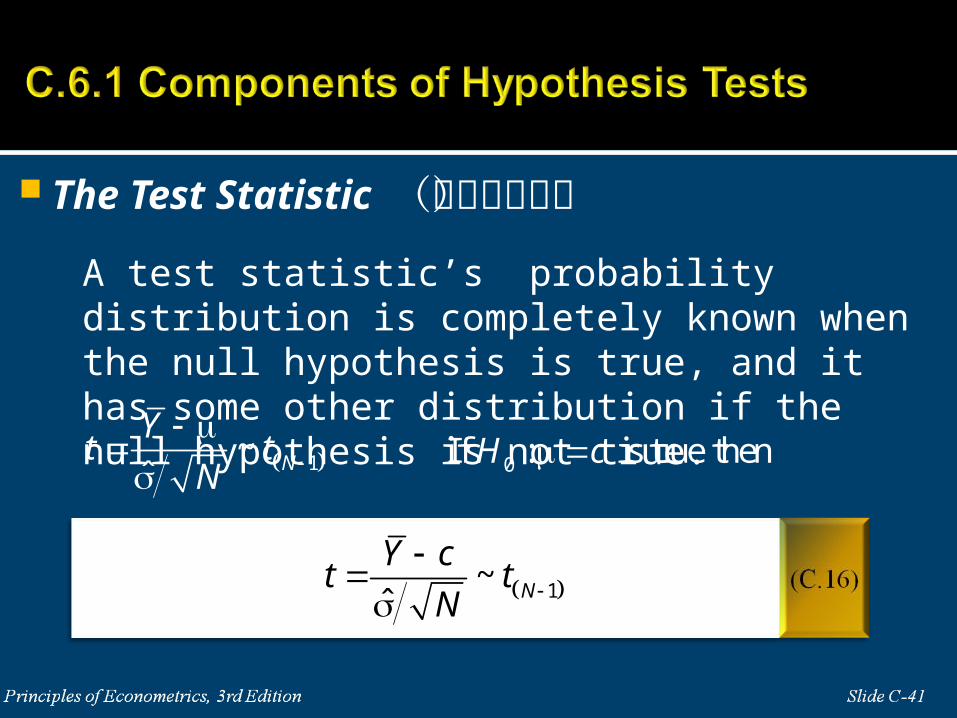
The Test Statistic （檢定統計量）

A test statistic’s probability distribution is completely known when the null hypothesis is true, and it has some other distribution if the null hypothesis is not true.

1~ˆ N

Yt t

N

1~ˆ N

Y ct t

N

0If : is true thenH c

Remark: The test statistic distribution in (C.16) is based on an assumption that the population is normally distributed. If the population is not normal, then we invoke the central limit theorem, and say that is approximately normal in “large” samples. We can use (C.16), recognizing that there is an approximation error introduced if our sample is small.

Y

The Rejection Region

 If a value of the test statistic is obtained that falls in a region of low probability, then it is unlikely that the test statistic has the assumed distribution, and thus it is unlikely that the null hypothesis is true.

If the alternative hypothesis is true, then values of the test statistic will tend to be unusually “large” or unusually “small”, determined by choosing a probability , called the level of significance of the test.

The level of significance （顯著水準 ） of the test is usually chosen to be .01, .05 or .10.

A Conclusion

 When you have completed a hypothesis test you should state your conclusion, whether you reject, or do not reject, the null hypothesis.

Say what the conclusion means in the economic context of the problem you are working on, i.e., interpret the results in a meaningful way.

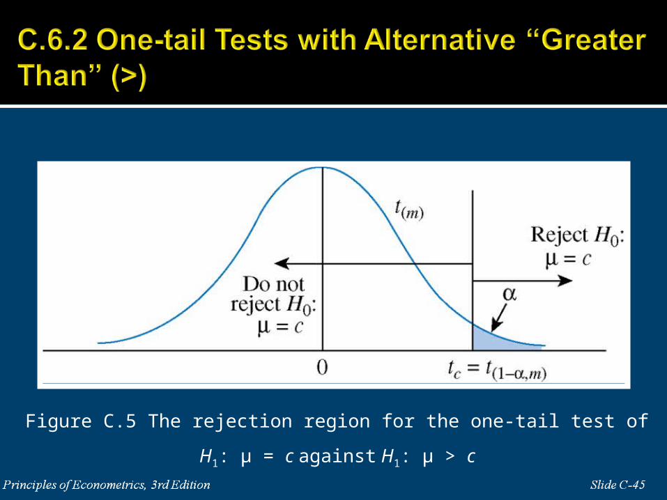
Figure C.5 The rejection region for the one-tail test of H1: μ = c against H1: μ > c

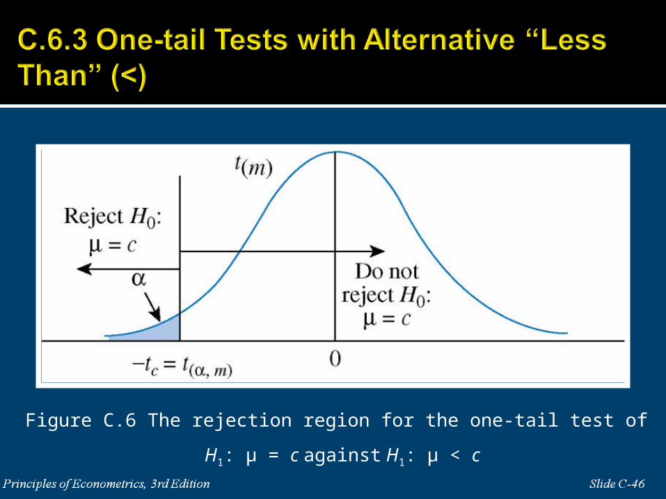
Figure C.6 The rejection region for the one-tail test of H1: μ = c against H1: μ < c

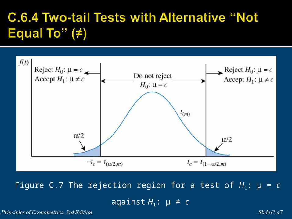
Figure C.7 The rejection region for a test of H1: μ = c against H1: μ ≠ c

The null hypothesis isThe alternative hypothesis is

The test statistic if the null hypothesis is true.

The level of significance =.05.

0 : 16.5.H

1 : 16.5.H

( 1)

16.5~

ˆ N

Yt t

N

.95,49 1.6766ct t

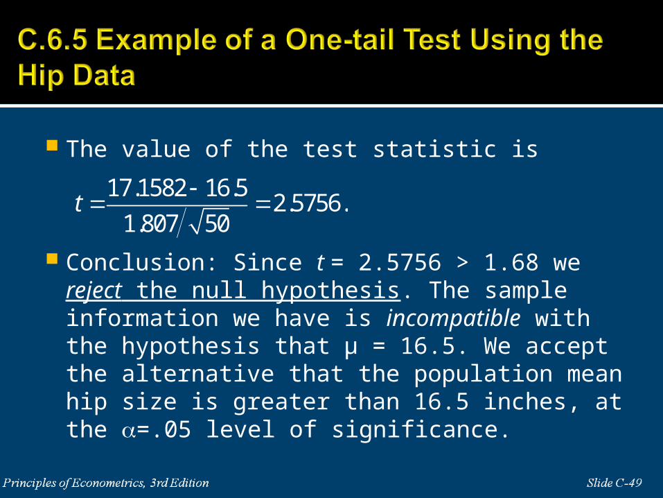
The value of the test statistic is

Conclusion: Since t = 2.5756 > 1.68 we reject the null hypothesis. The sample information we have is incompatible with the hypothesis that μ = 16.5. We accept the alternative that the population mean hip size is greater than 16.5 inches, at the =.05 level of significance.

17.1582 16.52.5756.

1.807 50t

The null hypothesis isThe alternative hypothesis is

The test statistic if the null hypothesis is true.

The level of significance =.05, therefore

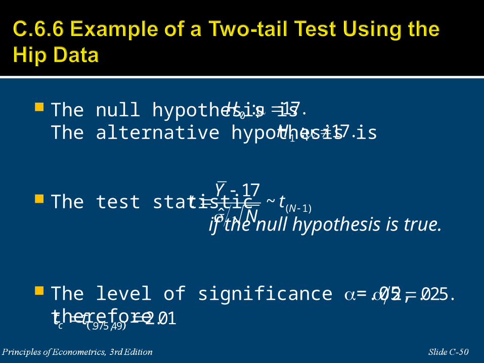
0 : 17.H

1 : 17.H

( 1)

17~

ˆ N

Yt t

N

.975,49 2.01ct t 2 .025.

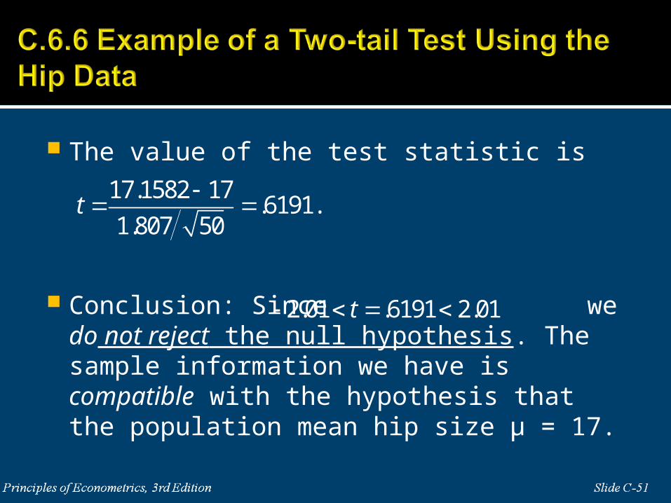
The value of the test statistic is

Conclusion: Since we do not reject the null hypothesis. The sample information we have is compatible with the hypothesis that the population mean hip size μ = 17.

17.1582 17.6191.

1.807 50t

2.01 .6191 2.01t

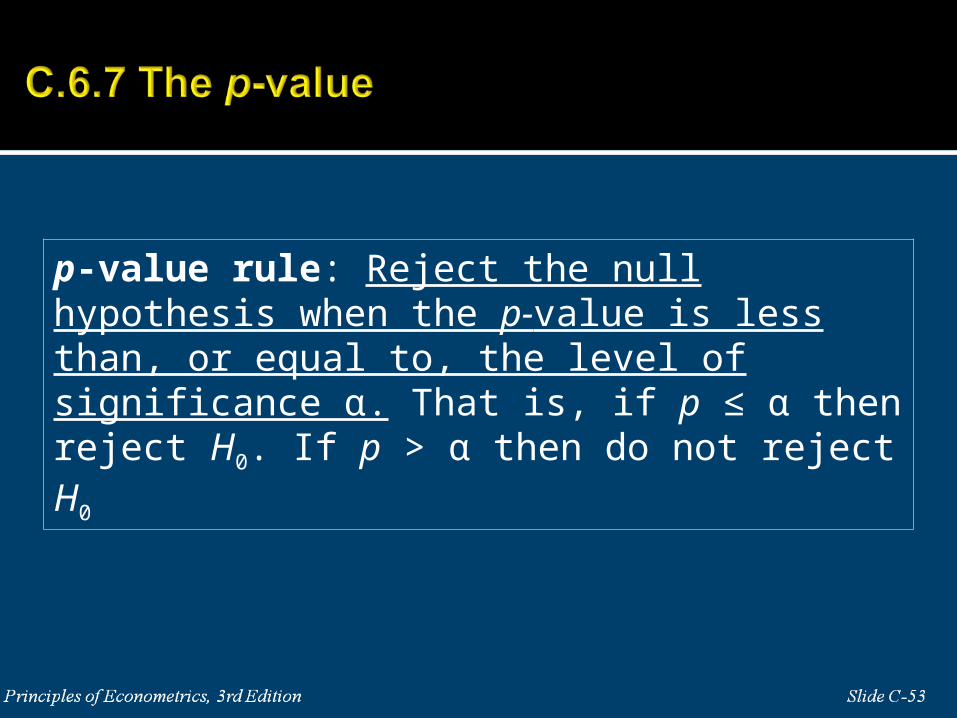
p-value rule: Reject the null hypothesis when the p-value is less than, or equal to, the level of significance α. That is, if p ≤ α then reject H0. If p > α then do not reject H0

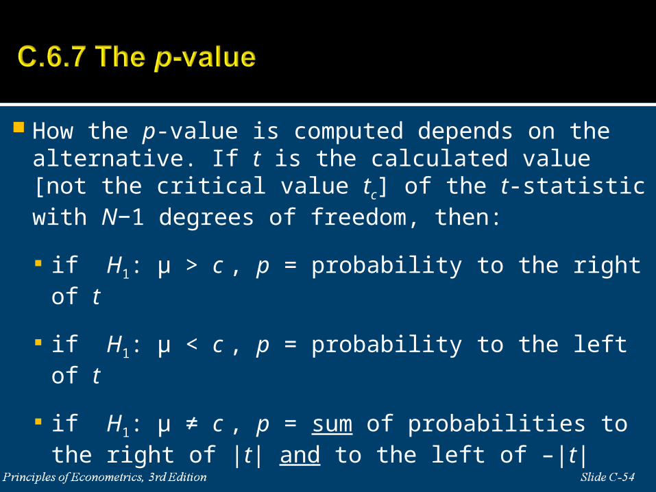
How the p-value is computed depends on the alternative. If t is the calculated value [not the critical value tc] of the t-statistic with N−1 degrees of freedom, then:

if H1: μ > c , p = probability to the right of t

if H1: μ < c , p = probability to the left of t

if H1: μ ≠ c , p = sum of probabilities to the right of |t| and to the left of –|t|

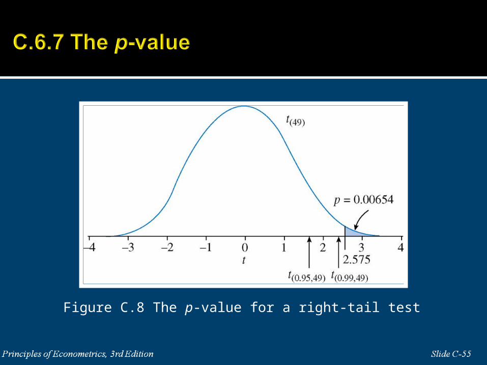
Figure C.8 The p-value for a right-tail test

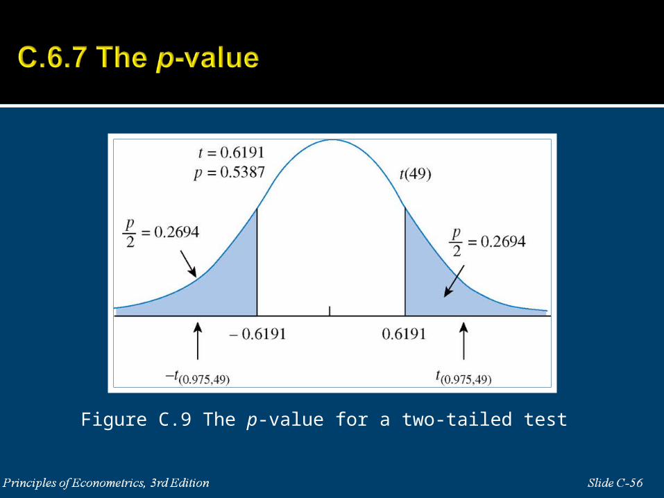
Figure C.9 The p-value for a two-tailed test

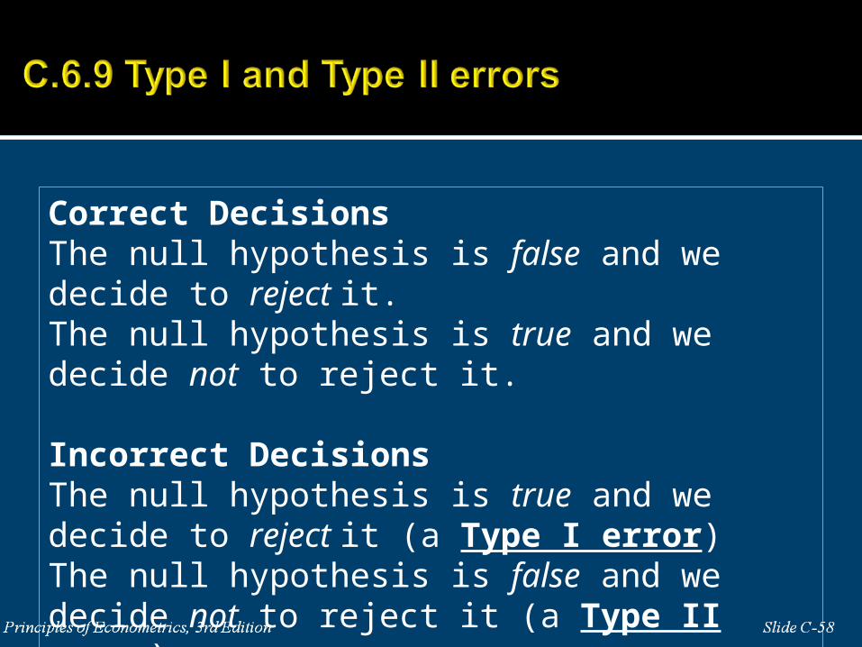
Correct DecisionsThe null hypothesis is false and we decide to reject it.The null hypothesis is true and we decide not to reject it.

Incorrect DecisionsThe null hypothesis is true and we decide to reject it (a Type I error)The null hypothesis is false and we decide not to reject it (a Type II error)

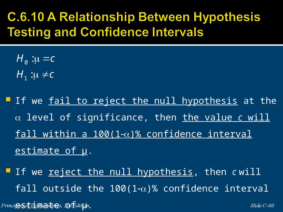
If we fail to reject the null hypothesis at the level of significance,

then the value c will fall within a 100(1)% confidence interval

estimate of μ.

If we reject the null hypothesis, then c will fall outside the 100(1)%

confidence interval estimate of μ.

0

1

:

:

H c

H c

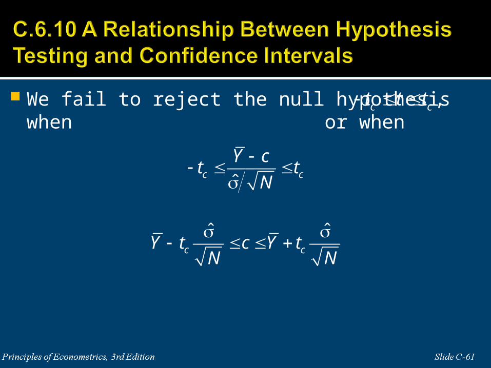
We fail to reject the null hypothesis when or when

,c ct t t

ˆc c

Y ct t

N

ˆ ˆc cY t c Y t

N N

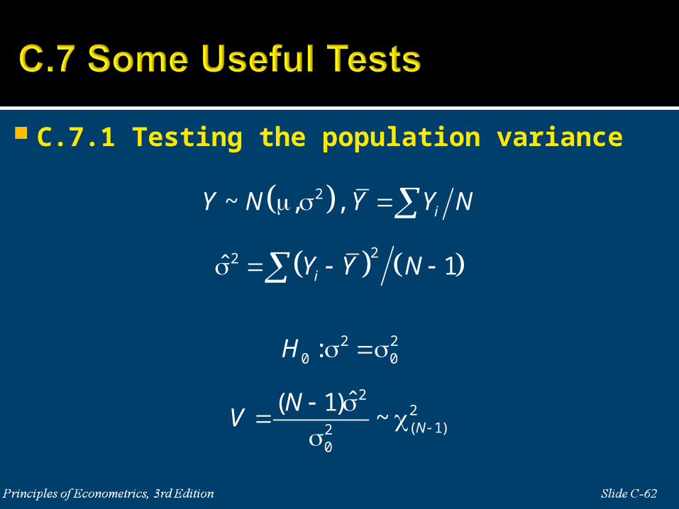
C.7.1 Testing the population variance

2

22

2 20 0

22( 1)2

0

~ , ,

ˆ 1

:

ˆ( 1)~

i

i

N

Y N Y Y N

Y Y N

H

NV

2 21 0

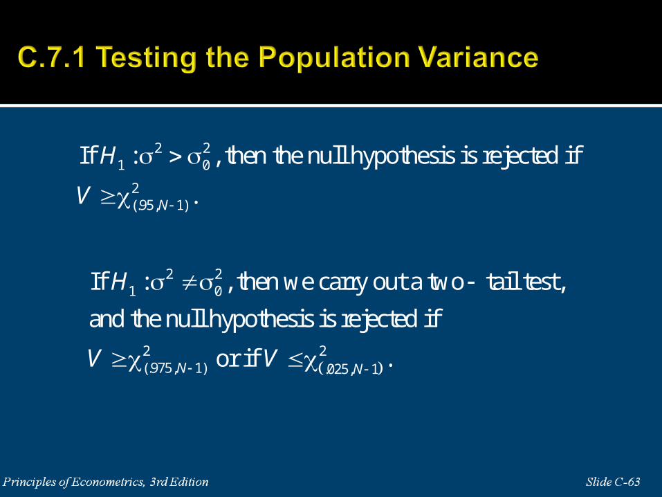
2(.95, 1)

If : , then the null hypothesis is rejected if

.N

H

V

2 21 0

2 2(.975, 1) .025, 1

If : , then we carry out a two tail test,

and the null hypothesis is rejected if

or if .N N

H

V V

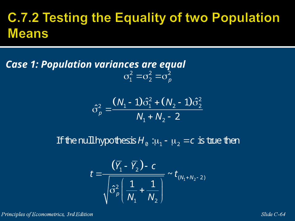
Case 1: Population variances are equal

1 2

2 2 21 2

2 21 1 2 22

1 2

0 1 2

1 2

( 2)

2

1 2

ˆ ˆ1 1ˆ

2

If the null hypothesis : is true then

~1 1

ˆ

p

p

N N

p

N N

N N

H c

Y Y ct t

N N

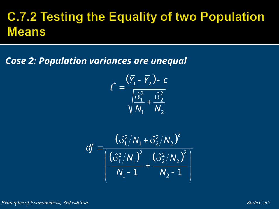
Case 2: Population variances are unequal

1 2*

2 21 2

1 2

22 21 1 2 2

2 22 21 1 2 2

1 2

ˆ ˆ

ˆ ˆ

ˆ ˆ

1 1

Y Y ct

N N

N Ndf

N N

N N

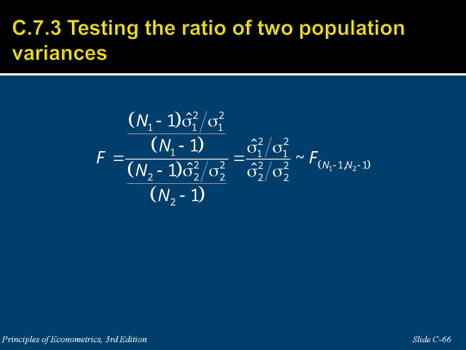
1 2

2 21 1 1

2 21 1 1

2 2 1, 12 22 2 2 2 2

2

ˆ1

1 ˆ~

ˆ ˆ1

1

N N

N

NF F

N

N

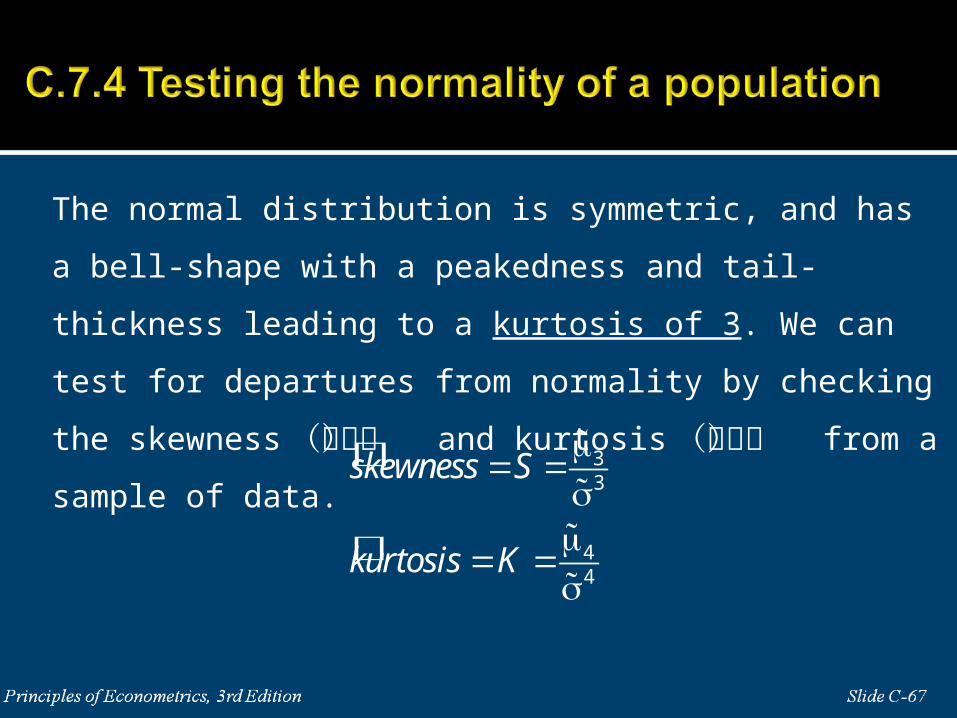
The normal distribution is symmetric, and has a bell-shape with a

peakedness and tail-thickness leading to a kurtosis of 3. We can test

for departures from normality by checking the skewness （偏態） and kurtosis （峰態） from a sample of data.

33

44

skewness S

kurtosis K

Slide C-56Principles of Econometrics, 3rd Edition