Embed Size (px)
Citation preview

777 SOUTH FIGUEROA STREET, SUITE 1950 LOS ANGELES, CALIFORNIA 90017 TEL: 213.346.3000 FAX: 213.346.3030
White Plains, NY / Washington, DC / Los Angeles, CA / Cambridge, MA / Philadelphia, PA / San Francisco, CA / New York, NY / Ithaca, NY / Seattle, WA / London / Madrid
REVIEW OF TIME-OF-USE AND INVERTED ELECTRIC RATE STRUCTURES FOR APPLICATION IN MANITOBA
Prepared by
Hethie S. Parmesano
Amparo Nieto
William F. Rankin
Veronica Irastorza
July 28, 2005
Cost of Service Methodology Review PUB - MFR 2


TABLE OF CONTENTS
EXECUTIVE SUMMARY .........................................................................................................I
I. INTRODUCTION .......................................................................................................... 1
II. RATIONALE FOR INVERTED AND TOU RATES................................................. 2
A. Economic Efficiency ...................................................................................................................................2
B. Promotion of Cost-Effective Conservation ..............................................................................................6
C. Improving Intra-Class Rate Equity ..........................................................................................................7
D. Other Rate Objectives................................................................................................................................8
III. USE OF TOU AND INVERTED RATES BY OTHER UTILITIES......................... 8
A. Seasonality and Time-of-Day Rates..........................................................................................................9
B. Real-Time Pricing Structures....................................................................................................................9
C. Existing and Proposed Inverted Block Rates...........................................................................................9
IV. FACTORS IN MANITOBA AFFECTING TOU AND INVERTED RATES........ 11
A. Predominantly Hydro-Electric System...................................................................................................12
B. Importance of Energy Exports................................................................................................................13
C. Manitoba Hydro’s Marginal Costs .........................................................................................................14
D. Relationship between Embedded Costs and Marginal Cost Revenues................................................20
E. Metering and Billing Capabilities ...........................................................................................................21
V. FRAMEWORK FOR COST-BENEFIT EVALUATION OF TOU AND INVERTED RATES..................................................................................................... 23
A. Interrelated Impacts of Rate Structure Changes ..................................................................................23
B. Changes in Costs, Revenue Requirement and Class Revenue Allocation ...........................................25
C. Economic Implications of Rate Structure Changes...............................................................................26

REVIEW OF TIME-OF-USE AND
INVERTED RATES VI. ALTERNATIVE RATE STRUCTURES FOR REVIEW........................................ 27
A. Seasonal Rates ..........................................................................................................................................28
B. TOD Unblocked Rates .............................................................................................................................28
C. Inverted Block Rates ................................................................................................................................29
D. Optional Rate Structures Tested for Manitoba Hydro Customers .....................................................32
E. Illustrative Charges under each Rate Scenario .....................................................................................34
VII. ANALYSIS OF ILLUSTRATIVE RATES................................................................ 43
A. Changes in Consumption Based on Elasticity Estimates and Feedback to Illustrative Rates...........43
B. Effect of TOD and Inverted Rates on Manitoba Hydro’s Revenue Requirement .............................46
C. Welfare Assessment of TOD and Inverted Rates Tested for Manitoba Hydro Customers...............49
D. Bill Impact Analysis under each of the Illustrative Rates ....................................................................53
VIII. CONCLUSIONS AND RECOMMENDATIONS ..................................................... 69
IX. NEXT STEPS................................................................................................................ 71
APPENDIX A. SURVEY ELECTRICITY RATE STRUCTURES IN NORTH AMERICA.................................................................................................................................72
APPENDIX B. MANITOBA HYDRO CURRENT RATES (APRIL 1, 2005) ...................80
APPENDIX C. ILLUSTRATIVE RATES AND AVERAGE MONTHLY BILL COMPARISONS ......................................................................................................................83
NERA Economic Consulting

EXECUTIVE SUMMARY
INTRODUCTION The Manitoba Public Utilities Board (PUB) directed Manitoba Hydro to prepare a report evaluating the appropriateness of implementing (1) inverted rates and (2) time-of-use (TOU) rates for electricity consumers in Manitoba.1 Manitoba Hydro engaged NERA Economic Consulting to prepare the required report, with assistance from Manitoba Hydro staff.
Both inverted and TOU rates offer the potential to give better signals to consumers about the cost consequences of their electricity consumption decisions. In the case of TOU rates, prices vary by season and (if metering permits) time-of-day (TOD). In the case of inverted rates, prices for the run-off rate can be set closer to cost, with the earlier block or blocks priced to recover the remaining revenue requirement. These rate structures are typically proposed for one or more of the following reasons:
• Improving economic efficiency, by pricing so that consumers face prices for marginal consumption that approximate the marginal costs of service;
• Promoting cost-effective conservation, thus reducing the need for conservation subsidies;
• Improving intra-class rate equity;
• Promoting renewables and distributed generation because bill savings to consumers investing in these technologies could be large if consumption in the run-off block or peak hours is reduced;
• Increasing customer choice, by giving customers flexibility in the way they manage their energy costs.
• Reducing financial risk for the utility, by setting prices that track the underlying costs.
Most of these reasons for using inverted and TOU rate structures assume that the rates will reflect the utility’s marginal cost of service. For purposes of this report, we worked with Manitoba Hydro to develop illustrative rates under a number of alternative rate structures for each rate class, taking into account Manitoba Hydro’s marginal costs of generation, transmission and demand-related distribution and the required revenue reconciliation to meet Manitoba Hydro’s revenue requirement by class. Charging marginal costs directly as prices would produce too much revenue. Overall, Manitoba Hydro’s marginal cost revenues exceed
NERA Economic Consulting
1 PUB Order 7/03.
i

current retail revenues by about 43 percent.2 For inverted rate structures, the early block or blocks can be set below marginal cost to produce the correct revenue. For TOD rates without blocking, the TOD prices must be distorted to some degree to produce the right revenue (and to prevent unacceptable bill impacts.)
USE OF TIME-OF-USE AND INVERTED RATES BY OTHER UTILITIES
As part of our assignment we undertook a survey of rate structures at selected utilities across North America, with particular emphasis on those with cost structures, operating regimes, and customer characteristics similar to those of Manitoba Hydro:
• Avista
• BC Hydro
• Hydro One
• Hydro Quebec
• Idaho Power
• Newfoundland and Labrador Hydro
• Northern States Power
• Pacificorp (WA and OR)
• Portland General Electric
• Puget Sound
• Salt River Project
• Seattle City Light
Five of the twelve surveyed utilities have seasonal rates. TOD structures are less common; they usually take the form of optional or experimental rates. Only three utilities make TOD rates mandatory, and then only for large general service customers.
Inverted rates are common for residential customers. Eleven of the 12 surveyed utilities have inverted per-kWh charges for at least one residential class. Only three of the utilities (BC Hydro, Hydro One and Idaho Power) have inverted block energy charges for small and medium general service customers. BC Hydro is also proposing two optional inverted rates for its large commercial and industrial customers.3
NERA Economic Consulting
2 This calculation assumes that revenues currently recovered in customer charges are equal to marginal
customer and local distribution facilities costs, which were not calculated for this study. 3 See BC Hydro’s “Transmission Service Rate Application,” March 2005.
ii

EVALUATION OF TOU AND INVERTED RATES Analysis of the impacts of introducing TOU and inverted rates is a complex task because of the interrelationships between rates, loads, costs, and revenue requirements. Changing rate structures affects customer loads, which in turn affect the amount of energy available for export (and export revenues), as well as changes in operating and capital costs. This has an effect on the total revenue requirement to be recovered from rates and its allocation by class, which in turn affects both the level and appropriate rate structure (e.g., peak/off-peak price differentials).
Interrelated Impacts of Rate Structure Changes
Costs:Operating expensesCapital expenditures
Revenue Requirement
Rates:StructureLevel
Loads:Peak demandEnergy by period
Exports
Export Revenues
Electricity
Dollars
Embedded Cost Allocation to Classes
The analysis of alternative rate structures in this report provides estimates of three types of effects: (1) the overall effects on Manitoba Hydro’s costs, which are assumed to be passed through in rate changes; (2) net welfare effects, which include both the rate changes resulting from changes in Manitoba Hydro’s costs and changes in consumer surplus;4 and (3) the effect on bills of customers using particular amounts of energy and capacity.
4 Consumer surplus is the difference between what a consumer pays for a quantity of energy and the value the
consumer receives from that quantity. When a customer responds to a higher price by reducing usage, there is a reduction in consumer surplus. When the customer responds to a lower price by increasing usage, there is a gain in consumer surplus.
NERA Economic Consulting
iii

Steps and Assumptions in Analysis The evaluation process used for this report consists of the following steps:
1. Develop revenue neutral rates using the generic rate structures under study. In the case of inverted block rates or consumer-specific baselines, the run-off rate is set close to marginal cost (subject to social acceptability constraints, as will be explained below). In the case of unblocked TOD rates, some adjustments were made in order to reconcile the class revenue requirement and the revenues that would be generated by charges equal to marginal costs.
2. Estimate the change in consumption for the class, using estimates of demand elasticity. The elasticity estimates are not used to predict changes in demand, but rather to evaluate the relative shifts that might occur with implementation of the various tariff structures.
3. Estimate the change in Manitoba Hydro’s costs resulting from the change in consumption—marginal cost times change in usage by a typical customer in the class. In the case of residential, four typical customer sub-groups were defined, depending on whether they are ‘standard’ electric use (versus electric-space heating) and whether their consumption falls in the current first block or the second block. In the case of GSS-ND, six sub-groups were defined for purposes of the load response analysis, differentiating between those whose marginal consumption falls into the first, second or third blocks of the current rates, and whether they use electric space heating or not.
4. Adjust the class revenue requirement by the amount of Manitoba Hydro’s change in cost.
5. Adjust the illustrative rates to produce the new class revenue requirement.
6. Compute the change in bills for various levels of consumption (holding consumption unchanged).
7. Compute total welfare effects–which include changes in bills and changes in consumer surplus.
Our analysis of illustrative rates using a variety of rate structures depends upon a number of simplifying assumptions:
• Any change in export quantities does not affect the export price (and marginal cost of generation).
• Manitoba Hydro’s current estimates of marginal costs adequately capture the incremental costs and decremental costs of changes in use that might result from new rate structures.
NERA Economic Consulting
iv

• The effects of TOU and inverted rate structures can be approximated by looking at a single representative year.5
• Class revenue requirements, which are initially assumed to be revenues at current rates, are adjusted based on the change in marginal cost revenues that result from changed consumption resulting from the new rate structure, using assumptions about demand elasticity.
• Demand elasticities from studies in other jurisdictions provide a reasonable basis for estimating possible consumer response to changes in rate structure.
• Incremental metering, billing and rate administration costs were not included in the analysis.
Illustrative Rates Examined A number of specific rate structures were evaluated: seasonal rates (which require no special metering), TOD rates (which are also seasonal) with and without demand charges, and inverted block rates. The TOU rates use the following period definitions:
Summer: June through SeptemberPeak Period: 12:00 Noon to 8:00 pm WeekdaysShoulder Period: 7:00 am to 12:00 noon; 8:00 pm to 11:00 pm Weekdays.
7:00 am to 11:00 pm WeekendsOff Peak Period: 11:00 pm to 7:00 am all days
Fall: October through NovemberWinter: December through MarchSpring: April through May
Peak Period: 7:00 to 11:00 am; 4:00 pm to 8:00 pm WeekdaysShoulder Period: 11:00 am to 4:00 pm; 8:00 pm to 11:00 pm Weekdays
7:00 am to 11:00 pm WeekendsOff Peak Period: 11:00 pm to 7:00 am all days
Inverted block rates can provide efficient price signals because the run-off rate can be set at or close to marginal cost, and the first block set to recover the remaining revenue requirement. The size of the first block determines how many customers are exposed to the
5 This single-year “snapshot” approach relies on rather short-run estimates of customer response to new rate
structures, but uses long-term estimates of the cost effects (and revenue requirement effects) of these changes.
NERA Economic Consulting
v

efficient run-off rate; if the first block is too large, few customers will face the efficient price. We evaluated two types of inverted block rates for residential customers:
• Scenario 1 - separate non-seasonal first block sizes were defined for standard customers (without electric space heating) and seasonal first block sizes for customers with electric space heating (“All-electric”).
• Scenario 2 - the same first block sizes (which vary by season) apply to all residential customers.
We also evaluated two types of inverted block rates for non-residential customers. Inverted rates with blocks defined in terms of specific amounts of kWh are difficult to apply fairly to commercial and industrial customers because the low-cost block proportionally provides a larger benefit to small customers within the class than to large customers. Two competing companies of different sizes would face very different average electricity costs per kWh simply because of the rate structure. This would create a distortion in their competitive positions. The inverted block rates evaluated for non-residential customers included a fixed kWh first block structure only for General Service Small Non-Demand (GSS-ND) customers. All other inverted block structures tested for non-residential customers define a customer-specific first block equal to 90% (75% for GSS-ND customers) of consumption in the base year (“customer baseline” or “CBL”). The CBL would not change except under extraordinary circumstances.6 Under this approach, each commercial or industrial customer pays the low price for a fixed percentage of baseline usage, and the higher tail-block price for all additional usage. This places large and small customers in the class on a more equal footing.
The options tested for each class are summarized in the table below, specifying the structure for energy and demand charges. Customer charges were maintained at their current levels.7 The table also indicates adjustments made to marginal cost levels to reconcile marginal cost revenues with class revenue requirement, as well as to reduce large bill impacts and ensure social acceptability. As an example, the winter peak marginal cost was often adjusted down by a larger amount than other periods, as Manitoba Hydro considered winter charges at full marginal cost to be unacceptable to customers and difficult for the Provincial Government to support. Therefore the illustrative rates for some customers may show both first block and run-off prices below marginal cost. Maximizing simplicity and customer acceptance might require simpler rate structures; e.g., two seasonal pricing periods instead of four. However, simplification involves some sacrifice of efficient price signals. For example, averaging costs to create two seasons instead of four mutes the price signal in the high-cost months. With any change in rate structure, carefully
NERA Economic Consulting
6 Such as a major change in scale of operation. 7 Electric BMC is $6.25 for Residential and $15.75 for GS Small.
vi

designed programs that inform customers of the coming changes and how they can adapt to them are important. Gradual implementation of new structures (and other transition mechanisms) may also be appropriate.
NERA Economic Consulting
vii

ENERGY CHARGES DEMAND CHARGES
Class kWh Structure Block Sizes TD kVA Structure TD
ADJUSTMENT FOR REVENUE
RECONCILIATION
RESIDENTIAL
Scenario 1 Inverted 2-block rates, differentiating between standard customers and All electric. Run-off charge close to MC.
First block for standard: 600kWh; for electric cust: first block size varies by season (600-1,500 kWh)
4 seasons NA NA Winter Peak run-off charges set near MC; all other run off charges set slightly above seasonal MC; first block charge below MC.
Scenario 2 Inverted 2-block rates; same block size for all customers. Mg cost for run off charge.
Same first block size for all residential customers: size varies by season (800-1,000 kWh)
4 seasons NA NA MC for run-off charges; all adjustments made in the first block charge.
GENERAL SERVICE, SMALL, NON-DEMAND METERED
Scenario 1 Winter customer-specific baseline; winter run-off charge close to seasonal MC.
Customer-specific baseline set as 75% of baseline usage
4 seasons NA NA Winter peak run-off charges close to MC; all other set above seasonal MCs. Unblocked charges for the non-winter months.
Scenario 2 Unblocked TOD kWh NA 4 seasons, 3 TOD
NA NA Winter Peak period charge close to MC. Other period charges adjusted down proportionally.
Scenario 3 Inverted two-block rates; run-off charge close to seasonal MC.
Same first block size for all GS-ND customers (6,000 kWh)
4 seasons NA NA Winter Peak run-off charges close to MC; all other set slightly above seasonal MC. First block charge slightly below run-off charge.
GENERAL SERVICE SMALL, MEDIUM AND LARGE (DEMAND-METERED)
Scenario 1 Two blocks, with seasonal MC charge for run-off charge
First block based on customer-specific baseline use (e.g., 90% of base year usage)
4 seasons Demand charge, first 50 kVA free
4 seasons, combined peak & shoulder
Winter kWh and kVA charges below MC. Other kWh charges slightly above MC.
Scenario 2 Two blocks, with TOD run-off charges close to MC
First block based on customer-specific baseline use (90% of base year usage)
4 seasons, 3 TOD periods
Demand charge, first 50 kVA free
4 seasons, combined peak & shoulder
Run-off charges close to MC except for Winter peak, which is set well below MC. CBL charge varies by season to moderate period revenue swings.
Scenario 3 Unblocked TOD kWh NA 4 seasons, 3 TOD
NA NA kWh charges close to MC except for the Winter peak period (<MC) to moderate bill impacts.
Scenario 4 Unblocked TOD kWh NA 4 seasons, 3 TOD
Unblocked demand charges
4 seasons, combined peak & shoulder
Winter kWh and kVA charges below MC. TOU kWh significantly below MC, especially Winter peak charge.
NERA Economic Consulting viii

Effect of TOD and Inverted Rates on Manitoba Hydro’s Costs and Revenue Requirement One measure of the effectiveness of TOD and inverted rate structures is the effect on the utility’s costs and revenue requirement.8 The table below shows the effect on class revenue requirements of each of the rate structures evaluated. These cost impacts are a function of the estimated marginal costs and the assumed demand elasticities, and should be taken as illustrative of possible effects, not as a forecast. Also note that no metering, billing, implementation or rate administration costs are included in the analysis.
Effect of Tariff Structure Change on Manitoba Hydro Costs
(000 $) (%)Scenario 1 (Two rates, two blocks, seasonal) -7,444 -2.0%Scenario 2 (One rate, two blocks, seasonal) -7,420 -2.0%
Scenario 1 (CBL, seasonal run-off charges) -3,830 -3.7%Scenario 2 (No block, TOU kWh) -2,617 -2.6%Scenario 3 (Blocked, seasonal run-off charges) -1,964 -1.9%Scenario 1 (CBL, seasonal kWh, TOU KVA) -4,384 -5.0%Scenario 2 (CBL, TOU kWh, TOU KVA) -7,004 -8.0%Scenario 3 (Unblocked, TOU kWh) -6,526 -7.4%Scenario 4 (Unblocked, TOU kWh, TOU kVA) -5,804 -6.6%
Scenario 1 (CBL, seasonal kWh, TOU KVA) -10,737 -8.0%Scenario 2 (CBL, TOU kWh, TOU KVA) -11,307 -8.4%Scenario 3 (Unblocked, TOU kWh) -1,816 -1.3%Scenario 4 (Unblocked, TOU kWh, TOU kVA) -2,848 -2.1%Scenario 1 (CBL, seasonal kWh, TOU KVA) -2,505 -4.3%Scenario 2 (CBL, TOU kWh, TOU KVA) -4,217 -7.2%Scenario 3 (Unblocked, TOU kWh) -878 -1.5%Scenario 4 (Unblocked, TOU kWh, TOU kVA) -1,406 -2.4%Scenario 1 (CBL, seasonal kWh, TOU KVA) -3,051 -11.6%Scenario 2 (CBL, TOU kWh, TOU KVA) -3,004 -11.5%Scenario 3 (Unblocked, TOU kWh) -1,733 -6.6%Scenario 4 (Unblocked, TOU kWh, TOU kVA) -2,752 -10.5%Scenario 1 (CBL, seasonal kWh, TOU KVA) -20,602 -13.3%Scenario 2 (CBL, TOU kWh, TOU KVA) -19,779 -12.8%Scenario 3 (Unblocked, TOU kWh) -10,511 -6.8%Scenario 4 (Unblocked, TOU kWh, TOU kVA) -15,945 -10.3%
Large GS LV
Large GS MV
Large GS HV
Residential
Small GS ND
Small GS D
Medium GS
Change in Rev Req
8 Revenue Requirement based on the 2005/06 Revenue Requirement using rates effective August 1, 2004.
NERA Economic Consulting
ix

Welfare Assessment of TOD and Inverted Rates Tested for Manitoba Hydro Customers In order to evaluate the full net welfare effects of the illustrative TOD and inverted block structures, it is necessary to take into account not only the reductions in expenditures on electricity, shown in the table above, but also the additional gain (loss) in consumer surplus that occurs when a consumer increases (reduces) consumption. The net annual impacts on welfare by customer class are illustrated in the charts below. All of the scenarios tested produce welfare gains, given the assumptions about rate levels, marginal costs and elasticity values.
• For residential customers, Scenario 2, with a single set of seasonal first blocks, produces higher welfare gains than Scenario 1, which has constant, non-seasonal first block sizes for standard customers and higher (except in summer) seasonally-varying first blocks sizes for all-electric customers.
• For SGS-ND customers, Scenario 2, with TOD energy charges and no blocking,
produces significantly higher welfare gains than the CBL or fixed block structures with no TOD.
• For SGS-D customers, Scenario 2, which combines a 90% CBL block structure with
TOD energy charge produces the largest welfare gains. The two unblocked scenarios (with and without demand charges, respectively) produce welfare gains almost as high. Scenario 1, with a 90% CBL structure but not TOD, has welfare gains much lower.
• The size of welfare gains for GSM and GSL customers follow similar patterns, with
the highest welfare gains from Scenario 2, which has a combination of 90% CBL first block and TOD energy charges. The unblocked TOD scenarios produce higher gains than Scenario 1, which has a 90% CBL feature, but no TOD differentiation.
NERA Economic Consulting
x

Welfare Change
(000 $)Scenario 1 (Two rates, two blocks, seasonal) 1,456Scenario 2 (One rate, two blocks, seasonal) 1,985Scenario 1 (CBL, seasonal run-off charges) 776Scenario 2 (No block, TOU kWh) 3,811Scenario 3 (Blocked, seasonal run-off charges) 718Scenario 1 (CBL, seasonal kWh, TOU KVA) 1,940Scenario 2 (CBL, TOU kWh, TOU KVA) 3,798Scenario 3 (Unblocked, TOU kWh) 3,577Scenario 4 (Unblocked, TOU kWh, TOU kVA) 3,493Scenario 1 (CBL, seasonal kWh, TOU KVA) 1,665Scenario 2 (CBL, TOU kWh, TOU KVA) 3,274Scenario 3 (Unblocked, TOU kWh) 2,240Scenario 4 (Unblocked, TOU kWh, TOU kVA) 2,740Scenario 1 (CBL, seasonal kWh, TOU KVA) 1,079Scenario 2 (CBL, TOU kWh, TOU KVA) 2,112Scenario 3 (Unblocked, TOU kWh) 1,159Scenario 4 (Unblocked, TOU kWh, TOU kVA) 1,425Scenario 1 (CBL, seasonal kWh, TOU KVA) 1,216Scenario 2 (CBL, TOU kWh, TOU KVA) 2,060Scenario 3 (Unblocked, TOU kWh) 1,256Scenario 4 (Unblocked, TOU kWh, TOU kVA) 1,649Scenario 1 (CBL, seasonal kWh, TOU KVA) 7,863Scenario 2 (CBL, TOU kWh, TOU KVA) 12,772Scenario 3 (Unblocked, TOU kWh) 7,236Scenario 4 (Unblocked, TOU kWh, TOU kVA) 9,228
Large GS LV
Large GS MV
Large GS HV
Residential
Small GS ND
Small GS D
Medium GS
Bill Impact Analysis Bill impacts were computed for sample consumption levels for each customer class. As a result, they do not show the effect on bills of changes in consumption in response to the new rate structures and some impacts shown are more dramatic than those that would be experienced by consumers who respond to the new rates. Note that the levels of the new rate structures in these bill comparisons reflect the reductions in class revenue requirements that would result from the elasticity response to the new rate structures; on average bills for the class fall when the illustrative rates are introduced.
Impacts vary significantly by scenario, customer size and (in the case of demand customers), load factor. The illustrative rates have very different structures from current Manitoba Hydro rates, and high load factor customers tend to see increases. In some scenarios there are relatively large bill increases in winter, for a given level of consumption, and small changes or reductions in other seasons.
NERA Economic Consulting
xi

Because the bill impact computations are for a given level of use (year-round), identification of bill impacts on specific customers requires a more detailed analysis. This more detailed analysis should be undertaken before any specific TOU or inverted rate proposals are developed.
Other Considerations
Metering Capabilities: Implementation of new rate structures may require expenditures to modify billing systems, train employees, and educate customers. In the case of TOU rates, there will be costs of installing, or accelerating the planned installation of new meters.
For purposes of this evaluation of generic rate structures, we have not included any incremental meter-related costs, as it appears that any necessary changes could be handled as part of other on-going initiatives by Manitoba Hydro. It appears that with a gradual implementation, any new meter installation costs would be minimal. If a more aggressive TOU rate program is proposed, metering costs should be studied carefully.9
Billing Capabilities: No significant additional billing system costs are foreseen to implement TOD or inverted-block rates.
Rate Administration: Inverted block structures that use a customer-specific block size require substantial new processes to establish the rules for initial determination of (and subsequent changes in) customer baseline usage, enter the information in the billing system, and deal with customer inquiries and disputes. A detailed study of these costs should be conducted before the decision is made to use such inverted block rate structures.
CONCLUSIONS AND RECOMMENDATIONS
The results of the analysis undertaken for this report suggest that, unless implementation costs are unexpectedly high, there is potential for progress toward achieving many of Manitoba’s electricity rate objectives by adoption of inverted and/or TOD rate structures.
Based on (1) the specific illustrative rates developed for this study, which are necessarily constrained by the need to avoid drastic bill impacts and other rate objectives in Manitoba, (2) estimated marginal costs and (3) the assumed elasticities, the structures for each class that offer the highest potential cost savings for the utility are as follows:
9 Manitoba Hydro is evaluating Advanced Meter Reading (AMR), which would make monthly (or even more
frequent) meter reading possible, and could facilitate the implementation of TOD rates. However, the purpose of this study was not to evaluate the benefits of AMR.
NERA Economic Consulting
xii

Residential Scenario 1 and Scenario 2 create similar savings
GSS-ND Scenario 1 – 75% CBL block with seasonal energy charges
GSS-D Scenario 2 – 90% CBL block with demand and TOD energy charges
GSM Scenario 2 – 90% CBL block with demand and TOD energy charges; slightly lower savings with Scenario 1- 90% CBL with demand and seasonal energy charges
GSL <30 kV Scenario 2 - 90% CBL block with demand and TOD energy charges
GSL 30-100 kV Scenarios 1 and 2 create virtually the same savings
GSL >100 kV Scenarios 1 and 2 create virtually the same savings The illustrative rates with the largest welfare gains, which take into account not only utility cost savings but also effects on consumer surplus and reductions in wasted resources, for each class are as follows:
Residential Scenario 2 – single set of seasonal first blocks for all customers
GSS-ND Scenario 2 – unblocked seasonal and TOD energy charges
GSS-D, GSM, GSL (All demand-metered)
Scenario 2 – 90% CBL block with demand and TOD energy charges
The bill impacts for given levels of consumption shown in Section VII.D suggest that most of the scenarios will produce bill impacts that are acceptable. However, because a given customer (particularly residential and GSS-ND) may use quite different amounts of electricity from season to season, the overall effect on particular customer types should be evaluated before a new rate structure proposal is implemented.
Specific observations can be summarized as follows:
• Preferred Structures
1. Manitoba Hydro’s marginal costs vary by season and TOD and, therefore, time-differentiated rates improve efficiency and equity. The preliminary results support increase in net welfare. Seasonal plus diurnal price differences generally produce the best results, when TOD metering is cost-effective and customer understanding is not a problem.
2. Inverted rates improve efficiency over unblocked or declining block rates, particularly when run-off rates are seasonally differentiated. Seasonal inverted block rates can be more efficient than unblocked TOD rates in cases where a large difference between class revenue requirement and marginal cost revenues require large differences between TOD charges and marginal costs.
NERA Economic Consulting
xiii

• Residential customers
3. A rate structure with the same first block for all residential customers produced higher welfare gains in the tests conducted in this review, and is likely to be more feasible than inverted blocks with a first block size that depends upon space heating type. There is an equity argument that customers who have no alternative to electric space because there is no gas service in their area (or it is prohibitively expensive to convert to gas10) should have a larger first block than customers with access to gas. However, this approach creates significant administrative problems in determining which customers qualify for the larger first block.
4. Customers with electric space heat capability are typically more elastic than those without, which implies that it is more important for them to face a marginal-cost based price signal in the heating season. This suggests that the first block size in an inverted block rate structure should be set low enough to put most customers with electric heat into the more efficient, marginal cost-based second block.
• General Service customers
5. The tested rate structures with both demand and TOD energy charges tended to produce larger welfare gains than those without demand charges. (Although this may be an artifact of the particular charges in the tested rates and the assumed elasticities.)
6. For equity and competitive reasons, inverted block structures for General Service customers should ideally define the first block in terms of a percent of CBL, although this will introduce significant rate administration costs. Putting all 63,000 GS customers on rates with CBLs would be administratively onerous. Such a rate structure might be feasible for GSL and perhaps GSM customers. A possible solution for this problem would be to offer GSS-ND customers a choice between (a) a fixed first block inverted kWh block structure and (b) TOU (non-blocked) energy charges. To prevent revenue erosion as customers choose the most advantageous rate, Manitoba Hydro would need to forecast customers’ choices.
7. Inverted block structures with a fixed first block size for general service customers create inequities within the class and distort the competitive position of businesses. Only three of the utilities in our survey have inverted block kWh charges for small and medium non-residential customers.
10 Retrofit is estimated to cost $5,000-$7,000.
NERA Economic Consulting
xiv

NEXT STEPS This report points to new rate structures that have the potential to provide important benefits for Manitoba. However, the results from the rate structures tested are based on explicit assumptions about factors such as marginal costs, elasticity effects, and changes in authorized class revenue requirements. Furthermore, the effects quantified apply to the specific rates tested, and not to all rates with similar structures. It is important to keep in mind that any specific new rate structure proposed for implementation in Manitoba should be studied in much more detail to quantify implementation costs, identify effects on Manitoba Hydro’s cash flow and financial risk, and to determine the likely effects on a wide range of customer types and sizes.
In addition, programs to inform customers about the new structures and how to adapt to them, gradual implementation of new structures, and other transition mechanisms may be necessary to increase customer acceptance of the changes. Customers with unusual load patterns may be particularly adversely affected by a change of rate structure. A temporary “bill limiter” mechanism that limits the percentage change in their bill (compared to current rates) and gradually increases the limit is one way to ease the transition for outliers, while improving price signals for most customers.
NERA Economic Consulting
xv

I. INTRODUCTION
The Manitoba Public Utilities Board (PUB) has directed Manitoba Hydro to prepare a report evaluating the appropriateness of implementing (1) inverted rates and (2) time-of-use (TOU) rates for electricity consumers in Manitoba.11 Manitoba Hydro engaged NERA Economic Consulting to prepare the required report, with assistance from Manitoba Hydro staff. The present report addresses the following issues:
• Rationale for inverted and TOU rates;
• Current North American practice and trends;
• Planning and operational considerations for the Manitoba Hydro system;
• Structure of Manitoba Hydro’s embedded costs;
• Manitoba Hydro’s marginal costs;
• Data, metering and other implementation considerations;
• Customer impacts;
• Economic Implications of Rate Structure Changes;
• Recommendations on whether and how inverted block and TOU rates, in an integrated rate design, should be implemented by customer class;
• Transitional issues.
The purpose of this report is not to develop final rate proposals, but rather to evaluate in a generic sense the appropriateness of TOU and inverted rates structures for Manitoba. Our recommendations rely on both a qualitative analysis that takes into account the particular characteristics of Manitoba Hydro system and its physical operations, and a quantitative analysis that looks at the potential impacts of TOU and inverted rates on consumers and welfare changes. For the quantitative analysis we developed illustrative rates under a number of alternative structures for each rate class, taking into account Manitoba Hydro’s marginal costs of generation, transmission and demand-related distribution and the required revenue reconciliation to meet Manitoba Hydro’s overall revenue requirement. The illustrative rates and associated bill impacts are shown in Sections VI and VII respectively.
11 PUB Order 7/03.
NERA Economic Consulting 1

II. RATIONALE FOR INVERTED AND TOU RATES
Proponents of inverted rates and time-differentiated rates point to a number of reasons for incorporating these elements in the structure of electricity rates.
A. Economic Efficiency
According to economic theory, consumers will make efficient decisions about business location, choice of appliances and equipment, and use of electrical equipment if the price they face for altering those decisions reflects their underlying economic cost.12 These economic costs are the marginal costs incurred to supply a small increment of service, or the savings from not having to supply a small decrement of service. Because the networks and generating capacity must be sized to supply peak demands, and because the cost of generating additional energy is higher in peak periods, marginal costs vary significantly from season to season and across the hours of the day.
1. Consumer Welfare and Deadweight Loss
To understand the benefits of marginal cost pricing, it is important to begin with the concept of consumer welfare. The area under the demand curve for energy in a given period is a measure of the value that consumers place on electricity consumption in that period. In the chart below, the shaded area above the price line reflects the “consumer surplus” and is a measure of consumer welfare. In this scenario, the price is set at exactly the marginal cost (MC); this means that the last or next unit consumed has a value to the consumer that is, by definition, equal to the cost of supplying it.
Cents/kWh
kWh
Demand curve
Price (= MC)
Consumer surplus
Marginal Cost curve
Cents/kWh
kWh
Demand curve
Price (= MC)
Consumer surplus
Marginal Cost curve
12 The theory also requires that, for optimum efficiency, the prices of other goods and services related to
electricity (complements and substitutes) reflect their respective economic value.
NERA Economic Consulting 2

The chart below illustrates a situation where price is set above marginal cost. In this case, consumers use less than the efficient level and the consumer surplus decreases. Consumption is foregone that would have been more valuable to the consumers (as measured by the area under the demand curve (abcd) than it would have cost to supply (as measured by the marginal cost of those units -abce). Some of the lost consumer surplus (the difference between the marginal cost and price for the units consumed) is a transfer from the consumers to the utility and does not represent a net loss to society as a whole. In fact, if we assume that the regulated utility’s rates are set so that it earns its authorized revenue requirement, this transfer merely reduces rates in some other period or to some other class of consumers. But the remaining foregone consumer surplus (cde), called a “deadweight loss,” is an outright loss to society.
Demand
Cents/kWh
kWh
MC
Consumer surplus
Price
Q
Transfer from consumers to utility
Deadweight loss
a b
ce
d
Demand
Cents/kWh
kWh
MC
Consumer surplus
Price
Q
Transfer from consumers to utility
Deadweight loss
a b
ce
d
When price is below marginal cost, the case shown in the figure below, consumption is inefficiently high and the incremental costs incurred are not recovered from the consumers on this particular rate. The consumer surplus is larger than when price is equal to marginal cost, but does not represent a net gain to society. Rather, the increased consumer surplus is a transfer from the utility to the consumers in the class (or, in the case of regulated utilities, a transfer from other utility’s customer class or from users consuming in another period). In addition, there is another triangle that represents wasted resources. Resources are used to produce kWh whose value to consumers is below the cost of production. These resources would have provided greater value if used to produce something else. In the case of Manitoba Hydro, this excess consumption represents energy that could have been profitably exported.
NERA Economic Consulting 3

Demand
Cents/kWh
kWh
Price
Consumer surplus
Marginal Cost
Waste of resources
Q
Transfer from utility to consumers
Demand
Cents/kWh
kWh
Price
Consumer surplus
Marginal Cost
Waste of resources
Q
Transfer from utility to consumers
When the marginal cost of service varies depending upon the timing of consumption, time-of-use rates improve the price signal. However, time-of-use rates for some customers require new metering and other implementation costs, which must be netted against efficiency gains from TOU rates to determine whether TOU rates are appropriate.
2. Marginal Cost Pricing and Revenue Requirement
Ideally, all electricity consumption would be priced at marginal cost (time-differentiated, if cost-effective). However, such pricing is unlikely to produce the allowed revenue. For example, Manitoba Hydro’s revenue requirement (after accounting for export revenues) is about 70% of total marginal cost revenues.13 Pricing all service at marginal cost would produce too much revenue. In the simplified example below, excess revenue collection is avoided by pricing all units below marginal cost, causing consumption in excess of the efficient level.
13 Assuming that marginal customer and local facilities cost components are equal to current customer charges.
See Section IV.D.
NERA Economic Consulting 4

Cents/kWh
kWh
Price0
Marginal Cost
Q0
Revenue Requirement
Excess of marginal cost revenue over revenue requirement
Cents/kWh
kWh
Price0
Marginal Cost
Q0
Revenue Requirement
Excess of marginal cost revenue over revenue requirement
Another way to close the gap between marginal cost revenues and the revenue requirement is to adopt an inverted rate structure. In the inverted block example below, the first block of energy is priced below marginal cost (at P1), and a second block priced at marginal cost (P2). In this way, all consumers with some usage within the billing period that falls in the higher-cost run-off block see the efficient price and cut their consumption to the efficient level, while still benefiting from the first block of lower-cost energy or demand.
Cents/kWh
kWh
P1
Marginal Cost = P2
Qinv
Excess of marginal cost revenue over revenue requirement
Revenue Requirement
Cents/kWh
kWh
P1
Marginal Cost = P2
Qinv
Excess of marginal cost revenue over revenue requirement
Revenue Requirement
NERA Economic Consulting 5

B. Promotion of Cost-Effective Conservation
The Provincial government considers resource conservation and energy efficiency to be important issues.14 Manitoba Hydro spends millions of dollars each year to promote conservation by its customers. To some extent these expenditures are necessary because Manitoba Hydro’s low rates make it uneconomic for customers to undertake these measures on their own accord. Tariff structures that better reflect the marginal cost of marginal consumption decisions would change the incentives for customer-initiated conservation and reduce the size of utility subsidies necessary to make demand-side management (DSM) programs cost-effective for consumers.15 As explained in the previous section, economic efficiency is enhanced when prices for marginal consumption move closer to marginal cost. Consumption of electricity can be inefficiently high or inefficiently low. For purposes of this report, we are adopting the economic efficiency version of “conservation,” which acknowledges that increasing consumption can be an efficiency improvement if that increase comes from reducing rates that were formerly set higher than marginal cost. In the latter circumstances, welfare improvement requires an increase in electricity consumption. In this economic context, conservation means elimination of wasteful consumption of either electricity or its substitutes (consumption which occurs because electricity is priced below or above marginal cost). Some people use a different definition of conservation – referring to it as simply a reduction in use. With this definition of “conservation,” both inverted rates and TOU rates can be used to promote conservation. For example, the run-off block of an inverted rate structure might be set to achieve a particular reduction in consumption. Similarly, the peak period rate in a TOU structure might be set high enough to achieve a particular reduction in peak-period consumption with corresponding reductions in the price charged in off-peak periods. However, such a rate might not qualify as a “conservation” mechanism if off-peak use increased more than peak use fell.
14 See Schedules A and B in “Sustainable Development Act,” June 28, 1997. 15 New rate structures will affect the rate impact tests conducted by Manitoba Hydro for DSM programs.
NERA Economic Consulting 6

C. Improving Intra-Class Rate Equity
Another reason for introducing TOU rates is to improve rate equity within customer classes. If winter costs are significantly higher than summer costs, for example, but rates are not seasonally differentiated, customers whose usage is more heavily weighted toward winter than the class average receive a cross-subsidy from customers with a lower-than-average ratio of winter to summer usage. The same is also true with respect to time-of-day (TOD). Introducing seasonal and TOD rate structures reduces these intra-class cross-subsidies. Improvements in intra-class rate equity are not usually cited as a benefit of inverted rates, because the benefits of the low-cost first block represent a larger percentage of the total bill for customers with a share of consumption falling in the first block that is above average. However, the argument has been made that giving all residential customers the same dollar benefit (which results if all consumers have some consumption in the second block) is an equitable way to allocate the benefits of low-cost hydro.16 Most of Manitoba Hydro’s current rates are either unblocked or have declining blocks. Inverted rates can be a cost-based rate structure if the cost to serve larger customers within a class is higher than the cost to serve smaller customers. For example, large customers may use a bigger percent of energy during peak periods than small customers, and thus have a higher per-kWh average cost to serve. Or large customers may require more local distribution capacity per kWh consumed because of a spikier load shape. In these cases, inverted rates can be a substitute for TOD rates or a rate structure with a separate charge for local distribution facilities, respectively.17 If larger customers tend to be geographically concentrated and have higher costs of service than customers in other areas, inverted rates may be a cost-based substitute for geographically-differentiated rates.18
While reducing cross-subsidies within customer classes and improving the efficiency of price signals are important rate design objectives, gradualism in such changes is also an equity issue. As a result, careful evaluation of bill impacts is an important consideration and rate restructuring may require a phased implementation.
16 Evidence of Jim Lazar on behalf of Time to Respect Earth’s Ecosystems (TREE) and Resource Conservation
Manitoba (RCM), 2002 Manitoba Hydro Rate Case. 17 In several recent Manitoba Hydro rate cases, intervenor Jim Lazar has testified that large residential
customers have “poorer usage characteristics” than small residential customers and that these differences justify an inverted distribution rate design. See for example: Evidence of Jim Lazar on behalf of Time to Respect Earth’s Ecosystems (TREE) and Resource Conservation Manitoba (RCM), 2002 Manitoba Hydro Rate Case, p. 9, lines 6-10.
18 The Manitoba legislature has required elimination of explicit rate differences for urban and rural areas of the province.
NERA Economic Consulting 7

D. Other Rate Objectives
In addition to the efficiency, conservation and equity objectives described above, Manitoba Hydro identified several other rate objectives that have a bearing on rate design.
• Smooth rate transition – As general service customers grow and move from one rate to the next, there should be no spike (or major drop) in their bills.
• Avoid distortion of competitive position of electricity and gas – Manitoba Hydro favors keeping electricity customer charges at current levels for consistency with gas rate design.
• Choice – Manitoba Hydro aims to give its customers flexibility in the way they manage their energy costs. TOU rates, in particular, would increase this flexibility.
• Ensure financial strength, by setting prices that track the time-differentiation of the underlying costs.
• Promote renewables and distributed generation – Inverted rates might improve the feasibility of cogeneration or other types of self-generation because the customer’s own generation would displace higher-cost energy in the tailblock. Furthermore, for non-utility generators (NUGs) whose meters are allowed to run backwards when they are supplying energy to the grid, compensation for this energy will be at the higher tailblock rate (if the NUG’s purchases from the utility during the billing period have put it into the tailblock). This may make more customer-owned generation feasible than under current rate structures.
III. USE OF TOU AND INVERTED RATES BY OTHER UTILITIES
We undertook a survey of rate structures at selected utilities across North America, with particular emphasis on those with cost structures, operating regimes, and customer characteristics similar to those of Manitoba Hydro:
• Avista
• BC Hydro
• Hydro One
• Hydro Quebec
• Idaho Power
• Newfoundland and Labrador Hydro
• Northern States Power
NERA Economic Consulting 8

• Pacificorp (WA and OR)
• Portland General Electric
• Puget Sound
• Salt River Project
• Seattle City Light
Details of the rates reviewed are in Appendix A.
A. Seasonality and Time-of-Day Rates
Five of the twelve surveyed utilities include seasonal variation in their standard residential rates, and five have seasonal general service standard rates. TOD rate structures are less common; they usually take the form of optional or experimental rates. Four of the utilities offer optional TOD rates to both residential and small commercial customers, e.g., Hydro Quebec has an experimental TOD rate in effect for residential customers. Six utilities offer optional TOD or RTP rates to large general service customers. Only Portland General Electric, Salt River Project and Seattle City Light make TOD rates mandatory for large general service customers.
B. Real-Time Pricing Structures
BC Hydro currently offers a Real-Time Pricing rate for large transmission customers (connected at voltage >60 kV) in Zone I that differentiates between high-load hours (HLL) and low-load hours (LLH). This rate includes a fixed charge for specific customer baseline (CBL) energy use and a real-time price (based on a Mid-C price index) for the kWh deviations from the CBL. In Ontario, large customers (with annual usage > 250 MWh) participate directly in the marketplace, thereby facing the hourly spot prices.
C. Existing and Proposed Inverted Block Rates
1. Residential
At the surveyed utilities, inverted rates are common for residential customers. Eleven of the 12 surveyed utilities have inverted per-kWh charges for at least one residential class. Of these, Avista and Hydro Quebec also have quasi-inverted demand charges for some residential customers, with a zero charge for any demand below a specified kW level (20 kW for Avista, 50 kW for Hydro Quebec) and a flat $/kW charge for any additional kW of demand. Typically, the inverted residential rates are not seasonally-differentiated. Only Idaho Power and Seattle City Light incorporate seasonal differences in their inverted residential rates.
NERA Economic Consulting 9

Several of the utilities have a separate multi-family residential rate with the low-cost first energy block size dependent on the number of dwelling units in the building.
2. Commercial and Industrial
Inverted rate structures for non-residential customers are much less common. Only three of the utilities have inverted block energy charges for small and medium general service customers:
• For Zone II General Service customers, BC Hydro has an inverted two block structure for per-kWh charges for customers <35 kW, and an inverted two-block load-factor rate for customers >35 kW. For GS customers >35 kW located in Zone I, BC Hydro rates combine inverted demand block charges with declining kWh blocks.
• Hydro One has inverted two-block kWh charges legislated as interim rates for most customers until an alternative rate structure is developed.
• Idaho Power applies inverted two-block energy charges to small commercial customers (<3,000 kWh/month) in summer only.
Six of the utilities have rates that include a quasi-inverted per-kW charge (i.e., the first block of demand has a zero charge), combined with declining per-kWh charges, for small and/or medium general service customers.19 Only one of the utilities offers inverted block rates to very large GS customers. Hydro Quebec’s LP rate for large power intermittent use for boilers includes an inverted load-factor block charge in the summer.
3. BC Hydro’s Proposal for Large Users
BC Hydro is proposing two optional inverted rates for its large commercial and industrial customers.20 Both options consist of block energy charges and a demand charge. Customers will be free to select either of the two options. One of the alternatives, the so-called “stepped rates”, provides no time-differentiation. The second option provides for a TOU charge for the run-off block of consumption. BC Hydro has proposed that the first block (Tier I) will be 90% of the Consumer Baseline Load (CBL), charged at the “heritage contract price”. The second block (Tier 2) will be for all additional consumption. In the stepped (non-TOU) rate, the demand charge would maintain its current demand ratchet structure. However, the TOU 19 The purpose of this type of inversion is not usually to reconcile marginal cost pricing with an embedded cost
revenue requirement. It is usually to provide a smooth transition from energy-only billing to demand and energy billing:
20 See BC Hydro’s “Transmission Service Rate Application,” March 2005.
NERA Economic Consulting 10

rate will include a demand charge applicable to the higher of the maximum actual demand during the peak period of the month or the demand CBL for that month. The Tier 2 kWh charges would be set as follows:
In the case of the non-TOU rate option, the Tier 2 charge would be set at the annual weighted average price of energy from the 2002/03 province-wide’s Call for Tender, which is assumed as BC Hydro’s actual cost of acquiring energy in the “long-term” (5.40 cents/kWh).
In the TOU rate alternative, the charges will be set for 3 seasons: Winter (Nov – Feb), Spring (May and June), and “Remainder” (all other months). The winter charges will differentiate between peak and off-peak daily periods. However, there will be no daily time-differentiation in the non-winter months. The peak and off-peak variation in winter will reflect daily variation in BC’s opportunity cost (i.e., Mid-Columbia market prices) in those months. For all other seasons, BC Hydro is proposing to use a weighted average of the peak and off-peak Mid-C prices.21
The proposed BC Hydro Tier 2 rates are shown below.
TOU Pricing Period Tier 2 Rate (Cdn cents/kWh)
Winter Peak 6.116 Winter Off-Peak 5.400 Spring All Hours 4.599 Remainder All Hours 5.400
IV. FACTORS IN MANITOBA AFFECTING TOU AND INVERTED RATES
There are a number of factors specific to Manitoba Hydro and its service territory that must be taken into account in evaluating the appropriateness of TOU and inverted rates. These factors include physical and cost characteristics of the Manitoba Hydro system, the nature of the domestic and export markets for its power, and consideration of customer and equity concerns.
21 BC Hydro’s proposal shapes the annual weighted average price of 5.40 cents/kWh used for the non-TOU
kWh rate option, based on the 2002/03 Mid-C peak and off-peak prices.
NERA Economic Consulting 11

A. Predominantly Hydro-Electric System
Nearly all of Hydro’s electricity is generated from waterpower. On average, 30 billion kWh are generated annually, with 98% produced from 14 hydroelectric generating stations on the Nelson, Winnipeg, Saskatchewan and Laurie rivers. Total capacity of the existing hydro plants is 4,828 MW and thermal plants contribute an additional 535 MW. Manitoba Hydro has seasonal diversity agreements with two US utilities that experience peak loads in the summer months and, therefore, can provide firm power to Manitoba during winter.22 Manitoba Hydro also has a 100-MW power purchase agreement with an independent wind farm located in southern Manitoba. Also of major significance are Manitoba Hydro’s interconnections with neighboring markets in Saskatchewan, Ontario and the US, totaling almost 2700 MW when exporting and 1000 MW when importing. These interconnections allow Manitoba Hydro to capture reliability, investment and operating efficiency benefits. In combination with Manitoba Hydro’s reservoirs, interconnections allow power purchases in periods of low prices so that hydro production can be concentrated in periods of higher prices, thus minimizing total net revenue requirement to the extent possible. Manitoba Hydro is a member of the Mid-Continent Area Power Pool (MAPP) reliability organization. MAPP rules require Manitoba Hydro to maintain sufficient accredited capacity to cover its actual monthly firm peak load and committed exports plus 10% of its annual firm peak load. In addition, Manitoba Hydro has an internal capacity planning criterion—to have sufficient planned generation capacity to cover forecast annual firm peak demand (including committed exports) plus a reserve requirement of 12% of forecast firm loads. However, when Manitoba Hydro is planning system additions, capacity is never the binding constraint. Rather, Manitoba Hydro’s dependable energy planning criterion—to ensure that there are sufficient dependable resources to cover forecast firm energy requirements under a repeat of the lowest historic river flows—dictates the timing of new resources.23
Manitoba Hydro’s huge reliance in hydro facilities and interconnections influences the utility’s marginal costs in several respects. Variability of water conditions from year to year limits the amount of energy that can be depended upon; so once the energy requirements are met, capacity is not a problem. This suggests that there is no marginal generation capacity cost except for the capacity component of imports or the opportunity cost of reduced off-system sales.
Because much of Manitoba Hydro’s generation capacity is decades old and hydro power requires no fuel, Manitoba Hydro’s marginal cost revenues (the revenue it would receive if 22 Agreements covering a total of 500 MW are in place until 2016, with the amounts decreasing afterwards until
they reach zero by 2019. Submission to the Manitoba Clean Air Commission: Need for and Alternatives to the Wuskwatim Project, April 2003.
23 Manitoba Hydro Status Update Filing, November 30, 2001, pp. 71-72.
NERA Economic Consulting 12

all units were priced at marginal cost) are significantly above its revenue requirement. Net revenues from export sales, described in the next section, increase this differential.
B. Importance of Energy Exports
Manitoba Hydro sells firm and short-term opportunity products into the Midwestern US and, to a lesser extent, to neighboring provinces. Revenues from export sales depend upon the amount of generation that is surplus to domestic load (which is a function of water conditions), the availability of interconnection capability and the size of the export market. Manitoba Hydro is able to make significant firm export sales because its hydro plants come into service in large blocks, and it is economic to complete all the units earlier than required for domestic load. For example, the utility has proposed to place the Wuskwatim Generation Station in service in 2010, earlier than originally planned. The additional capacity would deliver more surplus energy to market between 2010 and 2020. Manitoba Hydro expects to sell this energy on a firm basis at on-peak prices under the majority of water flow conditions.24 Such firm export sales can require Manitoba Hydro to purchase energy to fulfill its obligations to export customers in years when water supplies are low.
Opportunity (non-firm) sales arise from the variability in stream flow at hydro plants. Since the system is designed based on the lowest flow, in most years there is a surplus of hydro energy available for export. Export sales from hydro resources, both firm and non-firm, trigger additional water rental costs, so they are not costless. In normal years, Manitoba Hydro exports over 30% of its hydro production. Annual net export revenue has been as high as 43% of total revenues.25 As the statistics above indicate, Manitoba Hydro’s export sales are, in normal years, a very large share of total energy production and total revenues and are an important factor in keeping low the revenue requirement to be recovered in rates to domestic customers. Manitoba Hydro has a responsibility to maximize export revenues for the benefit of the citizens of the Province. Rate design for domestic customers, and the levels of energy consumption that result from those rates, are a key element in fulfillment of this responsibility.
24 Manitoba Hydro, Submission to the Manitoba Clean Environment Commission: Need for and Alternatives to
the Wuskwatim Project ch5 p 25. 25 Manitoba Hydro Electric Board, 52nd Annual Report For the Year Ended March, 2003, p. 25.
NERA Economic Consulting 13

C. Manitoba Hydro’s Marginal Costs
As discussed in Section 2 above, the efficiency and conservation reasons for TOU and inverted rates require that such rates be based on marginal costs. Estimates of time-differentiated generation, transmission and higher voltage distribution marginal costs provide the basis for establishing efficient price differentials among seasons and diurnal pricing periods, and efficient tail-block rates for inverted rate structures. Two elements of the marginal cost of electric service play a more peripheral role:
• Customer marginal costs are not a function of a customer’s electricity use, but rather a function of factors such as the type of meter, length of service line, and type of metering the customer has. These costs are not affected by the time pattern of use or the customer’s choice of appliances.
• Local distribution facilities marginal costs are a function of the contract or design capacity the planners assumed when installing secondary and local primary facilities. These facilities are sized to handle long-term maximum demands of the customers using them and are not replaced before their useful lives unless there is a major change in the design demands of customers using them. Thus, the cost of these facilities is also not affected by customer response to TOU rates or to choice of appliances.
Although not a direct factor in the design of TOU and inverted rates, customer marginal costs and the marginal cost of local distribution facilities do affect such rates through their impact on class revenue allocation if marginal costs are used in this step of the rate design process. However, for purposes of this report, we have assumed that the PUB continues to set class revenue requirements based on an embedded cost-of-service study, and that customer charges remain at their current levels. Therefore, marginal costs of customers and marginal costs of local distribution facilities are not a part of this analysis.
1. Marginal Generation Costs
The price of electricity in the export market represents, in many hours of the year, Manitoba Hydro’s opportunity cost of supplying marginal energy and capacity to its domestic customers. When a domestic customer uses an additional kWh in these hours, there is one less kWh to sell to the export market and the net profits on that lost sale are not available to keep rates low to domestic customers. Thus, consumption decisions by a domestic customer have an important effect on the rates charged to other domestic customers. While this situation is not unique to Manitoba Hydro, the effect is particularly strong in Manitoba because of the size of the export profits relative to total utility costs. Although the opportunity cost of a foregone export sale generally determines Manitoba Hydro’s marginal costs in most water flow conditions, there are periods when water supplies are so low that Manitoba Hydro’s marginal cost is determined by the cost of purchased
NERA Economic Consulting 14

energy or the cost of operating its high cost combustion turbines. For example, in winter months when inflows to reservoirs are low and ice formation restricts the outflow of water, Manitoba Hydro may need to import electricity, especially in off-peak hours. In this case, the marginal cost of supplying an additional off-peak kWh is the market price of imports during off-peak hours (the marginal source of supply). For an additional on-peak kWh of domestic load, the marginal cost is the on-peak market price of exports. Furthermore, in years of very low water supply Manitoba Hydro will not be able to export electricity, but rather it may be a net importer in peak hours as well as off-peak hours. In this case Manitoba Hydro is unable to obtain sufficient energy to meet peak load requirements through the off-peak imports, and it needs to import in the shoulder and peak periods as well. In that case, the marginal cost of supplying an additional kWh is the market price of imports during peak hours (the marginal source of supply). In the absence of a detailed forecast of Manitoba Hydro’s marginal generation costs, the marginal generation costs used in this report are based on average Surplus Energy Program (SEP) prices over the period January 1999 to October 2004, converted to 2004 dollars. No adjustment has been made for foreign exchange rates or for water conditions. The SEP program is available to commercial/industrial customers whose connected load exceeds 200 kW and who meet other eligibility standards. Energy charges under the program vary from week-to-week according to spot market conditions. The prices are designed to represent Manitoba Hydro’s near-term marginal cost of energy. If a formal proposal is made to implement TOU or inverted block rates (based either on near-term or longer-term marginal costs), a detailed, forward-looking study of marginal generation costs would be required.
Table 1. Monthly Average TOD Energy Prices, based on Jan 1999 to Oct 2004 SEP Prices
Month Peak Shoulder Off-Peak (2004 C$ per MWh)
January 72.05 45.68 37.53 February 68.47 46.47 40.62 March 68.09 46.11 38.68 April 60.60 43.99 31.91 May 48.05 44.96 23.90 June 60.57 42.88 17.83 July 81.16 52.95 23.83 August 71.07 57.22 26.63 September 46.39 34.23 22.43 October 42.14 39.09 24.60 November 57.26 38.49 27.17 December 83.94 42.94 30.91
Source: Manitoba Hydro.
NERA Economic Consulting 15

2. Marginal Transmission and Distribution Costs
Manitoba Hydro’s recent marginal cost study developed estimates of transmission and distribution marginal costs, assuming that capital expenditures are driven by growth in system (Winter) peak load.26 The distribution marginal costs in the Manitoba Hydro report included two components:
(a) "Subtransmission" (including subtransmission lines and distribution stations) and
(b) "Distribution-circuit" (distribution lines, feeders, and transformers)
The table below shows the annual marginal costs before adjustment for losses used in the rate structure analysis. The distribution circuit costs were adjusted to exclude any cost associated with local distribution facilities.27
Table 2. Annual Transmission and Distribution Marginal Costs
(2004$)
($/kW/Year)
(1) Transmission Marginal Cost 48.69
(2) Subtransmission 23.04 (3) Distribution substations and lines 34.17
(2)+(3) Distribution Marginal Costs 57.21
Source: Marginal T&D Cost Estimates Report. Sept. 23, 04
a. Allocation of T&D Marginal Costs to Periods and Seasons
Assigning 100 percent of marginal transmission cost to winter (when the domestic peak occurs) is reasonable to the extent that summer exports do not substantially affect the need for reinforcement elsewhere in the transmission system. After consultations with Manitoba Hydro, the transmission cost was assigned entirely to the winter peak period. To assign subtransmission and distribution marginal costs to periods, we reviewed a sample of distribution substations in Manitoba. The analysis showed that about 92% of the distribution substations experience peak demand in the winter, and about 8% are summer-peaking. As a result, we assigned of the annual subtransmission and distribution costs to winter and summer peak periods using these percentages. 26 “Marginal Transmission and Distribution Cost Estimates. SPD 04/05” Manitoba Hydro, September 23, 2004. 27 The adjustment took into account the ratio of distribution circuit budget net of local facilities projects to total
distribution circuit budget (81%).
NERA Economic Consulting 16

3. Selection of TOU Pricing Periods
The starting point for the pricing periods was the existing periods for SEP. The daily spot market estimates that are the basis for the weekly SEP energy charges are available for three diurnal periods. The diurnal period definitions are different for months defined as summer (May – October) and months defined as winter (November – April). A review of the monthly SEP prices revealed that, for purposes of standard TOD rates, which must reflect patterns of transmission and distribution costs as well as generation costs, the months could be grouped in four seasons:
Season Months
Summer: June through September
Fall: October and November
Winter: December through March
Spring: April through May.
The diurnal periods were based on the SEP definitions, with the SEP summer diurnal periods applied only to the new summer period, and the SEP winter diurnal definitions applied to the new winter, spring and fall periods. The resulting periods, shown in the table below, are designed to be both cost-reflective and understandable to consumers.
Summer Season: June through SeptemberPeak Period: 12:00 Noon to 8:00 p.m. Weekdays
. Shoulder Period: 7:00 a.m. to 12:00 noon ; 8:00 p.m. to 11:00 p.m. Weekdays7:00 a.m. to 11:00 p.m. Weekends
Off Peak Period: 11:00 p.m. to 7:00 a.m. all days
Fall Season: October through NovemberWinter Season: December through MarchSpring Season: April through May
Peak Period: 7:00 to 11:00 a.m. to 4:00p.m. to 8:00 p.m. WeekdaysShoulder Period: 11:00 a.m. to 4:00 p.m.; 8:00 p.m. to 11:00 p.m. Weekdays
7:00 a.m. to 11:00 p.m. WeekendsOff Peak Period: 11:00 p.m. to 7:00 a.m. all days
4. Adjustment for Losses
Using loss information supplied by Manitoba Hydro, we developed estimates of marginal demand losses at time of peak and marginal energy losses by each of the pricing periods. The demand losses were applied to transmission and distribution marginal costs to create marginal cost estimates for each voltage level of service. The energy losses were applied to the estimate of generation costs at each voltage level of service.
NERA Economic Consulting 17

5. Summary of Time-Differentiated Marginal Costs
The tables below summarize the marginal cost estimates used for the analysis of TOU and inverted-rates for Manitoba, differentiated by season and TOD and adjusted by losses for each customer class. Table 3 shows the transmission and distribution costs separately in terms of $/kW/month.
Table 3. Loss-Adjusted Generation, Transmission and Distribution Marginal Costs
by Customer Class
Peak Shoulder Off-Peak Peak Peak(Cdn$/kW-month) (Cdn$/kW-month)
Residential Summer $0.0696 $0.0500 $0.0239 - $1.182
Fall $0.0537 $0.0419 $0.0276 - - Winter $0.0809 $0.0497 $0.0401 $14.113 $14.105Spring $0.0583 $0.0476 $0.0296 - -
General Service Small Non-Demand Summer $0.0689 $0.0496 $0.0237 - $1.174
Fall $0.0531 $0.0414 $0.0274 - - Winter $0.0797 $0.0490 $0.0396 $14.007 $14.000Spring $0.0577 $0.0472 $0.0293 - -
General Service Small DemandSummer $0.0684 $0.0492 $0.0236 - $1.167
Fall $0.0527 $0.0411 $0.0272 - - Winter $0.0789 $0.0486 $0.0393 $13.930 $13.923Spring $0.0572 $0.0468 $0.0291 - -
General Service MediumSummer $0.0682 $0.0491 $0.0236 - $1.160
Fall $0.0525 $0.0410 $0.0271 - - Winter $0.0786 $0.0484 $0.0392 $13.843 $13.837Spring $0.0571 $0.0467 $0.0291 - -
General Service Large <30 kVSummer $0.0673 $0.0485 $0.0233 - $1.148
Fall $0.0517 $0.0404 $0.0268 - - Winter $0.0771 $0.0475 $0.0385 $13.688 $13.690Spring $0.0563 $0.0461 $0.0287 - -
General Service Large 30-100kV (Served at Subtransmission)Summer $0.0657 $0.0474 $0.0229 - $0.451
Fall $0.0502 $0.0393 $0.0261 - - Winter $0.0744 $0.0460 $0.0374 $13.372 $5.383Spring $0.0548 $0.0450 $0.0281 - -
General Service Large >100kV Summer $0.0650 $0.0470 $0.0227 - -
Fall $0.0496 $0.0388 $0.0259 - - Winter $0.0732 $0.0453 $0.0369 $13.202 - Spring $0.0542 $0.0445 $0.0278 - -
(Cdn$ per kWh)
Generation Transmission Distribution
NERA Economic Consulting 18

Table 4 shows generation, transmission and distribution in total in terms of cents/kWh. Table 5 shows the marginal cost averaged across TOD within a season, for use in inverted-block rates for residential and non-demand general service customers.
Table 4. Loss-Adjusted Generation, Transmission and Distribution Marginal Costs
by Customer Class (All Costs Expressed in per-kWh)
Peak Shoulder Off-Peak
Residential Summer $0.0764 $0.0500 $0.0239
Fall $0.0537 $0.0419 $0.0276Winter $0.2432 $0.0497 $0.0401Spring $0.0583 $0.0476 $0.0296
General Service Small Non-Demand Summer $0.0757 $0.0496 $0.0237
Fall $0.0531 $0.0414 $0.0274Winter $0.2409 $0.0490 $0.0396Spring $0.0577 $0.0472 $0.0293
General Service Small DemandSummer $0.0751 $0.0492 $0.0236
Fall $0.0527 $0.0411 $0.0272Winter $0.2391 $0.0486 $0.0393Spring $0.0572 $0.0468 $0.0291
General Service MediumSummer $0.0749 $0.0491 $0.0236
Fall $0.0525 $0.0410 $0.0271Winter $0.2379 $0.0484 $0.0392Spring $0.0571 $0.0467 $0.0291
General Service Large <30 kVSummer $0.0739 $0.0485 $0.0233
Fall $0.0517 $0.0404 $0.0268Winter $0.2346 $0.0475 $0.0385Spring $0.0563 $0.0461 $0.0287
General Service Large 30-100kV (Served at Subtransmission)Summer $0.0683 $0.0474 $0.0229
Fall $0.0502 $0.0393 $0.0261Winter $0.1823 $0.0460 $0.0374Spring $0.0548 $0.0450 $0.0281
General Service Large >100kV Summer $0.0650 $0.0470 $0.0227
Fall $0.0496 $0.0388 $0.0259Winter $0.1492 $0.0453 $0.0369Spring $0.0542 $0.0445 $0.0278
Total G+T+D per kWh Marginal Cost
(Cdn$ per kWh)
NERA Economic Consulting 19

Table 5. Loss-Adjusted Generation, Transmission and Distribution Marginal Costs
Averaged by Season, for Use in Blocked Rates (Non-Demand Classes)
TotalSeasonal
(Cdn$ per kWh)
Residential Summer $0.0476
Fall $0.0400Winter $0.0926Spring $0.0441
General Service Small Non-Demand Summer $0.0472
Fall $0.0395Winter $0.0916Spring $0.0437
D. Relationship between Embedded Costs and Marginal Cost Revenues
Even assuming that marginal customer and local distribution facilities costs are equal to current customer charges, Manitoba Hydro’s marginal cost revenue is about 43 percent higher than the overall revenue requirement.
Marginal Cost Revenues28 Compared to Revenue Requirement by Class
Class Revenue Req. MC Revenue Difference(1) (2) (2-1) (2-1)/(1)
Residential 377,420,798$ 463,585,516$ 86,164,718$ 22.8%Small Non-Demand 102,296,851$ 116,871,894$ 14,575,044$ 14.2%Small Demand 87,837,275$ 137,619,009$ 49,781,734$ 56.7%Medium Demand 135,047,958$ 215,079,604$ 80,031,646$ 59.3%Large <30 kV 58,182,061$ 103,701,563$ 45,519,502$ 78.2%Large 30-100kV 26,198,161$ 44,646,111$ 18,447,950$ 70.4%Large >100kV 154,923,468$ 264,569,272$ 109,645,804$ 70.8%
Total 941,906,572$ 1,346,072,970$ 404,166,398$ 42.9% This means that, in designing inverted block rates, setting run-off prices at or close to marginal cost requires significantly lower prices for the first block or blocks. In the case of non-blocked TOD rates, options for adjustments to marginal cost levels to meet the revenue gap include:
28 Including current customer charge revenues as a proxy for customer-related and local distribution facilities
marginal cost revenues.
NERA Economic Consulting 20

• adjusting down the marginal cost levels in each period by the same absolute
amount or percentage;
• making adjustments based on each period’s estimated relative elasticity of demand,
• making adjustments based on each rate component’s estimated relative elasticity of demand,
• using inverted blocks within each TOD pricing period, or
• using some combination of options. For both inverted block and TOD rate design, other ratemaking objectives such as customer impact and gradualism must be taken into account.
E. Metering and Billing Capabilities
Implementation of new rate structures may require expenditures to modify billing systems, train employees, and educate customers. In the case of TOU rates, there will be costs of installing, or accelerating the planned installation of new meters. Manitoba Hydro provided information on these components of implementation costs.
1. Existing Meters and Replacement Cost
Currently, those Manitoba Hydro’s customers with interval meters capable of handling complex TOD energy and/or demand charges include: all of the Large General Service (GSL) customers; about 43 percent of the Medium General Service (GSM); and about 18 percent of the demand-metered Small General Service (GSS-D) (those with maximum demand > 50 kVA). Residential and non-demand GSS-ND customers have simple (non-interval) energy-only metering in place. The table below summarizes the type of meters by class.
Interval (TOD)
Electronic Demand
Thermal Demand
Energy-only, non-interval Total
GSL 269 - - - 269GSM 767 642 365 - 1,774GSS-D 1,104 3,134 1,763 - 6,001GSS-ND - - - 55,000 55,000Residential 439,757 439,757Total 2,140 3,776 2,128 494,757 502,801
Electronic and thermal demand meters do not support TOU functionality and would need to be changed for TOU rate implementation. These meters would normally be recalibrated and reinstalled when the Measurement Canada seal expires.
NERA Economic Consulting 21

The current Manitoba Hydro policy for new meters is to purchase meters with interval capability for those customers with demand meters as they come up for testing. Therefore, the only cost associated with meter installations of this type would be the cost of changing the meter earlier than would normally be required by Measurement Canada regulations (i.e., six years). The cost of a new interval meter on average is approximately $500.00. The average cost to replace a demand meter is $250.00. There would be little salvage value associated with any retired meters. One of the major costs of TOU implementation is the replacement of existing electronic demand meters for all GSM and GSS-D customers. However, there would be little change in cost by implementing a phased-in approach that moved GSM to TOU meters first and GSS-D in later years. In that case the existing electronic demand meters of GSM customers could be redeployed for new GSS-D customers. The rate structure evaluations did not specifically include incremental costs of meters because it appears that with a gradual implementation, such costs would be minimal. If a more aggressive TOU rate program is proposed, metering costs should be studied carefully.
2. Meter-Reading
In addition to the cost of purchasing and installing new meters, there are other incremental costs associated with reading interval meters. Manitoba Hydro Utility Services reads many areas of the Manitoba Hydro service territory using handheld meter reading systems that have the capability to retrieve interval meter data. The interval meters in place have TOD capability, but are not configured for the customer to monitor usage by time-of-day. Measurement Canada rules require that customers be able to read their own meters to verify their bills. To implement TOD rates, the meters would have to be reconfigured to show usage details visually, or the rules would need to be changed.29 Most of the electronic interval meters are capable of being upgraded to display TOU registers, and could be upgraded on the regular retest schedule. Pricing for the upgrade is estimated to be about $100. Some rural areas are not currently read using handheld systems; about 80,000 of Manitoba Hydro’s rural customers (most with electric space heating) read their own meters. The utility reads the meters every three years on a rotating basis, or if the customer-reported reads look suspicious. However, Manitoba Hydro estimates that there would be little capital cost associated moving rural areas to handheld meter reading as the equipment is currently deployed for Load Research purposes. The incremental cost of this is hard to estimate and may be partially offset by the benefits to having interval metering on all customers. The benefits include reduced billing complaints and increased ability for energy management.
29 The Canadian Electrical Association is lobbying Measurement Canada for an exception to the rule.
NERA Economic Consulting 22

For purposes of this evaluation of rate structures, we have not included any incremental costs of meter reading, as it appears that any necessary changes could be handled as part of other initiatives by Manitoba Hydro.30
3. Billing Costs
Manitoba Hydro is implementing a new Banner billing system that will have the capability of handling energy and demand prices for peak, shoulder and off-peak periods that vary as often as weekly, as well as Wright rates31 and other blocked rates. The system is scheduled to be operational in November 2005. No significant additional programming costs are foreseen to implement TOD or blocked rates using this new system.
V. FRAMEWORK FOR COST-BENEFIT EVALUATION OF TOU AND INVERTED RATES
A. Interrelated Impacts of Rate Structure Changes
Analysis of the impacts of introducing TOU and inverted rates is a complex task because of the interrelationships between rates, loads, costs, and revenue requirements. As the figure below illustrates, changing rate structures triggers cascading effects as customers change their loads in response to the new rate structures. These load changes affect the amount of energy available for export (and export revenues), as well as changes in operating and capital costs. Changes in costs and export revenues then affect the revenue requirement to be recovered from rates and the allocation of that revenue requirement to each class, which in turn affects both the level and appropriate rate structure (e.g., peak/off-peak price differentials).
30 Manitoba Hydro is evaluating Advanced Meter Reading (AMR), which would make monthly (or even more
frequent) meter reading possible and could facilitate the implementation of TOD rates. However, the purpose of this study was not to evaluate the benefits of AMR.
31 Wright rates are blocked rates that define block size in terms of kWh per kW or “hours use.”
NERA Economic Consulting 23

Interrelated Impacts of Rate Structure Changes
Costs:Operating expensesCapital expenditures
Revenue Requirement
Rates:StructureLevel
Loads:Peak demandEnergy by period
Exports
Export Revenues
Electricity
Dollars
Embedded Cost Allocation to Classes
Given the budget constraints and limited load survey, demand elasticity information and marginal cost data available for this project, this report addresses the interrelationships shown with the lighter arrows in a less rigorous way, rather than attempting a comprehensive modeling of all the interrelationships. For example, we have assumed that any change in export quantities does not affect the export price, and that Manitoba Hydro’s current estimates of marginal costs adequately capture the incremental costs of added off-peak use and decremental costs of reduced peak use that might result from TOU rates. Impacts of new rate structures emerge over time, as customers notice the changes in their bills, investigate ways to adjust use, and actually implement the steps that appear cost-effective. Likewise, the effects of gradual usage changes affect the utility’s capacity expansion plans over time. Because of limited information about customer response and future marginal costs, this study does not attempt to predict changes in usage and costs year-by-year, but rather uses a single representative year to evaluate the effects of TOU and inverted rates. This single-year “snapshot” approach relies on rather short-run estimates of customer response to new rate structures, but uses long-term estimates of the cost effects (and revenue requirement effects) of those changes. Although Manitoba Hydro will be able to adjust its export sales fairly quickly to changes in customer usage patterns, it will be years before the changes in loads translate into changes in transmission and distribution capacity plans, and those changes have significant impacts on revenue requirement.
NERA Economic Consulting 24

B. Changes in Costs, Revenue Requirement and Class Revenue Allocation
Our analysis of impacts of TOU and inverted rates assumed that Manitoba Hydro’s estimates of marginal costs of generation, transmission and distribution are a reasonable representation of the costs that will be avoided (or incurred) and the changes in revenue requirements that will result as customers respond to the new rate structures. For example, load shifting from peak to off-peak hours should eventually allow the utility to defer expansion of the transmission, subtransmission and primary distribution systems. Overall reductions in energy use would free up energy for sale to the export market, producing higher export revenue credits to rates of domestic customers, or reduce imports. In addition, customers’ response to the new rate structures may reduce the need for Manitoba Hydro to subsidize customers’ investments in equipments that improve efficiency of energy use. Other incremental costs related to implementation of new rate structures include the cost of installing, or accelerating the planned installation, of new meters, as well as expenditures to modify billing systems, train employees, educate customers, and administer the rates. As mentioned above, for purposes of this evaluation of generic rate structures, we have not included any incremental meter-related costs, as it appears that any necessary changes would be mostly handled as part of other on-going initiatives by Manitoba Hydro, and that a phase-in approach for GSS-D customers would result in minimal incremental costs of meter installation.32 Other implementation costs have also been ignored, as Manitoba Hydro did not identify significant costs. The inverted block structures that use a customer-specific block size require substantial new processes to establish the rules for initial determination of (and subsequent changes in) customer baseline usage, enter the information in the billing system, and deal with customer inquiries and disputes. A detailed study of these costs should be conducted before the decision is made to use such inverted block rate structures. Because the PUB requires class revenue allocations based on an embedded cost-of-service study (ECOSS), the implications of new rate structures tied to marginal costs can have some unexpected effects. For example, if TOU rates charged to large general service customers cause a large shift in their use from peak to off-peak, this will affect the allocation factors used in the ECOSS. Even though the utility’s total costs have declined because of the new load shape of large customers, the revenue requirement for small customers not subject to TOD rates may actually increase and they may end up paying more for the same amount of service.
32 If a more aggressive TOU rate program is proposed, metering costs should be studied carefully.
NERA Economic Consulting 25

Given the range of rate structure options evaluated in this study, it was not possible to run new class revenue allocations based on the ECOSS. Instead, we assumed that any changes in a class’ usage would create cost savings equal to the product of marginal cost and the net reduction in use. That class’ revenue requirement was then reduced by the amount of this class-specific cost saving. A new set of sample rates was then developed to meet the new revenue requirement for the class. If the PUB continues to use ECOSS results to set class revenue requirements, in developing specific new rate structure proposals Manitoba Hydro should use its ECOSS model to determine new class revenue requirements that take into account expected load changes for all classes combined. However, we would recommend setting class revenue requirements that are based on a marginal cost study and an efficient allocation of the marginal cost revenue gap. This approach aligns class revenues with marginal cost responsibility and it is conducive to more efficient price signals. If Manitoba Hydro and the PUB move toward a marginal cost-based standard for determining class revenue requirements, it will be important to recognize all marginal costs applicable to each class, including the marginal cost of local distribution facilities and marginal customer costs, in addition to the marginal costs identified in this study. Since marginal cost revenue would be significantly higher than actual revenue requirement for all classes, some mechanism would be required to eliminate the marginal cost revenue gap. The most efficient mechanism would be to reduce revenue requirement for those aspects of usage that have the least elastic response, such as customer related costs. Alternatively, a simple and fair approach used in other jurisdictions would be to set class revenue requirements to an equal percentage of class marginal cost revenue.33 This approach has the virtue of recognizing export revenues in the overall revenue requirement but not requiring an explicit allocation of export revenues among classes.
C. Economic Implications of Rate Structure Changes
Once the adjusted TOU and inverted rates by class are determined, the next step is to evaluate the welfare effects of these rates. The theoretical literature34 defines the economic implications of rate structure changes in terms of positive and negative welfare effects. There are two parts to the welfare effects – those that are felt by consumers and those that are felt by producers (in this case, the utility). It is the sum of these effects that determines whether a particular change provides an overall improvement in welfare. The analysis of alternative rate structures in this report provides estimates of three types of effects: (1) the overall effects on Manitoba Hydro’s costs, which are assumed to be passed through in rate changes; 33 The equi-proportional marginal cost (EPMC) approach to class revenue allocation has been used for many
years in states such as California, New York, Illinois, and New Mexico. 34 See for example: Jan Paul Acton and Bridger Mitchell, “Welfare Analysis of Electricity Rate Changes,” Rand
Corporation, (N-2010-HF/FF/NSF), May 1983.
NERA Economic Consulting 26

(2) net welfare effects, which include both the rate changes resulting from changes in Manitoba Hydro’s costs and changes in consumer surplus; and (3) the effect on bills of customers using particular amounts of energy and capacity.35
1. Effects on Manitoba Hydro Costs
Introduction of TOU rates can be expected to change the utility’s costs in three ways. First, lower on-peak use will save the utility an amount equal to the reduced level of consumption times its on-peak marginal cost. Second, higher off-peak use will increase costs by the increase in off-peak use times the off-peak marginal cost. Third, there will be implementation costs. Introduction of inverted rates is somewhat less complicated. No additional metering is required and only minor adjustments to billing systems are needed. Customers see the same effective marginal price in all hours. However, there is one particular issue that arises in modeling block rates that does not arise in the modeling of flat rates: the likelihood that the customer’s marginal use will switch between blocks. The specific approach to calculate consumer response estimates for purposes of testing our illustrative rates for Manitoba is described in more detail in Section VII.
2. Effects on Welfare
As explained in Section II of this report, if we assume that TOU or inverted rates are designed so that the utility just recovers its new revenue requirement (taking into account the marginal cost and revenue effects of changed consumption), then we can focus strictly on the impacts on consumers and capture the full welfare effect of a change in rate structure. The most obvious effect of new rate structures on consumers is the change in electricity bills. Bills will change both because of the new structure of charges for the existing level and pattern of consumption, and because of changes in electricity use. However, the change in bills does not capture the full effect on consumers. The full effect is measured by the change in consumer surplus – an increase when prices fall and a decrease when prices rise.
VI. ALTERNATIVE RATE STRUCTURES FOR REVIEW
While the purpose of this report was not establishing final proposals on specific rate levels and structures, we developed various sets of illustrative rates for the purposes of testing impacts. There are, of course, a vast number of rate structures that could be used to produce a pre-defined revenue requirement. In this section we discuss several options, and we illustrate the alternatives that were actually tested for Manitoba Hydro (see table at the end of this section). 35 See Section VII.D.
NERA Economic Consulting 27

Because a key reason for adopting TOU and inverted rates is to improve the efficiency of price signals, we used the structure of Manitoba Hydro’s marginal costs as the foundation for many of the rate structures analyzed.
A. Seasonal Rates
Rates that vary by season are inexpensive to implement because no special metering is required. The only added cost would be related to possible additional verification of energy and demand meter readings for those customers who currently “self-read” their meters. Customers are unlikely to shift usage from the high-priced season to the low-priced season as a result of seasonal rates. However, they can be expected to reduce their use in the high-priced season and increase their use in the low-priced season. For example, if winter prices increase and summer prices fall, consumers may adjust their thermostats to reduce heating use in the winter and indulge in longer showers in the summer. The precise change in consumption will depend on the size of the changes in winter and summer prices, consumers’ appliance stocks, and the values they place on electricity consumption in summer and winter. If the price in the high-priced season increases dramatically, customers may find it economic to invest in new equipment and appliances. For example, customers with baseboard electric heating may decide to invest in geothermal or switch to gas heating. If they purchase a more efficient water heater in response to higher winter prices, this would likely reduce their summer consumption as well. The seasonal periods adopted for our illustrative rates were defined following the underlying marginal-cost differentiation as described in Section IV.C – four seasons: Summer, Fall, Winter and Spring. All the optional rates that we tested define separate rates for each of the four seasons, except for the residential rates which use the same rates for the spring and fall seasons.
B. TOD Unblocked Rates
TOD rates could be applied in rates for all customer classes; however such rates are uncommon for residential customers except on an optional basis. Because of the implementation costs (all new meters would be required) and issues of customer understanding, illustrative TOD rates were only developed for non-residential customers. All TOD periods have been defined following the underlying marginal-cost differentiation– three diurnal periods (peak, shoulder and off-peak) in each season. The TOD rates developed for the GSS-ND customers illustrate what TOD rates for residential customers might look like. For General Service (GS) classes with demand meters, two sets of unblocked TOD rates were developed, one with time-differentiated energy and demand charges (but no ratchet) and another without demand charges.
NERA Economic Consulting 28

When there is a large difference between the class revenue requirement and the revenues that would be generated by charging rates equal to marginal costs, as is the case of Manitoba Hydro rates, some distortion of TOD charges is required, i.e., a deviation between marginal cost levels, particularly in structures without blocks. The specific adjustments under each rate are explained in the next section.
C. Inverted Block Rates
Inverted block rates can provide efficient price signals because the run-off rate can be set at or close to marginal cost, and the first block set to recover the remaining revenue requirement. The size of the first block determines how many customers are exposed to the efficient run-off rate; if the first block is too large, few customers will face the efficient price. The size of the first block also determines the differential between the first and second block prices. Choosing the block size is thus a critical task in the design of inverted block rates:
• The larger the first block, the fewer the customers who will see and respond to the more efficient tail-block price.
• The smaller the first block, the more revenue collected from energy priced at marginal cost, and the lower (and less efficient) the first-block price needs to be. This may mean more financial risk for the utility from unexpected reductions in sales in the case where the tail-block price (marginal cost) is above the out-of-pocket marginal cost.
1. Block Options for Residential Customers
We evaluated two types of inverted block rates for residential customers, for which inverted block rates are fairly common. In the first scenario, separate non-seasonal first block sizes were defined for standard customers (without electric space heating) and seasonal first block sizes for customers with electric space heating (“All-electric”). In the second scenario, the same first block sizes (which vary by season) apply to all residential customers. The details of these options are explained in Section VI.D.
2. Use of Consumer-Specific Baseline for Commercial and Industrial Customers
Inverted block rates with blocks defined in terms of specific amounts of kWh are difficult to apply fairly to commercial and industrial customers because the low-cost block proportionally provides a larger benefit to small customers within the class than to large customers. Two competing companies of different sizes would face very different average electricity costs per kWh simply because of the rate structure. This would create a distortion in their competitive positions.
NERA Economic Consulting 29

One approach to commercial/industrial inverted rates is to define a customer-specific first block that is based on consumption level in a specified year (“customer baseline” or “CBL”) and does not change except under extraordinary circumstances.36 Under this approach, each commercial or industrial customer pays the low price for a fixed percentage of baseline usage, and the higher tail-block price for all additional usage. This places large and small customers on a more equal footing. We tested the CBL structure as one of the options for all General Service customers. In the case of GSS-ND customers, we set the first block at 75% of CBL. For the demand-metered GS rates, the first block size was set at 90 percent of CBL. Each customer would pay the corresponding TOD marginal cost-based charge for all kWh usage in excess of the CBL, a lower non-TOU price for a fixed percentage of CBL usage, plus a seasonal and TOD demand charge. In one variation the run-off energy charges are seasonally differentiated only; in another variation the run-off energy charges vary by season and TOD. In both cases seasonal demand charges are billed based on combined peak and shoulder maximum demand.
3. Other Block Structures
a. Consumer-specific baselines as proposed by Jim Lazar
Jim Lazar, witness for Time to Respect Earth’s Ecosystems (TREE) and Resource Conservation Manitoba (RCM) proposed a consumer-specific baseline inverted block rate design in Manitoba Hydro’s 2004 rate case, and cited economic development rates as a precedent37. The Lazar proposal would define the first block as 90% (in his example) of the customer’s average usage in the prior three years. New customers would be treated as having three years of zero usage their first year on the Manitoba Hydro system and pay the run-off rate for all consumption that year. The following year their three-year average would include two years of zero consumption, etc.38 The second block is not set at marginal cost, but at the embedded cost of “newer” generation. This approach give a certain recognition of the “heritage”39 aspect of the system and provides existing businesses with some continuity of rates while putting a barrier up to new energy intensive loads. As applied to existing customers, it discourages expansion, but only for three years, after which 90% of total usage will be priced at the lower block price. To summarize,
36 Such as a major change in scale of operation. 37 Evidence of Jim Lazar on behalf of Time to Respect Earth’s Ecosystems (TREE) and Resource Conservation
Manitoba (RCM), 2002 Manitoba Hydro Rate Case. pp. 9-11. 38 Evidence of Jim Lazar on behalf of Time to Respect Earth’s Ecosystems (TREE) and Resource Conservation
Manitoba (RCM), 2002 Manitoba Hydro Rate Case pp. 4-12 and 2004 Manitoba Hydro Rate Case, p. 6. 39 Heritage assets are Manitoba Hydro’s low-cost hydro-electric resources.
NERA Economic Consulting 30

we identified a number of concerns about the three-year rolling CBL approach proposed by Mr. Lazar that would need to be addressed before implementation: • Uncertainty for businesses considering locating or expanding in Manitoba. New
customers would have no assurance that this unusual rate structure will continue, or what will be the price differential between first and second block over time, or what will be the percentage of historical use priced at the lower block price over time.
• Distortion of customers’ competitive positions. A new customer and an existing customer with exactly the same usage would pay vastly different bills during the first three years of the new customer’s operation. This distorts competition in the customer’s industry by not leveling the playing field for all competitors in the area. This may prevent dynamic efficiency gains40 as well as efficient factory design.
• Unclear definition of a “new business”. If the name changes, but the factory is the same, is that a new business or an old one? Also, is an expansion a new business?
• Ambiguity about the mechanism to determine the cost of newer generation (run-off charge). The second block charge would be set at embedded cost of “newer” generation. Lazar does not provide an explanation of how this second block charge would change over time, or whether there would be any link to market prices, which determine, to a large extent, Manitoba Hydro’s marginal cost of generation. Furthermore, the current “new” generation would become “old” later. Because the embedded cost of “newer” generation is a proxy for marginal cost, it would be better to use a direct estimate of marginal generation cost to set the run-off charge.
Other alternatives for defining the first block of an inverted structure for commercial/industrial customers include an allowance per employee or per square foot of floor space. In Manitoba Hydro’s 2004 rate case, TREE/RCM witness Jim Lazar mentioned a rate with the size of the low-cost block based on the business’ number of employees.41 The rationale for this type of mechanism is that, if inverted rates are tied to factors like employment, limited heritage resources can be used to enhance economic development. However, this approach has even greater distortionary effects in the customers’ competitive positions than the three-year CBL proposal discussed above. Such mechanisms could introduce incentives to add employees (or more low-skill employees instead of fewer highly skilled employees) or to rent more space in areas with lower rental costs that would otherwise not be cost-effective.
40 Dynamic efficiency in this context refers to the development of new technologies or processes (e.g., to
enhance productivity, reduce the resource intensity, develop new products, etc.). 41 Evidence of Jim Lazar on behalf of Time to Respect Earth’s Ecosystems (TREE) and Resource Conservation
Manitoba (RCM), 2004 Manitoba Hydro Rate Case, p. 9, lines 14-16.
NERA Economic Consulting 31

b. Load-factor blocks
Some blocked rate structures define the block size in terms of load factor, rather than amount of kWh. Under this arrangement, customers with the same load factor pay the same average price per kWh, even though their total consumption is very different. Although this rate structure is common for declining block rates, load factor blocks without demand charges do not work well for inverted rates because they give an incentive to artificially increase peak load in order to keep all consumption in the low-cost first block. If the structure includes a demand charge, it gives a mixed signal – the demand charge encourages the customer to use more kWh per kW, but the inverted load factor block discourages this response.
c. Economic Development blocks
Declining block rates as a tool of economic development are common for commercial/industrial customers. Under these rates, businesses adding more than a threshold amount of demand or number of employees are generally charged a discounted price for incremental consumption above the base year’s level. Eligible new businesses under these programs are charged the discounted rate for all consumption. Typically the size of the discount declines over a pre-set period, until all consumption is at the normal rate. This approach rewards business contributing to economic development of the region, and treats all incremental load of qualifying businesses the same, thereby avoiding charges of discrimination.
D. Optional Rate Structures Tested for Manitoba Hydro Customers
The options tested for each class are summarized in the table below, specifying the structure for energy and demand charges. Customer charges were maintained at their current levels.42 The table also indicates adjustments made to marginal cost levels to reconcile marginal cost revenues with class revenue requirement, as well as to reduce large bill impacts and ensure social acceptability. As an example, the winter peak marginal cost was often adjusted down by a larger amount than other periods, as Manitoba Hydro considered winter charges at full marginal cost to be unacceptable to customers and difficult for the Provincial Government to support. Therefore the illustrative rates for some customers may show both first block and run-off prices below marginal cost.
42 Electric BMC is $6.25 for Residential and $15.75 for GS Small.
NERA Economic Consulting 32

ENERGY CHARGES DEMAND CHARGES
Class kWh Structure Block Sizes TD kW Structure
ADJUSTMENT FOR REVENUE
TD RECONCILIATION
RESIDENTIAL
Scenario 1 Inverted 2-block rates, differentiating between standard customers and All electric. Run-off charge close to MC.
First block for standard: 600kWh; for electric cust: first block size varies by season (600-1,500 kWh)
4 seasons NA NA Winter Peak run-off charges set near MC; all other run off charges set slightly above seasonal MC; first block charge below MC.
Scenario 2 Inverted 2-block rates; same block size for all customers. Mg cost for run off charge.
Same first block size for all residential customers: size varies by season (600-1,000 kWh)
4 seasons NA NA MC for run-off charges; all adjustments made in the first block charge.
GENERAL SERVICE, SMALL, NON-DEMAND METERED
Scenario 1 Winter customer-specific baseline; winter run-off charge close to seasonal MC.
Customer-specific baseline set as 75% of base year usage
4 seasons NA NA Winter peak run-off charges close to MC; all other set above seasonal MCs. Unblocked charges for the non-winter months.
Scenario 2 Unblocked TOD kWh NA 4 seasons, 3 TOD
NA NA Winter Peak period charge close to MC. Other period charges adjusted down proportionally.
Scenario 3 Inverted two-block rates; run-off charge close to seasonal MC.
Same first block size for all GS-ND customers (6,000 kWh)
4 seasons NA NA Winter Peak run-off charges close to MC; all other set slightly above seasonal MC. First block charge slightly below run-off charge.
GENERAL SERVICE SMALL, MEDIUM AND LARGE (DEMAND-METERED)
Scenario 1 Two blocks, with seasonal MC charge for run-off charge
First block based on customer-specific baseline use (e.g., 90% of base year usage)
4 seasons Demand charge, first 50 kVA free
4 seasons, combined peak & shoulder
Winter kWh and kW charges below MC. Other kWh charges slightly above MC.
Scenario 2 Two blocks, with TOD run-off charges close to MC
First block based on customer-specific baseline use (90% of base year usage)
4 seasons, 3 TOD periods
Demand charge, first 50 kVA free
4 seasons, combined peak & shoulder
Run-off charges close to MC except for Winter peak, which is set well below MC. CBL charge varies by season to moderate period revenue swings.
Scenario 3 Unblocked TOD kWh NA 4 seasons, 3 TOD
NA NA kWh charges close to MC except for the Winter peak period (<MC) to moderate bill impacts.
Scenario 4 Unblocked TOD kWh NA 4 seasons, 3 TOD
Unblocked demand charges
4 seasons, combined peak & shoulder
Winter kWh and kW charges below MC. TOU kWh significantly below MC, especially Winter peak charge.
NERA Economic Consulting 33

E. Illustrative Charges under each Rate Scenario
The tables in this section show the charges developed for each of the scenarios by Manitoba Hydro. Current rates are shown in Appendix B for comparison.
1. Residential
Residential Scenario 1 sets separate first block rates for customers with and without electric space heat capability. The rationale for this arrangement is that customers with access to gas do not need as large an allotment of below-cost electricity to meet their essential needs and should face a price closer to marginal cost to enable them to make an efficient choice between gas and electricity. Customers without access to gas may need a larger first block in the heating season to prevent large bill increases. As a practical matter, customers receiving the tax discount for having electric-space heat could be defined as those customers eligible for the all-electric block size. Given the typical non-space heat usage of 800 kWh per month, most standard customers will face the run-off charge when the first block is set at 600 kWh.
Residential Scenario 2 eliminates the complexity of two sets of first blocks and uses the same first block for all residential customers. Customers with gas heating will typically have consumption that falls in the lower block, while larger gas space-heat customer and all-electric customers’ consumption will extend into the run-off block.
Proposed Rates for Residential Customers
Basic Charge: $6.25
Scenario 1 Scenario 2 Scenario 1 & 2 Energy Charge: First Block kWh First Block
kWh 1st Block Run-Off
Standard All Electric Combined Rate Rate Spring 600 1000 800 3.756 5.000Summer 600 600 600 3.756 5.200Fall 600 1000 800 3.756 5.000Winter 600 1500 1000 3.756 9.000
For simplicity and customer understanding, Manitoba Hydro used the same first-block price year round in these illustrative rates. The seasonal per-kWh marginal cost in winter months was 9.26 cents. The run-off charge was lowered to 9.00 cents, to moderate bill impacts. The remaining run-off charges were set slightly above the seasonal marginal cost levels, however, maintaining a higher run-off charge in the summer to reflect the relative higher marginal cost as compared to spring and fall.
NERA Economic Consulting 34

2. Small General Service, Non-Demand
For Small General Service customers without demand meters (GSS-ND), we analyzed three scenarios. The energy rates for each scenario are illustrated on the tables below. All scenarios include a $15.75/month basic charge. In the original formulation for GSS-ND Scenario 1, any consumption in excess of 75% of CBL in each season was priced at a level close to the corresponding seasonal marginal cost. However, this resulted in first block charges slightly above the run-off rates, except for the winter season. This result has to do with the fact that this class is already paying their marginal cost revenue (plus 2%, see Section IV.D). Therefore there does not need to be much difference between the first and second blocks to close the gap. To avoid a declining block rate structure, Manitoba Hydro created non-blocked energy charges for the non-winter months. The winter run off energy charge is 9 cents, slightly lower than the underlying average seasonal marginal cost (9.16 cents), and applies to consumption greater than 75% of CBL. The charge for the first block in the winter and the energy charges in all other seasons were set at the same level for purposes of customer understanding.
Scenario 1: Small Non-Demand Energy Charges
First block charge Run-off charge
cents/kWh cents/kWh
Spring 5.647 5.647
Summer 5.647 5.647
Fall 5.647 5.647
Winter 5.647 9.000
Note: First block is 75% of CBL
In the case of the unblocked TOD charges developed for scenario 2, the winter peak period charge was kept very close to the actual winter peak marginal cost level (24 cents).
NERA Economic Consulting 35

Scenario 2: Small Non-Demand Energy Charges
Energy Charges
(cents/kWh) Peak Shoulder Off-Peak
Spring 4.85 3.80 2.45 Summer 6.65 4.04 1.89 Fall 4.39 3.22 2.26 Winter 23.17 3.98 3.04
A third scenario for GSS-ND included an inverted block rate structure that uses the same first block size for all customers (6,000 kWh per month). An approach similar to scenario 1 was used for purposes of setting the seasonal charges. In this case, the winter peak charge is set at 9 cents and, for customer understanding, all other periods have the same run-off charge levels, just slightly above the first block charge. The underlying average seasonal marginal cost in the summer is higher than the marginal costs of spring and fall, but the difference is not significant (around 1 cent).
Scenario 3: Small Non-Demand Energy Charges
First Block Energy Charges kWh (cents/kWh)
1st Block Run-off Spring 6,000 5.03 5.41 Summer 6,000 5.03 5.41 Fall 6,000 5.03 5.41 Winter 6,000 5.03 9.00
3. General Service, Demand
We analyzed the same four optional rate structures for all general service customers (small, medium and large) with demand meters. Scenarios 1 and 2 have a first block set at 90% of CBL. Scenarios 3 and 4 have unblocked TOU energy charges. Scenario 1 has demand charges that vary by season and apply to the consumer’s maximum demand within the combined peak and shoulder hours. It also has the same energy charges for the first block year round, and seasonally-differentiated run-off energy charges. Scenario 2 expands the Scenario 1 rate design to include TOD run-off energy rates and seasonally-differentiated first block energy charges. Scenario 3 is an unblocked, energy-only rate structure, with energy charges varying by season and time of day. Scenario 4 is also an unblocked structure and includes seasonal demand charges as well as seasonal and TOD energy charges. All demand charges in the illustrative general service demand rates apply to monthly peak demands in the combined peak and shoulder TOD periods.
NERA Economic Consulting 36

The marginal cost analysis did not identify a T&D demand-related marginal cost in the seasons of spring and fall. However, Manitoba Hydro considers it important to have demand charges year-round. Because there is significant heating load in spring and fall, recovering some of what was designated as winter demand cost in spring and fall, makes such investments as better insulation and more efficient heating equipment more cost effective (compared to below-marginal cost demand charges in winter and no demand charges in spring and fall). As a result, all of the illustrative rates that include demand charges (Scenarios 1, 2 and 4) have a demand charge in each season. Small General Service – Demand The approach followed to set the seasonal run-off charges in Scenario 1 differs from the approach used in residential rates and non-demand GS in that the winter peak period charges (both energy and demand charges) deviate significantly from the underlying marginal cost levels. The per-kWh average charge in the winter is 6.2 cents while the seasonal marginal cost level in winter is around 9 cents. In that sense, there is some efficiency loss sacrificed in exchange for social acceptability. All other run-off charges were set slightly above their marginal cost levels, taking into account the relative marginal cost differentials by season. The demand charges tested retain the current rate feature of the first 50 kVA of demand at zero charge to limit bill impacts on customers with low load factors.
Scenario 1: Rates for GSS-D Customers
Demand(*) Energy First block Run-off ($/kVA) (cents/kWh) (cents/kWh)
Spring 2.25 4.60 4.47 Summer 3.40 4.60 4.78 Fall 2.25 4.60 4.02 Winter 4.50 4.60 5.40
Notes: 1st block is 90% of CBL (*) First 50 kVA at no charge.
In setting the TOD charges for Scenario 2, again Manitoba Hydro took into account the price limit of 9 cents as the maximum charge politically acceptable for small customers. The underlying marginal cost in the winter peak is 24 cents. The energy and demand charges in the winter peak were set so that, the combined charge per kWh, assuming a 100% load factor, does not exceed 9 cents. The charges for the remaining periods were adjusted upwards from the marginal cost levels, but maintaining the relative relationships between periods and seasons. The first block charge varies by season to moderate period revenue swings.
NERA Economic Consulting 37

Scenario 2: Rates for GSS-D Customers
Demand Energy Charges Charges (*) Peak Shoulder Off-Peak First block
charge ($/kVA) (cents/kWh) (cents/kWh) (cents/kWh) (cents/kWh)
Spring $ 2.25 5.72 4.68 2.91 4.55 Summer $ 3.40 6.84 4.92 2.36 4.68 Fall $ 2.25 5.27 4.11 2.72 4.36 Winter $ 4.50 7.89 4.86 3.93 4.33
Notes: 1st block is 90% of CBL (*) First 50 kVA at no charge.
The same price cap of 9 cents applied for winter peak charges in Scenarios 3 and 4. In Scenario 3, the winter peak was further reduced to 8.11 cents after taking account of bill impacts (there is not a low cost first block in this option). In Scenario 4, the combined peak kWh and demand charge in the winter peak results in 8.63 cents per kWh (assuming 100% load factor).
Scenario 3: Rates for GSS-D Customers
Energy Charges Peak Shoulder Off-Peak (cents/kWh) (cents/kWh) (cents/kWh)
Spring 5.94 4.90 2.27 Summer 7.06 5.14 1.72
Fall 5.49 4.33 2.08 Winter 8.11 5.08 4.15
Scenario 4: Rates for GSS-D Customers
Demand Energy Charges Charges(*) Peak Shoulder Off-Peak ($/kVA) (cents/kWh) (cents/kWh) (cents/kWh)
Spring $ 2.25 5.56 4.52 1.95 Summer $ 3.40 6.68 4.76 1.40
Fall $ 2.25 5.11 3.95 1.76 Winter $ 4.50 7.73 4.70 3.77
(*) First 50 kVA at no charge.
NERA Economic Consulting 38

Medium General Service
The tables below show the rates for Medium General Service Customers for each alternative scenario proposed. As explained before, the rate structures in Scenarios 1 – 4 are the same for all demand-metered GS customers. Essentially the same approach described for GSS-D was used to set the rate charges for Medium and Large GS, taking into account both social acceptability and bill impact constraints.
Scenario 1: Rates for Medium GS Customers
Demand Energy First block Run-off ($/kVA) (cents/kWh) (cents/kWh) Spring
3.40
3.07
4.47
Summer
4.25
3.07
4.78
Fall
3.40
3.07
4.01
Winter
6.05
5.38 3.07
Note: 1st block is 90% of CBL
Scenario 2: Rates for Medium GS Customers
Demand Energy Charges Charges Peak Shoulder Off-Peak First block ($/kVA) (cents/kWh) (cents/kWh) (cents/kWh) (cents/kWh)
Spring $ 3.40 5.71 4.67 2.91 3.44 Summer $ 4.25 6.82 4.91 2.36 2.99 Fall $ 3.40 5.25 4.10 2.71 3.52 Winter $ 6.05 7.86 4.84 3.92 2.79
Note: 1st block is 90% of CBL
Scenario 3: Rates for Medium GS Customers
Peak Shoulder Off-Peak(cents/kWh) (cents/kWh) (cents/kWh)
Spring 5.50 4.46 2.33 Summer 6.61 4.70 1.78 Fall 5.04 3.89 2.13 Winter 7.65 4.63 3.71
Energy Charges
NERA Economic Consulting 39

Scenario 4: Rates for Medium GS Customers
Demand Energy Charges Charges Peak Shoulder Off-Peak ($/kVA) (cents/kWh) (cents/kWh) (cents/kWh)
Spring $ 3.40 4.27 3.23 1.50 Summer $ 4.25 5.38 3.47 0.95 Fall $ 3.40 3.81 2.66 1.30 Winter $ 6.05 6.42 3.40 2.48
Large General Service
Scenario 1: Rates for Large GS Customers Large GS <30 kV
Demand Energy First block Run-off ($/kVA) (cents/kWh) (cents/kWh)
Spring 2.65
2.67
4.39
Summer 4.00
2.67
4.65
Fall 2.65
2.67
3.94
Winter 5.30
2.67
5.28
LargeGS 30-100 kV
Demand Energy First block Run-off ($/kVA) (cents/kWh) (cents/kWh)
Spring 2.25
2.31
4.16
Summer 3.40
2.31
4.33
Fall 2.25
2.31
3.72
Winter 4.50
2.31
4.98
NERA Economic Consulting 40

Large GS>100 kV
Demand Energy First block Run-off ($/kVA) (cents/kWh) (cents/kWh)
Spring 1.87
2.11
4.11
Summer 3.00
2.11
4.28
Fall 1.87
2.11
3.69
Winter 4.00
4.90 2.11
Note: 1st block is 90% of CBL
Scenario 2: Rates for Large GS Customers Large Demand <30 kV
DemandCharges Peak Shoulder Off-Peak First block($/kVA) (cents/kWh) (cents/kWh) (cents/kWh) (cents/kWh)
Spring 2.65$ 5.63 4.61 2.74 2.91Summer 4.00$ 6.73 4.85 2.2 2.5Fall 2.65$ 5.17 4.04 2.55 2.99Winter 5.30$ 7.71 4.75 3.85 2.36
Large Demand 30-100 kVDemandCharges Peak Shoulder Off-Peak First block($/kVA) (cents/kWh) (cents/kWh) (cents/kWh) (cents/kWh)
Spring 2.25$ 5.48 4.5 2.52 2.55Summer 3.40$ 6.57 4.74 2 2.23Fall 2.25$ 5.02 3.93 2.32 2.56Winter 4.50$ 7.44 4.6 3.74 2.18
Large Demand >100 kVDemandCharges Peak Shoulder Off-Peak First block($/kVA) (cents/kWh) (cents/kWh) (cents/kWh) (cents/kWh)
Spring 2.00$ 5.42 4.45 2.38 2.24Summer 3.00$ 6.5 4.7 1.87 2.09Fall 2.00$ 4.96 3.88 2.19 2.21Winter 4.00$ 7.32 4.53 3.69 2.03
Energy Charges
Energy Charges
Energy Charges
Note: 1st block is 90% of CBL
NERA Economic Consulting 41

Scenario 3: Rates for Large GS Customers
Large Demand <30 kV
Peak Shoulder Off-Peak(cents/kWh) (cents/kWh) (cents/kWh)
Spring 4.82 3.80 1.76 Summer 5.92 4.04 1.22 Fall 4.36 3.23 1.57 Winter 6.90 3.94 3.04
Large Demand 30-100 kV
Peak Shoulder Off-Peak(cents/kWh) (cents/kWh) (cents/kWh)
Spring 4.45 3.47 1.23 Summer 5.54 3.71 0.71 Fall 3.99 2.90 1.03 Winter 6.41 3.57 2.71
Large Demand >100 kV
Peak Shoulder Off-Peak(cents/kWh) (cents/kWh) (cents/kWh)
Spring 4.06 3.09 0.99 Summer 5.14 3.34 0.48 Fall 3.60 2.52 0.80 Winter 5.96 3.17 2.33
Energy Charges
Energy Charges
Energy Charges
NERA Economic Consulting 42

Scenario 4: Rates for Large GS Customers
Large Demand <30 kVDemandCharges Peak Shoulder Off-Peak($/kVA) (cents/kWh) (cents/kWh) (cents/kWh)
Spring 2.65$ 3.88 2.86 0.95Summer 4.00$ 4.98 3.10 0.41Fall 2.65$ 3.42 2.29 0.76Winter 5.30$ 5.96 3.00 2.10
Large Demand 30-100 kVDemandCharges Peak Shoulder Off-Peak($/kVA) (cents/kWh) (cents/kWh) (cents/kWh)
Spring 2.25$ 3.75 2.77 0.75Summer 3.40$ 4.84 3.01 0.23Fall 2.25$ 3.29 2.20 0.55Winter 4.50$ 5.71 2.87 2.01
Large Demand >100 kVDemandCharges Peak Shoulder Off-Peak($/kVA) (cents/kWh) (cents/kWh) (cents/kWh)
Spring 2.00$ 3.57 2.60 0.64Summer 3.00$ 4.65 2.85 0.13Fall 2.00$ 3.11 2.03 0.45Winter 4.00$ 5.47 2.68 1.84
Energy Charges
Energy Charges
Energy Charges
VII. ANALYSIS OF ILLUSTRATIVE RATES
A. Changes in Consumption Based on Elasticity Estimates and Feedback to Illustrative Rates
A key factor in the evaluation of TOU and inverted rates is the likely response of customers to the new rate structures. This responsiveness, or “price elasticity,” is quantified as the percent change in quantity demanded divided by the percent change in price. Own-price elasticity measures the responsiveness of quantity demanded to changes in the price of that product. It is normally a negative number, as price and quantity are inversely related. Own-price elasticity can vary by TOU period (time-of-day, season) and by rate component (per-kWh charge, per-kW charge). Some elasticity studies derive cross-price elasticity estimates, such as the responsiveness of demand in one period to changes in the price of another period within the day. NERA identified illustrative short-run own-price elasticities of demand for each customer class and rate structure to be tested, based upon results from controlled experiments on
NERA Economic Consulting 43

inverted block and TOU rates in other jurisdictions. In the US, much of the elasticity work was done in the late seventies and early eighties. Because the electricity prices, rate designs, market and utility structures have changed significantly since then, the results of those studies must be interpreted cautiously.43 The price elasticities used in our rate exercise are shown below. The elasticity estimates are not used to predict changes in demand, but rather to evaluate the relative shifts that might occur with implementation of the various tariff structures.
Winter, Spring & Fall SummerPeak Shoulder Off-Peak Peak Shoulder Off-Peak
Residential and Farm(<200 Amp) -0.056 -0.056 -0.056 -0.028 -0.028 -0.028
General Service - SmallNon-Demand -0.060 -0.060 -0.060 -0.060 -0.060 -0.060Demand -0.080 -0.065 -0.050 -0.080 -0.065 -0.050
General Service - Medium -0.080 -0.065 -0.050 -0.080 -0.065 -0.050
General Service - Large0.750 < KV <30 -0.080 -0.065 -0.050 -0.080 -0.065 -0.05030 < KV <100 -0.150 -0.125 -0.100 -0.150 -0.125 -0.100KV > 100 -0.150 -0.125 -0.100 -0.150 -0.125 -0.100
OWN-PRICE ELASTICITIES BY TOD PERIOD AND SEASON
In order to calculate the likely impact of new TOU or inverted rates on customer loads, it is necessary to identify the relevant price differentials to which we will apply the elasticity estimates. This requires carefully defining the per-kWh “effective prices” by class and periods. The preliminary effective prices by class were calculated for each of the time-of-day periods (for those customers with TOD rates), and on a seasonal basis for customers under inverted (non-TOD) block rates. The effective price for a customer under a TOU rate will equal the sum of the per-kWh charge for a specific daily period within a season, plus the per-kVA revenues converted into a per-kVA charge as corresponds for each period. In the TOU rates proposed for Manitoba Hydro, the demand charges apply to the maximum demand in the combined peak and shoulder periods. Therefore, the effective price took into account the kWh charge plus the kW revenues divided by the kWh consumed by the customer in the combined peak and shoulder period.
43 We also reviewed the latest residential TOU experiments in California (summer of 2003), as an additional
input to estimate a set of elasticity estimates for residential customers.
NERA Economic Consulting 44

In the case of seasonal-only (non-TOD) block rates, the effective price will be the kWh charge of the last block in which the user’s consumption falls, plus the demand revenues in the season divided by the sum of kWh in the combined peak and shoulder periods. One complication to estimate the effective price under the new tariffs in the case of inverted block rates has to do with assuming where the marginal consumption would take place:
• For customers whose marginal consumption currently falls in the second block, an increase in the price on the second block will tend to reduce their consumption, possibly enough to move them back to the first block. However, once there, the lower price on the new rates’ first block will provide an incentive to increase usage.
• Similarly, for customers with consumption initially ending in the first block, the reduction in the first block price will tend to increase their consumption, possibly enough to move them back to the second block where the higher price on the new rates will provide incentives to reduce usage.44
As a simplifying measure, our analysis assumed that if the calculated load response for a customer drove the usage back into the first block, the resulting marginal use would end up at the beginning of the run off block (just above the breakpoint in the block structure). This approach would understate the response in those cases where the new effective per-kWh price is greater than the current effective charge. In practice, however, the effect of our simplifying assumption proved to be quite small, so that we retained the simple correction. The elasticity estimates were applied to typical customers (with average usage and average load pattern) within each class. This was later grossed up to represent population impacts by multiplying by total customers in the class.45 In the case of residential, four typical customer sub-groups were defined:
• Customers with “standard” electric use (non-space heating), whose consumption falls into the current first block only;
• Customers with “standard” electric use (non-space heating), whose consumption falls into the current second block;
• Customers with electric space-heating (“All electric”), whose consumption falls into the current first block only;
44 There is also an income effect of the reduction in the first block price for customers whose consumption is on the second block. The income effect shifts the demand curve to the right. Given the limited data available for the analysis, we did not address this effect. 45 Future refinements of this analysis would require using a distribution of usage and elasticities within the population, calculate the distribution of load and welfare impacts within the class, and aggregate the results. This refinement would take into account the diversity of load factors and usage patterns within the class, as well as other factors such as the lower elasticity of demand of customers without access to gas as compared to those customers with access.
NERA Economic Consulting 45

• Customers with electric space-heating (“All electric”), whose consumption falls into
the current second block.
In the case of SGS-ND, six sub-groups were defined for purposes of the load response analysis, differentiating between those whose marginal consumption falls into the first, second or third blocks of the current rates, and whether they use electric space heating or not.
Based upon the results of this analysis, new billing determinants (both energy and demand) were developed for each class. New class revenue requirements were also computed for each class by adding/subtracting the marginal cost of any increase/decrease in consumption. This approach to the class revenue requirement is not consistent with the current use of embedded costs to set class revenue requirements; however, with so many rate structure alternatives being evaluated, this simplifying assumption kept the analyses manageable. The preliminary illustrative rates were then adjusted to produce the new revenue requirement when applied to the adjusted billing determinants. Ideally the elasticity effects should be re-estimated based on the revised prices and the process repeated one or more times. However, for the purpose of evaluating several generic rate designs, no further iterations were performed.
B. Effect of TOD and Inverted Rates on Manitoba Hydro’s Revenue Requirement
One measure of the effectiveness of TOD and inverted rate structures is the effect on the utility’s revenue requirement (based on the 2005/06 Revenue Requirement using rates effective August 1, 2004). The table below shows the effect on class revenue requirements of each of the rate structures evaluated.
Residential Revenue
Requirement Change in Revenue Requirement
After Load Response (000 $) (000 $) (%)
Current $377,421
Scenario 1 (Two rates, two-blocks, seasonal)
$369,977
-$7,444
-2.0%
Scenario 2 (One rate, two blocks, seasonal)
$370,001
-$7,420
-2.0%
NERA Economic Consulting 46

Small General Service, Non-Demand
Revenue Requirement
Change in Revenue Requirement After Load Response
(000 $) (000 $) (%)
Current $102,297 Scenario 1 CBL, seasonal
$98,467
-$3,830
-3.7%
Scenario 2 No block, TOD
$99,680
-$2,617
-2.6%
Scenario 3 Blocked, seasonal
$100,333
-$1,964
-1.9%
Small General Service, Demand metered Revenue
Requirement Change in Revenue Requirement
After Load Response (000 $) (000 $) (%)
Current $87,837Scenario 1 CBL, seasonal kWh, TOD kVA
$83,453
-$4,384
-5.0%
Scenario 2 CBL, TOU kWh, TOU kVA
$80,833
-$7,004
-8.0%
Scenario 3 Unblocked, TOU kWh
$81,311
-$6,526
-7.4%
Scenario 4 Unblocked, TOU kWh, TOU kVA
$82,033
-$5,804
-6.6%
Medium General Service
Revenue Requirement
Change in Revenue Requirement After Load Response
(000 $) (000 $) (%)
Current $135,048 Scenario 1 CBL, seasonal kWh, TOD kVA $124,311 -$10,737 -8.0%
Scenario 2 CBL, TOU kWh, TOU kVA $123,741 -$11,307 -8.4%
Scenario 3 Unblocked, TOU kWh $133,232 -$1,816 -1.3%
Scenario 4 Unblocked, TOU kWh, TOU kVA $132,200 -$2,848 -2.1%
NERA Economic Consulting 47

Large General Service (<30 kV)
Revenue Requirement
Change in Revenue Requirement After Load Response
(000 $) (000 $) (%)
Current $58,182 Scenario 1 CBL, seasonal kWh, TOD kVA $55,677 -$2,505 -4.3%
Scenario 2 CBL, TOU kWh, TOU kVA $53,965 -$4,217 -7.2%
Scenario 3 Unblocked, TOU kWh $57,304 -$878 -1.5%
Scenario 4 Unblocked, TOU kWh, TOU kVA $56,776 -$1,406 -2.4%
Large General Service (>30, <100 kV) Revenue
Requirement Change in Revenue Requirement
After Load Response (000 $) (000 $) (%)
Current $26,198 Scenario 1 CBL, seasonal kWh, TOD kVA $23,147 -$3,051 -11.6%
Scenario 2 CBL, TOU kWh, TOU kVA $23,194 -$3,004 -11.5%
Scenario 3 Unblocked, TOU kWh $24,465 -$1,733 -6.6%
Scenario 4 Unblocked, TOU kWh, TOU kVA $23,446 -$2,752 -10.5%
Large General Service (>100 kV)
Revenue Requirement
Change in Revenue Requirement After Load Response
(000 $) (000 $) (%)
Current $154,923 Scenario 1 CBL, seasonal kWh, TOD kVA $134,321 -$20,602 -13.3%
Scenario 2 CBL, TOU kWh, TOU kVA $135,144 -$19,779 -12.8%
Scenario 3 Unblocked, TOU kWh $144,412 -$10,511 -6.8%
Scenario 4 Unblocked, TOU kWh, TOU kVA $138,979 -$15,945 -10.3%
NERA Economic Consulting 48

C. Welfare Assessment of TOD and Inverted Rates Tested for Manitoba Hydro Customers
In order to evaluate the full net welfare effects of the illustrative TOD and inverted block structures, it is necessary to take into account not only the reductions in expenditures on electricity, shown in the table above, but also the additional gain (loss) in consumer surplus that occurs when a consumer increases (reduces) consumption. The net annual impacts on welfare by customer class are illustrated in the charts below. All of the scenarios tested produce welfare gains, given the assumptions about rate levels, marginal costs and elasticity values. For residential customers, Scenario 2, with a single set of seasonal first blocks, produces higher welfare gains than Scenario 1, which has constant, non-seasonal first block sizes for standard customers and higher (except in summer) seasonally-varying first blocks sizes for all-electric customers. For SGS-ND customers, Scenario 2, with TOD energy charges and no blocking, produces significantly higher welfare gains than the CBL or fixed block structures with no TOD. For SGS-D customers, Scenario 2, which combines a 90% CBL block structure with TOD energy charge produces the largest welfare gains. The two unblocked scenarios (with and without demand charges, respectively) produce welfare gains almost as high. Scenario 1, with a 90% CBL structure but not TOD, has welfare gains much lower. The size of welfare gains for GSM and GSL customers follow similar patterns, with the highest welfare gains from Scenario 2, which has a combination of 90% CBL first block and TOD energy charges. The unblocked TOD scenarios produce higher gains than Scenario 1, which has a 90% CBL feature, but no TOD differentiation.
NERA Economic Consulting 49

Welfare Changes for Residential Customers
$0
$500
$1,000
$1,500
$2,000
$2,500
Scenario 1 Scenario 2
Thou
sand
Cnd
$
Two rates (Standard and "All Electric")Two blocks, seasonal run-off charge
One rate for all residential Two blocks, seasonal run-off charge
Welfare Changes for Small GS - Non Demand Customers
$0
$500
$1,000
$1,500
$2,000
$2,500
$3,000
$3,500
$4,000
$4,500
Scenario 1 Scenario 2 Scenario 3
Thou
sand
Cnd
$
CBL (75%); Seasonal kWh run-off charges
Unblocked TOU kWh charges
Two inverted blocksSeasonal kWh run-off charges
NERA Economic Consulting 50

Welfare Changes for Small General Service (Demand)
$0
$500
$1,000
$1,500
$2,000
$2,500
$3,000
$3,500
$4,000
$4,500
Scenario 1 Scenario 2 Scenario 3 Scenario 4
Thou
sand
Cnd
$
CBL (90%) Seasonal kWh charges
TOU kVA charges
CBL (90%)TOU kWh run-off charges
TOU kVA charge
UnblockedTOU kWh charges
UnblockedTOU kWh charges TOU kVA charges
Welfare Changes for Medium General Service Customers
$0
$500
$1,000
$1,500
$2,000
$2,500
$3,000
$3,500
Scenario 1 Scenario 2 Scenario 3 Scenario 4
Thou
sand
Cnd
$
CBL (90%) Seasonal kWh charges
TOU kVA charges
CBL (90%)TOU kWh run-off charges
TOU kVA charge
UnblockedTOU kWh charges
UnblockedTOU kWh charges TOU kVA charges
NERA Economic Consulting 51

Welfare Changes for Large GS Customers (<30 kV)
$0
$500
$1,000
$1,500
$2,000
$2,500
Scenario 1 Scenario 2 Scenario 3 Scenario 4
Thou
sand
Cnd
$
CBL (90%) Seasonal kWh charges
TOU kVA charge
CBL (90%)TOU kWh run-off charges
TOU kVA charge
UnblockedTOU kWh charges
UnblockedTOU kWh charges TOU kVA charges
Welfare Changes for Large GS Customers (30-100 kV)
$0
$400
$800
$1,200
$1,600
$2,000
$2,400
Scenario 1 Scenario 2 Scenario 3 Scenario 4
Thou
sand
Cnd
$
CBL (90%) Seasonal kWh charges
TOU kVA charge
CBL (90%)TOU kWh run-off charges
TOU kVA charge
UnblockedTOU kWh charges
UnblockedTOU kWh charges TOU kVA charges
NERA Economic Consulting 52

Welfare Changes for Large GS Customers (30-100 kV)
$0
$400
$800
$1,200
$1,600
$2,000
$2,400
Scenario 1 Scenario 2 Scenario 3 Scenario 4
Thou
sand
Cnd
$
CBL (90%) Seasonal kWh charges
TOU kVA charge
CBL (90%)TOU kWh run-off charges
TOU kVA charge
UnblockedTOU kWh charges
UnblockedTOU kWh charges TOU kVA charges
D. Bill Impact Analysis under each of the Illustrative Rates
In this section we show monthly bill impacts of each illustrative rate structure for each customer class. [Appendix C contains tables showing bills and bill changes for each scenario.] The bill impacts are computed for sample consumption levels for each customer class. As a result, they do not show the effect on bills of changes in consumption in response to the new rate structures and some impacts shown are more dramatic than those that would be experienced by consumers who respond to the new rates. Note that the levels of the new rate structures in these bill comparisons reflect the reductions in class revenue requirements that would result from the elasticity response to the new rate structures.
1. Residential
For residential customers, we analyzed bill impacts for six usage levels (250, 500, 750, 1000, 2000 and 5000 kWh/month) for both residential scenarios.
Given that the alternative rate structures have blocks that vary in size seasonally and a given consumers usage also varies by season, it is important to look not only at average, but also at seasonal monthly bill impacts. The charts below show seasonal and average monthly bills for different usage levels.
NERA Economic Consulting 53

Comparison of Monthly Bills for Residential Customers (5000 kWh/month)
$0
$50
$100
$150
$200
$250
$300
$350
$400
$450
$500
Curren
t Avg
Spring
& Fall
Summer
Winter
Avg
Spring
& Fall
Summer
Winter
Avg
Spring
& Fall
Summer
Winter
Standard All-electric Combined
Comparison of Monthly Bills for Residential Customers (2000 kWh)
$0
$20
$40
$60
$80
$100
$120
$140
$160
$180
$200
Curren
t Avg
Spring
& Fall
Summer
Winter
Avg
Spring
& Fall
Summer
Winter
Avg
Spring
& Fall
Summer
Winter
Standard All-electric Combined
NERA Economic Consulting 54

Comparison of Monthly Bills for Residential Customers (1000 kWh)
$0
$10
$20
$30
$40
$50
$60
$70
$80
$90
$100
Current Avg Spring &Fall
Summer Wint er Avg Spring &Fall
Summer Wint er Avg Spring &Fall
Summer Wint er
Scenario 1: St andard Scenar io 1: All-elect r ic Scenario 2: Combined
Comparison of Monthly Bills for Residential Customers
(750 kWh)
$0
$10
$20
$30
$40
$50
$60
$70
$80
Curren
t Avg
Spring
& Fall
Summer
Wint
er Avg
Spring
& Fall
Summer
Wint
er Avg
Spring
& Fall
Summer
Wint
er
Scenario 1: Standard Scenario 1: All-electric Scenario 2:Combined
When the total monthly consumption falls within the first block (i.e., monthly consumption is below 600 kWh), customers do not face the seasonal impacts and their monthly bills are well below their current bill as the chart below shows.
NERA Economic Consulting 55

Comparison of Monthly Bills for Residential Customers (500 kWh)
$0
$5
$10
$15
$20
$25
$30
$35
$40
$45
$50
Curren
t A
vg
Spring
& Fall
Summer
Wint
er A
vg
Spring
& Fall
Summer
Wint
er A
vg
Spring
& Fall
Summer
Wint
er
Scenario 1: Standard Scenario 1: All-electric Scenario 2: Combined
Comparison of Monthly Bills for Residential Customers (250 kWh)
$0
$5
$10
$15
$20
$25
$30
$35
Curren
t A
vg
Spring
& Fall
Summer
Wint
er A
vg
Spring
& Fall
Summer
Wint
er A
vg
Spring
& Fall
Summer
Wint
er
Scenario 1: Standard Scenario 1: All-electric Scenario 2: Combined
NERA Economic Consulting 56

2. Small General Service-Non-Demand
Seasonal impacts of the illustrative rate structures are shown on the charts below for the sample usage levels. Under Scenario 1, with first blocks based on CBL, all customers would see lower monthly bills during the spring, summer and fall months and higher monthly bills during the winter compared to their current monthly bills. Winter bills are between 8 and 11 percent higher than the current level for the usage levels analyzed. In absolute terms, smaller customers would pay only $5 more and large customers $63 dollars more. The rest of the year, bills are about 3 percent lower for all customers. Impacts under Scenario 2 are more pronounced. Winter monthly bill increases are 36 and 47 percent for the two usage levels analyzed. During the fall months, bills decrease by 32 percent (for the lower usage customer) and 43 percent. Scenario 3 results in lower monthly bills in winter because the large increase in the run-off charge elicits a large reduction in consumption by larger customers, which in turn reduces the class revenue requirement and the first block charge.
Comparison of Monthly Bills for GS Small Non-Demand Customers (10,000 kWh/month)
$0
$100
$200
$300
$400
$500
$600
$700
$800
$900
$1,000
Curren
t A
vg
Spring
/Sum
mer/Fall
Winter
Avg
Spring
Summer Fall
Winter
Avg
Spring
/Sum
mer/Fall
Winter
Scenario 1 Scenario 2Scenario 3
NERA Economic Consulting 57

Comparison of Monthly Bills for GS Small Non-Demand Customers (2000 kWh/month)
$0
$20
$40
$60
$80
$100
$120
$140
$160
$180
$200
Curren
t A
vg
Spring
/Sum
mer/Fall
Wint
er A
vg
Spring
Summer Fall
Wint
er A
vg
Spring
/Sum
mer/Fall
Wint
er
Scenario 1 Scenario 2Scenario 3
3. Small General Service-Demand
The charts below show the monthly bill impacts for GSS-D customers (100 kVA) under each rate alternative.
Comparison of Monthly Bills for GS Small Demand Customers (100 kW, 100% LF)
$0
$500
$1,000
$1,500
$2,000
$2,500
$3,000
$3,500
$4,000
$4,500
Curren
t A
vg
Spri
ng
Sum
mer Fall
Wint
er A
vg
Spri
ng
Sum
mer Fall
Wint
er A
vg
Spri
ng
Sum
mer Fall
Wint
er A
vg
Spri
ng
Sum
mer Fall
Wint
er
Scenario 1 Scenario 2 Scenario 3 Scenario 4
NERA Economic Consulting 58

Comparison of Monthly Bills for GS Small Demand Customers (100 kW, 75% LF)
$0
$500
$1,000
$1,500
$2,000
$2,500
$3,000
$3,500
$4,000
$4,500
Curren
t A
vg
Spri
ng
Sum
mer Fall
Wint
er A
vg
Spri
ng
Sum
mer Fall
Wint
er A
vg
Spri
ng
Sum
mer Fall
Wint
er A
vg
Spri
ng
Sum
mer Fall
Wint
er
Scenario 1 Scenario 2 Scenario 3 Scenario 4
Comparison of Monthly Bills for GS Small Demand Customers (100 kW, 50% LF)
$0
$500
$1,000
$1,500
$2,000
$2,500
Curren
t A
vg
Spri
ng
Sum
mer Fall
Wint
er A
vg
Spri
ng
Sum
mer Fall
Wint
er A
vg
Spri
ng
Sum
mer Fall
Wint
er A
vg
Spri
ng
Sum
mer Fall
Wint
er
Scenario 1 Scenario 2 Scenario 3 Scenario 4
NERA Economic Consulting 59
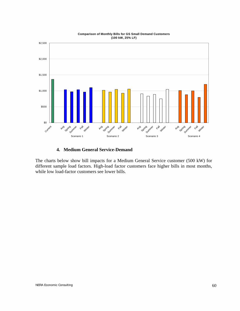
Comparison of Monthly Bills for GS Small Demand Customers (100 kW, 25% LF)
$0
$500
$1,000
$1,500
$2,000
$2,500
Curren
t A
vg
Spri
ng
Sum
mer Fall
Wint
er A
vg
Spri
ng
Sum
mer Fall
Wint
er A
vg
Spri
ng
Summer
Fall
Wint
er A
vg
Spri
ng
Sum
mer Fall
Wint
er
Scenario 1 Scenario 2 Scenario 3 Scenario 4
4. Medium General Service-Demand
The charts below show bill impacts for a Medium General Service customer (500 kW) for different sample load factors. High-load factor customers face higher bills in most months, while low load-factor customers see lower bills.
NERA Economic Consulting 60

Comparison of Monthly Bills for GS Medium Demand Customers (500 kW, 100% LF)
$0
$2,000
$4,000
$6,000
$8,000
$10,000
$12,000
$14,000
$16,000
$18,000
Curren
t A
vg
Spri
ng
Sum
mer Fall
Wint
er A
vg
Spri
ng
Sum
mer Fall
Wint
er A
vg
Spri
ng
Sum
mer Fall
Wint
er A
vg
Spri
ng
Sum
mer Fall
Wint
er
Scenario 1 Scenario 2 Scenario 3 Scenario 4
Comparison of Monthly Bills for GS Medium Demand Customers (500 kW, 75% LF)
$0
$2,000
$4,000
$6,000
$8,000
$10,000
$12,000
$14,000
$16,000
$18,000
Curren
t A
vg
Spring
Summer
Fall
Wint
er A
vg
Spring
Summer
Fall
Wint
er A
vg
Spring
Summer
Fall
Wint
er A
vg
Spring
Summer
Fall
Wint
er
Scenario 1 Scenario 2 Scenario 3 Scenario 4
NERA Economic Consulting 61

Comparison of Monthly Bills for GS Medium Demand Customers (500 kW, 50% LF)
$0
$1,000
$2,000
$3,000
$4,000
$5,000
$6,000
$7,000
$8,000
$9,000
$10,000
Curren
t A
vg
Spri
ng
Sum
mer Fall
Wint
er A
vg
Spri
ng
Sum
mer Fall
Wint
er A
vg
Spri
ng
Sum
mer Fall
Wint
er A
vg
Spri
ng
Sum
mer Fall
Wint
er
Scenario 1 Scenario 2 Scenario 3 Scenario 4
Comparison of Monthly Bills for GS Medium Demand Customers (500 kW, 25% LF)
$0
$1,000
$2,000
$3,000
$4,000
$5,000
$6,000
$7,000
$8,000
$9,000
$10,000
Curren
t A
vg
Spri
ng
Sum
mer Fall
Wint
er A
vg
Spri
ng
Sum
mer Fall
Wint
er A
vg
Spri
ng
Sum
mer Fall
Wint
er A
vg
Spri
ng
Sum
mer Fall
Wint
er
Scenario 1 Scenario 2 Scenario 3 Scenario 4
5. Large General Service-Demand
We analyzed the four different alternative rate structures for the three separate large general service groups: below 30 kV, between 30 and 100 kV and higher than 100 kV. The charts
NERA Economic Consulting 62

below show the monthly bills for selected usage under each alternative scenario. Customers with low load factors (25 and 50 percent) tend to see lower monthly bills under the four alternative scenarios. A review of the bill impacts by voltage level indicates that high-voltage customers generally see smaller bill impacts than the lower voltage levels.
Seasonal Monthly Bills for Large GS Customers (<30kV) Comparison of Monthly Bills for GS Large Demand <30 KV Customers
(5 MW, 100% LF)
$0
$20,000
$40,000
$60,000
$80,000
$100,000
$120,000
$140,000
$160,000
Curren
t A
vg
Spri
ng
Summer
Fall
Wint
er A
vg
Spri
ng
Summer
Fall
Wint
er A
vg
Spri
ng
Summer
Fall
Wint
er A
vg
Spri
ng
Summer
Fall
Wint
er
Scenario 1 Scenario 2 Scenario 3 Scenario 4
Comparison of Monthly Bills for GS Large Demand <30 KV Customers
(5 MW, 75% LF)
$0
$20,000
$40,000
$60,000
$80,000
$100,000
$120,000
$140,000
$160,000
Curren
t A
vg
Spring
Sum
mer Fall
Wint
er A
vg
Spring
Sum
mer Fall
Wint
er A
vg
Spring
Sum
mer Fall
Wint
er A
vg
Spring
Sum
mer Fall
Wint
er
Scenario 1 Scenario 2 Scenario 3 Scenario 4
NERA Economic Consulting 63

Comparison of Monthly Bills for GS Large Demand <30 KV Customers (5 MW, 50% LF)
$0
$10,000
$20,000
$30,000
$40,000
$50,000
$60,000
$70,000
$80,000
$90,000
$100,000
Curren
t A
vg
Spri
ng
Sum
mer Fall
Wint
er A
vg
Spri
ng
Sum
mer Fall
Wint
er A
vg
Spri
ng
Sum
mer Fall
Wint
er A
vg
Spri
ng
Sum
mer Fall
Wint
er
Scenario 1 Scenario 2 Scenario 3 Scenario 4
Comparison of Monthly Bills for GS Large Demand <30 KV Customers
(5 MW, 25% LF)
$0
$10,000
$20,000
$30,000
$40,000
$50,000
$60,000
$70,000
$80,000
$90,000
$100,000
Curren
t Avg
Spring
Summer
Fall
Wint
er Avg
Spring
Summer
Fall
Wint
er Avg
Spring
Summer
Fall
Wint
er Avg
Spring
Summer
Fall
Wint
er
Scenario 1 Scenario 2 Scenario 3 Scenario 4
NERA Economic Consulting 64
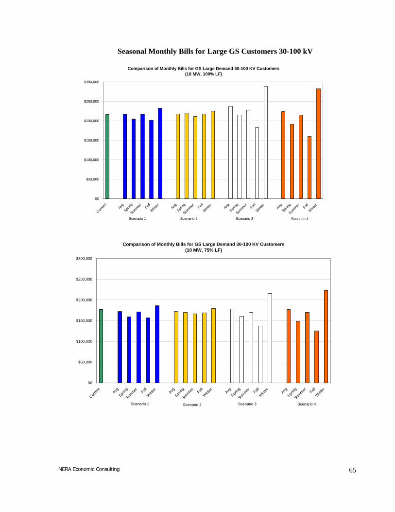
Seasonal Monthly Bills for Large GS Customers 30-100 kV
Comparison of Monthly Bills for GS Large Demand 30-100 KV Customers (10 MW, 100% LF)
$0
$50,000
$100,000
$150,000
$200,000
$250,000
$300,000
Curren
t A
vg
Spring
Sum
mer Fall
Wint
er A
vg
Spring
Sum
mer Fall
Wint
er A
vg
Spring
Sum
mer Fall
Wint
er A
vg
Spring
Sum
mer Fall
Wint
er
Scenario 1 Scenario 2 Scenario 3 Scenario 4
Comparison of Monthly Bills for GS Large Demand 30-100 KV Customers (10 MW, 75% LF)
$0
$50,000
$100,000
$150,000
$200,000
$250,000
$300,000
Curren
t A
vg
Spring
Summer
Fall
Wint
er A
vg
Spring
Summer
Fall
Wint
er A
vg
Spring
Summer
Fall
Wint
er A
vg
Spring
Summer
Fall
Wint
er
Scenario 1 Scenario 2 Scenario 3 Scenario 4
NERA Economic Consulting 65

Comparison of Monthly Bills for GS Large Demand 30-100 KV Customers (10 MW, 50% LF)
$0
$20,000
$40,000
$60,000
$80,000
$100,000
$120,000
$140,000
$160,000
$180,000
Curren
t A
vg
Spri
ng
Sum
mer Fall
Wint
er A
vg
Spri
ng
Sum
mer Fall
Wint
er A
vg
Spri
ng
Sum
mer Fall
Wint
er A
vg
Spri
ng
Sum
mer Fall
Wint
er
Scenario 1 Scenario 2 Scenario 3 Scenario 4
Comparison of Monthly Bills for GS Large Demand 30-100 KV Customers (10 MW, 25% LF)
$0
$20,000
$40,000
$60,000
$80,000
$100,000
$120,000
$140,000
$160,000
$180,000
Curren
t A
vg
Spri
ng
Sum
mer Fall
Wint
er A
vg
Spri
ng
Sum
mer Fall
Wint
er A
vg
Spri
ng
Sum
mer Fall
Wint
er A
vg
Spri
ng
Sum
mer Fall
Wint
er
Scenario 1 Scenario 2 Scenario 3 Scenario 4
NERA Economic Consulting 66

Seasonal Monthly Bills for Large GS Customers (>100 kV)
Comparison of Monthly Bills for GS Large Demand >100 KV Customers (50 MW, 100% LF)
$0
$200,000
$400,000
$600,000
$800,000
$1,000,000
$1,200,000
$1,400,000
Curren
t A
vg
Spri
ng
Sum
mer Fall
Wint
er A
vg
Spri
ng
Sum
mer Fall
Wint
er A
vg
Spri
ng
Sum
mer Fall
Wint
er A
vg
Spri
ng
Sum
mer Fall
Wint
er
Scenario 1 Scenario 2 Scenario 3 Scenario 4
Comparison of Monthly Bills for GS Large Demand >100 KV Customers (50 MW, 75% LF)
$0
$200,000
$400,000
$600,000
$800,000
$1,000,000
$1,200,000
$1,400,000
Curren
t Avg
Spri
ng
Summer
Fall
Wint
er Avg
Spri
ng
Summer
Fall
Wint
er Avg
Spri
ng
Summer
Fall
Wint
er Avg
Spri
ng
Summer
Fall
Wint
er
Scenario 1 Scenario 2 Scenario 3 Scenario 4
NERA Economic Consulting 67

Comparison of Monthly Bills for GS Large Demand >100 KV Customers (50 MW, 50% LF)
$0
$100,000
$200,000
$300,000
$400,000
$500,000
$600,000
$700,000
$800,000
Curren
t A
vg
Spri
ng
Sum
mer Fall
Wint
er A
vg
Spri
ng
Sum
mer Fall
Wint
er A
vg
Spri
ng
Sum
mer Fall
Wint
er A
vg
Spri
ng
Sum
mer Fall
Wint
er
Scenario 1 Scenario 2 Scenario 3 Scenario 4
Comparison of Monthly Bills for GS Large Demand >100 KV Customers (50 MW, 25% LF)
$0
$100,000
$200,000
$300,000
$400,000
$500,000
$600,000
$700,000
$800,000
Curren
t A
vg
Spring
Summer
Fall
Wint
er Avg
Spring
Summer
Fall
Wint
er Avg
Spring
Summer
Fall
Wint
er A
vg
Spri
ng
Summer
Fall
Wint
er
Scenario 1 Scenario 2 Scenario 3 Scenario 4
NERA Economic Consulting 68

VIII. CONCLUSIONS AND RECOMMENDATIONS
The results of the analysis undertaken for this report suggest that, unless implementation costs are unexpectedly high, there is potential for progress toward achieving many of Manitoba’s electricity rate objectives by adoption of inverted and/or TOD rate structures.
Based on (1) the specific illustrative rates developed for this study, which are necessarily constrained by the need to avoid drastic bill impacts and other rate objectives in Manitoba, (2) estimated marginal costs and (3) the assumed elasticities, the structures for each class that offer the highest potential cost savings for the utility are as follows:
Residential Scenario 1 and Scenario 2 create similar savings
GSS-ND Scenario 1 – 75% CBL block with seasonal energy charges
GSS-D Scenario 2 – 90% CBL block with demand and TOD energy charges
GSM Scenario 2 – 90% CBL block with demand and TOD energy charges; slightly lower savings with Scenario 1- 90% CBL with demand and seasonal energy charges
GSL <30 kV Scenario 2 - 90% CBL block with demand and TOD energy charges
GSL 30-100 kV Scenarios 1 and 2 create virtually the same savings
GSL >100 kV Scenarios 1 and 2 create virtually the same savings The illustrative rates with the largest welfare gains, which take into account not only utility cost savings but also effects on consumer surplus and reductions in wasted resources, for each class are as follows:
Residential Scenario 2 – single set of seasonal first blocks for all customers
GSS-ND Scenario 2 – unblocked seasonal and TOD energy charges
GSS-D, GSM, GSL (All demand-metered)
Scenario 2 – 90% CBL block with demand and TOD energy charges
The bill impacts for given levels of consumption shown in Section VII.D suggest that most of the scenarios will produce bill impacts that are acceptable. However, because a given customer (particularly residential and GSS-ND) may use quite different amounts of electricity from season to season, the overall effect on particular customer types should be evaluated before a new rate structure proposal is implemented.
Specific observations can be summarized as follows:
NERA Economic Consulting 69

• Preferred Structures
1. Manitoba Hydro’s marginal costs vary by season and TOD and, therefore, time-differentiated rates improve efficiency and equity. The preliminary results support increase in net welfare. Seasonal plus diurnal price differences generally produce the best results, when TOD metering is cost-effective and customer understanding is not a problem.
2. Inverted rates improve efficiency over unblocked or declining block rates, particularly when run-off rates are seasonally differentiated. Seasonal inverted block rates can be more efficient than unblocked TOD rates in cases where a large difference between class revenue requirement and marginal cost revenues require large differences between TOD charges and marginal costs.
• Residential customers
3. A rate structure with the same first block for all residential customers produced higher welfare gains in the tests conducted in this review, and is likely to be more feasible than inverted blocks with a first block size that depends upon space heating type. There is an equity argument that customers who have no alternative to electric space because there is no gas service in their area (or it is prohibitively expensive to convert to gas46) should have a larger first block than customers with access to gas. However, this approach creates significant administrative problems in determining which customers qualify for the larger first block.
4. Customers with electric space heat capability are typically more elastic than those without, which implies that it is more important for them to face a marginal-cost based price signal in the heating season. This suggests that the first block size in an inverted block rate structure should be set low enough to put most customers with electric heat into the more efficient, marginal cost-based second block.
• General Service customers
5. The tested rate structures with both demand and TOD energy charges tended to produce larger welfare gains than those without demand charges. (Although this may be an artifact of the particular charges in the tested rates and the assumed elasticities.)
6. For equity and competitive reasons, inverted block structures for General Service customers should ideally define the first block in terms of a percent of CBL, although this will introduce significant rate administration costs. Putting all 63,000 GS customers on rates with CBLs would be administratively onerous.
46 Retrofit is estimated to cost $5,000-$7,000.
NERA Economic Consulting 70

Such a rate structure might be feasible for GSL and perhaps GSM customers. A possible solution for this problem would be to offer GSS-ND customers a choice between (a) a fixed first block inverted kWh block structure and (b) TOU (non-blocked) energy charges. To prevent revenue erosion as customers choose the most advantageous rate, Manitoba Hydro would need to forecast customers’ choices.
7. Inverted block structures with a fixed first block size for general service customers create inequities within the class and distort the competitive position of businesses. Only three of the utilities in our survey have inverted block kWh charges for small and medium non-residential customers.
IX. NEXT STEPS
This report points to new rate structures that have the potential to provide important benefits for Manitoba. However, the results from the rate structures tested are based on explicit assumptions about factors such as marginal costs, elasticity effects, and changes in authorized class revenue requirements. Furthermore, the effects quantified apply to the specific rates tested, and not to all rates with similar structures. It is important to keep in mind that any specific new rate structure proposed for implementation in Manitoba should be studied in much more detail to quantify implementation costs, identify effects on Manitoba Hydro’s cash flow and financial risk, and to determine the likely effects on a wide range of customer types and sizes.
Maximizing simplicity and customer acceptance might require simpler rate structures; e.g., two seasonal pricing periods instead of four. However, simplification involves some sacrifice of efficient price signals. For example, averaging costs to create two seasons instead of four mutes the price signal in the high-cost months. With any change in rate structure, carefully designed programs that inform customers of the coming changes and how they can adapt to them are important. Gradual implementation of new structures (and other transition mechanisms) may also be appropriate. Customers with unusual load patterns may be particularly adversely affected by a change of rate structure. A temporary “bill limiter” mechanism that limits the percentage change in their bill (compared to current rates) and gradually increases the limit is one way to ease the transition for outliers, while improving price signals for most customers.
NERA Economic Consulting 71

APPENDIX A. SURVEY ELECTRICITY RATE STRUCTURES IN NORTH AMERICA
Residential Rates
Utility Rate Energy (kWh) Demand (kW) kWh Charge
Structure kWh Blocks TD kW
Structure kW
Blocks TD
Avista 1 -Residential
INVERTED, 3 kWh blocks
First: 600 kWh/mo (4.77c), Next 700 kWh/mo (5.72c); Third: >1300kWh/mo (6.87c)
No TOU NA NA NA
11-12 Resid and Farm GS
No block charge NA No TOU INVERTED, 2 blocks
First: < 20kW, zero
charge
NA
BC Hydro Residential 1101, 1111, 1121. Zone I
No block charge NA No TOU NA NA NA
Residential 1107, 1117, 1127. Zone II
INVERTED, 2 blocks
First: 3,000kWh per 2-mo (6.19c/kWh); > 3,000kWh/2mo. (10.63c/kWh)
No TOU NA NA NA
Multi-Residential 1131, 1133. Zone I
3 blocks; same charge for blocks 1
and 3, higher charge for block2.
First 400 kWh/2 mo (6.16c/kWh); Next 200 kWh (6.96c); > 600 kWh (6.16c)
No TOU NA NA NA
Multi-Residential1132, 1134 Zone II
INVERTED, 3 blocks
6.16c/kWh for first 400 kWh per 2 mo, 6.96c/kWh for next 200 kWh, 10.63c/kWh for the rest.
No TOU NA NA NA
Hydro Quebec D-Residential
INVERTED, 2 blocks
First 30 kWh/day (4.95c/kWh), all over (6.24c/kWh)
No TOU INVERTED, 2 blocks
zero charge for <50kW, $3.21/kW for rest the winter
Winter (Dec-Mar); Summer (rest)
DT- Residential Dual Energy
RTP (temperature-triggered)
NA Warm (> -12C or -15C) by zone: 3.62 c/kWh; Cold (< -12C or -15C): 16.24c/kWh
NA NA NA
DM - Residential - Multi-Dwelling
INVERTED, 2 blocks
First 30 kWh/day * multiplier reflecting # of dwelling units 4.95c/kWh, all over: 6.24c/kWh)
No TOU INVERTED, 2 blocks
Zero charge for <50kW, $0.81 per excess kW
Winter (Dec-Mar)
NERA Economic Consulting 72

Residential Rates
Utility Rate
Energy (kWh) Demand (kW) kWh Charge
Structure kWh Blocks TD kW kW
Blocks Structure TD
DH -Residential experimental TOU (optional)
TOD, no-block charge
NA peak and off-peak prices in winter; all summer is off-peak
NA NA NA
Hydro One Residential INVERTED, 2 blocks, for supply
component; Flat for T&D
Blocks: <750kWh (4.70c), >750 kWh (5.50c)
No TOU NA NA NA
Idaho Power Residential INVERTED, 2 blocks (summer
only)
Flat charge in winter. Two-block inverted rate in summer kWh >300kWh
Summer (June 1-Aug 31)
NA NA NA
Newfoundland and Labrador Hydro
Domestic No block charge NA no TOU NA NA NA
Domestic Diesel
INVERTED, 3 blocks
First 700 kWh/mo, next 300 kWh, rest
no TOU NA NA NA
Northern States Power
A01 Residential
No-block, seasonal; lower winter rate for space heating customers
NA Summer (June-Sep)
NA NA NA
A02 Optional Residential TOD
No-block;TOD; lower winter peak charge for space heating custs.
NA Summer (June-Sep)
NA NA NA
Pacificorp - OR 4 -Standard Residential
INVERTED, 3 blocks
<500, 501-1000 and >1000kWh
no TOU NA NA NA
4 -TOU Residential Optional
TOD, no-block charge
NA On and off-peak hours. Higher summer charges (Apr-Oct)
NA NA NA
Pacificorp - WA
16 -Residential
INVERTED, 2 blocks
1st block = 600 kWh/mo.
no TOU NA NA NA
17- Low-income residential
INVERTED, 2 blocks
declining block if 100% of pov line or less; slight invert. block if 101-125% of pov. line
no TOU NA NA NA
Portland General Electric
7 -Residential (standard)
INVERTED, 2 blocks
Slight inversion (4.3c for first 250, 4.8c for rest)
no TOU NA NA NA
7 -Residential (optional TOU)
INVERTED (Credit for first 250 kWh),
TOD
Credit of 0.48c/kWh for 1st 250 kWh
3 TOD periods
NA NA NA
Puget Sound 7 -Residential
INVERTED, 2 blocks
<600kWh (6.28c/kWh); >600kWh (7.92 c/kWh)
No TOU NA NA NA
Seattle City Light
RSC, RSS - Residential (City and Suburban)
INVERTED, 3 blocks
Three (highly) inverted seasonal blocks. First two blocks longer in the winter, but charges are the same.
Winter (Oct-Mar)
NA NA NA
NERA Economic Consulting 73
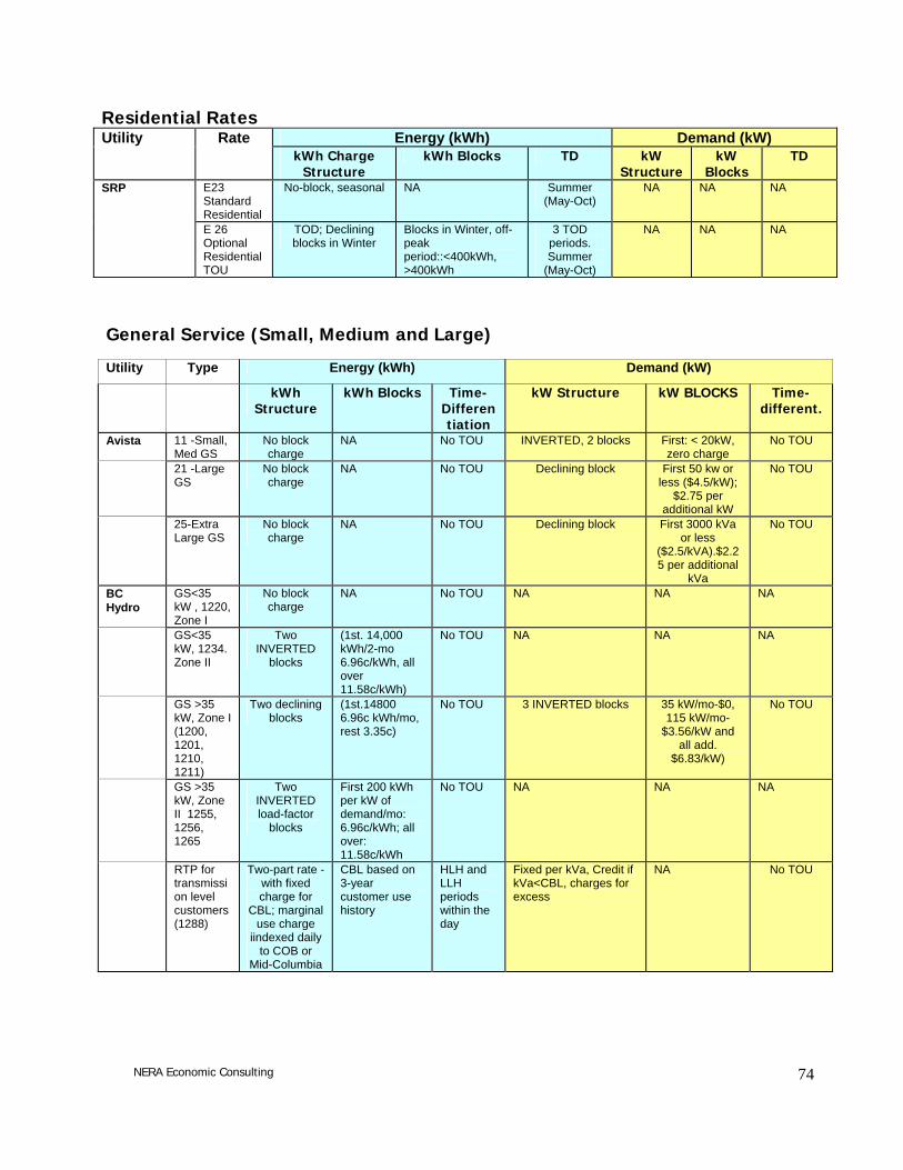
Residential Rates
Utility Rate
Energy (kWh) Demand (kW) kWh Charge
Structure kWh Blocks TD kW kW
Blocks Structure TD
SRP E23 Standard Residential
No-block, seasonal NA Summer (May-Oct)
NA NA NA
E 26 Optional Residential TOU
TOD; Declining blocks in Winter
Blocks in Winter, off-peak period::<400kWh, >400kWh
3 TOD periods. Summer
(May-Oct)
NA NA NA
General Service (Small, Medium and Large)
Utility Type Energy (kWh) Demand (kW)
kWh Structure
kWh Blocks Time-Differentiation
kW Structure kW BLOCKS Time-different.
Avista 11 -Small, Med GS
No block charge
NA No TOU INVERTED, 2 blocks First: < 20kW, zero charge
No TOU
21 -Large GS
No block charge
NA No TOU Declining block First 50 kw or less ($4.5/kW);
$2.75 per additional kW
No TOU
25-Extra Large GS
No block charge
NA No TOU Declining block First 3000 kVa or less
($2.5/kVA).$2.25 per additional
kVa
No TOU
BC Hydro
GS<35 kW , 1220, Zone I
No block charge
NA No TOU NA NA NA
GS<35 kW, 1234. Zone II
Two INVERTED
blocks
(1st. 14,000 kWh/2-mo 6.96c/kWh, all over 11.58c/kWh)
No TOU NA NA NA
GS >35 kW, Zone I (1200, 1201, 1210, 1211)
Two declining blocks
(1st.14800 6.96c kWh/mo, rest 3.35c)
No TOU 3 INVERTED blocks 35 kW/mo-$0, 115 kW/mo-
$3.56/kW and all add.
$6.83/kW)
No TOU
GS >35 kW, Zone II 1255, 1256, 1265
Two INVERTED load-factor
blocks
First 200 kWh per kW of demand/mo: 6.96c/kWh; all over: 11.58c/kWh
No TOU NA NA NA
RTP for transmission level customers (1288)
Two-part rate - with fixed charge for
CBL; marginal use charge
iindexed daily to COB or
Mid-Columbia
CBL based on 3-year customer use history
HLH and LLH periods within the day
Fixed per kVa, Credit if kVa<CBL, charges for excess
NA No TOU
NERA Economic Consulting 74

General Service (Small, Medium and Large)
Utility Type Energy (kWh) Demand (kW)
kWh Structure
kWh Blocks Time-Differentiation
kW Structure kW BLOCKS Time-different.
Hydro Quebec
G Small-Power Business <100kW
Two declining blocks
First 30 kWh/day (4.95c/kWh), all over (6.24c/kWh)
No TOU INVERTED, 2 blocks $14.19/kW above 40 kW;
min. billing demand is 65% of peak winter.
Winter (Dec-Mar); Summer (rest)
Small and Medium Business (G9 & M9)
No block, flat charge
NA No TOU No-block demand charge
NA No TOU
M - Medium-Power Business >100kW, <5000kW
Two declining blocks
No TOU No-block demand charge and additional (higher) charge for excess kW in the winter (above 110% of CD)
NA Winter (Dec-Mar)
MR - Optional RTP for Medium (pilot)
Two-part rate - declining two block charge
for CBL, hourly charge for marginal
use
NA Summer/Winter for CBL; Hourly prices for surplus energy
No-block demand charge and additional (higher) charge for excess kW in the winter (above 110% of CD)
NA Winter (Dec-Mar)
LR- Optional RTP (>5000kW)
Two-part rate - declining two block charges for CBL use, hourly charge for marginal
use
NA Summer/Winter for CBL; Hourly prices for surplus energy
No-block demand charge and additional (higher) charge for excess kW in the winter (above 110% of CD)
NA Winter (Dec-Mar)
L -Large Power >5000kW
No-block charge
NA No TOU No-block demand charge and additional (higher) charge for excess kW in the winter (above 110% of CD)
NA Winter (Dec-Mar)
LC Large Power - intermittent variable price
No-block, customer's bid
price
NA Seasonal NA NA NA
LP -Large Power – intermittent, fixed price
Winter - no block charge;
summer INVERTED load-factor
charges
Load-factor blocks: 3.79c per 300 hours of use; 7.62 cents for rest
Seasonal NA NA NA
Hydro One
Small Business (<50kW)
INVERTED, 2 blocks for
supply component; Flat for T&D
Blocks: <750kWh, >750 kWh
No TOU NA NA NA
Med Business (>50 kW)
INVERTED, 2 blocks for
supply component; Flat for T&D
Blocks: <750kWh, >750 kWh
No TOU D &T kW charge, no block
NA No TOU
NERA Economic Consulting 75

General Service (Small, Medium and Large)
Utility Type Energy (kWh) Demand (kW)
kWh Structure
kWh Blocks Time-Differentiation
kW Structure kW BLOCKS Time-different.
Idaho Power
Small Commercial
No-block charge in
winter. Two INVERTED
blocks in summer
Summer blocks: <300, >300kWh
Summer (June 1-Aug 31)
NA NA NA
Large Commercial
No-block, seasonal charges.
NA Summer (June 1-Aug 31)
No-block seasonal charges (Higher in summer)
NA Summer (June 1-Aug 31)
Large GS (>3000 kWh/mo)
No-block; seasonal charges.
NA Summer (June 1-Aug 31)
Seasonal charge per kW of max demand and per kW of basic load capacity (avg of 2 highest months in last 12 months)
NA Summer (June 1-Aug 31)
Small GS 0-10 kW
No-block charge
NA no TOU NA NA NA
Small GS 10-100 kW
No-block charge
NA no TOU No-block charge NA No TOU
NFL
GS > 110kVA
No-block charge
NA no TOU No-block charge NA No TOU
Industrial No-block charge
NA no TOU No-block charge NA No TOU
GS 10-100 kW (110 kVa)
Two declining load-factor
blocks
First 150 kWh per kW/mo, rest.
no TOU Seasonal, no-block charge.
NA Winter (Dec-Mar)
GS 110 kVa -1000 kVA
Two declining load-factor
blocks
First 150 kWh per kW/mo, up to 30 MWh/mo., rest of kWh.
no TOU Seasonal, no block charge.
NA Winter (Dec-Mar)
GS >1000 kVA
Two declining kWh blocks
First 150,000 kWh, rest
no TOU Seasonal, no block charge.
NA Winter (Dec-Mar)
GS Diesel Two INVERTED kWh-blocks
First 700 kWh, rest
no TOU NA NA NA
Northern States Power
Small GS A10
No block, seasonal charges
NA Seasonal; Summer (June-Sep)
NA NA NA
Small GS Time of Day A12&A18
No block, seasonal and TOD charges
NA Summer (June-
Sep) and TOD
NA NA NA
GS - A14 Declining load-factor block Seasonal No block charge NA Seasonal
General Time of Day Service A15
Declining load-factor
block on and off-peak charges
(run-off block not to exceed 50% of total kWh)
Seasonal and TOD
No block charge NA Seasonal & TOD
RTP (A62,A63)
Day-type, TOD charges
NA Seasonal and TOD
No-block per kW of contract demand charge
NA No TOU
Pacificorp - OR Two declining blocks
no TOU Two quasi-inverted charges:
Zero charge for <15 kW
no TOU
NERA Economic Consulting 76

General Service (Small, Medium and Large)
Utility Type Energy (kWh) Demand (kW)
kWh Structure
kWh Blocks Time-Differentiation
kW Structure kW BLOCKS Time-different.
23-TOU GS Small Optional
Rate 23 with on-peak
surcharge & off-peak
credit. Higher summer
surcharge.
NA Summer (Apr-Oct)
Two quasi inverted charges:
Zero charge for <15 kW
no TOU
28- GS Large 31-200 kW
Two declining blocks
no TOU Four declining block load-size charge; no-block demand charge
no TOU
30 -GS Large 200-999 kW
Two declining blocks
no TOU Two declining block load-size charge; flat demand charge
no TOU
48 -Large GS >1000 kW
No-block energy charge
NA no TOU No-block demand charge
NA no TOU
PacificorWA
24 -General Service
Three declining energy blocks no TOU Declining two- block basic charge (average of 2 highest monthly peak demands in 12 months). INVERTED block demand charges (highest 15 min demand).
First 15 kW, rest no TOU
36- Large GS - Optional <1000 kW
Two declining energy blocks Declining three-block charges (average of 2 highest peak demands in 12 months). Flat max demand charge (highest 15 min kW).
First 100kW, next 200kW, rest (for basic charge)
no TOU
48T-Large GS - TOU >1000 kW
No-block TOD charge
NA 3 TOD periods
Two-block declining basic charge. On-peak demand charge
Peak period
Portland General Electric
32-Small non-resid SOS (non-TOU)
Declining blocks for distribution charge
no TOU NA NA NA
32-Small non-resid SOS (opt-TOU)
Declining blocks for distribution charge
3 TOD periods
NA NA NA
38-Large non-res SOS (opt TOD)
TOD no-block charge
NA 3 TOD periods
NA NA NA
83-Lrg GS with facil. Capacity>1MW
No block, TOD charges
NA TOD (peak and off-peak) prices change monthly
Secondary delivery has INVERTED block kW charges per kW.
First 30 kW, over 30 kW
no TOU
87Experimental RTP for non-res >1MW
CBL +or- RTP CBL, marginal kWh
Hourly NA NA NA
Puget Sound
25-Small Dmd GS
Two declining kWh blocks. Winter (Oct-Mar)
Seasonal INVERTED charge per kW.
First 50 kW are free.
Winter (Oct-Mar)
NERA Economic Consulting 77

General Service (Small, Medium and Large)
Utility Type Energy (kWh) Demand (kW)
kWh Structure
kWh Blocks Time-Differentiation
kW Structure kW BLOCKS Time-different.
26-Large Dmd GS
No block, seasonal charges.
NA Winter (Oct-Mar)
Seasonal no-block charge. Higher winter charge
NA Winter (Oct-Mar)
43-Limited Interruptible (Primary)
No block, seasonal charges.
NA Winter (Oct-Mar)
No-block charge (per kW) plus per kW of critical.
NA Winter (Oct-Mar)
46-HV Interruptible
No block, seasonal charges.
NA Winter (Oct-Mar)
No-block charge (per kVa)
NA Winter (Oct-Mar)
49-HV GS No block, seasonal charges.
NA Winter (Oct-Mar)
No-block charge (per kVa)
NA Winter (Oct-Mar)
Seattle City Light
Small GS (SMC; SMS)
No block charge
NA no TOU NA NA NA
Medium GS -
No block charge
NA no TOU No-block charge NA no TOU
Large GS City
No block, TOD charges
NA Peak and off-peak (no seasonal)
No-block, TOD kW charges
NA Peak /off-peak (no seasonal)
Large Network GS
No block, TOD charges
NA Peak and off-peak (no seasonal)
No-block, TOD kW charges
NA Peak /off-peak (no seasonal)
Large GS Suburban
No block, TOD charges
NA Peak and off-peak (no seasonal)
No-block, TOD kW charges
NA Peak /off-peak (no seasonal)
High-demand GS City
No block, TOD charges
NA Peak and off-peak (no seasonal)
No-block, TOD kW charges
NA Peak /off-peak (no seasonal)
High Demand Variable GS (optional)
TOD kWh charges
(indexed daily to COB or
Mid-Columbia)
NA Peak and off-peak; daily variation.
No-block, TOD kW charges
NA Peak /off-peak (no seasonal)
SRP 32 -Optional TOU GS
No-block; TOU charges
NA Summer (May-Oct);
3 TOD periods
No block TOU charge NA Seasonal & TOD
36- Standard GS
Declining load-factor blocks in
Winter; no block in summer
Blocks in Winter, off-peak period:<400kWh, >400kWh
Summer (May-Oct)
INVERTED, 2 blocks First 5 kW free Seasonal
61 -Secondary Large GS >300,000 kWh/mo
No-block; TOD charges
NA Summer (May-Oct);
3 TOD periods
No block; Facilities Charge per kW (15-mo.
ratchet)
NA no TOU
NERA Economic Consulting 78

General Service (Small, Medium and Large)
Utility Type Energy (kWh) Demand (kW)
kWh Structure
kWh Blocks Time-Differentiation
kW Structure kW BLOCKS Time-different.
63-Primary Large GS >300,000 kWh/mo
No-block; TOD charges
NA Summer (May-Oct);
3 TOD periods
No block; Facilities Charge per kW (15-mo.
ratchet)
NA no TOU
Note: Hydro One only serves to residential, farm and small and med business. Large customers (annual usage above 250 MWh) face hourly spot market prices, buying directly from the real-time market.
NERA Economic Consulting 79

APPENDIX B. MANITOBA HYDRO CURRENT RATES (APRIL 1, 2005)
(Note: Bill calculations shown earlier in report were based on rates effective August 1, 2004)
Residential
Monthly Basic Charge:
NOT Exceeding 200 Amp $6.25
Exceeding 200 Amp $12.50
Plus
Energy Charge:
First 175 kW.h @ 5.780¢ /kW.h
Balance of kW.h @ 5.654¢ /kW.h
General Service Small (Non-Residential; Utility-owned Transformation NOT exceeding 200 kV.A) Tariff No. 2005-20 and 2005-21
Monthly Basic Charge (for Single Phase cust): $15.86
Monthly Basic Charge (for Three-Phase cust): $22.01
Plus Energy Charge:
First 11,090 kW.h @ 6.004¢ /kW.h
Next 8,500 kW.h @* 3.936¢ /kW.h Balance of kW.h @ 2.444¢ /kW.h
Plus Demand Charge: First 50 kV.A of Monthly Recorded Demand @ No Charge
Balance of Recorded Demand @ $8.32 /kV.A
NERA Economic Consulting 80

Notes: Minimum monthly bill is the Basic Charge plus Demand Charge. Primary metering of multiple Utility-owned transformation - add 2% to kV.A for each transformation greater than one.
* Demand Charge is applied to the Monthly Billing Demand defined as the greater of the following expressed in kV.A:
i. measured demand.
ii. 70% of highest measured demand in the Billing Year for the months of December, January, February.
iii. 25% of contract demand.
iv. 25% of the highest measured demand in any of the previous 12 months.
General Service Medium (Non-Residential; Utility-owned Transformation exceeding 200 kV.A) Tariff No. 2005-30 Monthly Basic Charge: $27.65
Plus Energy Charge: 2.444¢ /kW.h
Plus Demand Charge*: $8.32 /kV.A Notes: Minimum monthly bill is the Basic Charge plus Demand Charge. Primary metering of multiple Utility-owned transformation - add 2% to kV.A for each transformation greater than one.
* Demand Charge is applied to the Monthly Billing Demand defined as the greater of the following expressed in kV.A:
i. measured demand.
ii. 70% of highest measured demand in the Billing Year for the months of December, January, February.
iii. 25% of contract demand.
iv. 25% of the highest measured demand in any of the previous 12 months.
NERA Economic Consulting 81

General Service Large
(Non-Residential; Customer-owned Transformation)
Exceeding 750 V but NOT exceeding 30 kV Tariff No. 2005-60 Energy Charge: 2.284¢ /kW.h
Plus Demand Charge*: $7.09 /kV.A
Exceeding 30 kV but NOT exceeding 100 kV Tariff No. 2005-61 Energy Charge: 2.215¢ /kW.h
Plus Demand Charge*: $6.05 /kV.A
Exceeding 100 kV Tariff No. 2005-62 Energy Charge: 2.187¢ /kW.h
Plus Demand Charge*: $5.40 /kV.A
Notes: Minimum monthly bill is the Demand Charge.
*Demand Charge is applied to the Monthly Billing Demand defined as the greater of the following expressed in kV.A:
i. measured demand.
ii. 70% of highest measured demand in the Billing Year for the months of December, January, February.
iii. 25% of contract demand.
iv. 25% of the highest measured demand in any of the previous 12 months.
NERA Economic Consulting 82

APPENDIX C. ILLUSTRATIVE RATES AND AVERAGE MONTHLY BILL COMPARISONS
Scenario 1: Residential Standard
Illustrative Rates
Basic Charge: $6.25
Energy Charge:
First Block kWh
1st Block Rate
Run-Off Rate
Spring 600 3.756 5.0 Summer 600 3.756 5.2 Fall 600 3.756 5.0 Winter 600 3.756 9.0
Changes in Average Monthly Bill
Average Monthly Bill Consumption Current Illustrative Difference Percent kWh/month Cdn$/month Cdn$/month Cdn$/month Change
250 $20.49 $15.64 ($4.85) -23.67% 500 $34.23 $25.03 ($9.20) -26.88% 750 $47.97 $38.39 ($9.58) -19.98%
1000 $61.71 $54.39 ($7.32) -11.87% 2000 $116.67 $118.39 $1.72 1.47% 5000 $281.55 $310.39 $28.84 10.24%
Average Spring and Fall Monthly Bill 250 $20.49 $15.64 ($4.85) -23.67% 500 $34.23 $25.03 ($9.20) -26.88% 750 $47.97 $36.29 ($11.68) -24.36%
1000 $61.71 $48.79 ($12.92) -20.94% 2000 $116.67 $98.79 ($17.88) -15.33% 5000 $281.55 $248.79 ($32.76) -11.64%
Average Summer Monthly Bill 250 $20.49 $15.64 ($4.85) -23.67% 500 $34.23 $25.03 ($9.20) -26.88% 750 $47.97 $36.59 ($11.38) -23.73%
1000 $61.71 $49.59 ($12.12) -19.65% 2000 $116.67 $101.59 ($15.08) -12.93% 5000 $281.55 $257.59 ($23.96) -8.51%
NERA Economic Consulting 83

Average Winter Monthly Bill Consumption Current Illustrative Difference Percent kWh/month Cdn$/month Cdn$/month Cdn$/month Change
250 $20.49 $15.64 ($4.85) -23.67% 500 $34.23 $25.03 ($9.20) -26.88% 750 $47.97 $42.29 ($5.68) -11.85%
1000 $61.71 $64.79 $3.08 4.98% 2000 $116.67 $154.79 $38.12 32.67% 5000 $281.55 $424.79 $143.24 50.87%
Scenario 1: Residential All-Electric
Illustrative Rates
Basic Charge: $6.25
Energy Charge:
1st Block kWh
1st Block Rate
Run-Off Rate
Spring 1000 3.756 5.0 Summer 600 3.756 5.2 Fall 1000 3.756 5.0 Winter 1500 3.756 9.0
Changes in Average Monthly Bill
Average Monthly Bill
Consumption Current Illustrative Difference Percent kWh/month Cdn$/month Cdn$/month Cdn$/month Change
250 $20.49 $15.64 ($4.85) -23.67% 500 $34.23 $25.03 ($9.20) -26.88% 750 $47.97 $35.14 ($12.83) -26.74%
1000 $61.71 $45.74 ($15.97) -25.89% 2000 $116.67 $101.00 ($15.67) -13.44% 5000 $281.55 $293.00 $11.45 4.07%
Average Spring & Fall Monthly Bill 250 $20.49 $15.64 ($4.85) -23.67% 500 $34.23 $25.03 ($9.20) -26.88% 750 $47.97 $34.42 ($13.55) -28.25%
1000 $61.71 $43.81 ($17.90) -29.01% 2000 $116.67 $93.81 ($22.86) -19.59% 5000 $281.55 $243.81 ($37.74) -13.40%
NERA Economic Consulting 84

Average Summer Bill Consumption Current Illustrative Difference Percent kWh/month Cdn$/month Cdn$/month Cdn$/month Change
250 $20.49 $15.64 ($4.85) -23.67% 500 $34.23 $25.03 ($9.20) -26.88% 750 $47.97 $36.59 ($11.38) -23.73%
1000 $61.71 $49.59 ($12.12) -19.65% 2000 $116.67 $101.59 ($15.08) -12.93% 5000 $281.55 $257.59 ($23.96) -8.51%
Average Winter Bill 250 $20.49 $15.64 ($4.85) -23.67% 500 $34.23 $25.03 ($9.20) -26.88% 750 $47.97 $34.42 ($13.55) -28.25%
1000 $61.71 $43.81 ($17.90) -29.01% 2000 $116.67 $107.59 ($9.08) -7.78% 5000 $281.55 $377.59 $96.04 34.11%
Scenario 2: Residential Combined
Illustrative Rates
Basic Charge: $6.25
Energy Charge:
1st Block kWh
1st Block Rate
Run-Off Rate
Spring 800 3.756 5.0 Summer 600 3.756 5.2 Fall 800 3.756 5.0 Winter 1000 3.756 9.0
Changes in Average Monthly Bill
Average Monthly Bill
Consumption Current Illustrative Difference Percent kWh/month Cdn$/month Cdn$/month Cdn$/month Change
250 $20.49 $15.64 ($4.85) -23.67% 500 $34.23 $25.03 ($9.20) -26.88% 750 $47.97 $34.42 ($13.55) -28.25%
1000 $61.71 $45.60 ($16.11) -26.10% 2000 $116.67 $110.43 ($6.24) -5.35% 5000 $281.55 $299.93 $18.38 6.53%
NERA Economic Consulting 85

Average Monthly Spring & Fall Bill Consumption Current Illustrative Difference Percent kWh/month Cdn$/month Cdn$/month Cdn$/month Change
250 $20.49 $15.64 ($4.85) -23.67% 500 $34.23 $25.03 ($9.20) -26.88% 750 $47.97 $34.42 ($13.55) -28.25%
1000 $61.71 $46.30 ($15.41) -24.97% 2000 $116.67 $98.79 ($17.88) -15.33% 5000 $281.55 $248.79 ($32.76) -11.64%
Average Monthly Summer Bill 250 $20.49 $15.64 ($4.85) -23.67% 500 $34.23 $25.03 ($9.20) -26.88% 750 $47.97 $34.42 ($13.55) -28.25%
1000 $61.71 $46.70 ($15.01) -24.33% 2000 $116.67 $98.70 ($17.97) -15.40% 5000 $281.55 $254.70 ($26.85) -9.54%
Average Monthly Winter Bill 250 $20.49 $15.64 ($4.85) -23.67% 500 $34.23 $25.03 ($9.20) -26.88% 750 $47.97 $34.42 ($13.55) -28.25%
1000 $61.71 $43.81 ($17.90) -29.01% 2000 $116.67 $133.81 $17.14 14.69% 5000 $281.55 $396.30 $114.75 40.76%
NERA Economic Consulting 86

Scenario 1: Small GS Non-Demand
Illustrative Rates
CBL charge Run-off charge (cents/kWh) (cents/kWh) Spring 5.647 5.647 Summer 5.647 5.647 Fall 5.647 5.647 Winter 5.647 9.000
Notes: 1st block is 75% of CBL
Changes in Average Monthly Bill
Average Monthly Bill Consumption Current Illustrative Difference Percent kWh/month Cdn$/month Cdn$/month Cdn$/month Change
750 $59.70 $60.20 $0.50 0.83% 2000 $132.95 $134.28 $1.33 1.00% 5000 $308.75 $312.07 $3.32 1.08%
10000 $601.75 $608.39 $6.64 1.10% Average Spring/ Summer/Fall Monthly Bill
750 $59.70 $58.10 ($1.60) -2.68% 2000 $132.95 $128.69 ($4.26) -3.20% 5000 $308.75 $298.10 ($10.65) -3.45%
10000 $601.75 $580.45 ($21.30) -3.54% Average Winter Monthly Bill
750 $59.70 $64.39 $4.69 7.85% 2000 $132.95 $145.46 $12.51 9.41% 5000 $308.75 $340.01 $31.26 10.13%
10000 $601.75 $664.28 $62.53 10.39%
NERA Economic Consulting 87

Scenario 2: Small GS Non-Demand
Illustrative Rates
Energy Charges (cents/kWh)
Peak Shoulder Off-Peak Spring 4.85 3.80 2.45 Summer 6.65 4.04 1.89 Fall 4.39 3.22 2.26 Winter 23.17 3.98 3.04
Changes in Average Monthly Bill
Average Monthly Bill
Consumption Current Illustrative Difference Percent kWh/month Cdn$/month Cdn$/month Cdn$/month Change
750 $59.70 $56.89 ($2.81) -4.71% 2000 $132.95 $125.45 ($7.50) -5.64% 5000 $308.75 $290.01 ($18.74) -6.07%
10000 $601.75 $564.27 ($37.48) -6.23%
Average Spring Monthly Bill Consumption Current Illustrative Difference Percent kWh/month Cdn$/month Cdn$/month Cdn$/month Change
750 $59.70 $43.59 ($16.11) -26.99% 2000 $132.95 $89.98 ($42.97) -32.32% 5000 $308.75 $201.32 ($107.43) -34.80%
10000 $601.75 $386.89 ($214.87) -35.71% Average Summer Monthly Bill
750 $59.70 $47.89 ($11.81) -19.78% 2000 $132.95 $101.46 ($31.49) -23.68% 5000 $308.75 $230.03 ($78.72) -25.50%
10000 $601.75 $444.32 ($157.44) -26.16% Average Fall Monthly Bill
750 $59.70 $40.12 ($19.58) -32.79% 2000 $132.95 $80.75 ($52.20) -39.27% 5000 $308.75 $178.24 ($130.51) -42.27%
10000 $601.75 $340.73 ($261.02) -43.38% Average Winter Monthly Bill
750 $59.70 $80.92 $21.22 35.54% 2000 $132.95 $189.54 $56.59 42.56% 5000 $308.75 $450.21 $141.46 45.82%
10000 $601.75 $884.68 $282.93 47.02%
NERA Economic Consulting 88

Scenario 3: Small GS Non-Demand Energy Charges
Illustrative Rates
1st Block Energy Charges kWh (cents/kWh) 1st Block Run-off Spring 6000 5.03 5.41 Summer 6000 5.03 5.41 Fall 6000 5.03 5.41 Winter 6000 5.03 9.00
Note: 1st. block is 75% of CBL
Changes in Average Monthly Bill
Average Monthly Bill
Consumption Current Illustrative Difference Percent kWh/month Cdn$/month Cdn$/month Cdn$/month Change
750 $59.70 $53.50 ($6.20) -10.39% 2000 $132.95 $116.41 ($16.54) -12.44% 5000 $308.75 $267.40 ($41.35) -13.39%
10000 $601.75 $482.26 ($119.49) -19.86%
Average Spring/Summer/Fall Monthly Bill Consumption Current Illustrative Difference Percent kWh/month Cdn$/month Cdn$/month Cdn$/month Change
750 $59.70 $53.50 ($6.20) -10.39% 2000 $132.95 $116.41 ($16.54) -12.44% 5000 $308.75 $267.40 ($41.35) -13.39%
10000 $601.75 $534.01 ($67.74) -11.26% Average Winter Monthly Bill
750 $59.70 $53.50 ($6.20) -10.39% 2000 $132.95 $116.41 ($16.54) -12.44% 5000 $308.75 $267.40 ($41.35) -13.39%
10000 $601.75 $378.75 ($223.00) -37.06%
NERA Economic Consulting 89

Scenario 1: Small GS Demand (100 kVa)
Illustrative Rates
Demand* Energy Charges ($/kW) (cents/kWh) 1st Block Run-off Spring 2.25 4.60 4.47 Summer 3.40 4.60 4.78 Fall 2.25 4.60 4.02 Winter 4.50 4.60 5.40
Notes: 1st block is 90% of CBL (*) First 50 kVA at no charge.
Changes in Average Monthly Bill
Average Monthly Bill
Load Current Illustrative Difference Percent Factor Cdn$/month Cdn$/month Cdn$/month Change 25% $1,363.43 $1,034.37 ($329.07) -24.14% 50% $1,810.55 $1,877.67 $67.12 3.71% 75% $2,237.42 $2,720.97 $483.56 21.61%
100% $2,664.28 $3,564.28 $899.99 33.78% Average Spring Monthly Bill
25% $1,363.43 $971.53 ($391.91) -28.74% 50% $1,810.55 $1,808.66 ($1.89) -0.10% 75% $2,237.42 $2,645.78 $408.37 18.25%
100% $2,664.28 $3,482.91 $818.63 30.73%
Average Summer Monthly Bill Consumption Current Illustrative Difference Percent kWh/month Cdn$/month Cdn$/month Cdn$/month Change
25% $1,363.43 $1,034.69 ($328.75) -24.11% 50% $1,810.55 $1,877.47 $66.92 3.70% 75% $2,237.42 $2,720.26 $482.84 21.58%
100% $2,664.28 $3,563.04 $898.76 33.73% Average Fall Monthly Bill
25% $1,363.43 $963.32 ($400.12) -29.35% 50% $1,810.55 $1,792.23 ($18.32) -1.01% 75% $2,237.42 $2,621.15 $383.73 17.15%
100% $2,664.28 $3,450.06 $785.78 29.49% Average Winter Monthly Bill
25% $1,363.43 $1,101.00 ($262.43) -19.25% 50% $1,810.55 $1,955.10 $144.55 7.98% 75% $2,237.42 $2,809.20 $571.78 25.56%
100% $2,664.28 $3,663.30 $999.02 37.50%
NERA Economic Consulting 90

Scenario 2: Small GS Demand (100 kVa)
Illustrative Rates
Demand Energy Charges Charges* Peak Shoulder Off-Peak First Block ($/kW) (cents/kWh) (cents/kWh) (cents/kWh) (cents/kWh) Spring 2.25 5.72 4.68 2.91 4.55 Summer 3.40 6.84 4.92 2.36 4.68 Fall 2.25 5.27 4.11 2.72 4.36 Winter 4.50 7.89 4.86 3.93 4.33
Notes: 1st block is 90% of CBL (*) First 50 kVA at no charge.
Changes in Average Monthly Bill
Average Monthly Bill Load Current Illustrative Difference Percent
Factor Cdn$/month Cdn$/month Cdn$/month Change 25% $1,363.43 $1,015.98 ($347.45) -25.48% 50% $1,810.55 $1,840.90 $30.35 1.68% 75% $2,237.42 $2,665.81 $428.40 19.15%
100% $2,664.28 $3,490.73 $826.44 31.02%
Average Monthly Spring Bill Current Illustrative Difference Percent Cdn$/month Cdn$/month Cdn$/month Change
25% $1,363.43 $963.33 ($400.11) -29.35% 50% $1,810.55 $1,792.25 ($18.30) -1.01% 75% $2,237.42 $2,621.18 $383.76 17.15%
100% $2,664.28 $3,450.11 $785.82 29.49% Average Monthly Summer Bill
25% $1,363.43 $1,047.78 ($315.66) -23.15% 50% $1,810.55 $1,903.65 $93.10 5.14% 75% $2,237.42 $2,759.53 $522.11 23.34%
100% $2,664.28 $3,615.40 $951.12 35.70% Average Monthly Fall Bill
25% $1,363.43 $923.85 ($439.59) -32.24% 50% $1,810.55 $1,713.29 ($97.26) -5.37% 75% $2,237.42 $2,502.74 $265.32 11.86%
100% $2,664.28 $3,292.18 $627.90 23.57% Average Monthly Winter Bill
25% $1,363.43 $1,056.58 ($306.85) -22.51% 50% $1,810.55 $1,866.27 $55.72 3.08% 75% $2,237.42 $2,675.95 $438.54 19.60%
100% $2,664.28 $3,485.64 $821.35 30.83%
NERA Economic Consulting 91

Scenario 3: Small GS Demand (100 kVa)
Illustrative Rates
Energy Charges Peak Shoulder Off-Peak (cents/kWh) (cents/kWh) (cents/kWh)
Spring 5.94 4.90 2.27 Summer 7.06 5.14 1.72 Fall 5.49 4.33 2.08 Winter 8.11 5.08 4.15
Changes in Average Monthly Bill
Average Monthly Bill
Load Current Illustrative Difference Percent Factor Cdn$/month Cdn$/month Cdn$/month Change 25% $1,363.43 $910.71 ($452.73) -33.20% 50% $1,810.55 $1,799.52 ($11.03) -0.61% 75% $2,237.42 $2,688.32 $450.91 20.15%
100% $2,664.28 $3,577.13 $912.85 34.26%
Average Monthly Spring Bill Load Current Illustrative Difference Percent
Factor Cdn$/month Cdn$/month Cdn$/month Change 25% $1,363.43 $834.93 ($528.50) -38.76% 50% $1,810.55 $1,647.97 ($162.58) -8.98% 75% $2,237.42 $2,461.00 $223.59 9.99%
100% $2,664.28 $3,274.04 $609.75 22.89% Average Monthly Summer Bill
25% $1,363.43 $892.31 ($471.12) -34.55% 50% $1,810.55 $1,762.72 ($47.83) -2.64% 75% $2,237.42 $2,633.14 $395.72 17.69%
100% $2,664.28 $3,503.55 $839.26 31.50% Average Monthly Fall Bill
25% $1,363.43 $750.95 ($612.49) -44.92% 50% $1,810.55 $1,479.99 ($330.55) -18.26% 75% $2,237.42 $2,209.04 ($28.37) -1.27%
100% $2,664.28 $2,938.09 $273.81 10.28% Average Monthly Winter Bill
25% $1,363.43 $1,046.87 ($316.56) -23.22% 50% $1,810.55 $2,071.84 $261.29 14.43% 75% $2,237.42 $3,096.81 $859.40 38.41%
100% $2,664.28 $4,121.78 $1,457.50 54.71%
NERA Economic Consulting 92

Scenario 4: Small GS Demand
Illustrative Rates
Demand Energy Charges Charges Peak Shoulder Off-Peak ($/kW) * (cents/kWh) (cents/kWh) (cents/kWh) Spring 2.25 5.56 4.52 1.95 Summer 3.40 6.68 4.76 1.4 Fall 2.25 5.11 3.95 1.76 Winter 4.50 7.73 4.70 3.77
(*) First 50 kVA at no charge.
Changes in Average Monthly Bill
Average Monthly Bill Load Current Illustrative Difference Percent
Factor Cdn$/month Cdn$/month Cdn$/month Change 25% $1,363.43 $1,012.51 ($350.93) -25.74% 50% $1,810.55 $1,833.95 $23.40 1.29% 75% $2,237.42 $2,655.39 $417.97 18.68%
100% $2,664.28 $3,476.83 $812.54 30.50% Average Monthly Spring Bill
Load Current Illustrative Difference Percent Factor Cdn$/month Cdn$/month Cdn$/month Change
25% $1,363.43 $881.08 ($482.35) -35.38% 50% $1,810.55 $1,627.77 ($182.78) -10.10% 75% $2,237.42 $2,374.45 $137.04 6.12%
100% $2,664.28 $3,121.14 $456.85 17.15% Average Monthly Summer Bill
25% $1,363.43 $995.86 ($367.57) -26.96% 50% $1,810.55 $1,799.83 ($10.72) -0.59% 75% $2,237.42 $2,603.79 $366.37 16.37%
100% $2,664.28 $3,407.75 $743.47 27.91% Average Monthly Fall Bill
25% $1,363.43 $797.19 ($566.25) -41.53% 50% $1,810.55 $1,459.97 ($350.58) -19.36% 75% $2,237.42 $2,122.76 ($114.66) -5.12%
100% $2,664.28 $2,785.54 $121.26 4.55% Average Monthly Winter Bill
25% $1,363.43 $1,202.52 ($160.91) -11.80% 50% $1,810.55 $2,158.14 $347.59 19.20% 75% $2,237.42 $3,113.76 $876.35 39.17%
100% $2,664.28 $4,069.38 $1,405.10 52.74%
NERA Economic Consulting 93

Scenario 1: Medium GS Demand (500 Kva)
Illustrative Rates
Demand Energy 1st block Run-off ($/kW) (cents/kWh) (cents/kWh) Spring 3.40 3.07 4.47 Summer 4.25 3.07 4.78 Fall 3.40 3.07 4.01 Winter 6.05 3.07 5.38
Note: 1st block is 90% of CBL
Changes in Average Monthly Bill
Average Monthly Bill
Load Current Illustrative Difference Percent Factor Cdn$/month Cdn$/month Cdn$/month Change
25% $6,322 $5,270 ($1,052) -16.64% 50% $8,456 $8,229 ($227) -2.68% 75% $10,591 $11,189 $598 5.65%
100% $12,725 $14,148 $1,423 11.18%
Average Monthly Spring Bill Load Current Illustrative Difference Percent
Factor Cdn$/month Cdn$/month Cdn$/month Change 25% $6,322 $4,657 ($1,665) -26.34% 50% $8,456 $7,586 ($870) -10.29% 75% $10,591 $10,515 ($76) -0.71%
100% $12,725 $13,444 $719 5.65% Average Monthly Summer Bill
25% $6,322 $5,110 ($1,212) -19.17% 50% $8,456 $8,067 ($389) -4.60% 75% $10,591 $11,025 $434 4.10%
100% $12,725 $13,982 $1,257 9.88% Average Monthly Fall Bill
25% $6,322 $4,615 ($1,707) -27.00% 50% $8,456 $7,502 ($954) -11.29% 75% $10,591 $10,389 ($202) -1.90%
100% $12,725 $13,276 $551 4.33% Average Monthly Winter Bill
25% $6,322 $6,065 ($257) -4.07% 50% $8,456 $9,077 $621 7.34% 75% $10,591 $12,089 $1,498 14.15%
100% $12,725 $15,101 $2,376 18.67%
NERA Economic Consulting 94

Scenario 2: Medium GS Demand
Illustrative Rates
Demand Energy Charges Charges Peak Shoulder Off-Peak First Block ($/kW) (cents/kWh) (cents/kWh) (cents/kWh) (cents/kWh) Spring 3.40 5.71 4.67 2.91 3.44 Summer 4.25 6.82 4.91 2.36 2.99 Fall 3.40 5.25 4.1 2.71 3.52 Winter 6.05 7.86 4.84 3.92 2.79
Note: 1st block is 90% of CBL Changes in Average Monthly Bill
Average Monthly Bill
Load Current Illustrative Difference Percent Factor Cdn$/month Cdn$/month Cdn$/month Change 25% $6,322 $5,284 ($1,038) -16.42% 50% $8,456 $8,256 ($200) -2.37% 75% $10,591 $11,229 $638 6.03%
100% $12,725 $14,202 $1,477 11.60% Average Monthly Spring Bill
25% $6,322 $4,960 ($1,362) -21.54% 50% $8,456 $8,193 ($263) -3.11% 75% $10,591 $11,426 $835 7.89%
100% $12,725 $14,659 $1,934 15.20% Average Monthly Summer Bill
25% $6,322 $5,044 ($1,278) -20.21% 50% $8,456 $7,935 ($521) -6.16% 75% $10,591 $10,827 $236 2.23%
100% $12,725 $13,718 $993 7.80% Average Monthly Fall Bill
25% $6,322 $4,984 ($1,338) -21.16% 50% $8,456 $8,241 ($215) -2.54% 75% $10,591 $11,498 $907 8.57%
100% $12,725 $14,755 $2,030 15.95% Average Monthly Winter Bill
25% $6,322 $5,834 ($488) -7.71% 50% $8,456 $8,616 $160 1.89% 75% $10,591 $11,398 $807 7.62%
100% $12,725 $14,180 $1,455 11.43%
NERA Economic Consulting 95

Scenario 3: Medium GS Demand
Illustrative Rates
Energy Charges Peak Shoulder Off-Peak (cents/kWh) (cents/kWh) (cents/kWh) Spring 5.50 4.46 2.33 Summer 6.61 4.70 1.78 Fall 5.04 3.89 2.13 Winter 7.65 4.63 3.71
Changes in Average Monthly Bill
Average Monthly Bill
Load Current Illustrative Difference Percent Factor Cdn$/month Cdn$/month Cdn$/month Change 25% $6,322 $4,152 ($2,170) -34.32% 50% $8,456 $8,276 ($180) -2.13% 75% $10,591 $12,401 $1,810 17.09%
100% $12,725 $16,525 $3,800 29.86% Average Monthly Spring Bill
25% $6,322 $3,820 ($2,502) -39.57% 50% $8,456 $7,613 ($844) -9.98% 75% $10,591 $11,405 $814 7.69%
100% $12,725 $15,197 $2,472 19.43% Average Monthly Summer Bill
25% $6,322 $4,104 ($2,218) -35.08% 50% $8,456 $8,181 ($275) -3.25% 75% $10,591 $12,258 $1,667 15.74%
100% $12,725 $16,334 $3,609 28.37% Average Monthly Fall Bill
25% $6,322 $3,401 ($2,921) -46.20% 50% $8,456 $6,774 ($1,682) -19.89% 75% $10,591 $10,147 ($443) -4.18%
100% $12,725 $13,521 $796 6.25% Average Monthly Winter Bill
25% $6,322 $4,741 ($1,581) -25.00% 50% $8,456 $9,455 $999 11.81% 75% $10,591 $14,168 $3,578 33.78%
100% $12,725 $18,882 $6,157 48.39%
NERA Economic Consulting 96

Scenario 4: Medium GS Demand
Illustrative Rates
Demand Energy Charges Charges Peak Shoulder Off-Peak ($/kW) (cents/kWh) (cents/kWh) (cents/kWh) Spring 3.40 4.27 3.23 1.50 Summer 4.25 5.38 3.47 0.95 Fall 3.40 3.81 2.66 1.30 Winter 6.05 6.42 3.40 2.48
Changes in Average Monthly Bill
Average Monthly Bill
Load Current Illustrative Difference Percent Factor Cdn$/month Cdn$/month Cdn$/month Change
25% $6,322 $5,379 ($943) -14.91% 50% $8,456 $8,447 ($9) -0.11% 75% $10,591 $11,516 $925 8.73%
100% $12,725 $14,584 $1,859 14.61% Average Monthly Spring Bill
25% $6,322 $4,498 ($1,824) -28.85% 50% $8,456 $7,269 ($1,188) -14.05% 75% $10,591 $10,039 ($552) -5.21%
100% $12,725 $12,809 $84 0.66% Average Monthly Summer Bill
25% $6,322 $5,204 ($1,118) -17.68% 50% $8,456 $8,256 ($201) -2.37% 75% $10,591 $11,307 $716 6.76%
100% $12,725 $14,358 $1,633 12.84% Average Monthly Fall Bill
25% $6,322 $4,081 ($2,241) -35.45% 50% $8,456 $6,435 ($2,022) -23.91% 75% $10,591 $8,788 ($1,803) -17.02%
100% $12,725 $11,142 ($1,583) -12.44% Average Monthly Winter Bill
25% $6,322 $6,644 $322 5.09% 50% $8,456 $10,235 $1,779 21.04% 75% $10,591 $13,826 $3,236 30.55%
100% $12,725 $17,418 $4,693 36.88%
NERA Economic Consulting 97

Scenario 1: Large Demand (5000 kVA)
Illustrative Rates
Demand Energy 1st block Run-off ($/kW) (cents/kWh) (cents/kWh) Spring 2.65 2.67 4.39 Summer 4.00 2.67 4.65 Fall 2.65 2.67 3.94 Winter 5.30 2.67 5.28
Note: 1st block is 90% of CBL Changes in Average Monthly Bill
Average Monthly Bill
Load Current Illustrative Difference Percent Factor Cdn$/month Cdn$/month Cdn$/month Change
25% $55,484 $46,131 ($9,352) -16.86% 50% $75,522 $64,396 ($11,126) -14.73% 75% $95,561 $98,560 $3,000 3.14%
100% $115,599 $124,775 $9,176 7.94% Average Monthly Spring Bill
25% $55,484 $39,183 ($16,300) -29.38% 50% $75,522 $65,117 ($10,406) -13.78% 75% $95,561 $91,050 ($4,511) -4.72%
100% $115,599 $116,983 $1,384 1.20% Average Monthly Summer Bill
25% $55,484 $46,171 ($9,313) -16.79% 50% $75,522 $72,341 ($3,181) -4.21% 75% $95,561 $98,512 $2,951 3.09%
100% $115,599 $124,682 $9,083 7.86% Average Monthly Fall Bill
25% $55,484 $38,773 ($16,711) -30.12% 50% $75,522 $64,295 ($11,227) -14.87% 75% $95,561 $89,818 ($5,743) -6.01%
100% $115,599 $115,341 ($259) -0.22% Average Monthly Winter Bill
25% $55,484 $53,245 ($2,238) -4.03% 50% $75,522 $56,141 ($19,381) -25.66% 75% $95,561 $106,736 $11,176 11.69%
100% $115,599 $133,482 $17,883 15.47%
NERA Economic Consulting 98

Scenario 2: Large Demand (5000 kVA)
Illustrative Rates
Demand Energy Charges Charges Peak Shoulder Off-Peak First block ($/kVA) (cents/kWh) (cents/kWh) (cents/kWh) (cents/kWh) Spring 2.65 5.63 4.61 2.74 2.91 Summer 4.00 6.73 4.85 2.2 2.50 Fall 2.65 5.17 4.04 2.55 2.99 Winter 5.30 7.71 4.75 3.85 2.36
Note: 1st block is 90% of CBL
Changes in Average Monthly Bill
Average Monthly Bill Load Current Illustrative Difference Percent
Factor Cdn$/month Cdn$/month Cdn$/month Change 25% $55,484 $45,561 ($9,923) -17.88% 50% $75,522 $71,205 ($4,317) -5.72% 75% $95,561 $96,849 $1,288 1.35%
100% $115,599 $122,493 $6,894 5.96% Average Monthly Spring Bill
25% $55,484 $41,116 ($14,368) -25.90% 50% $75,522 $68,982 ($6,540) -8.66% 75% $95,561 $96,847 $1,287 1.35%
100% $115,599 $124,713 $9,114 7.88% Average Monthly Summer Bill
25% $55,484 $44,740 ($10,743) -19.36% 50% $75,522 $69,481 ($6,041) -8.00% 75% $95,561 $94,221 ($1,339) -1.40%
100% $115,599 $118,962 $3,363 2.91% Average Monthly Fall Bill
25% $55,484 $41,365 ($14,118) -25.45% 50% $75,522 $69,480 ($6,042) -8.00% 75% $95,561 $97,595 $2,035 2.13%
100% $115,599 $125,710 $10,111 8.75% Average Monthly Winter Bill
25% $55,484 $50,701 ($4,782) -8.62% 50% $75,522 $74,902 ($620) -0.82% 75% $95,561 $99,104 $3,543 3.71%
100% $115,599 $123,305 $7,706 6.67%
NERA Economic Consulting 99

Scenario 3: Large Demand (5000 kVA)
Illustrative Rates
Energy Charges Peak Shoulder Off-Peak (cents/kWh) (cents/kWh) (cents/kWh) Spring 4.82 3.80 1.76 Summer 5.92 4.04 1.22 Fall 4.36 3.23 1.57 Winter 6.90 3.94 3.04
Changes in Average Monthly Bill
Average Monthly Bill
Load Current Illustrative Difference Percent Factor Cdn$/month Cdn$/month Cdn$/month Change 25% $55,484 $34,953 ($20,531) -37.00% 50% $75,522 $69,905 ($5,617) -7.44% 75% $95,561 $104,858 $9,297 9.73%
100% $115,599 $139,810 $24,211 20.94% Average Monthly Spring Bill
25% $55,484 $31,836 ($23,647) -42.62% 50% $75,522 $63,672 ($11,850) -15.69% 75% $95,561 $95,509 ($52) -0.05%
100% $115,599 $127,345 $11,746 10.16% Average Monthly Summer Bill
25% $55,484 $34,257 ($21,226) -38.26% 50% $75,522 $68,515 ($7,007) -9.28% 75% $95,561 $102,772 $7,212 7.55%
100% $115,599 $137,030 $21,431 18.54% Average Monthly Fall Bill
25% $55,484 $27,752 ($27,731) -49.98% 50% $75,522 $55,504 ($20,018) -26.51% 75% $95,561 $83,257 ($12,304) -12.88%
100% $115,599 $111,009 ($4,590) -3.97% Average Monthly Winter Bill
25% $55,484 $40,806 ($14,677) -26.45% 50% $75,522 $81,612 $6,090 8.06% 75% $95,561 $122,418 $26,858 28.11%
100% $115,599 $163,224 $47,625 41.20%
NERA Economic Consulting 100

Scenario 4: Large Demand (5000 kVA)
Illustrative Rates
Demand Energy Charges Charges Peak Shoulder Off-Peak ($/kVA) (cents/kWh) (cents/kWh) (cents/kWh) Spring 2.65 3.88 2.86 0.95 Summer 4.00 4.98 3.10 0.41 Fall 2.65 3.42 2.29 0.76 Winter 5.30 5.96 3.00 2.10
Changes in Average Monthly Bill
Average Monthly Bill
Load Current Illustrative Difference Percent Factor Cdn$/month Cdn$/month Cdn$/month Change
25% $55,484 $46,520 ($8,964) -16.16% 50% $75,522 $73,122 ($2,400) -3.18% 75% $95,561 $99,725 $4,165 4.36%
100% $115,599 $126,328 $10,729 9.28% Average Monthly Spring Bill
25% $55,484 $36,850 ($18,633) -33.58% 50% $75,522 $60,451 ($15,071) -19.96% 75% $95,561 $84,051 ($11,509) -12.04%
100% $115,599 $107,651 ($7,948) -6.88% Average Monthly Summer Bill
25% $55,484 $46,019 ($9,464) -17.06% 50% $75,522 $72,038 ($3,484) -4.61% 75% $95,561 $98,058 $2,497 2.61%
100% $115,599 $124,077 $8,478 7.33% Average Monthly Fall Bill
25% $55,484 $32,771 ($22,712) -40.94% 50% $75,522 $52,292 ($23,230) -30.76% 75% $95,561 $71,813 ($23,747) -24.85%
100% $115,599 $91,334 ($24,265) -20.99% Average Monthly Winter Bill
25% $55,484 $58,729 $3,245 5.85% 50% $75,522 $90,957 $15,435 20.44% 75% $95,561 $123,186 $27,625 28.91%
100% $115,599 $155,414 $39,815 34.44%
NERA Economic Consulting 101

Scenario 1: Large GS Demand (10,000 kVA)
Illustrative Rates
Demand Energy 1st block Run-off ($/kW) (cents/kWh) (cents/kWh) Spring 2.25 2.31 4.16 Summer 3.40 2.31 4.33 Fall 2.25 2.31 3.72 Winter 4.50 2.31 4.98
Note: 1st block is 90% of CBL
Changes in Average Monthly Bill
Average Monthly Bill Load Current Illustrative Difference Percent
Factor Cdn$/month Cdn$/month Cdn$/month Change 25% $99,529 $79,836 ($19,693) -19.79% 50% $138,547 $125,838 ($12,709) -9.17% 75% $177,566 $171,840 ($5,726) -3.22%
100% $216,584 $217,842 $1,258 0.58% Average Monthly Spring Bill
25% $99,529 $68,034 ($31,495) -31.64% 50% $138,547 $113,568 ($24,980) -18.03% 75% $177,566 $159,101 ($18,464) -10.40%
100% $216,584 $204,635 ($11,949) -5.52% Average Monthly Summer Bill
25% $99,529 $79,844 ($19,685) -19.78% 50% $138,547 $125,688 ($12,859) -9.28% 75% $177,566 $171,532 ($6,034) -3.40%
100% $216,584 $217,376 $792 0.37% Average Monthly Fall Bill
25% $99,529 $67,231 ($32,298) -32.45% 50% $138,547 $111,962 ($26,586) -19.19% 75% $177,566 $156,692 ($20,873) -11.76%
100% $216,584 $201,423 ($15,161) -7.00% Average Monthly Winter Bill
25% $99,529 $92,030 ($7,498) -7.53% 50% $138,547 $139,061 $514 0.37% 75% $177,566 $186,091 $8,525 4.80%
100% $216,584 $233,121 $16,537 7.64%
NERA Economic Consulting 102

Scenario 2: Large GS Demand (10,000 kVA)
Illustrative Rates
Demand Energy Charges Charges Peak Shoulder Off-Peak First block ($/kVA) (cents/kWh) (cents/kWh) (cents/kWh) (cents/kWh) Spring 2.25 5.48 4.50 2.52 2.55 Summer 3.40 6.57 4.74 2.00 2.23 Fall 2.25 5.02 3.93 2.32 2.56 Winter 4.50 7.44 4.60 3.74 2.18
Note: 1st block is 90% of CBL
Changes in Average Monthly Bill
Average Monthly Bill Load Current Illustrative Difference Percent
Factor Cdn$/month Cdn$/month Cdn$/month Change 25% $99,529 $79,907 ($19,622) -19.71% 50% $138,547 $125,980 ($12,567) -9.07% 75% $177,566 $172,054 ($5,511) -3.10%
100% $216,584 $218,128 $1,544 0.71% Average Monthly Spring Bill
25% $99,529 $71,792 ($27,737) -27.87% 50% $138,547 $121,084 ($17,463) -12.60% 75% $177,566 $170,375 ($7,190) -4.05%
100% $216,584 $219,667 $3,083 1.42% Average Monthly Summer Bill
25% $99,529 $78,345 ($21,184) -21.28% 50% $138,547 $122,689 ($15,858) -11.45% 75% $177,566 $167,034 ($10,532) -5.93%
100% $216,584 $211,378 ($5,206) -2.40% Average Monthly Fall Bill
25% $99,529 $71,167 ($28,362) -28.50% 50% $138,547 $119,833 ($18,714) -13.51% 75% $177,566 $168,500 ($9,065) -5.11%
100% $216,584 $217,167 $583 0.27% Average Monthly Winter Bill
25% $99,529 $89,897 ($9,632) -9.68% 50% $138,547 $134,794 ($3,753) -2.71% 75% $177,566 $179,691 $2,125 1.20%
100% $216,584 $224,587 $8,003 3.70%
NERA Economic Consulting 103

Scenario 3: Large GS Demand (10,000 kVA)
Illustrative Rates
Energy Charges Peak Shoulder Off-Peak (cents/kWh) (cents/kWh) (cents/kWh)
Spring 4.45 3.47 1.23 Summer 5.54 3.71 0.71
Fall 3.99 2.90 1.03 Winter 6.41 3.57 2.71
Changes in Average Monthly Bill
Average Monthly Bill Load Current Illustrative Difference Percent
Factor Cdn$/month Cdn$/month Cdn$/month Change 25% $99,529 $59,534 ($39,995) -40.18% 50% $138,547 $119,067 ($19,480) -14.06% 75% $177,566 $178,601 $1,035 0.58%
100% $216,584 $238,134 $21,550 9.95% Average Monthly Spring Bill
25% $99,529 $53,698 ($45,831) -46.05% 50% $138,547 $107,395 ($31,152) -22.48% 75% $177,566 $161,093 ($16,472) -9.28%
100% $216,584 $214,791 ($1,793) -0.83% Average Monthly Summer Bill
25% $99,529 $56,753 ($42,776) -42.98% 50% $138,547 $113,505 ($25,042) -18.07% 75% $177,566 $170,258 ($7,308) -4.12%
100% $216,584 $227,010 $10,426 4.81% Average Monthly Fall Bill
25% $99,529 $45,786 ($53,742) -54.00% 50% $138,547 $91,572 ($46,975) -33.91% 75% $177,566 $137,358 ($40,207) -22.64%
100% $216,584 $183,145 ($33,439) -15.44% Average Monthly Winter Bill
25% $99,529 $72,106 ($27,422) -27.55% 50% $138,547 $144,212 $5,665 4.09% 75% $177,566 $216,318 $38,753 21.82%
100% $216,584 $288,424 $71,840 33.17%
NERA Economic Consulting 104

Scenario 4: Large GS Demand (10,000 kVA)
Illustrative Rates
Demand Energy Charges Charges Peak Shoulder Off-Peak ($/kVA) (cents/kWh) (cents/kWh) (cents/kWh) Spring 2.25 3.75 2.77 0.75 Summer 3.40 4.84 3.01 0.23 Fall 2.25 3.29 2.20 0.55 Winter 4.50 5.71 2.87 2.01
Changes in Average Monthly Bill
Average Monthly Bill
Load Current Illustrative Difference Percent Factor Cdn$/month Cdn$/month Cdn$/month Change 25% $99,529 $81,498 ($18,031) -18.12% 50% $138,547 $129,163 ($9,384) -6.77% 75% $177,566 $176,827 ($738) -0.42%
100% $216,584 $224,492 $7,908 3.65% Average Monthly Spring Bill
25% $99,529 $64,764 ($34,765) -34.93% 50% $138,547 $107,027 ($31,520) -22.75% 75% $177,566 $149,291 ($28,274) -15.92%
100% $216,584 $191,555 ($25,029) -11.56% Average Monthly Summer Bill
25% $99,529 $79,347 ($20,182) -20.28% 50% $138,547 $124,693 ($13,854) -10.00% 75% $177,566 $170,040 ($7,525) -4.24%
100% $216,584 $215,387 ($1,197) -0.55% Average Monthly Fall Bill
25% $99,529 $56,868 ($42,660) -42.86% 50% $138,547 $91,236 ($47,311) -34.15% 75% $177,566 $125,605 ($51,961) -29.26%
100% $216,584 $159,973 ($56,611) -26.14% Average Monthly Winter Bill
25% $99,529 $104,331 $4,803 4.83% 50% $138,547 $163,662 $25,115 18.13% 75% $177,566 $222,993 $45,428 25.58%
100% $216,584 $282,324 $65,740 30.35%
NERA Economic Consulting 105
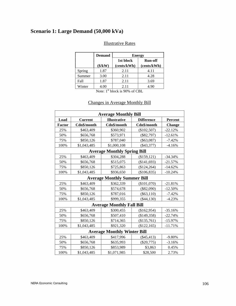
Scenario 1: Large Demand (50,000 kVa)
Illustrative Rates
Demand Energy 1st block Run-off ($/kW) (cents/kWh) (cents/kWh) Spring 1.87 2.11 4.11 Summer 3.00 2.11 4.28 Fall 1.87 2.11 3.69 Winter 4.00 2.11 4.90
Note: 1st block is 90% of CBL
Changes in Average Monthly Bill
Average Monthly Bill Load Current Illustrative Difference Percent
Factor Cdn$/month Cdn$/month Cdn$/month Change 25% $463,409 $360,902 ($102,507) -22.12% 50% $656,768 $573,971 ($82,797) -12.61% 75% $850,126 $787,040 ($63,087) -7.42%
100% $1,043,485 $1,000,108 ($43,377) -4.16% Average Monthly Spring Bill
25% $463,409 $304,288 ($159,121) -34.34% 50% $656,768 $515,075 ($141,693) -21.57% 75% $850,126 $725,863 ($124,264) -14.62%
100% $1,043,485 $936,650 ($106,835) -10.24% Average Monthly Summer Bill
25% $463,409 $362,339 ($101,070) -21.81% 50% $656,768 $574,678 ($82,090) -12.50% 75% $850,126 $787,016 ($63,110) -7.42%
100% $1,043,485 $999,355 ($44,130) -4.23% Average Monthly Fall Bill
25% $463,409 $300,455 ($162,954) -35.16% 50% $656,768 $507,410 ($149,358) -22.74% 75% $850,126 $714,365 ($135,761) -15.97%
100% $1,043,485 $921,320 ($122,165) -11.71% Average Monthly Winter Bill
25% $463,409 $417,996 ($45,413) -9.80% 50% $656,768 $635,993 ($20,775) -3.16% 75% $850,126 $853,989 $3,863 0.45%
100% $1,043,485 $1,071,985 $28,500 2.73%
NERA Economic Consulting 106

Scenario 2: Large Demand (50,000 kVa)
Illustrative Rates
Demand Energy Charges Charges Peak Shoulder Off-Peak First block ($/kVA) (cents/kWh) (cents/kWh) (cents/kWh) (cents/kWh) Spring 2.00 5.42 4.45 2.38 2.24 Summer 3.00 6.5 4.7 1.87 2.09 Fall 2.00 4.96 3.88 2.19 2.21 Winter 4.00 7.32 4.53 3.69 2.03
Note: 1st block is 90% of CBL
Changes in Average Monthly Bill
Average Monthly Bill Load Current Illustrative Difference Percent
Factor Cdn$/month Cdn$/month Cdn$/month Change 25% $463,409 $362,667 ($100,742) -21.74% 50% $656,768 $575,333 ($81,434) -12.40% 75% $850,126 $788,000 ($62,126) -7.31%
100% $1,043,485 $1,000,666 ($42,819) -4.10% Average Monthly Spring Bill
25% $463,409 $320,209 ($143,200) -30.90% 50% $656,768 $540,418 ($116,350) -17.72% 75% $850,126 $760,626 ($89,500) -10.53%
100% $1,043,485 $980,835 ($62,650) -6.00% Average Monthly Summer Bill
25% $463,409 $359,477 ($103,932) -22.43% 50% $656,768 $568,954 ($87,813) -13.37% 75% $850,126 $778,431 ($71,695) -8.43%
100% $1,043,485 $987,909 ($55,576) -5.33% Average Monthly Fall Bill
25% $463,409 $313,937 ($149,472) -32.25% 50% $656,768 $527,874 ($128,893) -19.63% 75% $850,126 $741,811 ($108,315) -12.74%
100% $1,043,485 $955,748 ($87,737) -8.41% Average Monthly Winter Bill
25% $463,409 $411,450 ($51,959) -11.21% 50% $656,768 $622,899 ($33,868) -5.16% 75% $850,126 $834,349 ($15,777) -1.86%
100% $1,043,485 $1,045,799 $2,314 0.22%
NERA Economic Consulting 107

Scenario 3: Large Demand (50,000 kVa)
Illustrative Rates
Energy Charges Peak Shoulder Off-Peak (cents/kWh) (cents/kWh) (cents/kWh) Spring 4.06 3.09 0.99 Summer 5.14 3.34 0.48 Fall 3.60 2.52 0.80 Winter 5.96 3.17 2.33
Changes in Average Monthly Bill
Average Monthly Bill
Load Current Illustrative Difference Percent Factor Cdn$/month Cdn$/month Cdn$/month Change 25% $463,409 $265,004 ($198,404) -42.81% 50% $656,768 $530,009 ($126,759) -19.30% 75% $850,126 $795,013 ($55,113) -6.48%
100% $1,043,485 $1,060,018 $16,533 1.58% Average Monthly Spring Bill
25% $463,409 $237,463 ($225,946) -48.76% 50% $656,768 $474,925 ($181,842) -27.69% 75% $850,126 $712,388 ($137,738) -16.20%
100% $1,043,485 $949,850 ($93,635) -8.97% Average Monthly Summer Bill
25% $463,409 $253,328 ($210,081) -45.33% 50% $656,768 $506,657 ($150,111) -22.86% 75% $850,126 $759,985 ($90,142) -10.60%
100% $1,043,485 $1,013,313 ($30,172) -2.89% Average Monthly Fall Bill
25% $463,409 $199,389 ($264,020) -56.97% 50% $656,768 $398,777 ($257,990) -39.28% 75% $850,126 $598,166 ($251,961) -29.64%
100% $1,043,485 $797,554 ($245,931) -23.57% Average Monthly Winter Bill
25% $463,409 $323,260 ($140,149) -30.24% 50% $656,768 $646,519 ($10,248) -1.56% 75% $850,126 $969,779 $119,652 14.07%
100% $1,043,485 $1,293,038 $249,553 23.92%
NERA Economic Consulting 108

Scenario 4: Large Demand (50,000 kVa)
Illustrative Rates
Demand Energy Charges
Charges Peak Shoulder Off-Peak ($/kVA) (cents/kWh) (cents/kWh) (cents/kWh) Spring 2.00 3.57 2.60 0.64 Summer 3.00 4.65 2.85 0.13 Fall 2.00 3.11 2.03 0.45 Winter 4.00 5.47 2.68 1.84
Changes in Average Monthly Bill
Average Monthly Bill
Load Current Illustrative Difference Percent Factor Cdn$/month Cdn$/month Cdn$/month Change
25% $463,409 $373,175 ($90,234) -19.47% 50% $656,768 $596,350 ($60,418) -9.20% 75% $850,126 $819,525 ($30,602) -3.60%
100% $1,043,485 $1,042,699 ($786) -0.08% Average Monthly Spring Bill
25% $463,409 $297,068 ($166,341) -35.90% 50% $656,768 $494,136 ($162,631) -24.76% 75% $850,126 $691,204 ($158,922) -18.69%
100% $1,043,485 $888,272 ($155,213) -14.87% Average Monthly Summer Bill
25% $463,409 $362,959 ($100,450) -21.68% 50% $656,768 $575,919 ($80,849) -12.31% 75% $850,126 $788,878 ($61,249) -7.20%
100% $1,043,485 $1,001,837 ($41,648) -3.99% Average Monthly Fall Bill
25% $463,409 $258,968 ($204,440) -44.12% 50% $656,768 $417,937 ($238,831) -36.36% 75% $850,126 $576,905 ($273,221) -32.14%
100% $1,043,485 $735,874 ($307,611) -29.48% Average Monthly Winter Bill
25% $463,409 $478,547 $15,138 3.27% 50% $656,768 $757,094 $100,327 15.28% 75% $850,126 $1,035,641 $185,515 21.82%
100% $1,043,485 $1,314,188 $270,703 25.94%
NERA Economic Consulting 109

National Economic Research Associates, Inc. 777 South Figueroa Street, Suite 1950 Los Angeles, CA 90017 213 346 3000
NERA Economic Consulting 110