Embed Size (px)
Citation preview
Received January 5, 2021, accepted January 21, 2021, date of publication February 1, 2021, date of current version February 10, 2021.
Digital Object Identifier 10.1109/ACCESS.2021.3056003
Review on Fuzzy and Neural Prediction IntervalModelling for Nonlinear Dynamical SystemsOSCAR CARTAGENA 1, (Graduate Student Member, IEEE),SEBASTIÁN PARRA1, (Member, IEEE), DIEGO MUÑOZ-CARPINTERO2, (Member, IEEE),LUIS G. MARÍN3, (Member, IEEE), AND DORIS SÁEZ 1,4, (Senior Member, IEEE)1Department of Electrical Engineering, Faculty of Mathematical and Physical Sciences, University of Chile, Santiago 8370451, Chile2Institute of Engineering Sciences, Universidad de O’Higgins, Rancagua 2841935, Chile3Department of Electrical and Electronics Engineering, Universidad de Los Andes, Bogotá 111711, Colombia4Instituto Sistemas Complejos de Ingeniería, Santiago 8370451, Chile
Corresponding author: Doris Sáez ([email protected])
This study was supported by the Fondo Nacional de Desarrollo Cientìfico y Tecnològico (FONDECYT) under grant 1170683, the SolarEnergy Research Center SERC-Chile under grant ANID/FONDAP/15110019, Instituto Sistemas Complejos de Ingeniería (ISCI) undergrant ANID PIA/BASAL AFB180003 and ANID/PAI Convocatoria Nacional Subvención a Instalación en la Academia Convocatoria 2019PAI77190021. The work of Oscar Cartagena was supported by the ANID-PFCHA/Doctorado Nacional/2020-21200709.
ABSTRACT The existing uncertainties during the operation of processes could strongly affect the perfor-mance of forecasting systems, control strategies and fault detection systems when they are not consideredin the design. Because of that, the study of uncertainty quantification has gained more attention amongthe researchers during past decades. From this field of study, the prediction intervals arise as one of thetechniquesmost used in literature to represent the effect of uncertainty over the future process behavior. Thus,researchers have focused on developing prediction intervals based on the use of fuzzy systems and neuralnetworks, thanks to their usefulness for represent a wide range of processes as universal approximators.In this work, a review of the state-of-the-art of methodologies for prediction interval modelling based onfuzzy systems and neural networks is presented. The main characteristics of each method for predictioninterval construction are presented and some recommendations are given for selecting the most appropriatemethod for specific applications. To illustrate the advantages of these methodologies, a comparative analysisof selected methods of prediction intervals is presented, using a benchmark series and real data from solarpower generation of a microgrid.
INDEX TERMS Prediction intervals, fuzzy interval, neural network intervals, uncertainty.
I. INTRODUCTIONThe use of fuzzy logic systems (FLS) and neural net-works (NNs) has proliferated in the literature for themodelingof systems and time series. Since both types of models areknown as universal approximators that can identify relation-ships between inputs and target (outputs) variables, they aregenerally used when the system or the time series to be mod-eled follows nonlinear dynamics [1]. Although FLS and NNexhibit adequate performance to obtain the expected value ofthese kind of systems, uncertainty is not typically quantifiedby these modelling approaches. However, information on thedispersion of the output of the model provides more informa-tion about the phenomena. and more useful information from
The associate editor coordinating the review of this manuscript and
approving it for publication was Valentina E. Balas .
a decision-making point of view than the models with onlyexpected values [2], [3].
Prediction intervals have been proposed to address theproblematic of quantifying prediction uncertainty. A predic-tion interval establishes a range around the output of themodel, representing the uncertainty present in the system.The main motivation for the construction of prediction inter-vals is to quantify the uncertainty in the point predictionto provide information about the uncertainty and enable theconsideration of multiple scenarios for the best and worstconditions of the system [4].
Usually the width of the prediction interval increases withthe prediction horizon due to the coupling effect and prop-agation of the different sources of uncertainty in the model.In several applications, such as the implementation of fore-casting systems, control strategies, fault detection methods
VOLUME 9, 2021 This work is licensed under a Creative Commons Attribution 4.0 License. For more information, see https://creativecommons.org/licenses/by/4.0/ 23357
O. Cartagena et al.: Review on Fuzzy and Neural Prediction Interval Modelling for Nonlinear Dynamical Systems
or decision support systems, where decisions are taken basedon the predicted future behavior of the modeled system, it isdesired that the prediction intervals are as precise as possible.Therefore, the aim to prediction interval construction is tofind the narrowest intervals possible that contain a desiredpercentage of measured data over the future time horizon.
Considering the importance of FLS and NN for the mod-eling of nonlinear systems and time series, several methodshave been proposed in order to construct an appropriate pre-diction interval based on these models. The main contributionof this paper is to analyze and compare features and theperformance of the methods for construction of predictionintervals based on FLS and NN reported in the special-ized literature. In order to evaluate the prediction intervalsperformance, several methods are compared based on twodynamical nonlinear systems implemented: modified Chenseries and solar power generation data from Milan. Finally,the characteristics and applicability of each discussed meth-ods are presented.
The remainder of this paper is organized as follows:Section II presents the fundamentals of prediction intervals.Sequential and direct methods for both fuzzy and neuralprediction intervals construction are described in section IIIand IV respectively. The characteristics and a discussion ofthe methods are presented in section V. Section VI presentsthe results of a benchmark test and case study from solarpower generation of a microgrid. The last section providesthe main conclusions.
II. FUNDAMENTALS OF PREDICTION INTERVALSA. SOURCES OF UNCERTAINTY IN SYSTEM MODELINGIn order to fully understand the information provided byPrediction Intervals, it is important to study what are thepossible causes of uncertainty in dynamical systemmodeling,and on what phenomena they can originate.
In theory, predictive modeling assumes that all observa-tions are generated by a data generating function f (x) com-bined with and additive noise [4]–[6]
y = f (x)+ ε, (1)
where ε is a zero mean random variable called data noisethat is responsible for introducing uncertainty modeling intopredictivemodels in the form of aleatory uncertainty, whoseorigin can be traced to the exclusion of complicated variablesfrom the model which cannot be determined with sufficientprecision, or due to the presence of inherently stochasticprocesses in the observed system or data obtention procedure.
Based on this formulation, predictive models attempt toproduce an estimate f (x) of the data generating function inorder to calculate predictions of the expected value of thesystem. The model of f (x) is often referred to as crisp model.This procedure introduces an additional form of uncertainty,known as epistemic uncertainty, since the crisp model isonly an approximation of the true data generating function.Assuming both types of uncertainty are independent, the total
variance of observations can be expressed as
σ 2total = σ
2model + σ
2data (2)
where σ 2model is attributed to epistemic uncertainty and σ 2
datais attributed to aleatory uncertainty.
Since the factors contributing to epistemic uncertainty canvary greatly, some authors [7] have proposed subsequentclassifications for this term:
1) Model misspecification: Uncertainty determined byhow close the estimate f (x) can approximate the realdata generating function f (x) under optimal parameterand data conditions
2) Training data uncertainty:Uncertainty over how rep-resentative the training data is with respect to the wholeinput distribution, and how sensitive the model can beto unseen samples
3) Parameter uncertainty: Uncertainty on the values ofthe model parameters due to local minima stagnationor premature termination.
It is important to note that since total uncertainty can comefrommany diverse sources, the expression can be highly com-plex and difficult to quantify, which is why interval modelinghas been proposed as a solution to this problem.
B. TYPES OF INTERVALS AND PREDICTION INTERVALMETHODSRegarding to interval models it is important to differentiateconfidence intervals from prediction intervals.
Strictly speaking, f (x) is a prediction of f (x), the trueregression mean of y as shown in (1). A confidence inter-val (CI) is an estimate, obtained from observed data, of aninterval where the true mean of f (x) must lie with a givenconfidence. In this sense, the CI deals with the uncertainty off (x) to estimate f (x), i.e. the epistemic uncertainty. A predic-tion interval (PI), on the other hand, quantifies the uncertaintyof using f (x) to predict y; it defines an interval where theobservations of y must fall inside the interval with a givenprobability. Therefore, in addition to the epistemic uncer-tainty, the PI must also account for the aleatory uncertainty.
According to the concepts above, a CI is based on thecharacteristics of P(f (x)|f (x)), and a PI is based on the char-acteristics of P(y|f (x)). It is easy to see that PIs are wider thanCIs. In this work the focus is on PIs as we are interested inthe uncertainty of using f (x) for predicting y.
The reason for the focus on intervalmodels, PIs in this case,is that they are a useful and practical tool for expressing theuncertainty of the predictions with the minimum information.Only three outputs are needed: an upper bound (y), the lowerbound (y) and the coverage probability (PICP, as it will bedefined later). This is enough to inform the most probablerange and the probability of enclosure. In contrast, probabilitydensity functions (PDFs) contains exact information aboutthe uncertainty. However, in practice, only particular distribu-tions can be described with few parameters. For the generalcase, a large number of points is needed to approximate(up to a grid precision) the PDFs. Therefore, PIs are the
23358 VOLUME 9, 2021
O. Cartagena et al.: Review on Fuzzy and Neural Prediction Interval Modelling for Nonlinear Dynamical Systems
most understandable uncertainty quantification mechanismthat uses few parameters in the general case.
There is a wide variety of methods to construct PIs. Forthis, we want to find the lower and upper bounds y, y so thaty ∈ [y, y] with probability 1− p, i.e.
P(y ≤ y ≤ y) = 1− p. (3)
A basic method to find these bounds relies on the use ofthe PDF of y, which is assumed known. If the probabil-ity that y is outside this interval is chosen to be the sameabove and below the interval, the bounds can be found asy = F−1(p/2) and y = F−1(1 − p/2), where F−1( · ) isthe inverse of the distribution function of y. This can beperformed with known parametric PDFs or with PDFs withany non-parametric estimation. However, in practice a PDFcannot be estimated perfectly, and therefore therewill be errorpropagation when computing the interval. For this reason,if one is only interested in the PI and does not need all theinformation in the PDF, it is more convenient to use a methodthat estimates the PI without needing a known PDF.
C. NOTATION FOR DYNAMICAL SYSTEMSIn this review we focus on methods based on computationalintelligence that directly construct the PIs for dynamical sys-tems, in particular those based on fuzzy models and neuralnetworks. Here, in order to establish the notation to be usedfor the inputs variables of the different methods to be covered,it is assumed that the system to bemodeled follows a dynamicdescribed by a nonlinear autoregressive exogenous model(NARX), i.e. the output of the system is given by
y(k) = f (zk ), (4)
where zk is the input vector of size nz, composed by the pastny outputs y and the past nu exogenous variables u, such thatthe input vector is defined as
zk =[y(k − 1), y(k − 2), . . . , y(k − ny),
u(k − 1), u(k − 2), . . . , u(k − nu)]T . (5)
D. PREDICTION INTERVAL METRICSSeveral metrics have been used in the literature to design,validate and compare the effectiveness of prediction intervals.The most standard metrics, which will be used in this work,are presented next.
The prediction error of the crisp model is one of the mostimportant factors that affects the behavior of the uncertaintyband. In order to represent the accuracy of the predictivemodel, the root mean square error (RMSE)
RMSE =
√√√√ 1N
N∑k=1
(y(k)− y(zk ))2, (6)
is selected in this work as the metric for representing theaccuracy of the predictive model. In (6), N is the number ofdata selected for the computation of this metric, y(k) is thereal measurement of the system of signal output, and y(zk )) is
the predicted value given by the identified model when theinput vector zk is received.
The interval width and coverage level are remaining mostimportant metrics. In [4], [8], the Prediction Interval Normal-ized Averaged Width (PINAW) and the Prediction IntervalCoverage Probability (PICP) are defined respectively for rep-resenting those factors, based on the following expressions:
PINAW =1NR
N∑k=1
(y(zk )− y(zk )
), (7)
where
R = max {y(k)} −min {y(k)} (8)
is the range of values of the training data, and
PICP =1N
N∑k=1
ck , (9)
where
ck =
{1, if y(zk ) ≤ yk ≤ y(zk )0, otherwise
(10)
indicates if the interval given by the bounds [y(zk ), y(zk )],contains the real measure of y(k).
E. CLASSIFICATION OF METHODS FOR THIS SURVEYGiven that there is a wide variety of methods for PI construc-tion as discussed above, a proper classification of themethodsto be included in this survey is in place. This classificationwill be based on two main criteria: (i) type of model used todescribe the prediction interval, and (ii) the type of trainingprocedure for PI construction.
Given the scope of this survey, the type of base modelused for the PI methods defines the following division con-sidered for this paper: (a) methods based on fuzzy models,and (b) methods based on neural networks.
On the other hand, considering the type of training, firstcategorization corresponds to Sequential methods, whichreceives a previously identified base crisp model that esti-mates f (x) and then uses it to constructed the PI in a sub-sequent step. The second category, which will be referred toas Direct methods, perform the construction of the intervalmodels in parallel with the crisp model identification. There-fore, a previously identified model is not required for thiscase. In this type ofmethods, the training process of themodelincorporates the calculations to estimate the uncertainty bandof the predictions, so that the models obtained are capable ofdirectly outputting a prediction interval without the need ofadditional steps.
This classification scheme is shown in Table 1. Accordingto it, the methods studied in the context of this work arepresented in the following order: the sequential and directmethods developed based on fuzzy models are presented firstin section III. Then, the sequential and direct methods basedon neural networks are described in section IV.
VOLUME 9, 2021 23359
O. Cartagena et al.: Review on Fuzzy and Neural Prediction Interval Modelling for Nonlinear Dynamical Systems
TABLE 1. Classification of PI construction methods considered for thissurvey.
III. FUZZY PREDICTION INTERVALSA. BACKGROUNDRule-based FLS are considered for solving a broad rangeof problems, from forecasting, to classification, control, etc.Because of this, the use of prediction intervals based on thesemodels arises as an important way to include informationabout uncertainty in the implementation of forecasting sys-tems and control strategies.
Among rule-based fuzzy models, the formulation pre-sented by [9] arise as one of the most used structure for rulebase fuzzy modeling. The fuzzy model of Takagi and Sugenoof this formulation is represented by the weighted sum ofseveral linear models, as shown as follows
Rule r: If zk is Ar , then: yr (zk ) = [1 zTk ]θr , (11)
y(zk ) =m∑r=1
βr (zk )yr (zk ) (12)
where zk is the input vector of the fuzzy model at instant k(see equation (5)), Ar is a fuzzy set (antecedents) and yr isthe output of the local model (consequences) for rule r .The model consists of m rules so that r = 1, . . . ,m.For each rule r in (11), θr is the parameter vector, whichcan be obtained using a suitable regression algorithm, andβr (z) corresponds to the degree of activation of the rule. Thevalues of βr (z) are calculated from the membership func-tions (MF) of the fuzzy sets which are part of the antecedentsof the rule r.
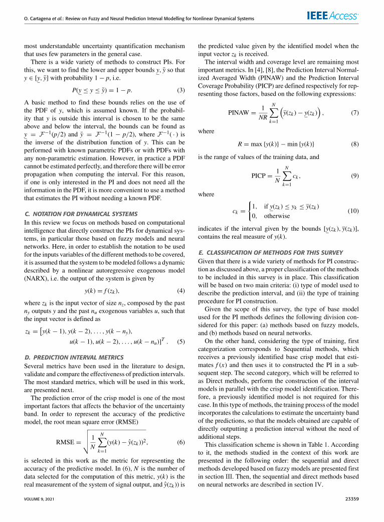
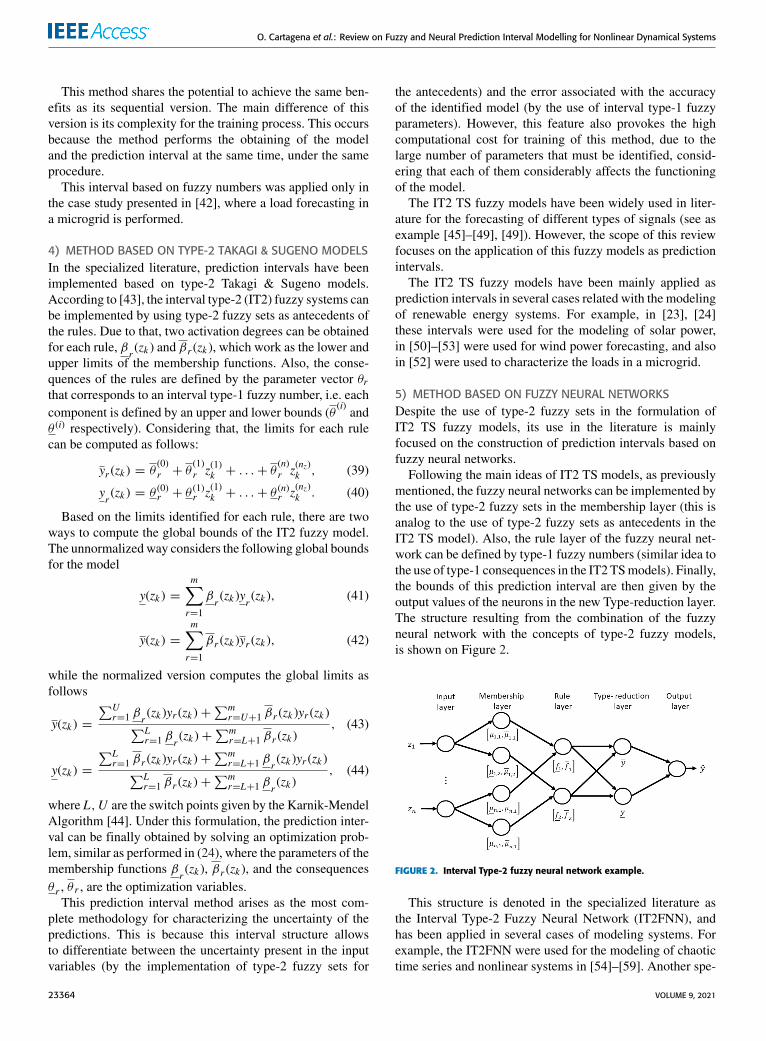
In order to consider the effect of uncertainties in the modelidentification, the type-2 fuzzy models presented in [10] ariseas an appropriate extension of the fuzzy rule-based models.In this case, type-2 fuzzy sets, which are originally introducedin [11], are used for the antecedents of the rules. Thus,as shown in Figure 1, a type-2 fuzzy set A has a membershipfunction defined by two different values, corresponding to itsupper and lower limits (µA(x) and µA(x) respectively).The value of the membership function lies inside this gray
area bounded by µA(x), µA(x), which is denominated in
literature as the domain of uncertainty of A (DOU(A)) or thefootprint of uncertainty ofA (FOU(A)). Due to the use of thesetype-2 fuzzy sets the local outputs of the rules are now definedby an upper and lower value. Note that, this kind ofmodels aresuited for the later implementation of the prediction intervals.
Fuzzy models have also been implemented in the literatureas fuzzy neural networks (FNN) [12], [13]. These imple-mentations result from the adaptation of TS fuzzy modelsto the artificial neural networks structure. The stages definedfor TS models are handled by different layers of the neural
FIGURE 1. Type-2 membership function.
network in FNNs, such that each of the antecedents and theconsequences of the rules have their own neurons associated.
In the specialized literature, several methods based onTakagi-Sugeno fuzzy models have been proposed in orderto obtain a Prediction Interval. As mentioned in section II-E,those methods are classified by the type of training procedurefor its construction.
The fuzzy interval models of both categories, correspond-ing to sequential and direct methods, are reviewed below.
B. SEQUENTIAL METHODS1) COVARIANCE METHODIn [14], the upper and lower bounds that define the intervalare constructed based on the error covariance of each ruleof the Takagi-Sugeno fuzzy model. This strategy of fuzzyPI design is referred in the literature as the covariance methodand it is based on the work done by Škrjanc in [15]. For aninput vector zk , the bounds of the local model r , for eachmeasurement k are defined as
yr (zk ) = yr (zk )+ αIr (zk ), (13)
yr(zk ) = yr (zk )− αIr (zk ). (14)
where α is a tuning parameter and Ir is an estimate of thevariance of yr . The estimate Ir is given by
Ir (zk ) = σr(I + ψT
r (zk )[9r9
Tr
]−1ψr (zk )
)1/2
, (15)
where I is an identity matrix of appropriate size;σ 2r I is the variance of the noise signal; and 9r =
[ψr (z1), . . . , ψr (zM )]T is the regression matrix that containsthe regression vectors (past values of ψT
r (z) = [1 zTk ] in theTS fuzzy model) for theM samples of a training dataset.This method of fuzzy prediction interval design resembles
the defuzzification stage performed in the aforementionedmethods, which follow the idea presented in (12). Here,a global value for the estimated variance of y is obtained as
I(zk ) =m∑r=1
βr (zk )Ir (zk ). (16)
23360 VOLUME 9, 2021
O. Cartagena et al.: Review on Fuzzy and Neural Prediction Interval Modelling for Nonlinear Dynamical Systems
Thus, the bounds of the global output of the fuzzy intervalmodel is given by
y(zk ) = y(zk )+ αI(zk ), (17)
y(zk ) = y(zk )− αI(zk ). (18)
This method for the prediction interval construction has themain advantage of a low computational cost for obtaining theinterval. This is because the uncertainty is estimated directlyby the given covariance formula. Thus, the main complexityof this method lies in the search of the proper values forthe tuning parameters α. On the other hand, this intervalstructure presents a weakness in differentiating the effect ofinternal and external sources of uncertainty. This is a cleardisadvantage of this method, because the performance of theprediction interval will be negatively affected when trying tomodel a systemwith exogenous input variables that have theirown uncertainty.
This method has been applied in [14] for the forecastingof renewable generation and demand data from an installedmicrogrid and in [16] for the robust control of a solar collectorfield. Also, in [17] is applied in a fault detection system foran aircraft, and in [18] is used for an implementation of anindoor localization algorithm.
Additionally, some versions of this method have beendeveloped in order to reduce the interval width. For exam-ple, in [19] different tuning parameters were proposed forthe upper and lower bounds (α and α respectively), achiev-ing a non-symmetrical interval around the prediction value.This version of the method has been applied in [19] forthe identification of intervals for traffic measurements, andin [20], [21] for the forecasting of renewable generationand demand data from an installed microgrid. Later, a thirdversion of this method was proposed in [22], where the tuningparameters can also vary depending of the instant k when thepredictions are made (αk ). This is done in order to adjust theinterval width to the specific cases of signals with uncertaintybehaviors strongly dependent on the time of day, such as thecases of solar generation and occupancy level of offices. Thisversion was only used in [22] for a robust predictive controldesign applied on a climatization system.
2) METHOD BASED ON INTERVAL FUZZY NUMBER FOR THEOUTPUT UNCERTAINTYIn [23], an interval is proposed from a Takagi-Sugeno fuzzymodel. In that case, after that the model is identified, a singleinterval fuzzy number is added in order to approximate themodel uncertainties present in the output of the system. Thatinterval was later denoted in [24] as A1-C1 Takagi-Sugeno(TS), because is defined by type-1 antecedents and conse-quences. This interval is defined in [23] as
yr = fr (x)+ a, a ∈ A0 ={a0,∈ [a0, a0], µA(t)
}, (19)
where yr is the output and fr is the local model identified,both for each rule r . Also in (19), A0 is a type-1 fuzzy setdefined by the bounds [a0, a0] (which are obtained from
the knowledge of the uncertainties given by the error of themodel) and the membership function µA(t).This method presents its low computational cost to obtain
the interval as its main advantage. This is because the con-struction of the interval is reduced to identifying a singlefuzzy number. However, this feature also causes the maindisadvantage of this method, which is that its use is very situ-ational. A reliable prediction interval can be generated whenexternal disturbances act as the only source of uncertaintyaffecting the system.
The intervals obtained with this method have been appliedfor the forecasting of solar power generation in [23], [24].
3) METHOD BASED ON FUZZY NUMBERS (SEQUENTIALVERSION)In the work [2], another version of fuzzy interval is pro-posed, based on the idea of intervals fuzzy numbers presentedin [25]. In this method, the parameters of the consequencesare defined by fuzzy numbers, thus, the output of the fuzzyinterval for each rule r is given by the bounds
y(zk ) =nz∑i=1
g(i)r z(i)k + g
(0)r +
nz∑i=1
s(i)r |z(i)k | + s
(0)r , (20)
y(zk ) =nz∑i=1
g(i)r z(i)k + g
(0)r −
nz∑i=1
s(i)r |z(i)k | − s
(0)r , (21)
where zk is the input vector of the fuzzy model at instant k .In (20)-(21), g(i)r are the mean values and s(i)r ,s(i)r are thespread values of the parameter θ (i)r which is associated to thei-th component of zk . Then, the global bounds of the fuzzyinterval are obtained as
y(zk ) =m∑r=1
βr (zk )yr (zk ), (22)
y(zk ) =m∑r=1
βr (zk )yr (zk ), (23)
In the direct version of this method, the fuzzy model hasalready been identified, so the mean values of the parametersg(i)r are assumed known. Thus, the interval identification con-sist in obtaining the spread values (s(i)r , s(i)r ) from solving thefollowing optimization problem:
minsr ,sr
PINAW
s.t. PICP = (1− α)%, (24)
The equality constraint PICP = (1 − α)% is a hardconstraint, and due to the nonlinear characteristic of the opti-mization problem (24), it could be difficult to solve with thetypical algorithms. With the purpose of relaxing this equalityconstraint, a version of the optimization problem is proposedin [2], which includes that constraint as a barrier function.Such that, the interval identification can also be defined bythe following optimization problem:
minsi,si
J = η1PINAW+ exp{−η2 [PICP− (1− α)]}. (25)
VOLUME 9, 2021 23361
O. Cartagena et al.: Review on Fuzzy and Neural Prediction Interval Modelling for Nonlinear Dynamical Systems
This method for the prediction interval constructionpresents an increment of the computational cost when com-pared with the previous methods, due to the higher number ofparameters that need to be identified. This inclusion of moreparameters, like the separated spread values, allows to obtainmore precise prediction intervals when dealing with systemswith complex uncertainty behavior (such as non-Gaussian orheteroscedastic noise).
This interval method based on fuzzy numbers was appliedin the case study presented in [2], which consists in the fore-casting of the load in a microgrid and the energy consumptionin some residential dwellings.
4) METHOD BASED ON α-LEVEL CUTS OF THE OUTPUTIn the work of [26] a Mamdani fuzzy logic system based onα-level cuts of the output is presented to generate the predic-tion intervals. An α-cut of a fuzzy set A is a crisp set Aα thatcontains all the elements in U that have membership valuesin A greater than or equal to α, that is [27],
Aα = {x ∈ U | µA(x) ≥ (α)}. (26)
The general idea to obtain the prediction interval based onalpha-cut (α) approach is to decompose output fuzzy sets intoa collection of crisp sets related together via the α levels [28].Therefore, Alpha cuts on Mamdani Fuzzy logic system basedoutput fuzzy sets (commonly defuzzified to a crisp number)are used to provide this prediction interval using the following4-step process [26]:
• FLS Desing: A Mamdani FLS is designed to obtainthe expected value of the system prediction. Standardapproaches to FLS prediction are applied.
• Generating Output Fuzzy Sets: After constructing thestandard Mamdani FLS, the inferencing over the inputFuzzy Sets and the rules are processed with conventionaloperators. By implementing the selected operators in theinference step, the output Fuzzy Sets of the MamdaniFLSs are generated.
• Defining alpha-cut level: There are several options toselect an appropriate level of α for a given application.In general, the higher the selected value of α, the morenarrow the output prediction interval. However, someα levels (those which are greater than the height of theoutput Fuzzy Set) may not result in any prediction inter-val output (alpha-cut is an empty set). In addition, someα levels may lead the traditional centroid defuzzifica-tion results falling outside of the generated predictionintervals.
• Generate alpha cut and centroid based outputs: Basedon the selected α-level, the support is used as the pre-diction interval. Thereafter, a defuzzification techniqueis implemented on the gathered output set and a crispvalue is calculated.
The proposed method was explored using both synthetic(Chaotic Mackey-Glass) and smart-grid specific real-world(wind power) time series datasets for one-step ahead.
With the sequential methods based on the fuzzy modelsalready covered in this review, now the intervals of the sec-ond category aforementioned (the direct methods) will beexplained below.
C. DIRECT METHODS1) MIN-MAX METHODThe main idea of this kind of methods was introduced in [29],where a min-max method is proposed for identifying thebounds of the fuzzy interval. Then, the interval is obtained bythe identification of two different fuzzy functions, called theupper and lower functions (f (z) and f (z) respectively), whichare found by solving the following min-max optimizationproblems:
minf
maxzi∈Z|yi − f (zi)| subject to yi − f (zi) ≤ 0, ∀i, (27)
minf
maxzi∈Z|yi − f (zi)| subject to yi − f (zi) ≥ 0, ∀i, (28)
where zi is the i-th sample of the training dataset Z , and yi isthe i-th measured output. Thus, the bounds of the predictioninterval asociated to the input zk are given by
y = f (zk ) =m∑r=1
βr (zk )θ rzk , (29)
y = f (zk ) =m∑r=1
βr (zk )θ rzk , (30)
where θ r and θ r are the parameter vectors of the fuzzyfunctions obtained in (27) and (28) respectively.
The advantage of this method is its great flexibility formodeling the behavior of prediction error variance. This fea-ture is present thanks to the identification of two differentmodels for representing the bounds of the prediction uncer-tainty. However, the use of two computationally min-maxproblems, increases the requirements that the selected opti-mization algorithm must meet in order to obtain accurateresults. Furthermore, this method does not offer a directmechanism to properly sets the expected values for the widthand coverage level of the intervals. Thus, if a specific cover-age level is wanted for the prediction interval, some variationsof the (27)-(28) should be developed first.
The min-max method was applied to the fault detec-tion problem over various type of systems. In [30] thismethod was used to detect the fault in a Motor-GeneratorPlant, in [31]–[33] the formulation of a fault-detection sys-tem for a nonlinear system with uncertain parameters, andin [34] this method was used for the construction of a beliefrule-based model for the identification problem of uncertainnonlinear systems. Also, in [35]–[37] the fuzzy intervalsbased in this method were used in the implementation ofa robust control strategy and in [36]–[38] were applied inthe estimation of time-series related with renewable energysystems.
23362 VOLUME 9, 2021
O. Cartagena et al.: Review on Fuzzy and Neural Prediction Interval Modelling for Nonlinear Dynamical Systems
2) METHOD BASED ON INTERVAL-VALUED DATAIn [39] another version of fuzzy interval models was pro-posed, based in the use of interval arithmetic for the mod-eling of an interval valued output. Under this formulation,the output signal Y to be modeled must be an interval-valueddata defined by a center and a radius, i.e. Y = (Ya,Yc).In this approach, and following the formulation of TS fuzzymodels (11)-(12), different local models are identified for theinterval-valued output. Thus, for each rule r , the respectivelocal model has the form
Yr (zk ) = θTr zk , (31)
where each component of the vector θTr = [θ (0)r , . . . , θ(n)r ]
are interval-valued parameters defined by a correspondingcenter a(i)r and a radius c(i)r , such that
θ (i)r = (a(i)r , c(i)r ). (32)
Note that, this definition of the model is only valid whenthe input vector zk is made up of crisp values. However,the dynamical interval Takagi-Sugeno fuzzy model proposedin [39] considers a mixed typed identification problem (there,zk can be made up of interval-valued and crisp data). Consid-ering this, the local rules presented in (31) can be rewritten asfollows:
If Y (k − 1) is Ar,1, . . . ,Y (k − nY ) is Ar,nY , u(k − 1) isBr,1, . . . , u(k − nu) is Br,nu , then:
Yr (zk ) = Pr,0 +nY∑j=1
Y (k − j) ◦ Pr,j
+
nu∑l=1
u(k − l)Pr,nY+l, (33)
where Ar,i and Br,i are the fuzzy sets associated toY (k−j) and u(k−j) respectively. Note that, since Y (k−j) is aninterval-valued data, Ar,i must be composed by two differentfuzzy sets, such that, one is associated to the center value ofY (k − j) (denoted as Aar,i), meanwhile the other correspondto its radius (denoted as Acr,i). Also in (33), the values Pr,ifor i = 1, . . . , nY are the crisp components of the parametervector θr which multiply the interval-valued data Y (k − i).On the other hand, the values Pr,nY+l for l = 1, . . . , nu arethe interval-valued parameters that multiply the crisp inputvariable u(k − l).In order to obtain the prediction interval, the operator◦ included in (33) is proposed from the interval arith-metic developed in [39]. That operator is defined for aninterval-valued data (a, c) and a vector xT = [x11, x12,x21, x22, . . . , xn1, xn2] as follows
(a, c) ◦ x =
(ax11, c|x12|)...
(axn1, c|xn2|)
. (34)
Following the formulation of the global output of theTakagi-Sugeno fuzzy model presented in (12), the output of
the proposed interval is represented by
Y (zk ) =m∑r=1
βr Yr (zk ) (35)
This interval method has the low computational cost forthe training process as its main advantage. This low cost ispresented because the method uses data which are alreadybeen characterized by an interval, so the identified modelgives directly the bounds for the predictions thanks to theinterval arithmetic. Due to that, this interval constructionmethod is similar in complexity to the identification processof a classic fuzzy TS model. However, this interval structurehas the difference of a large quantity of parameters that needto be identified. On the other hand, because this methodrequires the use of interval-valued data, its applicability isrestricted to the availability of these types of signals.
This interval method presented in (35) is applied in [39]for the identification of a nonlinear system. A similar strat-egy was followed in the works of [40], [41], where a fuzzymodel is identified for an interval-valued data characterizedby confidence intervals obtained from an electro-mechanicalthrottle valve using the Chebyshev’s inequality.
3) METHOD BASED ON FUZZY NUMBERS (DIRECTVERSION)In the work [42], an alternative version of the method basedon intervals fuzzy numbers is proposed. The parameters of theconsequences are defined by fuzzy numbers, thus, the outputof the fuzzy interval for each rule r is given by the bounds
yr (zk ) =nz∑i=1
g(i)r z(i)k + g
(0)r +
nz∑i=1
s(i)r |z(i)k | + s
(0)r , (36)
yr(zk ) =
nz∑i=1
g(i)r z(i)k + g
(0)r −
nz∑i=1
s(i)r |z(i)k | − s
(0)r , (37)
where g(i)r are the mean values and s(i)r are the spread valuesof the parameter θ (i)r . Then, the global bounds of the fuzzyinterval are given by the same bounds (22)-(23) used in thesequential version of this method.
In this version of the method, the construction of theinterval fuzzy model, considers the identification of bothvalues g(i)r and s(i)r performed at the same time (withoutthe classical identification of the TS model required in thesequential version). In order to achieve that, an optimizationproblem is proposed in [42], which minimize the followingmulti-objective cost function,
V = η1 MSE+ η2 PINAW+ η3 (ν(PICP− PICPD))2,
(38)
where PICPD is the desired coverage probability for theprediction interval, ν regulates the size of the allowed PICPerror and η1, η2, and η3 are weighing factors. Because theoptimization is nonlinear, the problem is solved in [42] usingthe Particle Swarm Optimization (PSO) and the ImprovedTeaching Learning Based Optimization.
VOLUME 9, 2021 23363
O. Cartagena et al.: Review on Fuzzy and Neural Prediction Interval Modelling for Nonlinear Dynamical Systems
This method shares the potential to achieve the same ben-efits as its sequential version. The main difference of thisversion is its complexity for the training process. This occursbecause the method performs the obtaining of the modeland the prediction interval at the same time, under the sameprocedure.
This interval based on fuzzy numbers was applied only inthe case study presented in [42], where a load forecasting ina microgrid is performed.
4) METHOD BASED ON TYPE-2 TAKAGI & SUGENO MODELSIn the specialized literature, prediction intervals have beenimplemented based on type-2 Takagi & Sugeno models.According to [43], the interval type-2 (IT2) fuzzy systems canbe implemented by using type-2 fuzzy sets as antecedents ofthe rules. Due to that, two activation degrees can be obtainedfor each rule, β
r(zk ) and βr (zk ), which work as the lower and
upper limits of the membership functions. Also, the conse-quences of the rules are defined by the parameter vector θrthat corresponds to an interval type-1 fuzzy number, i.e. eachcomponent is defined by an upper and lower bounds (θ
(i)and
θ (i) respectively). Considering that, the limits for each rulecan be computed as follows:
yr (zk ) = θ(0)r + θ
(1)r z(1)k + . . .+ θ
(n)r z(nz)k , (39)
yr(zk ) = θ (0)r + θ
(1)r z(1)k + . . .+ θ
(n)r z(nz)k . (40)
Based on the limits identified for each rule, there are twoways to compute the global bounds of the IT2 fuzzy model.The unnormalized way considers the following global boundsfor the model
y(zk ) =m∑r=1
βr(zk )yr (zk ), (41)
y(zk ) =m∑r=1
βr (zk )yr (zk ), (42)
while the normalized version computes the global limits asfollows
y(zk ) =
∑Ur=1 βr
(zk )yr (zk )+∑m
r=U+1 βr (zk )yr (zk )∑Lr=1 βr
(zk )+∑m
r=L+1 βr (zk ), (43)
y(zk ) =
∑Lr=1 βr (zk )yr (zk )+
∑mr=L+1 βr
(zk )yr (zk )∑Lr=1 βr (zk )+
∑mr=L+1 βr
(zk ), (44)
where L,U are the switch points given by the Karnik-MendelAlgorithm [44]. Under this formulation, the prediction inter-val can be finally obtained by solving an optimization prob-lem, similar as performed in (24), where the parameters of themembership functions β
r(zk ), βr (zk ), and the consequences
θ r , θ r , are the optimization variables.This prediction interval method arises as the most com-
plete methodology for characterizing the uncertainty of thepredictions. This is because this interval structure allowsto differentiate between the uncertainty present in the inputvariables (by the implementation of type-2 fuzzy sets for
the antecedents) and the error associated with the accuracyof the identified model (by the use of interval type-1 fuzzyparameters). However, this feature also provokes the highcomputational cost for training of this method, due to thelarge number of parameters that must be identified, consid-ering that each of them considerably affects the functioningof the model.
The IT2 TS fuzzy models have been widely used in liter-ature for the forecasting of different types of signals (see asexample [45]–[49], [49]). However, the scope of this reviewfocuses on the application of this fuzzy models as predictionintervals.
The IT2 TS fuzzy models have been mainly applied asprediction intervals in several cases related with the modelingof renewable energy systems. For example, in [23], [24]these intervals were used for the modeling of solar power,in [50]–[53] were used for wind power forecasting, and alsoin [52] were used to characterize the loads in a microgrid.
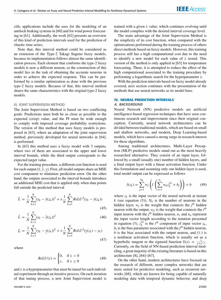
5) METHOD BASED ON FUZZY NEURAL NETWORKSDespite the use of type-2 fuzzy sets in the formulation ofIT2 TS fuzzy models, its use in the literature is mainlyfocused on the construction of prediction intervals based onfuzzy neural networks.
Following the main ideas of IT2 TS models, as previouslymentioned, the fuzzy neural networks can be implemented bythe use of type-2 fuzzy sets in the membership layer (this isanalog to the use of type-2 fuzzy sets as antecedents in theIT2 TS model). Also, the rule layer of the fuzzy neural net-work can be defined by type-1 fuzzy numbers (similar idea tothe use of type-1 consequences in the IT2 TSmodels). Finally,the bounds of this prediction interval are then given by theoutput values of the neurons in the new Type-reduction layer.The structure resulting from the combination of the fuzzyneural network with the concepts of type-2 fuzzy models,is shown on Figure 2.
FIGURE 2. Interval Type-2 fuzzy neural network example.
This structure is denoted in the specialized literature asthe Interval Type-2 Fuzzy Neural Network (IT2FNN), andhas been applied in several cases of modeling systems. Forexample, the IT2FNN were used for the modeling of chaotictime series and nonlinear systems in [54]–[59]. Another spe-
23364 VOLUME 9, 2021
O. Cartagena et al.: Review on Fuzzy and Neural Prediction Interval Modelling for Nonlinear Dynamical Systems
cific applications include the uses for the modeling of anantilock braking systems in [60] and for wind power forecast-ing in [61]. Additionally, the work [62] presents an overviewof this kind of prediction intervals used for the prediction ofchaotic time series.
Note that, this interval method could be considered asan extension of the Type-2 Takagi Sugeno fuzzy models,because its implementation follows almost the same identifi-cation process. Each element that conforms the type-2 fuzzymodels is now a different neuron, so the construction of thismodel lies in the task of obtaining the accurate neurons inorder to achieve the expected response. This can be per-formed by a similar optimization as done with the previoustype-2 fuzzy models. Because of that, this interval methodshares the same characteristics with the original type-2 fuzzymodels.
6) JOINT SUPERVISION METHODThe Joint Supervision Method is based on two conflictinggoals: Predictions must both be as close as possible to theexpected (crisp) value, and the PI must be wide enoughto comply with imposed coverage probability restrictions.The version of this method that uses fuzzy models is pro-posed in [63], where an adaptation of the joint supervisionmethod, previously developed for neural networks in [64],is performed.
In [63] this method uses a fuzzy model with 3 outputs,where two of them are associated to the upper and lowerinterval bounds, while the third output corresponds to theexpected target value.
For the training procedure, a different cost function is usedfor each output (y, y, y). First, all model outputs share anMSEcost component to minimize prediction error. On the otherhand, the outputs associated to the interval bounds introducean additional MSE cost that is applied only when data pointsfall outside the predicted interval
L =1N
N∑k=1
(yk − y(zk ))2 + λ1N
N∑k=1
ReLU2(yk − y(zk ))
(45)
L =1N
N∑k=1
(yk − y(zk ))2 (46)
L =1N
N∑k=1
(yk − y(zk ))2 + λ1N
N∑k=1
ReLU2(y(zk )− yk )
(47)
where
ReLU (x) =
{0, if x < 0x, if x ≥ 0
(48)
and λ is a hyperparameter that must be tuned for each individ-ual experiment through an iterative process. On each iterationof that tuning process, a new Joint Supervision model is
trained with a given λ value, which continues evolving untilthe model complies with the desired interval coverage level.
The main advantage of the Joint Supervision Method isthe simplicity of its cost function, when compared with theoptimizations performed during the training process of othersdirect methods based on fuzzy models. However, this trainingprocess still has a high computational cost due to the needto identify a new model for each value of λ tested. Thisversion of the method is only applied in [63] for temperatureforecasting. There, it is attempted to reduce the effect of thehigh computational associated to the training procedure byperforming a logarithmic search for the hyperparameter λ.With the prediction intervals based on fuzzy model already
covered, next section continues with the presentation of themethods that use neural networks as its model base.
IV. NEURAL PREDICTION INTERVALSA. BACKGROUNDNeural Network (NN) predictive models are artificialintelligence-based regression techniques that have seen con-tinuous research and improvement since their original con-ception. Currently, neural network architectures can bedivided between traditional models, which are based on smalland shallow networks, and modern, Deep Learning-basedmodels, which have caused a strong surge in research interestfor these algorithms.
Among traditional architectures, Multi-Layer Percep-tron (MLP) predictive models stand out as the most heavilyresearched alternative. They consist of an input layer, fol-lowed by a small (usually one) number of hidden layers, anda final output layer with a linear activation function. Underthis formulation and assuming only one hidden layer is used,total model output can be expressed as follows
y(zk ) =Nh∑j=1
wj
(f
( nz∑i=1
wjiz(i)k + bj
))+ b (49)
where zk is the input vector of the neural network at instantk (see equation (5)), Nh is the number of neurons in thehidden layer, wj is the weight that connects the jth hiddenneuron with the output, wji is the weight that connects the ith
input neuron with the jth hidden neuron, ny and nu representthe input vector length according to the notation presentedin equation (5), z(i)k is the ith component of input vector zk ,bj is the bias parameter associated with the jth hidden neuron,b is the bias associated with the output neuron, and f (·) isa nonlinear activation function, which is usually set as ahyperbolic tangent or the sigmoid function S(x) = 1
1+e−x .Currently, on the field of NN-based prediction interval mod-eling, a great majority of the existing literature is based on thisarchitecture [8], [64]–[67].
On the other hand, modern architectures have focused onthe research of different, more complex networks that aremore suited for predictive modeling, such as recurrent net-works [68], which are known for being capable of naturallymodeling data with temporal dynamic behavior, and deep
VOLUME 9, 2021 23365
O. Cartagena et al.: Review on Fuzzy and Neural Prediction Interval Modelling for Nonlinear Dynamical Systems
neural architectures, which have achieved better performancethan traditional networks by allowing the use of denser mod-els. Among these architectures, both shallow and deep LongShort-Term Memory (LSTM) networks [69] stand out as apopular alternative in predictive modeling that is also startingto see applications in prediction interval modeling [7], [70].
Aside from their structure, neural models can also varyon their training procedure. Since most of the modern workin literature is based on Deep Learning architectures, whichrequire fast and efficient training algorithms due to the sheeramount of parameters they have, the most commonly usedtechnique consists in stochastic gradient descent optimizationwith the help of the Backpropagation algorithm. This meansthe cost function’s gradient must be constantly calculated,which demands the use of simple and differentiable functions,such as Mean Square Error (MSE).
However, while the previous statement is true in the fieldof neural predictive modeling, NN-based prediction inter-val models may require a more flexible approach. This isbecause interval models rely on modified network archi-tectures adapted to produce a more informative output inthe shape of interval upper and lower bounds, resulting inan increase in model complexity. Because of this, somemethods must introduce more complex, nonlinear, or evennon-differentiable cost functions whose derivative cannotbe calculated in a closed form. Therefore, even though thestochastic gradient descent approach has proven to obtaingood results while minimizing computational costs, researchon neural interval models has also focused on evolutionarycomputing solutions, such as Genetic Algorithms [65] andParticle Swarm Optimization [66], [67]. Additionally, someniche cases also exist where the prediction interval con-struction method does not allow for any of these solutions,and instead requires a specific training methodology, suchas Bayesian approaches [71], which rely on Markov ChainMonte Carlo sampling algorithms.
The following subsections show a review of the neuralinterval models that can be found in the specialized litera-ture. As mentioned in section II-E, these methods have beencategorized into sequential and direct methods.
B. SEQUENTIAL METHODS1) DELTA METHODThis method [72] uses a strategy consisting of using classicalnonlinear regression theory to obtain an approximation of theprediction uncertainty. This can be done through the calcula-tion of the Taylor series expansion of the mean square errornetwork cost function. After this, assuming the noise varianceis homogeneous and normally distributed, total predictionvariance for each prediction can be represented as
σ 2tot (zk ) = σ
2ε (1+ g
T0 (J
T (zk )J (zk ))−1g0) (50)
where g0 represents the NN model parameters (weights andbiases), J (zk ) is the network’s Jacobian matrix evaluated oninput sample zk , and σε is the data noise variance, which can
be obtained from
σ 2ε =
1N
N∑k=1
(yk − y(zk ))2 (51)
where yk represents the training data point for sample k , andy(zk ) is the model prediction for input sample zk .
After calculating this value, the (1− α)% confidence pre-diction interval can be built, assuming it is symmetrical andGaussian, as
y(zk ) = y(zk )+ t1− α2n−p σtot (zk ) (52)
y(zk ) = y(zk )− t1− α2n−p σtot (zk ) (53)
where n is the number of input samples that were used totrain the model, p is the number of network parameters, andt1− α2n−p represents the α
2 quantile of a Student’s t-distributioncummulative distribution function with n − p degrees offreedom.
Due to relying on the assumption that the uncertaintymust be homogeneous and Gaussian, this method can fail toproduce quality PIs for applications where data noise variesthrough time. Additionally, since the Delta Method requiresthe calculation of the model Jacobian matrix, PI calcula-tion can be computationally expensive, which can make thismethod unfeasible for some online applications.
This method has seen applications in electricity load fore-casting [72], solder paste deposition process monitoring [73],indoor temperature and relative humidity prediction [74],groundwater quality monitoring [75] and travel timeprediction [76].
Finally, some versions of this method have been reported inliterature that improve its performance. For example, in [77],the authors propose the inclusion of a weight decay terminto the network cost function to prevent overfitting, whilein [78] Khosravi et al. propose training a Delta methodinterval model where PICP and PINAW (shown inequations (7)-(10)) are used for neural network architectureoptimization and in [79] a new cost function is proposed,which strives to minimize PI width while trying to keepparameters as close as possible to the values that do notviolate the Delta Method’s assumptions. However, despitethese improvements, the main limitations of this method stillremain.
2) BAYESIAN METHODThe Bayesian Method involves treating the Neural Networkmodel as a Bayesian Estimator [71], [80], [81], which meansthat the neural network weights are modeled as a probabilitydistribution instead of single values, so that prediction uncer-tainty, and consequently PIs, can be intuitively derived fromthis distribution.
To optimize model parameters, the Bayesian Methodattempts to estimate a posterior distribution for the networkweightsw given the training data points zk by applying Bayes’Theorem. Using this strategy, it is possible to obtain an
23366 VOLUME 9, 2021
O. Cartagena et al.: Review on Fuzzy and Neural Prediction Interval Modelling for Nonlinear Dynamical Systems
expression that is proportional to the desired posterior distri-bution, after which a Markov Chain Monte Carlo algorithmcan be used to estimate the real posterior via a samplingprocedure [71].
Once the approximate posterior is determined, total errorvariance can be easily calculated as
σ 2tot (zk ) = σ
2D + σ
2wMP (zk ) (54)
=1β+∇ yTwMP (zk )(H
MP)−1∇ ywMP (zk ) (55)
where σ 2D is the data noise variance, wMP represents the
Maximum a Posteriori network weights, ∇ ywMP (zk ) is thenetwork gradient with respect to parameters wMP evaluatedon input sample zk , and HMP is the model Hessian matrix.Finally, by specifying a desired coverage probability,
a PI can be constructed by calculating the correspondingquantiles from the posterior distribution [4], [71]
y(zk ) = y(zk )+ q1−α2 σtot (zk ) (56)
y(zk ) = y(zk )− q1−α2 σtot (zk ) (57)
where q1−α2 is the 1− α
2 quantile of the normalized posteriordistribution.
Despite having reported a performance better than thatof the traditional Delta Method and having an understand-able mathematical foundation based on Bayesian statistics,the calculation of the Hessian Matrix makes the BayesianMethod computationally demanding, which hinders its appli-cability to real problems. This in turn translates into a smallnumber of applications in literature, mainly electricity loadforecasting [82], potential evapotranspiration forecasting [83]and bus travel time prediction [76].
3) MEAN-VARIANCE ESTIMATION METHOD (MVEM)The MVEM [84] proposes a PI can be built if twoNNs are trained sequentially: One for estimating point pre-dictions (NNy), and one for estimating prediction errorvariance (NNσ ).
The methodology used to train this model is to first trainnetwork NNy with a mean square error loss like any standardneural model. Then, network NNσ is trained to estimate errorvariance σ 2
k between each prediction y(zk ) and target yk datapairs. This is achieved by considering a log-likelihood costfunction
C(y, y) =12
N∑k=1
(log(σ 2(zk ))+
(yk − y(zk ))2
σ 2(zk )
)(58)
Finally, after obtaining predictors σ 2(zk ) and y(zk ), a PI canbe built the same way as the Bayesian Method:
y(zk ) = y(zk )+ q1−α2 σ (zk ) (59)
y(zk ) = y(zk )− q1−α2 σ (zk ) (60)
Since the MVEM estimates prediction uncertainty fromthe output of a Neural Network, it is less computationallydemanding than the Delta and Bayesian methods, while also
being capable of adapting to non-homogeneous noises thanksto neural networks being universal approximators. Neverthe-less, its main drawback is that MVEM relies on the assump-tion that model NNy accurately estimates the true groundtruth data points yk . This is because the log-likelihood costproposed in equation (58) assumes prediction error is nor-mally distributed with mean y(zk ), which means that modelNNy is being treated as an unbiased estimator of the realexpected value of data points yk .
This method has seen applications in wind power forecast-ing [85], exchange rate forecasting [86], remaining useful lifeprediction [87], stock market index forecasting and landslidedisplacement prediction [88].
Finally, some versions of this method have been reportedin literature that improve its performance. First, in [85], a newtechnique was proposed to train the prediction error variancenetwork NNσ by fine-tuning the weights using a CoverageWidth-based Criterion (CWC) cost, which can be calculatedas
CWC = PINAW {1+ γ (PICP) exp (η(µ− PICP))} , (61)
where γ (PICP) is represented as
γ =
{0 PICP ≥ µ,1 PICP < µ.
(62)
Here, η and µ are two hyperparameters that control thebehavior of the metric CWC. It is important to note that µrepresents the nominal coverage level of the interval, whileη establishes the weight of the penalization for the situationswhere the PICP does not reach its desired values.
Another version is proposed in [88] which uses an EchoState Network, a type of recurrent neural network, as abaseline model. Since recurrent architectures are a dynamicmodelling technique, this variation reported better varianceestimations on time series prediction tasks.
4) BOOTSTRAP METHODThe bootstrap method [5] combines an ensemble NeuralNetwork model with strategic sampling techniques in orderto estimate both model predictions and prediction uncer-tainty with more precision than standard methods based onsingle-model predictions [89].
In the field of neural modeling, ensemble models consist ina series of methodologies that allow the usage of many neuralnetworks to jointly solve a problem [90]. Among the differenttypes of existing ensemble models, the bootstrap techniquestands out due to its ability to quantify the ensemble’s predic-tion uncertainty [89]. Even though several bootstrap versionsexist to accomplish this goal, the basic algorithm can bedescribed as follows:
1) Sample total data into S training subsets through auniform sampling with replacement method.
2) Train one NN model for each of the resampled subsets(for a total of S models)
VOLUME 9, 2021 23367
O. Cartagena et al.: Review on Fuzzy and Neural Prediction Interval Modelling for Nonlinear Dynamical Systems
3) Once each model has been trained, the total output ofthe ensemble can be calculated as
y(zk ) =1
S − 1
S∑s=1
ys(zk ) (63)
where y(zk ) is the total ensemble prediction for inputsample zk and ys(zk ) is the prediction of the sth
NN model for input sample zkOnce the ensemble has been trained, the bootstrap method
proposes that epistemic uncertainty σ 2y can be estimated
from the variance in the outputs of the individual networksas
σ 2y (zk ) =
1S
S∑s=1
(ys(zk )− y(zk ))2 (64)
After this, aleatory uncertainty is estimated by traininga new network σ 2
D(zk ) to fit an estimator of the remainingresiduals
r2(zk ) = max([yk − yvalidation(zk )
]2− σ 2
y (zk ), 0)
(65)
where yk is the training data point for sample k and
yvalidation(zk ) =
∑Ss=1 qs(zk )ys(zk )∑S
s=1 qs(zk )(66)
qs(zk ) =
{1, zk is in the validation set of model s0, otherwise
(67)
This final training step is achieved by using a negativeloglikelihood cost function similar to equation (58):
C(r2) =12
N∑k=1
(log(σ 2
D(zk ))+r2(zk )
σ 2D(zk )
)(68)
Finally, once both uncertainties have been estimated, a PIcan be constructed in a similar fashion to other sequentialmethods
σ 2tot (zk ) = σ
2D + σ
2y (69)
y(zk ) = y(zk )+ t1− α2S σ (zk ) (70)
y(zk ) = y(zk )− t1− α2S σ (zk ) (71)
where tS represents the α2 quantile of a Student’s t-distributionCDF with S degrees of freedom.
Since the Bootstrap Method requires several models to betrained, it is more computationally expensive than MVEM,although this has minimal impact on the evaluation phase,which can make Bootstrap a feasible solution for onlineproblems. Additionally, since this method can potentiallyestimate more precise predictions, results can be better thantraditional MVEM, although this hypothesis relies on thateach of the S NN models in the ensemble have been trainedwith sufficient data. Finally, it is important to note that due tothe way it is trained, the Bootstrap Method is the only neural
interval method capable of separating epistemic and aleatoryuncertainty components.
Thismethod has been applied inmany different fields, suchas estimation of mean wave overtopping discharge for coastalstructures [91], wind power forecasting [51], [92], lake levelforecasting [93], bus travel time prediction [94], nuclear tran-sient feedwater flow prediction [95], degradation estimationof components subject to fatigue load [96], electricity priceforecasting [97], nickel-based superalloy design [98], aerosoloptical depth retrieval [99]
Some versions have also been reported for this method.First, in [100] a more accurate estimate for epistemic uncer-tainty is proposed by dividing the ensemble into M smallerensembles, so that a set ofM predictions is obtained for eachinput sample zk
ξ = {yiens(zk )}Mi=1 (72)
from which a set of P bootstrap re-samples can be obtainedas
4 = {ξ∗j }Pj=1 (73)
ξ∗j = {yj1ens(zk ), . . . , y
jMens(zk )} (74)
so that epistemic uncertainty can be finally calculated as
σ 2y (zk ) =
1P
P∑j=1
σ ∗2
j (zk ) (75)
where
σ 2∗j (zk ) =
1M
M∑i=1
(yjiens(zk )− y
j(zk ))2
(76)
yj(zk ) =1M
M∑i=1
yjiens(zk ) (77)
On the other hand, in [101] a different method for theestimation of aleatory uncertainty σ 2
D is proposed by traininga neural network using the CWC cost function shown inequation (61) using a Simulated Annealing algorithm.
5) COVARIANCE METHODThe Covariance Method [14], [102] is very similar to theDelta Method but takes a more statistical approach based onthe work done by Škrjanc and Sáez et al. on fuzzy intervalmodels [14], [15].
For this method to work, first a standard 3-Layer Per-ceptron model must be trained, so that predictions can beestimated as shown in equation (49)
Using this notation and considering a hyperbolic tangentactivation function, hidden neuron output vector Zk andmodel parameter vector θ can be defined as
Zk = [Z1k , . . . ,ZNhk , 1] (78)
θ = [w1, . . . ,wNh , b] (79)
23368 VOLUME 9, 2021
O. Cartagena et al.: Review on Fuzzy and Neural Prediction Interval Modelling for Nonlinear Dynamical Systems
where
Zjk = tanh
( nz∑i=1
wjiz(i)k + bj
)(80)
y(zk ) = ZTk θ (81)
After this, assuming prediction error is homogeneous andnormally distributed, an expression can be calculated forprediction error variance
σk = σe(1+ ZTk (Z∗Z∗T )−1Zk )
12 (82)
where σe represents the data noise variance, ZTk is calculatedusing validation input data, and Z∗ is the matrix of all hiddenneuron outputs Zk for each sample of the training set.
Finally, a PI can be built as
y(zk ) = y(zk )+ ασk (83)
y(zk ) = y(zk )− ασk (84)
where α is a tunable parameter that needs to be adjustedthrough an iterative process to accommodate for desired PIcoverage probability.
As it can be noted in equations (50) and (82), the Covari-ance Method has a similar uncertainty quantificationapproach to the Delta Method, where the difference lies inthat the Delta Method proposes a parameter-driven method-ology to calculate prediction error variance, while the Covari-ance Method uses a data-driven estimation. This similaritiesmean that both methods also share the same limitations,which is the reliance on the assumption that prediction erroris homogeneous and Gaussian. Additionally, it is importantto note that the incorporation of an iterative process into thetraining procedure makes this method more computationallyexpensive than the Delta Method.
This method has seen applications on electricity load fore-casting [64].
6) FUZZY NUMBERS METHODThe Fuzzy Numbers Method [2], similar as done in the fuzzyversion showcased in section III-B3, proposes that a PI canbe constructed by using a modified Neural Network wherethe network weights are modeled as interval fuzzy numbers.This means that, using the notation presented in (49) and (80),output weights wj are now represented by its mean (g(j)) andtwo spread (s(j), s(j)) values.In order to train a model using this method, two identifica-
tion routines must be executed: The first training procedureis responsible for identifying mean (g(j)) parameters, andconsists of a traditional setup for NN regression consistingof least means square optimization through Stochastic Gra-dient Descent via the Backpropagation algorithm. The sec-ond procedure consists on training the network to identifyspread (s(j), s(j)) parameters, which are obtained by solving anunconstrained optimization problem shown in equation (25)where the objective function resembles the form of theCWC metric presented in (61).
Then, the upper and lower bounds for the PI model y, y,are calculated using similar equations to those used in theversion of this method based on fuzzy models. Thus, for thiscase (20)-(21) are rewritten as
y(zk ) =Nh∑j=1
g(j)Z (j)k + g
(0)+
Nh∑j=1
s(j)|Z (j)k | + s
(0) (85)
y(zk ) =Nh∑j=1
g(j)Z (j)k + g
(0)−
Nh∑j=1
s(j)|Z (j)k | + s
(0) (86)
where Z (j)k are the same outputs of the hidden layer presented
in (80).Due to the introduction of separate spread parameters (s, s)
and making no assumptions on uncertainty behavior, thisversion of the method is capable of obtaining precise inter-vals even when analyzing systems with complex uncertaintybehavior (such as non-Gaussian or heteroscedastic noise).However, this increase in model robustness comes at the com-putational cost of having to train three times more parametersthan a standard neural model.
This method has seen applications mainly in electricityload forecasting problems [2].
C. DIRECT METHODS1) LOWER UPPER BOUND ESTIMATION (LUBE)This method proposes a solution for PI construction wherea single NN model with a modified architecture is directlytrained to predict the upper and lower bounds of theinterval [8].
The proposed network used for this method consists ofa model similar to a traditional architecture, but wheretwo units are used on the output layer. This means thatsome model parameters will be shared among both outputs,which makes them incompatible with a traditional back-propagation training routine. In order to solve this problem,multiple-output networks calculate the gradient of the sharedweights as the mean between the gradient derived from eachmodel output.
Afterwards, this method proposes to train the multiple-output architecture by using the Coverage Width-Based Cri-terion (CWC) equation presented in (61) as a loss function.
It is important to note that LUBE has consistently reportedbetter and faster performance than all other sequential inter-val methods, which is why most of the recent investigationefforts dedicated to Neural PI models have been to improvethe optimization procedure for the LUBE method. Since theCWC cost function is highly nonlinear, a wide range of non-conventional optimization algorithms have been tried, such asSimulated Annealing [8], Particle Swarm Optimization [66],and Genetic Algorithms [65], and even multi-objective evo-lutionary computation [67].
This method has seen applications in wind power fore-casting [51], [66], [103], wind speed forecasting [104],[105], solar power forecasting [67], [106], electricity load
VOLUME 9, 2021 23369
O. Cartagena et al.: Review on Fuzzy and Neural Prediction Interval Modelling for Nonlinear Dynamical Systems
forecasting [66], [107]–[109], streamflow discharge forecast-ing [110], landslide displacement prediction [111], reactortemperature prediction [112], [113], flood forecasting [114],[115] and electric arc furnace reactive power compensationestimation [116]
Reported variations for this method mainly consist ofthe inclusion of techniques such as additional featureselection [109], model ensembles [109], [112] andmulti-objective optimization [117]. However, in [107] adifferent variation is proposed in the shape of a modifiedCWC cost function, where the PINAW term is replaced bya PI Normalized Root-mean-square Width (PINRW):
PINRW =1R
√√√√ 1N
N∑k=1
(y(zk )− y(zk )
)2(87)
where R is calculated as shown in equation (8). This modifi-cation was proposed to create an interval cost function whichmore closely resembles the behavior of a mean square errorloss by imposing a heavier penalization on big forecastingerrors.
Additionally, in [115] a different replacement for thePINAW term is proposed as Prediction Interval Average Rel-ative Width (PIARW)
PIARW =1N
N∑k=1
(y(zk )− y(zk )
)yk
(88)
where yk is the target data for sample k . This work also pro-poses the inclusion of the Prediction Interval Symmetry (PIS)metric
PIS =1N
N∑k=1
∣∣∣yk − y(zk )+y(zk )2
∣∣∣y(zk )− y(zk )
(89)
so that the new Coverage Width Symmetry-based Crite-rion (CWSC) cost can be calculated as
CWSC = γ (PIS)eη3(PIS−µ2) + η2PIARW
+γ (PICP)e−η1(PICP−µ1) (90)
These modifications were proposed in an attempt to allowthe LUBE method to make a more informed optimizationby supplying full access to the training data points yk onthe cost function, while also giving importance to optimiz-ing the model crisp prediction through the inclusion of thePIS component.
2) JOINT SUPERVISIONThe Joint Supervision Method, as mentioned before insection III-C6 proposes the identification of one singularmodel composed by 3 outputs. This version of the methodproposed in [64], uses a singular neural network as a basemodel, where two of its outputs will be used for the upperand lower interval bounds, while the third output will beassociated to the predicted crisp value.
The training procedure follows the same steps describedin section II-E for the fuzzy version of this method, solv-ing the same cost functions presented in (45)-(47) for eachNN output (y, y, y).The main advantage of the Joint Supervision Method over
other Direct Methods is that the simplicity of its cost functionallows the use of Stochastic Gradient Descent algorithms foroptimization, which have been highly optimized for neuralnetwork training, resulting in much faster PI construction.Despite this decrease in computational cost, the inclusionof a hyperparameter λ, which must be optimized through alogarithmic search algorithm, into the model loss functions(see equations (45) and (47)) introduces the necessity ofhaving to retrain the model several times in order to obtainan optimal solution. This is because, on each iteration of theλ hyperparameter logarithmic seach, a new Joint Supervisionmodel must be trained using a different λ value for the costfunction. This has a direct impact on model training times,which makes the Joint Supervision Method unable to fullytake advantage of its simple cost function.
This method has seen applications mainly on load forecast-ing problems [64], [70].
3) QUALITY DRIVEN (QD) METHODThe QD Method [7] proposed an improvement over theLUBE method through the introduction of a new, simplifiedcost function
LQD = MPIWcapt + λn
α(1− α)max(0, (1− α)− PICP)2
(91)
where λ is a hyperparameter that does not depend on thedataset nor the desired coverage probability, n is the totalamount of data points, (1− α) is the desired PI coverageprobability, andMPIWcapt stands for Captured Mean Predic-tion Interval Width
MPIWcapt =
∑Nk=1(y(zk )− y(zk ))ik∑N
k=1 ik(92)
where
ik =
{1, if y(zk ) ≤ yk ≤ y(zk )0, otherwise
(93)
Using this procedure, the QD Method theoretically canbuild PIs using Stochastic Gradient Descent-based optimiza-tion, which makes it a faster alternative to LUBE while stillretaining its interval quality. Additionally, the inclusion of theα parameter into the model cost function allows this methodto explicitly introduce the desired coverage probability intothe network training, which erases the need for a hyperparam-eter tuning procedure, unlike the Joint Supervision method.However, the performance of this method is limited becausethe proposed modifications to the LUBE cost function relyon the assumption that training data is independent andidentically distributed, which is incompatible with dynamicalsystem modeling.
23370 VOLUME 9, 2021

O. Cartagena et al.: Review on Fuzzy and Neural Prediction Interval Modelling for Nonlinear Dynamical Systems
Despite the reported advantages for this method, due to itsnovelty there are still no reported applications in literaturewhich can corroborate experimental results with artificialdatasets.
4) BAYES BY BACKPROP (BBB) METHODThe BBB Method [118] proposes an algorithm that can beused to train Bayesian networks (where weights are modeledas probability distributions, as presented in the BayesianMethod) without having to resort to MCMC techniques andHessian matrix calculations. This is achieved by proposing amodified backpropagation algorithm that is both compatiblewith Bayesian networks and can converge to a variationalposterior of the weight distribution.
The BBB algorithm consists on applying the local repa-rameterization trick [119] to slightly alter the mean and stan-dard deviation parameters of the weights on each iteration
θ = (µ, σ 2) (94)
ε ∼ N (0, 1) (95)
f (ε) = w = µ+ σ · ε (96)
where θ is the vector of all network weights,µ is the vector ofall network means, and σ is the vector of all network standarddeviations. Using this technique, a gradient can be calculatedand consequently the network parameters can be updated as
∇µ =∂f∂w+∂f∂µ
(97)
∇σ =∂f∂w
ε
σ+∂f∂σ
(98)
µ ← (µ− α∇µ) (99)
σ ← (σ − α∇σ ) (100)
Once the final posterior distribution is obtained, predictionuncertainty can be calculated by making several predictionsfor each input sample: Since network weights act as proba-bility distributions, they are constantly reevaluated for eachnew prediction instance according to equation (96). Usingthis data, mean and standard deviation statistics can be cal-culated for the model prediction. Finally, a PI can be builtby computing the corresponding quantile from the predictiondistribution.
5) RANDOMIZED PRIOR FUNCTIONS METHODThis method introduces a Bayesian approach for uncertaintyestimation that does not require for network weights to bemodeled as probability distributions [120]. Instead, the Ran-domized Prior Functions Method proposes a modified net-work architecture where total model predictions are obtainedby adding the result of two separate networks: A regular,trainable network NNreg, and a ‘‘prior’’, randomly-initializednon-trainable network NNprior , so that
ytot (zk ) = yreg(zk )+ yprior (zk ) (101)
where network NNprior plays a role similar to the prior dis-tribution defined in Bayesian inference, since it controls themodel behavior in regions with higher uncertainty. This intu-ition is furtherly studied in the original article by proving thatthere is, in fact, a connection between generating a predic-tion using this architecture and sampling from the posteriordistribution. This way, PIs can be estimated by first approx-imating the model posterior through repeated sampling bygenerating several model predictions, and then computing thecorresponding quantile.
Although this method reported satisfactory results onits original publication [120], additional experiments arerequired to verify how its performance compares to otherexisting methods.
V. CHARACTERISTICS AND DISCUSSION OF METHODSIn this section, the main characteristics of the pre-sented fuzzy and neural prediction intervals mentioned insections III and IV are discussed.
In order to compare the performance and applicability ofeach of the presented methods, it is necessary to observe themain characteristics that distinguish each model, such as themethodology used to generate interval outputs, the number ofparameters, the identification procedure, and the assumptionson the behavior of uncertainty. To facilitate this analysis,a summary of themain characteristics of each interval methodis shown in Tables 2 for fuzzy sequential methods, 3 forfuzzy direct methods, 4 for neural sequential methods, and5 for neural direct methods. In these tables, whenspecifying the number of parameters of each method,the notations presented in equations (5) and (49) wereused.
For the case of interval methods based on fuzzy models,the number of parameters is affected by the structure ofthe base model. To perform a uniform quantification of thisvariable, an assumption is taken first. For the antecedentsof the fuzzy models, fuzzy sets with Gaussian membershipdegrees are assumed to be used, thus for each input vari-ables the mean and variance of the Gaussian distributions areconsidered as parameters. In summary, each local model hasits own set of parameters for antecedents and consequences,thus the total quantity of parameters to be considered for bothantecedents and consequences of the fuzzy model, increasesproportionally with number of rules r .It is important to note that, due to the different methodolo-
gies used by each model to quantify its computational cost,this variable was indirectly handled in the tables accordingto three criteria: The number of additional parameters intro-duced to the model structure by the interval method (compu-tational cost increaseswith number of parameters), the type ofoptimization method that has to be used for parameter identi-fication (gradient based methods have a lower computationalcost than nonlinear alternatives), and the number of times anewmodel has to be trained to converge to an optimal solution(computational cost increases with the number of models andtraining repetitions).
VOLUME 9, 2021 23371
O. Cartagena et al.: Review on Fuzzy and Neural Prediction Interval Modelling for Nonlinear Dynamical Systems
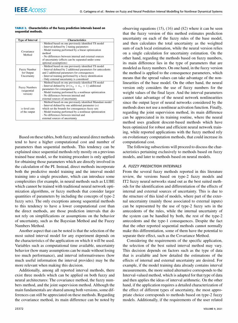
TABLE 2. Characteristics of the fuzzy prediction intervals based onsequential methods.
Based on these tables, both fuzzy and neural direct methodstend to have a higher computational cost and number ofparameters than sequential methods. This tendency can beexplained since sequential methods rely mostly on a previoustrained base model, so the training procedure is only appliedfor obtaining those parameters which are directly involved inthe calculation of the PI. Instead, direct methods incorporateboth the predictive model training and the interval modeltraining into a single procedure, which can introduce somecomplexities (for example, in neural methods such as LUBEwhich cannot be trained with traditional neural network opti-mization algorithms, or fuzzy methods that consider largerquantities of parameters by including the concepts of type-2fuzzy sets). The only exceptions among sequential methodsto this tendency to have a lower computational cost thanthe direct methods, are those prediction intervals that donot rely on simplifications or assumptions on the behaviorof uncertainty, such as the Bayesian Method and the FuzzyNumbers Method.
Another aspect that can be noted is that the selection of themost suited interval model for any experiment depends onthe characteristics of the application on which it will be used.Variables such as computational time available, uncertaintybehavior (howmany assumptions can be made without losingtoo much performance), and interval informativeness (howmuch useful information the interval provides) may be themore relevant when making this decision.
Additionally, among all reported interval methods, thereexist three models which can be applied on both fuzzy andneural architectures: The covariance method, the fuzzy num-bers method, and the joint supervision method. Although themain fundamentals are shared among both versions, some dif-ferences can still be appreciated on these methods. Regardingthe covariance method, its main difference can be noted by
observing equations (15), (16) and (82) where it can be seenthat the fuzzy version of this method estimates predictionuncertainty on each of the fuzzy rules of the base model,and then calculates the total uncertainty as the weightedsum of each local estimation, while the neural version relieson a single calculation for uncertainty estimation. On theother hand, regarding the methods based on fuzzy numbers,its main difference lies in the type of parameters that aremodeled as fuzzy numbers. On one hand, in the fuzzy versionthe method is applied to the consequence parameters, whichmeans that the spread values can take advantage of the non-linearities of the base model. On the other hand, the neuralversion only considers the use of fuzzy numbers for theweight values of the final layer. And the interval parameterscannot take advantage of the neural network nonlinearitiessince the output layer of neural networks considered by themethods does not use a nonlinear activation function. Finally,regarding the joint supervision method, its main differencecan be appreciated in its training routine, where the neuralmethod uses gradient descent-based methods which havebeen optimized for robust and efficient neural network train-ing, while reported applications with the fuzzy method relyon evolutionary computation methods, that could increase itscomputational cost.
The following subsections will proceed to discuss the char-acteristics pertaining exclusively to methods based on fuzzymodels, and later to methods based on neural models.
A. FUZZY PREDICTION INTERVALSFrom the several fuzzy methods reported in this literaturereview, the versions based on type-2 fuzzy models andIT2 fuzzy neural networks stand out as the best suited meth-ods for the identification and differentiation of the effects ofinternal and external sources of uncertainty. This is due tothe structure of this kind of models, where part of the exter-nal uncertainty (mainly those associated to external inputs)can be represented by the use of type-2 fuzzy sets in theantecedents of the rules, while the internal uncertainty ofthe system can be handled by both, the rest of the type-2antecedents and the type-1 consequences. Despite the factthat the other reported sequential methods cannot normallymake this differentiation, some of them have the potential toseparate their effect, such as the Covariance Method.
Considering the requirements of the specific application,the selection of the best suited interval method may vary.This decision depends on factors such as the type of datathat is available and how detailed the estimations of theeffects of internal and external uncertainty are desired. Forexample, if the model training data already contains intervalmeasurements, the more suited alternative corresponds to theInterval-valued method, which is adapted for that type of dataand then applies the ideas of interval arithmetic. On the otherhand, if the application requires a detailed characterization ofthe effect of different types of uncertainty, the most appro-priate choice corresponds to methods based on type-2 fuzzymodels. Additionally, if the requirements of the user related
23372 VOLUME 9, 2021
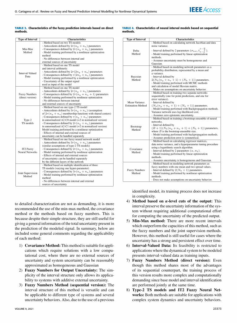
O. Cartagena et al.: Review on Fuzzy and Neural Prediction Interval Modelling for Nonlinear Dynamical Systems
TABLE 3. Characteristics of the fuzzy prediction intervals based on directmethods.
to detailed characterization are not as demanding, it is morerecommended the use of the min-max method, the covariancemethod or the methods based on fuzzy numbers. This isbecause despite their simple structure, they are still useful forgiving a general information of the total uncertainty present inthe prediction of the modeled signal. In summary, below areincluded some general comments regarding the applicabilityof each method:
1) CovarianceMethod:Thismethod is suitable for appli-cations which require solutions with a low compu-tational cost, where there are no external sources ofuncertainty and system uncertainty can be reasonablyapproximated as homogeneous and Gaussian
2) Fuzzy Numbers for Output Uncertainty: The sim-plicity of the interval structure only allows its applica-bility to systems with additive external uncertainty.
3) Fuzzy Numbers Method (sequential version): Theinterval structure of this method is versatile and canbe applicable to different type of systems and severaluncertainty behaviors. Also, due to the use of a previous
TABLE 4. Characteristics of neural interval models based on sequentialmethods.
identified model, its training process does not increasein complexity.
4) Method based on α-level cuts of the output: Thisinterval preserve the uncertainty information of the sys-tem without requiring additional computational effortfor computing the uncertainty of the predicted output.
5) Min-Max method: There are more recent intervalswhich outperform the capacities of this method, such asthe fuzzy numbers and the joint supervision methods.However, this method is still useful for cases where theuncertainty has a strong and persistent effect over time.
6) Interval-Valued Data: Its feasibility is restricted toapplicationswhere the dynamical system to bemodeledpresents interval-valued data as training inputs.
7) Fuzzy Numbers Method (direct version): Eventhough this method shares most of the advantagesof its sequential counterpart, the training process ofthis version results more complex and computationallydemanding since base model and interval identificationare performed jointly at the same time.
8) Type-2 TS models and IT2 Fuzzy Neural Net-works:Both methods are suitable for applications withcomplex system dynamics and uncertainty behaviors.
VOLUME 9, 2021 23373
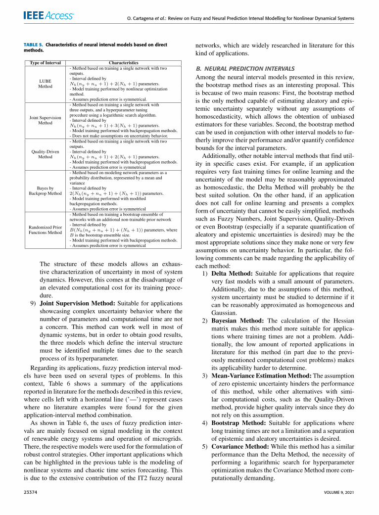
O. Cartagena et al.: Review on Fuzzy and Neural Prediction Interval Modelling for Nonlinear Dynamical Systems
TABLE 5. Characteristics of neural interval models based on directmethods.
The structure of these models allows an exhaus-tive characterization of uncertainty in most of systemdynamics. However, this comes at the disadvantage ofan elevated computational cost for its training proce-dure.
9) Joint Supervision Method: Suitable for applicationsshowcasing complex uncertainty behavior where thenumber of parameters and computational time are nota concern. This method can work well in most ofdynamic systems, but in order to obtain good results,the three models which define the interval structuremust be identified multiple times due to the searchprocess of its hyperparameter.
Regarding its applications, fuzzy prediction interval mod-els have been used on several types of problems. In thiscontext, Table 6 shows a summary of the applicationsreported in literature for the methods described in this review,where cells left with a horizontal line (’—’) represent caseswhere no literature examples were found for the givenapplication-interval method combination.
As shown in Table 6, the uses of fuzzy prediction inter-vals are mainly focused on signal modeling in the contextof renewable energy systems and operation of microgrids.There, the respective models were used for the formulation ofrobust control strategies. Other important applications whichcan be highlighted in the previous table is the modeling ofnonlinear systems and chaotic time series forecasting. Thisis due to the extensive contribution of the IT2 fuzzy neural
networks, which are widely researched in literature for thiskind of applications.
B. NEURAL PREDICTION INTERVALSAmong the neural interval models presented in this review,the bootstrap method rises as an interesting proposal. Thisis because of two main reasons: First, the bootstrap methodis the only method capable of estimating aleatory and epis-temic uncertainty separately without any assumptions ofhomoscedasticity, which allows the obtention of unbiasedestimators for these variables. Second, the bootstrap methodcan be used in conjunction with other interval models to fur-therly improve their performance and/or quantify confidencebounds for the interval parameters.
Additionally, other notable interval methods that find util-ity in specific cases exist. For example, if an applicationrequires very fast training times for online learning and theuncertainty of the model may be reasonably approximatedas homoscedastic, the Delta Method will probably be thebest suited solution. On the other hand, if an applicationdoes not call for online learning and presents a complexform of uncertainty that cannot be easily simplified, methodssuch as Fuzzy Numbers, Joint Supervision, Quality-Drivenor even Bootstrap (especially if a separate quantification ofaleatory and epistemic uncertainties is desired) may be themost appropriate solutions since they make none or very fewassumptions on uncertainty behavior. In particular, the fol-lowing comments can be made regarding the applicability ofeach method:
1) Delta Method: Suitable for applications that requirevery fast models with a small amount of parameters.Additionally, due to the assumptions of this method,system uncertainty must be studied to determine if itcan be reasonably approximated as homogeneous andGaussian.
2) Bayesian Method: The calculation of the Hessianmatrix makes this method more suitable for applica-tions where training times are not a problem. Addi-tionally, the low amount of reported applications inliterature for this method (in part due to the previ-ously mentioned computational cost problems) makesits applicability harder to determine.
3) Mean-Variance EstimationMethod: The assumptionof zero epistemic uncertainty hinders the performanceof this method, while other alternatives with simi-lar computational costs, such as the Quality-Drivenmethod, provide higher quality intervals since they donot rely on this assumption.
4) Bootstrap Method: Suitable for applications wherelong training times are not a limitation and a separationof epistemic and aleatory uncertainties is desired.
5) Covariance Method: While this method has a similarperformance than the Delta Method, the necessity ofperforming a logarithmic search for hyperparameteroptimization makes the Covariance Method more com-putationally demanding.
23374 VOLUME 9, 2021
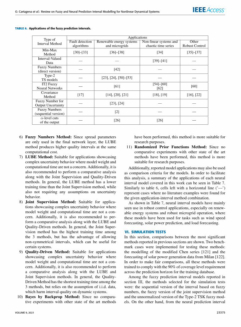
O. Cartagena et al.: Review on Fuzzy and Neural Prediction Interval Modelling for Nonlinear Dynamical Systems
TABLE 6. Applications of the fuzzy prediction intervals.
6) Fuzzy Numbers Method: Since spread parametersare only used in the final network layer, the LUBEmethod produces higher quality intervals at the samecomputational cost.
7) LUBE Method: Suitable for applications showcasingcomplex uncertainty behavior where model weight andcomputational time are not a concern. Additionally, it isalso recommended to perform a comparative analysisalong with the Joint Supervision and Quality-Drivenmethods. In general, the LUBE method has a lowertraining time than the Joint Supervision method, whilealso not requiring any assumptions on uncertaintybehavior.
8) Joint Supervision Method: Suitable for applica-tions showcasing complex uncertainty behavior wheremodel weight and computational time are not a con-cern. Additionally, it is also recommended to per-form a comparative analysis along with the LUBE andQuality-Driven methods. In general, the Joint Super-vision method has the highest training time amongthe 3 methods, but has the advantage of allowingnon-symmetrical intervals, which can be useful forcertain systems.
9) Quality-Driven Method: Suitable for applicationsshowcasing complex uncertainty behavior wheremodel weight and computational time are not a con-cern. Additionally, it is also recommended to performa comparative analysis along with the LUBE andJoint Supervision methods. In general, the Quality-DrivenMethod has the shortest training time among the3 methods, but relies on the assumption of i.i.d. data,which harm interval quality on dynamic systems.
10) Bayes by Backprop Method: Since no compara-tive experiments with other state of the art methods
have been performed, this method is more suitable forresearch purposes.
11) Randomized Prior Functions Method: Since nocomparative experiments with other state of the artmethods have been performed, this method is moresuitable for research purposes.
Additionally, reportedmodel applicationsmay also be usedas comparison criteria for the models. In order to facilitatethis analysis, a summary of the applications of each neuralinterval model covered in this work can be seen in Table 7.Similarly to table 6, cells left with a horizontal line (’—’)represent cases where no literature examples were found forthe given application-interval method combination.
As shown in Table 7, neural interval models have mainlyseen use in robust control applications, especially on renew-able energy systems and robust microgrid operation, wherethese models have been used for tasks such as wind speedforecasting, solar power prediction, and load forecasting.
VI. SIMULATION TESTSIn this section, comparisons between the most significantmethods reported in previous sections are shown. Two bench-mark cases were implemented for testing these methods:the modelling of the modified Chen series [121] and theforecasting of solar power generation data from Milan [122].In order to make fair comparisons, all these methods weretrained to comply with the 90% of coverage level requirementacross the prediction horizon for the training database.
Among the fuzzy prediction interval models reported insection III, the methods selected for the simulation testswere: the sequential version of the interval based on fuzzynumbers, the fuzzy version of the joint supervision methodand the unnormalized version of the Type-2 TSK fuzzy mod-els. On the other hand, from the neural prediction interval
VOLUME 9, 2021 23375
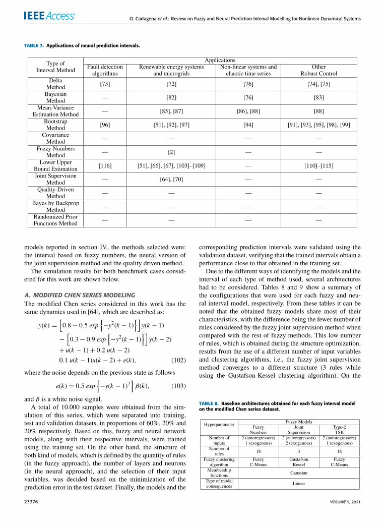
O. Cartagena et al.: Review on Fuzzy and Neural Prediction Interval Modelling for Nonlinear Dynamical Systems
TABLE 7. Applications of neural prediction intervals.
models reported in section IV, the methods selected were:the interval based on fuzzy numbers, the neural version ofthe joint supervision method and the quality driven method.
The simulation results for both benchmark cases consid-ered for this work are shown below.
A. MODIFIED CHEN SERIES MODELINGThe modified Chen series considered in this work has thesame dynamics used in [64], which are described as:
y(k) =[0.8− 0.5 exp
{−y2(k − 1)
}]y(k − 1)
−
[0.3− 0.9 exp
{−y2(k − 1)
}]y(k − 2)
+ u(k − 1)+ 0.2 u(k − 2)
0.1 u(k − 1)u(k − 2)+ e(k), (102)
where the noise depends on the previous state as follows
e(k) = 0.5 exp{−y(k − 1)2
}β(k), (103)
and β is a white noise signal.A total of 10.000 samples were obtained from the sim-
ulation of this series, which were separated into training,test and validation datasets, in proportions of 60%, 20% and20% respectively. Based on this, fuzzy and neural networkmodels, along with their respective intervals, were trainedusing the training set. On the other hand, the structure ofboth kind of models, which is defined by the quantity of rules(in the fuzzy approach), the number of layers and neurons(in the neural approach), and the selection of their inputvariables, was decided based on the minimization of theprediction error in the test dataset. Finally, the models and the
corresponding prediction intervals were validated using thevalidation dataset, verifying that the trained intervals obtain aperformance close to that obtained in the training set.
Due to the different ways of identifying the models and theinterval of each type of method used, several architectureshad to be considered. Tables 8 and 9 show a summary ofthe configurations that were used for each fuzzy and neu-ral interval model, respectively. From these tables it can benoted that the obtained fuzzy models share most of theircharacteristics, with the difference being the fewer number ofrules considered by the fuzzy joint supervision method whencompared with the rest of fuzzy methods. This low numberof rules, which is obtained during the structure optimization,results from the use of a different number of input variablesand clustering algorithms, i.e., the fuzzy joint supervisionmethod converges to a different structure (3 rules whileusing the Gustafson-Kessel clustering algorithm). On the
TABLE 8. Baseline architectures obtained for each fuzzy interval modelon the modified Chen series dataset.
23376 VOLUME 9, 2021
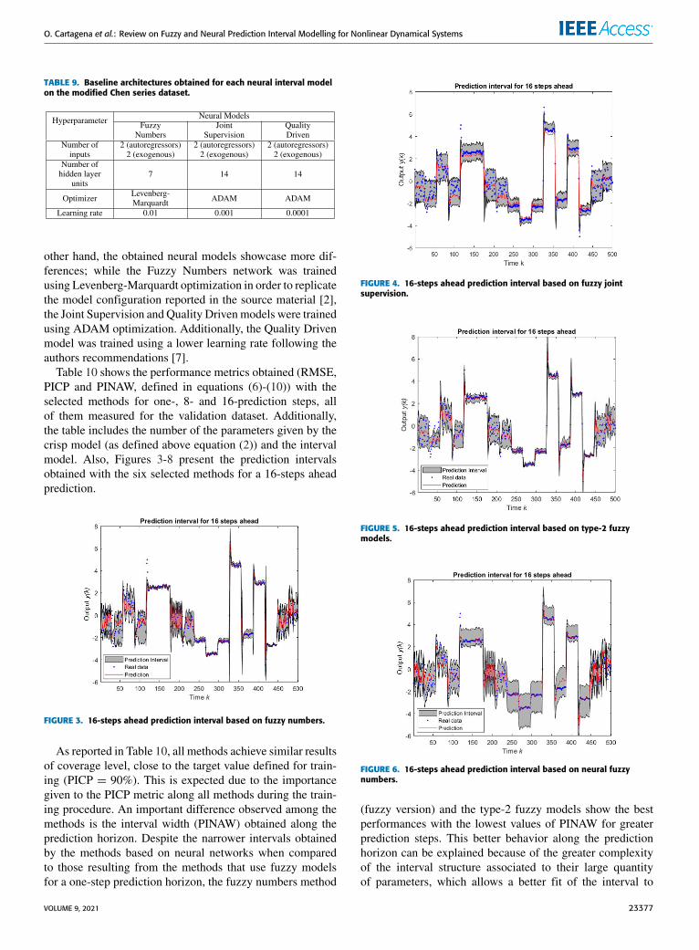
O. Cartagena et al.: Review on Fuzzy and Neural Prediction Interval Modelling for Nonlinear Dynamical Systems
TABLE 9. Baseline architectures obtained for each neural interval modelon the modified Chen series dataset.
other hand, the obtained neural models showcase more dif-ferences; while the Fuzzy Numbers network was trainedusing Levenberg-Marquardt optimization in order to replicatethe model configuration reported in the source material [2],the Joint Supervision and Quality Drivenmodels were trainedusing ADAM optimization. Additionally, the Quality Drivenmodel was trained using a lower learning rate following theauthors recommendations [7].
Table 10 shows the performance metrics obtained (RMSE,PICP and PINAW, defined in equations (6)-(10)) with theselected methods for one-, 8- and 16-prediction steps, allof them measured for the validation dataset. Additionally,the table includes the number of the parameters given by thecrisp model (as defined above equation (2)) and the intervalmodel. Also, Figures 3-8 present the prediction intervalsobtained with the six selected methods for a 16-steps aheadprediction.
FIGURE 3. 16-steps ahead prediction interval based on fuzzy numbers.
As reported in Table 10, all methods achieve similar resultsof coverage level, close to the target value defined for train-ing (PICP = 90%). This is expected due to the importancegiven to the PICP metric along all methods during the train-ing procedure. An important difference observed among themethods is the interval width (PINAW) obtained along theprediction horizon. Despite the narrower intervals obtainedby the methods based on neural networks when comparedto those resulting from the methods that use fuzzy modelsfor a one-step prediction horizon, the fuzzy numbers method
FIGURE 4. 16-steps ahead prediction interval based on fuzzy jointsupervision.
FIGURE 5. 16-steps ahead prediction interval based on type-2 fuzzymodels.
FIGURE 6. 16-steps ahead prediction interval based on neural fuzzynumbers.
(fuzzy version) and the type-2 fuzzy models show the bestperformances with the lowest values of PINAW for greaterprediction steps. This better behavior along the predictionhorizon can be explained because of the greater complexityof the interval structure associated to their large quantityof parameters, which allows a better fit of the interval to
VOLUME 9, 2021 23377
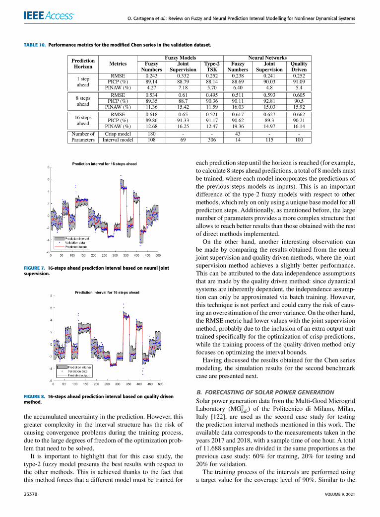
O. Cartagena et al.: Review on Fuzzy and Neural Prediction Interval Modelling for Nonlinear Dynamical Systems
TABLE 10. Performance metrics for the modified Chen series in the validation dataset.
FIGURE 7. 16-steps ahead prediction interval based on neural jointsupervision.
FIGURE 8. 16-steps ahead prediction interval based on quality drivenmethod.
the accumulated uncertainty in the prediction. However, thisgreater complexity in the interval structure has the risk ofcausing convergence problems during the training process,due to the large degrees of freedom of the optimization prob-lem that need to be solved.
It is important to highlight that for this case study, thetype-2 fuzzy model presents the best results with respect tothe other methods. This is achieved thanks to the fact thatthis method forces that a different model must be trained for
each prediction step until the horizon is reached (for example,to calculate 8 steps ahead predictions, a total of 8models mustbe trained, where each model incorporates the predictions ofthe previous steps models as inputs). This is an importantdifference of the type-2 fuzzy models with respect to othermethods, which rely on only using a unique base model for allprediction steps. Additionally, as mentioned before, the largenumber of parameters provides a more complex structure thatallows to reach better results than those obtained with the restof direct methods implemented.
On the other hand, another interesting observation canbe made by comparing the results obtained from the neuraljoint supervision and quality driven methods, where the jointsupervision method achieves a slightly better performance.This can be attributed to the data independence assumptionsthat are made by the quality driven method: since dynamicalsystems are inherently dependent, the independence assump-tion can only be approximated via batch training. However,this technique is not perfect and could carry the risk of caus-ing an overestimation of the error variance. On the other hand,the RMSE metric had lower values with the joint supervisionmethod, probably due to the inclusion of an extra output unittrained specifically for the optimization of crisp predictions,while the training process of the quality driven method onlyfocuses on optimizing the interval bounds.
Having discussed the results obtained for the Chen seriesmodeling, the simulation results for the second benchmarkcase are presented next.
B. FORECASTING OF SOLAR POWER GENERATIONSolar power generation data from the Multi-Good MicrogridLaboratory (MG2
lab) of the Politecnico di Milano, Milan,Italy [122], are used as the second case study for testingthe prediction interval methods mentioned in this work. Theavailable data corresponds to the measurements taken in theyears 2017 and 2018, with a sample time of one hour. A totalof 11.688 samples are divided in the same proportions as theprevious case study: 60% for training, 20% for testing and20% for validation.
The training process of the intervals are performed usinga target value for the coverage level of 90%. Similar to the
23378 VOLUME 9, 2021
O. Cartagena et al.: Review on Fuzzy and Neural Prediction Interval Modelling for Nonlinear Dynamical Systems
Chen series experiment, the structure optimization ofthe models was decided based on the configuration that hadthe best performance of the metrics in the test dataset. A totalof 48 regressors, corresponding to the data of two previousdays, were used as the initial candidate inputs, selecting themost relevant inputs by performing a sensitivity analysis.
Tables 11 and 12 show a summary of the different baselineconfigurations that were obtained for each fuzzy and neuralinterval model, respectively.
TABLE 11. Baseline architectures obtained for each fuzzy interval model.
TABLE 12. Baseline architectures obtained for each neural interval model.
From tables 11 and 12, it can be noted that, unlike theprevious case of the modified Chen series experiment, in thiscase all fuzzy models reported on Table 11 share the samehyperparameters. This is because this time the same numberof input variables and clustering algorithmswere used. On theother hand, the neural models reported on Table 12 preservedmost of their hyperparameters that were used on the case ofthe modified Chen series experiment.
Table 13, shows the performance metrics obtained withthe selected methods for different prediction horizons, allof them measured on the validation dataset. Additionally,Figures 9-14 present the prediction intervals obtained withthe selected methods for a 24 hours ahead prediction.
From Table 13, similar tendencies can be appreciated onsome models when compared to the results obtained for theChen series modeling. In these results, all methods managedto comply with the desired coverage level (PICP) of 90%,while the fuzzy prediction intervals based on fuzzy numbers,the type-2models and the quality drivenmethod presented theoverall narrowest intervals throughout the prediction horizon(see PINAW in Table 13). Additionally, from Figures 9-12 it
FIGURE 9. 24-steps ahead prediction interval based on fuzzy numbers.
FIGURE 10. 24-steps ahead prediction interval based on fuzzy jointsupervision.
FIGURE 11. 24-steps ahead prediction interval based on type-2 fuzzymodels.
can be seen that the fuzzy prediction interval based on fuzzynumbers presents a smoother behavior throughout the plotteddata.
Since the explanation of the main tendencies presented bythe intervals were already covered in the previous benchmarkcase, here the discussion will be focused on those results thatdid not follow these previous trends.
VOLUME 9, 2021 23379
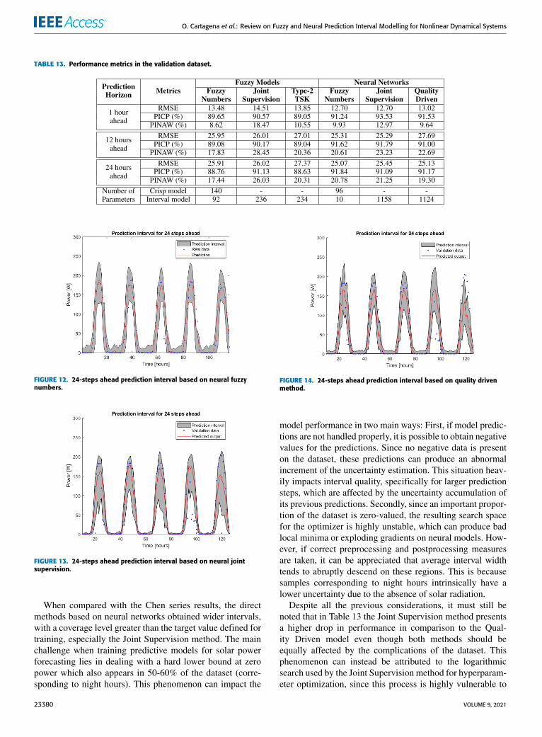
O. Cartagena et al.: Review on Fuzzy and Neural Prediction Interval Modelling for Nonlinear Dynamical Systems
TABLE 13. Performance metrics in the validation dataset.
FIGURE 12. 24-steps ahead prediction interval based on neural fuzzynumbers.
FIGURE 13. 24-steps ahead prediction interval based on neural jointsupervision.
When compared with the Chen series results, the directmethods based on neural networks obtained wider intervals,with a coverage level greater than the target value defined fortraining, especially the Joint Supervision method. The mainchallenge when training predictive models for solar powerforecasting lies in dealing with a hard lower bound at zeropower which also appears in 50-60% of the dataset (corre-sponding to night hours). This phenomenon can impact the
FIGURE 14. 24-steps ahead prediction interval based on quality drivenmethod.
model performance in two main ways: First, if model predic-tions are not handled properly, it is possible to obtain negativevalues for the predictions. Since no negative data is presenton the dataset, these predictions can produce an abnormalincrement of the uncertainty estimation. This situation heav-ily impacts interval quality, specifically for larger predictionsteps, which are affected by the uncertainty accumulation ofits previous predictions. Secondly, since an important propor-tion of the dataset is zero-valued, the resulting search spacefor the optimizer is highly unstable, which can produce badlocal minima or exploding gradients on neural models. How-ever, if correct preprocessing and postprocessing measuresare taken, it can be appreciated that average interval widthtends to abruptly descend on these regions. This is becausesamples corresponding to night hours intrinsically have alower uncertainty due to the absence of solar radiation.
Despite all the previous considerations, it must still benoted that in Table 13 the Joint Supervision method presentsa higher drop in performance in comparison to the Qual-ity Driven model even though both methods should beequally affected by the complications of the dataset. Thisphenomenon can instead be attributed to the logarithmicsearch used by the Joint Supervision method for hyperparam-eter optimization, since this process is highly vulnerable to
23380 VOLUME 9, 2021
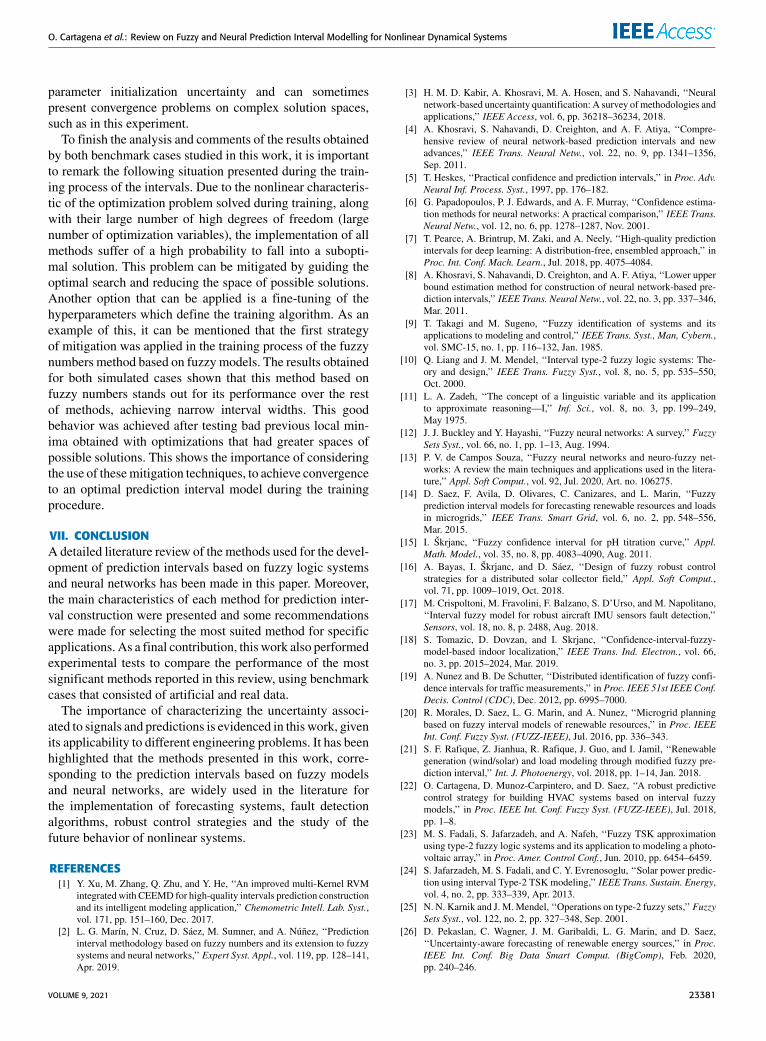
O. Cartagena et al.: Review on Fuzzy and Neural Prediction Interval Modelling for Nonlinear Dynamical Systems
parameter initialization uncertainty and can sometimespresent convergence problems on complex solution spaces,such as in this experiment.
To finish the analysis and comments of the results obtainedby both benchmark cases studied in this work, it is importantto remark the following situation presented during the train-ing process of the intervals. Due to the nonlinear characteris-tic of the optimization problem solved during training, alongwith their large number of high degrees of freedom (largenumber of optimization variables), the implementation of allmethods suffer of a high probability to fall into a subopti-mal solution. This problem can be mitigated by guiding theoptimal search and reducing the space of possible solutions.Another option that can be applied is a fine-tuning of thehyperparameters which define the training algorithm. As anexample of this, it can be mentioned that the first strategyof mitigation was applied in the training process of the fuzzynumbers method based on fuzzy models. The results obtainedfor both simulated cases shown that this method based onfuzzy numbers stands out for its performance over the restof methods, achieving narrow interval widths. This goodbehavior was achieved after testing bad previous local min-ima obtained with optimizations that had greater spaces ofpossible solutions. This shows the importance of consideringthe use of thesemitigation techniques, to achieve convergenceto an optimal prediction interval model during the trainingprocedure.
VII. CONCLUSIONA detailed literature review of the methods used for the devel-opment of prediction intervals based on fuzzy logic systemsand neural networks has been made in this paper. Moreover,the main characteristics of each method for prediction inter-val construction were presented and some recommendationswere made for selecting the most suited method for specificapplications. As a final contribution, this work also performedexperimental tests to compare the performance of the mostsignificant methods reported in this review, using benchmarkcases that consisted of artificial and real data.
The importance of characterizing the uncertainty associ-ated to signals and predictions is evidenced in this work, givenits applicability to different engineering problems. It has beenhighlighted that the methods presented in this work, corre-sponding to the prediction intervals based on fuzzy modelsand neural networks, are widely used in the literature forthe implementation of forecasting systems, fault detectionalgorithms, robust control strategies and the study of thefuture behavior of nonlinear systems.
REFERENCES[1] Y. Xu, M. Zhang, Q. Zhu, and Y. He, ‘‘An improved multi-Kernel RVM
integrated with CEEMD for high-quality intervals prediction constructionand its intelligent modeling application,’’ Chemometric Intell. Lab. Syst.,vol. 171, pp. 151–160, Dec. 2017.
[2] L. G. Marín, N. Cruz, D. Sáez, M. Sumner, and A. Núñez, ‘‘Predictioninterval methodology based on fuzzy numbers and its extension to fuzzysystems and neural networks,’’ Expert Syst. Appl., vol. 119, pp. 128–141,Apr. 2019.
[3] H. M. D. Kabir, A. Khosravi, M. A. Hosen, and S. Nahavandi, ‘‘Neuralnetwork-based uncertainty quantification: A survey of methodologies andapplications,’’ IEEE Access, vol. 6, pp. 36218–36234, 2018.
[4] A. Khosravi, S. Nahavandi, D. Creighton, and A. F. Atiya, ‘‘Compre-hensive review of neural network-based prediction intervals and newadvances,’’ IEEE Trans. Neural Netw., vol. 22, no. 9, pp. 1341–1356,Sep. 2011.
[5] T. Heskes, ‘‘Practical confidence and prediction intervals,’’ in Proc. Adv.Neural Inf. Process. Syst., 1997, pp. 176–182.
[6] G. Papadopoulos, P. J. Edwards, and A. F. Murray, ‘‘Confidence estima-tion methods for neural networks: A practical comparison,’’ IEEE Trans.Neural Netw., vol. 12, no. 6, pp. 1278–1287, Nov. 2001.
[7] T. Pearce, A. Brintrup, M. Zaki, and A. Neely, ‘‘High-quality predictionintervals for deep learning: A distribution-free, ensembled approach,’’ inProc. Int. Conf. Mach. Learn., Jul. 2018, pp. 4075–4084.
[8] A. Khosravi, S. Nahavandi, D. Creighton, and A. F. Atiya, ‘‘Lower upperbound estimation method for construction of neural network-based pre-diction intervals,’’ IEEE Trans. Neural Netw., vol. 22, no. 3, pp. 337–346,Mar. 2011.
[9] T. Takagi and M. Sugeno, ‘‘Fuzzy identification of systems and itsapplications to modeling and control,’’ IEEE Trans. Syst., Man, Cybern.,vol. SMC-15, no. 1, pp. 116–132, Jan. 1985.
[10] Q. Liang and J. M. Mendel, ‘‘Interval type-2 fuzzy logic systems: The-ory and design,’’ IEEE Trans. Fuzzy Syst., vol. 8, no. 5, pp. 535–550,Oct. 2000.
[11] L. A. Zadeh, ‘‘The concept of a linguistic variable and its applicationto approximate reasoning—I,’’ Inf. Sci., vol. 8, no. 3, pp. 199–249,May 1975.
[12] J. J. Buckley and Y. Hayashi, ‘‘Fuzzy neural networks: A survey,’’ FuzzySets Syst., vol. 66, no. 1, pp. 1–13, Aug. 1994.
[13] P. V. de Campos Souza, ‘‘Fuzzy neural networks and neuro-fuzzy net-works: A review the main techniques and applications used in the litera-ture,’’ Appl. Soft Comput., vol. 92, Jul. 2020, Art. no. 106275.
[14] D. Saez, F. Avila, D. Olivares, C. Canizares, and L. Marin, ‘‘Fuzzyprediction interval models for forecasting renewable resources and loadsin microgrids,’’ IEEE Trans. Smart Grid, vol. 6, no. 2, pp. 548–556,Mar. 2015.
[15] I. Škrjanc, ‘‘Fuzzy confidence interval for pH titration curve,’’ Appl.Math. Model., vol. 35, no. 8, pp. 4083–4090, Aug. 2011.
[16] A. Bayas, I. Škrjanc, and D. Sáez, ‘‘Design of fuzzy robust controlstrategies for a distributed solar collector field,’’ Appl. Soft Comput.,vol. 71, pp. 1009–1019, Oct. 2018.
[17] M. Crispoltoni, M. Fravolini, F. Balzano, S. D’Urso, and M. Napolitano,‘‘Interval fuzzy model for robust aircraft IMU sensors fault detection,’’Sensors, vol. 18, no. 8, p. 2488, Aug. 2018.
[18] S. Tomazic, D. Dovzan, and I. Skrjanc, ‘‘Confidence-interval-fuzzy-model-based indoor localization,’’ IEEE Trans. Ind. Electron., vol. 66,no. 3, pp. 2015–2024, Mar. 2019.
[19] A. Nunez and B. De Schutter, ‘‘Distributed identification of fuzzy confi-dence intervals for traffic measurements,’’ in Proc. IEEE 51st IEEE Conf.Decis. Control (CDC), Dec. 2012, pp. 6995–7000.
[20] R. Morales, D. Saez, L. G. Marin, and A. Nunez, ‘‘Microgrid planningbased on fuzzy interval models of renewable resources,’’ in Proc. IEEEInt. Conf. Fuzzy Syst. (FUZZ-IEEE), Jul. 2016, pp. 336–343.
[21] S. F. Rafique, Z. Jianhua, R. Rafique, J. Guo, and I. Jamil, ‘‘Renewablegeneration (wind/solar) and load modeling through modified fuzzy pre-diction interval,’’ Int. J. Photoenergy, vol. 2018, pp. 1–14, Jan. 2018.
[22] O. Cartagena, D. Munoz-Carpintero, and D. Saez, ‘‘A robust predictivecontrol strategy for building HVAC systems based on interval fuzzymodels,’’ in Proc. IEEE Int. Conf. Fuzzy Syst. (FUZZ-IEEE), Jul. 2018,pp. 1–8.
[23] M. S. Fadali, S. Jafarzadeh, and A. Nafeh, ‘‘Fuzzy TSK approximationusing type-2 fuzzy logic systems and its application to modeling a photo-voltaic array,’’ in Proc. Amer. Control Conf., Jun. 2010, pp. 6454–6459.
[24] S. Jafarzadeh, M. S. Fadali, and C. Y. Evrenosoglu, ‘‘Solar power predic-tion using interval Type-2 TSK modeling,’’ IEEE Trans. Sustain. Energy,vol. 4, no. 2, pp. 333–339, Apr. 2013.
[25] N. N. Karnik and J. M. Mendel, ‘‘Operations on type-2 fuzzy sets,’’ FuzzySets Syst., vol. 122, no. 2, pp. 327–348, Sep. 2001.
[26] D. Pekaslan, C. Wagner, J. M. Garibaldi, L. G. Marin, and D. Saez,‘‘Uncertainty-aware forecasting of renewable energy sources,’’ in Proc.IEEE Int. Conf. Big Data Smart Comput. (BigComp), Feb. 2020,pp. 240–246.
VOLUME 9, 2021 23381
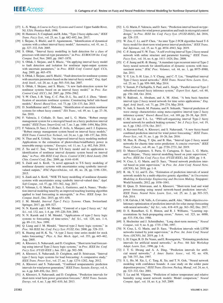
O. Cartagena et al.: Review on Fuzzy and Neural Prediction Interval Modelling for Nonlinear Dynamical Systems
[27] L.-X.Wang, ACourse in Fuzzy Systems and Control. Upper Saddle River,NJ, USA: Prentice-Hall, 1996.
[28] H. Hamrawi, S. Coupland, and R. John, ‘‘Type-2 fuzzy alpha-cuts,’’ IEEETrans. Fuzzy Syst., vol. 25, no. 3, pp. 682–692, Jun. 2017.
[29] I. Škrjanc, S. Blažič, and O. Agamennoni, ‘‘Identification of dynamicalsystems with a robust interval fuzzy model,’’ Automatica, vol. 41, no. 2,pp. 327–332, Feb. 2005.
[30] S. Oblak, ‘‘Interval fuzzy modelling in fault detection for a class ofprocesses with interval-type parameters,’’ in Proc. EUROCON Int. Conf.Comput. Tool, Nov. 2005, pp. 1867–1870.
[31] S. Oblak, I. Skrjanc, and S. Blazic, ‘‘On applying interval fuzzy modelto fault detection and isolation for nonlinear input-output systemswith uncertain parameters,’’ in Proc. IEEE Conf. Control Appl. CCA,Aug. 2005, pp. 465–470.
[32] S. Oblak, I. Škrjanc, and S. Blažič, ‘‘Fault detection for nonlinear systemswith uncertain parameters based on the interval fuzzy model,’’ Eng. Appl.Artif. Intell., vol. 20, no. 4, pp. 503–510, Jun. 2007.
[33] S. Oblak, I. Skrjanc, and S. Blazic, ‘‘A new fault-detection system fornonlinear systems based on an interval fuzzy model,’’ in Proc. Eur.Control Conf. (ECC), Jul. 2007, pp. 2956–2962.
[34] Y.-W. Chen, J.-B. Yang, C.-C. Pan, D.-L. Xu, and Z.-J. Zhou, ‘‘Identi-fication of uncertain nonlinear systems: Constructing belief rule-basedmodels,’’ Knowl.-Based Syst., vol. 73, pp. 124–133, Jan. 2015.
[35] D. Senthilkumar and C. Mahanta, ‘‘Identification of uncertain nonlinearsystems for robust fuzzy control,’’ ISA Trans., vol. 49, no. 1, pp. 27–38,Jan. 2010.
[36] F. Valencia, J. Collado, D. Saez, and L. G. Marin, ‘‘Robust energymanagement system for a microgrid based on a fuzzy prediction intervalmodel,’’ IEEE Trans. Smart Grid, vol. 7, no. 3, pp. 1486–1494,May 2016.
[37] F. Valencia, D. Saez, J. Collado, F. Avila, A. Marquez, and J. J. Espinosa,‘‘Robust energy management system based on interval fuzzy models,’’IEEE Trans. Control Syst. Technol., vol. 24, no. 1, pp. 140–157, Jan. 2016.
[38] N. Thao and K. Uchida, ‘‘An improved interval fuzzy modeling method:Applications to the estimation of photovoltaic/wind/battery power inrenewable energy systems,’’ Energies, vol. 11, no. 3, p. 482, Feb. 2018.
[39] Z. Xu and C. Sun, ‘‘Interval T-S fuzzy model and its application toidentification of nonlinear interval dynamic system based on intervaldata,’’ in Proc. 48h IEEE Conf. Decis. Control (CDC) Held Jointly 28thChin. Control Conf., Dec. 2009, pp. 4144–4149.
[40] S. Zaidi and A. Kroll, ‘‘A novel approach to T-S fuzzy modeling ofnonlinear dynamic systems with uncertainties using symbolic interval-valued outputs,’’ IFAC-PapersOnLine, vol. 48, no. 28, pp. 1196–1201,2015.
[41] S. Zaidi and A. Kroll, ‘‘NOE TS fuzzy modelling of nonlinear dynamicsystems with uncertainties using symbolic interval-valued data,’’ Appl.Soft Comput., vol. 57, pp. 353–362, Aug. 2017.
[42] F. Veltman, L. G. Marin, D. Saez, L. Guitierrez, and A. Nunez, ‘‘Predic-tion interval modeling tuned by an improved teaching learning algorithmapplied to load forecasting in microgrids,’’ in Proc. IEEE Symp. Ser.Comput. Intell., Dec. 2015, pp. 651–658.
[43] J. M. Mendel, Interval Type-2 Fuzzy Systems. Cham, Switzerland:Springer, 2017, pp. 449–527.
[44] N. N. Karnik and J. M. Mendel, ‘‘Centroid of a type-2 fuzzy set,’’ Inf.Sci., vol. 132, nos. 1–4, pp. 195–220, Feb. 2001.
[45] N. N. Karnik and J. M. Mendel, ‘‘Applications of type-2 fuzzy logicsystems to forecasting of time-series,’’ Inf. Sci., vol. 120, nos. 1–4,pp. 89–111, Nov. 1999.
[46] Q. Liang and J. M. Mendel, ‘‘Interval type-2 fuzzy logic systems,’’ inProc. 9th IEEE Int. Conf. Fuzzy Syst. FUZZ, Oct. 2000, pp. 328–333.
[47] K. Huarng and H.-K. Yu, ‘‘A type 2 fuzzy time series model for stockindex forecasting,’’ Phys. A, Stat. Mech. Appl., vol. 353, pp. 445–462,Aug. 2005.
[48] A. Khosravi, S. Nahavandi, and D. Creighton, ‘‘Short term load forecast-ing using interval Type-2 fuzzy logic systems,’’ in Proc. IEEE Int. Conf.Fuzzy Syst. (FUZZ-IEEE ), Jun. 2011, pp. 502–508.
[49] A. Khosravi, S. Nahavandi, D. Creighton, and D. Srinivasan, ‘‘Intervaltype-2 fuzzy logic systems for load forecasting: A comparative study,’’IEEE Trans. Power Syst., vol. 27, no. 3, pp. 1274–1282, Aug. 2012.
[50] A. Khosravi and S. Nahavandi, ‘‘Combined nonparametric predictionintervals for wind power generation,’’ IEEE Trans. Sustain. Energy, vol. 4,no. 4, pp. 849–856, Oct. 2013.
[51] A. Khosravi, S. Nahavandi, and D. Creighton, ‘‘Prediction intervals forshort-term wind farm power generation forecasts,’’ IEEE Trans. Sustain.Energy, vol. 4, no. 3, pp. 602–610, Jul. 2013.
[52] L. G. Marin, F. Valencia, and D. Saez, ‘‘Prediction interval based on type-2 fuzzy systems for wind power generation and loads in microgrid controldesign,’’ in Proc. IEEE Int. Conf. Fuzzy Syst. (FUZZ-IEEE), Jul. 2016,pp. 328–335.
[53] W. Zou, C. Li, and P. Chen, ‘‘An inter Type-2 FCR algorithm based T–Sfuzzy model for short-term wind power interval prediction,’’ IEEE Trans.Ind. Informat., vol. 15, no. 9, pp. 4934–4943, Sep. 2019.
[54] C.-F. Juang andY.-W. Tsao, ‘‘A self-evolving interval Type-2 fuzzy neuralnetwork with online structure and parameter learning,’’ IEEE Trans.Fuzzy Syst., vol. 16, no. 6, pp. 1411–1424, Dec. 2008.
[55] C.-F. Juang and R.-B. Huang, ‘‘Amamdani-type recurrent interval Type-2fuzzy neural network for identification of dynamic systems with mea-surement noise,’’ IFAC Proc. Volumes, vol. 44, no. 1, pp. 8975–8980,Jan. 2011.
[56] Y.-Y. Lin, S.-H. Liao, J.-Y. Chang, and C.-T. Lin, ‘‘Simplified intervalType-2 fuzzy neural networks,’’ IEEE Trans. Neural Netw. Learn. Syst.,vol. 25, no. 5, pp. 959–969, May 2014.
[57] V. Sumati, P. Chellapilla, S. Paul, and L. Singh, ‘‘Parallel interval Type-2subsethood neural fuzzy inference system,’’ Expert Syst. Appl., vol. 60,pp. 156–168, Oct. 2016.
[58] N. Baklouti, A. Abraham, and A. M. Alimi, ‘‘A beta basis functioninterval type-2 fuzzy neural network for time series applications,’’ Eng.Appl. Artif. Intell., vol. 71, pp. 259–274, May 2018.
[59] N. Anh, S. Suresh, M. Pratama, and N. Srikanth, ‘‘Interval prediction ofwave energy characteristics using meta-cognitive interval type-2 fuzzyinference system,’’ Knowl.-Based Syst., vol. 169, pp. 28–38, Apr. 2019.
[60] C.-M. Lin and T.-L. Le, ‘‘PSO-self-organizing interval Type-2 fuzzyneural network for antilock braking systems,’’ Int. J. Fuzzy Syst., vol. 19,no. 5, pp. 1362–1374, Oct. 2017.
[61] A. Kavousi-Fard, A. Khosravi, and S. Nahavandi, ‘‘A new fuzzy-basedcombined prediction interval for wind power forecasting,’’ IEEE Trans.Power Syst., vol. 31, no. 1, pp. 18–26, Jan. 2016.
[62] M. Han, K. Zhong, T. Qiu, and B. Han, ‘‘Interval type-2 fuzzy neuralnetworks for chaotic time series prediction: A concise overview,’’ IEEETrans. Cybern., vol. 49, no. 7, pp. 2720–2731, Jul. 2019.
[63] D. Munoz-Carpintero, S. Parra, O. Cartagena, D. Saez, L. G. Marin,and I. Skrjanc, ‘‘Fuzzy interval modelling based on joint supervision,’’in Proc. IEEE Int. Conf. Fuzzy Syst. (FUZZ-IEEE), Jul. 2020, pp. 1–8.
[64] N. Cruz, L. G. Marin, and D. Saez, ‘‘Neural network prediction inter-val based on joint supervision,’’ in Proc. Int. Joint Conf. Neural Netw.(IJCNN), Jul. 2018, pp. 1–8.
[65] R. Ak, Y. LI, and E. Zio, ‘‘Estimation of prediction intervals of neuralnetwork models by a multi-objective genetic algorithm,’’ in UncertaintyModeling in Knowledge Engineering and Decision Making. Singapore:World Scientific, 2012, pp. 1036–1041.
[66] H. Quan, D. Srinivasan, and A. Khosravi, ‘‘Short-term load and windpower forecasting using neural network-based prediction intervals,’’IEEE Trans. Neural Netw. Learn. Syst., vol. 25, no. 2, pp. 303–315,Feb. 2014.
[67] I.M. Galván, J.M. Valls, A. Cervantes, and R. Aler, ‘‘Multi-objective evo-lutionary optimization of prediction intervals for solar energy forecastingwith neural networks,’’ Inf. Sci., vols. 418–419, pp. 363–382, Dec. 2017.
[68] D. E. Rumelhart, G. E. Hinton, and R. J. Williams, ‘‘Learning rep-resentations by back-propagating errors,’’ Nature, vol. 323, no. 6088,pp. 533–536, Oct. 1986.
[69] S. Hochreiter and J. Schmidhuber, ‘‘Long short-term memory,’’ NeuralComput., vol. 9, no. 8, pp. 1735–1780, 1997.
[70] N. Cruz, L. G. Marin, and D. Saez, ‘‘Prediction intervals with LSTMnetworks trained by joint supervision,’’ in Proc. Int. Joint Conf. NeuralNetw. (IJCNN), Jul. 2019, pp. 1–8.
[71] L. H. Ungar, R. D. De Veaux, and E. Rosengarten, ‘‘Estimating predictionintervals for artificial neural networks,’’ in Proc. 9th Yale WorkshopAdapt. Learn. Syst., 1996, pp. 1–6.
[72] J. T. G. Hwang and A. A. Ding, ‘‘Prediction intervals for artifi-cial neural networks,’’ J. Amer. Statist. Assoc., vol. 92, no. 438,pp. 748–757, Jun. 1997.
[73] S. L. Ho, M. Xie, L. C. Tang, K. Xu, and T. N. Goh, ‘‘Neural networkmodeling with confidence bounds: A case study on the solder pastedeposition process,’’ IEEE Trans. Electron. Packag.Manuf., vol. 24, no. 4,pp. 323–332, Oct. 2001.
[74] T. Lu and M. Viljanen, ‘‘Prediction of indoor temperature and relativehumidity using neural network models: Model comparison,’’ NeuralComput. Appl., vol. 18, no. 4, p. 345, 2009.
23382 VOLUME 9, 2021
O. Cartagena et al.: Review on Fuzzy and Neural Prediction Interval Modelling for Nonlinear Dynamical Systems
[75] Y.-M. Kuo, C.-W. Liu, and K.-H. Lin, ‘‘Evaluation of the ability of anartificial neural network model to assess the variation of groundwaterquality in an area of blackfoot disease in taiwan,’’ Water Res., vol. 38,no. 1, pp. 148–158, Jan. 2004.
[76] A. Khosravi, E. Mazloumi, S. Nahavandi, D. Creighton, andJ. W. C. van Lint, ‘‘Prediction intervals to account for uncertaintiesin travel time prediction,’’ IEEE Trans. Intell. Transp. Syst., vol. 12,no. 2, pp. 537–547, Jun. 2011.
[77] R. D. De VlEAUX, J. Schumi, J. Schweinsberg, and L. H. Ungar, ‘‘Pre-diction intervals for neural networks via nonlinear regression,’’ Techno-metrics, vol. 40, no. 4, pp. 273–282, Nov. 1998.
[78] A. Khosravi, S. Nahavandi, and D. Creighton, ‘‘A prediction interval-based approach to determine optimal structures of neural network meta-models,’’ Expert Syst. Appl., vol. 37, no. 3, pp. 2377–2387, Mar. 2010.
[79] A. Khosravi, S. Nahavandi, and D. Creighton, ‘‘Construction of optimalprediction intervals for load forecasting problems,’’ IEEE Trans. PowerSyst., vol. 25, no. 3, pp. 1496–1503, Aug. 2010.
[80] J. S. Denker and Y. LeCun, ‘‘Transforming neural-net output levels toprobability distributions,’’ in Proc. Adv. Neural Inf. Process. Syst., 1991,pp. 853–859.
[81] D. J. C. MacKay, ‘‘A practical Bayesian framework for backpropagationnetworks,’’ Neural Comput., vol. 4, no. 3, pp. 448–472, May 1992.
[82] A. Khosravi, S. Nahavandi, and D. Creighton, ‘‘Load forecasting andneural networks: A prediction interval-based perspective,’’ in Computa-tional Intelligence in Power Engineering (Studies in Computational Intel-ligence), vol. 302. Berlin, Germany: Springer-Verlag, 2010, pp. 131–150,doi: 10.1007/978-3-642-14013-6_5.
[83] A. F. Torres, W. R. Walker, and M. McKee, ‘‘Forecasting daily potentialevapotranspiration using machine learning and limited climatic data,’’Agricult. Water Manage., vol. 98, no. 4, pp. 553–562, Feb. 2011.
[84] D. A. Nix and A. S. Weigend, ‘‘Estimating the mean and variance of thetarget probability distribution,’’ in Proc. IEEE Int. Conf. Neural Netw.(ICNN), Jun. 1994, pp. 55–60.
[85] A. Khosravi and S. Nahavandi, ‘‘An optimized mean variance estimationmethod for uncertainty quantification of wind power forecasts,’’ Int. J.Electr. Power Energy Syst., vol. 61, pp. 446–454, Oct. 2014.
[86] J.-N. Hwang and E. Little, ‘‘Real time recurrent neural networks for timeseries prediction and confidence estimation,’’ in Proc. Int. Conf. NeuralNetw. (ICNN), Jun. 1996, pp. 1889–1894.
[87] M. Rigamonti, P. Baraldi, E. Zio, I. Roychoudhury, K. Goebel, andS. Poll, ‘‘Ensemble of optimized echo state networks for remaining usefullife prediction,’’ Neurocomputing, vol. 281, pp. 121–138, Mar. 2018.
[88] W. Yao, Z. Zeng, and C. Lian, ‘‘Generating probabilistic predictions usingmean-variance estimation and echo state network,’’ Neurocomputing,vol. 219, pp. 536–547, Jan. 2017.
[89] G. Paass, ‘‘Assessing and improving neural network predictions by thebootstrap algorithm,’’ in Proc. Adv. Neural Inf. Process. Syst., 1993,pp. 196–203.
[90] Z.-H. Zhou, J. Wu, and W. Tang, ‘‘Ensembling neural networks: Manycould be better than all,’’ Artif. Intell., vol. 137, nos. 1–2, pp. 239–263,May 2002.
[91] M. R. A. van Gent, H. F. P. van den Boogaard, B. Pozueta, andJ. R. Medina, ‘‘Neural network modelling of wave overtopping at coastalstructures,’’ Coastal Eng., vol. 54, no. 8, pp. 586–593, Aug. 2007.
[92] P. Pinson and G. Kariniotakis, ‘‘On-line assessment of prediction riskfor wind power production forecasts,’’ Wind Energy, vol. 7, no. 2,pp. 119–132, Apr. 2004.
[93] M. Talebizadeh andA.Moridnejad, ‘‘Uncertainty analysis for the forecastof lake level fluctuations using ensembles of ANN and ANFIS models,’’Expert Syst. Appl., vol. 38, no. 4, pp. 4126–4135, Apr. 2011.
[94] E.Mazloumi, G. Rose, G. Currie, and S.Moridpour, ‘‘Prediction intervalsto account for uncertainties in neural network predictions: Methodologyand application in bus travel time prediction,’’ Eng. Appl. Artif. Intell.,vol. 24, no. 3, pp. 534–542, Apr. 2011.
[95] E. Zio, ‘‘A study of the bootstrap method for estimating the accuracy ofartificial neural networks in predicting nuclear transient processes,’’ IEEETrans. Nucl. Sci., vol. 53, no. 3, pp. 1460–1478, Jun. 2006.
[96] P. Baraldi, M. Compare, S. Sauco, and E. Zio, ‘‘Ensemble neural network-based particle filtering for prognostics,’’ Mech. Syst. Signal Process.,vol. 41, nos. 1–2, pp. 288–300, Dec. 2013.
[97] A. Khosravi, S. Nahavandi, and D. Creighton, ‘‘Quantifying uncertain-ties of neural network-based electricity price forecasts,’’ Appl. Energy,vol. 112, pp. 120–129, Dec. 2013.
[98] B. D. Conduit, N. G. Jones, H. J. Stone, and G. J. Conduit, ‘‘Design of anickel-base superalloy using a neural network,’’Mater. Design, vol. 131,pp. 358–365, Oct. 2017.
[99] K. Ristovski, S. Vucetic, and Z. Obradovic, ‘‘Uncertainty analysis ofNeural-Network-Based aerosol retrieval,’’ IEEE Trans. Geosci. RemoteSens., vol. 50, no. 2, pp. 409–414, Feb. 2012.
[100] J. G. Carney, P. Cunningham, and U. Bhagwan, ‘‘Confidence and predic-tion intervals for neural network ensembles,’’ in Proc. IJCNN Int. JointConf. Neural Netw., Jul. 1999, pp. 1215–1218.
[101] A. Khosravi, S. Nahavandi, D. Creighton, andD. Srinivasan, ‘‘Optimizingthe quality of bootstrap-based prediction intervals,’’ in Proc. Int. JointConf. Neural Netw., Jul. 2011, pp. 3072–3078.
[102] L. G.Marín,M. Sumner, D.Mu noz-Carpintero, D. Köbrich, S. Pholboon,D. Sáez, and A. Núñez, ‘‘Hierarchical energy management system basedon fuzzy prediction intervals for operation and coordination of micro-grids,’’ Energies, vol. 12, no. 4453, 2019.
[103] Z. Shi, H. Liang, and V. Dinavahi, ‘‘Direct interval forecast of uncertainwind power based on recurrent neural networks,’’ IEEE Trans. Sustain.Energy, vol. 9, no. 3, pp. 1177–1187, Jul. 2018.
[104] R. Li and Y. Jin, ‘‘Awind speed interval prediction system based onmulti-objective optimization for machine learning method,’’ Appl. Energy,vol. 228, pp. 2207–2220, Oct. 2018.
[105] R. Ak, Y.-F. Li, V. Vitelli, and E. Zio, ‘‘Multi-objective genetic algorithmoptimization of a neural network for estimating wind speed predictionintervals,’’ Tech. Rep., Sep. 2013.
[106] Q. Ni, S. Zhuang, H. Sheng, G. Kang, and J. Xiao, ‘‘An ensembleprediction intervals approach for short-term PV power forecasting,’’ Sol.Energy, vol. 155, pp. 1072–1083, Oct. 2017.
[107] H. Quan, D. Srinivasan, and A. Khosravi, ‘‘Uncertainty handling usingneural network-based prediction intervals for electrical load forecasting,’’Energy, vol. 73, pp. 916–925, Aug. 2014.
[108] J. Wang, Y. Gao, and X. Chen, ‘‘A novel hybrid interval predictionapproach based on modified lower upper bound estimation in combi-nation with multi-objective salp swarm algorithm for short-term loadforecasting,’’ Energies, vol. 11, no. 6, p. 1561, Jun. 2018.
[109] M. Rana, I. Koprinska, A. Khosravi, and V. G. Agelidis, ‘‘Predictionintervals for electricity load forecasting using neural networks,’’ in Proc.Int. Joint Conf. Neural Netw. (IJCNN), Aug. 2013, pp. 1–8.
[110] R. Taormina and K.-W. Chau, ‘‘ANN-based interval forecasting ofstreamflowdischarges using the LUBEmethod andMOFIPS,’’Eng. Appl.Artif. Intell., vol. 45, pp. 429–440, Oct. 2015.
[111] C. Lian, Z. Zeng, W. Yao, H. Tang, and C. L. P. Chen, ‘‘Landslidedisplacement prediction with uncertainty based on neural networks withrandom hidden weights,’’ IEEE Trans. Neural Netw. Learn. Syst., vol. 27,no. 12, pp. 2683–2695, Dec. 2016.
[112] M. A. Hosen, A. Khosravi, S. Nahavandi, and D. Creighton, ‘‘Improvingthe quality of prediction intervals through optimal aggregation,’’ IEEETrans. Ind. Electron., vol. 62, no. 7, pp. 4420–4429, Jul. 2015.
[113] M. A. Hosen, A. Khosravi, S. Nahavandi, and D. Creighton, ‘‘Predictioninterval-based neural network modelling of polystyrene polymerizationreactor—A new perspective of data-based modelling,’’ Chem. Eng. Res.Des., vol. 92, no. 11, pp. 2041–2051, Nov. 2014.
[114] X.-Y. Chen and K.-W. Chau, ‘‘Uncertainty analysis on hybrid doublefeedforward neural network model for sediment load estimation withLUBE method,’’Water Resour. Manage., vol. 33, no. 10, pp. 3563–3577,Aug. 2019.
[115] H. Zhang, J. Zhou, L. Ye, X. Zeng, and Y. Chen, ‘‘Lower upper boundestimation method considering symmetry for construction of predictionintervals in flood forecasting,’’ Water Resour. Manage., vol. 29, no. 15,pp. 5505–5519, Dec. 2015.
[116] A. Kavousi-Fard, A. Khosravi, and S. Nahavandi, ‘‘Reactive power com-pensation in electric arc furnaces using prediction intervals,’’ IEEE Trans.Ind. Electron., vol. 64, no. 7, pp. 5295–5304, Jul. 2017.
[117] L. Ye, J. Zhou, H. V. Gupta, H. Zhang, X. Zeng, and L. Chen, ‘‘Efficientestimation of flood forecast prediction intervals via single- and multi-objective versions of the LUBE method,’’ Hydrolog. Processes, vol. 30,no. 15, pp. 2703–2716, Jul. 2016.
[118] C. Blundell, J. Cornebise, K. Kavukcuoglu, and D. Wierstra, ‘‘Weightuncertainty in neural network,’’ in Proc. Int. Conf. Mach. Learn., 2015,pp. 1613–1622.
[119] D. P. Kingma, T. Salimans, and M. Welling, ‘‘Variational dropout and thelocal reparameterization trick,’’ in Proc. Adv. neural Inf. Process. Syst.,2015, pp. 2575–2583.
VOLUME 9, 2021 23383

O. Cartagena et al.: Review on Fuzzy and Neural Prediction Interval Modelling for Nonlinear Dynamical Systems
[120] I. Osband, J. Aslanides, and A. Cassirer, ‘‘Randomized prior functionsfor deep reinforcement learning,’’ in Proc. Adv. Neural Inf. Process. Syst.,2018, pp. 8617–8629.
[121] S. Chen, S. A. Billings, and P. M. Grant, ‘‘Non-linear system identifica-tion using neural networks,’’ Int. J. Control, vol. 51, no. 6, pp. 1191–1214,Jan. 1990.
[122] A. Nespoli, M. Mussetta, E. Ogliari, S. Leva, L. Fernández-Ramírez, andP. García-Triviño, ‘‘Robust 24 hours ahead forecast in a microgrid: A realcase study,’’ Electronics, vol. 8, no. 12, p. 1434, Dec. 2019.
OSCAR CARTAGENA (Graduate Student Mem-ber, IEEE) was born in Santiago, Chile.He received the B.Sc. and M.Sc. degree in elec-trical engineering from the University of Chile,Santiago, Chile, in 2017 and 2019, respectively,where he is currently pursuing the Ph.D. degreein electrical engineering. His current researchinterests include model predictive control, fuzzysystems, and prediction interval modeling.
SEBASTIÁN PARRA (Member, IEEE) was bornin Santiago, Chile. He received the B.Sc. degreein electrical engineering from the University ofChile, Santiago, Chile, in 2018, where he iscurrently pursuing the M.Sc. degree in elec-trical engineering. His current research inter-ests include image processing and computationalintelligence-based predictive modeling.
DIEGO MUÑOZ-CARPINTERO (Member,IEEE) received the B.Sc. and M.Sc. degrees inelectrical engineering from the Universidad deChile, in 2009 and 2010, respectively, and theD.Phil. degree in control engineering from theUniversity of Oxford, in 2014. From 2015 to 2016,he was a Research Fellow at Nanyang Techno-logical University. From 2017 to 2019, he wasa Postdoctoral Researcher at the University ofChile. He is currently an Assistant Professor at the
Institute of Engineering Science, Universidad de O’Higgins. His researchinterests include control theory in the areas of predictive, robust and stochas-tic control; intelligent control; fuzzy and neural modelling; decision makingunder uncertainty; and their application to energy efficient systems.
LUIS G. MARÍN (Member, IEEE) was bornin Florencia-Caquetá, Colombia. He received thedegree in electronic engineering from the Univer-sidad Autónoma de Colombia, Bogotá, Colombia,in 2003, the M.Sc. degree in information sciencesand communications from the Universidad Distri-tal Francisco José de Caldas, Bogotá, in 2012, andthe Ph.D. degree in electrical engineering from theUniversity of Chile, Santiago, Chile, in 2018. He iscurrently a Postdoctoral Assistant with the Faculty
of Engineering, Andes University, Bogotá. His current research interestsinclude predictive control, renewable energy plants, and control strategiesfor operation and coordination of microgrids.
DORIS SÁEZ (Senior Member, IEEE) was bornin Panguipulli, Chile. She received the M.Sc. andPh.D. degrees in electrical engineering from thePontificia Universidad Católica de Chile, Santi-ago, Chile, in 1995 and 2000, respectively. Sheis currently a Full Professor with the Departmentof Electrical Engineering and the Head of theIndigenous People Program, Faculty ofMathemat-ical and Physical Sciences, University of Chile,Santiago. She has coauthored the books Hybrid
Predictive Control for Dynamic Transport Problems (Springer Verlag, 2013)and Optimization of Industrial Processes at Supervisory Level: Applicationto Control of Thermal Power Plants (Springer-Verlag, 2002). Her researchinterests include predictive control, fuzzy control design, fuzzy identifica-tion, and control of microgrids. She also serves as an Associate Editor forthe IEEE TRANSACTIONS ON SMART GRID.
23384 VOLUME 9, 2021


![Research Article Certain Types of Interval-Valued Fuzzy Graphsdownloads.hindawi.com/journals/jam/2013/857070.pdfis an interval-valued fuzzy set on and =[ , +] is an interval-valued](https://img.pdfslide.net/doc/110x75/5fe3268d15825b66b650f8f4/research-article-certain-types-of-interval-valued-fuzzy-is-an-interval-valued-fuzzy.jpg)