ARTICLE IN PRESS

0951-8320/$ - see front m

doi:10.1016/j.ress.2005.1

Corresponding auth

E-mail address: and

Reliability Engineering and System Safety 91 (2006) 1109–1125

Review

Sensitivity analysis practices: Strategies for model-based inference

Andrea Saltelli, Marco Ratto, Stefano Tarantola, Francesca Campolongo,European Commission, Joint Research Centre of Ispra (I).

Institute for the Protection and Security of the Citizen (IPSC) The European Commission, Joint Research Centre, TP 361, 21020 Ispra (VA), Italy

Available online 19 January 2006

Abstract

Fourteen years after Science’s review of sensitivity analysis (SA) methods in 1989 (System analysis at molecular scale, by H. Rabitz) we

search Science Online to identify and then review all recent articles having ‘‘sensitivity analysis’’ as a keyword. In spite of the considerable

developments which have taken place in this discipline, of the good practices which have emerged, and of existing guidelines for SA

issued on both sides of the Atlantic, we could not find in our review other than very primitive SA tools, based on ‘‘one-factor-at-a-time’’

(OAT) approaches. In the context of model corroboration or falsification, we demonstrate that this use of OAT methods is illicit and

unjustified, unless the model under analysis is proved to be linear. We show that available good practices, such as variance based

measures and others, are able to overcome OAT shortcomings and easy to implement. These methods also allow the concept of factors

importance to be defined rigorously, thus making the factors importance ranking univocal. We analyse the requirements of SA in the

context of modelling, and present best available practices on the basis of an elementary model. We also point the reader to available

recipes for a rigorous SA.

r 2005 Elsevier Ltd. All rights reserved.

Keywords: Global sensitivity analysis; Morris method; Variance based methods; Monte Carlo filtering

Contents

1. Sensitivity analysis in the scientific method. . . . . . . . . . . . . . . . . . . . . . . . . . . . . . . . . . . . . . . . . . . . . . . . . . . . . . . . . . 1110

1.1. A gallery of applications of the best SA practices . . . . . . . . . . . . . . . . . . . . . . . . . . . . . . . . . . . . . . . . . . . . . . . . 1110

1.2. A role for sensitivity analysis in regulatory prescriptions . . . . . . . . . . . . . . . . . . . . . . . . . . . . . . . . . . . . . . . . . . . 1111

1.2.1. The critique of modelling . . . . . . . . . . . . . . . . . . . . . . . . . . . . . . . . . . . . . . . . . . . . . . . . . . . . . . . . . . . 1111

1.3. Uncertainty and sensitivity analysis . . . . . . . . . . . . . . . . . . . . . . . . . . . . . . . . . . . . . . . . . . . . . . . . . . . . . . . . . . 1112

1.3.1. Essential requirements for sensitivity analysis . . . . . . . . . . . . . . . . . . . . . . . . . . . . . . . . . . . . . . . . . . . . . 1112

2. The methods . . . . . . . . . . . . . . . . . . . . . . . . . . . . . . . . . . . . . . . . . . . . . . . . . . . . . . . . . . . . . . . . . . . . . . . . . . . . . . . 1114

2.1. Factors’ prioritisation (FP) setting . . . . . . . . . . . . . . . . . . . . . . . . . . . . . . . . . . . . . . . . . . . . . . . . . . . . . . . . . . . 1116

2.2. Factors’ fixing (FF) setting . . . . . . . . . . . . . . . . . . . . . . . . . . . . . . . . . . . . . . . . . . . . . . . . . . . . . . . . . . . . . . . . 1116

3. Conclusions. . . . . . . . . . . . . . . . . . . . . . . . . . . . . . . . . . . . . . . . . . . . . . . . . . . . . . . . . . . . . . . . . . . . . . . . . . . . . . . . 1118

Appendix A.

Sensitivity analysis in Science: a review. . . . . . . . . . . . . . . . . . . . . . . . . . . . . . . . . . . . . . . . . . . . . . . . . . . . . . . . . . . . . . . . 1118

Appendix B.

Some useful definitions. . . . . . . . . . . . . . . . . . . . . . . . . . . . . . . . . . . . . . . . . . . . . . . . . . . . . . . . . . . . . . . . . . . . . . . . . . . 1119

Appendix C.

Sensitivity analysis by groups and total sensitivity indices . . . . . . . . . . . . . . . . . . . . . . . . . . . . . . . . . . . . . . . . . . . . . . . . . . 1119

Appendix D.

The method of Morris . . . . . . . . . . . . . . . . . . . . . . . . . . . . . . . . . . . . . . . . . . . . . . . . . . . . . . . . . . . . . . . . . . . . . . . . . . . 1120

atter r 2005 Elsevier Ltd. All rights reserved.

1.014

or. Tel.: +39332 78 9686; fax: +39 332 78 5733.

rea.saltelli@jrc.it (A. Saltelli).

ARTICLE IN PRESSA. Saltelli et al. / Reliability Engineering and System Safety 91 (2006) 1109–11251110

Appendix E.

The test of Smirnov in sensitivity analysis. . . . . . . . . . . . . . . . . . . . . . . . . . . . . . . . . . . . . . . . . . . . . . . . . . . . . . . . . . . . . . 1121

Appendix F.

The use of sensitivity analysis in a diagnostic setting—calibrating an hyper-parametrised model . . . . . . . . . . . . . . . . . . . . . . . 1121

References . . . . . . . . . . . . . . . . . . . . . . . . . . . . . . . . . . . . . . . . . . . . . . . . . . . . . . . . . . . . . . . . . . . . . . . . . . . . . . . . . . . . 1124

1. Sensitivity analysis in the scientific method

Fourteen years after Science’s review on sensitivityanalysis (SA) [1], considerable developments have takenplace in this discipline. As an indicator of the practicescurrently used in SA, we have searched Science Online toidentify and review all papers (33) published between 1997and 2003 having SA as a keyword. In these, we could notdetect application of available good practices (AppendixA). The works reviewed highlight the importance of SA incorroborating or falsifying a model-based analysis. Yet allsensitivity analyses were performed using a one-factor-at-a-time (OAT) approach, so called as each factor is perturbedin turn while keeping all other factors fixed at their nominalvalue. When the purpose of SA is to assess the relativeimportance of input factors in the presence of factorsuncertainty this approach is only justified if the model isproven to be linear.

The present work aims to discuss the merit and correctuse of model-free SA approaches. Although problemsetting met in modelling are disparate, we demonstratethat available good practices in SA can be of considerablegeneral use. The best SA practices are well establishedamong SA practitioners, among applied statisticians, aswell as in some disciplinary communities (see [2,3] forchemical engineering; [4] for bio-statistics; [5] for riskanalysis), though not among the scientific community atlarge.

Different understanding of SA are used in differentmodelling communities, see, e.g. [2,3], [4] and [5] addressed,respectively, to chemical engineers, bio-statisticians, andpractitioners of risk analysis. Quite often though SA isidentified almost as a mathematical definition, with adifferentiation of the output with respect to the input. Thisdefinition is in fact coherent with a vast set of applicationsof SA to, e.g. the solution of inverse problems [1] or theoptimisation of the computation of mass transfer withchemical reaction problems. This approach to sensitivityhas prevailed in the modelling community, also when theobjective of the analysis was to ascertain the relativeimportance of input factors in the presence of finite rangesof uncertainties. For this reason quantitative measures ofsensitivity, such as SX i

¼ V X iðEXi

ðY jX iÞÞ=VY discussedin this paper, have been referred to in the literatureimportance measures, e.g. [6].

Importance measures such as SXihave been since long

identified as a best practice, in the model-free sense. In theliterature, the FAST (Fourier Amplitude Sensitivity Test,see http://users.frii.com/uliasz/modeling/ref/sens_bib.htmfor a bibliography), first introduced in the 1970s, the

Sobol’ method [7], the measures of importance of Iman andHora [6], and that of Sacks et al. [8] all coincide with SXi

(see bibliography at http://sensitivity-analysis.jrc.cec.eu.int/). The bibliographies quoted point the reader to awealth of applications of variance-based measures for SAof complex models in disparate fields.

1.1. A gallery of applications of the best SA practices

All models have use in SA. Applications worked by theauthors include atmospheric chemistry [9,10], transportemissions [11], fish population dynamics [12] compositeindicators [13], portfolios [14], oil basins models [15],radioactive waste management [16], geographic informa-tion systems [17], solid-state physics [18]. Applicationsfrom several practitioners can be found in [19,20], and inseveral special issues in the specialised literature, e.g.[21,22].It is worth making a few remarks on some of the above-

mentioned applications [13,15]. Most existing composite

indicators are simple weighted averages of selected sub-indicators [23,86], e.g. as our model (1). The analysis of therobustness of a composite indicator can involve an SA withrespect to

(I)

changes in the selection of the underlying indicators, (II) error in the underling indicators, (III) changes in the scaling method, (IV) changes in the aggregation weights [24].

In the main text, (II) and (III) have been investigated viamodel (1). An analysis of (I, III, IV) has been run on theInternal Market Index, a European benchmark of countryperformance towards the Single Market [25].All point (I–IV) have been tackled in [13], to illustrate

how SA can put an environmental debate into track byshowing that the uncertainty in the decision on whether toburn or dispose solid urban waste depends on the system ofindicators chosen and not on the quality of the availabledata (e.g. emission factors). In this example, a hypotheticalAustrian decision maker must take a decision on the issueof solid waste management, based on an analysis of theenvironmental impact of the available options, i.e. landfillor incineration. The model reads a set of input data (e.g.waste inventories, emission factors for various compounds)and generates for each option a composite indicator CI.CI(x) quantifies how much the option (x) would impact onthe environment. The target function Y, defined as thelogarithm of the ratio between the CI for incineration andthat for landfill, suggests incineration for negative values of

ARTICLE IN PRESS

0

50

100

150

200

250

300

-2.5 -1.25 0 1.25 2.5log (PI_Incinerat./PI_Landfill)

Fre

qu

ency

of

occ

urr

ence

Incineration preferred Landfill preferred

FinnishIndicators Eurostat

Indicators

Fig. 1. Uncertainty distribution of the target output function Y. The

bimodal structure of this distribution nicely shows how the choice of what

composite indicator to use drives almost completely the answer of the

model.

A. Saltelli et al. / Reliability Engineering and System Safety 91 (2006) 1109–1125 1111

Y and landfill otherwise. Most of the input factors to themodel are uncertain. What makes the application instruc-tive is that one of the ‘‘factors’’ of the model is a triggerbetween two possible composite indicators: the firstproposed by Statistics Finland and the second by theEuropean Statistical Office (Eurostat). The analysis showsthat the choice of what composite indicator to use drivesalmost completely the answer of the model (see Fig. 1). Atthe present state of knowledge, the waste managementissue is non-decidable. Resources should not be allocatedfor a better definition of the input data (e.g. emissionfactors or inventories) but to reach a consensus among thedifferent groups of experts on an acceptable compositeindicator of environmental impact for solid waste.

The use of trigger variables to select one versus anotherconceptualisation of a given system has also been used in[15], where the trigger drives the choice of an input data setversus another, each set representing internally consistentbut mutually exclusive parameterisations of the system.

1.2. A role for sensitivity analysis in regulatory prescriptions

Practices addressed in this review also meet a need forreliable SA which is also acknowledged in recent regulatorydocuments. Prescriptions have been issued for SA ofmodels when these are used for policy analysis. In Europe,the European Commission recommends SA in the contextof the extended impact assessment guidelines and hand-book [26].

The EC handbook for extended impact assessment, aworking document by the European Commission, 2002,states: ‘‘A good SA should conduct analyses over the fullrange of plausible values of key parameters and theirinteractions, to assess how impacts change in response tochanges in key parameters’’.

The Intergovernmental Panel on Climate Change(IPCC) has issued a report on Good Practice Guidance

and Uncertainty Management in National GreenhouseGas Inventories [27] to the request from the UnitedNations Framework Convention on Climate Change(UNFCCC). Although the report mentions the existenceof ‘‘ysophisticated computational techniques for deter-mining the sensitivity of a model output to inputquantitiesy’’, the methods employed are merely local.One of these is the derivative normalised by the input–out-put standard deviations discussed later. Although theIPCC background papers [28] advise the reader that [ythesensitivity is a local approach and is not valid for largedeviations in non-linear functionsy], they do not provideany prescription for non-linear models.The best set of prescriptions on the use of SA in

modelling is likely the forthcoming Draft Guidance on theDevelopment, Evaluation, and Application of RegulatoryEnvironmental Models, prepared by The EPA Council forRegulatory Environmental Modeling (CREM), where onereads, in a section entitled ‘‘Which Method to Use?’’‘‘Methods should preferably be able to (a) deal with amodel regardless of assumptions about a model’s linearityand additivity; (b) consider interaction effects among inputuncertainties; and (c) cope with differences in the scale andshape of input PDFs; (d) cope with differences in inputspatial and temporal dimensions; and (e) evaluate the effectof an input while all other inputs are allowed to vary aswell [29], see also [30]. Of the various methods discussedabove, only those based on variance [y] are characterizedby these attributes. When one or more of the criteria arenot important, the other tools discussed in this section willprovide a reasonable sensitivity assessment.’’These official prescriptions seem to confirm that SA, as

part of the modelling process, has become all the moreurgent due to an increased awareness, among practitionersand the general public, of the need for quality controls onthe use of scientific models. We touch this issue briefly next.

1.2.1. The critique of modelling

Last decade has witnessed a change in the role of sciencein society. This has led to the emergence of the issue oflegitimacy in science, the end of scientists’ purportedneutrality and the need to cope with plurality of frames ofreference and value judgements.A framework for the production of scientific knowledge

that has policy, as opposed to academia, as an interlocutor,has been studied by Funtowicz and Ravetz [31–34] andGibbons et al. [35]. When models are used for policyanalysis, one must acknowledge that today’s role ofscientists in society is not that of revealing truth, butrather of providing evidence, be it ‘‘crisp’’ or circumstan-tial, based on incomplete knowledge, sometimes in theform of probability, before and within systems of conflict-ing stakes and beliefs [34]. This is often referred to as thepost-normal science setting where ‘‘facts are uncertain,values in dispute, stakes high and decisions urgent’’ [32]. Inthese contexts, SA can become part of a quality framework

ARTICLE IN PRESS

1A useful example on the meaning of this linking process can be taken

from IPCC [28]: CO2 emissions from energy production will, in most

countries, contribute to a large fraction of total national emissions and in

this respect they can be a key source. However, the uncertainty in emission

factors and activity data is usually low. That means that the contribution

to total uncertainty in CO2 equivalents is low and little is normally gained

by improving the methodology with respect to reducing the total inventory

uncertainty. In most inventories, emissions of N2O from agriculture will

constitute a smaller fraction of total emissions of N2O, but will contribute

significantly to the total uncertainty on CO2 equivalents. Much would be

gained by reducing the uncertainty in this source.

A. Saltelli et al. / Reliability Engineering and System Safety 91 (2006) 1109–11251112

for model-based assessment becoming an element ofassessment pedigree, see www.nusap.net and [36].

Models, as key element of the scientific method, couldnot escape this critique. Scientists frequently cautionthemselves against blind reliance in the use of models[37]. As an example, Science hosted a blunt debate onsubject of system analysis and the issue of quality in themodelling process [38,39]. Noticeable was also Konikovand Bredehoeft’s work [40], entitled ‘‘Groundwater modelscannot be validated’’, reviewed on Science in ‘‘Verification,Validation and Confirmation of numerical models in theearth sciences’’, by Oreskes et al. [41]. Both papers focusedon the impossibility of model validation. According toOreskes et al., natural systems are never closed, and modelsput forward as description of these are never unique.Hence, models can never be ‘‘verified’’ or ‘‘validated’’, butonly ‘‘confirmed’’ or ‘‘corroborated’’ by the demonstrationof agreement (non-contradiction) between observation andprediction. Scepticism about instrumental use of models isnot confined to academia, see the debate between RIVMlaboratories and the Dutch press [42] concerning the use ofenvironmental models in the absence of proper and reliablequality criteria for the assessment of model uncertainties.What role should uncertainty and SA play to alleviate theseproblems?

1.3. Uncertainty and sensitivity analysis

Starting from the critique of modelling, Hornberger andSpear [37] argue that ‘‘ymost simulation models will becomplex, with many parameters, state-variables and non-linear relations. Under the best circumstances, such modelshave many degrees of freedom and, with judicious fiddling,can be made to produce virtually any desired behaviour,often with both plausible structure and parameter values.’’

As a way out of the impasse, the concept of inference’srobustness has been elegantly expressed by Edward E.Leamer [43]: ‘‘I have proposed a form of organised SA thatI call ‘‘global SA’’ in which a neighborhood of alternativeassumptions is selected and the corresponding interval ofinferences is identified. Conclusions are judged to be sturdyonly if the neighborhood of assumptions is wide enough tobe credible and the corresponding interval of inferences isnarrow enough to be useful.’’

Furthermore according to Lemons et al. [44] notrecognising the ‘‘value laden’’ nature of the framingassumptions used in modelling, results in studies appearing‘‘more factual and value-neutral than warranted’’.

All this shows that a possible use of models is thereforeto map assumptions into inferences, where we use‘‘inference’’ sensu lato, to indicate a model-based predic-tion or statement that is relevant to the analysis served bythe model. According to good practice in modelling,neighbourhoods of alternative assumptions should beselected and the corresponding interval of inferencesidentified, rather than mapping a single set of assumptionsinto a single inference. Thus model-based inference would

come in the form of an empirically generated distributionof values for the prediction of interest. The production ofthis distribution is commonly known as uncertaintyanalysis, while the process of linking the uncertainty inthe inference to the uncertainty in the assumptions isknown as SA.1

SA can be seen as the extension to ‘‘numerical’’experiments of experimental design tools [45]. One avenueof investigation to extend experimental design to numericalexperiments was that of Sacks et al. [8] and Welch et al.[46], who focused on designing optimal sampling points toestimate Y at untried points using Bayesian analysis, thusminimising the number of model evaluations. This line ofinvestigation is presently pursued by O’Hagan, Oakley andco-workers [47,48].Uncertainty and sensitivity analyses are most often run

in tandem, and customarily lead to an iterative revision ofthe model structure. The process may happen to falsify themodel based analysis, e.g. demonstrating that the inferenceoffered by the model is too wide to be of use for decision[43,44]. In this case SA may offer guidance as to which ofthe input assumptions is a better candidate for furtheranalysis aimed to reduce the uncertainty in the inference.We detail next some essential requirements for SA to meetthese tasks.

1.3.1. Essential requirements for sensitivity analysis

Computational models of real or manmade systems, asopposed to concise physical laws, are attempts to mimicsystems by extracting and encoding system features, withina process that cannot be scientifically formalised [49]. Thepractice is motivated by the hope that the model willproduce information that has a bearing (via a decodingexercise) on the system under investigation. One wouldhence expect that an important element of model-basedanalysis would be a justification of the encoding process,e.g. of what was willingly left out. Next, as models do notlend themselves to an intuitive understanding of therelationship between what goes into the model, in termsof factors, laws and structures, and the prediction thatcomes out of it, one would expect a mapping of modelassumptions into model inferences (uncertainty analysis).Finally the modeller should investigate the relative role ofthe various assumptions in shaping the inference (SA).Uncertainty and sensitivity analyses should be performediteratively, thus corroborating the encoding process, e.g. by

ARTICLE IN PRESSA. Saltelli et al. / Reliability Engineering and System Safety 91 (2006) 1109–1125 1113

showing that elements left out of the model were non-relevant (model simplification), as well as providingguidance for research, e.g. by showing what factors deservefurther analysis or measurement (factors prioritisation).What requirements should we impose on our SA so that itcan be up to these tasks?

First it is that SA should not be concerned with themodel output per se, but with the question that the modelhas been called to answer. To make an example, if a modelpredicts contaminant distribution over space and time, theoutput of interest for SA should be the total area where agiven threshold is exceeded at a given time, or the totalhealth effects per unit time. This would depend on whichquestion the model is trying to answer (about assessing apesticide, the feasibility of a chemical plant, setting anemission threshold, etc.) and on the regulatory require-ments at hand. Plots of factors importance computed atdifferent points in space and time would be too many tolook at, making the SA irrelevant or perfunctory. Animplication of this is that models must change as thequestion put to them changes. The optimality of a modelmust be weighted with respect to the task. According toBeck [50], a model is ‘‘relevant’’ when its input factorsactually cause variation in the model response that is theobject of the analysis. Model ‘‘un-relevance’’ could flag abad model, or a model unnecessarily complex, used to fendoff criticism from stakeholders (e.g. in environmentalassessment studies). As an alternative, empirical modeladequacy should be sought, especially when the modelmust be audited. An implication of this is that the merit ofa proposed policy could be challenged in the space of thepolicy options. Different possible emission thresholdscould be shown to induce no appreciable variation in theoutput of concern, e.g. health effect to population, once allother sources of uncertainty have been weighted in.

A second requirement of a SA is that all known sourcesof uncertainty are properly acknowledged, and that theanalysis acts on them simultaneously, to ensure that thespace of the input uncertainties is thoroughly explored andthat possible interactions (Appendix B) are captured by theanalysis. Some of the uncertainties might be the result of aparametric estimation, but others may be linked toalternative formulations of the problems, or differentframing assumptions which might reflect different viewsof reality, as well as different value judgements posed on it.When there are observations available to compute poster-ior probabilities on different plausible models, then SAwould plug into a Bayesian model averaging (BMA).

Mechanistic models used in many scientific contexts (e.g.environmental sciences), based on traditional scientificdescriptions of component processes, almost always con-tain ill-defined parameters and are thus referred to as over-parameterised models (e.g. [51], p. 487). Accordingly it isoften concluded that the estimation of a unique set ofparameters, optimising goodness of fit criteria given theobservations, is not possible. Moreover, different compet-ing model structures (different constitutive equations,

different types of process considered, spatial/temporalresolution, etc.) are generally available that are compatiblewith the same empirical evidence [37]. This implies theunfeasibility of the traditional estimation approach.The analyst is then referred to the broader concept of

calibration and acceptability, by allowing for, e.g. theuse of qualitative definitions expressed in terms of thresh-olds, based on ‘‘theoretical’’ (physical, chemical, biolo-gical, economical, etc.) constraints, expert opinions,legislation, etc.In practice, we give up any attempt to find a well-defined

optimum, but try to characterise in a compact and readableway the combinations of all model parameters/hypotheses/structures that drive the model to a ‘‘good’’ behaviour.This implies the analysis of a multidimensional function

with, possibly, multiple optima and high order interactions.Calibration procedures involve Monte Carlo simulation

analyses, which can be divided into two big classes: MonteCarlo filtering (MCF) and Bayesian analysis.Both approaches entail an uncertainty analysis followed

by a SA, which assumes now a peculiar and critical value.In fact, the scope of SA is not only to quantify and rank inorder of importance the sources of prediction uncertainty,but, which is much more relevant to calibration, to identifythe elements (parameters, assumptions, structures, etc.)that are mostly responsible for the model realisations in theacceptable range [52].Bayesian analysis is usually implemented by the so-called

BMA [53,54] is an approach to modelling in which allpossible sources of uncertainty are taken into account(model structures, model parameters and data uncertainty)based on Bayesian theory.SA can be of great help in characterising the properties

of the posterior distribution in a compact way, allowing theidentification of which input factors (model parameters,structures or hypotheses) or which combinations of themare mostly controlled by data and hence are mostlyresponsible for good model behaviour. An example isgiven next. A combination of BMA and SA applied to timeseries modelling is in [55].Another way for a SA to become irrelevant is to have

different tests thrown at a problem, and different factorsimportance rankings produced without clue as to what tobelieve. To avoid this, a third requirement for SA is that theconcept of importance be defined rigorously before theanalysis. In this article we show how this can be achievedby referring to the ‘‘model simplification’’ and ‘‘factorprioritisation’’ tasks just described.It is also important that uncertainty and SA be used in

the process of model development, prior and within modeluse in analysis. Once an analysis has been produced, itsrevision via SA by a third party is not something mostmodellers would willingly submit to.Properly executed, a SA can gauge model adequacy and

relevance, identify critical regions in the space of the inputs,discover factors’ interactions, establish priorities forresearch, and simplify models. These analyses may be part

ARTICLE IN PRESSA. Saltelli et al. / Reliability Engineering and System Safety 91 (2006) 1109–11251114

of a model’s pedigree [26,36]. What tools would meet therequirements outlined so far?

2. The methods

We present the methods via a simple example, with apossibly self-evident sensitivity pattern, in order to allow acomparison between methods’ prediction and the reader’sexpectation. The example is a simple linear model2

Y ¼Xr

i¼1

OiZi, (1)

where Y is the output of interest, Zi are the uncertain inputfactors and Oi are constant coefficients. Zero-centrednormal (see Appendix B for definitions) distributions areassumed for the Zi’s, independent from one another:

ZiNðzi; sZiÞ; zi ¼ 0; i ¼ 1; 2; . . . ; r. (2)

We also assume sZ1osZ2

o osZr , and O14O24 4Or. From (1) and (2), Y results normally distributed

with parameters y ¼Pr

i¼1Oi zi, sY ¼

ffiffiffiffiffiffiffiffiffiffiffiffiffiffiffiffiffiffiffiffiffiffiffiPri¼1O

2i s

2Zi

q.

An SA of model (1–2) should tell us something about therelative importance of the uncertain factors Zi in determin-ing the output of interest Y.

According to the most widespread practice (AppendixA), the way to do this is by computing derivatives, i.e.Y 0Zi¼ qY=qZi. Y 0Zi

can be computed using an array ofdifferent analytic, numeric or coding techniques [2]. Formodel (1–2) Y 0Zi

¼ Oi, independently of sZi. The order of

importance of our factors based on Y 0Ziwould then be

Z14Z24 4Zr, which is at odd with our expectationthat the factors’ standard deviation should also play a rolein the uncertainty in Y. We would suspect that factor witha very large sZi

could happen to be the most importantfactor even if its Oi were not the largest.

An available practice is a normalisation of the derivativesby the standard deviations, i.e. Ss

Zi¼ ðsZi

=sY ÞðqY=qZiÞ. Formodel (1–2) Ss

Zi¼ OiðsZi

=sY Þ. Note that while Y 0Ziis truly

local in nature, as it needs no assumption on the range ofvariation of factor Zi, Ss

Zineeds such assumption, so that Ss

Zi

is a hybrid local–global measure. Recalling that for model

(1–2) sY ¼

ffiffiffiffiffiffiffiffiffiffiffiffiffiffiffiffiffiffiffiffiffiffiffiPri¼1O

2i s

2Zi

q, i.e.

Pri¼1ðO

2i s

2Zi=s2Y Þ ¼ 1, then for

this modelPr

i¼1 SsZi

2¼ 1, i.e. the squared Ss

Zigive how

much each individual factor contributes to the variance of theoutput of interest. If one is trying to assess how much theuncertainty in each of the input factors will affect theuncertainty in the model output Y, and if one accepts thevariance of Y to be a good measure of this uncertainty, thenthe squared Ss

Ziseem to be a good measure, that reconciles

the SA with our expectation. The factor with a large sZi

could this time end up as the most important. The SsZi

2In [52] this example was presented as a portfolio model, but it could as

well be seen as a simple physical model, e.g. a composite indicators made

up of a linear combination of weighed standardised variables [23,24].

measure is also recommended by some existing guidelines,

albeit with caveats [27]. The relation s2Y ¼Pr

i¼1 SsZi

2is not

general; it only holds for linear models. For this reason wefind unwarranted any use of OAT approaches with modelsother than strictly linear (see also the examples in this sectionand in Appendix F). The almost totality of sensitivityanalyses met in the literature, not only Science’s ones(Appendix A), are of an OAT type [59].To treat non-linear models we must abandon derivatives.

A Monte Carlo experiment on our model demands thegeneration of a sample matrix

M ¼

zð1Þ1 z

ð1Þ2 . . .

zð2Þ1 z

ð2Þ2 . . .

. . . . . .

zðNÞ1 z

ðNÞ2 . . .

zð1Þr

zð2Þr

zðNÞr

0BBBB@

1CCCCA.

M is composed of N rows, each row being a trial set for theevaluation of Y. Being the factors independent, eachcolumn can be generated independently from the marginaldistributions specified in (2) above. Computing Y for eachrow in M results in the output vectory ¼ ½yð1Þ; yð2Þ; . . . ; yðNÞT. Feeding both M and y into aleast-squares algorithm, the analyst will obtain a model ofthe form yðlÞ ¼ b0 þ

Pri¼1bZi

zðlÞi . Comparing this with (1) it

is easy to see that b0 ¼ 0; bZi¼ Oi; i ¼ 1; 2; . . . ; r (if

NXrþ 1). Being dimensioned, the bZicoefficients are not

used for SA. The practice is to compute the standardisedregression coefficients (SRCs), defined as bZi

¼ bZisZi

=sY .Hence for model (1–2), bZi

¼ SsZi. For linear models and

independent factors, ðbZiÞ2 provide the fraction of the

variance of the model due to each factor. For non-linearmodels, one has to consider the model coefficient ofdetermination Ry

2A[0,1] (see Appendix B for definitions),which represents the fraction of the model’s varianceaccounted for by the regression equation. If this is not toolow, e.g. R2

yX0:7, we can still use the bZifor SA with the

understanding that it will only explain 70% of the model’svariance.While Ss

Zicorresponds to a variation of factor Zi all

other factors being held constant, the bZioffers a measure

of the effect of factor Zi that is averaged over the N

possible values of the other factors. This averaging isessential for non-linear models. Note that for a model non-monotonic in Zi we could have zero bZi

even if Zi were tobe an influent factor (Appendix B), as we shall show in amoment.In order to treat models of an unknown degree of

linearity and/or monotonicity, imagine to fix factor Zi at itsmidpoint zi, making it a constant. How much would thischange the variance of Y ? We indicate the conditionedvariance as VZi

ðY jZi ¼ ziÞ, where the variance is takenover Zi, a (r1) dimensional vector of all factors but Zi.Comparing the input factors based on VZi

ðY jZi ¼ ziÞ’s,e.g. by saying that the smaller VZi

ðY jZi ¼ ziÞ, the mostimportant Zi, would make the comparison dependant upon

ARTICLE IN PRESS

3rd order groups 2nd order groups0

0.2

0.4

0.6

0.8

1

SΩ,Z

SZ

SZ1, Ω1

SZ2, Ω2

SZ3, Ω3c

c

c

Fig. 2. Sensitivity analysis for second and third order groups of model (1).

A. Saltelli et al. / Reliability Engineering and System Safety 91 (2006) 1109–1125 1115

where the factors are fixed. Furthermore for non-linearmodels, fixing a factor might actually increase the varianceinstead of reducing it, depending upon where it is fixed. Toavoid this, the practice is to average VZi

ðY jZi ¼ ziÞ overall possible values of Zi obtaining EZi

ðVZiðY jZiÞÞ. A

known result from textbook algebra is that:

V Y ¼ EZiðVZi

ðY jZiÞÞ þ V ZiðEZi

ðY jZiÞÞ, (3)

where VZiðEZi

ðY jZiÞÞ is called the main effect of Zi on Y,and EZi

ðVZiðY jZiÞÞ the residual. Given that

V ZiðEZi

ðY jZiÞÞ is large if Zi is influential, its ratio to theunconditional variance VY is used as a measure ofsensitivity,

SZi¼

VZiðEZi

ðY jZiÞÞ

VY

, (4)

which is nicely scaled in [0,1]. For model (1–2), one findsSZi¼ ðSs

ZiÞ2¼ b2Zi

, due to the fact that the model is linearand the factors independent [52]. A nice property of theSZi

’s when applied to (1–2) is thatPr

i¼1Szi¼ 1. The same

was true for the b2Ziwhen applied to (1–2). Yet propertyPr

i¼1Szi¼ 1 holds for additive models (Appendix B), whilePr

i¼1b2Zi¼ 1 only holds for linear models. SZi

is a goodmodel-free sensitivity measure, and for all models it givesthe expected reduction in the variance of the output thatone would obtain if one could fix an individual factor Zi.For non-additive models

Pri¼1SZi

o1, as we illustrate next.To this effect, we now let the coefficients Oi in model (1)become uncertain as well, e.g. 3

OiNðoi;soiÞ; with oia0; i ¼ 1; 2; . . . ; r. (5)

The model (1,5) has now k ¼ 2r input factorsX ðO1;O2; . . . ;Or; Z1;Z2; . . . ;ZrÞ, and we shall use thesymbol Sj when we do not need to distinguish between SZi

,SOi

.Fig. 2 and Tables 1 and 2 show a SA for r ¼ 3 and the

following parameter values:

r ¼ 3 sZ1¼ 1 o1 ¼ 3 sO1

¼ 3

k ¼ 6 sZ2¼ 3 o2 ¼ 1:5 sO2

¼ 2

sZ3¼ 5 o3 ¼ 1 sO3

¼ 1:5

The SZi; SOi

; i ¼ 1; 2; . . . ; r coefficients have been esti-mated using Monte Carlo based methods.

The Si and higher order terms have all been computedusing [15], that is an extension and computational improve-ment of the method of Sobol’ [7]. In general, the Sobol’method has a computational cost for each index ofN ¼ 1024. In [15], which uses in an optimal way somesymmetry properties of the Sobol’ sample design, the totalcost for the result in Figs. 2 and 3 is reduced to about 10,000runs. For the test case in (Appendix F) next the cost wasabout 3 times as much. The cost for the Morris method wasof 70 runs. A free software to perform all calculationsreported in this paper can be freely downloaded from

3The choice oi ¼ 0; i ¼ 1; 2; . . . ; r would have generated a model

without additive component, i.e. Sj ¼ 0; 8j.

www.jrc.cec.eu.int/uasa/. Ongoing research aims to acceleratethe computation of the measures [15,48,56]. The measures canalso be computed via High Dimensional Model Representa-tions, an approach to model approximation and SA byRabitz and co-workers ([19, p. 199; 21]; see also http://www.princeton.edu/hrabitz/pubsubjects.html#hdmr).The columns relative to the Y 0j and OAT measures

vindicate our statements about the unreliability of thesemethods even for the simple example at hand. Both measuresmistake Z1 for the most important factor. ðSs

j Þ2 and b2j agree

with one another and with the Sj by giving zero importance tothe Oi coefficients. The agreement between [ðSs

j Þ2, b2j ] with Sj

is not general, as a slight modification of the model (1,5) caneasily show (see result s of the modulus version (9) below inFig. 3 and Tables 3 and 4).The Sj’s no longer add up to one, as the model has become

non-additive. We can recover the missing fraction of varianceby computing the sensitivity measure on groups of factors,such as, e.g. Sc

Z2Z3 V Z2Z3

ðEXZ2Z3ðY jZ2;Z3ÞÞ=VY . We see

in Fig. 2 that ScZ2Z3ffi 0:32ffi SZ2

þ SZ3. Computing

instead ScO3Z3

yields ScO3Z3¼ 0:5194SO3

þ SZ3¼ 0:177.

We now indicate as SO3Z3(no superscript c) the difference

SO3Z3¼ Sc

O3Z3 SO3

SZ3and so on for other combina-

tions of factors (Fig. 2). All effects of the typeSZiZl

;SOiOl;SZiOl

; ial are null for model (1,5). When thecombined effect of two factors, i.e. Sc

O3Z3, is greater than the

sum of the individual effects SO3and SZ3

, then this extraeffect SO3Z3

is the interaction (or two-way, or second order)effect of O3;Z3 on Y. Sc

O3Z3captures instead all effects

including factors O3;Z3. We see from Fig. 2 that if we sum allfirst order effects with all second order ones we obtain 1, i.e.all the variance of Y is accounted for, because model (1,5) hasinteractions only up to the second order. Note that the effectof the Oi is only via interactions, to which the Sj coefficientsare blind.For a system with k factors there may be interaction

terms up to the order k, i.e. [7]:Xi

Si þX

i

Xj4i

Sij þX

i

Xj4i

Xl4j

Sijl þ þ S12...k ¼ 1.

(6)

ARTICLE IN PRESS

Table 1

Main effects and total effects for model (1,5), compared to other sensitivity measures

FP setting FF setting

Sj b2j (R2 ¼ 0:35) OAT Y 0j ðSsj Þ

2 STj+ranking mj+ranking

Z1 0.066 0.061 3 3 0.060 0.1198 5 7.3482 5

Z2 0.147 0.136 1.5 1.5 0.135 0.3618 2 13.7051 2

Z3 0.173 0.164 1 1 0.167 0.5234 1 16.9067 1

O1 0.001 0 0 0 0 0.0569 6 7.1508 6

O2 0 0 0 0 0 0.2202 4 9.2131 4

O3 0.004 0 0 0 0 0.3413 3 12.1134 3

Table 2

Relevant higher order sensitivity indices for model (1,5)

ScZ1O1

0.1188 ScZ1Z2

0.214 SZ ¼ ScZ1Z2Z3

0.3865

ScZ2O2

0.3610 ScZ1Z3

0.239 SO ¼ ScO1O2O3

0.0054

ScZ3O3

0.5193 ScZ2Z3

0.320 SZO ¼ SZ1O1þ SZ2O2

þ SZ3O30.608

Sum 0.9991 Sum 0.773 Sum 1

A. Saltelli et al. / Reliability Engineering and System Safety 91 (2006) 1109–11251116

The fact that for model (1,5), all terms above the secondorder are zero is convenient. Already for the presentmoderate value of k ¼ 6, the summands in (6) are verynumerous to look at. One would have 6 first order terms,6

2

¼ 15 second order,

6

3

¼ 20 third order,

6

4

¼

15 fourth order,6

5

¼ 6 firth order, and last term of

order k. This makes as many as 2k 1 ¼ 26 1 ¼ 63. Toovercome this difficulty, several practitioners have sincelong suggested [19,52] to use the total effect terms. Imaginethat we substitute Xj with Xj in the formula for the firstorder effect of Xj, obtaining VXj

ðEXjðY jXjÞÞ=V Y . By

definition this is the first order effect of Xj, which can beeasily demonstrated (Appendix C) to equal the sum of allterms in development (6) that do not include Xj. HenceSTj ¼ 1 VXj

ðEXjðY jXjÞÞ=VY equals the sum of all

terms that do include Xj. We can exemplify this withfactor Oi. STOi

1 VXOiðEOiðY jXOi

Þ=V Y reduces for

model (1,5) to STOi¼ SOi

þ SOiZi, i.e. the sum of all non-

zero terms that do include Oi. Because of (3) we can alsowrite: STj ¼ EXj

ðVX jðY jXjÞÞ=VY .

Sj, STj for model (1,5) are given in Table 1. As one mightexpect the sum of the first order terms is less than one, thesum of total effects is higher than 1. If one can compute allthe k Sj terms plus all the k STj ones, then a fairly completeand parsimonious description of the model in terms of itsglobal SA properties is obtained.

A further simplification of the analysis can be ac-hieved by partitioning the model inputs in groups. Inour model (1), for instance, it would be fairly natural towrite:

SX þ SZ þ SX;Z ¼ 1, (7)

where X ¼ O1;O2; . . . ;Or, Z ¼ Z1;Z2; . . . ;Zr (Fig. 2,Table 2). Or, we could show the results from model (1) asXr

i¼1

SAi¼ 1, (8)

where Ai ¼ ðOi;ZiÞ. Different ways of grouping the factorsmight give different insights to the owner of the problem,e.g. formulation (8), if model (1,5) were a compositeindicator, would give the overall uncertainty brought by asub-indicator, including its value Zi and weight Oi

(Appendix C).The indices Sj, STj have an interpretation in terms of

framing of the SA. As mentioned in Section 1, if onemay obtain different ordering of factors’ importanceusing different methods, why bothering doing it? Impor-tance is not per se a mathematical concept. Hence‘‘importance’’ should be defined at the stage of framingthe analysis, possibly in a way that is meaningful to itsusers. In [16,52] we discuss settings applicable to differentcontexts for SA.

2.1. Factors’ prioritisation (FP) setting

The objective of SA is here to identify the factor which, ifdetermined (i.e. fixed to its true, albeit unknown, value),would lead to the greatest reduction in the variance of thetarget output Y, and so on for the second most importantfactor etc., till all factors are ranked.The concept of importance is thus precised, and linked to

a reduction of the variance of the target function. Ingeneral, one would not be able to meet the objective ofSetting FP, as this would imply knowing what the truevalue of a factor is. The purpose of Setting FP is to allow arational choice under uncertainty. It is clear from thediscussion so far that Sj is the appropriate measure for thissetting. Note that this approach is blind at model’sinteractions [16,52]. The implication of this for model(1,5) is that only the Zi factors can be candidate for factorprioritisation.

2.2. Factors’ fixing (FF) setting

This is concerned with model simplification, by fixingnon-influential factors [7]. The objective of this setting,

ARTICLE IN PRESS

Table 3

Main effects and total effects for model (9), compared to other sensitivity measures

FP setting FF setting

Sj+ranking b2j +ranking (R2 ¼ 0:12) OAT Y 0ja

ðSsj Þ

2 a STj+ranking mj+ranking (5th–6th shifted)

Z1 0.001 6 0 6 0 — — 0.173 5 5.67 6

Z2 0.094 3 0 5 0 — — 0.408 3 8.06 3

Z3 0.108 2 0 4 0 — — 0.549 1 11.73 1

O1 0.013 5 0.007 3 0 — — 0.104 6 6.59 5

O2 0.088 4 0.045 2 0 — — 0.331 4 7.81 4

O3 0.145 1 0.065 1 0 — — 0.457 2 9.54 2

aLocal derivatives undefined for absolute values when zj ¼ 0.

Table 4

Higher order relevant sensitivity indices for model (9)

ScZ1O1

0.036 ScZ1Z2

0.107 SZ ¼ ScZ1Z2Z3

0.268

ScZ2O2

0.227 ScZ1Z3

0.128 SO ¼ ScO1O2O3

0.222

ScZ3O3

0.406 ScZ2Z3

0.236 SZO 0.510

Sum 0.669 Sum 0.471 Sum 1

3rd order groups 2nd order groups0

0.2

0.4

0.6

0.8

1

SΩ,Z

SΩ

SZ

SZ3,Ω3

SZ2,Ω2 SZ1,Ω1

c

cc

Fig. 3. Sensitivity analysis for second and third order groups of model (9).

A. Saltelli et al. / Reliability Engineering and System Safety 91 (2006) 1109–1125 1117

which could also be labelled as ‘‘screening’’, is to identifythe factor or the subset of input factors that we can fix atany given value over their range of uncertainty withoutreducing significantly the output variance. If such set isidentified, this means that the remaining factors explainpractically all the unconditional variance.

The non-influential factors can be fixed anywhere in theirrange of variation without significant loss of information inthe model. If one has prior beliefs about the importance ofinput factors, this setting can be used to prove or disprovea given model representation. It can be seen that STj ¼ 0 isa necessary and sufficient condition for Xj to be totallynon-influent (Appendix C). The method of Morris [57] forfactors’ screening, which provides a factors’ ranking veryclose to STj, can also be used for this setting [52] when themodel is expensive to evaluate, as this method demands asmaller sample size (Appendix D). Setting FF is sensitive tofactors’ interactions, e.g. it shows (Table 1), that only o1

can be reasonably fixed in model (1,5).To better clarify the merit of the model-free measures Sj,

STj within the FP and FF settings, let us now consider theslightly more complicated modulus version of (1):

Y ¼Xr

j¼1

ZjOj

(9)

with parameter values:

r ¼ 3 sZ1¼ 1 o1 ¼ 3 sO1

¼ 3

k ¼ 6 sZ2¼ 3 o2 ¼ 1:5 sO2

¼ 2

sZ3¼ 5 o3 ¼ 1 sO3

¼ 1:5

We can see in Fig. 3 and Tables 3 and 4 that now thedifference between variance based indices on one hand andOAT, local or b2j indices on the other, becomes crucial.While in the original model version (1,5) the b2j ’s and theðSs

j Þ2’s gave the same information as the Sj’s, in this case

the FP setting can be correctly addressed by using the Sj’s.The FF setting can only be dealt using the STj’s or the mj’s.Sometimes practitioners want to analyse input factors

with respect to their capacity to produce realisation of themodel output Y within a given region, e.g. between bounds,or above a threshold. This leads to a Factors’ mapping

(FM) setting, whose question is ‘‘which factor is mostlyresponsible for producing realisations of Y in the region ofinterest?’’ This can be studied by MCF [58], wherebyrealisations of Y produced by plain Monte Carlo areclassified, e.g. as acceptable or non-acceptable. In this wayy ¼ ½yð1Þ; yð2Þ; . . . ; yðNÞT is split into two sub-samples, andlikewise each of the input samples. Comparing theempirical distribution of the unfiltered realisation versusthe filtered ones for each input factor, the factorsimportance in determining the realisations of interest canbe gauged (Appendix E). The example treated so far is of a‘‘prognostic’’ nature. We use information in the model tomake inference on reality. For a ‘‘diagnostic’’ use ofmodels, where we use reality to make inference about the

ARTICLE IN PRESSA. Saltelli et al. / Reliability Engineering and System Safety 91 (2006) 1109–11251118

structure of the model, such as, e.g. in calibration settings,SA can likewise be valuable, especially when largelyoverparametrised principle-based models are comparedagainst available evidence. An application is in AppendixF, where we show how an overparametrised six-factormodel can be nailed down to a two-factor model using SA.We are unaware of alternative, more succinct approachesto this problem.

3. Conclusions

We have presented a few good practices for a defensibleSA,4 based on requirements such as the choice of asynthetic output variable, the simultaneous analysis of alluncertainties, and a rigorous definition of importance. Insummary, if a scalar objective function Y is available,whose variance can be taken as the subject of the analysis,then variance based measures offer a coherent strategy,that is agile (the owner of the problem can decide on if andhow to group the factors), model free (also works for non-monotonic, non-additive models), and reduces to SRCs forlinear models. This practice lends itself to intuitiveinterpretations of the analysis, such as that in terms offactors’ prioritisation or fixing. None of these properties isshared by the OAT methods. We have also linked theemergence of SA as a discipline to the critique ofmodelling. In most controversial debates where scienceplays a role, the negotiation will take place in the space ofthe uncertainties [37,43,45]. In these contexts SA helps inproviding evidence that is defensible, transparent in itsassumptions and comparable against and across differentframing assumptions [31–35].

Appendix A. Sensitivity analysis in Science: a review

Even if there are examples of good practices in thespecialised SA literature (discussed in the introduction), asan indicator of the status quo of the practices still used inSA in the modelling community, we have reviewed allpapers published in the last 6 years on Science where SA isused to complement model-based analysis (33 papers orletters with a keyword search ‘‘sensitivity analysis/ana-lyses’’). In general, it appears that the need of SA tosupport and validate model inference is universallyacknowledged, and in most cases partially addressed, butavailable best SA practices are not applied [59], with thepartial exception of [60]. The Monte Carlo approachallowing for the simultaneous propagation of the entireinput distributions is used only for uncertainty analysispurposes, while for SA, the methods applied are the localderivatives or the one-at-a-time approach (OAT), which issometimes wrongly applied also for uncertainty analysispurposes. Another problem is that SA is usually performed

4We have eluded for brevity the treatment of non-independent input

factors. In [52] we show how both settings FP, FF can be dealt with using

Sj, STj when the factors are not independent.

only for a subset of parameters (sometimes only one as in[61–63]) selected on the basis of the modeller’s priorknowledge of the model. This impedes, for example, somepossible misspecifications to emerge, e.g. when a highsensitivity is detected for a parameter which, according tothe modeller’s intentions, should be irrelevant for themodel behaviour. More specifically:

(I)

The link between sensitivity and robustness is wellestablished, i.e. modellers agree that an inferencebecomes stronger if it can be demonstrated that it isinsensitive to uncertainties. If the analysis is limited toan Uncertainty Analysis [61–63,64–75], the imple-mentation of a plain error propagation of alluncertainty sources simultaneously with a MonteCarlo approach is intuitive and straightforward andshould not imply methodological problems [64,69,71].However, in the majority of cases [61–68,70,72,73],the analysis is still done perturbing by fixed intervalsand OAT the model parameters which is unacceptablebecause OAT does not allow for co-operative effect ofthe various uncertainty sources to appear, making therobustness analysis indefensible, apart from thesimple case of linear models.

(II)

When, after the error propagation in robustnessanalysis, the analyst is interested in ranking theimportance of various sources of uncertainty, i.e.when the true SA is performed [65,71,76–81], theOAT approach is always applied. This would only bejustified for purely linear models and, as we haveargued in the text this approach can be grosslymisleading, and the model free methods should beused instead. The only exception is [60], where partialranked correlation coefficients (PRCCs) are used toassess relative importance of input factors. Even withthe limitation of correlation/regression based meth-ods, the application of a correlation/regression basedtechnique is here quite appropriate, and at least this isthe only one example of a global SA method applied.In two cases [78,79], the error propagation implies afalsification of the inference (i.e. uncertainty impede aclear answer and robustness cannot be demonstrated),and parameters are ranked by importance to identifywhich sources of uncertainty have to be reduced infuture work to allow a clear answer. These two latterpapers show a conceptually sound use of SA foranalysing the robustness of an inference and subse-quently identifying the main sources of uncertainty.However, also in such papers the practice is wanting,as a simple OAT approach has been taken.

(III)

In some studies sensitivity is a property of a model[66,68,82,83]. A model is defined ‘‘sensitive’’ when thebehaviour of a state variable (e.g. a concentration of achemical or biological element) is highly affected bysmall variations in other state variables (e.g. tempera-ture, pressure, etc.). Partial derivatives, i.e. local SA,are used to assess this property. We can include in this

ARTICLE IN PRESSA. Saltelli et al. / Reliability Engineering and System Safety 91 (2006) 1109–1125 1119

framework the ‘‘sensitivity’’ studies in the GlobalChange community [75]. Sensitivity in the context ofinverse problems in dynamical models, to trackdynamical state variables in the input that can causespecified variations in the dynamical output statevariables, can also be found in [84].

(IV)

SA is sometimes considered in estimation/calibrationproblems, in which the model fit is evaluated in anOAT fashion [61,65,85]. In [85] SA is used to calibratean over-parameterised model, where the amount ofdata is insufficient to estimate the whole set of modelparameters (kinetic constants). In such a case, aMonte Carlo study is performed to identify the rangesof parameter values allowing a good fit. A SA toadding explanatory variables can be found [86] as wellas a case of scenario analysis, which is referred to asSA [87].

(V)

SA is also used as an argument to confute or criticisepublished model based inferences [86,88–90] orsupport the defence of model results in technicalcomments [91,92]. Also in such cases the SA is doneusing the OAT approach or SA is just an uncertaintyanalysis.

Appendix B. Some useful definitions.

Normal distribution. If X is normally distributed withparameters m and s the probability of X taking a valuebetween x and x+dx is ð1=

ffiffiffiffiffiffi2pp

sÞe1=2ðxm=sÞ2dx.

Additive model. A model Y ¼ f ðZ1;Z2; . . . ;ZkÞ isadditive if f can be decomposed as a sum of k functionsfj, each of which is only function of the relative factor Zj.As trivial examples, Y ¼

PiZ

2i is non-linear, but additive,

while Y ¼Q

iZi is non-linear and non-additive.Monotonicity. The relationship between Y and an input

factor Z is monotonic if the curve Y ¼ f ðZÞ is non-decreasing or non-increasing over all the interval ofdefinition of Z. A model with k factors is monotonic ifthe same rule applies for all factors. In SA of numericalmodels, this can be verified by Monte Carlo simulationfollowed by scatter-plots of Y versus each factor at a time.Note that the bZi

’s can fail grossly for non-monotonicmodels, such as, e.g. Y ¼

PieZ2

i or Y ¼Qð1=Z2

i 1Þ.For these models, if we kept the factors’ distribution asfrom (2), the bZi

would be zero for all factors Zi, while thefactors would all be influent instead.

Model coefficient of determination. The model coefficientof determination is R2

y ¼PN

i¼1ðyðiÞ yÞ2=

PNi¼1ðy

ðiÞ yÞ2,where yðiÞ is the regression model prediction.

Standardised regression coefficients. The bZiprovide a

regression model in terms of standardised variables~y ¼ ðy yÞ=sY ; ~zi ¼ ðzi ziÞ=sZi

, i.e. ~y ¼Pr

i¼1bZi~zi,

where y is the vector of regression model predictions. ThebZi

’s tell us how much this fraction of the variance can bedecomposed according to the linear functions of the inputfactors, leaving us ignorant about the rest. The bZi

’s are a

progress with respect to the SsZi; they can be always

computed, also for non-linear models, as well as for modelswith no analytic representation (e.g. a computer pro-gramme that computes Y).

Appendix C. Sensitivity analysis by groups and total

sensitivity indices

As discussed in the text, the variance of model (1), canbe decomposed as SX þ SZ þ SX;Z ¼ 1, where, Z ¼

Z1;Z2; . . . ;Zr. The information we obtain in this way isclearly lower than that provided by the Sj and STj. We seethat the effect of the X set at the first order is zero, whilethe second order term SX,Z is 0,61, so it is not surprisingthat the sum of the total effects is 1,61 (the 0,61 is countedtwice): STX ¼ SX þ SX;Z, STZ ¼ SZ þ SX;Z. Now all thatwe know about the sensitivity pattern of model (1) is thecombined effect of all the coefficients X ¼ O1;O2; . . . ;Or,that of all the factors Z ¼ Z1;Z2; . . . ;Zr, and theirinteraction. Note that if we decompose the variance ofmodel (1) as

Pri¼1SAi

¼ 1, where Ai ¼ ðOi;ZiÞ, we do not

need summands such asPr

j¼ij4i

SAiAjbecause the problem has

returned additive, given that the interactions are ‘‘within’’the groups Ai.The total effect term can also be understood in terms of

groups. Imagine we group factors into Xi and Xi. ThenSi þ Si þ Si:i ¼ 1, where Si ¼ VXi

ðEXiðY jXiÞÞ=VY ,

and

STi ¼ 1 Si ¼ Si þ Si;i ¼ EXiðVX iðY jXiÞÞ=VY

equals the total effect of Xi, i.e. its first order term plus allinteractions between Xi and Xi.As said in the main text, the condition

EXiðV XiðY jXiÞÞ ¼ 0 is both necessary and sufficient for

factor Xi to be non-influent, which makes the index STi

suited for fixing non-influential factors. A demonstrationis the following. If Xi is non-influent, then EXi

ðV XiððY jXiÞÞ ¼ 0 because fixing ‘‘all but Xi’’ results in

the inner variance over Xi to be zero (under that hypothesisthe variance of Y is driven only by non-Xi), and thisremains zero if we take the average over all possible valuesof non-Xi. As a result STi is zero if Xi is totally non-influential. Conversely, EXi

ðV XiððY jXiÞÞ ¼ 0, implies

that VX iðY jXiÞ is identically zero for any possible value

of Xi, as a variances can only take positive values andhence we cannot achieve a zero mean by averagingVX iðY jXiÞ of opposite signs at different points. This

implies that Y is either a constant or only depends fromXi. This completes our demonstrations.To dispel the fear that Si and ST

i are too complexstatistics to estimate, we explain below how they can becomputed when the input factors are independent.

1.

Choose a base sample dimension N. 2. Generate a Monte Carlo sample of dimension 2N

of the input factors and define two matrices of

9.

ARTICLE IN PRESS

A =

Mi

A. Saltelli et al. / Reliability Engineering and System Safety 91 (2006) 1109–11251120

data, each containing half of the sample (ordered bycolumn):

xk

x2

xk

xix1

xix1

xix1

xk

x2

xk

xix1

xix1

xix1

B =

… … … …

…

…

…

…

…

…

… ……

…

… … … …

(1)

(2)

(N)

(1)

(2)

(N)

(1)

(1)

(N)

(N+1)

(N+2)

(2N)

(N+1)

(N+2)

(2N)

(N+1)

(N+1)

(2N)

Define a matrix Mi formed by all columns of A, except

3. the ith column which is taken from B and a matrix MTi,complementary to Mi, formed with the ith column of A

and with all the remaining columns of B:

xk

xk

x2

x1

x1

xi

xi

xi

x1

=

xk

x2

xkxi

xi

xi

x1

x1

x1

MTi =

…

…

…

… … …

…

…

…

……

…

… …… … … …

(1)

(2)

(N)

(N+1)

(N+2)

(2N)

(1)

(1)

(N)

(N+1)

(N+2)

(2N)

(1)

(2)

(N) (2N)

(N+1)

(N+1)

Compute the model output for all the input values in the

4. sample matrices A, Mi and MTi, obtaining three columnvectors of model outputs of dimension N 1: y ¼ f ðAÞ,y0 ¼ f ðMiÞ, y

0T ¼ f ðMTiÞ.

5.

The sensitivity indices are hence computed based onscalar products of the above defined vectors of modeloutputs. First define the quantities:

6.

U ¼

1

N

XN

j¼1

yðjÞy0ðjÞ; UT ¼

1

N

XN

j¼1

yðjÞy0ðjÞT ,

7.

f 0 ¼ ð1=NÞ

XN

j¼1

yðjÞ ðThe meanÞ,

V ¼ ð1=NÞXN

j¼1

yðjÞ2 f 2

0 ðThe total varianceÞ,

then,

8.

Vi ¼ V Xi½EXi

ðY jX iÞ ¼ U f 20,

Vi ¼ VXi½EXiðY jXiÞ ¼ UT f 2

0

and finally

Si ¼V i

V; STi ¼ 1

Vi

V.

As shown, the computation of Si and STi involves very

easy matrix algebra (scalar products).

Appendix D. The method of Morris

The method of Morris is an efficient and easy toimplement screening tool. It operates at lower sample size

then the variance based measures. Like in experimentaldesign, when using Morris each factor is sampled at a smallnumber (e.g. 2, 3, 4) of selected values, called levels. Thedistance between two consecutive levels is D, i.e.ljþ1 ¼ lj þ D. For each factor, a number of one-stepdifferences are estimated along the various axes. Forinstance, for factor Xj one computes at different samplepoints Xi ¼ ðX i

1;Xi2; :::;X

ij ; :::;X

ikÞ, i ¼ 1,y, N0, differences

such as

EEiX j¼ ðY ðXi þ DejÞ Y ðXiÞÞ=D,

where ðXi þ DejÞ is equal to vector Xi apart for its jthcomponent that has been increased by D, i.e. which hasbeen sampled at the successive level. Values of EEi

Xjover

different points i ¼ 1; 2; . . . ;N 0 are averaged, to produce aMorris mXj

and its related standard deviation sX j. Hence

although an individual EEiX j

term can be seen as an OATapproach, the summary statistics mX j

and sX jare global

measures of sensitivity.The value of N0 for Morris is as a rule quite lower than N

for variance based methods, say N 0 ð 1100; 110ÞN. The total

number of model evaluations needed to estimate all mXj

and sX jis a linear function of the number of factors k, i.e.

r ðk þ 1Þ.In problem settings such as that of Factor Fixing, we

recommend the use of the modulus difference EEiX j

abovebecause, as explained in [52,93] the resulting modified

ARTICLE IN PRESS

0 0.2 0.4 0.6 0.8 10

0.2

0.4

0.6

0.8

1

Xi

Cum

ulat

ive

dist

ribut

ions

All runs

B subset

B suibset

dmax

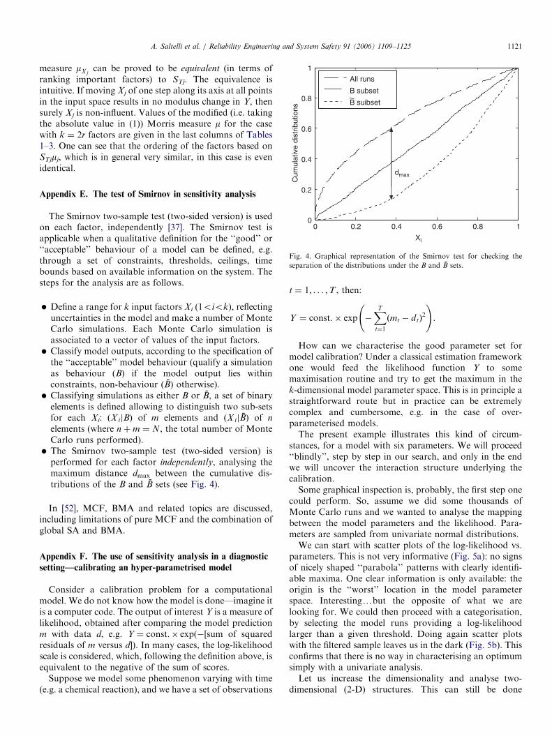
Fig. 4. Graphical representation of the Smirnov test for checking the

separation of the distributions under the B and B sets.

A. Saltelli et al. / Reliability Engineering and System Safety 91 (2006) 1109–1125 1121

measure mXjcan be proved to be equivalent (in terms of

ranking important factors) to STj. The equivalence isintuitive. If moving Xj of one step along its axis at all pointsin the input space results in no modulus change in Y, thensurely Xj is non-influent. Values of the modified (i.e. takingthe absolute value in (1)) Morris measure m for the casewith k ¼ 2r factors are given in the last columns of Tables1–3. One can see that the ordering of the factors based onSTjmj, which is in general very similar, in this case is evenidentical.

Appendix E. The test of Smirnov in sensitivity analysis

The Smirnov two-sample test (two-sided version) is usedon each factor, independently [37]. The Smirnov test isapplicable when a qualitative definition for the ‘‘good’’ or‘‘acceptable’’ behaviour of a model can be defined, e.g.through a set of constraints, thresholds, ceilings, timebounds based on available information on the system. Thesteps for the analysis are as follows.

Define a range for k input factors Xi (1oiok), reflectinguncertainties in the model and make a number of MonteCarlo simulations. Each Monte Carlo simulation isassociated to a vector of values of the input factors. Classify model outputs, according to the specification of

the ‘‘acceptable’’ model behaviour (qualify a simulationas behaviour (B) if the model output lies withinconstraints, non-behaviour (B) otherwise).

Classifying simulations as either B or B, a set of binary

elements is defined allowing to distinguish two sub-setsfor each Xi: ðX ijBÞ of m elements and ðX ijBÞ of n

elements (where nþm ¼ N, the total number of MonteCarlo runs performed).

The Smirnov two-sample test (two-sided version) is

performed for each factor independently, analysing themaximum distance dmax between the cumulative dis-tributions of the B and B sets (see Fig. 4).

In [52], MCF, BMA and related topics are discussed,including limitations of pure MCF and the combination ofglobal SA and BMA.

Appendix F. The use of sensitivity analysis in a diagnostic

setting—calibrating an hyper-parametrised model

Consider a calibration problem for a computationalmodel. We do not know how the model is done—imagine itis a computer code. The output of interest Y is a measure oflikelihood, obtained after comparing the model predictionm with data d, e.g. Y ¼ const. exp([sum of squaredresiduals of m versus d]). In many cases, the log-likelihoodscale is considered, which, following the definition above, isequivalent to the negative of the sum of scores.

Suppose we model some phenomenon varying with time(e.g. a chemical reaction), and we have a set of observations

t ¼ 1; . . . ;T , then:

Y ¼ const: exp XT

t¼1

ðmt dtÞ2

!.

How can we characterise the good parameter set formodel calibration? Under a classical estimation frameworkone would feed the likelihood function Y to somemaximisation routine and try to get the maximum in thek-dimensional model parameter space. This is in principle astraightforward route but in practice can be extremelycomplex and cumbersome, e.g. in the case of over-parameterised models.The present example illustrates this kind of circum-

stances, for a model with six parameters. We will proceed‘‘blindly’’, step by step in our search, and only in the endwe will uncover the interaction structure underlying thecalibration.Some graphical inspection is, probably, the first step one

could perform. So, assume we did some thousands ofMonte Carlo runs and we wanted to analyse the mappingbetween the model parameters and the likelihood. Para-meters are sampled from univariate normal distributions.We can start with scatter plots of the log-likelihood vs.

parameters. This is not very informative (Fig. 5a): no signsof nicely shaped ‘‘parabola’’ patterns with clearly identifi-able maxima. One clear information is only available: theorigin is the ‘‘worst’’ location in the model parameterspace. Interestingybut the opposite of what we arelooking for. We could then proceed with a categorisation,by selecting the model runs providing a log-likelihoodlarger than a given threshold. Doing again scatter plotswith the filtered sample leaves us in the dark (Fig. 5b). Thisconfirms that there is no way in characterising an optimumsimply with a univariate analysis.Let us increase the dimensionality and analyse two-

dimensional (2-D) structures. This can still be done

ARTICLE IN PRESS

-2 0 2-2000

-1500

-1000

-500

0

(a) Xi

Xi

log-

likel

ihoo

dlo

g-lik

elih

ood

-2 0 2-200

-150

-100

-50

0

(b)

Fig. 5. (a) Log-likelihood vs. a generic input factor (patterns for all input

factors are indistinguishable). (b) Same as (a) but filtering the sample for

values of log-likelihood 4200 (patterns for all input factors are

indistinguishable).

-2 0 2-2

-1

0

1

2

(a) Xi

Xi

Xj

Xj

-2 0 2-2

-1

0

1

2

(b)

Fig. 6. (a) Pairwise scatterplots of the input sample for a generic couple of

input factors (patterns for all couples are indistinguishable) (b) same as

(a), but using the filtered sample for values of log-likelihood 4200(patterns for all couples are again indistinguishable).

A. Saltelli et al. / Reliability Engineering and System Safety 91 (2006) 1109–11251122

graphically analysing 2-D projections of the Monte Carlosample onto planes defined by couples of model parameters(i.e. again under the form of scatter plots). Comparingthe 2-D projections of the original Monte Carlo sample(Fig. 6a) to those of the filtered sample (Fig. 6b) is like-wise non-informative: no difference can be noticed afterthe categorisation. Note that even if we computed on thefiltered input factors (Fig. 6b) the pairwise correlationcoefficients we would obtain zeros. Also Principal Compo-nent Analysis would not be informative as applied to thefiltered input sample, as there are no correlations amongthe filtered factors. So, it seems that there does not existany 2-D elementary structure allowing characterisingsomehow the interaction structure binding parametersunder ‘‘good’’ behaviour. We should then move to higherdimensions. Graphically? This becomes cumbersome: howto visualise scatter plots in 3-D? Correlation analysis isclearly limited to 2-D structures, so, what can we do?

SA is able to quantify the effect of model parametersunder interaction structures of any order. In this context,we extend the meaning of SA, which is not only to quantifyand rank in order of importance the sources of prediction

uncertainty, but, which is much more relevant to calibra-tion, to identify the elements (parameters, assumptions,structures, etc.) that are mostly responsible for the modelrealisations in the acceptable range.Computing the first order sensitivity indices for the log-

likelihood and the second order ones (Fig. 7), a story startsto emerge; there are non- zero second order effects, butonly within the closed groups involving factors (X1, X2, X3)and (X4, X5, X6).Computing the third order effects (Fig. 8) only

S123;S456a0. Regrouping and adding the terms up givesan interesting result:

Sc123 ¼ S1 þ S2 þ S3 þ S12 þ S13 þ S23 þ S123 ¼ 0:5,

Sc456 ¼ S4 þ S5 þ S6 þ S45 þ S46 þ S56 þ S456 ¼ 0:5,

where we have used the supescript c symbol to denote theeffects closed within the indices. The variance of theproblem is characterised by two groups of three factors.Higher term orders are zero.

ARTICLE IN PRESS

x1 x2 x3 x4 x5 x60

0.05

0.1

0.15

0.2Main effects

S12 S13 S14 S15 S16 S23 S24 S25 S26 S34 S35 S36 S45 S46 S560

0.01

0.02

0.03

0.042nd order interaction effects

[x4-x5]

[x4-x6]

[x5-x6]

[x1-x2]

[x1-x3]

[x2-x3]

Fig. 7. First and second order sensitivity indices for the log-likelihood.

S123... ...S126... S136... ...S234... ...S346 ...S4560

2

4

6

8x 10-3

Fig. 8. Third order sensitivity indices for the log-likelihood.

A. Saltelli et al. / Reliability Engineering and System Safety 91 (2006) 1109–1125 1123

This leads the investigator to conclude that what couldbe reasonably estimated are two unknown functions of twoparameter sub-sets. We can now reveal that the unknownlog-likelihood function to optimise was the sum of twospheres.

f ðX 1; . . . ;X 6Þ ¼

ffiffiffiffiffiffiffiffiffiffiffiffiffiffiffiffiffiffiffiffiffiffiffiffiffiffiffiffiffiffiX 2

1 þ X 22 þ X 2

3

q R1

2

=A1

ffiffiffiffiffiffiffiffiffiffiffiffiffiffiffiffiffiffiffiffiffiffiffiffiffiffiffiffiffiffiX 2

4 þ X 25 þ X 2

6

q R2

2

=A2.

Were the investigator to identify this structure, by trialand error, he/she would conclude that all that estimationcan provide are the two radiuses.

To this goal, the information of the ‘‘worst’’ locationcould have been useful. The easiest structure leaving outthe origin is a spherical symmetry. But in which dimen-

sions? There are as many as6

2

¼ 15 2-D;

6

3

¼ 20

3-D,6

4

¼ 15 4-D;

6

5

¼ 6 5-D spheres. May be too

many for a blind search. SA has been helpful in driving theanalysis to the correct solution!

In conclusion, where a classical estimation approach isimpractical and model factors cannot be defined, nor theclear definition of a well defined model structure or set ofhypotheses can be established, applying, e.g. standardstatistical testing procedures, SA becomes an essential tool.

ARTICLE IN PRESSA. Saltelli et al. / Reliability Engineering and System Safety 91 (2006) 1109–11251124

Model factors can be classified, e.g. as ‘‘important/unimportant’’ according to their capability of driving themodel behaviour. Such capability is clearly highlighted bythe SA, which plays a similar role, e.g. of a t-test on a least-squares estimate of a linear model. To exemplify therelevance of SA in this context, one could say that‘‘sensitivity indices are to calibration, what standardstatistical tests are to estimation’’ [52].

References

[1] Rabitz H. System analysis at molecular scale. Science 1989;246:221–6.

[2] Turanyi T, Rabitz H. Local methods and their applications. In:

Saltelli A, Chan K, Scott M, editors. Sensitivity analysis. New York:

Wiley; 2000. p. 367–83. For automated differentiation see Grievank

A. Evaluating derivatives. Principles and techniques of algorithmic

differentiation. Philadelphia, PA: SIAM; 2000.

[3] Varma A, Morbidelli M, Wu H. Parametric sensitivity in chemical

systems. Cambridge Series in Chemical Engineering, 1999.

[4] Goldsmith CH. Sensitivity analysis. In: Armitage P, Theodore C,

editors. Encyclopedia of biostatistics. New York: Wiley; 1998.

[5] Helton JC. Uncertainty and sensitivity analysis techniques for use in

performance assessment for radioactive waste disposal. Reliab Eng

Syst Saf 1993;42:327–67.

[6] Iman R L, Hora S C. A robust measure of uncertainty importance for

use in fault tree system analysis. Risk Anal 1990;10(3):401–6.

[7] Sobol’ IM. Sensitivity estimates for nonlinear mathematical models.

Mat. Model. 1990;2:112–8 (in Russian, translated in Math Model

Comput Exp 1993; 1: 407–414).

[8] Sacks J, Welch WJ, Mitchell TJ, Wynn HP. Design and analysis of

computer experiments. Stat Sci 1989;4:409–35.

[9] Campolongo F, Saltelli A, Jensen NR, Wilson J, Hjorth J. The role of

multiphase chemistry in the oxidation of dimethylsulphide (DMS). A

latitude dependent analysis. J Atmos Chem 1999;32:327–56.

[10] Campolongo F, Tarantola S, Saltelli A. Tackling quantitatively large

dimensionality problems. Comput Phys Commun 1999;117:75–85.

[11] Kioutsioukis I, Tarantola S, Saltelli A, Gatelli D. Uncertainty and

global sensitivity analysis of road transport emission estimates.

Atmos Environ 2004;38(38):6609–20.

[12] Zaldivar J-M, Campolongo F. An application of sensitivity analysis

to fish population dynamics. In: Saltelli et al., editors. Sensitivity

analysis. New York: Wiley; 2000. p. 367–83.

[13] Tarantola S, Jesinghaus J, Puolamaa M. In: Saltelli et al., editors.

Sensitivity analysis. New York: Wiley; 2000. p. 385–97.

[14] Campolongo F, Rossi A. In: Proceedings of the PSAM6, sixth

international conference on probabilistic safety assessment and

management, Puerto Rico, June 23–28, 2002. See also Chapter 6 in

Saltelli et al. Sensitivity analysis in practice. A guide to assessing

scientific models. New York: Wiley; 2004.

[15] Saltelli A. Making best use of model evaluations to compute

sensitivity indices. Comput Phys Commun 2002;145:280–97.

[16] Saltelli A, Tarantola S. On the relative importance of input factors in

mathematical models: safety assessment for nuclear waste disposal.

J Am Stat Assoc 2002;97(459):702–9.

[17] Crosetto M, Tarantola S. Uncertainty and sensitivity analysis: tools

for GIS-based model implementation. Int J Geogr Inform Sci

2001;15(4):415–37.

[18] Pastorelli R, Tarantola S, Beghi M G, Bottani C E, Saltelli A. Design

of surface Brillouin scattering experiments by sensitivity analysis.

Surf Sci 2000;468:37–50.

[19] Saltelli A, Chan K, Scott M, editors. Sensitivity analysis. New York:

Wiley; 2000.

[20] Saltelli A, Tarantola S, Campolongo F. Sensitivity analysis as an

ingredient of modelling. Stat Sci 2000;15(4):377–95.

[21] Saltelli A, Chan K, Scott M, editors. Special Issue on sensitivity

analysis. Comput Phys Commun 1999; 117 (1,2).

[22] Frey HC, Patil SR. Identification and review of sensitivity analysis

methods. Risk Anal 2002;22(3):553–78.

[23] Saisana M, Tarantola S. State-of-the-art report on current meth-

odologies and practices for composite indicator development. EUR

20408 EN, European Commission, Joint Research Centre, 2002.

[24] Saisana M, Saltelli A, Tarantola S. Uncertainty and sensitivity

analysis techniques as tools for the quality assessment of composite

indicators. J R Stat Soc A 2005;168(2):1–17.

[25] Tarantola S, Saisana M, Saltelli A, Schmiedel F, Leapman N.

Statistical Techniques and participatory approaches for the composi-

tion of the European Internal Market Index 1992-2001, EUR 20547

EN, 2002.

[26] EC, 2000, European Commission’s communication on extended

impact assessment Brussels, 05/06/2002 COM(2002) 276 final.

Guidelines for implementing the directive are available at the

Governance page of the EC http://europa.eu.int/comm/governance/

docs/index_en.htm

[27] IPCC, 2000, Good practice guidance and uncertainty management in

National Greenhouse Gas Inventories, http://www.ipcc-nggip.

iges.or.jp/public/gp/gpgaum.htm

[28] IPCC, 1999, Background papers—IPCC expert meetings on good

practice guidance and uncertainty management in National Green-

house Gas Inventories, http://www.ipcc-nggip.iges.or.jp/public/gp/

gpg-bgp.htm

[29] Frey HC. Guest Editorial. Risk Anal 2002; 22(3): 539–46.

[30] Saltelli A. Sensitivity analysis for importance assessment. Risk Anal

2002;22:579–90.

[31] Funtowicz S, Ravetz JR. Science for the post-normal age. Futures

1993;25:735–55.

[32] Funtowicz S, Ravetz JR. Post-normal science—an insight now

maturing. Futures 1999;31:641–6.

[33] Funtowicz S, Ravetz JR. A new scientific methodology for global

environmental issues. In: Costanza R, editor. Ecological economics.

New York: Columbia; 1991. p. 137–52.

[34] Funtowicz S, Ravetz JR. Three types of risk assessment and

the emergence of post-normal science. In: Krimsky S, Golding D,

editors. Social theories of risk. Westport, CT: Greenwood; 1992.

p. 251–73.

[35] Gibbons M, Limoges C, Nowotny H, Schwartzman S, Scott P, Trow

M. The new production of knowledge. The dynamics of science and

research in contemporary societies. London: Sage; 1994.

[36] Saltelli A, Funtowicz S. The precautionary principle: implications for

risk management strategies. Eur J Oncol 2003;2:67–80.

[37] Hornberger GM, Spear RC. An approach to the preliminary analysis

of environmental systems. J Env Manage 1981;12:7–18.

[38] Mac Lane S. IIASA’s credibility. Science 1988;241:1144.

[39] Mac Lane S. IIASA and modeling. Science 1988;242:1623–4.

[40] Konikov LF, Bredehoeft JD. Groundwater models cannot be

validated. Adv Water Res 1992;15(1):75–83.

[41] Oreskes N, Shrader-Frechette K, Belitz K. Verification, validation,

and confirmation of numerical models in the earth sciences. Science

1994;263:641–6.

[42] Van der Sluijs JP. A way out of the credibility crisis around model—

use in integrated environmental assessment. Futures 2002;34:

133–46.

[43] Leamer EE. Sensitivity analysis would help. In: Granger CWJ, editor.

Modelling economic series. Oxford: Clarendon Press; 1990.

[44] Lemons J, Shrader-Frechette K, Cranor C. The precautionary

principle: scientific uncertainty and type I and type II errors. Found

Sci 1997;2:207–36.

[45] Box GEP, Hunter WG, Hunter JS. Statistics for experimenters. New

York: Wiley; 1978.

[46] Welch WJ, Buck RJ, Sacks J, Wynn HP, Mitchell TJ, Morris MD.

Screening, predicting, and computer experiments. Technometrics

1992;34:15–47.

[47] O’Hagan A, Kennedy MC, Oakley JE. Uncertainty analysis and

other inference tools for complex computer codes (with discussion).

Bayesian Stat 1999;6:503–24.

ARTICLE IN PRESSA. Saltelli et al. / Reliability Engineering and System Safety 91 (2006) 1109–1125 1125

[48] Oakley J, O’Hagan A. Probabilistic sensitivity analysis of complex

models: a Bayesian approach. J R Stat Soc Ser B 2004;66:751–69.

[49] Rosen R. A comprehensive inquiry into the nature, origin, and

fabrication of life. New York: Columbia University Press; 1991.

[50] Beck MB, Ravetz JR, Mulkey LA, Barnwell TO. On the problem of

model validation for predictive exposure assessments. Stoch Hydrol

Hydraul 1997;11:229–54.

[51] Draper NR, Smith H. Applied regression analysis. New York: Wiley;

1981.

[52] Saltelli A, Tarantola S, Campolongo F, Ratto M. Sensitivity analysis

in practice. A guide to assessing scientific models. New York: Wiley;

2004.

[53] Hoeting JA, Madigan D, Rafetry AE, Volinsky CT. Bayesian model

averaging: a tutorial. Stat Sci 1999;14:382–417.

[54] Kass RE, Raftery AE. Bayes factors. J Am Stat Assoc 1995;

90(430):773–95.

[55] Saltelli A, Planas C, Tarantola S, Campolongo F. The concept of

sensitivity with applications to official statistics. Res Off Stat 1999; 2:

47–77. See also Planas and Depoutot. In: Saltelli et al., editors.

Sensitivity analysis. New York: Wiley; 2000. p. 367–83.

[56] Ratto M, Tarantola S, Saltelli A, Young PC. J R Stat Soc Ser B,

2004, submitted for publication.

[57] Morris MD. Factorial sampling plans for preliminary computational

experiments. Technometrics 1991;33(2):161–74.

[58] Spear RC, Hornberger GM. Eutrohpication in the peel inlet II:

identification of critical uncertainties via generalized sensitivity

analysis. Water Res 1980;14:43–9.

[59] Saltelli A. Sensitivity analysis. Could better methods be used?

J Geophys Res 1999;104(D3):3789–93 [plus 1999; 104(D19): 24,013].

[60] Blower SM, Gershengorn HB, Grant RM. A tale of two futures: HIV

and antiretroviral therapy in San Francisco. Science 2000;287:650–4.

[61] Valleron A-J, Boelle P-Y, Will R, Cesbron J-Y. Estimation of

epidemic size and incubation time based on age characteristics of

vCJD in the United Kingdom. Science 2001;294:1726–8 [in Reports].

[62] Halloran ME, Longini Jr IM, Nizam A, Yang Y. Containing

bioterrorist smallpox. Science 2002;298:1428–32 [in Reports].

[63] Wilmoth JR, Deegan LJ, Lundstrom H, Horiuchi S. Increase of

maximum life-span in Sweden, 1861–1999. Science 2000;289:2366–8

[in Reports].

[64] Neutel A-M, Heesterbeek JAP, De Ruiter PC. Stability in real food

webs: weak links in long loops. Science 2002;296:1120–3 [in Reports].

[65] Dundr M, Hoffmann-Rohrer U, Hu Q, Grummt I, Rothblum LI,

Phair RD, et al. A kinetic framework for a mammalian RNA

polymerase in vivo. Science 2002;298:1623–6 [in Reports].

[66] Kitano H. Systems biology: a brief overview. Science 2002;295:

1662–4 [in Review].

[67] Brookmeyer R, Blades N. Prevention of inhalational anthrax in the

US outbreak. Science 2002;295:1861 [in Brevia].

[68] Royer DL, Wing SL, Beerling DJ, Jolley DW, Koch PL, Hickey LJ,

et al. Paleobotanical evidence for near present-day levels of

atmospheric CO2 during part of the tertiary. Science 2001;292:

2310–3 [in Reports].

[69] Duarte CM, Agustı S. The CO2 balance of unproductive aquatic

ecosystems. Science 1998;281:234–6 [in Reports].

[70] Berger A, Loutre MF, McIntyre A. Intertropical latitudes and

precessional and half-precessional cycles. Science 1997;278:1476–8 [in

Technical Comments].

[71] Lipsitch M, Cohen T, Cooper B, Robins JM, Ma S, James L, et al.

Transmission dynamics and control of severe acute respiratory

syndrome. Science 2003;300:1966–70 [Published online May 23,

2003].

[72] Gu L, Baldocchi DD, Wofsy SC, Munger JW, Michalsky JJ,

Urbanski SP, et al. A response of a deciduous forest to the Mount

Pinatubo eruption: enhanced photosynthesis. Science 2003;299:

2035–8.

[73] Balmford A, Bruner A, Cooper P, Costanza R, Farber S, Green RE,

et al. Economic reasons for conserving wild nature. Science

2002;297:950–3.

[74] Medley GF. Predicting the unpredictable. Science 2001;294:1663–4.

[75] Reilly J, Stone PH, Forest CE, Webster MD, Jacoby HD, Prinn RG.

Uncertainty and climate change assessments. Science 2001;293:

430–3.

[76] Smith AE, Slepchenko BM, Schaff JC, Loew LM, Macara IG.

Systems analysis of ran transport. Science 2002;295:488–91 [in

Reports].

[77] Kao RR, Gravenor MB, Baylis M, Bostock CJ, Chihota CM, Evans

JC, et al. The potential size and duration of an epidemic of bovine

spongiform encephalopathy in British sheep. Science 2001;295:332–5

[Published online November 22, 2001].

[78] Rojstaczer S, Sterling SM, Moore NJ. Human appropriation of

photosynthesis products. Science 2001;294:2549–52 [in Reports].

[79] Sala OE, Chapin III FS, Armesto JJ, Berlow E, Bloomfield J, Dirzo

R, et al. Global biodiversity scenarios for the year 2100. Science

2000;287:1770–4 [in Review].

[80] Berner RA, Petsch ST, Lake JA, Beerling DJ, Popp BN, Lane RS,

et al. Isotope fractionation and atmospheric oxygen: implications for

phanerozoic O2 evolution. Science 2000;287:1630–3 [in Reports].

[81] Berner RA. Geochemistry and geophysics: the rise of plants and their

effect on weathering and atmospheric CO2. Science 1997;276:544–6

[in Perspectives].

[82] Gumbsch P. Materials science: enhanced: a dislocation crash test.

Science 1998;279:1489–90 [in Research].

[83] Kremen C, Niles JO, Dalton MG, Daily GC, Ehrlich PR, Fay JP,

et al. Economic incentives for rain forest conservation across scales.

Science 2000;288:1828–32.

[84] Druffel ERM. Pulses of rapid ventilation in the North Atlantic

surface ocean during the past century. Science 1997;275:

1454–7.

[85] Eisenmesser EZ, Bosco DA, Akke M, Kern D. Enzyme dynamics

during catalysis. Science 2002;295:1520–3 [in Reports].

[86] Jamison DT, Sandbu ME. Global health: who ranking of health

system performance. Science 2001;293:1595–6 [in Policy Forum].

[87] Jolly D, Haxeltine A. Effect of low glacial atmospheric CO2 on

tropical African Montane vegetation. Science 1997;276:786–8 [in

Reports].

[88] Lewison JGG, May RM. Government funding of research and

development. Science 1997;278:878–80 [in Technical Comments].

[89] Moolgavkar SH. Consideration of copollutants. Science 2000;

290:453.

[90] Apted MJ, Langmuir D, Moeller DW, Ahn J, Waltar AE, von

Winterfeldt D, et al. Yucca Mountain: should we delay? Science

2002;296:2333–5.

[91] Chesler EJ, Rodriguez-Zas SL, Mogil JS, Darvasi A, Usuka J, Grupe

A, et al. In silico mapping of mouse quantitative trait loci. Science

2001;294:2423 [in Technical Comments].

[92] Davenport MP, Blower SM, Gershengorn HB, Grant RM. Rever-

sibility of HIV drug resistance. Science 2000;288:1299.

[93] Campolongo F, Cariboni J, Saltelli A. 2004, in preparation.