Reviews - University of Colorado Boulder

Journal of the Indian Institute of Science

A Multidisciplinary Reviews Journal

ISSN: 0970-4140 Coden-JIISAD

© Indian Institute of Science

Journal of the Indian Institute of Science VOL 93:3 Jul.–Sep. 2013 journal.iisc.ernet.in

Rev

iew

s

Department of Computer Science and EngineeringIndian Institute of Technology BombayMumbai, India 400076

[email protected]

[email protected]

Hybrid Automata for Formal Modeling and Verification of Cyber-Physical Systems

Shankara Narayanan Krishna and Ashutosh Trivedi

Abstract | The presence of a tight integration between the discrete control (the “cyber”) and the analog environment (the “physical”)—via sensors and actuators over wired or wireless communication networks—is the defining feature of cyber-physical systems. Hence, the functional correctness of a cyber-physical system is crucially dependent not only on the dynamics of the analog physical environment, but also on the decisions taken by the discrete control that alter the dynamics of the environment. The framework of Hybrid automata—introduced by Alur, Courcoubetis, Henzinger, and Ho—provides a formal modeling and specification environment to analyze the interaction between the discrete and the continuous parts of cyber-physical systems. Hybrid automata can be considered as generalizations of finite state automata augmented with a finite set of real-valued variables whose dynamics in each state is governed by a system of ordinary dif-ferential equations. Moreover, the discrete transitions of hybrid automata are guarded by constraints over the values of these real-valued variables, and enable discontinuous jumps in the evolution of these variables. Con-sidering the richness of the dynamics in a hybrid automaton, it is perhaps not surprising that the fundamental verification questions, like reachabil-ity and schedulability, for the general model are undecidable. In this arti-cle we present a review of hybrid automata as modeling and verification framework for cyber-physical systems, and survey some of the key results related to practical verification questions related to hybrid automata.Keywords: Cyber-Physical Systems, Dynamical Systems, Formal Modeling, Formal Verification, LTL Model-Checking, Timed Automata, Hybrid Automata.

1 IntroductionThe term “cyber-physical systems” refers to any network of digital and analog systems whose per-formance crucially depends on both the continu-ous dynamics of the analog parts and the real-time switching decisions made by the digital system. A typical cyber-physical system may consist of several processors connected with a set of physical systems via sensors and actuators over wired or wireless com-munication networks. Such systems are increasingly playing safety-critical role in modern life, where a fault in their design can be catastrophic.

Modern cars are an important paradigmatic example of such safety-critical cyber-physical

systems. A modern premium car typically has 70 to 100 interconnected electronic control units (ECUs) with dozens of sensors39 performing various func-tions44 like air-bag control, cruise control, electronic stability control, antilock brakes, engine ignition, windshield-wiper control, engine control, and collision-avoidance system. Many of these ECUs are connected with analog environment via sensors and actuators, and are expected to perform their operations within hard time limits. For instance, the air-bag ECU needs to respond within 20–30 mil-lisecond after the impact sensor connected to it detects a severe impact. As the number of ECUs in a typical car is increasing and performing more


Journal of the Indian Institute of Science VOL 93:3 Jul.–Sep. 2013 journal.iisc.ernet.in420

autonomously, it is becoming increasingly difficult to ensure their correctness. The severity of the prob-lem can perhaps be best realized by looking into the growing list of recalls44 by leading car companies due to software-related problems. Some promi-nent examples include Toyota’s recall of 160,000 of its 2004/05 Prius models because of a software problem causing the car to suddenly stall, Jaguar’s 2011 recall of nearly 18,000 X-type cars due to a software bug resulting in driver’s inability in turn-ing off the cruise control, and Volkswagen’s 2011 recall of about 4000 of its 2008 Passats models for engine-control module software problem. The list is long and underscores the challenges in designing and verifying safety-critical cyber-physical systems. Similar examples can also be cited for the cyber-physical system from other domains such as avion-ics, implantable medical devices, transportation networks, and energy sector.

Formal modeling and verification of systems is the set of techniques that employ rigorous math-ematical reasoning to analyze properties of a system. In this article we concentrate on a celebrated3,4 formal verification framework known as model checking.50 Model Checking—pioneered by Clarke, Sifakis and Emerson2—is a widely used automated technique that, given a formal description of a system and a property, systematically checks whether this prop-erty holds for a given state of the system model. The three key steps of this framework are the following:

1. formal modeling: modeling a system under consideration using mathematically precise syntax that approximate a given system to a desired level of abstraction;

2. formal specification: specify the properties of the system using some mathematically precise speci-fication language (typically in formal logic); and

3. formal analysis: analyze the formal model with respect to the formal specification and report counter-example in case the system model vio-lates the specification.

The success of the model checking framework in formal verification of systems is largely due to it being highly automatic—a push-button technology47—in comparison to other competing approaches like theorem proving. The counterexamples generated in the model-checking process often are used to auto-matically refine—known as counterexample-guided abstraction refinement (CEGAR)48,49 framework—the model and/or the property and the entire proce-dure can be repeated and thus removing the need of a very accurate initial model or specification.

Early research on formal modeling and verifica-tion of systems concentrated on simplified models

of the systems as finite state-transition graphs. Since these models are finite in nature, it is—in theory—possible to exhaustively explore the state space of the system to verify the properties of interest. How-ever, the biggest challenge in model-checking of finite state-transition graphs is so-called state-space explosion problem50 characterizing the exponential blowup in the number of states in the explicit rep-resentation of the system where the system is natu-rally represented succinctly using state variables, or as a composition of a network of interacting finite state-transition graphs. In general, the state-space explosion problem renders the explicit exhaustive exploration of the system intractable. However, a number of techniques have been proposed to over-come the state-space explosion problem—including symmetry reduction,46 partial-order reduction,85 symbolic model checking80 and bounded model checking29,30—that has culminated into efficient and mature tool support including SPIN92 and NuSMV82 for finite state model-checking. Examples of the use of finite-state model-checking in indus-try include the verification of hardware circuits,67 communication15 and security24,78 protocols, and software device drivers.23

These finite state-transition graphs, however, often do not satisfactorily model cyber-physical systems as they disregard the continuous dynamics of the physical environment. Alur and Dill10 were the first one to propose a formal model, known as timed automata, combining finite state-transition graphs with a finite set of real-valued variables that evolve as time progresses while the system occupies a state. In a timed automaton the real-valued variables—called clocks—simulate per-fect clocks as they evolve with a uniform constant speed (rate) and hence can model asynchronous real-time systems interacting with a continuous physical environment. The clock variables can be used to constrain the evolution of the system by guarding the transitions of the graph, and can also be reset at the time of taking a transition to remember the time since that transition. These capabilities make timed automata quite expressive formalism to define real-time systems. Moreover, the decidabilitya of key verification problems like

a The concept of decidability is a central one in computer sci-

ence and it characterizes the set of problems for which one can

write computer programs that always terminate with a correct

answer. The problems for which it is not possible to write such

a program are known as undecidable problems. A most famous

undecidable problem is the halting problem (similar to reach-

ability problem) for the configurations of Turing machines (an

abstract model of computation capturing the notion of algo-

rithmic computation).


Journal of the Indian Institute of Science VOL 93:3 Jul.–Sep. 2013 journal.iisc.ernet.in 421

reachability and schedulability10 and availability of mature verification tools—like UPPAAL,27,96 Kronos,66 and RED89—make timed automata an appealing tool for real-time system verification.

Alur, Courcoubetis, Henzinger, and Ho gen-eralized the timed automata to hybrid automata9 to include real-valued variables with arbitrary dynamics specified using ordinary differential equations. Considering the richness of dynamics of a hybrid automata, it is perhaps not surprising that the fundamental verification questions like reachability are undecidable for hybrid autom-ata. A number of subclasses of hybrid automata has been proposed with decidable verification problems and some of the algorithms have been implemented as part of tools like HyTech60 and PHAVer.86

Timed and hybrid automata provide an intui-tive and semantically unambiguous way to model cyber-physical systems, and a number of case-studies41,55,61,74,84,93,95 demonstrate their application for the analysis of cyber-physical systems. In this article we aim to provide a general introduction to verification using hybrid automata as we focus on model-checking classical LTL logic77 over hybrid automata. To keep the discussion simple we do not cover other logics, for instance, computation tree logic (CTL, CTL*),50,77 modal µ-calculus,53 and real-time and hybrid extensions of these logics14 including metric temporal logics (MTL)65,83 and duration calculus (DC).43

The goal of this article is to introduce key con-cepts for cyber-physical system modeling and verification using hybrid automata with a focus on LTL model-checking. In order to better focus our attention, we will not cover several useful extensions of hybrid automata that capture cer-tain natural aspects of modeling hybrid systems, including

– game-theoretic extensions7,17,20,32,45,52 that allow the model to distinguish between controllable and uncontrollable non-determinism;

– probabilistic extensions6,25,36,68,71,75 that permit modeling of stochastic behavior arising due to, e.g., faulty or unreliable sensors or actuators, uncertainty in timing delays, and performance characteristics of (third-party) components; and

– priced extensions28,31,33,73,88 that permit mod-eling of resource consumption and payoffs associated with decisions.

We also restrict our attention to theoreti-cal results regarding decidability of LTL model- checking problems, and do not cover data

structures and algorithms27,54,57 for efficient imple-mentation of these results.

We begin (Section 2) this survey by intro-ducing two formalisms to model discrete and continuous dynamical systems, and then we present hybrid automata model that combines features from these two models. Section 3 intro-duces syntax and semantics of linear temporal logic (LTL) followed by a formal definition of corresponding model-checking problem over a hybrid automata, and using two-counter Minsky machines81 we prove the in general LTL model-checking over hybrid automata is undecidable. In this section, we also introduce the idea of state-space reduction using a well-established technique called quotienting which we later exploit to show decidability of model checking problem for some variants of hybrid automata. We conclude the survey by discussing (Section 4) three key subclasses of hybrid automata—timed automata, (initialized) rectangular hybrid automata, and (two dimensional) piecewise-constant derivative systems—with decidable model checking problem.

2 Hybrid AutomataA dynamical system is simply a system whose “state” evolves with “time” governed by a fixed set of rules or “dynamics”. The state of a dynami-cal system is specified as valuations of the vari-ables of interest in the system. Depending upon the nature of variables (discrete or continuous) and the notion of time (discrete or continu-ous) the dynamics of variables can be specified by differential equations or discrete assign-ments. For the purpose of this paper, we clas-sify the dynamical systems into the following three broad classes: i) discrete systems where both the notion of time and the variables are discrete, ii) continuous systems where the notion of time is continuous, while the variables are continuous, and iii) hybrid systems where some variables are continuous and some are discrete, and although the notion of time is continuous, special dynamic-changing events can happen at discrete instants. Notice that both discrete and continuous systems can be considered as sub-classes of hybrid systems.

On an abstract level any dynamical system can simply be represented as a graph whose nodes represent the states and edges represent transition between the states. Formally, a state transition graph can be defined in the following manner.

Definition 1 (State Transition Graphs): A state transition graph is a tuple T = (S, S

0, ∑, ∆) where:



begin this section by introducing concepts and notation used throughout this article, followed by discussing such syntactical models to represent purely discrete and purely continuous dynamical system. After introducing these models we present hybrid automata capable of modeling hybrid dynamical systems.

Variables and predicatesLet R be the set of real numbers, R≥0

be the set of non-negative real numbers, and Z be the set of integers.

Let X be a set of real-valued variables. A valua-tion on X is a function v : X→R and we write V(X) for the set of valuations on X. Abusing notation, we also treat a valuation v as a point in Rn that is equipped with the standard Euclidean norm ||⋅|| where n is the cardinality of X.

We define a predicate over a set X as a subset of R|X|. For efficient computer-readable represen-tation of predicates we often define them using non-linear algebraic equations involving X. We write pred(X) for the set of predicates over X. For a predicate π ∈ pred(X) we write π for the set of valuations in R|X| satisfying the equation π. We write for the predicate that is true for all valu-ations, while for the predicate which is false for all the valuations.

Example 2: An example of a predicate over the variables θ and θ is

m mg θ θ= − ,sin( )

characterizing the motion of an idealized pendu-lum (Figure 3) where θ is the angle the pendulum forms with its rest position, θ is second deriva-tive of θ, m is the mass of the pendulum, g is the gravitational constant, and is the length of the pendulum.

We say that a predicate P is polyhedral if it is defined as a conjunction of a finite set of linear constraints of the form a

1x

1 + … + a

nx

n k, where

k ∈ Z, for all 1 ≤ i ≤ n we have that ai ∈ R, x

i ∈X,

and ∈{<, ≤, =, >, ≥}. An example of a polyhedral predicate over the set {x, y, z} is 2x + 3y – 9z ≤ 5. We define an octagonal predicate as the conjunc-tion of a finite set of linear constraints over X of the form ±x ±y k or x k, where k ∈ R, x, y ∈ X. Similarly a rectangular predicate is defined as the conjunction of a finite set of linear constraints over X of the form x k, where k ∈ R, and x ∈ X.

2.1 Discrete dynamical systemsDiscrete dynamical systems can be conveniently modeled as extended finite state machines having finitely many modes and transitions between these

Figure 1: State transition graph for a mod-4 counter.

– S is a (potentially infinite) set of states;– S

0 ⊆ S is the set of initial states;

– ∑ is a (potentially infinite) set of actions; and– ∆ ⊆ S × ∑ × S is the transition relation.

We say that a state transition graph T is finite (countable), if the sets S and ∑ are finite (countable).

Given an action a ∈ ∑ and a state s we write Post (s, a) for the set of states that are reachable from s on a and Post (s) for the states reachable in one step from s, i.e.

= ′ : , , ′ ∈∆= , .

∈

{ ( ) }( )

s s a ss a

a Σ∪

A run—an execution or a trajectory—of a dynam-ical system modeled as a state transition graph T is a (finite or infinite) alternating sequence of states and actions that begins with an initial state and all consecutive states are connected with their predecessor via the transition relation. Formally, a finite run is a sequence ⟨s

0, a

1, s

1, a

2, s

2, …, s

n⟩

such that s0 ∈ S

0 and for all 0 ≤ i < n we have that

si+1

∈ Post (si, a

i+1). An infinite run is defined

analogously.Example 1: A graphical description of a state

transition graph depicting a mod-4 counter with pause is shown in Figure 1. We represent a state using a rounded rectangle and a transition using a labeled edge between participating states. An ini-tial state is marked using an incoming arrow to that state labeled “start”. An example of a run is the finite sequence:

( ) ( ) ( )( )

count tick count pause pause tick,pause on

, , , , , , , ,, ,

0 1 11 ,, , , , , .( ) ( )count tick count1 2

A state transition graph is a feasible way to represent and computationally analyze dynami-cal systems with finitely many states. However, to enable computational analysis of a general infinite state dynamical system we need a finitary way to represent a potentially infinite space of states. We

Post(s, a) Post(s) Post



modes. The values of variables remain unchanged while the system is in some mode, and changes only when a transition takes place where they can “jump” to new values assigned by the transi-tion. These jumps are specified using predicates over the set X ∪ X′ that relates the current values of variables of system, given as the set X, to the values in the next time-step, given as the set X′ of primed-versions of variables in X. Transitions are often guarded by predicates over variables speci-fying the enabledness condition of the transition. Starting from some initial valuation to the vari-ables, a system modeled using an extended finite state machine evolves in discrete time-steps. At each discrete step the system can take any enabled transition, i.e. satisfied by the current variable valuation, and after executing the transition the valuation of the variables is changed according to the jump condition. The system continues evolv-ing in this fashion forever. An extended finite state machine is formally defined as the following.

Definition 2 (Extended Finite State Machines: Syntax): An extended finite state machine is a tuple M = (M, M

0, ∑, X, ∆, I, V

0) such that:

– M is a finite set of control modes including a distinguished initial set of control modes M

0 ⊆ M,

– ∑ is a finite set of actions,– X is a finite set of real-valued variable,– ∆ ⊆ M × pred(X) × ∑ × pred(X ∪ X′) × M is

the transition relation,– I : M → pred(X) is the mode-invariant func-

tion, and– V

0 ∈ pred(X) is the set of initial valuations.

For a transition δ = (m, g, a, j, m′) ∈ ∆ we refer to m ∈ M as its source mode, g ∈ pred(X) as its guard, a ∈ A as its action, j ∈ pred(X ∪ X′) as its jump constraint, and m′ ∈ M as the target mode.

A configuration of an extended finite state machine is a tuple (m, v) where m is a control mode and v is a valuation of variables in X. The execution of an extended finite state machine begins in a configuration (m

0, v

0) such that the

control mode m0 ∈ M

0 is in the set of initial con-

trol modes and the valuation v0 ∈ V

0 satisfies the

invariant of mode m0, i.e. v

0 ∈ I(m

0). At each

discrete time-step the system executes a transition (m, g, a, j, m′) that is enabled in the current con-figuration (m, v), i.e., v ∈ g, and the configura-tion of the system jumps to a new configuration (m′, v′) while respecting the jump constraints, i.e. (v, v′) ∈ j as well as the invariant condition of the resulting mode v′ ∈ I(m′). The system contin-ues its execution from the resulting configuration

in the similar fashion. Hence, we can define the semantics of an extended finite state machine as a state transition graph in the following manner.

Definition 3 (Extended Finite State Machine: Semantics): The semantics of an extended finite state machine M = (M, M

0, ∑, X, ∆, I, V

0) is given as

a state transition graph T S SM M M M M= ∆( , , , )0 Σ where:

– SM ⊆ (M × R|X|) is the set of configurations of M such that for all (m, v) ∈SM we have that v ∈ I(m);

– S S0M M⊆ such that (m, v) ∈ SM if m ∈ M

0

and v ∈ V0;

– ∑M = ∑ is the set of labels;– ∆M ⊆ SM × ∑M × SM is the set of transitions

such that ((m, v), a, (m′, v′)) ∈ ∆M if there exists a transition δ = (m, g, a, j, m′) ∈ ∆ such that the current valuation v satisfies the guard of δ, i.e. v ∈ g; the pair of current and next valuations (v, v′) satisfies the jump constraint of δ, i.e. (v, v′) ∈ j; and the next valuation satisfies the invariant of the target mode of δ, i.e. v′ ∈ I(m′).

Let us consider an example of the syntax and semantics of an extended finite state machine.

Example 3 (Modulo-4 counter): Let us consider a modulo-4 counter with reset and pause function-ality shown in Figure 2. This extended finite state machine M = (M, M

0, ∑, X, ∆, I, V

0) has two con-

trol modes M = {count, pause} with count being the initial mode. The variable x is the only variable, while the set of action is ∑ = {tick, on, pause} where tick, on, and pause stand for clock-tick, start-counting, and pause-counting actions, respectively. While drawing an extended finite state machine, we depict modes by rounded rectangles and transi-tions by arrows connecting the modes labeled by a triplet (g, a, j) showing the guard, the action, and the jump predicate of the transition. For example the transition (count, x = 3, tick, x′ = 0, count) is shown in the Figure 2 as a self-loop labeled with (x = 3, tick, x′ = 0) on the mode labeled count. It is straightforward to see that the extended finite state machine in Figure 2 models a modulo-4 counter

Figure 2: An EFSM description of a mod-4 counter with reset and pause.



with reset and pause. The corresponding state tran-sition graph is shown in the Figure 1.

In the rest of the article, to minimize clutter, we will omit the guard if it is the predicate , and we omit the jump predicates specifying that the value of a variable remains unchanged, i.e. predi-cates of the form x′ = x.

2.2 Continuous dynamical systemsFor the purpose of this article, a continuous dynamical system is a finite set of continuous variables along with a set of ordinary differential equations characterizing the dynamics or the flow of these variables as a function of time. We rep-resent the flow of a continuous dynamical system using a flow function F : R|X| → R|X| characterizing the system of ordinary differential equations:

X F X= ( ) (1)

where, following Newton’s dot notation for dif-ferentiation, X represents the set of first-order derivatives of the variables in the set X. Informa-tion about the higher-order derivatives can be represented using only first-order derivatives intro-ducing auxiliary variables. For example the second-order differential equation θ θ+ / =( ) sin( )g 0 can be written as a system of first-order differen-tial equations θ θ= , = − /y y g( ) sin( ) . Formally, a continuous dynamical system is defined in the following manner.

Definition 4 (Continuous Dynamical System): A continuous dynamical system is a tuple M = (X, F, v

0) such that

– X is a finite set of real-valued variable,– F : R|X| → R|X| is the flow function characteriz-

ing the the set of ordinary differential equation X F X= ( ), and

– v0 ∈ R|X| is the initial valuation.

A run of a continuous dynamical system M = (X, F, v

0) is given as a solution to the system of dif-

ferential equations (1) with initial valuation v0. Let

a differentiable function f : R≥0 →R|X| be a solution

to (1), that provides the valuations of the variables as a function of time, such that:

f v

f t F f t t

( )

( ) ( ( )) ,

0

forevery

0=

= ∈ ≥0

where f : R≥0 → R|X| is the time derivative of the

function f. We call such a function f a run of the continuous dynamical system M. Since, in gen-eral, a solution of (1) may not exist or may not be unique, a run of a continuous dynamical sys-tem may not exist or may not be unique.74 To

ensure the existence and the uniqueness of the run we enforce Lipschitz-continuityb assumption on F. The following result states the existence and uniqueness of the set of ordinary differential equa-tions (1) under Lipschitz-continuity assumption.

Theorem 1 (Picard-Lindelöf Theorem):90 If a function F: R|X| → R|X| is Lipschitz-continuous then the differential equation X F X= ( ) with ini-tial valuation v

0 ∈ R|X| has a unique solution f : R≥0

→ R|X| for all v

0 ∈ R|X|.

In addition, Lipschitz-continuity offers the following advantage while numerically simulat-ing an approximate solution to the differential equations (1).

Theorem 2 (Stability wrt initial valuation):74 Let F be a Lipschitz-continuous function with constant K > 0 and let f : R≥0

→ R|X| and f ′: R≥0

→ R|X| be solutions to the differential equation X F X= ( ) with initial valuation v

0 ∈ R|X| and ν

0′

∈R | |X , respectively. Then, for all t ∈ R≥0 we have

that ||f(t) – f ′(t)||≤||v–v0||eKt.

This theorem implies that, under Lipschitz-continuous assumption on the flow function F, any two runs whose initial valuations are close to one-another remain close as the time progresses. Since it is not always possible to analytically solve differential equations, this property permits us to numerically simulate the behaviour of continuous dynamical system using approximation methods, e.g. Euler’s method or Runge-Kutta method, that are readily available in tools such as Matlab79 and Mathematica.98

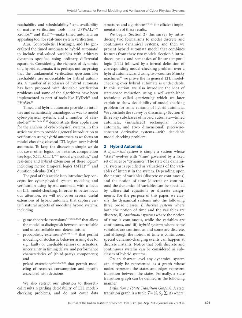
Example 4 (Simple Pendulum): Consider a simple pendulum shown in Figure 3 and its the motion equations:

θ

θ= ,= − / ,

yy g( ) sin( )

with initial valuations (θ, y) = (θ0, 0). To analyti-

cally solve these equations let us assume small enough angular displacement θ and sin(θ) ≈ θ. Now the equations simplify to

θ θ= = − / .y y gand ( )

Hence our continuous dynamical system is M = (X, F, v

0) where X = {θ, y}, F is such that F y( )θ =

and F y g( ) ( ) = − / θ and v0 = (θ

0, 0). The solution

for these differential equations is

θ( ) cos( ) sin( )( ) sin( ) cos( )t A Kt B Kt

y t AK Kt BK Kt= += − + ,

b We say that a function F : Rn → Rn is Lipschitz-continuous if

there exists a constant K > 0, called the Lipschitz constant, such

that for all x, y ∈ Rn we have that ||F(x) – F(y)|| < K ||x–y||.



where K g= /. Substituting θ(0) = θ0 and y(0) =

0 from the initial valuation, we get that A = θ0 and

B = 0. Hence the unique run of the pendulum sys-tem can be given as the function f : R≥0

→ {θ, y} as t Kt K Kt ( cos( ) sin( ))θ θ0 0,− . Figure 4 shows the change in valuations of the variables θ and y as a function of time.

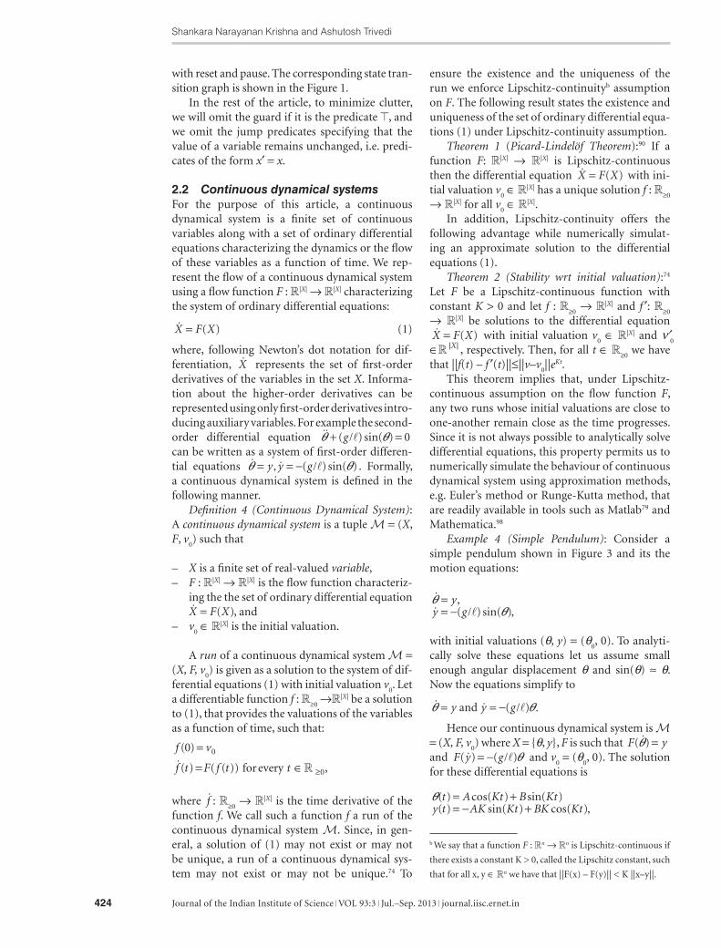
2.3 Hybrid dynamical systemsIn the previous two subsections we discussed mode-ling of purely discrete and purely continuous dynam-ical systems. We saw that in a discrete dynamical system the state of the system changes during a dis-crete transition where it “jumps” (see Figure 5) to the new value governed by the transition relation, while in a continuous system the state of the system continuously “flows” (see Figure 5) in a fashion gov-erned by ordinary differential equations. Hybrid sys-tems share their properties with both discrete as well as continuous systems, as their state progresses with

time in both discrete jumps as well as continuous flows. In this section we present hybrid automata, a combination of extended finite state machines and continuous dynamical systems, where in every control mode the dynamics of the variables of the system can be specified using ordinary differential equations.

Definition 5 (Hybrid Automata: Syntax): A hybrid automaton is a tuple H = (M, M

0, ∑, X, ∆,

I, F, V0) where:

– M is a finite set of control modes including a distinguished initial set of control modes M

0 ⊆ M,

– ∑ is a finite set of actions,– X is a finite set of real-valued variables,– ∆ ⊆ M × pred(X) × ∑ × pred(X ∪ X′) × M is

the transition relation,– I : M → pred(X) is the mode-invariant function,– F : M → (R|X| → R|X|) is the mode-dependent

flow function characterizing the flow for each mode m ∈ M as the set of ODEs X F m X= ( )( ), and

– V0 ∈ pred(X) is the set of initial valuations.

To ensure existence of unique solutions of the ODEs in flow functions, we assume that for each mode m ∈ M the flow function F(m) is Lipschitz-continuous.

Just like in an extended finite state machine, a configuration of a hybrid automaton is a tuple (m, v) where m ∈ M is a mode and v ∈ R|X| is a var-iable valuation. For a Lipschitz-continuous flow function F : M → (R|X| → R|X|), a valuation v ∈ R|X|, a mode m ∈ M, and a time delay t ∈ R≥0

we define (v⊕

F(m) t) for the unique valuation f(t) where f is

the unique run of the continuous dynamical sys-tem (X, F(m), v). For a jump predicate j ∈ pred(X ∪ X′) and valuation v we define v[j] for the set of valuations ν′ ∈R ≥0

| |X such that (v, v′) ∈ j.The execution of a hybrid automaton begins in

an initial configuration (m0, v

0) where m

0 ∈ M

0 is an

initial mode and v0 ∈ V

0 is an initial valuation sat-

isfying v0 ∈I(m

0). The system stays in a mode for

some time, say t1 ∈ R≥0

, and while the system stays in a control mode m the valuation of the variables changes according to ODE specified by the flow F(m) of the corresponding mode. After spending t

1 ∈ R≥0

time in mode m0 an enabled transition

(m0, g, a, j, m

1) is non-deterministically chosen

and executed. Notice that we say that a transition (m

0, g, a, j, m

1) is enabled if ( )( )ν0 10

⊕F m t g∈ and all the intermediate valuations that system passes through from v

0 to ( )( )ν0 10

⊕F m t satisfy the invariant of the mode m

0, i.e. for all t ∈ [0, t

1] we

have that ( ) ( )( )ν0 00⊕F m t I m∈ . After executing

Figure 3: An idealized pendulum with length l and mass m.

Figure 4: The variables θ (angle displacement) and y (angular velocity) are plotted with respect to the time for a pendulum with l = 1 meter with θ0 = 5 degrees.



the transition (m0, g, a, j, m

1) the state of the sys-

tem jumps to a new configuration (m1, v

1) such

that v1 ∈ I(m

1) and v

1 ∈ ( )[ ]( )ν0 10

⊕F m t j . The system continues its operation in a similar man-ner from the resulting configuration (m

1, v

1). We

can formalize this semantics using a (uncountably infinite) state transition graph.

Definition 6 (Hybrid Automata: Semantics): The semantics of a hybrid automaton H = (M, M

0,

∑, X, ∆, I, F, V0) is given as a state transition graph

T S SH H H H H= ∆( , , , )0 Σ where:

– SH ⊆ (M × R|X|) is the set of configurations of H such that for all (m, v) ∈ SH we have that v ∈ I(m);

– S S0H H⊆ s.t. (m, v) ∈ S0

H if m ∈ M 0 and v ∈ V

0;

– ∑H = R≥0 × ∑ is the set of labels;

– ∆H ⊆ SH × ∑H × SH is the set of transitions such that ((m, v), (t, a), (m′, v′)) ∈ ∆H if there exists a transition δ = (m, g, a, j, m′) ∈ ∆ such that– (v⊕

F(m)t) ∈ g;

– (v⊕F(m)

t) ∈ I(m) for all t ∈ [0, t];– ν ′ ∈ (ν ⊕

F(m)t)[j]; and

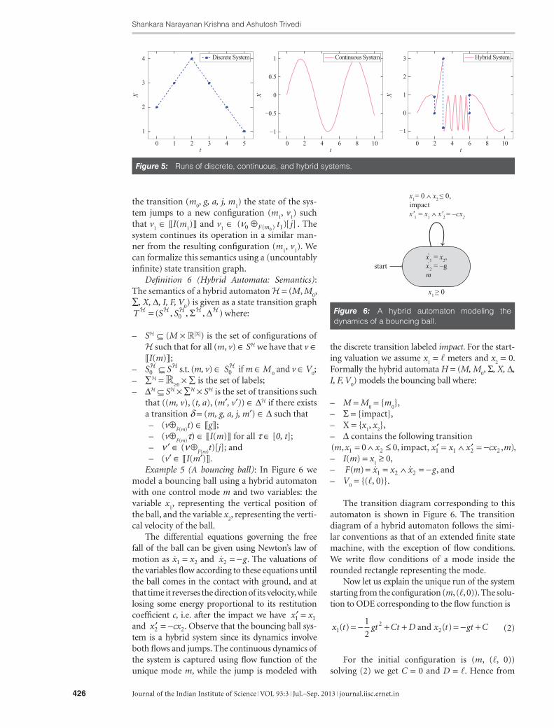
– (v′ ∈ I(m′).Example 5 (A bouncing ball): In Figure 6 we

model a bouncing ball using a hybrid automaton with one control mode m and two variables: the variable x

1, representing the vertical position of

the ball, and the variable x2, representing the verti-

cal velocity of the ball.The differential equations governing the free

fall of the ball can be given using Newton’s law of motion as x x1 2= and x g2 = − . The valuations of the variables flow according to these equations until the ball comes in the contact with ground, and at that time it reverses the direction of its velocity, while losing some energy proportional to its restitution coefficient c, i.e. after the impact we have ′ =x x1 1 and ′ = −x cx2 2. Observe that the bouncing ball sys-tem is a hybrid system since its dynamics involve both flows and jumps. The continuous dynamics of the system is captured using flow function of the unique mode m, while the jump is modeled with

the discrete transition labeled impact. For the start-ing valuation we assume x

1 = meters and x

2 = 0.

Formally the hybrid automata H = (M, M0, Σ, X, ∆,

I, F, V0) models the bouncing ball where:

– M = M0 = {m

0},

– Σ = {impact},– X = {x

1, x

2},

– ∆ contains the following transition ( )m x x x x x cx m, = ∧ ≤ , , ′ = ∧ ′ = − , ,1 2 1 1 2 20 0 impact– I(m) = x

1 ≥ 0,

– F m x x x g( ) = = ∧ = − 1 2 2 , and– V

0 = {(, 0)}.

The transition diagram corresponding to this automaton is shown in Figure 6. The transition diagram of a hybrid automaton follows the simi-lar conventions as that of an extended finite state machine, with the exception of flow conditions. We write flow conditions of a mode inside the rounded rectangle representing the mode.

Now let us explain the unique run of the system starting from the configuration (m, (, 0)). The solu-tion to ODE corresponding to the flow function is

x t gt Ct D x t gt C12

21

2( ) ( )= − + + = − +and (2)

For the initial configuration is (m, (, 0)) solving (2) we get C = 0 and D = . Hence from

Figure 6: A hybrid automaton modeling the dynamics of a bouncing ball.

Figure 5: Runs of discrete, continuous, and hybrid systems.



(m, (, 0)) system flows according to the equations x t gt1

12

2( ) = − + and x2(t) = −gt. According to

these equations the value of variable x1 continue

to fall for the next t g1 2= / time units when x

1 becomes 0, and the transition impact becomes

available and must be taken (since the invariant of the mode requires x

1 to be non-negative). Imme-

diately before taking the transition the configura-tion is (0, −gt

1). Using our notations we can write

it as (0, −gt1) = (, 0)⊕

F(m)t

1.

After taking the transition impact this valu-ation changes according to the jump function

′ = ∧ ′ = −x x x cx1 1 2 2 resulting in the new valua-tion (0, cgt

1). Again, in our notation we write

( ) ( )[ ]0 01 1 1 1 2 2, ∈ ,− ′ = ∧ ′ = −cgt gt x x x cx . The run of the system, so far, can be written as ⟨(m, (, 0)), (t

1, impact), (m, (0, cgt

1))⟩. Now from the

configuration (m, (0, cgt1)) the system can flow

continuously according to F(m). Solving (2) for this initial valuation we get C = cgt

1 and

D = 0. Hence from (m, (0, cgt1)) the system flows

according to the equations x t gt cgt t112

21( ) = − +

and x2(t) = −gt + cgt

1 for the next t

2 = 2ct

1 time

units till it reaches the valuation x1 = 0 (the ball

hits the ground again). At this point the result-ing configuration will be (0, −cgt

1) and after the

transition the configuration will be (0, c2gt1).

The system continues in this fashion forever and realizes the following infinite run of the system:

⟨( ( )) ( ) ( ( ))( ) ( (

m t m cgtct m c

, , , , , , , ,, , , ,

0 02 01 1

12

impactimpact ggt

c t m c gt1

21

312 0

))( ) ( ( )) ...

,, , , , ,impact ⟩,

(3)

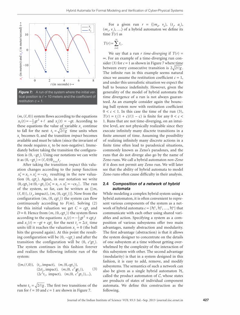
where t g1 2= / . The first two transitions of the run for = 10 and c = 1 are shown in Figure 7.

For a given run r = ⟨(m0, v

0), (t

1, a

1),

(m1, v

1), …⟩ of a hybrid automaton we define its

time T(r) as

T r ti

i( ) = .=

∞

∑1

We say that a run r time-diverging if T(r) = ∞. For an example of a time-diverging run con-sider (3) for c = 1 as shown in Figure 7 where time between every consecutive transition is 2 2/g . The infinite run in this example seems natural since we assume the restitution coefficient c = 1, and under this unrealistic situation we expect the ball to bounce indefinitely. However, given the generality of the model of hybrid automata the time divergence of a run is not always guaran-teed. As an example consider again the bounc-ing ball system now with restitution coefficient 0 < c < 1. In this case the time of the run (3), T(r) = t

1(1 + c)/(1 – c) is finite for any 0 < c <

1. Runs that are not time-diverging, on an intui-tive level, are not physically realizable since they execute infinitely many discrete transitions in a finite amount of time. Assuming the possibility of realizing infinitely many discrete actions in a finite time often lead to paradoxical situations, commonly known as Zeno’s paradoxes, and the runs that do not diverge also go by the name of Zeno runs. We call a hybrid automaton non-Zeno if it does not permit any Zeno run. We will later see that the ability of hybrid automata to model Zeno runs often cause difficulty in their analysis.

2.4 Composition of a network of hybrid automata

While modeling a complex hybrid system using a hybrid automaton, it is often convenient to repre-sent various components of the system as a net-work of hybrid automata c = {H1, H2, …, Hn} that communicate with each other using shared vari-ables and action. Specifying a system as a com-position of various subsystems offer two main advantages, namely abstraction and modularity. The first advantage (abstraction) is that it allows the system designer to concentrate on the details of one subsystem at a time without getting over-whelmed by the complexity of the interaction of this subsystem with other. The second advantage (modularity) is that in a system designed in this fashion, it is easy to add, remove, and modify subsystems. The semantics of such a network can also be given as a single hybrid automaton H, called the product automaton of C, whose states are products of states of individual component automata. We define this construction as the following.

Figure 7: A run of the system where the initial ver-tical position is = 10 meters and the coefficient of restitution c = 1.



Definition 7 (Composition): Let C = {H1, H2, …, Hn} be a network of hybrid automata where for each 1 ≤ i ≤ n let Hi be ( )M M X I F Vi i i i i i i i, , , ,∆ , , ,0 0Σ . For an action a i

ni∈∪ =1Σ we define E a i a i( ) { }def= : ∈Σ .

The product automata H1 ⊗ H2 ⊗ … Hn of C is

defined as a hybrid automaton H = (M, M0, Σ, X,

∆, I, F, V0) where

– M = M1 × M2 × … Mn,– M M M M n

0 01

02

0= × × ,– Σ = Σ 1 ∪ Σ 2 ∪ … Σ n,– X = X1 ∪ X 2 ∪ … Xn,– ∆ ⊆ (M × pred(X) × Σ × pred(X ∪ X′) × M) is

defined s.t. (( ... ) ( ... ))m m g a j m mn n1 1, , , , , , ′, , ′ ∈∆ if and only if for all i ∉ E(a) we have that m mi i= ′ and for all i ∈ E(a) there exists a transition ( )m g a j mi i i i, , , , ′ such that g = ∧

i∈E(a)

gi and j = ∧

i∈E(a) j

i.

– I is such that I m m I mn in i

i( ... ) ( )1 1, , = ∧ = ;– F is such that F(m

1, …, m

n)(x) = Fi (m

i)(x) if

x ∈Xi; and– V

0 is such that V Vi

n i0 1 0= ∧ = .

As an example of modeling a system using a composition of a network of hybrid automata, we consider the job-shop scheduling problem mod-eled as a collection of hybrid automata. In the next section, we show that solving the job-shop problem reduces to solving a verification problem (reachability) over the resulting hybrid automata.

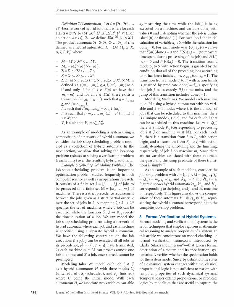
Example 6 (Job-shop Scheduling Problem): The job-shop scheduling problem is an important optimization problem studied frequently in both computer science as well as in operations research. It consists of a finite set J = {j

1, …, j

n} of jobs to

be processed on a finite set M = {m1, …, m

k} of

machines. There is a strict precedence requirement between the jobs given as a strict partial order ≺ over the set of jobs in J. A mapping ζ : J → 2M specifies the set of machines where a job can be executed, while the function δ : J → R≥0

specify the time duration of a job. We can model the job-shop scheduling problem using a network of hybrid automata where each job and each machine is specified using a separate hybrid automaton. We have the following constraints on the job execution: i) a job j can be executed iff all jobs in its precedence, j↓ = {j′ : j′ ≺ j}, have terminated; 2) each machine m ∈ M can process atmost one job at a time; and 3) a job, once started, cannot be preempted.

Modeling Jobs. We model each job ji ∈ J

as a hybrid automaton Hi with three modes U

i

(unscheduled), Si (scheduled), and F

i (finished)

where Ui being the initial mode. With each

automaton Hi we associate two variables: variable

xi, measuring the time while the job j

i is being

executed on a machine; and variable donei with

values 0 and 1 denoting whether the job is unfin-ished (0) or finished (1). For each job j

i the initial

valuation of variable xi is 0, while the valuation for

donei = 0. For each mode m ∈ {U

i, S

i, F

i} we have

that F(m)(donei) = 0 and F(S

i)(x

i) = 1 (to measure

time spent during processing of the job) and F(Ui)

(xi) = 0 and F(F

i)(x

i) = 0. The transition from a

mode Ui to S

i with action begin

i is guarded by the

condition that all of the preceding jobs according to ≺ has been finished, i.e. ∧ =:k k i k≺ ( )done 1 . The transition from a mode S

i to F

i with action finish

i

is guarded by predicate done′ =i ijδ ( ) specifying that job j

i takes exactly δ(j

i) time units, and the

jump of this transition includes done′ =j 1.Modeling Machines. We model each machine

mi ∈ M using a hybrid automaton with no vari-

able and k + 1 modes where k is the number of jobs that can be scheduled to this machine: there is a unique mode I

i (idle), and for each job j

j that

can be scheduled to this machine, i.e. mi ∈ ζ(j

i)

there is a mode Pi,j (corresponding to processing

job jj ∈ J on machine m

i ∈ M). For each mode

Pi,j there is a transition from I

i to P

i,j with action

beginj and a transition from P

i,j to I

i with action

finishj denoting the scheduling and the finishing,

respectively, of job jj on machine m

i. Since there

are no variables associated with these automata the guard and the jump predicate of these transi-tions is simply .

As an example of such modeling, consider the job-shop problem with J = {j

1, j

2}, M = {m

1}, ζ(j

1)

= ζ(j2) = m

1, j

1 ≺ j

2, and δ(j

1) = 3 and δ(j

2) = 4.

Figure 8 shows hybrid automata Hj1, H

j2, and H

m1

corresponding to the jobs j1 and j

2, and the machine

m1 respectively. This figure also shows the compo-

sition of these automata Hj1 ⊗ H

j2 ⊗ H

m1 repre-

senting the hybrid automata corresponding to the complete job-shop problem.

3 Formal Verification of Hybrid SystemsFormal modeling and verification of systems is the set of techniques that employ rigorous mathemati-cal reasoning to analyze properties of a system. In this article we concentrate on model checking—a formal verification framework introduced by Clarke, Sifakis and Emerson47—that, given a formal description of a system and its specification, sys-tematically verifies whether the specification holds for the system model. Since, by definition the states of a dynamical system changes with time, classical propositional logic is not sufficient to reason with temporal properties of such dynamical systems. Temporal logics extend propositional or predicate logics by modalities that are useful to capture the



change of behaviour of a system over time. Manna and Pnueli1,77 were the first one to propose and pro-mote the use of temporal logic to specify properties of dynamical systems in the context of system veri-fication. Linear temporal logic (LTL),77 computation tree logic (CTL) and its generalization CTL*,50,77 and modal µ-calculus53 are some of the popular temporal logics used for the system specification. Timed and weighted extensions of these logics e.g. metric temporal logics (MTL and MITL),83 dura-tion calculus (DC),43 and weighted logics31,37 have also been proposed to specify more involved quan-titative properties of hybrid dynamical systems.

In this article we limit the discussion to simple qualitative properties of hybrid systems that broadly can be classified into the following two categories:76

– The reachability or guarantee properties, that ask whether the system can reach a configuration satisfying certain property p? (symbolically, we write ◊p and we say eventually p); and

– The safety properties that ask whether the sys-tem can stay forever in configurations satisfy-ing certain property p? (symbolically, we write p and we say always or globally p).

The linear temporal logic, LTL, provides a for-mal language to specify more involved nesting of such properties with ease. We begin this section (Section 3.1) by introducing Kripke structures that provide a way to mark states of the hybrid automata with properties of interest, and present the syntax and semantics of LTL that are inter-preted over Kripke structures. In Section 3.2 we formally introduce LTL model-checking problem for hybrid automata, and show that in general this

problem is undecidable. On a positive note, in Sec-tion 3.3, we show that LTL model-checking can be algorithmically solved for finite Kripke structures. Finally, in Section 3.4 we introduce the notion of bisimulation, and show that the existence of a finite bisimulation implies the decidability of LTL model-checking problem.

3.1 Hybrid Kripke structures and linear temporal logic

The formal specification of the underlying system begins by identifying key properties of interests (called atomic propositions) regarding the states of the system under verification. Kripke structures provide a way to label the states of state-transition graphs with such atomic propositions, and the linear temporal logic specifies properties of the sequence of the truth values of these propositions, called traces, for the runs of corresponding tran-sition system. Hence, before we introduce linear temporal logic LTL we need to introduce Kripke structures and their corresponding hybrid exten-sion, and the concept of traces.

Defintion 8 (Hybrid Kripke Structure): A Kripke Structure is a tuple (T, P, L) where:

– T = (S, S0, Σ, ∆) is a state transition graph,

– P is a finite set of atomic propositions, and– L : S → 2P is a labeling function that labels

every state with a subset of P.

Similarly, we define a Hybrid Kripke Structure as a tuple (H, P, L) where:

– H = (M, M0, Σ, X, ∆, I, F, V

0) is a hybrid

automaton,– P is a finite set of atomic propositions, and

Figure 8: Network of hybrid automata Hj1, Hj1, and Hm1 corresponding to jobs j1 and j2, and a machine m1, and their product automata Hj1 ⊗ Hj2 ⊗ Hm1.



– L : M → 2P is a labeling function that labels every mode with a subset of P.

Observe that the semantics of a hybrid Kripke structure is a Kripke structure.

Let us fix a hybrid Kripke structure (H, P, L) and its semantics Kripke structure (H, P, L) for the rest of this section. When the set of proposi-tions and labeling function is clear from the con-text, we use the terms state transition graph and Kripke structure, and the terms hybrid Kripke structure and hybrid automaton interchangeably.

Given a hybrid Kripke structure (H, P, L) and an infinite run r = ⟨(m

0, v

0), (t

1, a

1), (m

1, v

1), …,

(mn, v

n),…⟩ of H, we define a trace corresponding

to r, denoted as Trace(r), as the sequence ⟨L(m0),

L(m1), L(m

2),…L(m

n),…⟩. Let Trace(H, P, L) be

the set of traces of the Hybrid Kripke Structure H. For a trace σ = ⟨P

0, P

1, …, P

n, …⟩ ∈ Trace(H, P, L)

we write σ[i] = ⟨Pi, P

i + 1

, …,⟩ for the suffix of the trace starting at the index i ≥ 0.

Now we are in a position to define the syntax and semantics of linear temporal logic.

Definition 9 (Linear Temporal Logic (Syntax)): The set of valid LTL formulas over a set P of atomic propositions can be inductively defined as the following:

– and ⊥ are valid LTL formulas;– if p ∈ P then p is a valid LTL formula;– if φ and ψ are valid LTL formulas then so are

¬φ, φ ∧ ψ and φ ∨ ψ;– if φ and ψ are valid LTL formulas then so are

○φ, ◊φ, φ and φ Uψ.

We often use φ ⇒ ψ as a shorthand for ¬φ ∨ ψ. Before we define the semantics of LTL formula formally, let us give an informal description of the temporal operators ○, ◊, , and U. LTL formu-las are interpreted over traces of (Hybrid) Kripke structures. The formula ○φ, read as next φ, holds for a trace σ = ⟨P

0, P

1, P

2, …⟩ if ψ holds for the

trace σ [1]. The formula ◊φ, read as eventually φ, holds for a trace σ = ⟨P

0, P

1, P

2, …⟩ if there exists

i ≥ 0 such that the formula ψ holds for the trace σ[i]. The formula φ, read as globally or always φ, holds for a trace σ = ⟨P

0, P

1, P

2, …⟩ if for all i

≥ 0 the formula ψ holds for traces σ[i]. Finally, the formula φ U ψ, read as φ until ψ, holds for a trace σ = ⟨P

0, P

1, P

2, …⟩ if there is an index i such that

ψ holds for the trace σ[i], and for every index j before i the formula φ holds for the trace σ[j], i.e the formula φ holds until formula ψ holds.

Definition 10 (Linear Temporal Logic (Seman-tics)): For a trace σ = ⟨P

0, P

1, P

2, …⟩ of a (Hybrid)

Kripke structure we write σ |= φ to say that the trace σ satisfies the formula φ. The satisfaction of LTL formulas is defined as follows:

– σ and σ / ⊥ ;– σ p if p ∈ P

0;

– σ φ¬ if σ φ/ ;– σ φ ∧ψ if σ φ and σ ψ;– σ φ ∨ψ if σ φ or σ ψ;– σ φ○ if σ φ[ ]1 ;– σ φ ◊ if there exists i ≥ 0 such that σ φ[ ]i ;– σ φ if for all i ≥ 0 we have that σ φ[ ]i ;

and– σ φ Uψ if there exists i ≥ 0 such that σ [ ]i ψ,

and for all 0 ≤ j < i or σ φ[ ]j .

For a (hybrid) Kripke structure (H, P, L), and an LTL formula φ we say that ( )H , ,P L φ if for all σ ∈ Trace(H, P, L) we have that σ φ .

Lamport72 observed that most of the system specifications can be classified in safety properties (something will not happen) and liveness proper-ties (something must happen). Manna and Pnueli76 further refined the class of specifications starting from reachability and safety properties to intro-duce a hierarchy of temporal properties using nesting of LTL operators, for instance

– The recurrence properties that ask whether the system can infinitely often visit configurations satisfying certain property p? (symbolically, we write ◊p and we say infinitely often p); and

– The persistence properties that ask whether the system visits configurations not satisfying a certain property p only finitely often? (sym-bolically, we write ◊p and we say eventually always p).

Some examples for expressing reachability, safety, and liveness properties using LTL are shown in the following example.

Example 7: As an example let us write LTL specifications for an elevator serving k different floors. Let op

i, fl

i and req

i be atomic propositions

representing the situations that “the door at floor i is open”, “the lift is at floor i and is not moving” and “there is a request for the lift to move to the ith floor” respectively. The following are some specifi-cations in English and their LTL counterparts:

1. Reachability property: The lift will visit the ground floor sometime.

φ1 0

deffl= .◊



2. Safety property: The door of the lift is never open at a floor if the lift is not present there.

φ20

def

i

k

i ifl op==

¬ ⇒ ¬

. ∧ ( )

3. Recurrence property: The lift keeps coming back to the ground floor.

φ3 0 0 0

def

fl fl fl= ¬ ⇒ ∧ .( ) ◊ ◊

4. Persistence property: Eventually always a requested floor will be eventually served.

φ40

def

i

k

i ireq fl= ∧ ⇒

.=

◊ ◊ ( )

We refer the reader to22,50,76,77 for a detailed overview of LTL for system specification.

3.2 LTL model checking for hybrid automata

LTL model-checking problem for hybrid automata can be formally stated in the following manner.

Definition 11 (LTL Model-Checking): Given a system modeled as a (Hybrid) Kripke struc-ture (H, P, L), and a specification written as an LTL formula φ, the LTL model-checking problem is to decide whether all traces of H satisfy φ, i.e. ( )H , ,P L φ . Moreover, if the system does not sat-isfy the property give a counterexample (run of the system) violating the property.

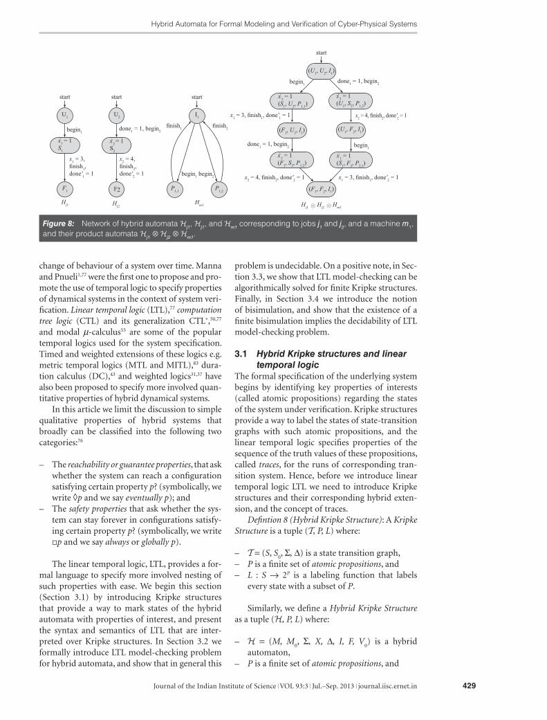
Example 8: Consider the Kripke structure T shown in Figure 9 with set of atomic propositions {p, q}. We are depicting the labeling function by writing the set of propositions inside the state, and we omit other non-relevant details. Let us consider the LTL formulas φ

1 = ◊(p ∧ ¬q) and φ

2 =

q∨ ◊p. Observe that T / φ1 as is clear from the counterexample r = ⟨m

0, a, m

1, a, m

0, …⟩ as it never

visits the configuration satisfying (p ∧ ¬q) as is clear from its trace Trace(r) = {q}{p, q} {q} {p, q}. On the other hand, it is easy to verify that T satis-fies φ

2 as any run of T either never visits m

2 (and in

that case satisfies q, or it eventually visits m2 and

never leaves it (and thus satisfies ◊p).Example 9 (Job-Shop Scheduling Revisited):

Consider the job-shop scheduling problem mod-eled as a network of hybrid automata in Fig-ure 8. Consider the atomic propositions j

1.finish

and j2.finish that are true only in modes F

1 and

F2. The counterexample produced in model-

checking LTL property ¬(◊(j1.finish ∧ j

2.finish))

gives a valid schedule for the job-shop scheduling problem.

Next, we show that LTL model-checking prob-lem for hybrid Kripke structures is undecidable. To prove this result, we show a reduction from a well-known undecidable problem of reachability (halting) for two-counter Minsky machines.81

A Minsky machine A is a tuple (L, C) where: L = {

0,

1, …,

n} is the set of instructions. There is a

distinguished terminal instruction n called HALT.

C = {c1, c

2} is the set of two counters; the instruc-

tions L are one of the following types:

1. (increment c) i : c = c + 1; goto

k,

2. (test-and-decrement c) i : if (c > 0) then

(c = c – 1); goto k else goto

m,

3. (Halt) n : HALT.

where c ∈ C, i,

k,

m ∈ L.

A configuration of a Minsky machine is a tuple (, c, d) where ∈ L is an instruction, and c, d are natural numbers that specify the value of counters c

1 and c

2, respectively. The initial configuration is

(0, 0, 0 ). A run of a Minsky machine is a (finite

or infinite) sequence of configurations ⟨k0, k

1, …⟩

where k0 is the initial configuration, and the relation

between subsequent configurations is governed by transitions between respective instructions. The run is a finite sequence if and only if the last con-figuration is the terminal instruction

n. Note that

a Minsky machine has exactly one run starting from the initial configuration. The halting prob-lem for a Minsky machine asks whether its unique run ends at the terminal instruction

n. It is well

known81 that the halting problem for two-counter Minsky machines is undecidable.

Theorem 3: The LTL model-checking problem for hybrid Kripke structures is undecidable.

Proof. Given a two counter machine A, we con-struct a hybrid Kripke structure H and an LTL for-mula φ such that Hφ iff A halts. The modes of H are labeled with the labels l

i of instructions. There

is a unique mode of H labeled with atomic propo-sition “HALT” which corresponds to the terminal instruction of A. The increment, decrement and test instructions are encoded by suitable modules

Figure 9: A Kripke structure T.



in H. The variables of H are X = {x1, x

2, y, z, z

1} with

F(m) for all modes is defined as the following:

x x y z z1 2 11 1 1 1 2= ∧ = ∧ = ∧ = ∧ = .

The initial mode is labeled by l0, the label of the

first instruction. The values of the counters c, d are encoded as x c1

12

= and x d21

2= . After the execu-

tion of each instruction, x1, x

2 will contain the cur-

rent values of counters c, d encoded in the above form. For instance, if we have x xc d1

12 2

12

= =, before incrementing counter c, then at the end of simulating the increment instruction, we will have x c1

12 1= + and x d2

12

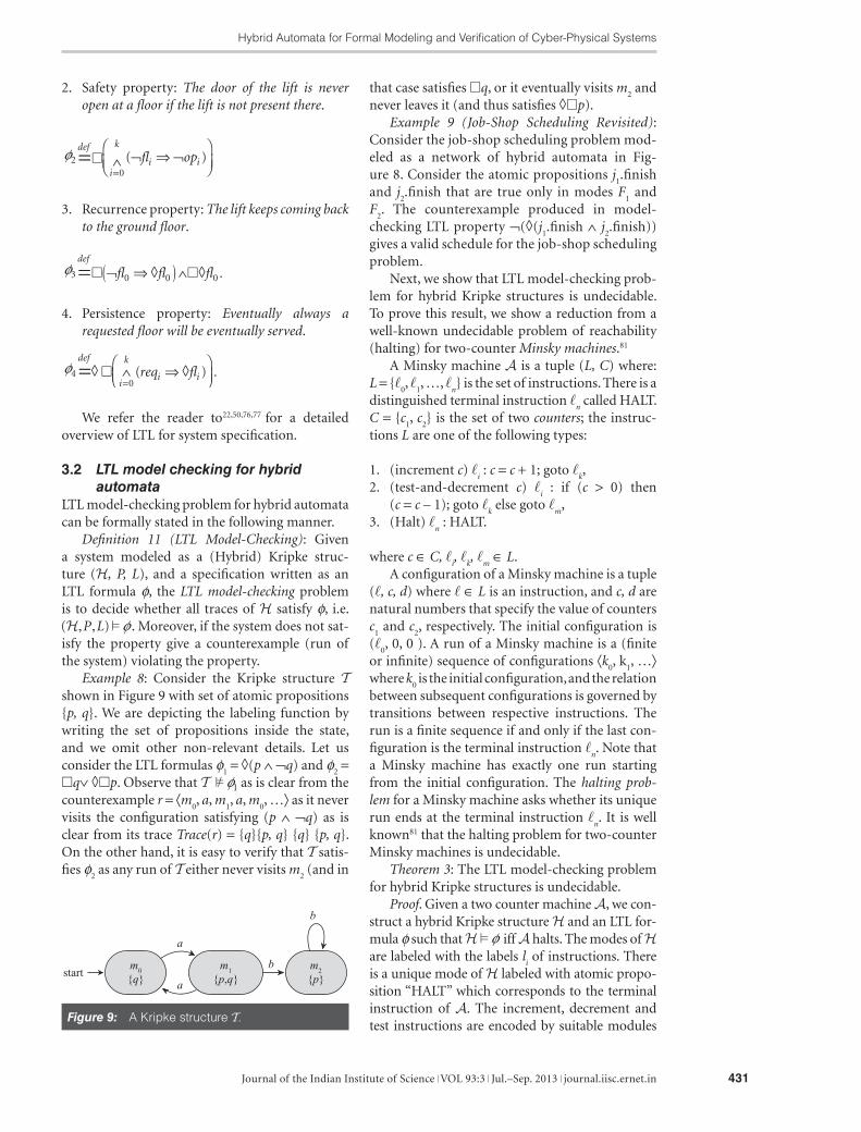
= .In Figure 10, we illustrate the case of the incre-

ment instruction li : increment c and goto l

j. The

case for the decrement instruction is similar, and hence omitted. Mode l

i is entered with y = 0,

x c112

= and x d21

2= . On entering mode A

i, we have

x y x xc d c c112 2

12

12 2

12

1 1 1 1= , = − , = + − = − −( ) or η

if 12

12

1 1d c+ = ≤ −η η, and z = 0. Mode Bi

can be entered if x2, y < 1 and x

1 > 1. Assume

k > 0 units of time was spent at mode Ai. This

gives y k x kc d c= − + , = + − +1 112 2

12

12

( ) (or 1 1

2− − +c kη , or 1 – η′ if 1 11

2− − + ′ =c η η , η′ ≤ k),

z = k, x1 = 0, z

1 =0 on entering mode B

i. We can

reach mode lj only if the values of z and

z1 are the same. Assume l units of time

was spent at Bi. Then z = k + l, z

1 = 2l,

x k l x l y k ld c c21

212 1

12

1 1= + − + + , = , = − + +( ) . To

satisfy the constraints z = z1, y = 1, we have k = 1 and

k l k c+ = =2 12

giving x xc d11

2 21

21= , =+ , y = 0 at lj.

The LTL formula φ = l0 ∧ ◊ HALT will be satisfied

by H iff A halts. This shows that LTL model check-ing of hybrid Kripke structures is undecidable.

3.3 LTL model-checking for finite Kripke structures

As we discussed in previous section the LTL model-checking problem is undecidable for general hybrid automata. However, for finite Kripke structures Wolper, Vardi, and Sistla99 developed an elegant automata-theoretic algorithm for solving the LTL model-checking problem. The algorithm exploits the connection between LTL formulas and a type of ω-automata—automata that extend the theory of finite automata to infinite inputs—called Büchi

automata.40,56 The syntax for the Büchi automata specifies a finite state transition graph T along with a set F of accepting states, and the semantics of Büchi automata restricts the set of valid runs to the runs of T that visit F infinitely often. In general Büchi automata are closed under all Boolean oper-ations including union, intersection, and comple-mentation, however deterministic variant of Büchi automata is not closed under complementation. Emptiness checking for Büchi automata can be decided efficiently (linear in time) by analyzing strongly connected components of T.

The LTL model-checking problem exploits the following connection between linear temporal logic and Büchi automata.

Theorem 4 (LTL-to-Büchi Automata):99 For every LTL formula φ we can effectively construct a finite (Büchi) automaton Aφ (of size exponential in φ) such that words recognized by Aφ are pre-cisely the set of traces that satisfy φ.

Based on this result, the LTL model checking for a finite Kripke structure K can be performed in the following manner:

1. Construct a Büchi automaton A¬φ correspond-ing to the negation of the LTL property.

2. Construct the composition K⊗A¬φ of the Kripke structure K with the Büchi automaton A¬φ.

3. If the Büchi automaton H⊗A¬φ is empty, then return “TRUE”

4. Else, return a lasso-shaped (a finite prefix fol-lowed by a cycle that contains an accepting state) infinite run accepted by H⊗A¬φ as a counter-example.

The correctness of this algorithm follows from the observation that the set of traces for this com-position K⊗A¬φ characterize the set of traces that are generated by K that do not satisfy φ. Hence, the Kripke structure K satisfies the LTL property φ if and only if H⊗A¬φ is empty.

Theorem 5 (LTL model-Checking for Finite Structures):91 LTL model checking problem for finite Kripke structures is decidable in PSPACE.

LTL model-checking for finite Kripke struc-tures is implemented by a number of mature tools, notably SPIN92 and NuSMV,82 and has been applied to a number of practical case-studies.82,92

Figure 10: Module simulating li: increment c, goto lj .



3.4 Finite bisimulation and decidabilityIn this section we introduce the concept of bisimu-lation relation between two Kripke structures, and show that for two bisimilar systems (systems hav-ing a bisimulation relation between their states) we have that both systems have the same set of traces, and hence precisely the same set of LTL formulas are satisfied by both of them. Using this idea, we show that if for a given hybrid Kripke structure H there exists a bisimulation relation with some finite state Kripke structure K, then the problem of LTL model-checking for H can be reduced to the decidable problem of LTL model-checking for finite Kripke structure K.

We say that a Kripke structure ′ = ′, , ′K T( )P L can simulate a Kripke structure K = (T, P, L) if every step of K can be matched (with respect to atomic propositions) by one or more steps of K′. A Bisimulation equivalence denotes the presence of a mutual simulation between two structures K and K′. Formally, bisimulation relation is defined in the following manner.

Definition 12 (Bisimulation Relation): Let K = (T = S, S

0, Σ, ∆), P, L) and ′ = =K T(

( ) )′, ′ , ′, ′∆ , , ′S S P L0 Σ be two Kripke structures. A bisimulation relation between K and K′ is a binary relation R ⊆ S × S′ such that:

– every initial state of T is related to some initial state of T′, and vice-versa, i.e. for every s ∈ S

0

there exists ′ ∈ ′s S0 such that (s, s′) ∈ R and for every ′ ∈ ′s S0 there exists a s ∈ S

0 such that (s,

s′) ∈ R;– for every (s, s′) ∈ R the following holds:

– L(s) = L′ (s′),– every outgoing transition of s is matched

with some outgoing transition of s′, i.e. if t ∈ Post(s) then there exists t′ ∈ Post(s′) with (t, t′) ∈ R, and

– every outgoing transition of s′ is matched with some outgoing transition of s, i.e. if t′ ∈ Post(s′) then there exists t ∈ Post(s) with (t, t′) ∈ R.

We say that T and T ′ (analogously, K and K′) are bisimilar or bisimulation equivalent, and we write T ∼ T ′, if there exists a bisimulation relation R ⊆ S × S′.

The following Proposition follows from the def-inition of bisimulation and the semantics of LTL.

Proposition 6: If T ∼ T ′ then Trace(T ) = Trace(T ′). Moreover, if T ∼ T ′ then for every LTL formula φ we have that T φ if and only if

′T φ .Proof. Let T ∼ T ′. Using a simple inductive argu-

ment, one can show that for every run a = ⟨s0, a

1,

s1, a

2, …⟩ of T there is a run ′ = ′ , ′, ′, ′ ,r s a s a⟨ ⟩0 1 1 2 ...

of T ′ such that L s L si i( ) ( )= ′ ′ for every i ≥ 0. This implies that Trace(r) = Trace(r ′) and hence Trace(T ) ⊆ Trace(T ′). Similarly, we can show that Trace(T ′) ⊆ Trace(T). Hence it follows that T ∼ T ′ implies Trace(T) = Trace(T ′). To prove the other part of the proposition, observe LTL formulae are interpreted over traces of structures, and since two bisimilar Kripke structures have the same set of traces, it follows that for every LTL formula φ we have that T ∼ T ′ implies that T φ if and only if

′T φ . This proposition shows that LTL model check-

ing problem can be reduced to solving LTL model checking problem over a bisimilar Kripke struc-ture. We next show how to extend this idea to define bisimulation over the states of a Kripke structure, and use it to produce a bisimilar Kripke structure with fewer states.

Definition 13 (Bisimulation Relation on K): Let K = (T = (S, S

0, Σ, ∆), P, L) be a Kripke structure. A

bisimulation on K is a binary relation R ⊆ S × S such that for all (s, s′) ∈ R we have that:

– L(s) = L(s′);– if t ∈ Post(s), then there exists an t′ ∈ Post(s′)

such that (t, t′) ∈ R;– if t′ ∈ Post(s′), then there exists an t ∈ Post(s)

such that (t, t′) ∈ R.

It is easy to see that a bisimulation relation R over the state space of K is an equivalence relation. For a state s ∈ S we write [s]

R for the equivalence

class of R containing s. We say that states s, s′ ∈ S are bisimulation equivalent, and we write s ∼

T s′,

if there exists a bisimulation relation R for T with (s, s′) ∈ R.

Given a Kripke structure T, we use a bisimula-tion relation R for reducing the state space of T using the following quotient construction.

Definition 14 (Bisimulation Quotient): Given a Kripke structure K = (T = (S, S

0, Σ, ∆), P, L) and a

bisimulation relation R ⊆ S × S over K, the bisimu-lation quotient K

R is defined as a Kripke structure

K TR R R R R R R= = , ∆ , ,( ( , , ) )S S P L0 Σ where:

– The state space of TR

is the quotient space of T, i.e. S

R = {[s]

R: s ∈ S};

– The set of initial states is the set of R-equivalence classes of the initial states, i.e. S s s SR R

00= : ∈{[ ] };

– ∑R

= {t};

c Observe that the definition of bisimulation ensures that the

state labeling LR

is well defined.



– Each transition (s, a, s′) ∈ ∆ induces a transition from [s]

R to [s′]

R in ∆

R, i.e.

∆R R R= , ′ : , , ′ ∈∆{([ ] , [ ] ) ( ) }s s s sτ α , and– L

R is defined such that L

R([s]) = L(s)c.

We say that a bisimulation quotient is finite if there are finitely many equivalence classes of R, i.e. |S

R| < ∞.

The proof of the following theorem is imme-diate from Proposition 6 and Theorem 5.

Theorem 7: The existence of a finite bisimula-tion quotient for a hybrid Kripke structure imply the decidability of LTL model-checking problem.

4 Decidable Subclasses of Hybrid Automata

Given the expressiveness of hybrid automata it is not surprising that simple reachability questions are undecidable for general hybrid kripke struc-tures. In this section we discuss some prominent subclasses of hybrid automata for which LTL model checking problem is decidable. In the pre-vious section we discussed that showing the exist-ence of a finite bisimulation quotient guarantees decidable model-checking. Timed automata were among the first hybrid automata shown to have decidable model-checking using this approach. We begin this section by presenting timed autom-ata and discuss this bisimulation known as region-equivalence relation. We will also review multi-rate and rectangular hybrid automata (Section 4.2) that under certain restriction (initialized) recover decidability of LTL model-checking via reductions to similar problem on timed automata. Finally, in Section 4.3 we discuss a relatively simple class of hybrid systems, called piecewise-constant deriva-tive systems, that capture the essence of undecid-ability and provide references to its variants that permit algorithmic analysis.

4.1 Timed automataTimed automata, introduced by Alur and Dill,10,11 is a popular formalism to model real-time systems. A timed automaton is a hybrid automaton where all variables grow with a constant and uniform rate (for all variables x ∈ X we have that x = 1) and the only jump permitted during the discrete transitions is reset to zero. Moreover, the set of predicates permitted to appear as guard on transi-tions is restricted to the following kind of octago-nal predicates:

g x c x y c g g: = | − | ∧ (4)

where x, y are clock variables, ∈ <,≤,=,>,≥{ } and c ∈ N. We write Z(X) for this class of octagonal

predicates over the set X. Formally, we define a timed automata as a restriction of hybrid autom-ata in the following manner.

Definition 15 (Timed Automata: Syntax): A timed automaton is a hybrid automaton T = (M, M

0, ∑, X, ∆, I, F, V

0) with the following

restrictions:

– The transition relation ∆ ⊆ M × pred(X) × ∑ × pred(X ∪ X′) × M is such that if (m, g, a, j, m′) ∈ ∆ then– the guard g is of the form (4), i.e. g ∈ Z(X)

and– the jump predicate j only permits variable

resets to zero, i.e. j is of the form

∧ ′ = ,∈x Y x( )0

for some Y ⊆ X. We denote such set Y as reset(j).

– The mode-invariant function I : M → pred(X) is such that for all m ∈ M we have that I(m) ∈ Z(X);

– The flow function F : M → (R|X| → R|X|) is such that for all m ∈ M we have that F(m) characterizes:

∧ = ,∈x X x( ) 1 and

– V0 ∈ pred(X) is the set of initial valuations is

such that V xx X0 0= ∧ =∈ ( ).

The semantics of timed automata and the concept of timed Kripke structures is defined in a similar way as for hybrid automata.

Example 10: The hybrid automaton correspond-ing to the job-shop scheduling problem, shown in Figure 8, can also be modeled as a timed automa-ton by requiring that the rates of variables x

1 and

x2 is 1 in all the modes (unlike the current example

where these clocks are paused in certain modes).Example 11: As an example of a timed automa-

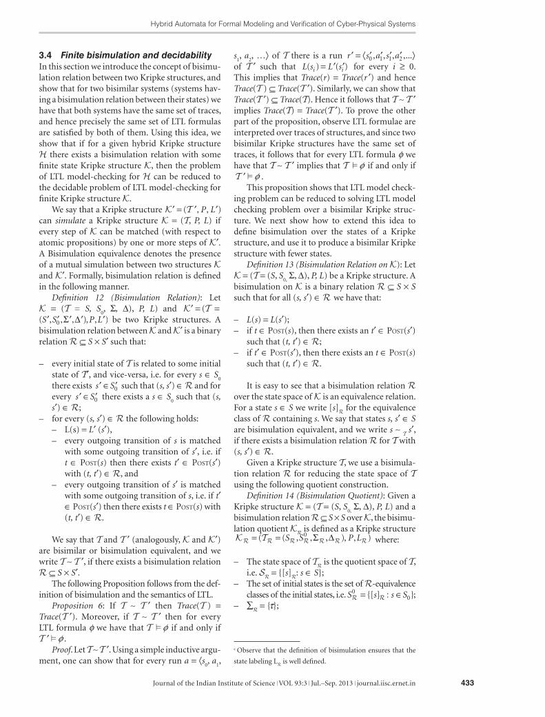
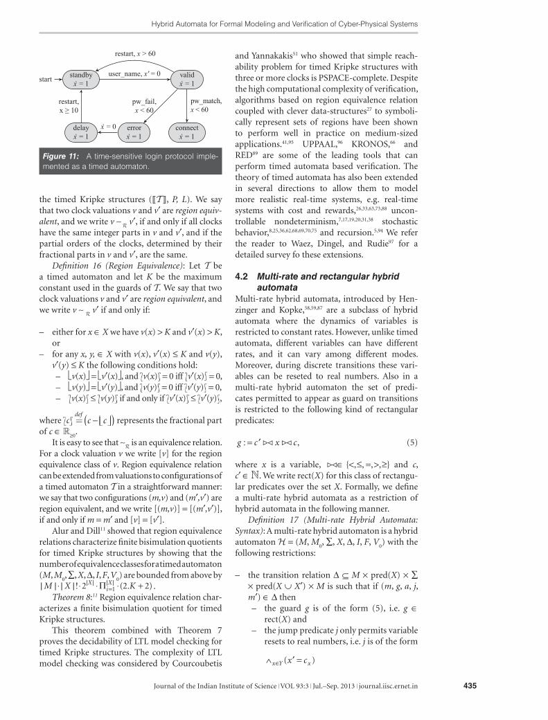
ton consider Figure 11 that models a login pro-tocol using a timed automaton. The system starts in the “standby” mode. If the user gives a correct password within 60 time-units after giving the user name, a connection will be established; if, however, the password given is wrong, the sys-tem restarts after a delay of at least 10 time units. Moreover, if no password is given within 60 time units after supplying user name, then the system restarts in the standby mode. This system is mod-eled using a timed automaton with five modes and one clock in Figure 11.

Alur and Dill11 proposed the notion of region equivalence to define a bisimulation relation over



the timed Kripke structures (T , P, L). We say that two clock valuations v and v′ are region equiv-alent, and we write v ∼

R v′, if and only if all clocks

have the same integer parts in v and v′, and if the partial orders of the clocks, determined by their fractional parts in v and v′, are the same.

Definition 16 (Region Equivalence): Let T be a timed automaton and let K be the maximum constant used in the guards of T. We say that two clock valuations v and v′ are region equivalent, and we write v ∼

R v′ if and only if:

– either for x ∈ X we have v(x) > K and v′(x) > K, or

– for any x, y, ∈ X with v(x), v′(x) ≤ K and v(y), v′(y) ≤ K the following conditions hold:– v(x) = v′(x), and v(x) = 0 iff v′(x) = 0,– v(y) = v′(y), and v(y) = 0 iff v′(y) = 0,– v(x) ≤ v(y) if and only if v′(x) ≤ v′(y) ,

where c =def

c c− ( ) represents the fractional part of c ∈ R≥0

.It is easy to see that ∼

R is an equivalence relation.

For a clock valuation v we write [v] for the region equivalence class of v. Region equivalence relation can be extended from valuations to configurations of a timed automaton T in a straightforward manner: we say that two configurations (m,v) and (m′,v′) are region equivalent, and we write [(m,v)] = [(m′,v′)], if and only if m = m′ and [v] = [v′].

Alur and Dill11 showed that region equivalence relations characterize finite bisimulation quotients for timed Kripke structures by showing that the number of equivalence classes for a timed automaton (M, M

0, ∑, X, ∆, I, F, V

0) are bounded from above by

| | ⋅ | |!⋅ ⋅ ⋅ . +| |=

| |M X KXiX2 2 21Π ( ) .

Theorem 8:11 Region equivalence relation char-acterizes a finite bisimulation quotient for timed Kripke structures.

This theorem combined with Theorem 7 proves the decidability of LTL model checking for timed Kripke structures. The complexity of LTL model checking was considered by Courcoubetis

and Yannakakis51 who showed that simple reach-ability problem for timed Kripke structures with three or more clocks is PSPACE-complete. Despite the high computational complexity of verification, algorithms based on region equivalence relation coupled with clever data-structures27 to symboli-cally represent sets of regions have been shown to perform well in practice on medium-sized applications.41,95 UPPAAL,96 KRONOS,66 and RED89 are some of the leading tools that can perform timed automata based verification. The theory of timed automata has also been extended in several directions to allow them to model more realistic real-time systems, e.g. real-time systems with cost and rewards,26,33,63,73,88 uncon-trollable nondeterminism,7,17,19,20,31,38 stochastic behavior,8,25,36,62,68,69,70,75 and recursion.5,94 We refer the reader to Waez, Dingel, and Rudie97 for a detailed survey fo these extensions.

4.2 Multi-rate and rectangular hybrid automata

Multi-rate hybrid automata, introduced by Hen-zinger and Kopke,58,59,87 are a subclass of hybrid automata where the dynamics of variables is restricted to constant rates. However, unlike timed automata, different variables can have different rates, and it can vary among different modes. Moreover, during discrete transitions these vari-ables can be reseted to real numbers. Also in a multi-rate hybrid automaton the set of predi-cates permitted to appear as guard on transitions is restricted to the following kind of rectangular predicates:

g c x c: = ′ , (5)

where x is a variable, ∈ <,≤, =,>,≥{ } and c, c′ ∈ N. We write rect(X) for this class of rectangu-lar predicates over the set X. Formally, we define a multi-rate hybrid automata as a restriction of hybrid automata in the following manner.

Definition 17 (Multi-rate Hybrid Automata: Syntax): A multi-rate hybrid automaton is a hybrid automaton H = (M, M

0, ∑, X, ∆, I, F, V

0) with the

following restrictions:

– the transition relation ∆ ⊆ M × pred(X) × ∑ × pred(X ∪ X′) × M is such that if (m, g, a, j, m′) ∈ ∆ then– the guard g is of the form (5), i.e. g ∈

rect(X) and– the jump predicate j only permits variable

resets to real numbers, i.e. j is of the form

∧ ′ =∈x Y xx c( )

Figure 11: A time-sensitive login protocol imple-mented as a timed automaton.



where Y ⊆ X and cx ∈ Z for each x ∈ Y.

We denote such set Y as reset(j).– the mode-invariant function I : M → pred(X)

is such that for all m ∈ M we have that I(m) ∈ rect(X);

– the flow function F : M → (R|X| → R|X|) is such that for all m ∈ M we have that F(m) characterize:

∧ = ,∈ ,x X x mx c( )

where cx,m

∈ Z for each x ∈ X; and– V

0 ∈ pred(X) is the set of initial valuations is

such that V xx X0 0= ∧ =∈ .

The semantics of multi-rate automata and the concept of multi-rate Kripke structures is defined is a similar way as for hybrid automata. Rectangular hybrid automata58,59 are a generaliza-tion of multi-rate hybrid automata where within each mode the rate of a variable can change non- deterministically within a given mode-dependent interval.

Using a reduction from two counter Minsky machine, one can easily show that the LTL model checking problem for multi-rate hybrid automata is undecidable.

Theorem 9:59 LTL model-checking problem for multi-rate hybrid automata is undecidable.

We say that a multi-rate (or rectangular) hybrid automaton is initialized if it satisfies the property that every transition between two modes with different rates (rate intervals, resp.) for a var-iable, resets that variable, i.e. for every transition (m, g, a, j, m′) ∈ ∆ with F(m)(x) ≠ F(m′)(x) we have x ∈ reset(j). Figure 12 shows an initialized rectangular automaton.

Henzinger et al.59 showed the decidability of initialized rectangular and multi-rate hybrid automata.

Theorem 10: The LTL model-checking prob-lem for initialized rectangular (multi-rate) hybrid automata is decidable.

Proof. The decidability of LTL model-check-ing problem for initialized multi-rate automata by reducing the problem to similar problem for timed automata by rescaling the rate of all vari-ables to one via appropriate adjustment of the constraints on the mode invariants and guards in all the transitions.

To prove the decidability for an initialized rectangular automaton H

r, we reduce the prob-

lem to corresponding problem for an initialized multi-rate automaton H

m. Each variable x of H

r

with rate in the rectangle a x b≤ ≤ is simulated using two variables x

l, x

u such that x al = and

x bu = . The variables xl, x

u keep track of the lower

and upper bounds of x respectively. With this replacement, the invariant conditions of modes, as well as guards and resets on transitions have to be adjusted appropriately. For example, if we had a transition with guard x ≤ 10, then it is replaced with (i) x

l ≤ 10 and (ii) x xu u> , ′ =10 10 . This con-

version from initialized rectangular to initialized multirate automata is language preserving. Hence, from the decidability of LTL model checking prob-lem for initialized multi-rate hybrid automata, the decidability for initialized rectangular hybrid follows.

4.3 Piecewise-constant derivative systems and their variants

Asarin, Maler, and Pnueli18 initiated the study of hybrid dynamical systems with piecewise-constant derivatives (PCD) defined as a partition of the Euclidean space into a finite set of regions (polyhedral predicates), where the dynamics in a region is defined by a constant rate vector. They defined PCD systems as completely determin-istic systems where a discrete transition occurs at region boundaries, where runs change their directions according to the rate vector available in the new region. Given the simplicity of such systems, it is perhaps surprising that the reach-ability problem for PCD systems with three or more variables is undecidable.18 In fact, Asarin and Maler16 observed that, due to the capability of such systems to perform Zeno runs, every set of arithmetical hierarchy (a hierarchy of unde-cidable problems) can be recognized by a PCD system of some finite dimension. On the positive side, Asarin, Maler, and Pnueli18 gave an algo-rithm to solve the reachability problem for two-dimensional PCD systems. Cerans and Viksna42 later generalized this decidability result to more general piecewise-Hamiltonian systems. We also mention the work of Asarin, Schneider, Yovine21 who extended the decidability result for two-di-mensional PCD systems to a non-deterministic setting of simple planar differential inclusion sys-tems (SPDIs) where a number of rate vectors are available in each region.

Kesten, Pnueli, Sifakis, and Yovine64 also studied another variant of constant-rate hybrid systems, called integration graphs, that can be considered as a subset of multi-rate automaton

Figure 12: An initialized rectangular automaton.



where no test of non-clock (integrator) variables is allowed to appear on a loop. Kesten et al.64 showed the decidability for the two subclasses of integration graphs: The class with a single clock variable, and the class where integrators are tested only once.

Recently, Bouyer et al.35 introduced timed automata with energy constraints, that can be considered as multi-rate automata with a single non-clock variable (energy variable) that does not appear on guards, and showed decidability of schedulability problem where the energy vari-able is required to be greater than a given lower-bound. Bouyer, Fahrenberg, Larsen, and Markey34 later generalized this result to give an EXPTIME algorithm for a subclass where energy variables can grow exponentially.

Alur, Trivedi, and Wojtczak recently studied constant-rate multi-mode systems,13 that can be considered as multi-rate automata with the excep-tion that there is no structure in the automata, i.e. any mode can be used after any other mode, and there is only a global invariant over variables. They showed that reachability and schedulability problems for these systems can be solved in poly-nomial time for starting states strictly inside the global invariant space. Alur, Trivedi, and Wojtczak also showed that introducing either local invari-ants or guards make the reachability problem undecidable. Alur et al.12 later studied this problem for a generalization of constant-rate multi-mode systems to bounded-rate multi-mode system and showed the decidability of the schedulability problem.

5 SummaryIn this article we presented hybrid automata for modeling and formal verification of cyber-phys-ical systems. Hybrid automata naturally combine features from continuous dynamical systems and discrete finite state machines, and provide an ele-gant and expressive model. This expressiveness, however, comes with a price—the simple reach-ability problem for simple subclasses of hybrid automata, like piecewise-constant derivative sys-tems, turned out to be highly undecidable. In this article we discussed a general approach of finding finite bisimulation quotient to show decidability of subclasses of hybrid automata, and sketched the proof for the decidability for two key sub-classes: timed automata and initialized rectangu-lar hybrid automata. Hybrid automata provide an intuitive and semantically unambiguous way to model cyber-physical systems. These formal-isms provide a rich theory and a mature set of tools, UPPAAL,96 Kronos,66 RED,89 HyTECH,60

and PHAVer,86 able to perform automatic verifi-cation of systems modeled using them. A grow-ing number of case-studies using these tools have shown promise in extending the state-of-the-art to industrial-sized examples.

Received 22 August 2013.

References 1. ACM Turing award citation for A. Pnueli. http://awards.

acm org/citation.cfm?id=4725172&srt=alpha&alpha=P&

aw=140&ao=AMTURING&yr=1996, 1996. For seminal

work introducing temporal logic into computing science

and for outstanding contributions to program and system

verification.

2. ACM Turing award citation for E.M. Clarke, E.A.

Emerson, and J. Sifakis. http://awards.acm.org/citation.

cfm?id=1167964&srt=alpha&alpha=C&aw=140&ao=A

MTURING&yr=2007, 2007. For their role in develop-

ing Model- Checking into a highly effective verification

technology, widely adopted in the hardware and software

industries.

3. ACM Kanellakis theory and practice award citation for

G.J. Holzmann, R.P. Kurshan, M.Y. Vardi, and P. Wolpe.

http://awards.acm.org/citation.cfm?id=1625680&srt

=all&aw=147&ao=KANELLAK&yr=2005, 2005. For

the development of automata-theoretic techniques for

reactive-systems verification, and the practical realiza-

tion of powerful formal-verification tools based on these

techniques.

4. ACM Kanellakis theory and practice award citation for

R.E. Bryant, E.M. Clarke, E.A. Emerson, K.L. Mcmillan.

http://awards.acm.org/citation.cfm?id=1167964&srt=a

ll&aw=147&ao=KANELLAK&yr=1998, 1998. For their

invention of “symbolic model checking”.

5. P.A. Abdulla, M.F. Atig, and J. Stenman. Dense-timed

pushdown automata. In Proceedings of the 2012 27th

Annual IEEE/ACM Symposium on Logic in Computer Sci-

ence, LICS ’12, pp. 35–44, Washington, DC, USA, 2012.

IEEE Computer Society.

6. R. Alur and M. Bernadsky. Bounded model checking for

GSMP models of stochastic real-time systems. In Proceed-

ings of HSCC, volume 3927, pp. 19–33. LNCS, 2006.

7. R. Alur, M. Bernadsky, and P. Madhusudan. Optimal reach-

ability for weighted timed games. In J. Díaz, J. Karhumäki,

A. Lepistö, and D. Sannella, editors, Proc. ICALP’04,

volume 3142 of LNCS, pp. 122–133. Springer, 2004.

8. R. Alur, C. Courcoubetis, and D.L. Dill. Model-checking for

probabilistic real-time systems. In Automata, Languages and

Programming: Proceedings of the 18th ICALP, Lecture Notes

in Computer Science 510, pp. 115–126. Springer, 1991.

9. R. Alur, C. Courcoubetis, T.A. Henzinger, and P.-H. Ho.

Hybrid automata: An algorithmic approach to the speci-

fication and verification of hybrid systems. In Hybrid

Systems I, volume 736 of Lecture Notes in Computer Science,

pp. 209–229. Springer-Verlag, 1993.



10. R. Alur and D. Dill. Automata for modeling real-time

systems. In International Colloquium on Automata, Lan-

guages and Programming (ICALP), volume 443 of LNCS,

pp. 322–335. Springer, 1990.

11. R. Alur and D. Dill. A theory of timed automata. Theoretical

Computer Science, 126: pp. 183–235, 1994.

12. R. Alur, V. Forejt, S. Moarref, and A. Trivedi. Safe schedula-

bility of bounded-rate multi-mode systems. In Hybrid Sys-

tems: Computation and Control (HSCC), pp. 243–252, 2013.

13. R. Alur, A. Trivedi, and D. Wojtczak. Optimal scheduling

for constant rate multi-mode systems. In Hybrid Systems:

Computation and Control (HSCC), pp. 75–84, 2012.

14. Rajeev Alur and Thomas A. Henzinger. Logics and models

of real time: A survey. In Real-Time: Theory in Practice,

pp. 74–106. Springer, 1992.

15. P. Argón, G. Delzanno, S. Mukhopadhyay, and A. Podelski.

Model checking communication protocols. In Proceed-

ings of the 28th Conference on Current Trends in Theory

and Practice of Informatics Piestany: Theory and Practice

of Informatics, SOFSEM ’01, pp. 160–170, London, UK,

2001. Springer-Verlag.

16. E. Asarin and O. Maler. Achilles and the tortoise climb-

ing up the arithmetical hierarchy. Journal of Computer and

System Sciences, 57(3): pp. 389–398, 1998.

17. E. Asarin and O. Maler. As soon as possible: Time optimal

control for timed automata. In F.W. Vaandrager and J.H.

van Schuppen, editors, Proc. HSCC’99, volume 1569 of

LNCS, pp. 19–30. Springer, 1999.

18. E. Asarin, O. Maler, and A. Pnueli. Reachability analysis of

dynamical systems having piecewise-constant derivatives.

Theoretical Computer Science, 138(1): pp. 35–65, 1995.

19. E. Asarin, O. Maler, and A. Pnueli. Symbolic controller

synthesis for discrete and timed systems. In P. Antsaklis,

W. Kohn, A. Nerode, and S. Sastry, editors, Hybrid Systems

II, volume 999 of LNCS, pp. 1–20. Springer, 1995.

20. E. Asarin, O. Maler, A. Pnueli, and J. Sifakis. Controller

synthesis for timed automata. In P. Antsaklis, W. Kohn, A.

Nerode, and Sastry S., editors, Proceedings of IFAC Sym-

posium on System Structure and Control, pp. 469–474.

Elsevier, 1998.

21. E. Asarin, G. Schneider, and S. Yovine. On the decid-

ability of the reachability problem for planar differential

inclusions. In Hybrid Systems: Computation and Control,

pp. 89–104. Springer, 2001.

22. C. Baier and J.-P. Katoen. Principles of Model Checking

(Representation and Mind Series). The MIT Press, 2008.

23. T. Ball, V. Levin, and S.K. Rajamani. A decade of software

model checking with SLAM. Communications of the ACM,

54(7): pp. 68–76, July 2011.

24. D. Basin, C. Cremers, and C. Meadows. Model checking

security protocols. Handbook of Model Checking, 2011.

http://people.inf.ethz.ch/cremersc/publications/index.html

25. D. Beauquier. Probabilistic timed automata. Theoretical

Computer Science, 292(1): pp. 65–84, 2003.

26. G. Behrmann, A. Fehnker, T. Hune, K.G. Larsen,

P. Pettersson, J. Romijn, and F.W. Vaandrager. Minimum-

cost reachability for priced timed automata. In M.D. Di

Benedetto and A.L. Sangiovanni-Vincentelli, editors, Proc.

HSCC’01, volume 2034 of LNCS, pp. 147–161, Heidelberg,

2001. Springer.

27. J. Bengtsson and W. Yi. Timed automata: Semantics, algo-

rithms and tools. In Lectures on Concurrency and Petri

Nets, pp. 87–124, 2003.

28. J. Berendsen, D. Jansen, and J.-P. Katoen. Probably on time

and within budget—on reachability in priced probabilis-

tic timed automata. In Proc. QEST’06, pp. 311–322, Wash-

ington, DC, USA, 2006. IEEE.

29. A. Biere, A. Cimatti, E.M. Clarke, O. Strichman, and

Y. Zhu. Bounded model checking. Advances in computers,

58: pp. 117–148, 2003.

30. A. Biere, A. Cimatti, E.M. Clarke, O. Strichman, and Y.

Zhu. Bounded model checking. Handbook of Satisfiability,

185: pp. 457–481, 2009.

31. P. Bouyer. Weighted timed automata: Model-checking and

games. Electronic Notes Theoretical Computer Science, 158:

pp. 3–17, 2006.

32. P. Bouyer, T. Brihaye, M. Jurdzinski, R. Lazic, and

M. Rutkowski. Average-price and reachability-price games

on hybrid automata with strong resets. In Formal Mod-

eling and Analysis of Timed Systems (FORMATS), volume

5215 of LNCS, pp. 63–77. 2008.

33. P. Bouyer, E. Brinksma, and K.G. Larsen. Optimal infi-

nite scheduling for multi-priced timed automata. Formal

Methods in System Design, 32(1): pp. 3–23, 2008.

34. P. Bouyer, U. Fahrenberg, K.G. Larsen, and N. Markey.

Timed automata with observers under energy constraints.

In Hybrid Systems: Computation and Control (HSCC), 2010.

35. P. Bouyer, U. Fahrenberg, K.G. Larsen, N. Markey, and

J. Srba. Infinite runs in weighted timed automata with

energy constraints. In Formal Modeling and Analysis of

Timed Systems, pp. 33–47. Springer, 2008.

36. P. Bouyer, and V. Forejt. Reachability in stochastic timed

games. In International Colloquium on Automata, Lan-

guages and Programming (ICALP), volume 5556 of LNCS,

pp. 103–114. Springer, 2009.

37. T. Brihaye, V. Bruyere, and J.-F. Raskin. Model-checking

for weighted timed automata. In Yassine Lakhnech and

Sergio Yovine, editors, Formal Techniques, Modelling and

Analysis of Timed and Fault-Tolerant Systems, volume

3253 of Lecture Notes in Computer Science, pp. 277–292.

Springer Berlin Heidelberg, 2004.

38. T. Brihaye, T.A. Henzinger, V.S. Prabhu, and J. Raskin.

Minimum-time reachability in timed games. In Proc.

ICALP’07, volume 4596 of LNCS, pp. 825–837. Springer,

2007.

39. M. Broy, I.H. Kruger, A. Pretschner, and C. Salzmann.

Engineering automotive software. Proceedings of the IEEE,

95(2): pp. 356–373, 2007.

40. J.R. Büchi. On a decision method in restricted second-

order arithmetic. In Int. Congr. for Logic Methodology and

Philosophy of Science, pp. 1–11. Standford University Press,

Stanford, 1962.



41. F. Cassez, J. Jessen, K. Larsen, J. Raskin, and P. Reynier. Auto-

matic synthesis of robust and optimal controllers: an indus-

trial case study. In F.W. Vaandrager and J.H. van Schuppen,

editors, HSCC’09, volume 5469 of LNCS, 2009.

42. K. Cerans and J. Viksna. Deciding reachability for planar

multi-polynomial systems. In Hybrid Systems, pp. 389–400,

1995.

43. Zhou Chaochen, Anders P. Ravn, and Michael R. Hansen.

An extended duration calculus for hybrid real-time systems.

In Hybrid Systems, volume 736 of Lecture Notes in Computer

Science, pp. 36–59. Springer Berlin Heidelberg, 1993.

44. Robert N. Charette. This car runs on code. http://news.

discovery.com/autos/toyota-recall-software-code.htm,

February 2013.

45. K. Chatterjee, T.A. Henzinger, and V. Prabhu. Timed par-

ity games: Complexity and robustness. In Proceedings of

the Sixth International Conference on Formal Modeling and

Analysis of Timed Systems (FORMATS’08), volume 5215 of

LNCS, pp. 124–140, 2008.

46. E.M. Clarke, E.A. Emerson, S. Jha, and A.P. Sistla. Sym-

metry reductions in model checking. In Computer Aided

Verification, pp. 147–158. Springer, 1998.

47. E.M. Clarke, E.A. Emerson, and J. Sifakis. Model checking:

algorithmic verification and debugging. Communications

of the ACM, 52(11): pp. 74–84, 2009.

48. E.M. Clarke, A. Fehnker, Z. Han, J. Krogh, B.H. and Oua-

knine, O. Stursberg, and M. Theobald. Abstraction and

counterexample-guided refinement in model checking

of hybrid systems. International Journal of Foundations of

Computer Science, 14(4): pp. 583–604, 2003.

49. E.M. Clarke, O. Grumberg, S. Jha, Y. Lu, and H. Veith.

Counterexample-guided abstraction refinement. In CAV,

pp. 154–169, 2000.

50. E.M. Clarke, O. Grumberg, and D. Peled. Model Checking.

MIT Press, 1999.

51. C. Courcoubetis and M. Yannakakis. Minimum and

maximum delay problems in real-time systems. In Formal

Methods in System Design, volume 1, pp. 385–415, Dor-

drecht, 1992. Kluwer.

52. L. de Alfaro, M. Faella, T.A. Henzinger, R. Majumdar,

and M. Stoelinga. The element of surprise in timed

games. In R. Amadio and D. Lugiez, editors, Proc. CON-

CUR’03, volume 2761 of LNCS, pp. 144–158. Springer,

2003.

53. E.A. Emerson. Model checking and mu-calculus. In

N. Immerman and Ph. G. Kolaitis, editors, Descriptive

Complexity and Finite Models, volume 31 of DIMACS

Series in Discrete Mathematics and Theoretical Computer

Science, pp. 185–214. American Mathematical Society,

1996.

54. G. Frehse. Phaver: Algorithmic verification of hybrid sys-

tems past hytech. pp. 258–273. Springer, 2005.

55. Hong Fu, Guangyu Tian, Quanshi Chen, and Yiding Jin.

Hybrid automata of an integrated motor-transmission

powertrain for automatic gear shift. In American Control

Conference (ACC), 2011, pp. 4604–4609, 2011.

56. E. Grädel, W. Thomas, and T. Wilke, editors. Automata,

Logics, and Infinite Games. A Guide to Current Research,

volume 2500 of LNCS. Springer, 2002.

57. T.A. Henzinger, P. Ho, and H. Wong-toi. Hytech: A model

checker for hybrid systems. Software Tools for Technology

Transfer, 1: pp. 460–463, 1997.

58. T.A. Henzinger and P.W. Kopke. Discrete-time control

for rectangular hybrid automata. Theor. Comput. Sci.,

221(1–2): pp. 369–392, 1999.

59. T.A. Henzinger, P.W. Kopke, A. Puri, and P. Varaiya. What’s

decidable about hybrid automata? Journal of Computer

and System Sciences, 57(1): pp. 94–124, 1998.

60. Hytech.http://embedded.eecs.berkeley.edu/research/

hytech/

61. Zhihao Jiang, Miroslav Pajic, and Rahul Mangharam.

Cyber–physical modeling of implantable cardiac medical

devices. Proceedings of the IEEE, 100(1): pp. 122–137, 2012.

62. M. Jurdzinski, J. Sproston, and F. Laroussinie. Model

checking probabilistic timed automata with one or two

clocks. Logical Methods in Computer Science, 4(3):12,

2008.

63. M. Jurdzinski and A. Trivedi. Concavely-priced timed

automata. In F. Cassez and C. Jard, editors, Formal Mod-

eling and Analysis of Timed Systems (FORMATS), volume

5215 of LNCS, pp. 48–62. Springer, 2008.

64. Y. Kesten, A. Pnueli, J. Sifakis, and Yovine. S. Integration

graphs: A class of decidable hybrid systems. In R.L. Gross-

man, A. Nerode, A.P. Ravn, and H. Rischel, editors, Hybrid

Systems, volume 736 of LNCS, pp. 179–208. Springer, 1992.

65. Ron Koymans. Specifying real-time properties with met-

ric temporal logic. Real-time systems, 2(4): pp. 255–299,

1990.

66. Kronos.http://www-verimag.imag.fr/TEMPORISE/

kronos/

67. R.P. Kurshan. Verification technology transfer. In Orna

Grumberg and Helmut Veith, editors, 25 Years of Model

Checking, pp. 46–64. Springer-Verlag, Berlin, Heidelberg,

2008.

68. M. Kwiatkowska, G. Norman, D. Parker, and J. Sproston.

Performance analysis of probabilistic timed automata

using digital clocks. FMSD, 29: pp. 33–78, 2006.

69. M. Kwiatkowska, G. Norman, R. Segala, and J. Sproston.

Verifying quantitative properties of continuous probabi-

listic timed automata. In Proc. of 11th International Con-

ference on Concurrency Theorey, (CONCUR’00), volume

1877 of LNCS, pp. 123–137, 2000.

70. M. Kwiatkowska, G. Norman, J. Sproston, and F. Wang.

Symbolic model checking for probabilistic timed autom-

ata. Information and Computation, 205(7):1027–1077,

2007.

71. M.Z. Kwiatkowska, G. Norman, R. Segala, and J. Sproston.

Automatic verification of real-time systems with discrete

probability distributions. In ARTS, pp. 75–95, 1999.

72. L. Lamport. Proving the correctness of multiprocess pro-

grams.Software Engineering, IEEE Transactions on, SE-

3(2): pp. 125–143, 1977.



73. K.G. Larsen, G. Behrmann, E. Brinksma, A. Fehnker,

T. Hune, P. Pettersson, and J. Romijn. As cheap as possi-

ble: Efficient cost-optimal reachability for priced timed

automata. In G. Berry, H. Comon, and A. Finkel, editors,

Proc. CAV’01, volume 2102 of LNCS, pp. 493–505, Heidel-

berg, 2001. Springer.

74. J. Lygeros, C. Tomlin, and S. Sastry. Hybrid Systems: Mod-

eling, Analysis and Control. In preparation, 2008. Unpub-

lished anuscript, http://www-inst.cs.berkeley.edu/_ee291e/

sp09/handouts/book.pdf

75. O. Maler, K.G. Larsen, and B. Krogh. On zone-based

analysis of duration probabilistic automata. In INFINITY,

pp. 33–46, 2010.

76. Z. Manna and A. Pnueli. A hierarchy of temporal proper-

ties. In Proceedings of the sixth annual ACM Symposium

on Principles of distributed computing, PODC ’87, pp. 205–

205, New York, NY, USA, 1987. ACM.

77. Z. Manna and A. Pnueli. The Temporal Logic of Reactive

and Concurrent Systems. Springer-Verlag, 1992.

78. W. Marrero, E.M. Clarke, and S. Jha. Model checking for

security protocols. Technical report, DTIC Document,

1997.

79. MATLAB. version 7.10.0 (R2010a). The MathWorks Inc.,

Natick, Massachusetts, 2010.

80. Kenneth L. McMillan. Symbolic model checking. Springer,

1993.

81. Marvin L. Minsky. Computation: finite and infinite

machines. Prentice-Hall, Inc., 1967.

82. Nusmv. http://nusmv.fbk.eu/

83. J. Ouaknine and J. Worrell. Some recent results in metric

temporal logic. In Franck Cassez and Claude Jard, edi-

tors, Formal Modeling and Analysis of Timed Systems, vol-

ume 5215 of Lecture Notes in Computer Science, pp. 1–13.

Springer Berlin Heidelberg, 2008.

84. William Pasillas-Lépine. Hybrid modeling and limit cycle

analysis for a class of five-phase anti-lock brake algorithms.

Vehicle System Dynamics, 44(2): pp. 173–188, 2006.

85. Doron Peled. Combining partial order reductions with

on-the-fly model-checking. In Computer aided verifica-

tion, pp. 377–390. Springer, 1994.

86. Phaver. http://www-verimag.imag.fr/~frehse/phaver web/.

87. A. Puri and P. Varaiya. Decidability of hybrid systems with

rectangular differential inclusion. In Computer Aided Veri-

fication (CAV), pp. 95–104, 1994.

88. J.I. Rasmussen, K.G. Larsen, and K. Subramani. On using

priced timed automata to achieve optimal scheduling. For-

mal Methods in System Design, 29(1): pp. 97–114, 2006.

89. RED. http://cc.ee.ntu.edu.tw/_farn/red/

90. Jaijeet Roychowdhury. Numerical simulation and mod-

elling of electronic and biochemical systems. Founda-

tions and Trends in Electronic Design Automation, 3(2 –3):

pp. 97–303, February 2009.

91. A.P. Sistla and E.M. Clarke. The complexity of proposi-

tional linear temporal logics. Journal of the ACM, 32(3):

pp. 733–749, July 1985.

92. Spin. http://spinroot.com/

93. T. Stauner, O. Muller, and M. Fuchs. Using hytech to ver-

ify an automotive control system. In Oded Maler, editor,

Hybrid and Real-Time Systems, volume 1201 of Lecture

Notes in Computer Science, pp. 139–153. Springer Berlin

Heidelberg, 1997.

94. A. Trivedi and D. Wojtczak. Recursive timed automata.

InProceedings of the 8th International Symposium on Auto-

mated Technology for Veri-fication and Analysis, volume

6252 of LNCS, pp. 306–324. Springer-Verlag, September

2010.

95. Uppaal case-studies. http://www.it.uu.se/research/group/

darts/uppaal/ examples.shtml

96. Uppaal. http://www.uppaal.com/

97. Md Tawhid Bin Waez, Juergen Dingel, and Karen Rudie.

A survey of timed automata for the development of real-

time systems. Computer Science Review, 2013.

98. Inc. Wolfram Research. Mathematica Edition: Version 8.0.

Wolfram Research, Inc., 2010. Champaign, Illinois.

99. P. Wolper, M.Y. Vardi, and A.P. Sistla. Reasoning about

infinite computation paths. In Foundations of Computer

Science, pp. 185–194, 1983.

Krishna S. received her Ph.D. from the Indian Institute of Technology Madras in 2003, and she is faculty member in the department of computer science and engineering at the Indian Institute of Technology (IIT) Bombay.

Her research focuses on studying decidable models for real-time systems, model-checking timed systems with weighted timed logic, synthesis games for timed systems, and expres-siveness and decidability issues in timed logic. She is also a member of the centre for formal design and verification of software (CFDVS) at IIT Bombay.

Ashutosh Trivedi received his Ph.D. from the University of Warwick for studying competitive optimisation on Timed Automata in 2009. After this he worked on probabilistic timed systems at the University of Oxford in the group of Marta

Kwiatkowska. In 2010 he joined the University of Pennsyl-vania as a postdoctoral researcher with Rajeev Alur to work on verification of hybrid systems. He is now an assistant professor in the department of computer science and engi-neering at the Indian Institute of Technology (IIT) Bombay. His research focuses on developing theory, techniques, and tools for formal analysis, verification, and synthesis of hybrid systems. He is also a member of the centre for formal design and verification of software (CFDVS) at IIT Bombay.

Documents

Reviews - University of Colorado Boulder