1

Supporting Information

Supramolecular Polymerization of Electronically Complementary Linear Motifs: Anti-Cooperativity by Attenuated Growth Yeray Dorca,†a Cristina Naranjo,†a Goutam Ghosh,b Bartolomé Soberats,c Joaquín Calbo,d Enrique Ortí,*d Gustavo Fernández,*b and Luis Sánchez*a

Table of Contents

1. Experimental section S-2

2. Synthetic details and characterization S-2

3. Collection of spectra S-4

4.- Supplementary Figures S-7

UV-Vis studies for BDT-based 1 S-7

FTIR spectra in solution of 1 and 2 S-7

Dimensions of the BDT and BODIPY cores S-8

AFM images of pristine 1a, 1b and 2 S-9

SAXS of pristine 1a, 1b and 2 S-9

Optimized geometries for 1 and 2 S-10

VT-UV-Vis and emission experiments for 1-co-2 S-14

CD experiments for 1b and 1b-co-2 S-15

SAXS of 1a-co-2 and 1b-co-2 S-16

AFM images of 1a-co-2 S-16

5. SAXS measurements S-17

6. Theoretical calculations S-17

7. References S-17

Electronic Supplementary Material (ESI) for Chemical Science.This journal is © The Royal Society of Chemistry 2021

2

Experimental Procedures

General. All solvents were dried according to standard procedures. Reagents were used as purchased. All air-sensitive reactions were carried out under argon atmosphere. Flash chromatography was performed using silica gel (Merck, Kieselgel 60, 230‒240 mesh or Scharlau 60, 230‒240 mesh). Analytical thin layer chromatography (TLC) was performed using aluminium-coated Merck Kieselgel 60 F254 plates. NMR spectra were recorded on a Bruker Avance 500 (1H: 500 MHz; 13C: 125 MHz) spectrometer at 298 K using partially deuterated solvents as internal standards. Coupling constants (J) are denoted in Hz and chemical shifts (d) in ppm. Multiplicities are denoted as follows: s = singlet, d = doublet, t = triplet, m = multiplet, br = broad. FTIR spectra were recorded on a JASCO-FT-IR-6800 spectrometer using a CaF2 cell with a path length of 0.1 mm. High-resolution mass spectra (HRMS) were recorded on a FTMS Bruker APEX Q IV spectrometer. UV-Vis spectra were recorded on a JASCO V-630/750 spectrophotometer by using quartz cuvettes (Hellma). Thermal experiments were performed at constant cooling rates of 1 K min‒1 from 293 to 363 K in methylcyclohexane (MCH). PL emission spectra were recorded on a JASCO FP-8500 spectrofluorometer. Circular dichroism (CD) measurements were performed on a JASCO-1500 dichrograph equipped with a Peltier thermoelectric temperature controller. The spectra were recorded in the continuous mode between 220 and 600 nm, with a wavelength increment of 0.2 nm, a response time of 1 s, and a bandwidth of 2 nm using a quartz cuvette (Hellma). Atomic force microscopy (AFM) was performed on a SPM Nanoscope IIIa multimode microscope working on tapping mode with a RTESPA tip (Veeco) at a working frequency of ~235 kHz. Small angle X-ray scattering (SAXS) measurements were performed on a XENOCS XEUSS 3.0. The instrument is equipped with a GeniX 3D Cu micro focus X-ray source (λ = 1.54 Å; flux = 2 × 108 ph s‒1) and a DECTRIS Pilatus3 R 300K silicon pixel detector with 487×619 pixels of 172×172 μm in size. Experiments were performed with a sample-to-detector distance of 500 mm to access a q-range of 0.007≤ q ≤ 0.57 Å–1 (q = 4π/λ (sinϴ/2)). All the samples were measured in 2 mm glass capillaries (Capillary Tubes Supplies Ltd., UK). Measurement times were in between 2400 and 3600 seconds. Preparation of solutions for spectroscopic measurements. Stock solutions (1 mM) in CHCl3 were prepared by weighing the appropriate amount of compound that it is subsequently dissolved by adding the corresponding volume of CHCl3 The stock solutions were sonicated for 1 minute and heated up to 40 °C in a water bath until solid material was completely dissolved. The solutions of compounds 1 or 2 in MCH were prepared by aliquoting the desired volume of the stock solution in CHCl3 in a vial. The CHCl3 was eliminated by blow-drying and the appropriate volume of MCH added. The resulting MCH solution, in which no precipitate is observed, is heated up to 90 º C for 30 minutes and cooled down to 20 ºC prior to the corresponding measurement. 2. Synthetic details and characterization

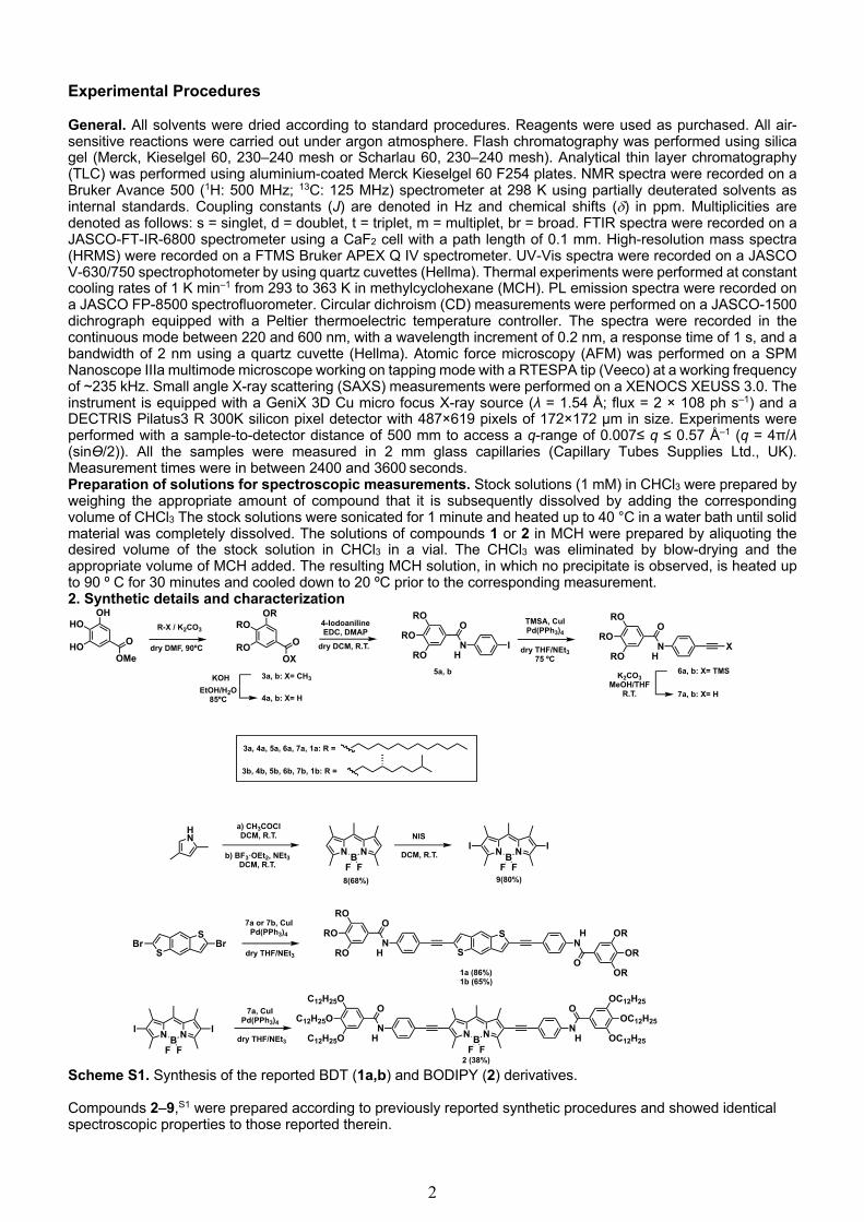
Scheme S1. Synthesis of the reported BDT (1a,b) and BODIPY (2) derivatives. Compounds 2‒9,S1 were prepared according to previously reported synthetic procedures and showed identical spectroscopic properties to those reported therein.

OHHO

HO O

OMe

ORRO

RO O

OX

3a, b: X= CH3

4a, b: X= H

S

SBr Br

S

SN

H

O

NH

O

RO

RO

RO

OR

OR

OR

N B NFF

I I N B NFF

NH

O

NH

OC12H25O

C12H25O

C12H25O

OC12H25

OC12H25

OC12H25

R-X / K2CO3

dry DMF, 90ºC

EtOH/H2O85ºC

K2CO3MeOH/THF

R.T.

7a or 7b, CuIPd(PPh3)4

dry THF/NEt3

dry THF/NEt3

RO

RO

RO

O

NH

Idry DCM, R.T.

5a, b

4-IodoanilineEDC, DMAP

KOH

RO

RO

RO

O

NH

X

6a, b: X= TMS

7a, b: X= H

1a (86%)1b (65%)

7a, CuIPd(PPh3)4

2 (38%)

HN

dry THF/NEt375 ºC

TMSA, CuIPd(PPh3)4

a) CH3COClDCM, R.T.

b) BF3·OEt2, NEt3DCM, R.T.

N B NFF

8(68%)

NIS

DCM, R.T. N B NFF

I I

9(80%)

3a, 4a, 5a, 6a, 7a, 1a: R =

3b, 4b, 5b, 6b, 7b, 1b: R =

3

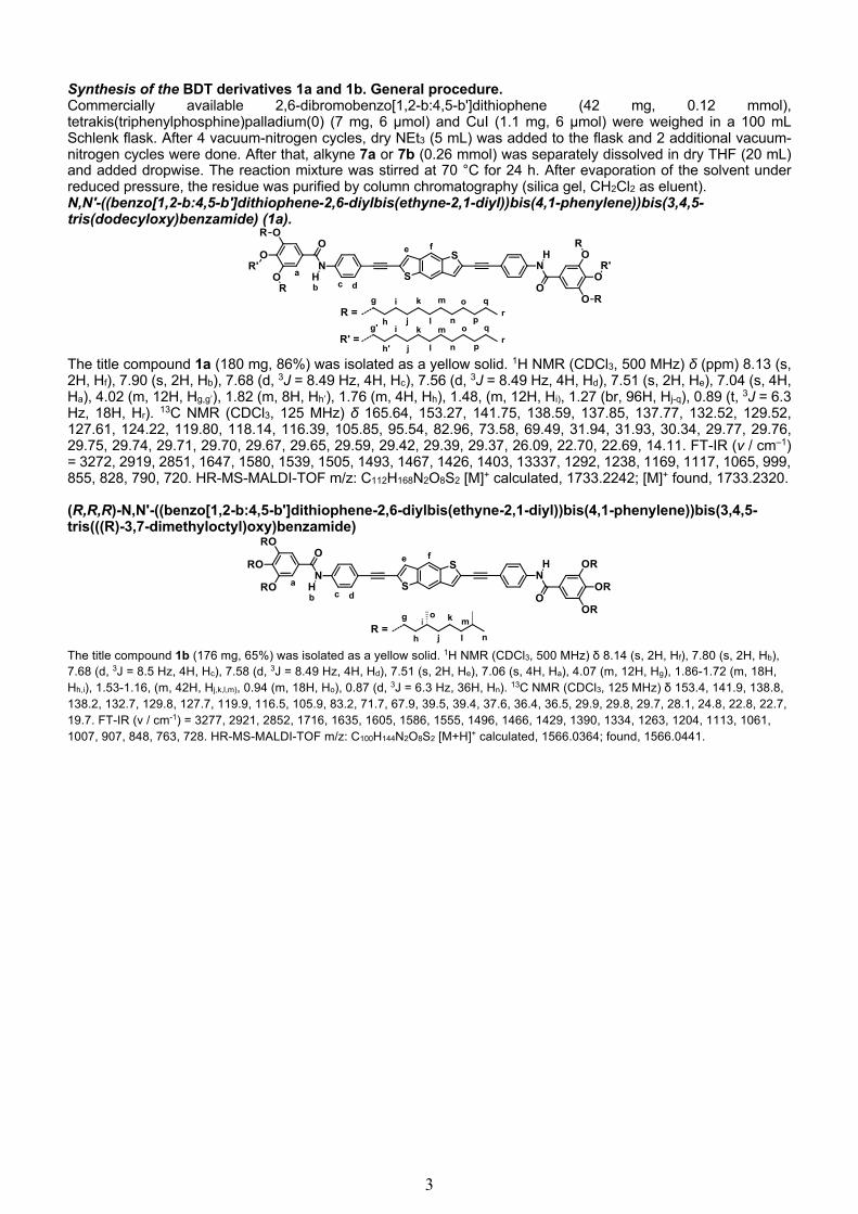
Synthesis of the BDT derivatives 1a and 1b. General procedure. Commercially available 2,6-dibromobenzo[1,2-b:4,5-b']dithiophene (42 mg, 0.12 mmol), tetrakis(triphenylphosphine)palladium(0) (7 mg, 6 μmol) and CuI (1.1 mg, 6 μmol) were weighed in a 100 mL Schlenk flask. After 4 vacuum-nitrogen cycles, dry NEt3 (5 mL) was added to the flask and 2 additional vacuum-nitrogen cycles were done. After that, alkyne 7a or 7b (0.26 mmol) was separately dissolved in dry THF (20 mL) and added dropwise. The reaction mixture was stirred at 70 °C for 24 h. After evaporation of the solvent under reduced pressure, the residue was purified by column chromatography (silica gel, CH2Cl2 as eluent). N,N'-((benzo[1,2-b:4,5-b']dithiophene-2,6-diylbis(ethyne-2,1-diyl))bis(4,1-phenylene))bis(3,4,5-tris(dodecyloxy)benzamide) (1a).

The title compound 1a (180 mg, 86%) was isolated as a yellow solid. 1H NMR (CDCl3, 500 MHz) δ (ppm) 8.13 (s, 2H, Hf), 7.90 (s, 2H, Hb), 7.68 (d, 3J = 8.49 Hz, 4H, Hc), 7.56 (d, 3J = 8.49 Hz, 4H, Hd), 7.51 (s, 2H, He), 7.04 (s, 4H, Ha), 4.02 (m, 12H, Hg,g’), 1.82 (m, 8H, Hh’), 1.76 (m, 4H, Hh), 1.48, (m, 12H, Hi), 1.27 (br, 96H, Hj-q), 0.89 (t, 3J = 6.3 Hz, 18H, Hr). 13C NMR (CDCl3, 125 MHz) δ 165.64, 153.27, 141.75, 138.59, 137.85, 137.77, 132.52, 129.52, 127.61, 124.22, 119.80, 118.14, 116.39, 105.85, 95.54, 82.96, 73.58, 69.49, 31.94, 31.93, 30.34, 29.77, 29.76, 29.75, 29.74, 29.71, 29.70, 29.67, 29.65, 29.59, 29.42, 29.39, 29.37, 26.09, 22.70, 22.69, 14.11. FT-IR (ν / cm‒1) = 3272, 2919, 2851, 1647, 1580, 1539, 1505, 1493, 1467, 1426, 1403, 13337, 1292, 1238, 1169, 1117, 1065, 999, 855, 828, 790, 720. HR-MS-MALDI-TOF m/z: C112H168N2O8S2 [M]+ calculated, 1733.2242; [M]+ found, 1733.2320. (R,R,R)-N,N'-((benzo[1,2-b:4,5-b']dithiophene-2,6-diylbis(ethyne-2,1-diyl))bis(4,1-phenylene))bis(3,4,5-tris(((R)-3,7-dimethyloctyl)oxy)benzamide)

The title compound 1b (176 mg, 65%) was isolated as a yellow solid. 1H NMR (CDCl3, 500 MHz) δ 8.14 (s, 2H, Hf), 7.80 (s, 2H, Hb), 7.68 (d, 3J = 8.5 Hz, 4H, Hc), 7.58 (d, 3J = 8.49 Hz, 4H, Hd), 7.51 (s, 2H, He), 7.06 (s, 4H, Ha), 4.07 (m, 12H, Hg), 1.86-1.72 (m, 18H, Hh,i), 1.53-1.16, (m, 42H, Hj,k,l,m), 0.94 (m, 18H, Ho), 0.87 (d, 3J = 6.3 Hz, 36H, Hn). 13C NMR (CDCl3, 125 MHz) δ 153.4, 141.9, 138.8, 138.2, 132.7, 129.8, 127.7, 119.9, 116.5, 105.9, 83.2, 71.7, 67.9, 39.5, 39.4, 37.6, 36.4, 36.5, 29.9, 29.8, 29.7, 28.1, 24.8, 22.8, 22.7, 19.7. FT-IR (ν / cm-1) = 3277, 2921, 2852, 1716, 1635, 1605, 1586, 1555, 1496, 1466, 1429, 1390, 1334, 1263, 1204, 1113, 1061, 1007, 907, 848, 763, 728. HR-MS-MALDI-TOF m/z: C100H144N2O8S2 [M+H]+ calculated, 1566.0364; found, 1566.0441.

4

3. Collection of spectra

1H NMR (CDCl3, 500 MHz, 298 K) of compound 1a

13C NMR (CDCl3, 125 MHz, 298 K) of compound 1a

5

1H, 13C-HMQC spectrum (CDCl3, 298 K) of compound 1a

1H NMR (CDCl3, 500 MHz, 298 K) of compound 1b

6

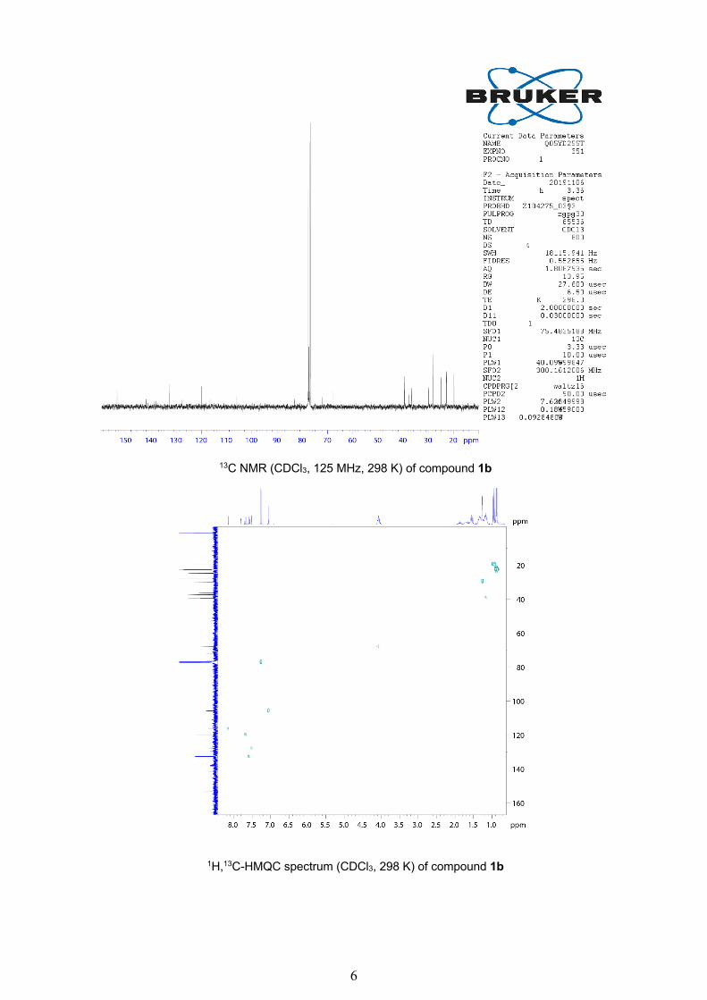
13C NMR (CDCl3, 125 MHz, 298 K) of compound 1b

1H,13C-HMQC spectrum (CDCl3, 298 K) of compound 1b

7

4. Supplementary Figures and Tables

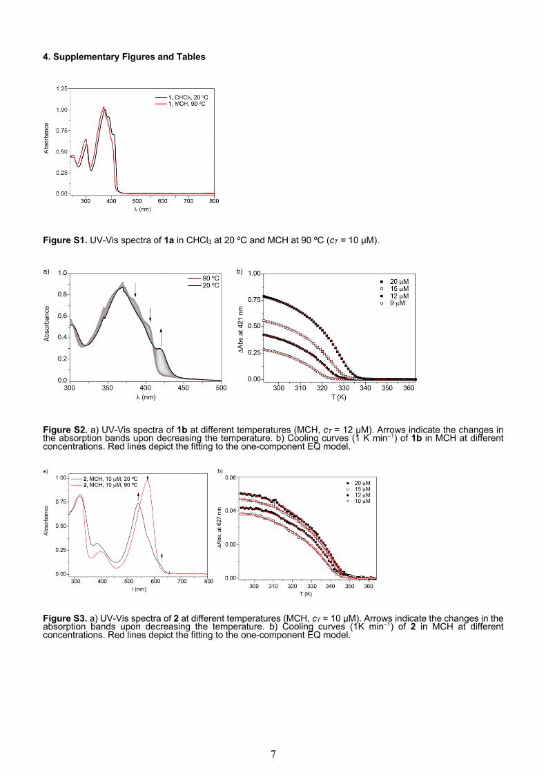
Figure S1. UV-Vis spectra of 1a in CHCl3 at 20 ºC and MCH at 90 ºC (cT = 10 µM).

Figure S2. a) UV-Vis spectra of 1b at different temperatures (MCH, cT = 12 µM). Arrows indicate the changes in the absorption bands upon decreasing the temperature. b) Cooling curves (1 K min‒1) of 1b in MCH at different concentrations. Red lines depict the fitting to the one-component EQ model.

Figure S3. a) UV-Vis spectra of 2 at different temperatures (MCH, cT = 10 µM). Arrows indicate the changes in the absorption bands upon decreasing the temperature. b) Cooling curves (1K min‒1) of 2 in MCH at different concentrations. Red lines depict the fitting to the one-component EQ model.

8

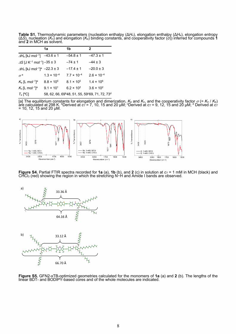
Table S1. Thermodynamic parameters (nucleation enthalpy (ΔHn), elongation enthalpy (ΔHe), elongation entropy (ΔS), nucleation (Kn) and elongation (Ke) binding constants, and cooperativity factor (σ)) inferred for compounds 1 and 2 in MCH as solvent.

1a 1b 2

DHe [kJ mol‒1] –43.6 ± 1 –54.8 ± 1 –47.3 ± 1

DS [J K‒1 mol‒1] –35 ± 3 –74 ± 1 –44 ± 3

DHn [kJ mol‒1]a –22.3 ± 3 –17.4 ± 1 –20.0 ± 3

s a 1.3 × 10–4 7.7 × 10–4 2.6 × 10–4

Ke [L mol‒1]a 8.8 × 105 8.1 × 105 1.4 × 106

Kn [L mol‒1]a 9.1 × 101 6.2 × 102 3.6 × 102 Te [ºC] 58, 62, 66, 69b 48, 51, 55, 59c 69, 71, 72, 73d

[a] The equilibrium constants for elongation and dimerization, Ke and Kn, and the cooperativity factor s (= Kn / Ke) are calculated at 298 K. bDerived at cT = 7, 10, 15 and 20 µM; cDerived at cT = 9, 12, 15 and 20 µM; d Derived at cT = 10, 12, 15 and 20 µM.

Figure S4. Partial FTIR spectra recorded for 1a (a), 1b (b), and 2 (c) in solution at cT = 1 mM in MCH (black) and CHCl3 (red) showing the region in which the stretching N−H and Amide I bands are observed.

Figure S5. GFN2-xTB-optimized geometries calculated for the monomers of 1a (a) and 2 (b). The lengths of the linear BDT- and BODIPY-based cores and of the whole molecules are indicated.

9

Figure S6. Height AFM images (a-c) and height profiles along the green line (d-f) of 1a (a, d), 1b (b, e), and 2 (c, f). Experimental conditions for AFM imaging: mica as surface; MCH, cT = 25 µM, spin coating.

Figure S7. Experimental SAXS profiles (black symbols) for (a) 1a (2.5 mM), (b) 1b (2.5 mM), and (c) 2 (2.6 mM) in MCH, and the corresponding fitting curves (red lines) to the elliptical cylinder model.

10

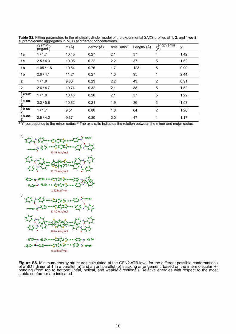
Table S2. Fitting parameters to the elliptical cylinder model of the experimental SAXS profiles of 1, 2, and 1-co-2 supramolecular aggregates in MCH at different concentrations.

cT (mM) / (mg/mL) ra (Å) r error (Å) Axis Ratiob Length/ (Å) Length error

(Å) χ²

1a 1 / 1.7 10.45 0.27 2.1 37 4 1.42

1a 2.5 / 4.3 10.05 0.22 2.2 37 5 1.52

1b 1.05 / 1.6 10.54 0.75 1.7 123 5 0.90

1b 2.6 / 4.1 11.21 0.27 1.6 95 1 2.44

2 1 / 1.8 9.80 0.23 2.2 43 2 0.91

2 2.6 / 4.7 10.74 0.32 2.1 38 5 1.52 1a-co-2 1 / 1.8 10.43 0.28 2.1 37 5 1.22 1a-co-2 3.3 / 5.8 10.82 0.21 1.9 36 3 1.53 1b-co-2 1 / 1.7 9.51 0.80 1.8 64 2 1.26 1b-co-2 2.5 / 4.2 9.37 0.30 2.0 47 1 1.17

a “r” corresponds to the minor radius. b The axis ratio indicates the relation between the minor and major radius.

Figure S8. Minimum-energy structures calculated at the GFN2-xTB level for the different possible conformations of a BDT dimer of 1 in a parallel (a) and an antiparallel (b) stacking arrangement, based on the intermolecular H-bonding (from top to bottom: lineal, helical, and weakly directional). Relative energies with respect to the most stable conformer are indicated.

11

Table S3. Relative energies calculated at the B3LYP-D3/6-31G(d,p) level of theory for the different possible conformations of the BDT dimer of 1 sketched in Figure S8.

Conformer Erel (kcal mol‒1)

lineal parallel 13.40 helical parallel 12.09 weakly directional parallel 1.04 lineal antiparallel 12.73 helical antiparallel 11.40 weakly directional antiparallel 0.00

Figure S9. Minimum-energy structures calculated at the GFN2-xTB level for the parallel (top) and antiparallel (bottom) stacking arrangements in the BODIPY dimer of 2. Relative energies with respect to the most stable conformer are indicated.

Figure S10. Minimum-energy structures calculated at the GFN2-xTB level for a decamer stacking of BDT 1 (a) and BODIPY 2 (b) without peripheral aliphatic chains. Relevant intermolecular mean distances (in Å) calculated for the decamer are indicated in (b).

12

Figure S11. Evolution of the binding energy per interacting pair as a function of the number of monomers (n) calculated at the GFN2-xTB level for slipped (a) and helical (b) supramolecular assemblies of BDT 1 (without peripheral aliphatic chains) with a parallel stacking of the core. Transparent red lines are drawn to guide the eye.

Figure S12. Evolution of the binding energy per interacting pair as a function of the number of monomers (n) calculated at the GFN2-xTB level for slipped (a) and helical (b) supramolecular assemblies of BDT 1 (without peripheral aliphatic chains) with an antiparallel stacking of the core. Transparent red lines are drawn to guide the eye.

Figure S13. Evolution of the binding energy per interacting pair as a function of the number of monomers (n) calculated at the GFN2-xTB level for slipped (a) and helical (b) supramolecular assemblies of BDT 1 (with peripheral aliphatic chains) with a parallel stacking of the core. Transparent red lines are drawn to guide the eye.

13

Figure S14. Evolution of the binding energy per interacting pair as a function of the number of monomers (n) calculated at the GFN2-xTB level for slipped (a) and helical (b) supramolecular assemblies of BDT 1 (with peripheral aliphatic chains) with an antiparallel stacking of the core. Transparent red lines are drawn to guide the eye.

Figure S15. Evolution of the binding energy per interacting pair as a function of the number of monomers (n) calculated at the GFN2-xTB level for the most stable arrangement of BODIPY 2 without (a) and with (b) peripheral aliphatic chains. The orange point in b) corresponds to a central-distorted 20-mer (see Figure S15b). Transparent red lines are drawn to guide the eye.

14

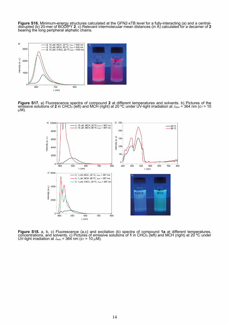
Figure S16. Minimum-energy structures calculated at the GFN2-xTB level for a fully-interacting (a) and a central-disrupted (b) 20-mer of BODIPY 2. c) Relevant intermolecular mean distances (in Å) calculated for a decamer of 2 bearing the long peripheral aliphatic chains.

Figure S17. a) Fluorescence spectra of compound 2 at different temperatures and solvents. b) Pictures of the emissive solutions of 2 in CHCl3 (left) and MCH (right) at 20 ºC under UV-light irradiation at lexc = 364 nm (cT = 10 µM).

Figure S18. a, b, c) Fluorescence (a,c) and excitation (b) spectra of compound 1a at different temperatures, concentrations, and solvents. c) Pictures of emissive solutions of 1 in CHCl3 (left) and MCH (right) at 20 ºC under UV-light irradiation at lexc = 364 nm (cT = 10 µM).

15

Figure S19. UV-Vis spectra of an equimolar mixture of 1a and 2 at different experimental conditions of temperature and time using MCH as solvent (cT = 10 µM).

Figure S20. UV-Vis (a) and emission (b) spectra of mixtures of 1a and 2 at different ratios in MCH at 20 ºC (cT = 20 µM; λexc = 367 nm). Arrows indicate the changes in the absorption and emission bands upon increasing the amount of BODIPY 2.

Figure S21. Plot of the variation of the absorbance at l = 595 nm versus temperature cooling at 1 K min‒1 for 1a-co-2. Red curves correspond to the global fitting to the EQ model to guide the eye.

16

Figure S22. (a) CD spectrum of 1b in MCH. (b) Plot of the variation of the dichroic response at l = 595 nm in mixtures of 1b and 2 upon increasing the amount of added 2 (MCH, cT = 10 µM, 20 ºC). The red line in panel (b) corresponds to a Boltzamn fit to guide the eye.

Figure S23. SAXS data and fitting for 1a-co-2 (a, b) and 1b-co-2 (c, d) at 1 mM (a, c), 3.3 mM (b) and 2.5 mM (d) in MCH. The red lines depict the fitting to the elliptical cylinder mode.

17

Figure S24. Height AFM image (a) and height profile along the green line (b) of 1a-co-2. Experimental conditions for AFM imaging: mica as surface; MCH, cT = 25 µM, spin coating.

18

5. SAXS measurements For compounds 1a, 1b, and 2, the solid compound was dissolved in the appropriate amount of MCH (cT = 1 or 2.5 mM), heated to 90° for 2 minutes, and then allowed to cool and stabilize at room temperature for 24 h prior to the measurements. The samples of the co-assembled species (1a-co-2 and 1b-co-2) were prepared by mixing, at 1:1 ratio, CHCl3 solutions of 1a or 1b and 2 (cT = 1 mM) and then evaporating the solvent under argon flow. The resulting solid was re-dissolved in the appropriate amount of MCH and the sample was allowed to stabilize for 24 h prior to the measurements. Background subtraction (against the solvent) was carried out using the XSACT software (Xenocs). The subtracted curves were fitted to customized models using the software SASView. The curves were fitted to distinct models and the best fittings (χ²) for the SAXS curves of the 1, 2, and 1-co-2 supramolecular aggregates were obtained using the elliptical cylinder model (Table S2). 5. Theoretical calculations Theoretical calculations were performed by means of the xTB program package.S2 Full geometry optimizations were carried out at the cost-effective semiempirical GFN2-xTB level of theory, which uses a minimal valence basis set centred on atoms (STO-mG), and includes the latest density-dependent D4 dispersion correction.S3 Figures S5 and S8-S16 show the optimized geometries computed for monomers and for aggregates of increasing size (from the dimer to the 30-mer). The binding energy per interacting pair ( ) was calculated as:

where 𝐸!"#$!%&' is the energy for a specific oligomer, 𝐸%!(!%&' is the energy for the minimum-energy geometry of the corresponding monomer, and n is the number of monomeric units in the oligomer. Figures S11-S14 and Figure 5b,c in the main text show the evalution of with the size of the oligomer. Central-disrupted oligomers were built up by joining two optimized decamers, and then fully optimizing at the GFN2-xTB level (Figure S16b and Figure 6b). Solvent effects were included to assess dimer stability of BDT 1 by means of the generalized Born (GB) model with surface area (SA) contributions (termed GBSA approach). The relative energies calculated at the GFN2-xTB+GBSA level for the helical stacking arrangement with respect to the most stable cofacial, slightly long-axis slipped, antiparallel conformer in a BDT dimer of 1 were calculated to be 10.67, 5.14, 4.62, and 4.38 kcal mol‒1 in vacuum, n-hexane, chloroform, and toluene, respectively, thus confirming the higher energy of the helical dimer. Density functional theory calculations were also performed on the different conformations of the dimeric species of BDT 1 through the Gaussian-16.A03 suite of programs.S4 Geometry optimizations and single-point energy calculations were carried out by means of the popular hybrid B3LYP functionalS5 and the double-zeta Pople’s 6-31G(d,p) basis set, and including the Grimme’s D3 dispersion correction.S6,S7 Relative energies are summarized in Table S2. Geometry representations and analyses were done by means of the Chemcraft 1.7 software.S8

References

[S1] (a) A. Rödle, B. Ritschel, C. Mück-Lichtenfeld, V. Stepanenko, G. Fernández, Chem. Eur. J. 2016, 22, 15772–15777; (b) F. Wang, M. A. J. Gillissen, P. J. M. Stals, A. R. A. Palmans, E. W. Meijer, Chem. Eur. J. 2012, 18, 11761 – 11770

[S2] C. Bannwarth, E. Caldeweyher, S. Ehlert, A. Hansen, P. Pracht, J. Seibert, S. Spicher, S. Grimme, WIREs Comput. Mol. Sci., 2020, 11, e01493.

[S3] C. Bannwarth, S. Ehlert, S. Grimme, J. Chem. Theory Comput. 2019, 15, 1652–1671. [S4] Gaussian 16, Revision A.03, M. J. Frisch, G. W. Trucks, H. B. Schlegel, G. E. Scuseria, M. A. Robb, J. R. Cheeseman, G.

Scalmani, V. Barone, G. A. Petersson, H. Nakatsuji, X. Li, M. Caricato, A. V. Marenich, J. Bloino, B. G. Janesko, R. Gomperts, B. Mennucci, H. P. Hratchian, J. V. Ortiz, A. F. Izmaylov, J. L. Sonnenberg, D. Williams-Young, F. Ding, F. Lipparini, F. Egidi, J. Goings, B. Peng, A. Petrone, T. Henderson, D. Ranasinghe, V. G. Zakrzewski, J. Gao, N. Rega, G. Zheng, W. Liang, M. Hada, M. Ehara, K. Toyota, R. Fukuda, J. Hasegawa, M. Ishida, T. Nakajima, Y. Honda, O. Kitao, H. Nakai, T. Vreven, K. Throssell, J. A. Montgomery, Jr., J. E. Peralta, F. Ogliaro, M. J. Bearpark, J. J. Heyd, E. N. Brothers, K. N. Kudin, V. N. Staroverov, T. A. Keith, R. Kobayashi, J. Normand, K. Raghavachari, A. P. Rendell, J. C. Burant, S. S. Iyengar, J. Tomasi, M. Cossi, J. M. Millam, M. Klene, C. Adamo, R. Cammi, J. W. Ochterski, R. L. Martin, K. Morokuma, O. Farkas, J. B. Foresman, and D. J. Fox, Gaussian, Inc., Wallingford CT, 2016.

[S5] A. D. Becke, J. Chem. Phys. 1993, 98, 5648–5652. [S6] V. A. Rassolov, M. A. Ratner, J. A.; Pople, P. C. Redfern, L. A. Curtiss, J. Comp. Chem. 2001, 22, 976–984. [S7] S. Grimme, S. Ehrlich, L. Goerigk, J. Comp. Chem. 2011, 32, 1456-1465. [S8] Chemcraft - graphical software for visualization of quantum chemistry computations. https://www.chemcraftprog.com.