1

revised version: JPET # 05004

Business cycles, heuristic expectation formation and contracyclical policies*

Frank H. Westerhoff

University of Osnabrück, Department of Economics

Rolandstraße 8, D-49069 Osnabrück, Germany

fwesterho@oec.uni-osnabrueck.de

Abstract

We develop a simple Keynesian-type business cycle model in which agents use simple

heuristics to predict national income. To be precise, the agents either form (destabilizing)

extrapolative expectations or (stabilizing) regressive expectations, a decision which depends

on the rules forecasting performance in the recent past. As it turns out, an unending

evolutionary competition between the rules may generate endogenous complex business

cycles. We also explore the effectiveness of some common governmental intervention

strategies. Our model suggests that policy makers may be able to stabilize output fluctuations,

yet due to system immanent nonlinearities this may prove to be quite difficult.

Keywords

agent-based computational economics, business cycles,

heuristic expectation formation, contracyclical policies, complex dynamics

JEL classification

E32, E12, D84

___________________ * Presented at the annual meeting of the Macroeconomic Research Committee of the German Economic Association in Bonn, June 2005. I thank the participants, especially Jürgen von Hagen, for encouraging discussions. I also thank two anonymous referees and an associate editor for many helpful comments and suggestions.

2

1 Introduction

Short-run output variations are a world-wide phenomenon, basically all modern industrial

economies regularly experience significant swings in economic activity. Alternating periods

of expansion and contraction are naturally welfare-decreasing. Every recession in which

workers become involuntarily unemployed is associated with an income loss that cannot be

regained. Booms and recessions may have an exogenous trigger. However, complex output

movements may also arise endogenously due to nonlinearities (for excellent surveys see, e.g.,

Gandolfo 1985, Puu 1989, Medio 1992, Day and Chen 1993, Day 1999 or Rosser 2000).

Especially in the latter case, policy makers may want to stabilize the economy. But as

demonstrated by Baumol (1961), the variability of national income may increase if

intervention mechanisms are ill-designed. A thorough understanding of the causes of business

cycles thus seems to be quite important.

In this paper, we develop a business cycle model to analyze the role of expectation

formation for output fluctuations and to explore the usefulness of common contracyclical

intervention rules. Our starting point is that people are boundedly rational in the sense of

Simon (1955). Although agents lack the knowledge and computational capabilities to

determine optimal actions, they strive to do the right thing. As argued by Kahneman, Slovic

and Tversky (1986), people rely on a limited number of heuristic principles which reduce the

complex tasks of assessing probabilities and predicting values to simpler judgmental

operations. These heuristics face a natural selection pressure, i.e. only well-performing rules

survive. With respect to expectation formation, two popular types of heuristics exist.

Extrapolative expectations simply assume a continuation of the current trend and are thus

likely to be destabilizing. Regressive expectations are often regarded as a stabilizing force

since they add a negative feedback to the dynamics. Note that regressive expectations are

relatively sophisticated and thus may be more costly.

3

Guided by these empirical regularities, we develop a business cycle model in which

agents form simple (cheap) extrapolative or sophisticated (costly) regressive expectations to

predict their income. Moreover, the agents do not stick to a certain rule but compare their

relative fitness and tend to select the better one. Clearly, agents prefer heuristics which have

produced low squared prediction errors in the recent past. To make matters as simple as

possible, we use a Keynesian multiplier framework to describe the rest of the economy. A

central finding is that movements in national income may arise endogenously due to a

permanent competition between different heuristics. In periods in which extrapolative

expectations are dominating, the economy is unstable and strong cyclical output movements

occur. However, extrapolative predictors perform poorly at turning points. When regressive

expectations gain in popularity, a period of convergence sets in. Since prediction errors of

extrapolative expectations become low when output is relatively stable, at least some agents

return to this type of forecasting rule and thus output oscillations may increase again.

Policy makers frequently conduct contracyclical interventions to smooth business

cycles. But at least within our setup, this proves to be rather difficult. Both trend-adjusting

and level-adjusting strategies have, in principle, the potential to reduce the amplitude of

business fluctuations. However, success and failure of the interventions depend critically on

how the rules are executed. Already tiny mistakes in the strength of the interventions may

make a huge difference, turning a stable environment into an unstable one.

We continue as follows. In section 2, we first develop a business cycle model in which

agents follow heterogeneous expectation formation rules. In section 3, we discuss the

workings of the model. In section 4, we study the effectiveness of a few common

contracyclical intervention policies. In section 5, we explore several routes to business cycles.

The last section concludes the paper and points out some interesting avenues for future

research.

4

2 A simple business cycle model

In order to explore the impact of heuristic expectation formation on business cycles, the

economy is modeled as simply as possible. For this reason, we express national income Y at

time step t as

ttt CIY += , (1)

where

II t = (2)

comprises all autonomous expenditures.1 Consumption is a function of national income. But

instead of postulating that consumption depends on the last period’s output (according to the

so-called Robertson lag), we assume that the agents consume a constant fraction a of their

current expected income ][ tYE . Hence, we have

][ tt YaEC = . (3)

The consumption parameter a is restricted to 10 << a .

Note that for ][ tt YEYY == , (1)-(3) imply that

a

IY

−=

1, (4)

which corresponds to the well-known Keynesian multiplier solution. As in Baumol (1961),

we interpret the steady state Y as the near full employment output level.

As mentioned in the introduction, people frequently rely on simple heuristics such as

extrapolative and regressive forecasting rules to predict economic variables. The average

market expectation with respect to national income may therefore be defined as

1 Recent extensions of Samuelson’s (1939) multiplier-accelerator model include, for instance, Sushko, Puu and

Gardini (2003), Puu, Gardini and Sushko (2005) and Westerhoff (2005). Incorporating an investment function

makes, of course, the analysis more realistic, yet also more intricate. In order to highlight the role of expectation

formation for the emergence of output fluctuations, we treat investment as exogenously given and constant.

5

][][][ trr

ttee

tt YEWYEWYE += . (5)

The relative weight of extrapolative expectations ][ te YE is denoted by e

tW and the relative

weight of regressive expectations ][ tr YE is represented by r

tW with 1=+ rt

et WW .

When the agents compute their expected income for period t, they possess information

up to period t-1. Extrapolative expectations may then be formalized as

)(][ 211 −−− −+= tttte YYbYYE , (6)

where 0>b indicates how strongly the agents extrapolate past output changes into the future.

Regressive expectations may be written as

)(][ 11 −− −+= tttr YYcYYE . (7)

Accordingly, the agents expect the gap between the near full employment output level Y and

the observed output level 1−tY to be reduced by a factor 10 << c .

Now we turn to the crucial part of the model. The agents do not stick to a certain

predictor but compare their relative performance. Here, we measure the fitness of the rules by

their squared prediction error. The agents consequently favor rules with low prediction errors.

To be precise, the attractiveness of extrapolative expectations is given as

211. )][( −− −−= tt

eet YYEA . (8)

While it is straightforward to extrapolate trends, computing regressive expectations is a more

sophisticated task. For instance, people have to estimate the near full employment output level

Y . For being able to do this, they first have to develop some general knowledge about how

the economy may work. The attractiveness of regressive expectations is thus modeled as

211. )][( −− −−−= tt

rrt YYEdA , (9)

6

where 0≥d captures the costs associated with applying the more sophisticated predictor.2

The relevance of the different forecasting rules depends on their relative fitness: The

higher the fitness of a predictor, the more agents will follow it.3 As in the discrete-choice

approach of Manski and McFadden (1981), the weights of the two predictors are given as

]exp[]exp[

]exp[rt

et

ete

thAhA

hAW

+= (10)

and

]exp[]exp[

]exp[rt

et

rtr

thAhA

hAW

+= . (11)

The parameter 0≥h may be regarded as the intensity of choice and measures how sensitive

the mass of agents is to selecting the most attractive predictor. Note that an increase in h may

be interpreted as an increase in the rationality of the agents. For 0=h , the agents do not

discriminate between the predictors and thus they split evenly between them. But if h goes to

infinity, all agents select the predictor with the highest fitness.

Combining (1)-(11) reveals that

),,( 321 −−−= tttt YYYfY , (12)

i.e. the recurrence relation which determines national income is a three-dimensional nonlinear

difference equation.4 Due to the functional form of (12), we continue with numerical analysis.

One advantage of our simple setup is that it should be quite easy to replicate the simulations.

2 In section 5, we will see that this assumption is not crucial, complex dynamics may also arise for 0=d .

However, assuming that the formation of regressive expectations is more costly than the formation of

extrapolative expectations seems to be more natural and thus we take this aspect into account. 3 The modeling of predictor choice is inspired by the work of Brock and Hommes (1997, 1998). While the

former contribution is concerned with the expectation formation of heterogeneous producers within a cobweb

framework, the latter focuses on financial market dynamics. An excellent introduction into agent-based

computational models is Judge and Tesfatsion (2006).

4 It is easy to calculate that the unique steady state of (12) is given by the near full employment output level Y .

7

3 The emergence of business cycles: An example

We assume the following basic parameter setting for our simulations analysis:

9.0=a , 4.1=b , 15.0=c , 2.1=d , 1=h .

In addition, autonomous expenditures are fixed at 1000=I . Since the “multiplier” is 10, the

near full employment output level is 10000=Y . Moreover the initial conditions of our three-

dimensional system are given as 100001 =Y , 100002 =Y and 100013 =Y (i.e. we slightly

disturb the steady state in period 3=t ).5 Note that if national income is for at least two

consecutive periods equal to Y , then the agents expect output to be stable and thus it is. But

due to the heuristic expectation formation process, output is – at least within our setup – not

necessarily stable.

Figure 1 shows a typical simulation run. The top panel presents the evolution of output

for 500 observations (after omitting a longer transient period). Although the dynamics is

entirely deterministic, we observe the emergence of expansions, followed by recessions. The

sequence of booms and slumps is recurrent, but not periodic. Both the duration of business

cycles and their amplitude vary. In a stylized way, the simulated output dynamics resembles

actual fluctuations in economic activity (Stock and Watson 1999).

= = = = = Figure 1 goes about here = = = = =

What drives the dynamics? The bottom panel depicts the weight of the extrapolative

predictor. Note that in most cases either all agents form regressive or extrapolative

expectations. Suppose that all agents use the regressive predictor, i.e. 0=etW and 1=r

tW .

Then the law of motion of national income is given as

1)( −−++= tt YacaYacIY , (13)

5 The dynamics discussed in this section does not depend on our choice of initial conditions. Section 5, however,

demonstrates that initial conditions may become critical for other parameter combinations.

8

which is a one-dimensional linear difference equation. The steady state of (13) is equal to

)1/( aIY −= . Moreover, monotonic convergence towards the steady state sets in if

1)(0 <−< aca . (14)

Since 10 << a and 10 << c , (14) is always true. Hence, if all agents use the regressive

forecasting rule, national income monotonically converges towards its steady state level.

Let us now turn to the case in which all agents prefer the extrapolative heuristic, i.e.

1=etW and 0=r

tW . Then we obtain the following second-dimensional linear difference

equation

21)( −− −++= ttt abYYabaIY . (15)

Obviously, the steady state is given as )1/( aIY −= . Rewriting Schur’s stability conditions6

delivers

1<a (16)

and

ba /1< . (17)

Furthermore, we can compute that (15) generates cycles if

2)1/(4 bba +< . (18)

Since 9.0=a and 4.1=b , our model produces unstable cyclical motion when all agents rely

on extrapolative expectations.

But as is visible in figure 1, output neither settles down on its fixed point nor does it

explode. Instead, we observe frequent, yet irregular regime shifts. For some time, regressive

expectations may appear superior. Then the economy behaves stably and output approaches

6 Remember that a second-dimensional linear difference equation YXaXaX ttt =++ −− 2211 is stable if (1)

01 21 >++ aa , (2) 01 21 >+− aa and (3) 01 2 >− a . The conditions for cycles is 221 4aa < .

9

its near full employment level. But when output is close to Y , the prediction errors of both

types of predictors become small. Since regressive expectation formation is relatively costly,

the extrapolative predictor appears to be more attractive. As a result, agents now trend-

extrapolate output changes and increasing output oscillations emerge. At some point in time,

however, extrapolative expectations produce quite strong prediction errors (especially at

turning points, i.e. local maxima and minima). Although regressive expectation formation is

costly, it eventually becomes advantageously again. Then a period of convergence sets in

until the pattern repeats itself, yet in a complex way. Clearly, it is the endogenous adaptation

process of the agents that creates business cycles.

4 Some policy experiments

So far we have seen that the agent’s expectation formation process may lead to an ebb and

flow of economic activity. Note that if the dynamics is endogenous, then policy makers may

have a chance to stabilize economic activity. Following Baumol (1961), we discuss two

common intervention measures. The first policy aims at adjusting income levels. Suppose the

government always decides to compensate for the difference between actual output and its

near full employment level. Such a level-adjusting policy may be formalized as

)( 1−−= tLL

t YYgG , (19)

where 0>Lg is the policy maker’s control parameter. As long as output is below Y , the

government increases its spending (and vice versa).7 The aggregated intervention volume

�=

=T

t

LtGD

1

, (20)

7 The national income equation (1) now has on its right-hand side autonomous expenditures, consumption and government interventions. The system remains, of course, three dimensional.

10

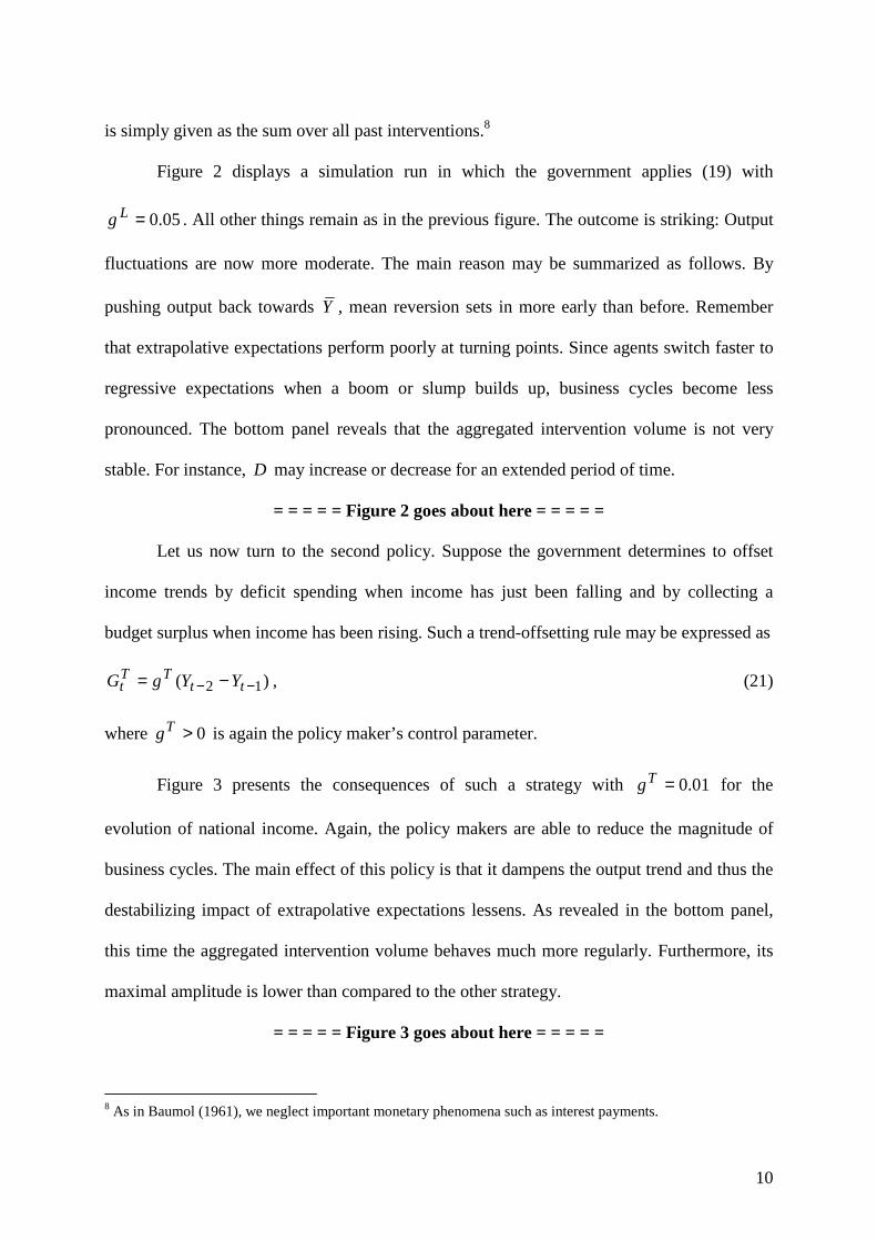
is simply given as the sum over all past interventions.8

Figure 2 displays a simulation run in which the government applies (19) with

05.0=Lg . All other things remain as in the previous figure. The outcome is striking: Output

fluctuations are now more moderate. The main reason may be summarized as follows. By

pushing output back towards Y , mean reversion sets in more early than before. Remember

that extrapolative expectations perform poorly at turning points. Since agents switch faster to

regressive expectations when a boom or slump builds up, business cycles become less

pronounced. The bottom panel reveals that the aggregated intervention volume is not very

stable. For instance, D may increase or decrease for an extended period of time.

= = = = = Figure 2 goes about here = = = = =

Let us now turn to the second policy. Suppose the government determines to offset

income trends by deficit spending when income has just been falling and by collecting a

budget surplus when income has been rising. Such a trend-offsetting rule may be expressed as

)( 12 −− −= ttTT

t YYgG , (21)

where 0>Tg is again the policy maker’s control parameter.

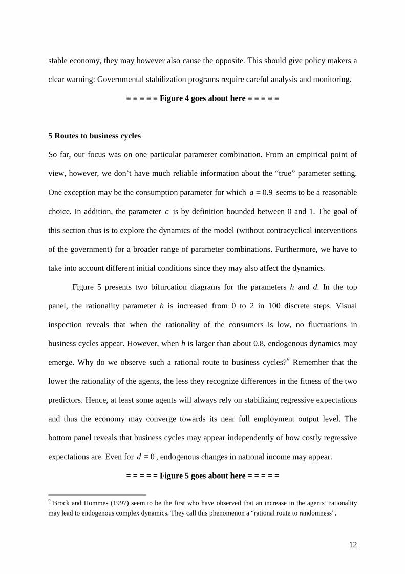
Figure 3 presents the consequences of such a strategy with 01.0=Tg for the

evolution of national income. Again, the policy makers are able to reduce the magnitude of

business cycles. The main effect of this policy is that it dampens the output trend and thus the

destabilizing impact of extrapolative expectations lessens. As revealed in the bottom panel,

this time the aggregated intervention volume behaves much more regularly. Furthermore, its

maximal amplitude is lower than compared to the other strategy.

= = = = = Figure 3 goes about here = = = = =

8 As in Baumol (1961), we neglect important monetary phenomena such as interest payments.

11

Overall, one may be tempted to argue that both intervention strategies are useful to

reduce output fluctuations. But is such an optimistic conclusion really justified? Already

Baumol (1961) remarked that plausible and reasonable contracyclical policies may turn out to

be a dangerous tool. In his linear (multiplier-accelerator) framework, trend-offsetting and

level-adjusting policies may, contrary to the economists intuition, aggravate fluctuations in

economic activity. Let us therefore explore what happens in our nonlinear model if the

government uses different control parameters.

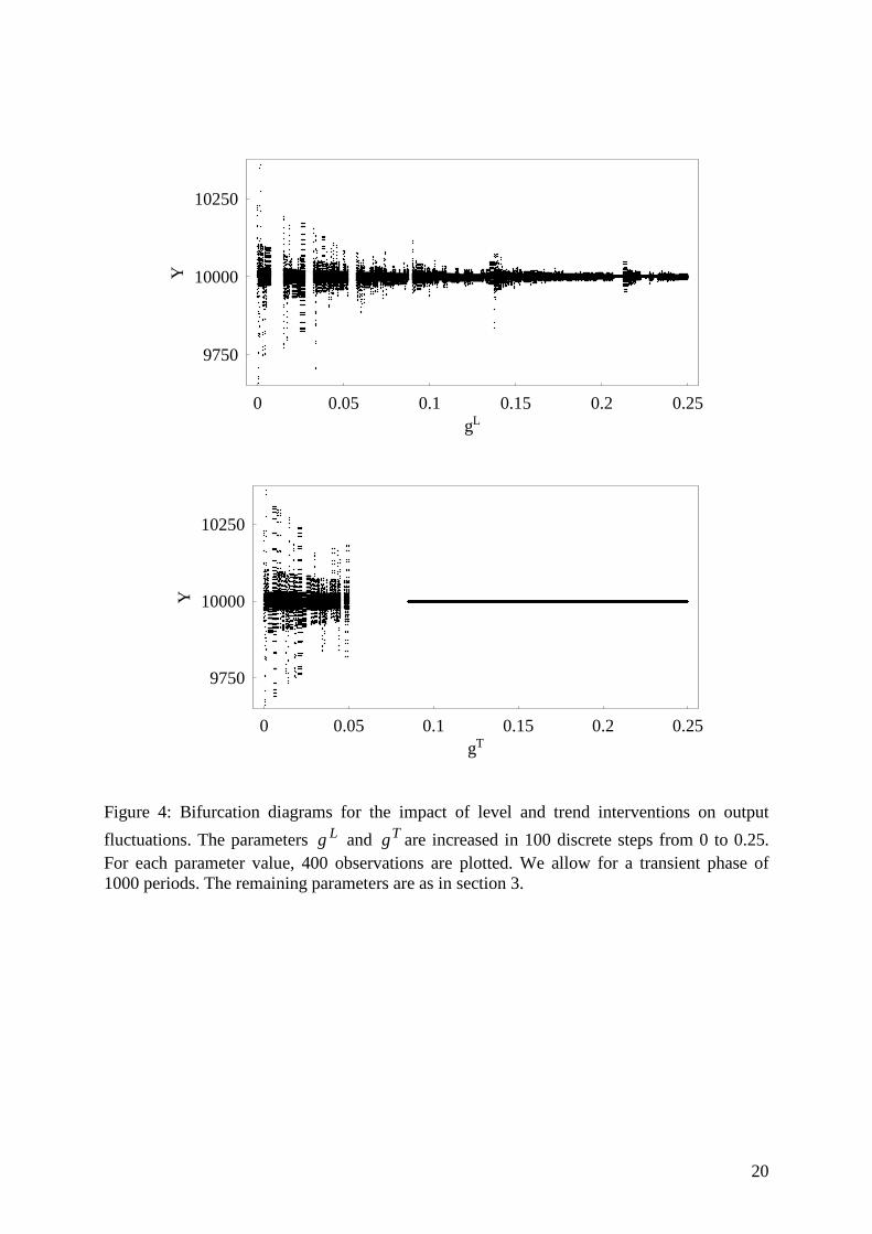
Figure 4 contains two bifurcation diagrams for the impact of level and trend

interventions on output fluctuations. The control parameters Lg (top panel) and Tg (bottom

panel) are increased in 100 discrete steps from 0 to 0.25. For each value of the control

parameter, 400 observations are plotted, after discarding a transient phase of 1000 periods.

The remaining parameters are as in section 3. Bifurcation diagrams are a powerful graphical

instrument, illustrating the dynamic behavior of a system for a wide range of the underlying

bifurcation parameters.

What are the results? Roughly speaking, the maximal amplitude tends to decrease as

the two bifurcation parameters increase. Unfortunately, there are some dramatic interruptions

of this process. Both types of intervention strategies may for some parameter values yield an

explosion of the system (these areas are represented by blanks in the bifurcation diagrams).

This is, for instance, the case for about 075.005.0 << Tg . Surprisingly, for

25.0075.0 << Tg the same strategy completely stabilizes output motion. Similar results are

observed for the other strategy. For, e.g., 23.0=Lg , the level-adjusting policy eliminates

fluctuations in economic activity, yet for, e.g., 055.0=Lg the same strategy triggers an

unstable orbit. To sum up, simple and well-intended intervention policies may lead to a more

12

stable economy, they may however also cause the opposite. This should give policy makers a

clear warning: Governmental stabilization programs require careful analysis and monitoring.

= = = = = Figure 4 goes about here = = = = =

5 Routes to business cycles

So far, our focus was on one particular parameter combination. From an empirical point of

view, however, we don’ t have much reliable information about the “ true” parameter setting.

One exception may be the consumption parameter for which 9.0=a seems to be a reasonable

choice. In addition, the parameter c is by definition bounded between 0 and 1. The goal of

this section thus is to explore the dynamics of the model (without contracyclical interventions

of the government) for a broader range of parameter combinations. Furthermore, we have to

take into account different initial conditions since they may also affect the dynamics.

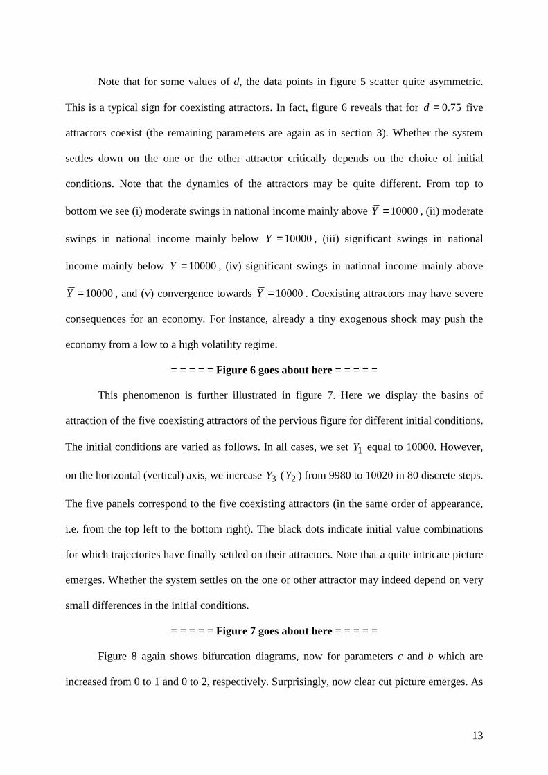
Figure 5 presents two bifurcation diagrams for the parameters h and d. In the top

panel, the rationality parameter h is increased from 0 to 2 in 100 discrete steps. Visual

inspection reveals that when the rationality of the consumers is low, no fluctuations in

business cycles appear. However, when h is larger than about 0.8, endogenous dynamics may

emerge. Why do we observe such a rational route to business cycles?9 Remember that the

lower the rationality of the agents, the less they recognize differences in the fitness of the two

predictors. Hence, at least some agents will always rely on stabilizing regressive expectations

and thus the economy may converge towards its near full employment output level. The

bottom panel reveals that business cycles may appear independently of how costly regressive

expectations are. Even for 0=d , endogenous changes in national income may appear.

= = = = = Figure 5 goes about here = = = = =

9 Brock and Hommes (1997) seem to be the first who have observed that an increase in the agents’ rationality

may lead to endogenous complex dynamics. They call this phenomenon a “rational route to randomness” .

13

Note that for some values of d, the data points in figure 5 scatter quite asymmetric.

This is a typical sign for coexisting attractors. In fact, figure 6 reveals that for 75.0=d five

attractors coexist (the remaining parameters are again as in section 3). Whether the system

settles down on the one or the other attractor critically depends on the choice of initial

conditions. Note that the dynamics of the attractors may be quite different. From top to

bottom we see (i) moderate swings in national income mainly above 10000=Y , (ii) moderate

swings in national income mainly below 10000=Y , (iii) significant swings in national

income mainly below 10000=Y , (iv) significant swings in national income mainly above

10000=Y , and (v) convergence towards 10000=Y . Coexisting attractors may have severe

consequences for an economy. For instance, already a tiny exogenous shock may push the

economy from a low to a high volatility regime.

= = = = = Figure 6 goes about here = = = = =

This phenomenon is further illustrated in figure 7. Here we display the basins of

attraction of the five coexisting attractors of the pervious figure for different initial conditions.

The initial conditions are varied as follows. In all cases, we set 1Y equal to 10000. However,

on the horizontal (vertical) axis, we increase 3Y ( 2Y ) from 9980 to 10020 in 80 discrete steps.

The five panels correspond to the five coexisting attractors (in the same order of appearance,

i.e. from the top left to the bottom right). The black dots indicate initial value combinations

for which trajectories have finally settled on their attractors. Note that a quite intricate picture

emerges. Whether the system settles on the one or other attractor may indeed depend on very

small differences in the initial conditions.

= = = = = Figure 7 goes about here = = = = =

Figure 8 again shows bifurcation diagrams, now for parameters c and b which are

increased from 0 to 1 and 0 to 2, respectively. Surprisingly, now clear cut picture emerges. As

14

is visible in the top panel, when c is too low or too high, the system is not stable and an

explosion may occur (these areas are represented by blanks in the bifurcation diagram). The

bottom panel shows that when b is low, the system may approach its steady state level.

However, when b increases, complex dynamics but also unstable trajectories may appear.

= = = = = Figure 8 goes about here = = = = =

Let us finally explore for which combinations of h versus d and c versus b the system

generates stable or unstable trajectories. The left panel of figure 9 shows the basin of

attraction for parameter h versus d which are both increased from 0 to 2 in 80 discrete steps

(the remaining parameters are as in section 3). The black dots then indicate parameter

combinations which do not trigger explosions. The right panel shows the same for the

parameters c and d which are increased from 0 to 1 and 0 to 2, respectively. Interestingly,

independently of parameters h and d, only none-explosive trajectories are observed. However,

this is not the case for parameters c and b. In particular, if b exceeds a certain threshold, the

evolution of national income may become unstable. Note that the pattern which emerges is

intricate, there also exists some islands of stability.

= = = = = Figure 9 goes about here = = = = =

6 Conclusions

Our aim is to study the impact of heuristic expectation formation on fluctuations in economic

activity when boundedly rational agents may select between competing predictors. Within our

model, agents have the choice between simple and cheap extrapolative and sophisticated, yet

costly regressive expectations. The agents prefer rules which possess a high fitness, i.e.

produce low squared prediction errors. Since competition between the predictors introduces a

nonlinearity, complex fluctuations in economic activity may emerge.

At least at first sight, this may give policy makers an opportunity to stabilize the

15

economy. And indeed, for certain specifications of the intervention strategies, output

variability declines. Unfortunately, life is more complicated, especially in a nonlinear world.

Common policies such as trend offsetting or level-adjusting interventions turn out to be a

mixed blessing. If the policy makers pick the wrong intervention strength – and here tiny

differences may already matter – output fluctuations are amplified. This again demonstrates

that it is important to understand the causes of business cycles.

Let us finally point out some avenues for future research. First, within our model,

agents who form regressive expectations are able to compute the near full employment output

level. Given their level of rationality, this may appear as a rather strong assumption. A

promising extension may be to consider the case in which boundedly rational agents seek to

learn this output level from current and past observations. Second, we ignore important

monetary phenomena. It would be interesting to see how private and governmental activity

may affect the interest rate and how this, in turn, may feed back on their behavior. We hope

that our paper will stimulate further work in this important research direction.

16

References

Baumol, W. (1961): Pitfalls in contracyclical policies: some tools and results. Review of

Economics and Statistics, 435, 21-26.

Brock, W. and Hommes. C. (1997): A rational route to randomness. Econometrica, 65, 1059-

1095.

Brock, W. and Hommes. C. (1998): Heterogeneous beliefs and routes to chaos in a simple

asset pricing model. Journal of Economic Dynamics and Control, 22, 1235-1274.

Day, R. and Chen, P. (1993): Nonlinear dynamics and evolutionary economics. Oxford

University Press: Oxford.

Day, R. (1999): Complex economic dynamics: an introduction to macroeconomic dynamics

(Volume 2). MIT Press: Cambridge.

Gandolfo, G. (1985): Economic dynamics: methods and models. North-Holland: Amsterdam.

Judd, K. and Tesfatsion, L. (2006): Handbook of computational economics (Volume 2):

Agent-based computational economics. North-Holland: Amsterdam.

Kahneman, D., Slovic, P. and Tversky, A. (1986): Judgment under uncertainty: heuristics and

biases. Cambridge University Press: Cambridge.

Manski, C. and McFadden, D. (1981): Structural analysis of discrete data with econometric

applications. MIT Press: Cambridge.

Medio, A. (1992): Chaotic dynamics. Cambridge University Press: Cambridge.

Puu, T. (1989): Nonlinear economic dynamics. Lecture notes in economics and mathematical

systems 336. Springer: Berlin.

Puu, T., Gardini, L. and Sushko, I. (2005): A multiplier-accelerator model with floor

determined by capital stock. Journal of Economic Behavior and Organization, 56, 331-348.

Rosser, J. B. (2000): From catastrophe to chaos: a general theory of economic discontinuities

(second edition). Kluwer Academic Publishers: Boston.

Samuelson, P. (1939): Interactions between the multiplier analysis and the principle of

acceleration. Review of Economics and Statistics, 21, 75-78.

Simon, H. (1955): A behavioral model of rational choice. Quarterly Journal of Economics, 9,

99-118.

Stock, J. and Watson, M. (1999): Business cycle fluctuations in U.S. macroeconomic time

series. In: Taylor, J. and Woodford, M. (eds): Handbook of macroeconomics. North-

Holland: Amsterdam, 3-64.

Sushko, I., Puu, T. and Gardini, L. (2003): The Hicksian floor-roof model for two regions

linked by interregional trade. Chaos, Solitons and Fractals, 18, 593-612.

Westerhoff, F. (2005): Samuelson’s multiplier-accelerator model revisited. Applied

Economics Letters, in press.

17

1 100 200 300 400 500time step

0.5

0

1

Wte

1 100 200 300 400 500time step

10000

10250

9750

Yt

Figure 1: The evolution of national income and the impact of the predictors for 500 observations. Parameter setting as in section 3.

18

1 100 200 300 400 500time step

-15

0

15

D

1 100 200 300 400 500time step

10000

10250

9750

Yt

Figure 2: The evolution of national income and accumulated governmental interventions for

500 observations. Parameter setting as in section 3, but 05.0=Lg .

19

1 100 200 300 400 500time step

-0.5

0

0.5

D

1 100 200 300 400 500time step

10000

10250

9750

Yt

Figure 3: The evolution of national income and accumulated governmental interventions for

500 observations. Parameter setting as in section 3, but 01.0=Tg .

20

0 0.05 0.1 0.15 0.2 0.25gT

10000

10250

9750

Y

0 0.05 0.1 0.15 0.2 0.25gL

10000

10250

9750

Y

Figure 4: Bifurcation diagrams for the impact of level and trend interventions on output

fluctuations. The parameters Lg and Tg are increased in 100 discrete steps from 0 to 0.25. For each parameter value, 400 observations are plotted. We allow for a transient phase of 1000 periods. The remaining parameters are as in section 3.

21

0 0.4 0.8 1.2 1.6 2parameter d

10000

10350

9650

Y

0 0.4 0.8 1.2 1.6 2parameter h

10000

10350

9650

Y

Figure 5: Bifurcation diagrams for the parameters h and d which are increased in 100 discrete steps from 0 to 2. For each parameter value, 400 observations are plotted. We allow for a transient phase of 1000 periods. The remaining parameters are as in section 3.

22

1 100 200 300 400 500time step

10000

10200

9800

Yt

1 100 200 300 400 500time step

10000

10200

9800

Yt

1 100 200 300 400 500time step

10000

10200

9800

Yt

1 100 200 300 400 500time step

10000

10200

9800

Yt

1 100 200 300 400 500time step

10000

10200

9800

Yt

Figure 6: The panels show five coexisting attractors of the national income variable in the time domain for 9.0=a , 4.1=b , 15.0=c , 2.1=d , 1=h , 1000=I and different initial values 1Y , 2Y and 3Y .

23

Figure 7: The panels show basins of attraction for the five coexisting attractors of figure 6. On the horizontal (vertical) axis, 3Y ( 2Y ) is increased from 9980 to 10020 in 80 discrete steps. 1Y

is set to 10000. The black dots indicate initial value combinations which lead to the coexisting attractors displayed in figure 6.

24

0 0.6 0.8 1.2 1.6 2parameter b

10000

10350

9650

Y

0 0.2 0.4 0.6 0.8 1parameter c

10000

10350

9650

Y

Figure 8: Bifurcation diagrams for the parameters c and b which are increased in 100 discrete steps from 0 to 1 and 0 to 2, respectively. For each parameter value, 400 observations are plotted. We allow for a transient phase of 1000 periods. The remaining parameters are as in section 3.

25

Figure 9: Basins of attraction for parameters d versus h (left) and c versus b (right). The black dots indicate parameter combinations which do not trigger explosions. Parameters d and h are increased from 0 to 2 in 80 discrete steps. Parameter c and d are increased from 0 to 1 and 0 to 2, respectively, in 80 discrete steps. The remaining parameters are as in section 3.