Embed Size (px)
Citation preview
Revision of Electromagnetic Theory
Lecture 1
Maxwell’s Equations
Static Fields
Electromagnetic Potentials
Electromagnetism and Special Relativity
Andy Wolski
University of Liverpool, and the Cockcroft Institute
Electromagnetism in Accelerators
Electromagnetism has two principle applications in accelerators:
• magnetic fields can be used to steer and focus beams;
• electric fields can be used to control the energy of particles.
However, understanding many diverse phenomena in
accelerators, and the design and operation of many different
types of components, depends on a secure knowledge of
electromagnetism.
Electromagnetism 1 Lecture 1: Fields and Potentials
Electromagnetism in Accelerators
In these lectures, we will revise the fundamental principles of
electromagnetism, giving specific examples in the context of
accelerators. In particular, in this first lecture, we will:
• revise Maxwell’s equations and the associated vector
calculus;
• discuss the physical interpretation of Maxwell’s equations,
with some examples relevant to accelerators;
• see how the dynamics of particles in an accelerator are
governed by the Lorentz force;
• discuss the electromagnetic potentials, and their use in
solving electrodynamical problems;
• briefly consider energy in electromagnetic fields;
• show how the equations of electromagnetism may be
written to show explicitly their consistency with special
relativity.
The next lecture will be concerned with electromagnetic waves.
Electromagnetism 2 Lecture 1: Fields and Potentials
Further Reading
• Recommended text:
I.S.Grant and W.R. Phillips, “Electromagnetism”
Wiley, 2nd Edition, 1990
• Free to download:
B. Thide, “Electromagnetic Field Theory”
http://www.plasma.uu.se/CED/Book/index.html
• Comprehensive reference for the very ambitious:
J.D.Jackson, “Classical Electrodynamics”
Wiley, 3rd Edition, 1998
Electromagnetism 3 Lecture 1: Fields and Potentials
Electromagnetism in Accelerators
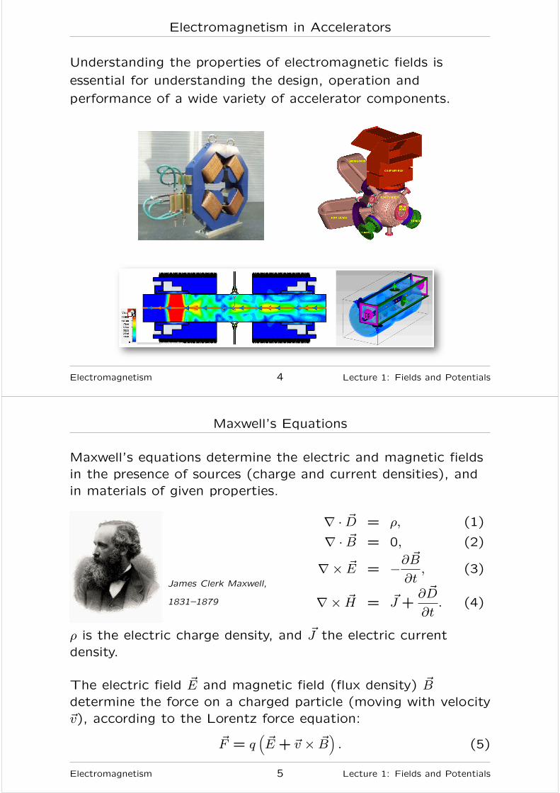
Understanding the properties of electromagnetic fields is
essential for understanding the design, operation and
performance of a wide variety of accelerator components.
Electromagnetism 4 Lecture 1: Fields and Potentials
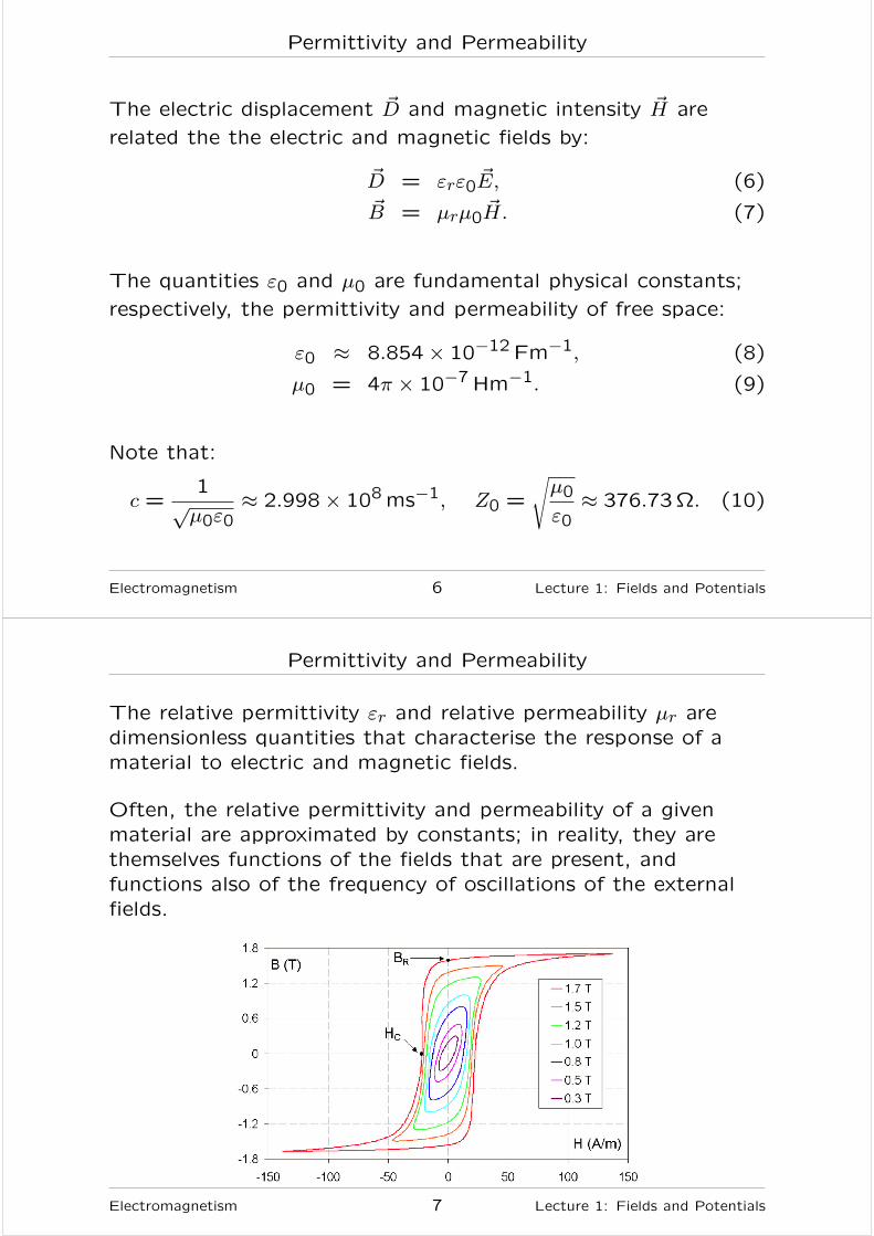
Maxwell’s Equations
Maxwell’s equations determine the electric and magnetic fields
in the presence of sources (charge and current densities), and
in materials of given properties.
James Clerk Maxwell,
1831–1879
∇ · ~D = ρ, (1)
∇ · ~B = 0, (2)
∇× ~E = −∂~B
∂t, (3)
∇× ~H = ~J +∂ ~D
∂t. (4)
ρ is the electric charge density, and ~J the electric current
density.
The electric field ~E and magnetic field (flux density) ~B
determine the force on a charged particle (moving with velocity
~v), according to the Lorentz force equation:
~F = q(
~E + ~v × ~B)
. (5)
Electromagnetism 5 Lecture 1: Fields and Potentials
Permittivity and Permeability
The electric displacement ~D and magnetic intensity ~H are
related the the electric and magnetic fields by:
~D = εrε0 ~E, (6)
~B = µrµ0~H. (7)
The quantities ε0 and µ0 are fundamental physical constants;
respectively, the permittivity and permeability of free space:
ε0 ≈ 8.854× 10⁻¹² Fm−1, (8)
µ0 = 4π × 10−7 Hm−1. (9)
Note that:
c =1
√µ0ε0
≈ 2.998× 10⁸ ms−1, Z0 =
√
µ0
ε0≈ 376.73Ω. (10)
Electromagnetism 6 Lecture 1: Fields and Potentials
Permittivity and Permeability
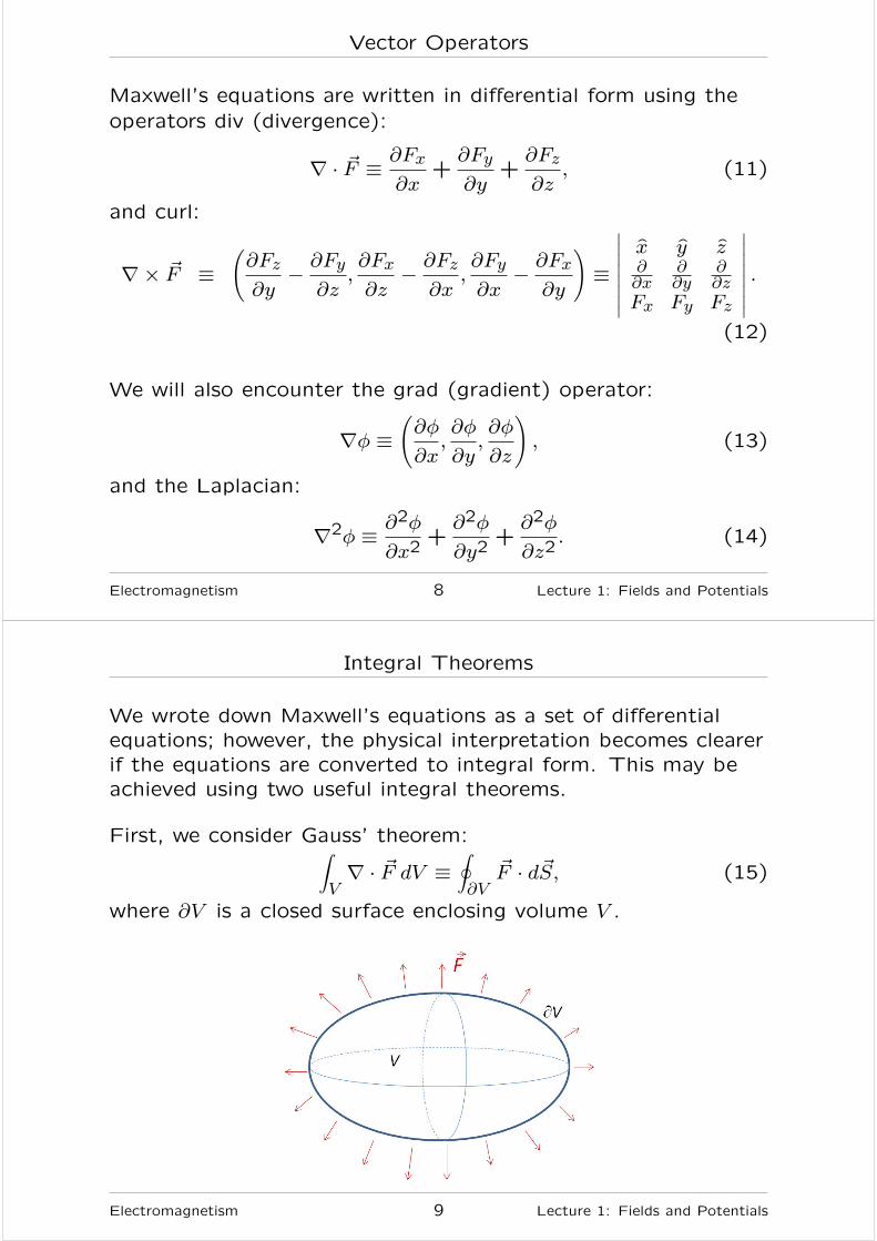
The relative permittivity εr and relative permeability µr are
dimensionless quantities that characterise the response of a
material to electric and magnetic fields.
Often, the relative permittivity and permeability of a given
material are approximated by constants; in reality, they are
themselves functions of the fields that are present, and
functions also of the frequency of oscillations of the external
fields.
Electromagnetism 7 Lecture 1: Fields and Potentials
Vector Operators
Maxwell’s equations are written in differential form using the
operators div (divergence):
∇ · ~F ≡ ∂Fx
∂x+∂Fy
∂y+∂Fz
∂z, (11)
and curl:
∇× ~F ≡(
∂Fz
∂y− ∂Fy
∂z,∂Fx
∂z− ∂Fz
∂x,∂Fy
∂x− ∂Fx
∂y
)
≡
∣
∣
∣
∣
∣
∣
∣
∣
x y z∂∂x
∂∂y
∂∂z
Fx Fy Fz
∣
∣
∣
∣
∣
∣
∣
∣
.
(12)
We will also encounter the grad (gradient) operator:
∇φ ≡(
∂φ
∂x,∂φ
∂y,∂φ
∂z
)
, (13)
and the Laplacian:
∇2φ ≡ ∂2φ
∂x2+∂2φ
∂y2+∂2φ
∂z2. (14)
Electromagnetism 8 Lecture 1: Fields and Potentials
Integral Theorems
We wrote down Maxwell’s equations as a set of differentialequations; however, the physical interpretation becomes clearerif the equations are converted to integral form. This may beachieved using two useful integral theorems.
First, we consider Gauss’ theorem:∫
V∇ · ~F dV ≡
∮
∂V~F · d~S, (15)
where ∂V is a closed surface enclosing volume V .
Electromagnetism 9 Lecture 1: Fields and Potentials
Gauss’ Theorem
Let us apply Gauss’ theorem to Maxwell’s equation:
∇ · ~D = ρ, (16)
to give:∮
∂V~D · d~S =
∫
Vρ dV. (17)
This is the integral form of Maxwell’s equation (1). From this
form, we can find a physical interpretation of Maxwell’s
equation (1). The integral form of the equation tells us that
the electric displacement integrated over any closed surface
equals the electric charge contained within that surface.
Electromagnetism 10 Lecture 1: Fields and Potentials
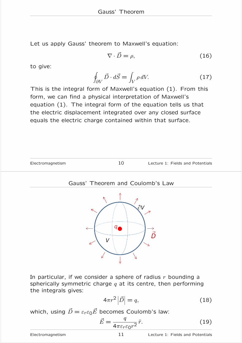
Gauss’ Theorem and Coulomb’s Law
In particular, if we consider a sphere of radius r bounding aspherically symmetric charge q at its centre, then performingthe integrals gives:
4πr2∣
∣
∣
~D∣
∣
∣ = q, (18)
which, using ~D = εrε0 ~E becomes Coulomb’s law:
~E =q
4πεrε0r2r. (19)
Electromagnetism 11 Lecture 1: Fields and Potentials
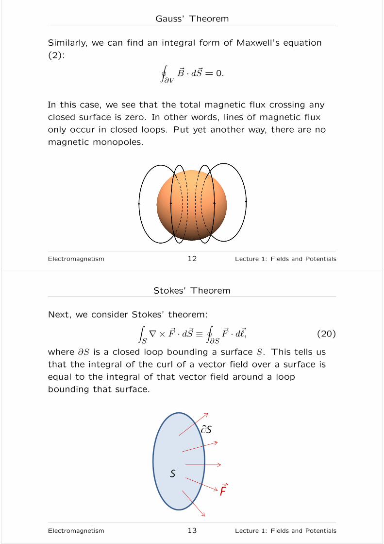
Gauss’ Theorem
Similarly, we can find an integral form of Maxwell’s equation
(2):∮
∂V~B · d~S = 0.
In this case, we see that the total magnetic flux crossing any
closed surface is zero. In other words, lines of magnetic flux
only occur in closed loops. Put yet another way, there are no
magnetic monopoles.
Electromagnetism 12 Lecture 1: Fields and Potentials
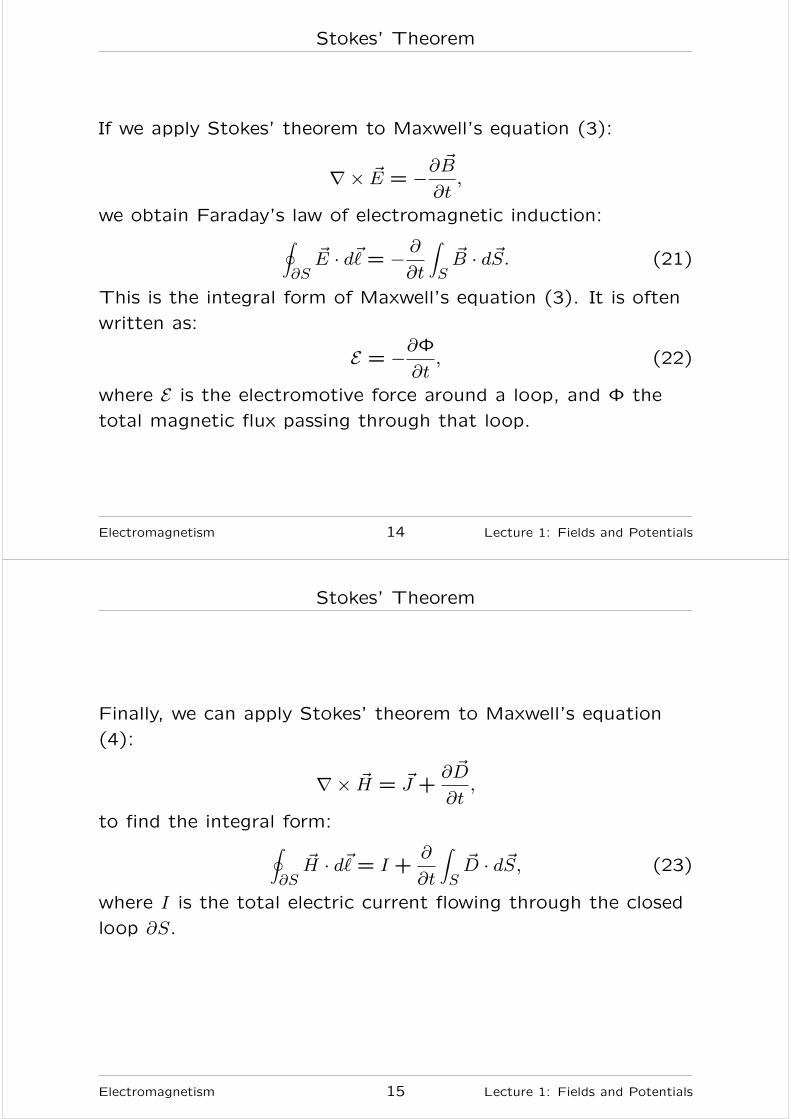
Stokes’ Theorem
Next, we consider Stokes’ theorem:∫
S∇× ~F · d~S ≡
∮
∂S~F · d~, (20)
where ∂S is a closed loop bounding a surface S. This tells us
that the integral of the curl of a vector field over a surface is
equal to the integral of that vector field around a loop
bounding that surface.
Electromagnetism 13 Lecture 1: Fields and Potentials
Stokes’ Theorem
If we apply Stokes’ theorem to Maxwell’s equation (3):
∇× ~E = −∂~B
∂t,
we obtain Faraday’s law of electromagnetic induction:∮
∂S~E · d~= − ∂
∂t
∫
S~B · d~S. (21)
This is the integral form of Maxwell’s equation (3). It is often
written as:
E = −∂Φ∂t, (22)
where E is the electromotive force around a loop, and Φ the
total magnetic flux passing through that loop.
Electromagnetism 14 Lecture 1: Fields and Potentials
Stokes’ Theorem
Finally, we can apply Stokes’ theorem to Maxwell’s equation
(4):
∇× ~H = ~J +∂ ~D
∂t,
to find the integral form:∮
∂S~H · d~= I +
∂
∂t
∫
S~D · d~S, (23)
where I is the total electric current flowing through the closed
loop ∂S.
Electromagnetism 15 Lecture 1: Fields and Potentials
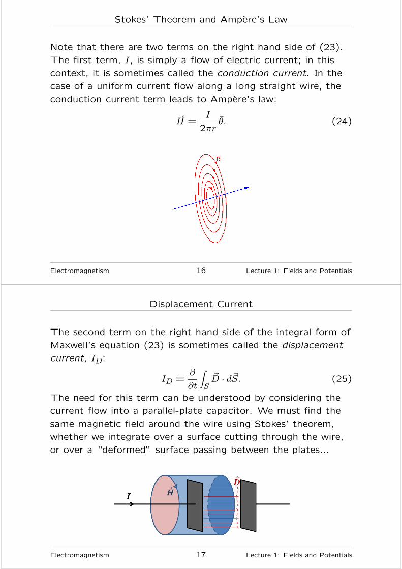
Stokes’ Theorem and Ampere’s Law
Note that there are two terms on the right hand side of (23).
The first term, I, is simply a flow of electric current; in this
context, it is sometimes called the conduction current. In the
case of a uniform current flow along a long straight wire, the
conduction current term leads to Ampere’s law:
~H =I
2πrθ. (24)
Electromagnetism 16 Lecture 1: Fields and Potentials
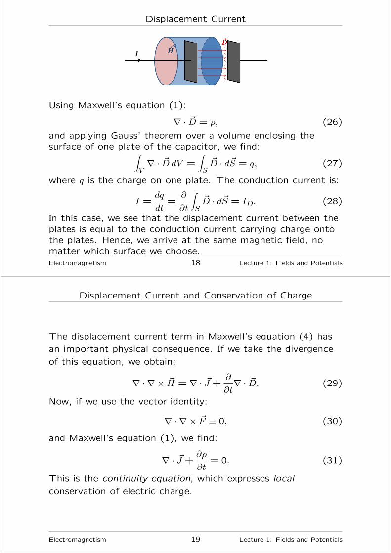
Displacement Current
The second term on the right hand side of the integral form of
Maxwell’s equation (23) is sometimes called the displacement
current, ID:
ID =∂
∂t
∫
S~D · d~S. (25)
The need for this term can be understood by considering the
current flow into a parallel-plate capacitor. We must find the
same magnetic field around the wire using Stokes’ theorem,
whether we integrate over a surface cutting through the wire,
or over a “deformed” surface passing between the plates...
Electromagnetism 17 Lecture 1: Fields and Potentials
Displacement Current
Using Maxwell’s equation (1):
∇ · ~D = ρ, (26)
and applying Gauss’ theorem over a volume enclosing thesurface of one plate of the capacitor, we find:
∫
V∇ · ~D dV =
∫
S~D · d~S = q, (27)
where q is the charge on one plate. The conduction current is:
I =dq
dt=
∂
∂t
∫
S~D · d~S = ID. (28)
In this case, we see that the displacement current between theplates is equal to the conduction current carrying charge ontothe plates. Hence, we arrive at the same magnetic field, nomatter which surface we choose.
Electromagnetism 18 Lecture 1: Fields and Potentials
Displacement Current and Conservation of Charge
The displacement current term in Maxwell’s equation (4) has
an important physical consequence. If we take the divergence
of this equation, we obtain:
∇ · ∇ × ~H = ∇ · ~J +∂
∂t∇ · ~D. (29)
Now, if we use the vector identity:
∇ · ∇ × ~F ≡ 0, (30)
and Maxwell’s equation (1), we find:
∇ · ~J +∂ρ
∂t= 0. (31)
This is the continuity equation, which expresses local
conservation of electric charge.
Electromagnetism 19 Lecture 1: Fields and Potentials
Displacement Current and Conservation of Charge
The physical interpretation of the continuity equation becomes
clearer if we use Gauss’ theorem, to put it into integral form:∫
∂V~J · d~S = − ∂
∂t
∫
Vρ dV. (32)
We see that the rate of decrease of electric charge in a region
V is equal to the total current flowing out of the region
through its boundary, ∂V . Since current is the rate of flow of
electric charge, the continuity equation expresses the local
conservation of electric charge.
Electromagnetism 20 Lecture 1: Fields and Potentials
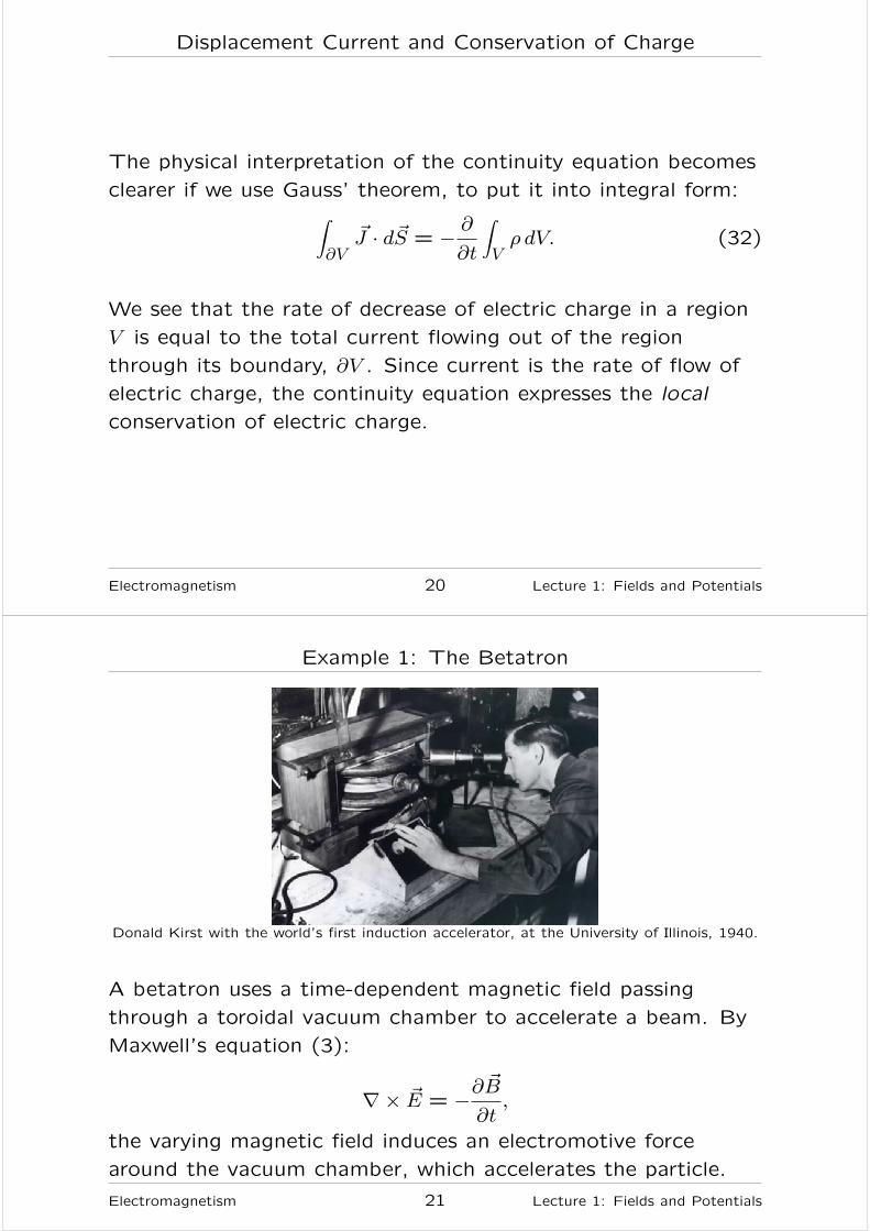
Example 1: The Betatron
Donald Kirst with the world’s first induction accelerator, at the University of Illinois, 1940.
A betatron uses a time-dependent magnetic field passing
through a toroidal vacuum chamber to accelerate a beam. By
Maxwell’s equation (3):
∇× ~E = −∂~B
∂t,
the varying magnetic field induces an electromotive force
around the vacuum chamber, which accelerates the particle.
Electromagnetism 21 Lecture 1: Fields and Potentials
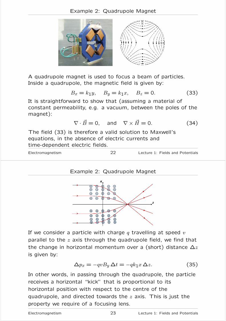
Example 2: Quadrupole Magnet
A quadrupole magnet is used to focus a beam of particles.
Inside a quadrupole, the magnetic field is given by:
Bx = k1y, By = k1x, Bz = 0. (33)
It is straightforward to show that (assuming a material of
constant permeability, e.g. a vacuum, between the poles of the
magnet):
∇ · ~B = 0, and ∇× ~H = 0. (34)
The field (33) is therefore a valid solution to Maxwell’s
equations, in the absence of electric currents and
time-dependent electric fields.
Electromagnetism 22 Lecture 1: Fields and Potentials
Example 2: Quadrupole Magnet
If we consider a particle with charge q travelling at speed v
parallel to the z axis through the quadrupole field, we find that
the change in horizontal momentum over a (short) distance ∆z
is given by:
∆px = −qvBy∆t = −qk1x∆z. (35)
In other words, in passing through the quadrupole, the particle
receives a horizontal “kick” that is proportional to its
horizontal position with respect to the centre of the
quadrupole, and directed towards the z axis. This is just the
property we require of a focusing lens.
Electromagnetism 23 Lecture 1: Fields and Potentials
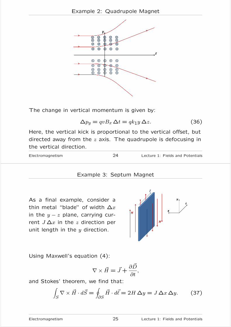
Example 2: Quadrupole Magnet
The change in vertical momentum is given by:
∆py = qvBx∆t = qk1y∆z. (36)
Here, the vertical kick is proportional to the vertical offset, but
directed away from the z axis. The quadrupole is defocusing in
the vertical direction.
Electromagnetism 24 Lecture 1: Fields and Potentials
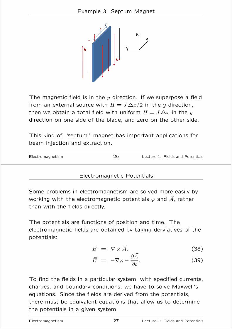
Example 3: Septum Magnet
As a final example, consider a
thin metal “blade” of width ∆x
in the y − z plane, carrying cur-
rent J∆x in the z direction per
unit length in the y direction.
.
Using Maxwell’s equation (4):
∇× ~H = ~J +∂ ~D
∂t,
and Stokes’ theorem, we find that:∫
S∇× ~H · d~S =
∮
∂S~H · d~= 2H∆y = J∆x∆y. (37)
Electromagnetism 25 Lecture 1: Fields and Potentials
Example 3: Septum Magnet
The magnetic field is in the y direction. If we superpose a field
from an external source with H = J∆x/2 in the y direction,
then we obtain a total field with uniform H = J∆x in the y
direction on one side of the blade, and zero on the other side.
This kind of “septum” magnet has important applications for
beam injection and extraction.
Electromagnetism 26 Lecture 1: Fields and Potentials
Electromagnetic Potentials
Some problems in electromagnetism are solved more easily by
working with the electromagnetic potentials ϕ and ~A, rather
than with the fields directly.
The potentials are functions of position and time. The
electromagnetic fields are obtained by taking derviatives of the
potentials:
~B = ∇× ~A, (38)
~E = −∇ϕ− ∂ ~A
∂t. (39)
To find the fields in a particular system, with specified currents,
charges, and boundary conditions, we have to solve Maxwell’s
equations. Since the fields are derived from the potentials,
there must be equivalent equations that allow us to determine
the potentials in a given system.
Electromagnetism 27 Lecture 1: Fields and Potentials
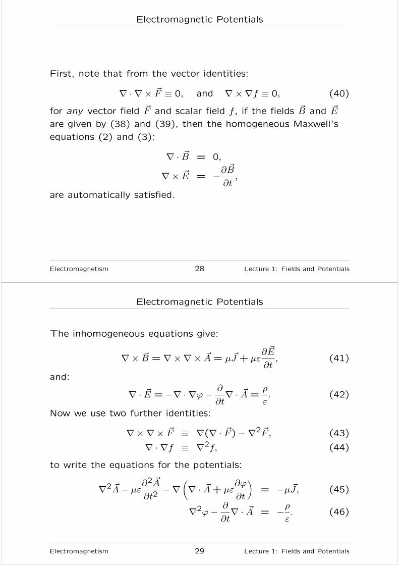
Electromagnetic Potentials
First, note that from the vector identities:
∇ · ∇ × ~F ≡ 0, and ∇×∇f ≡ 0, (40)
for any vector field ~F and scalar field f , if the fields ~B and ~E
are given by (38) and (39), then the homogeneous Maxwell’s
equations (2) and (3):
∇ · ~B = 0,
∇× ~E = −∂~B
∂t,
are automatically satisfied.
Electromagnetism 28 Lecture 1: Fields and Potentials
Electromagnetic Potentials
The inhomogeneous equations give:
∇× ~B = ∇×∇× ~A = µ~J + µε∂ ~E
∂t, (41)
and:
∇ · ~E = −∇ · ∇ϕ− ∂
∂t∇ · ~A =
ρ
ε. (42)
Now we use two further identities:
∇×∇× ~F ≡ ∇(∇ · ~F )−∇2 ~F , (43)
∇ · ∇f ≡ ∇2f, (44)
to write the equations for the potentials:
∇2 ~A− µε∂2 ~A
∂t2−∇
(
∇ · ~A+ µε∂ϕ
∂t
)
= −µ~J, (45)
∇2ϕ− ∂
∂t∇ · ~A = −ρ
ε. (46)
Electromagnetism 29 Lecture 1: Fields and Potentials
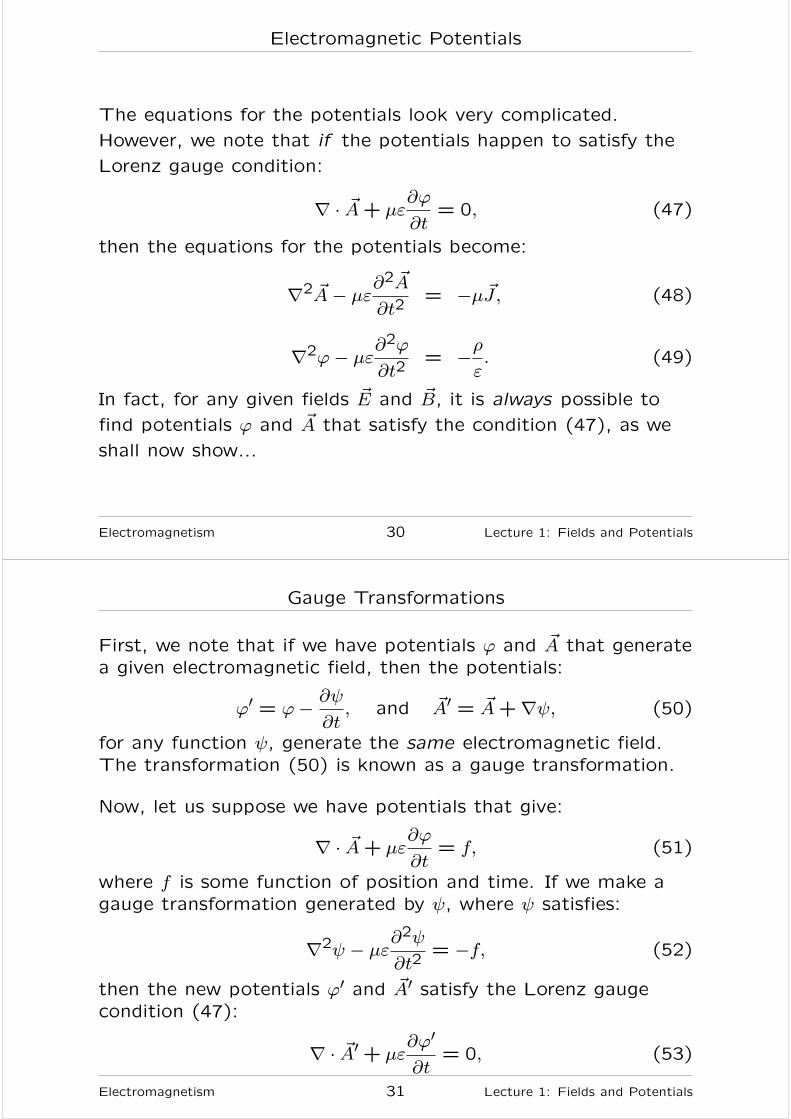
Electromagnetic Potentials
The equations for the potentials look very complicated.
However, we note that if the potentials happen to satisfy the
Lorenz gauge condition:
∇ · ~A+ µε∂ϕ
∂t= 0, (47)
then the equations for the potentials become:
∇2 ~A− µε∂2 ~A
∂t2= −µ~J, (48)
∇2ϕ− µε∂2ϕ
∂t2= −ρ
ε. (49)
In fact, for any given fields ~E and ~B, it is always possible to
find potentials ϕ and ~A that satisfy the condition (47), as we
shall now show...
Electromagnetism 30 Lecture 1: Fields and Potentials
Gauge Transformations
First, we note that if we have potentials ϕ and ~A that generatea given electromagnetic field, then the potentials:
ϕ′ = ϕ− ∂ψ
∂t, and ~A′ = ~A+∇ψ, (50)
for any function ψ, generate the same electromagnetic field.The transformation (50) is known as a gauge transformation.
Now, let us suppose we have potentials that give:
∇ · ~A+ µε∂ϕ
∂t= f, (51)
where f is some function of position and time. If we make agauge transformation generated by ψ, where ψ satisfies:
∇2ψ − µε∂2ψ
∂t2= −f, (52)
then the new potentials ϕ′ and ~A′ satisfy the Lorenz gaugecondition (47):
∇ · ~A′+ µε∂ϕ′
∂t= 0, (53)
Electromagnetism 31 Lecture 1: Fields and Potentials
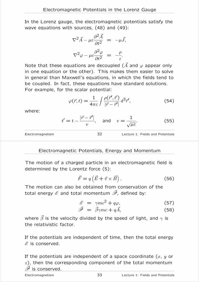
Electromagnetic Potentials in the Lorenz Gauge
In the Lorenz gauge, the electromagnetic potentials satisfy the
wave equations with sources, (48) and (49):
∇2 ~A− µε∂2 ~A
∂t2= −µ~J,
∇2ϕ− µε∂2ϕ
∂t2= −ρ
ε.
Note that these equations are decoupled ( ~A and ϕ appear only
in one equation or the other). This makes them easier to solve
in general than Maxwell’s equations, in which the fields tend to
be coupled. In fact, these equations have standard solutions.
For example, for the scalar potential:
ϕ(~r, t) =1
4πε
∫
ρ(~r′, t′)|~r − ~r′| d
3~r′, (54)
where:
t′ = t−∣
∣~r − ~r′∣
∣
v, and v =
1√µε. (55)
Electromagnetism 32 Lecture 1: Fields and Potentials
Electromagnetic Potentials, Energy and Momentum
The motion of a charged particle in an electromagnetic field is
determined by the Lorentz force (5):
~F = q(
~E + ~v × ~B)
. (56)
The motion can also be obtained from conservation of the
total energy E and total momentum ~P, defined by:
E = γmc2 + qϕ, (57)
~P = ~βγmc+ q ~A, (58)
where ~β is the velocity divided by the speed of light, and γ is
the relativistic factor.
If the potentials are independent of time, then the total energy
E is conserved.
If the potentials are independent of a space coordinate (x, y or
z), then the corresponding component of the total momentum~P is conserved.
Electromagnetism 33 Lecture 1: Fields and Potentials
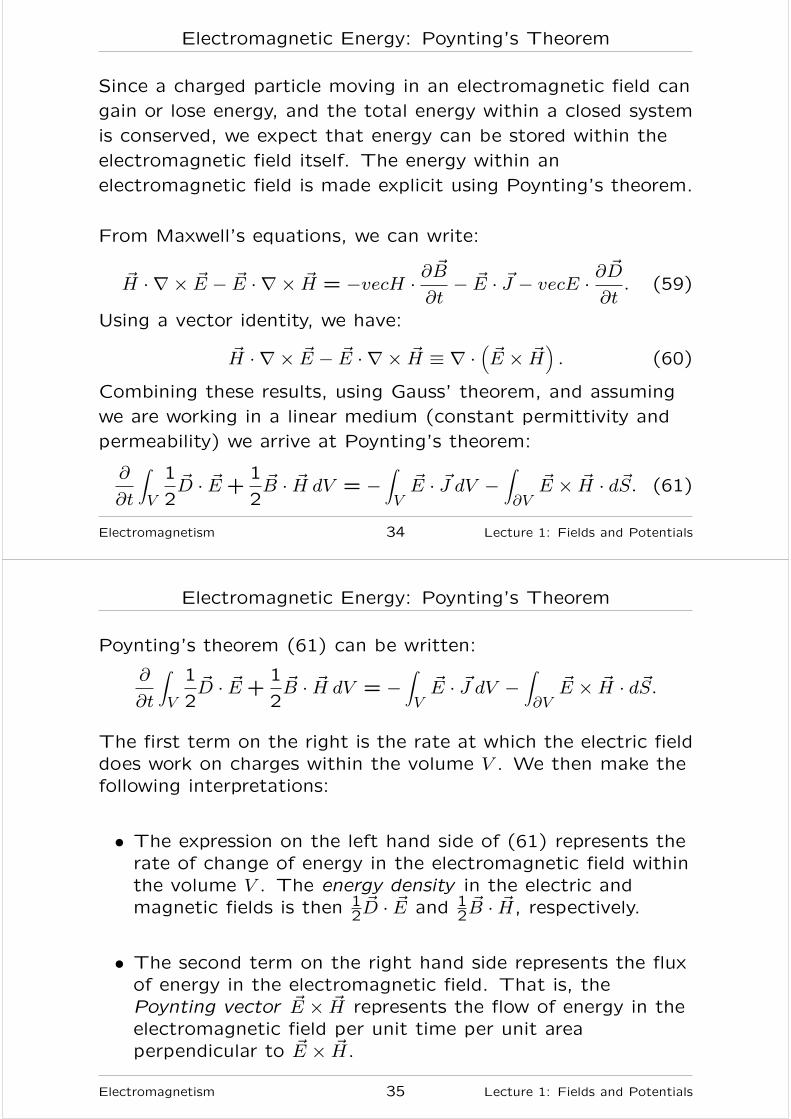
Electromagnetic Energy: Poynting’s Theorem
Since a charged particle moving in an electromagnetic field can
gain or lose energy, and the total energy within a closed system
is conserved, we expect that energy can be stored within the
electromagnetic field itself. The energy within an
electromagnetic field is made explicit using Poynting’s theorem.
From Maxwell’s equations, we can write:
~H · ∇ × ~E − ~E · ∇ × ~H = −vecH · ∂~B
∂t− ~E · ~J − vecE · ∂
~D
∂t. (59)
Using a vector identity, we have:
~H · ∇ × ~E − ~E · ∇ × ~H ≡ ∇ ·(
~E × ~H)
. (60)
Combining these results, using Gauss’ theorem, and assuming
we are working in a linear medium (constant permittivity and
permeability) we arrive at Poynting’s theorem:
∂
∂t
∫
V
1
2~D · ~E +
1
2~B · ~H dV = −
∫
V~E · ~J dV −
∫
∂V~E × ~H · d~S. (61)
Electromagnetism 34 Lecture 1: Fields and Potentials
Electromagnetic Energy: Poynting’s Theorem
Poynting’s theorem (61) can be written:
∂
∂t
∫
V
1
2~D · ~E +
1
2~B · ~H dV = −
∫
V~E · ~J dV −
∫
∂V~E × ~H · d~S.
The first term on the right is the rate at which the electric fielddoes work on charges within the volume V . We then make thefollowing interpretations:
• The expression on the left hand side of (61) represents therate of change of energy in the electromagnetic field withinthe volume V . The energy density in the electric andmagnetic fields is then 1
2~D · ~E and 1
2~B · ~H, respectively.
• The second term on the right hand side represents the fluxof energy in the electromagnetic field. That is, thePoynting vector ~E × ~H represents the flow of energy in theelectromagnetic field per unit time per unit areaperpendicular to ~E × ~H.
Electromagnetism 35 Lecture 1: Fields and Potentials
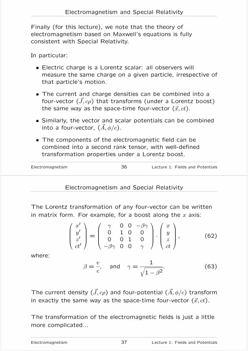
Electromagnetism and Special Relativity
Finally (for this lecture), we note that the theory of
electromagnetism based on Maxwell’s equations is fully
consistent with Special Relativity.
In particular:
• Electric charge is a Lorentz scalar: all observers will
measure the same charge on a given particle, irrespective of
that particle’s motion.
• The current and charge densities can be combined into a
four-vector ( ~J, cρ) that transforms (under a Lorentz boost)
the same way as the space-time four-vector (~x, ct).
• Similarly, the vector and scalar potentials can be combined
into a four-vector, ( ~A, φ/c).
• The components of the electromagnetic field can be
combined into a second rank tensor, with well-defined
transformation properties under a Lorentz boost.
Electromagnetism 36 Lecture 1: Fields and Potentials
Electromagnetism and Special Relativity
The Lorentz transformation of any four-vector can be written
in matrix form. For example, for a boost along the x axis:
x′y′z′ct′
=
γ 0 0 −βγ0 1 0 00 0 1 0−βγ 0 0 γ
·
xyzct
, (62)
where:
β =v
c, and γ =
1√
1− β2. (63)
The current density ( ~J, cρ) and four-potential ( ~A, φ/c) transform
in exactly the same way as the space-time four-vector (~x, ct).
The transformation of the electromagnetic fields is just a little
more complicated...
Electromagnetism 37 Lecture 1: Fields and Potentials
Electromagnetism and Special Relativity
Using index notation, we can write the transformation of a
four-vector as:
x′µ = Λµνxν. (64)
where the indices µ and ν range from 1 to 4.
Note that we use the summation convention, so that a
summation (from 1 to 4) is implied whenever an index appears
twice in any term.
The transformation of the electromagnetic fields can be
deduced from the transformations of the potentials, and the
space-time coordinates. The result is:
F ′µν = ΛµαΛνβF
αβ, (65)
where Fαβ is the matrix:
F =
0 Bz −By −Ex/c−Bz 0 Bx −Ey/cBy −Bx 0 −Ez/cEx/c Ey/c Ez/c 0
. (66)
Electromagnetism 38 Lecture 1: Fields and Potentials
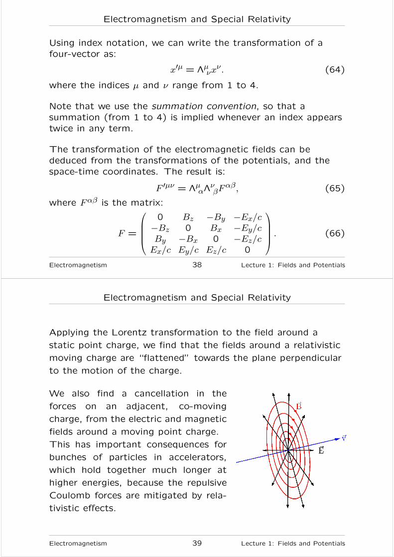
Electromagnetism and Special Relativity
Applying the Lorentz transformation to the field around a
static point charge, we find that the fields around a relativistic
moving charge are “flattened” towards the plane perpendicular
to the motion of the charge.
We also find a cancellation in the
forces on an adjacent, co-moving
charge, from the electric and magnetic
fields around a moving point charge.
This has important consequences for
bunches of particles in accelerators,
which hold together much longer at
higher energies, because the repulsive
Coulomb forces are mitigated by rela-
tivistic effects.
Electromagnetism 39 Lecture 1: Fields and Potentials
Electromagnetism and Special Relativity
Note that any two four-vectors may be combined to form a
Lorentz scalar, using the metric tensor g. For example:
xµxµ ≡ gµνx
νxµ (67)
where:
g =
1 0 0 00 1 0 00 0 1 00 0 0 −1
(68)
is a Lorentz scalar (invariant under a boost).
Note that the metric tensor is used to change an “up” index to
a “down” index (a covariant vector to a contravariant vector).
In any summation over an index, the index should appear once
in the “up” position, and once in the “down” position.
Electromagnetism 40 Lecture 1: Fields and Potentials
Electromagnetism and Special Relativity
To write the equations of electromagnetism in explicitly
covariant form (i.e. in a form where the transformations under
a boost are obvious), we need the four-vector differential
operator:
∂µ =
(
∂
∂x,∂
∂y,∂
∂z,−1
c
∂
∂t
)
. (69)
The second-order differential operator, , is called the
d’Alembertian, and is defined by:
≡ ∂µ∂µ =
∂2
∂x2+
∂2
∂y2+
∂2
∂z2− 1
c2∂2
∂t2. (70)
Electromagnetism 41 Lecture 1: Fields and Potentials
Electromagnetism and Special Relativity
With the covariant quantities we have defined, Maxwell’s
equations may be written:
∂µFµν = −µ0J
ν, (71)
∂λFµν + ∂µF νλ + ∂νFλµ = 0. (72)
The continuity equation may be written as:
∂µJµ = 0. (73)
The fields may be derived from the potentials using:
Fµν = ∂µAν − ∂νAµ. (74)
The Lorenz gauge condition is:
∂µAµ = 0. (75)
In the Lorenz gauge, the potentials satisfy the inhomogeneous
wave equation:
Aµ = −µ0Jµ. (76)
Electromagnetism 42 Lecture 1: Fields and Potentials
Summary
You should be able to:
• write down Maxwell’s equations in differential form, and use
Gauss’ and Stokes’ theorems to change them to integral
form;
• discuss the physical interpretation of Maxwell’s equations,
with some examples relevant to accelerators;
• explain how the dynamics of particles in an accelerator are
governed by the Lorentz force;
• state the relationship between the electromagnetic
potentials and the electromagnetic field, and explain how
the potentials can be used in solving electrodynamical
problems;
• derive Poynting’s theorem, and explain the physical
significance of the different terms;
• write down the equations of electromagnetism in explicitly
covariant form.
Electromagnetism 43 Lecture 1: Fields and Potentials