Revisiting reservoir storage–yield relationships …engineering.tufts.edu/cee/people/vogel/documents/revisiting...Revisiting reservoir storage–yield relationships using a global

www.elsevier.com/locate/advwatres

Advances in Water Resources 30 (2007) 1858–1872

Revisiting reservoir storage–yield relationships using a globalstreamflow database

Thomas A. McMahon a,*, Geoffrey G.S. Pegram b, Richard M. Vogel c, Murray C. Peel a

a Department of Civil and Environmental Engineering, The University of Melbourne, Vic. 3010, Australiab Civil Engineering Programme, University of KwaZulu-Natal, Durban, South Africa

c Department of Civil and Environmental Engineering, Tufts University, MA, USA

Received 9 November 2006; received in revised form 9 February 2007; accepted 9 February 2007Available online 21 February 2007

Abstract

Annual and monthly streamflows for 729 rivers from a global data set are used to assess the adequacy of five techniques to estimatethe relationship between reservoir capacity, target draft (or yield) and reliability of supply. The techniques examined are extended deficitanalysis (EDA), behaviour analysis, sequent peak algorithm (SPA), Vogel and Stedinger empirical (lognormal) method and Phien empir-ical (Gamma) method. In addition, a technique to adjust SPA using annual flows to account for within-year variations is assessed. Of ournine conclusions the key ones are, firstly, EDA is a useful procedure to estimate streamflow deficits and, hence, reservoir capacity for agiven reliability of supply. Secondly, the behaviour method is suitable to estimate storage but has limitations if an annual time step isadopted. Thirdly, in contrast to EDA and behaviour which are based on time series of flows, if only annual statistics are available,the Vogel and Stedinger empirical method compares favorably with more detailed simulation approaches.� 2007 Elsevier Ltd. All rights reserved.

Keywords: Reservoir theory; Storage–yield; Sequent peak; Behaviour analysis; Extended deficit analysis; Water supply

1. Introduction

This paper explores the relationship between reservoirstorage and yield using monthly and annual streamflowdata that cover most regions of the globe. We examine res-ervoir capacity as the dependent variable rather than draft(yield) because most of the procedures are formulated inthis way. However, as the relationship between storage sizeand reservoir yield needs to be specified in a reservoir stor-age–yield analysis it is a straightforward exercise to inter-change these two variables.

The history of reservoir storage–yield analysis is a richone with the first important method by Rippl [36] proposednearly 125 years ago, followed by the works of Hazen [15]

0309-1708/$ - see front matter � 2007 Elsevier Ltd. All rights reserved.

doi:10.1016/j.advwatres.2007.02.003

* Corresponding author. Tel.: +61 3 8344 7731; fax: +61 3 8344 6215.E-mail addresses: [email protected] (T.A. McMa-

hon), [email protected] (G.G.S. Pegram), [email protected](R.M. Vogel), [email protected] (M.C. Peel).

and Sudler [38]. However, it was not until the 1950s that aserious effort was made to bring some mathematical rigourinto the process with the activities of Hurst [16], Moran [27]and his colleagues Gani [7], Prabhu [34], Ghosal [8], Lang-bein [19] and Lloyd [21]. With the introduction of stochas-tic data generation in the early sixties, emphasis movedback to Rippl type techniques focusing on the sequent peakalgorithm [39]. During the sixties, seventies and eightiesseveral useful critical period techniques by Alexander [5],Gould [10], and Hardison [13] were proposed as well asmany empirical generalizations based on stochastic dataand simulation including Gould [9], Vogel and Stedinger[44] and Phien [33]. The contributions of Pegram [30] andBuchberger and Maidment [6] are important as they pro-vide exact solutions for specific storage–yield conditions.Considerations of reservoir performance and sustainabilitywere also a feature of the eighties and nineties especiallyin the works of Hashimoto et al. [14], Loucks [22] andSimonovic [37]. Throughout this latter period Klemes’s

mailto:[email protected]




T.A. McMahon et al. / Advances in Water Resources 30 (2007) 1858–1872 1859

publications [18] provided a theoretical setting for theapproaches discussed in this paper.

One impetus for this paper was the availability of a glo-bal data set of monthly and annual streamflow that hadbeen subjected to a rigorous quality assessment and cov-ered most regions of the world. This allowed the authorsto explore how well five very different storage–yield tech-niques (Extended Deficit Analysis, behaviour analysis,sequent peak analysis, Vogel and Stedinger procedureand Phien’s empirical method) handled the wide range ofstreamflow characteristics that were found in the globaldata set, which would provide a practical setting for thetesting of the procedures.

The analysis focuses on hypothetical storages at thestream gauging station for each river and was restrictedto estimating a constant annual yield (75% draft) and reli-ability characteristics using the Standard Operating Policyin which demand is satisfied if there is sufficient water in thereservoir, otherwise the reservoir empties. Including draftratios other than 75% and seasonal drafts in the analysiswould have extended the exercise beyond the availableresources.

Following this introduction, Section 2 describes thecharacteristics of large reservoirs located in Australia,South Africa and the United States. Next, we outline thebackground theory and application for five reservoir stor-age–yield (S–Y) techniques that are currently used in prac-tice. The global annual and monthly streamflow data setsused to compare and contrast the S–Y methods aredescribed in Section 4. In Sections 5 and 6, we apply thetechniques to the global data set and explore the differencesamong the procedures to identify their attributes and inad-equacies. Summary comments are made in Section 7 andrelevant conclusions are drawn in Section 8.

2. Some reservoir characteristics

The three key variables in S–Y analysis are active reser-voir capacity S, draft or yield D, and reliability of draft,often expressed in terms of T, the average return period(in years) of at least one failure to supply the demand inan interval (month or year). Several measures of reservoirperformance other than reliability are also used, namelyvulnerability and resilience, but these tend to be of second-ary importance and will not be addressed in this paper. Tosimplify theoretical analysis active reservoir or storagecapacity, which is defined as the difference between totalstorage capacity at full supply level and dead storage (thevolume of water held below the lowest off-take) is used.The capacity is expressed either as a ratio of mean annualinflow S/l, or as a ratio of the standard deviation of annualinflows S/r, the latter ratio is known as the standardizedcapacity C. S/l is a useful measure for practitionersbecause it represents the maximum number of years ofwater held in storage, while, for many theoretical studies,it is useful to standardize the capacity with respect to r.Draft is also expressed as the ratio of mean annual inflow,

a = D/l, often as a percentage. Another parameter (m) thatincludes draft is known as the standardized net inflow [16]or drift [30,40] and is defined as follows:

m ¼ 1� aCv

; ð1Þ

where Cv = r/l is the coefficient of variation of annual in-flows. Hazen [15] was the first to adopt this parameter in hisanalysis of reservoir capacities for municipal water supplies.He denoted the parameter by the symbol ‘k’ but did not coina term to describe it. This is a useful parameter which en-ables one to capture the impact of both streamflow variabil-ity, Cv, and reservoir yield (a) on reservoir storage.

The total capacities of individual reservoirs world-wideare listed in publications like ICOLD World Register ofDams [17]. However, typical values of capacity, expressedas S/l or S/r, and draft are not readily available. Never-theless, there are several sources of data which haveallowed us to build a picture of the variation of these res-ervoir parameters across three countries – Australia, SouthAfrica and the United States. For example, the statisticsbased on 48 Australian reservoirs are as follows [23]:

• Of the 48 large reservoirs, the median value of drift is0.66. Thirty-six reservoirs (75%) have a value of drift(m) < 1.0.

• Draft ratios vary between �90% to less than 10% of themean annual streamflow (MAF) into the reservoirs. Themedian value is 47%.

• For the same 48 reservoirs, reservoir capacities vary frommore than 6 · MAF to some being <0.25 · MAF or interms of annual standard deviation from >10 · annualstandard deviation (annual r) to <0.25 · annual r. Themedian size of the reservoirs is 1.28 · MAF or in termsof standardized capacity 1.71 · annual r.

In South Africa, withdrawal rules are typically opti-mized in systems of interconnected reservoirs, so there isonly a small subset of those with their own complete (notincremental) catchments:

• For 12 of the larger stand-alone reservoirs, the mediandrift is 0.63, of which one has a drift of 1.01, the remain-der have drifts between 0.25 and 0.91.

• For these 12 reservoirs, draft ratios vary between 14%and 90% of MAF: the median value is 29%.

• For the same 12 South African reservoirs, capacitiesvary from more than 3.3 · MAF to some being<0.7 · MAF or in terms of annual standard deviationfrom >6.8 · annual r to <0.63 · annual r. The mediansize of the reservoirs is 1.22 · MAF or in terms of stan-dardized capacity 1.20 · annual r.

Graf [11] reviews the general characteristics of over75000 dams in the United States and Vogel et al. [46] eval-uate the hydrologic characteristics of a smaller subset ofjust over 5000 of those dams. Dam behaviour differs quite

Table 1Values of drift or standardized inflow, m, as a function of draft ratio a andannual Cv

Annual Cv a (%)

25 50 75 90 100

0.1 7.5 5.0 2.5 1.0 0

0.5 1.5 1 0.5 0.2 0

1.0 0.75 0.5 0.25 0.1 0

2.0 0.375 0.25 0.125 0.05 0

Drift (m) = (1 � a)/Cv.Values indicated in italics denotes carry-over storage (0 6 m 6 Cv) [42].

1860 T.A. McMahon et al. / Advances in Water Resources 30 (2007) 1858–1872

dramatically in eastern and western regions of the US dueto differences in hydrologic variability

• Boxplots of drift for thousands of reservoirs are pre-sented in [46] illustrating that east of the Mississippiriver drift is generally greater than 1 whereas it is gener-ally less than 1 in western regions.

• Drafts range from around 40% to 95% of MAF in someeastern regions and are nearly uniformly distributed insome western regions.

• Storage capacities are generally less than the MAF inthe eastern regions, but range from nearly zero to nearly5xMAF in some western regions.

In summary, the large reservoirs in Australia and SouthAfrica exhibit similar characteristics – typically, reservoircapacities are about 11/4 times mean annual flow, draftratios vary from about 10% to 90%, and the median mag-nitude of drift is about 2/3. In US, large regional differ-ences are observed with the eastern regions beingcharacterized by higher drafts and smaller reservoir capac-ities than in the western regions.

Values of drift as a function of a and Cv are shown inTable 1 and, for all practical purposes, cover the range ofvalues found globally. As a rough guide, reservoirs withm < Cv are considered to operate usually as over-year orcarry-over storage reservoirs (these are reservoirs in whichpart of the stored water is carried over from one year andused in subsequent years), whereas those where m P Cvare classified as within-year systems and would be usuallyexpected to spill annually [46]. Vogel and Bolognese [41]had suggested m P 1 as the guide for within-year storage.As noted by the shading in Table 1 the two guidelines,m P 1 and m P Cv, are consistent. Montaseri and Adeloye[26] argue that other variables in addition to m and Cv,such as reliability, may be needed to classify reservoirs ascarry-over or within-year storages. We emphasize thatthe classification between systems dominated by within-year or over-year behaviour is more of a continuum, thana sharp distinction, given by any set of rules.

3. Reviewing some key approaches

This section compares five approaches (other than sto-chastic simulation) – Extended deficit analysis, behaviour

analysis, sequent peak algorithm, Vogel and Stedingerempirical (lognormal) method and Phien empirical(Gamma) method – that are currently available for reser-voir storage–yield analysis. We begin by describing eachmethod along with its attributes and limitations.

3.1. Extended deficit analysis

The Extended Deficit Analysis (EDA) was proposed byPegram [32] as a simple technique to compute the averagerecurrence interval of reservoir deficits (in other words, themean recurrence interval between emptiness) directly fromthe historical inflows, excluding net evaporation and otherlosses. (Evaporation can be handled externally [23]).

The method is based on the storage equation applied toa semi-infinite reservoir (one that can spill but never empty)to determine the capacity S required to provide a chosendraft of given reliability:

Zt ¼ min½0; Zt�1 þ Qt � Dt�ðfor simultaneous inflows and draftsÞ; ð2Þ

Zt ¼ min½0; Zt�1 þ Qt� � Dt

ðfor inflows and drafts out of phaseÞ; ð3Þ

where Zt and Zt� 1 are storage values (60) at times t andt � 1, (initial storage is assumed full: Z0 = 0), Qt is the in-flow and Dt is the draft during the interval (t � 1, t). Theanalysis computes the minimum storage between spills(i.e., when Z = 0) as positive deficits:

Def j ¼ �min½St between spills j� 1 and j�; j ¼ 1; 2; . . . ; r;

ð4Þ

noting that the spill j = 0 occurs at t = 0 because Z0 = 0, bydefinition. In applying the method here, the Pegram proce-dure was slightly modified by incorporating the lowest stor-age experienced between the last spill and the end of therecord, although it is not technically a deficit by the defini-tion of Eq. (4).

Because the deficits Defj, j = 1,2, . . ., r + 1 are separatedby spills (except the r + 1th deficit), they form a renewalprocess and are therefore mutually independent. FollowingTroutman [40], who showed that for a semi-infinite storagefed by inflows with a < 1 (or m > 0) the maximum deficitasymptotically has an Extreme Value Type 1 (EV1) orGumbel distribution, the ‘‘larger’’ deficits can thereforebe considered to be EV1 distributed.

Once the series of r + 1 deficits is obtained, they areranked from largest (i = 1) to smallest (i = r + 1) and foreach deficit a sample average recurrence interval is calcu-lated using Gringorten’s plotting position [12]:

T ¼ N þ 0:12

i� 0:44; ð5Þ

where N is the number of years in the historical record andi is the rank of the deficit. For each value of T, the EV1 re-duced variate, y, is calculated from


y ¼ � ln � ln 1� 1

T

� �� : ð6Þ

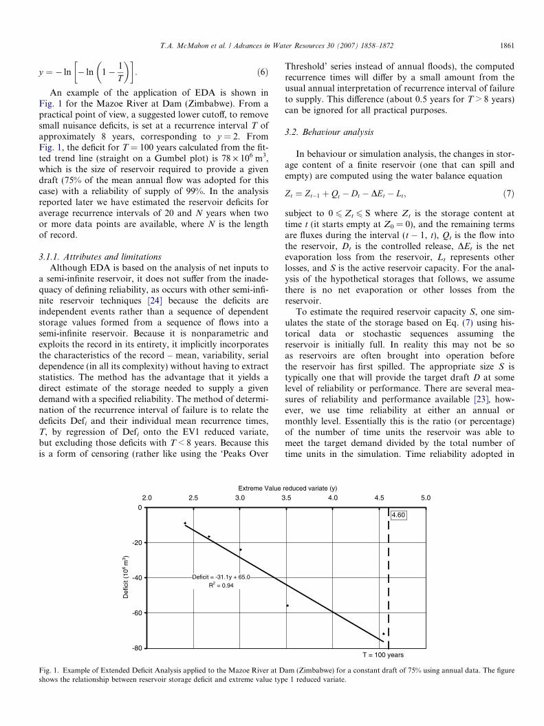
An example of the application of EDA is shown inFig. 1 for the Mazoe River at Dam (Zimbabwe). From apractical point of view, a suggested lower cutoff, to removesmall nuisance deficits, is set at a recurrence interval T ofapproximately 8 years, corresponding to y = 2. FromFig. 1, the deficit for T = 100 years calculated from the fit-ted trend line (straight on a Gumbel plot) is 78 · 106 m3,which is the size of reservoir required to provide a givendraft (75% of the mean annual flow was adopted for thiscase) with a reliability of supply of 99%. In the analysisreported later we have estimated the reservoir deficits foraverage recurrence intervals of 20 and N years when twoor more data points are available, where N is the lengthof record.

3.1.1. Attributes and limitations

Although EDA is based on the analysis of net inputs toa semi-infinite reservoir, it does not suffer from the inade-quacy of defining reliability, as occurs with other semi-infi-nite reservoir techniques [24] because the deficits areindependent events rather than a sequence of dependentstorage values formed from a sequence of flows into asemi-infinite reservoir. Because it is nonparametric andexploits the record in its entirety, it implicitly incorporatesthe characteristics of the record – mean, variability, serialdependence (in all its complexity) without having to extractstatistics. The method has the advantage that it yields adirect estimate of the storage needed to supply a givendemand with a specified reliability. The method of determi-nation of the recurrence interval of failure is to relate thedeficits Defi and their individual mean recurrence times,T, by regression of Defi onto the EV1 reduced variate,but excluding those deficits with T < 8 years. Because thisis a form of censoring (rather like using the ‘Peaks Over

Deficit = -31.1y + 65.0R2 = 0.94

-80

-60

-40

-20

02.0 2.5 3.0 3

Extreme Value

Def

icit

(106

m3 )

Fig. 1. Example of Extended Deficit Analysis applied to the Mazoe River at Dshows the relationship between reservoir storage deficit and extreme value typ

Threshold’ series instead of annual floods), the computedrecurrence times will differ by a small amount from theusual annual interpretation of recurrence interval of failureto supply. This difference (about 0.5 years for T > 8 years)can be ignored for all practical purposes.

3.2. Behaviour analysis

In behaviour or simulation analysis, the changes in stor-age content of a finite reservoir (one that can spill andempty) are computed using the water balance equation

Zt ¼ Zt�1 þ Qt � Dt � DEt � Lt; ð7Þ

subject to 0 6 Zt 6 S where Zt is the storage content attime t (it starts empty at Z0 = 0), and the remaining termsare fluxes during the interval (t � 1, t), Qt is the flow intothe reservoir, Dt is the controlled release, DEt is the netevaporation loss from the reservoir, Lt represents otherlosses, and S is the active reservoir capacity. For the anal-ysis of the hypothetical storages that follows, we assumethere is no net evaporation or other losses from thereservoir.

To estimate the required reservoir capacity S, one sim-ulates the state of the storage based on Eq. (7) using his-torical data or stochastic sequences assuming thereservoir is initially full. In reality this may not be soas reservoirs are often brought into operation beforethe reservoir has first spilled. The appropriate size S istypically one that will provide the target draft D at somelevel of reliability or performance. There are several mea-sures of reliability and performance available [23], how-ever, we use time reliability at either an annual ormonthly level. Essentially this is the ratio (or percentage)of the number of time units the reservoir was able tomeet the target demand divided by the total number oftime units in the simulation. Time reliability adopted in

.5 4.0 4.5 5.0reduced variate (y)

4.60

T = 100 years

am (Zimbabwe) for a constant draft of 75% using annual data. The figuree 1 reduced variate.


behaviour analysis and most often in practice is differentfrom the reliability statements adopted by the other meth-ods considered in this study.

The yield estimate from this calculation is known assteady state yield in contrast to the firm yield estimatedby the sequent peak algorithm which is discussed next.Because the historical record length is usually too shortto estimate steady state conditions (see the discussion thatfollows), McMahon and Adeloye [23] have introduced theterm pseudo-steady state to describe behaviour analysisyield estimates based on historical data lengths.


A behaviour (or simulation) analysis is a simple andvisual procedure to estimate storage capacity and is notrestricted by the characteristics of the inflows. Unlike someof the analytical approaches, evaporation and operatingrules that are a function of reservoir storage levels can beeasily taken into account [23].

Depending on the length of the annual inflow data, stor-age size for high reliabilities cannot be estimated. Forexample, with 50 years of data, the required storage sizefor 99% annual time reliability (1/100 years probability offailure) cannot be estimated.

Based on stochastically generated annual streamflows,Pretto et al. [35] found that biases occur in the mean andhigher order quantiles of storage estimates before the esti-mated storage size converges to a stationary value after along sequence (typically 1000 years or more). Adeloyeet al. [2] noted that by restricting the shortfall during fail-ures the biases largely disappear.

3.3. Sequent peak algorithm

A number of variants of the sequent peak algorithm(SPA) are available that accommodate storage dependentlosses. In this paper, we restrict our analysis to the applica-tion of the basic SPA to a single reservoir. Assuming theinitial storage in a semi-infinite reservoir is zero (in otherwords, the reservoir starts full as in EDA), we apply thewater balance Eq. (2) for all years or months in the stream-flow record of length N:

Zt ¼ min½0; Zt�1 þ Qt � Dt�; ð8Þwhere Zt is the storage (60) at time t (again Z0 = 0), and Dt

and Qt are the draft and the inflow during the interval(t � 1, t). If ZN 5 Z0 we continue with Eq. (8) for the con-catenated inflow sequence. The required active reservoircapacity is given by:

S ¼ �minðZtÞ over all t ¼ 1; 2; . . . ;Nðor 2N if ZN 6¼ Z0Þ:ð9Þ


Using the historical inflow data, SPA computes the stor-age required to provide the firm yield, which is the yieldthat can be met over a particular planning period with

no failure. This approach has been widely used in the Uni-ted States and elsewhere. Furthermore, the design capacityof many reservoirs world-wide has been determined usingeither the Rippl [36] graphical method or the SPA whichis a numerical version of that technique. Borrowing fromEDA, the steady-state reliability associated with S isroughly 1 � 1/N, though since only one failure is allowedover the N-year period, this is a very poor estimate ofsteady-state reliability.

As SPA is equivalent to the Rippl graphical masscurve procedure [36], it suffers from the same limitations.First, the estimated storage is based on the critical his-toric low flow sequence and says little about the reliabil-ity (expressed as a probability) of meeting the targetdraft. Second, fluxes (including evaporation) dependenton storage content cannot be taken into account in thesimple SPA procedure. However, Lele [20] and Adeloyeand Montaseri [1] offer more complex algorithms to over-come this inadequacy.

3.4. Vogel and Stedinger empirical procedure

Vogel and Stedinger (V–S) [44] showed that for a reser-voir system fed by AR(1) lognormal streamflows, the stan-dardized storage C (capacity divided by the standarddeviation) for a failure-free operation (SPA approach) isa random variable described by a three-parameter Lognor-mal distribution. The form of the V–S relationship is:

Sp ¼ r½#s þ expðl‘ þ zpr‘Þ�; ð10Þ

where Sp is the pth quantile of the distribution of requiredreservoir capacity for 100% failure-free operation over aspecified planning period N, zp is the standardized Normalvariate at p%, r is the standard deviation of annual stream-flows, l‘ and r‘ are mean and standard deviation of thelogarithms of the storages defined in Eqs. (11) and (12),and #s is the lower-bound of the storage. The momentsl‘ and r‘ are computed as follows:

l‘ ¼ ln ðls � #sÞ 1þ r2s

ðls � #sÞ2

!�0:524

35; ð11Þ

r2‘ ¼ ln 1þ r2

s

ðls � #sÞ2

" #; ð12Þ

where ls and rs are the mean (expected value) and standarddeviation of the untransformed (real space) storage capac-ity S.

Vogel and Stedinger [44] carried out extensive MonteCarlo simulations (streamflows were based on an AR(1)log-normal model) within the ranges 0.2 6 Cv 6 0.5,0.1 6 m 6 1, 0 6 q 6 0.5 and 20 6 N years 6100, resultingin the following equations to compute the parameters inEqs. (10)–(12).

l0s ¼ expðaþ bmÞacmmðdqþeNÞN ðfþg lnðmÞÞ 1þ q1� q

� �h ln½N �

; ð13Þ


r02s ¼ exp aþ baþ cNmþ d

Nþ e

m

� �1þ q1� q

� �� N f ln½m� 1þ q

1� q

� �g ln½N �

;

ð14Þ

#0s ¼ aqþ bN þ cð1þ qÞð1� qÞ

� �ln½m�

þ N d þ emþ fm ln½N � þ g ln

1þ q1� q

� �� ; ð15Þ

where a through h are the empirical parameters based onsimulation, a is the target draft ratio D/l, and q is thelag-one serial correlation of annual streamflows. For eachequation a separate set of parameters is required, giving atotal of 22; they are listed in [23,44]. Analogous regres-sions are given for the case of AR(1) normal inflows in[41].


The Vogel and Stedinger empirical procedure estimatesthe expected value and variance of SPA reservoir storagecapacity assuming both the inflows to the reservoir andthe standardized storages are lognormally distributed.Although the method is based on six equations and 22parameters, its application is straightforward.

Being an empirical procedure, it should really only beapplied within the range of values of m, Cv, N and q thatwere used to define the 22 parameters. However, as notedin Section 5.4.2, the results of applying the technique tothe set of global rivers suggests it can be used across the fullrange of rivers with caution.

Evaporation is not explicitly taken into account but canbe handled externally (see for example McMahon and Ade-loye [23]).

3.5. Phien empirical procedure

Phien [33] also used the SPA procedure to explore thedistribution of the required reservoir capacities butadopted the Gamma rather than lognormal distributionto define stochastically generated reservoir inflows. Phien’scriteria were based on drift, lag-one serial correlation andrecord-length as follows: 0 6 m 6 0.50, 0 6 q 6 0.5 and20 6 N years 650. This is a more limited data set thanadopted by Vogel and Stedinger [44]. Based on the simu-lated results, Phien developed several empirical relation-ships, far simpler in form than the empirical models in[41,44]; his equations for the expected value and the stan-dard deviation of standardized storages are:

lS ¼ 1:467N 0:466 1þ q1� q

� �0:5311� m1þ m

� �2:047

; ð16Þ

rS ¼ 1:787N 0:243 1þ q1� q

� �0:8551� m1þ m

� �2:198

; ð17Þ

where lS and rS are the mean (expected value) and stan-dard deviation of the storage values.


In contrast to the V–S procedure, Phien’s methodassumes the annual streamflows are Gamma distributedand uses only two simple equations to compute theexpected value and the variance of standardized reservoircapacities. However, the range of the characteristics ofstreamflows is more limited than those used in the V–Smethod. Furthermore, as noted in Section 5.4.2, the proce-dure should not be used outside the range specified.

Following Section 4, in which the global set of stream-flow records are described, the above methods for estimat-ing required reservoir capacities are applied to the globaldata.

4. Streamflow data

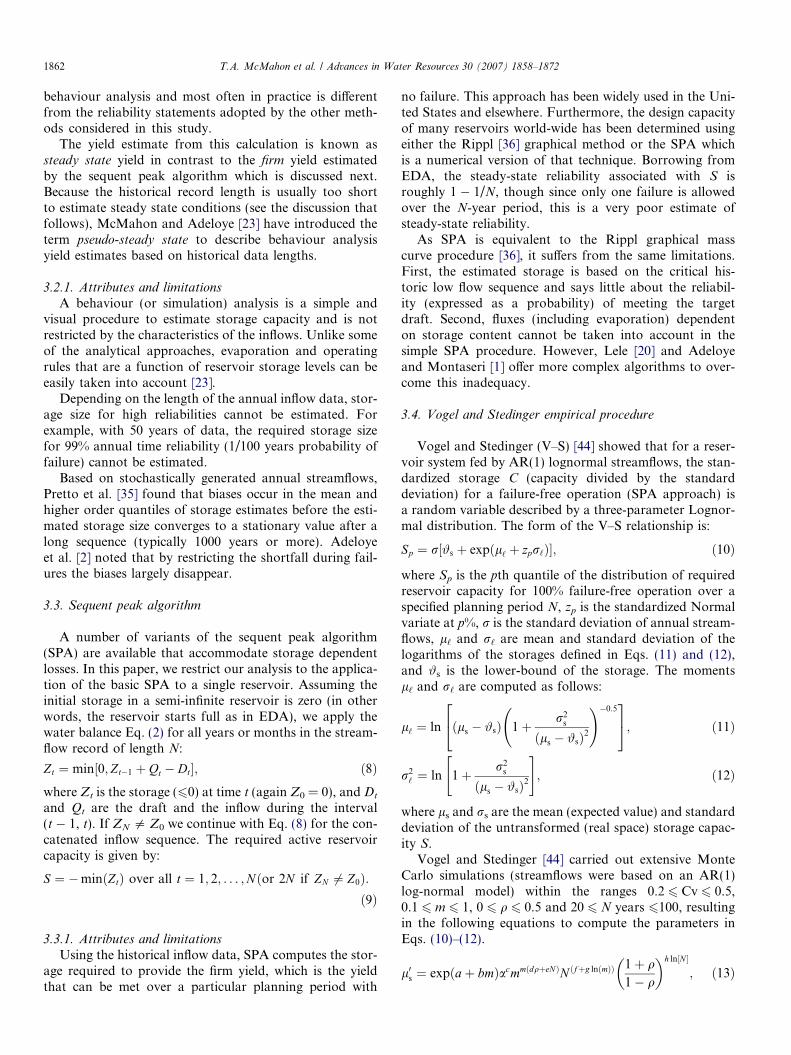
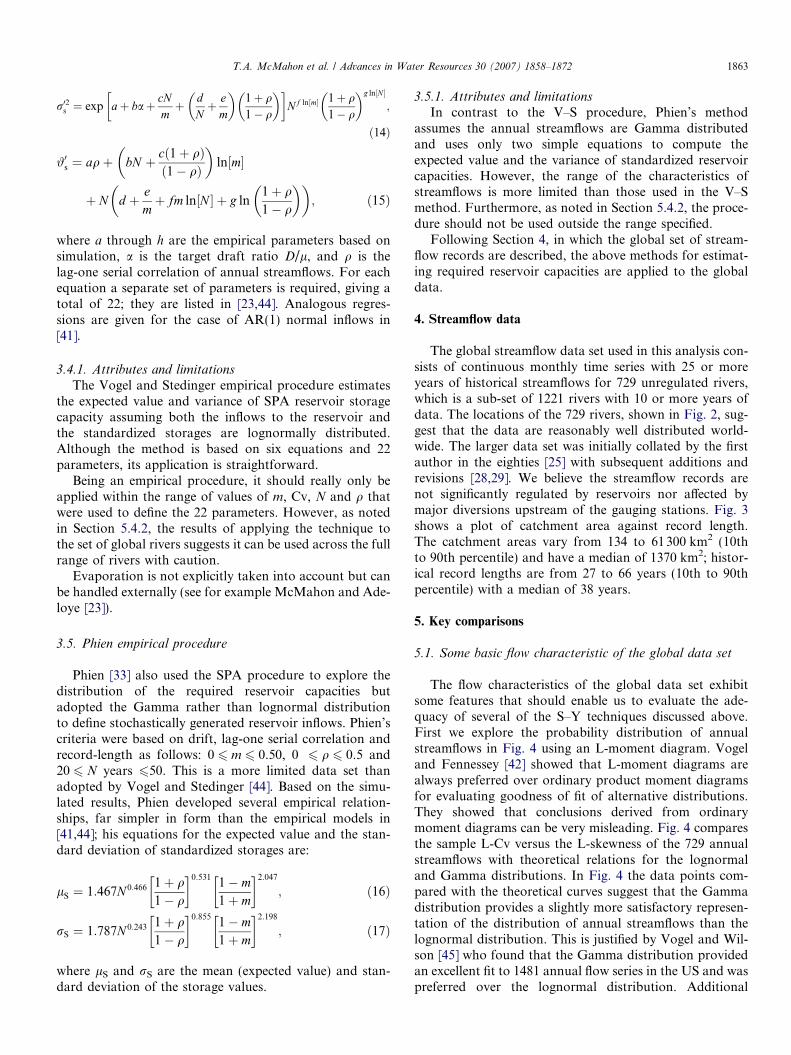
The global streamflow data set used in this analysis con-sists of continuous monthly time series with 25 or moreyears of historical streamflows for 729 unregulated rivers,which is a sub-set of 1221 rivers with 10 or more years ofdata. The locations of the 729 rivers, shown in Fig. 2, sug-gest that the data are reasonably well distributed world-wide. The larger data set was initially collated by the firstauthor in the eighties [25] with subsequent additions andrevisions [28,29]. We believe the streamflow records arenot significantly regulated by reservoirs nor affected bymajor diversions upstream of the gauging stations. Fig. 3shows a plot of catchment area against record length.The catchment areas vary from 134 to 61300 km2 (10thto 90th percentile) and have a median of 1370 km2; histor-ical record lengths are from 27 to 66 years (10th to 90thpercentile) with a median of 38 years.

5. Key comparisons

5.1. Some basic flow characteristic of the global data set

The flow characteristics of the global data set exhibitsome features that should enable us to evaluate the ade-quacy of several of the S–Y techniques discussed above.First we explore the probability distribution of annualstreamflows in Fig. 4 using an L-moment diagram. Vogeland Fennessey [42] showed that L-moment diagrams arealways preferred over ordinary product moment diagramsfor evaluating goodness of fit of alternative distributions.They showed that conclusions derived from ordinarymoment diagrams can be very misleading. Fig. 4 comparesthe sample L-Cv versus the L-skewness of the 729 annualstreamflows with theoretical relations for the lognormaland Gamma distributions. In Fig. 4 the data points com-pared with the theoretical curves suggest that the Gammadistribution provides a slightly more satisfactory represen-tation of the distribution of annual streamflows than thelognormal distribution. This is justified by Vogel and Wil-son [45] who found that the Gamma distribution providedan excellent fit to 1481 annual flow series in the US and waspreferred over the lognormal distribution. Additional

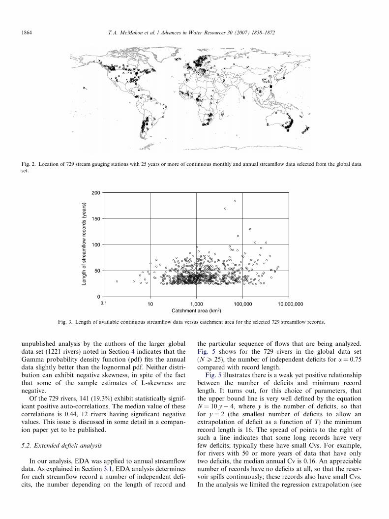
Fig. 2. Location of 729 stream gauging stations with 25 years or more of continuous monthly and annual streamflow data selected from the global dataset.

0

50

100

150

200

10 1,000 100,000 10,000,000Catchment area (km2)

Leng

th o

f str

eam

flow

rec

ords

(ye

ars)

0.1

Fig. 3. Length of available continuous streamflow data versus catchment area for the selected 729 streamflow records.


unpublished analysis by the authors of the larger globaldata set (1221 rivers) noted in Section 4 indicates that theGamma probability density function (pdf) fits the annualdata slightly better than the lognormal pdf. Neither distri-bution can exhibit negative skewness, in spite of the factthat some of the sample estimates of L-skewness arenegative.

Of the 729 rivers, 141 (19.3%) exhibit statistically signif-icant positive auto-correlations. The median value of thesecorrelations is 0.44, 12 rivers having significant negativevalues. This issue is discussed in some detail in a compan-ion paper yet to be published.

5.2. Extended deficit analysis

In our analysis, EDA was applied to annual streamflowdata. As explained in Section 3.1, EDA analysis determinesfor each streamflow record a number of independent defi-cits, the number depending on the length of record and

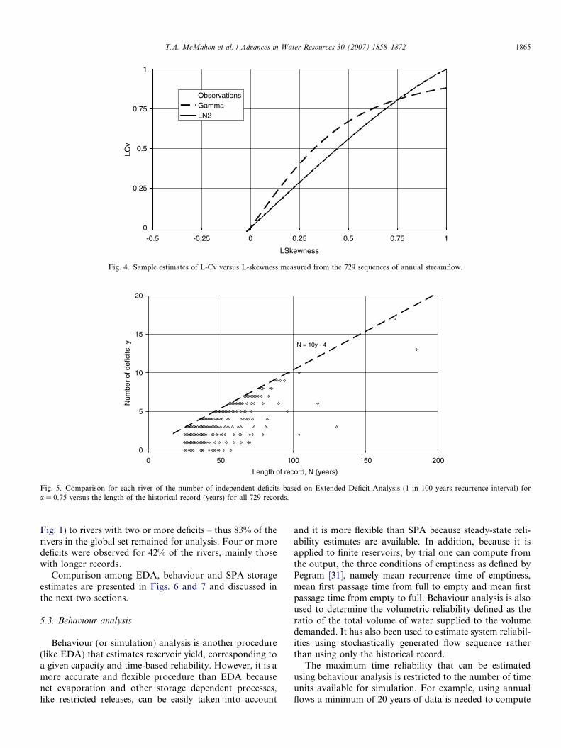
the particular sequence of flows that are being analyzed.Fig. 5 shows for the 729 rivers in the global data set(N P 25), the number of independent deficits for a = 0.75compared with record length.

Fig. 5 illustrates there is a weak yet positive relationshipbetween the number of deficits and minimum recordlength. It turns out, for this choice of parameters, thatthe upper bound line is very well defined by the equationN = 10 y � 4, where y is the number of deficits, so thatfor y = 2 (the smallest number of deficits to allow anextrapolation of deficit as a function of T) the minimumrecord length is 16. The spread of points to the right ofsuch a line indicates that some long records have veryfew deficits; typically these have small Cvs. For example,for rivers with 50 or more years of data that have onlytwo deficits, the median annual Cv is 0.16. An appreciablenumber of records have no deficits at all, so that the reser-voir spills continuously; these records also have small Cvs.In the analysis we limited the regression extrapolation (see

0

0.25

0.5

0.75

1

-0.5 -0.25 0 0.25 0.5 0.75 1

LSkewness

LCv

ObservationsGammaLN2

Fig. 4. Sample estimates of L-Cv versus L-skewness measured from the 729 sequences of annual streamflow.

0

5

10

15

20

0 50 100 150 200

Length of record, N (years)

Num

ber

of d

efic

its, y

N = 10y - 4

Fig. 5. Comparison for each river of the number of independent deficits based on Extended Deficit Analysis (1 in 100 years recurrence interval) fora = 0.75 versus the length of the historical record (years) for all 729 records.


Fig. 1) to rivers with two or more deficits – thus 83% of therivers in the global set remained for analysis. Four or moredeficits were observed for 42% of the rivers, mainly thosewith longer records.

Comparison among EDA, behaviour and SPA storageestimates are presented in Figs. 6 and 7 and discussed inthe next two sections.

5.3. Behaviour analysis

Behaviour (or simulation) analysis is another procedure(like EDA) that estimates reservoir yield, corresponding toa given capacity and time-based reliability. However, it is amore accurate and flexible procedure than EDA becausenet evaporation and other storage dependent processes,like restricted releases, can be easily taken into account

and it is more flexible than SPA because steady-state reli-ability estimates are available. In addition, because it isapplied to finite reservoirs, by trial one can compute fromthe output, the three conditions of emptiness as defined byPegram [31], namely mean recurrence time of emptiness,mean first passage time from full to empty and mean firstpassage time from empty to full. Behaviour analysis is alsoused to determine the volumetric reliability defined as theratio of the total volume of water supplied to the volumedemanded. It has also been used to estimate system reliabil-ities using stochastically generated flow sequence ratherthan using only the historical record.

The maximum time reliability that can be estimatedusing behaviour analysis is restricted to the number of timeunits available for simulation. For example, using annualflows a minimum of 20 years of data is needed to compute

10

1,000

100,000

10 1,000 100,000

Behaviour analysis (106 m3)

Ext

ende

d D

efic

it A

naly

sis

(106

m3 )

0.10.1

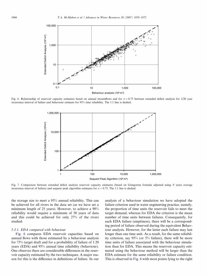
Fig. 6. Relationship of reservoir capacity estimates based on annual streamflows and for a = 0.75 between extended deficit analysis for 1/20 yearrecurrence interval of failure and behaviour estimate for 95% time reliability. The 1:1 line is dashed.

1

100

10,000

1,000,000

1 100 10,000 1,000,000

Sequent Peak Algorithm (106 m3)

Ext

ende

d D

efic

it A

naly

sis

(106

m3 )

Fig. 7. Comparison between extended deficit analysis reservoir capacity estimates (based on Gringorten formula adjusted using N years averagerecurrence interval of failure) and sequent peak algorithm estimates for a = 0.75. The 1:1 line is dashed.


the storage size to meet a 95% annual reliability. This canbe achieved for all rivers in the data set (as we have set aminimum length of 25 years). However, to achieve a 98%reliability would require a minimum of 50 years of dataand this could be achieved for only 27% of the riversstudied.

5.3.1. EDA compared with behaviour

Fig. 6 compares EDA reservoir capacities based onannual flows with those estimated by a behaviour analysisfor 75% target draft and for a probability of failure of 1:20years (EDA) and 95% annual time reliability (behaviour).One observes there are considerable differences in the reser-voir capacity estimated by the two techniques. A major rea-son for this is the difference in definitions of failure. In our

analysis of a behaviour simulation we have adopted thefailure criterion used in water engineering practice, namely,the proportion of time units the reservoir fails to meet thetarget demand, whereas for EDA the criterion is the meannumber of time units between failures. Consequently, foreach EDA failure (emptiness), there will be a correspond-ing period of failure observed during the equivalent Behav-iour analysis. However, for the latter each failure may lastlonger than one time unit. As a result, for the same reliabil-ity criterion, say 95% (or 5% failure), there will be moretime units of failure associated with the behaviour simula-tion than for EDA. This means the reservoir capacity esti-mated using the behaviour method will be larger than theEDA estimate for the same reliability or failure condition.This is observed in Fig. 6 with most points lying to the right


of the 1:1 line. For example, for 75% target draft, therequired reservoir capacity estimated by behaviour com-pared with EDA varies from being 28% larger for a10 · 106 m3 hypothetical reservoir to 86% larger for a10000 · 106 m3 hypothetical reservoir.

5.4. Sequent peak algorithm

The SPA is explored in some depth as it is used widelythroughout the world to estimate S–Y relationships. Inthe SPA analysis that follows, a = 0.75 has been adopted.

5.4.1. SPA compared with EDA

Fig. 7 compares the storage estimates based on an SPAanalysis versus EDA estimates where, for the latter, therecurrence interval to specify the deficit is based on anadjustment of the record length N using the Gringortenformula (Eq. (5)). Despite the fact that the techniques havedifferent theoretical bases, the storage estimates of the twoprocedures for the 599 rivers are virtually identical as con-firmed by the exceptionally high correlation (SpearmanRank Correlation = 0.999).

5.4.2. Empirical and computed estimates of SPA

To provide further insight into the SPA approach, wehave compared the storage estimates by the Vogel and Ste-dinger [44] and the Phien [33] empirical models outlined inSections 3.4 and 3.5 (both of which estimate the SPA-basedstorage for a given firm yield) with the SPA values deter-mined from annual flows in the global data set.

Initially, the Vogel and Stedinger (V–S) estimates werecompared with the SPA estimates for the rivers that fallwithin the limitations: 0.1 6 m 6 1.0, 20 6 N 6 100,0 6 q 6 0.5 and 0.1 6 Cv 6 0.5 [44]. Of the 729 rivers inthe global data set, 221 (30%) fulfilled these conditions.In applying the V–S method we used Eq. (13) which allows

10

1,000

100,000

10

SPA storage based

SP

A s

tora

ge b

ased

on

Vog

el &

Ste

ding

er (

106 m

3 )

0.10.1

Fig. 8. Expectation of reservoir capacity estimates based on empirical Vogelestimates computed from annual data for a = 0.75. (Applicable range 0.1 6dashed.

one to compute the expected value of the standardized stor-age (defined as the estimated mean capacity divided by thestandard deviation of annual inflows).

The results of the comparison are shown in Fig. 8 whichcan be considered as an independent test of the V–S model.Although analysis of the regression equation in log spaceindicates that the slope (0.977) is significantly differentfrom one, the figure does suggest an overall satisfactoryfit. Compared with reservoir capacities estimated usingthe historical data, the V–S model underestimates by about3% and 16% when using volumes of 10 · 106 m3 and1000 · 106 m3, respectively, for comparison. It would bedifficult to confirm whether the minor differences observedin Fig. 8 are due to the fact that we are comparing a singleSPA estimate based on historical flows to an expected valuegiven by Eq. (13) or due to some other cause, for example,the fact that the annual flows may be better described by aGamma distribution than a lognormal distribution which isthe assumption in the V–S model. An analysis to identifythis small bias is outside the scope of this paper.

Given the satisfactory fit of the V–S model in Fig. 8,we have plotted in Fig. 9 the storage estimates basedon the V–S model compared with the SPA estimatesusing the entire global data set. The slope of the regres-sion equation in log space (without intercept) is 0.969compared with 0.977 in Fig. 8. Given that 70% of the riv-ers are outside the parameter ranges used to develop thecoefficients for the model, the figure suggests the modelcan be used with due caution over the full range of flow,data length and drift values. However, it should be notedthat, for large storages, the V–S method underestimatesconsiderably. For example, for an SPA storage of10000 · 106 m3, the trend-line suggests that V–S underes-timates storage by 32%.

In Fig. 10, we compare the Phien model (Eq. (16)) fora = 0.75 with SPA estimates for rivers from the global data

1,000 100,000

on annual flows (106 m3)

and Stedinger Eq. [44] compared with individual sequent peak algorithmm 6 1.0, 0 6 q 6 0.5, 20 6 N 6 100 and 0.1 6 Cv 6 0.5) The 1:1 line is

1

100

10,000

1,000,000

1 100 10,000 1,000,000

SPA estimates based on annual flows (106 m3)

SP

A e

stim

ates

bas

ed o

n V

ogel

& S

tedi

nger

(10

6 m3 )

0.01

0.01

Fig. 9. Comparison between Vogel and Stedinger empirical equation estimates of reservoir capacity compared with sequent peak algorithm estimatescomputed from the global data set of annual flows for a = 0.75. The 1:1 line is dashed.


set that cover the following range of conditions for whichthe Phien empirical equation was developed: 0 6 m 6

0.50, 0 6 q 6 0.5 and 20 6 N years 6 50. Only 19% of the729 global rivers meet these conditions. Overall, the modelunderestimates the storages by about 25%, and the regres-sion slope (0.952) is significantly different from one at the5% level of significance. When applied to all of the globalrivers, the method severely underestimates the reservoircapacities, on average by about 80%, and we therefore rec-ommend it not be applied outside the range of parametersupon which it is based.

6. Storage estimates based on monthly and annual data

The discussion to date has focused on adopting annualstreamflow to estimate reservoir capacities. In the case

1

10

100

1000

10000

100000

1 10 100

SPA storage based

SP

A s

tora

ge b

ased

on

Phi

en (

106 m

3 )

Fig. 10. Reservoir capacity estimates based on empirical Phien equation [33] cofor a = 0.75. (Applicable range 0 6 m 6 0.5, 0 6 q 6 0.5 and 20 6 N 6 50). T

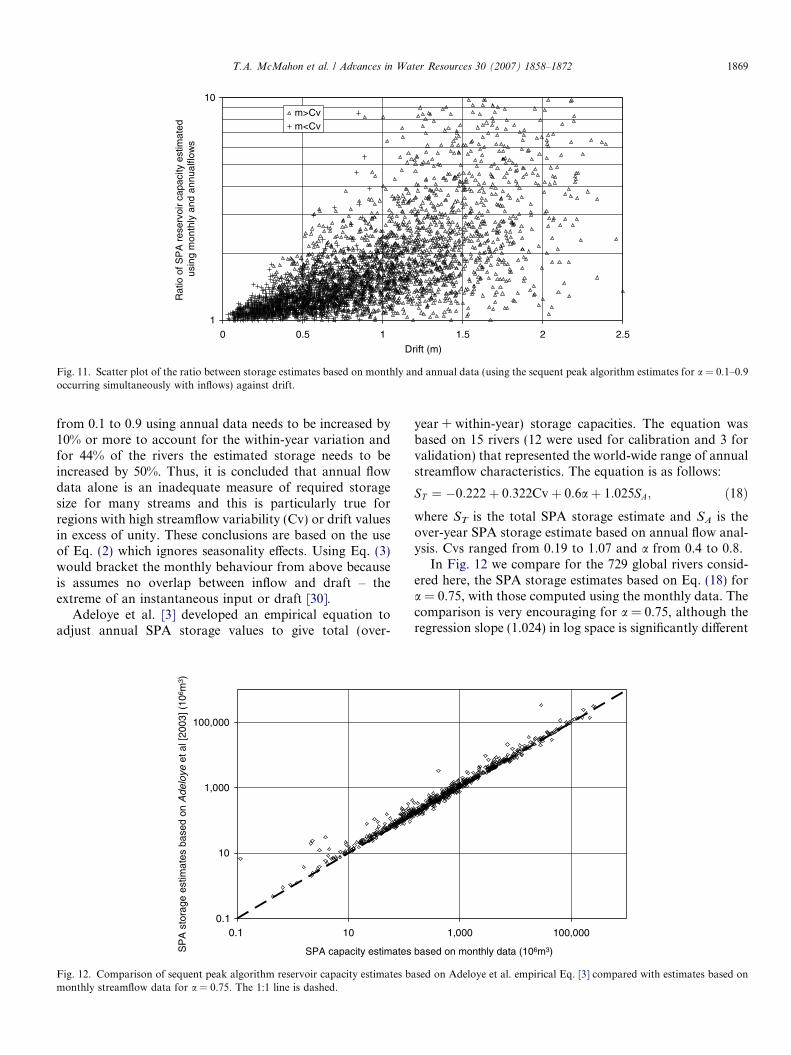
where within-year storage is an important component ofreservoir capacity, monthly data should be used or anappropriate adjustment made to the capacities estimatedusing annual streamflows. To explore how significant thesedifferences might be, we compare for the global data set inFig. 11 the reservoir capacities computed using annual data(Sann) with those estimates from monthly data (Smon) usingSPA analysis. In the figure the ratio of the SPA reservoircapacity computed from monthly flows to that based onannual flows is plotted against drift. The figure also showsseparately Smon/Sann values for m > Cv from m < Cv. Asexpected the majority of values of Smon/Sann for m < Cv fallin the range of the monthly to annual storage ratios of 1–1.5with corresponding drift m values between 0 and 0.75.

The results show that for 87% of the rivers in the globaldata set, the estimated storage requirements for a ranging

1000 10000 100000

on annual flows (106m3)

mpared with sequent peak algorithm estimates computed from annual datahe 1:1 line is dashed.

1

10

0 0.5 1 1.5 2 2.5

Drift (m)

Rat

io o

f SP

A r

eser

voir

capa

city

est

imat

ed

usin

g m

onth

ly a

nd a

nnua

lflow

s

m>Cvm<Cv

Fig. 11. Scatter plot of the ratio between storage estimates based on monthly and annual data (using the sequent peak algorithm estimates for a = 0.1–0.9occurring simultaneously with inflows) against drift.


from 0.1 to 0.9 using annual data needs to be increased by10% or more to account for the within-year variation andfor 44% of the rivers the estimated storage needs to beincreased by 50%. Thus, it is concluded that annual flowdata alone is an inadequate measure of required storagesize for many streams and this is particularly true forregions with high streamflow variability (Cv) or drift valuesin excess of unity. These conclusions are based on the useof Eq. (2) which ignores seasonality effects. Using Eq. (3)would bracket the monthly behaviour from above becauseis assumes no overlap between inflow and draft – theextreme of an instantaneous input or draft [30].

Adeloye et al. [3] developed an empirical equation toadjust annual SPA storage values to give total (over-

10

1,000

100,000

10

SPA capacity estimatesSP

A s

tora

ge e

stim

ates

bas

ed o

n A

delo

ye e

t al [

2003

] (10

6 m3 )

0.10.1

Fig. 12. Comparison of sequent peak algorithm reservoir capacity estimates bmonthly streamflow data for a = 0.75. The 1:1 line is dashed.

year + within-year) storage capacities. The equation wasbased on 15 rivers (12 were used for calibration and 3 forvalidation) that represented the world-wide range of annualstreamflow characteristics. The equation is as follows:

ST ¼ �0:222þ 0:322Cvþ 0:6aþ 1:025SA; ð18Þwhere ST is the total SPA storage estimate and SA is theover-year SPA storage estimate based on annual flow anal-ysis. Cvs ranged from 0.19 to 1.07 and a from 0.4 to 0.8.

In Fig. 12 we compare for the 729 global rivers consid-ered here, the SPA storage estimates based on Eq. (18) fora = 0.75, with those computed using the monthly data. Thecomparison is very encouraging for a = 0.75, although theregression slope (1.024) in log space is significantly different

1,000 100,000

based on monthly data (106m3)

ased on Adeloye et al. empirical Eq. [3] compared with estimates based on


from one. For reservoir capacities of 10 · 106, 1000 · 106

and 100000 · 106 m3, Eq. (18) overestimates the total stor-age using monthly data by 37%, 19% and 4%, respectively.Because of the bias in the equation that is represented bythese results, analysts need to use care in using Eq. (18)to estimate the total capacity of smaller storages.

7. Summary comments

A review of the literature suggests this is the first paperin which several reservoir capacity–yield techniques havebeen compared using a large number of representative riv-ers from a global data set. In the past, comparisons havebeen based on data for only a few rivers or for rivers froma restricted geographical area. The five techniques exam-ined herein represent the two general approaches adoptedfor examining the relationship between reservoir capacityand yield. The two approaches [43] are the no-failure firmyield approach, which is the yield that can be met over aparticular planning period with no failure, represented bythe sequent peak algorithm (and the Vogel and Stedingerand Phien empirical methods) and the steady state yieldapproaches represented by the Extended Deficit Analysisand behaviour analysis.

Before we completed these analyses the authors had lit-tle idea of the level of variation in reservoir capacity esti-mates one could expect between the various techniqueswhen applied to actual river flow data that cover the globalrange of annual streamflow characteristics. To determinestandard errors of estimation in regression analyses likethose in Figs. 7, 8 and 10, a basic assumption is that theregression residuals are normally distributed. Of the threefigures, this assumption is violated only for Fig. 7, but webelieve the degree of non-normality in conjunction withthe large sample size of 599 values in this case provides suf-ficient confidence [4, p. 109] to carryout the following com-parison. Based on the regressions between the two log axesin Figs. 7, 8 and 10 without intercept terms, the followingstandard errors of estimates can be computed in log spaceusing

ffiffiffiffiffiffiffiffiffiffiffiffiffiffiffiffiffiffiffiffiffiffiffiexpðs2Þ � 1

p[13], where s is the standard deviation

of the model residuals when the model is fit in log space,as follows:

Fig. 7 (EDA versus SPA) ±8.7%Fig. 8 (V&S SPA versus SPA from restricted data)±39.4%Fig. 10 (Phien SPA versusu SPA from restricted data)±43.3%

These results suggest that when either of the empiricalmethods V&S or Phien are used, one should be able toachieve standard errors of estimate less than about ±40%.

In water resources system planning, empirical equationslike Eqs. (13) and (16) are often used for initial hydrologicassessment of a range of potential reservoir sites. Althoughthese errors appear large (this is the first time values havebeen computed for a large data set), their magnitudes are

not inconsistent with, for example, errors in mean flow esti-mates for highly variable rivers.

8. Conclusions

A number of conclusions follow from this assessment ofthe application of five reservoir storage–yield techniques –extended deficit analysis, behaviour analysis, sequent peakalgorithm, Vogel and Stedinger empirical method andPhien empirical method – to estimate the capacity of hypo-thetical reservoirs located on 729 rivers distributed globallyand also from previous research results. The rivers with atleast 25 years of continuous monthly streamflow data coverthe range of statistical characteristics observed world-wide.The following conclusions have been reached:

1. Seventy five percent of large Australian reservoirs and91% of large South African reservoirs have values ofdrift m < 1. In the eastern US roughly 50% of the damshave drift <1 whereas in the western US approximately75% of the dams have drift <1.

2. For the same set of Australian and South African reser-voirs, the median value of draft ratio is approximately47% and 29% respectively, and median storage size is1.28 and 1.22 · MAF respectively or, in terms of stan-dardized capacity, 1.71 and 1.20 · annual r, respectively.

3. Unlike other procedures based on semi-infinite reser-voirs fed by historical flows, Extended Deficit Analysis(EDA) provides a simple, but theoretically rigorous,estimate of storage size in terms of recurrence intervalof failure for a specified draft.

4. Ninteen percent of the rivers in the global data set havestatistically significant positive lag-one auto-correlationsfor which the median estimated value is 0.44.

5. We found the Extended Deficit Analysis to be a usefulprocedure to estimate storage for a given draft ratio a.However, because we restricted the analyses to riversyielding at least two deficits, which the method requires,the technique was limited to 83% of the global rivers.

6. Behaviour analysis was found to be a suitable procedureto estimate reservoir capacity. However, at the annualtime step it is restricted by the length of data. For exam-ple, to estimate a capacity for 98% annual time reliabil-ity, at least 50 years of data are required which isavailable for only 27% of the global rivers consideredhere.

7. Overall, the Vogel and Stedinger empirical equations[44] led to a satisfactory agreement when compared toSPA estimates based on historical streamflows. Usingdata within the range for which Vogel and Stedingerempirical equations were developed, the procedureunder-estimates the SPA capacities by between 3% and16% compared with those estimated using the historicalstreamflows. When applied to all the global rivers (manyoutside the range for which the model was developed),the storage estimates were satisfactory, except that largestorages may be underestimated by up to 32%.


8. The Phien model [33] underestimates the storages byabout 25% within its specified range. The model per-formed poorly when applied to the whole data set,underestimating storages by up to 80%.

9. We note that, as a general rule, storages computed usingannual data severely underestimate the storage capacitycomputed when using monthly streamflows whenm > Cv and only moderately when m < Cv. If monthlydata are not available, a total storage capacity can beobtained using the Adeloye et al. [3] empirical equationwhich provides a reasonable correction to obtain com-bined within-year and over-year storage needs.

Acknowledgements

We would like to thank the Department of Civil andEnvironmental Engineering, the University of Melbourneand the Australian Research Council grant DP0449685for financially supporting this research. Our originalstreamflow data set was enhanced by additional datafrom the Global Runoff Data Centre (GRDC) in Kob-lenz, Germany. Streamflow data for Taiwan and NewZealand were also provided by Dr. Tom Piechota ofthe University of Nevada, Las Vegas. Professor ErnestoBrown of the Universidad de Chile, Santiago kindlymade available Chilean streamflows. Thanks for SouthAfrican reservoir data are also due to the Departmentof Water Affairs and Forestry with help from consultantsWRP who extracted the details.

We are also grateful to Dr. Senlin Zhou of the Murray-Darling Basin Commission who completed early drafts ofthe computer programs used in the analysis.

References

[1] Adeloye AJ, Montaseri M. Adaption of a single reservoir techniquefor multiple reservoir storage–yield-reliability analysis. In: Zebidi H,editor. Water: a looming crisis? Proc of Int Conf on World WaterResources at the Beginning of the 21st Century, UNESCO, Paris,1998. p. 349–55.

[2] Adeloye AJ, Montaseri M, Garmann C. Curing the misbehavior ofreservoir capacity statistics by controlling shortfall during failuresusing the modified sequent peak algorithm. Water Resour Res2001;37(1):73–82.

[3] Adeloye AJ, Lallemand F, McMahon TA. Regression models forwithin-year capacity adjustment in reservoir planning. Hydrol Sci J2003;48:539–52.

[4] Afifi AA, Clark V. Computer-aided multi variate analysis. Chapman& Hall/CRC; 1999.

[5] Alexander GN. The use of the Gamma Distribution in estimatingregulated outputs from storages. Civil Eng Trans, Inst Eng, Australia1962;CE4(1):29–34.

[6] Buchberger SG, Maidment DR. Diffusion approximation for equi-librium distribution of reservoir storage. Water Resour Res1989;25(7):1643–52.

[7] Gani J. Some problems in the theory of provisioning and of dams.Biometrica 1955;42:179–200.

[8] Ghosal A. Emptiness in the finite dams. Ann Math Statist1960;31:803–8.

[9] Gould BW. Statistical methods for estimating the design capacity ofdams. J Inst Eng, Australia 1961;33(12):405–16.

[10] Gould BW. Discussion of Alexander GN. Effect of variability ofstream-flow on optimum storage capacity. In: Proc of WaterResources Use and Management of a symp held in Canberra.Melbourne; Melbourne University Press; 1964. p. 161–4.

[11] Graf WL. Dam nation: A geographic census of American dams andtheir large-scale hydrologic impacts. Water Resour Res 1999;35(4):1305–12.

[12] Gringorten II. A plotting rule for extreme probability paper. JGeophys Res 1963;68(3):813–4.

[13] Hardison CH. Prediction error of regression estimates of streamflowcharacteristics at ungaged sites. US Geological Survey Prof. Paper750-C, US Government Printing Office, Washington, DC, 1971.C228–C236.

[14] Hashimoto T, Stedinger JR, Loucks DP. Reliability, resiliency andvulnerability criteria for water resource system performance evalua-tion. Water Resour Res 1982;18(1):14–20.

[15] Hazen A. Storage to be provided in impounding reservoirs formunicipal water supply. Trans Am Soc Civil Eng 1914;77:1539–640.

[16] Hurst HE. Long term storage capacity of reservoirs. Trans Am SocCivil Eng 1951;116:770–99.

[17] ICOLD. World Register of Dams 2003, International Commission onLarge Dams, 2003; Paris, France.

[18] Klemes V. Common Sense and Other Heresies: Selected Papers onHydrology and Water Resources. Ont., Canada: Canadian WaterResources Association; 2000.

[19] Langbein WB. Queuing theory and water storage. J HydraulDivision, Am Soc Civil Eng 1958;84(HY5):1–24.

[20] Lele SM. Improved algorithms for reservoir capacity calculationincorporating storage – dependent and reliability norms. WaterResour Res 1987;23(10):1819–23.

[21] Lloyd EH. A Probability Theory of Storage with Serially CorrelatedInputs. J Hydrol 1963;1:99–128.

[22] Loucks DP. Quantifying trends in system sustainability. Hydrol Sci J1997;42(4):513–30.

[23] McMahon TA, Adeloye AJ. Water Resources Yield. Colo-rado: Water Resources Publications, LLC; 2005.

[24] McMahon TA, Mein RG. Reservoir Capacity and Yield. Amster-dam: Elsevier Scientific Publishing Company; 1978.

[25] McMahon TA, Finlayson BL, Haines A, Srikanthan R. Global runoff– continental comparisons of annual flows and peak discharges.Cremlingen_Destedt, Germany, Catena, 1992.

[26] Montaseri M, Adeloye AJ. Critical period of reservoir systems forplanning purposes. J Hydrol 1999;224:115–36.

[27] Moran PAP. The theory of storage. London: Methuen; 1959.[28] Peel MC, McMahon, Finlayson BL. Continental differences in the

variability of annual runoff – update and reassessment. J Hydrol2004;295:185–97.

[29] Peel MC, McMahon TA, Finlayson BL, Watson FGR. Identificationand explanation of continental differences in the variability of annualrunoff. J Hydrol 2001;250:224–40.

[30] Pegram GGS. Recurrence times of draft patterns from reservoirs. JAppl Probab 1975;12(3):647–52.

[31] Pegram GGS. On reservoir reliability. J Hydrol 1980;47:269–96.[32] Pegram GGS. Extended deficit analysis of Bloemhof and Vaal Dam

inflows during the period (1920–1994). Report to Department ofWater Affairs and Forestry, Pretoria, South Africa, 2000.

[33] Phien HN. Reservoir storage capacity with gamma inflows. J Hydrol1993;146:383–9.

[34] Prabhu NU. Some exact results for the finite dam. Ann Math Statist1958;29:1234–43.

[35] Pretto RM, Chiew FHS, McMahon TA, Vogel RM, Stedinger JR.The (mis)behavior of behavior analysis storage estimates. WaterResour Res 1997;33(4):703–9.

[36] Rippl W. Capacity of storage reservoirs for water supply. Minutes ofProc, the Inst Civil Eng 1883;71:270–8.

[37] Simonovic SP. Sustainability criteria for possible use in reservoiranalysis. In: Takeuchi K, Hamlin M, Kundzewicz ZW, Rosbjerg D,


Simonovic I, editors. Sustainable reservoir development and man-agement. International Association of Hydrological Sciences Pub-lishers. p. 251.

[38] Sudler CE. Storage required for the regulation of stream flow. TransAm Soc Civil Eng 1927;61:622–60.

[39] Thomas HA, Burden RP. Operations research in water qualitymanagement. Division of Engineering and Applied Physics, HarvardUniversity; 1963.

[40] Troutman BM. Limiting distributions in storage theory, PhD thesis,Colorado State University, Fort Collins, Colorado; 1976.

[41] Vogel RM, Bolognese RA. Storage-reliability-resilience-yield rela-tions for overyear water supply systems. Water Resour Res1995;31(3):645–54.

[42] Vogel RM, Fennessey NM. L-moment diagrams should replaceproduct moment diagrams. Water Resour Res 1993;29(6):1745–52.

[43] Vogel RM, McMahon TA. Approximate reliability and resilienceindices of over-year reservoirs fed by AR(1) Gamma and normalflows. Hydrol Sci J 1996;41(1):75–96.

[44] Vogel RM, Stedinger JR. Generalized storage-reliability-yield rela-tionships. J Hydrol 1987;89:303–27.

[45] Vogel RM, Wilson I. The probability distribution of annual maxi-mum, minimum and average streamflow in the United States. JHydrol Eng ASCE 1996;1(2):69–76.

[46] Vogel RM, Lane M, Ravindiran RS, Kirshen P. Storage reservoirbehavior in the United States. J Water Resour Planning Manage1999;125(5):245–54.

Documents

Revisiting reservoir storage–yield relationships …engineering.tufts.edu/cee/people/vogel/documents/revisiting...Revisiting reservoir storage–yield relationships using a global