1

Revisiting the Effect of Food Aid on Conflict:

A Methodological Caution By PAUL CHRISTIAN* AND CHRISTOPHER B. BARRETT†

September 2017 revised version

A popular identification strategy in non-experimental panel data uses

instrumental variables constructed by interacting exogenous but

potentially spurious time series or spatial variables with endogenous

exposure variables to generate identifying variation through

assumptions like those of differences-in-differences estimators.

Revisiting a celebrated study linking food aid and conflict shows that

this strategy is susceptible to bias arising from spurious trends. Re-

randomization and Monte Carlo simulations show that the strategy

identifies a spurious relationship even when the true effect could be

non-causal or causal in the opposite direction, invalidating the claim

that aid causes conflict and providing a caution for similar strategies.

(JEL C36, D74, F35, H36, O19, O57, Q18)

In a highly publicized recent article, Nathan Nunn and Nancy Qian (2014,

hereafter NQ) demonstrate a new strategy to identify what would be the first

causal estimate of the effect of United States (US) food aid deliveries on the

global incidence of conflict. Using an instrumental variables (IV) strategy popular

in recent panel data studies, they report that increasing the quantity of food aid to

a given country causally increases the incidence and duration of civil conflict in

the recipient country. The IV method NQ employ involves interacting a plausibly

exogenous time series variable with a potentially endogenous cross-sectional

2

exposure variable so as to generate a continuous difference-in-differences (DID)

estimate of the causal effect of inter-annual variation in the time series variable on

the outcome of interest among relatively exposed units compared to relatively

unexposed units.

The NQ estimation approach holds intuitive appeal in contexts where a plausibly

exogenous instrument is available for an endogenous regressor, but is limited in

variation to such an extent as to raise concerns about spurious correlation. If the

instrument’s influence on the endogenous regressor is known to vary along an

observable dimension, then causal identification of the effect of interest can be

recovered by interacting the instrument with this source of heterogeneity, but only

under the assumption that control variables fully capture the endogeneity. The

assumption is that conditional on the controls, the error term is independent of the

interaction of the instrument and the exposure variable, which is only true if either

the exposure variable is uncorrelated with the error term or the correlation is

constant across time or space. If aid is directed toward countries that experience

conflict and the risk of conflict is both grouped together in adjacent years and only

experienced by some countries and not others, this assumption is more likely to be

violated. We argue that non-parallel trends can cause a violation of this core

assumption, and document how the violation manifests within the specific policy

context studied by NQ.

NQ’s efforts to improve the rigor of research on such an important policy

question, the data they painstakingly assembled to allow them to explore patterns

in food aid allocation and conflict that remain poorly understood, and the care they

take in subjecting their findings to a range of robustness and falsification checks all

speak to a careful and deliberate effort to improve understanding of sensitive

3

policies.1 Nonetheless, we show that the estimation strategy they employ is

vulnerable to this hitherto underappreciated source of confounding in panel data IV

estimation that calls into question the exclusion restriction on which their causal

identification depends. Using placebo tests, randomization inference tests, and

Monte Carlo simulations, we find that their core claim–that food aid causes civil

conflict in recipient countries–does not stand up to close scrutiny. Randomization

inference tests in which we randomly assign the variation that underlies

identification show that the spurious and endogenous trends in the data almost

always lead in these data to a positive effect of aid on conflict, no matter the within-

year allocation of aid. The Monte Carlo simulations show that this upward bias can

even be consistent with a data generating process in which food aid shipments

prevent conflict, the opposite of the effect found in the NQ strategy that is reported

as causal.

This specific, high profile example more generally highlights a potential source

of inferential error in other attempts to use a similar panel data IV strategy based

on a continuous DID estimator. The essence of the problem in a time series

framework is that if the longer-run trend dominates the year-on-year variation in

the plausibly exogenous time series and the contemporaneous trends in the outcome

variable are not parallel across the exposure domain – especially if the non-parallel

trends are nonlinear and thus not controlled for adequately with fixed effects or

time trends – then this sort of continuous DID estimator suffers from the same

problem as do conventional DID estimators that violate the standard parallel trends

assumption. Analogous concerns would exist in a spatial framework.

This clever approach has been similarly used in other prominent recent papers.

For example, Giovanni Peri (2012) investigates how intertemporal variation in

1 Chu et al. (2016) undertake another set of robustness checks using a semiparametric endogenous estimation procedure

and cannot reject NQ’s parametric specifications and declare their findings robust.

4

immigrant populations differentially affects employment and total factor

productivity growth among US states by interacting immigration population over

time with time invariant distance from the Mexico border; Oeindrila Dube and

Juan Vargas (2013) study the effects of international commodity price shocks on

civil conflict within Colombia by interacting price time series with cross-sectional

measures of intensity of production of the commodity in question. And Rema

Hanna and Paulina Oliva (2015) explore how pollution reduction resulting from

the closure of refineries affects labor supply in Mexico by interacting a time series

on oil refinery closure with individuals’ time invariant distance to the refinery. As

we describe below, in these other prominent cases that use this technique, the

spurious trends we identify in the NQ study may not affect specific findings. But

to date the literature does not appear to recognize the vulnerability of this method

to the problem we highlight, and the approaches taken to argue for the validity of

exclusion restrictions vary across papers. Hence the methodological caution we

offer in unpacking one prominent, and highly policy relevant, recent paper.

I. The Nunn and Qian Estimation Strategy

NQ construct an impressive panel dataset including 125 non-OECD countries

over 36 years with information on the conflict status (defined as a country

experiencing more than 25 battle deaths in a year), quantity of wheat delivered to

the country by the US as food aid, and a rich set of characteristics of countries and

years that they use as controls.2

Using these data, they estimate two types of regressions to describe the

relationship between food aid and conflict. The first is an ordinary least squares

(OLS) specification where the indicator variable for the presence of conflict in a

2 The main variables of interest are taken from the UCDP/PRIO Armed Conflict Dataset Version 4-2010 (conflict), the

Food and Agriculture Organization’s (FAO) FAOSTAT database (food aid deliveries), and the USDA (wheat production).

5

given country during a given year is regressed on the quantity of wheat food aid

delivered to that country, including country and time fixed effects and a broad set

of controls. In this specification, additional food aid is associated with a lower

incidence of conflict, but this result is not statistically significant. This result

implies with within countries, years when a greater quantity of wheat aid is received

from the United States are associated with no greater risk of conflict, and within

years, countries that receive a greater quantity of wheat aid have no greater risk of

conflict. NQ justifiably worry that this relationship could be biased, however,

because food aid deliveries may be endogenous to conflict incidence if the US

government either prefers to send aid to conflict affected countries, which would

bias the OLS estimate upward, or avoids sending aid to such countries, which would

bias the estimate downward.

To obtain a causal estimate of the effect of food aid on conflict, they estimate a

two stage least squares (2SLS) specification using an IV constructed from the

interaction of lagged annual total wheat production in the US with a country’s

propensity to receive food aid over time, defined as the proportion of the 36 years

that the country received at least some food aid in the form of wheat from the US.

Their justification for such an instrument is that US domestic commodity price

stabilization policies obligate the US Department of Agriculture (USDA) to

purchase wheat in high production years in order to keep supply shocks from

lowering the price. This practice, NQ argue, causes high wheat production to result

in additional food stocks that the US aid agencies then deliver as aid the following

year. Shocks to domestic wheat production thereby create a source of plausibly

exogenous variation in the quantity of food aid the US delivers each year. Given

that the wheat production measures are annual and so potentially related to annual

changes that might determine conflict, they interact US wheat production with the

proportion of years in the panel in which each country receives aid. They show that

countries that regularly get food aid receive the most additional food aid in years

6

following a year of relatively high US wheat production as compared to countries

that receive aid infrequently. Hypothesizing that windfall government wheat stocks

are therefore shipped disproportionately to countries that routinely receive US food

aid, they use the exogenous variation in US wheat output interacted with group

status – regular or irregular food aid recipient – to identify the food aid-conflict

relationship.

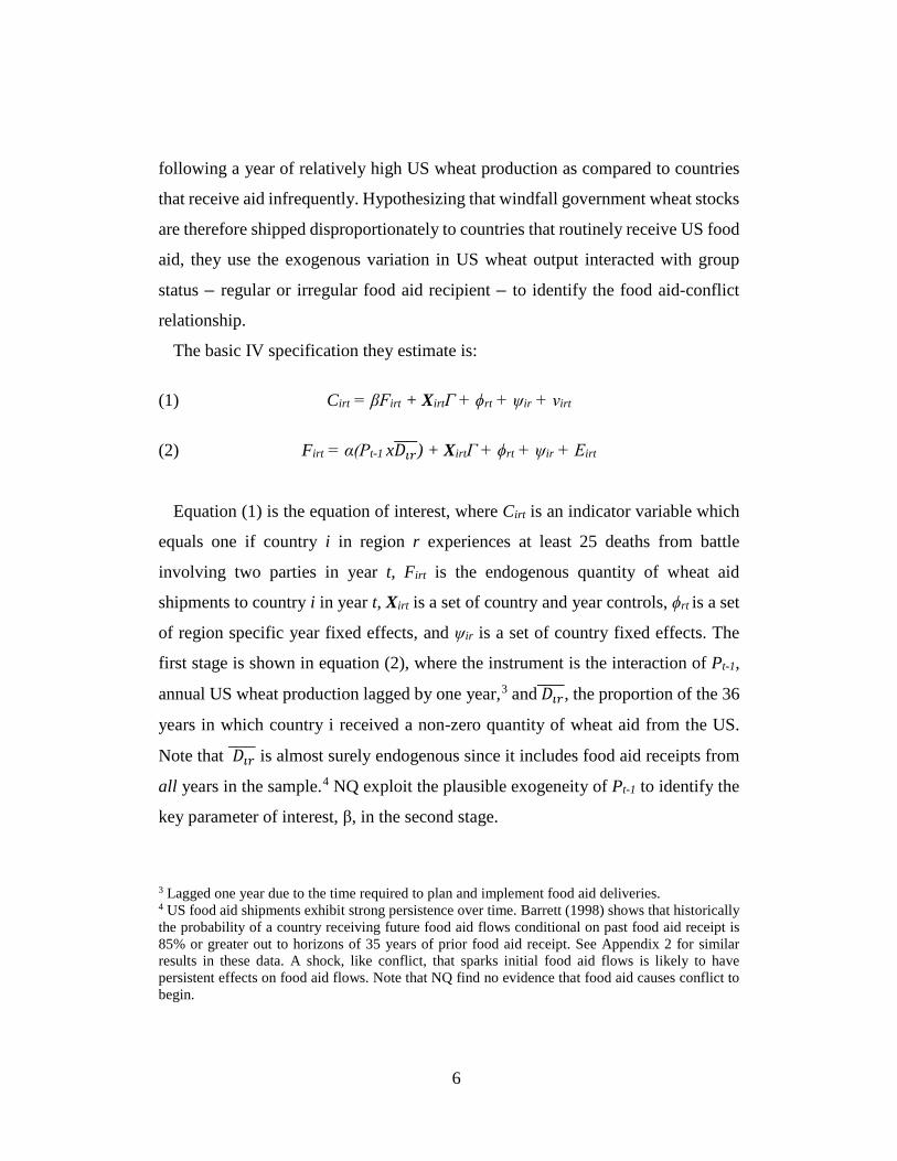
The basic IV specification they estimate is:

(1) Cirt = βFirt + XirtΓ + ϕrt + ψir + νirt

(2) Firt = α(Pt-1 x𝐷𝐷𝚤𝚤𝚤𝚤����) + XirtΓ + ϕrt + ψir + Εirt

Equation (1) is the equation of interest, where Cirt is an indicator variable which

equals one if country i in region r experiences at least 25 deaths from battle

involving two parties in year t, Firt is the endogenous quantity of wheat aid

shipments to country i in year t, Xirt is a set of country and year controls, ϕrt is a set

of region specific year fixed effects, and ψir is a set of country fixed effects. The

first stage is shown in equation (2), where the instrument is the interaction of Pt-1,

annual US wheat production lagged by one year,3 and 𝐷𝐷𝚤𝚤𝚤𝚤�����, the proportion of the 36

years in which country i received a non-zero quantity of wheat aid from the US.

Note that 𝐷𝐷𝚤𝚤𝚤𝚤����� is almost surely endogenous since it includes food aid receipts from

all years in the sample.4 NQ exploit the plausible exogeneity of Pt-1 to identify the

key parameter of interest, β, in the second stage.

3 Lagged one year due to the time required to plan and implement food aid deliveries. 4 US food aid shipments exhibit strong persistence over time. Barrett (1998) shows that historically the probability of a country receiving future food aid flows conditional on past food aid receipt is 85% or greater out to horizons of 35 years of prior food aid receipt. See Appendix 2 for similar results in these data. A shock, like conflict, that sparks initial food aid flows is likely to have persistent effects on food aid flows. Note that NQ find no evidence that food aid causes conflict to begin.

7

The justification for this first stage is that when additional wheat is available

because of high production (Pt-1), additional aid is sent to regular food aid

recipients, which goes disproportionately to the favored aid partners. Including the

country and year fixed effects, α is then analogous to a difference-in-difference

(DID) coefficient estimate, where the variation in the instrument comes from

comparing aid between high and low wheat production years and between regular

and irregular aid recipients. Any confounding variables that have a common effect

on conflict across all countries within a region in the same year, such as weather or

climate or global market prices, or characteristics of countries that have a constant

effect on conflict prevalence over time are controlled for through region-year and

country fixed effects.

In their preferred specification, NQ estimate equation (1) via 2SLS with the

interacted instrument in first stage equation (2) used for endogenous aid quantity,

and find that “a 1,000 MT increase in US wheat aid increases the incidence of

conflict by .3 percentage points.” At the sample means, their estimated food aid

elasticity of conflict incidence is 0.4, a large enough magnitude to warrant serious

policy attention.

But NQ’s conclusions depend on the credibility of the exclusion restriction

behind their IV strategy, which is that US wheat production conditional on the set

of controls reported in the paper is correlated with conflict only through the

following channel. Positive shocks from higher wheat production year-on-year lead

the US government to purchase more wheat in order to maintain a target price for

wheat, which loosens the budget constraints for aid agencies and allows them to

distribute more wheat aid the following year. The extra aid sent as a result causes

conflict prevalence to increase.5

5 The exact channel by which this last stage occurs is not clear. NQ argue that the extra food aid is vulnerable to theft, which allows rebels to continue fighting longer than they otherwise would. But this seems to contradict findings in the literature that show that exogenous sources of income growth

8

We show below that including year fixed effects does not eliminate the influence

of seemingly spurious correlation between wheat production and conflict because

both variables display a similar inverted-U shape trend over the period, and,

crucially, this trend is much more pronounced for regular aid recipients than for

irregular ones. This is akin to violating the parallel trends assumption essential to

identification in DID estimation; the differences are that in the NQ context – and in

other recent papers that use a similar technique – the trends are nonlinear and the

exposure variable is continuous, not binary. Including region-year and country

fixed effects, even a time trend variable, does not permit causal identification unless

either (i) the controls employed by NQ absorb all of the trend effects other than aid,

or (ii) inter-annual US wheat production fluctuations and resulting food aid are in

fact the dominant sources of the conflict trends.

These assumptions are much stronger than those described by NQ as the

necessary and sufficient conditions for their strategy to reveal a causal effect of aid

on conflict. Because the causal effect of aid on conflict is a relationship of

substantial interest to policy makers, and because the clever econometric trick they

employ appears in other empirical papers on other topics, we deem it important to

highlight the caveats to the NQ conclusions and to demonstrate their vulnerability

to spurious correlation due to nonlinear heterogeneous trends unrelated to the

hypothesized mechanism. Indeed, we can go further and show, via Monte Carlo

estimation, that a data generating process directly contrary to their hypothesized

causal mechanism generates remarkably similar parameter estimates in the

presence of the sorts of trends found in their data. A data system in which food aid

reduces rather than exacerbates conflict incidence produces the NQ results if trends

in wheat production and conflict are non-linear across countries and years.

are often associated with lower conflict (Blattman and Miguel, 2010). The mechanisms that would explain why income from aid deliveries would be more likely to be stolen by rebels and increase conflict while income from other sources often reduces fighting have not been established.

9

Understanding the sources of spurious and endogenous correlation between the

instrument and the outcome variable sheds important light on cautions to take when

implementing a similar IV strategy in panel data.

II. Placebo Test Failures

We begin the analysis of the 2SLS strategy by showing how policy changes over

the period can demonstrate the risk of misidentification. The mechanism driving

variation in the NQ setup is the assertion that US wheat price stabilization policies

oblige the USDA to purchase food in high production years. NQ argue that this

extra wheat aid is mostly sent to the countries that are the most regular recipients

of wheat aid from the US, and exploit the resulting difference in additional

allocations between high and low US wheat production years across regular and

irregular recipients of aid to try to identify a causal effect of food aid on conflict in

recipient countries.

Two fundamental problems exist, however. First, the connection between US

wheat production and USDA purchases is highly stylized, neglecting dramatic

changes in US farm support and food aid procurement policies during the study

period (Barrett and Maxwell, 2005). Most notably, the wheat price support policies

that are the exogenous mechanism linking wheat production to food aid shipments

changed, starting with the 1985 Farm Bill and culminating in the 1996 Farm Bill

which formally uncoupled government purchases from price or production targets

(Willis and O’Brien, 2015).6,7 This policy change implies that NQ’s hypothesized

6 The details of the policy and how it affects the estimation strategy are described in more detail in Appendix 1, which also explains why the mechanism NQ posit is largely irrelevant today, given changes in both US farm and food aid policies.

7 Following the 1996 Farm Bill, the USDA was still enabled, though not obligated, to purchase wheat through the Commodities Credit Corporation (CCC). It is possible that wheat yields would remain associated with price or supply changes that could differentially create incentives to purchase

10

first stage relationship between US wheat production and food aid deliveries should

be strongest prior to 1985 and should disappear or at least attenuate after 1996.

Thus, the latter portion of the NQ data offer a natural placebo test as the

mechanism tapered off after that point. When we re-estimate for sub-samples

before 1985, from 1985-1996, and after the wheat price stabilization policy ended

in 1996, however, rather than finding the hypothesized positive first and second

stage relationship in the pre-1985 period and no correlation in the latter period, we

find a positive association both between aid deliveries and wheat production (first

stage) and between conflict and aid as instrumented by wheat production (IV result)

in both the early (pre-1985) and latter (post-1996) periods, as reflected in Appendix

1.8 The results from the pre-1985 period where the posited policy mechanism was

indeed active are statistically indistinguishable from those from the post-1996

period when it no longer existed. And the estimated relationship during the policy

change period of 1985-1996 is negative, not positive, and statistically insignificant,

inconsistent with the NQ interpretation that aid causes conflict. Although it is

possible that discretionary purchases in the post-1996 period exactly mirrored the

pre-1985 period when purchases under certain market conditions were mandated,

the channel for the link between wheat production and aid shipments would be

much more speculative and open to concerns that the channel was associated with

potentially omitted variables such as price changes or supply shocks. This placebo

test suggests that something other than the hypothesized causal mechanism

wheat for aid under the Bill Emerson Humanitarian Trust or 416(b) programs in years with elevated wheat production, rather than draw on government-held stocks. However, such episodes have been relatively infrequent and when they have occurred, the bulk of the wheat procured has been used primarily for non-emergency Title II shipments that are monetized by the recipient NGO, i.e., not in emergency situations where food aid might prolong a conflict, as NQ hypothesize.

8 Except where additional data sources are added and explicitly noted, we use the dataset posted by Nunn and Qian on the replication files page at: https://www.aeaweb.org/articles?id=10.1257/aer.104.6.1630. These data are described in further detail in the original NQ paper. Where relevant, we refer to these data as the NQ replication file.

11

identified by the mandates of pre-1985 US farm policy might drive the correlation

NQ document between food aid flows and conflict.

Given the concerns raised by the policy robustness checks, we show through a

more general approach that NQ’s identification strategy is susceptible to a

particular and previously unappreciated problem that can arise when using an

interacted variable as an instrument in panel data. Intuitively, the first stage of the

IV strategy is a form of DID estimator. If the standard parallel trends assumption

in DID is violated, the exclusion restriction underpinning the IV approach fails.

In the NQ context, the problem arises because one component of the interacted

instrument is a time series variable (US wheat production) that is constant across

recipient country observations within the same year. The other component

(propensity to receive US food aid) varies only across cross-sectional observations,

not over years, and is likely to be endogenous to the outcome of interest (conflict

incidence), since food aid response to complex humanitarian emergencies

involving conflict is a central part of the main food aid program’s mission. On

closer inspection, we find that the time series variable exhibits strong nonlinear

trends strikingly similar to those observed in the outcome variable of interest in the

more exposed group of countries but not in the less exposed group, and that most

of the variation in the temporal component of the instrument comes from long term

trends rather than from year-on-year short term variation around the trend. Because

of the inter-group differences in the long-run nonlinear trend in the outcome

variable, the plausibly exogenous inter-annual variation in US wheat production are

likely not identifying the correlation between the IV and the dependent variable;

rather the differential underlying trends are.

Appendix 2 presents a detailed analysis of these heterogeneous nonlinear trends

along the (potentially endogenous) regular-irregular aid recipient dimension NQ

use for identification. This is problematic because NQ construct an instrument that

interacts the exogenous time series variable and the endogenous cross-sectional

12

variable, attempting to control for endogeneity through region-year and country

fixed effects, and in some specifications with linear time trends. The problem is

that inclusion of region-year and country fixed effects or a linear time trend does

not preclude the possibility that an observed relationship between the

(instrumented) endogenous variable and the outcome variable arises from spurious

correlation from dominant nonlinear trends.

In the NQ setting, wheat production and conflict both show strong trends over

time that swamp the more plausibly exogenous year-to-year variation. The trend in

conflict propensity is most apparent for countries that receive aid most often and

weakest for countries that do not receive aid frequently, meaning that including

year fixed effects as controls does not eliminate this source of endogeneity.

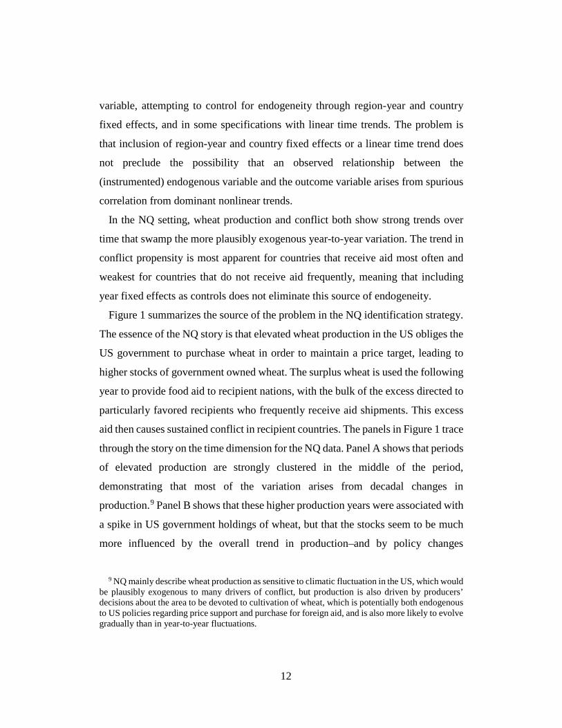
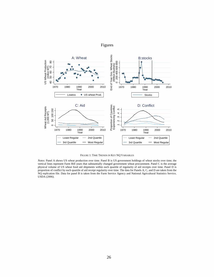
Figure 1 summarizes the source of the problem in the NQ identification strategy.

The essence of the NQ story is that elevated wheat production in the US obliges the

US government to purchase wheat in order to maintain a price target, leading to

higher stocks of government owned wheat. The surplus wheat is used the following

year to provide food aid to recipient nations, with the bulk of the excess directed to

particularly favored recipients who frequently receive aid shipments. This excess

aid then causes sustained conflict in recipient countries. The panels in Figure 1 trace

through the story on the time dimension for the NQ data. Panel A shows that periods

of elevated production are strongly clustered in the middle of the period,

demonstrating that most of the variation arises from decadal changes in

production.9 Panel B shows that these higher production years were associated with

a spike in US government holdings of wheat, but that the stocks seem to be much

more influenced by the overall trend in production–and by policy changes

9 NQ mainly describe wheat production as sensitive to climatic fluctuation in the US, which would

be plausibly exogenous to many drivers of conflict, but production is also driven by producers’ decisions about the area to be devoted to cultivation of wheat, which is potentially both endogenous to US policies regarding price support and purchase for foreign aid, and is also more likely to evolve gradually than in year-to-year fluctuations.

13

(described in Appendix 1)–than by year-to-year variation around the trend. Panel C

shows the trends in food aid receipt dividing by countries’ propensity to receive

aid; this variation is the key source of NQ’s identification. Almost all of the

variation comes from a powerful, approximately quadratic trend among only the

most frequent aid recipients. Finally, Panel D shows the trends in conflict among

categories of countries grouped by their frequency of US wheat aid receipt. Among

the most regular recipients of wheat aid, conflict prevalence shows a strong

inverted-U shape quite like that of wheat food aid shipments to that same group of

countries.

Together, these results indicate how spurious correlation could easily drive the

NQ results. The 1980s and 1990s were periods of elevated civil conflict. In the

same period, US wheat production happened to be high and the US had elevated

wheat aid shipments. Most of the wheat distributed as food aid in that period was

sent to countries experiencing conflict. These very broad trends reflect the variation

off of which NQ’s IV strategy identifies, but in no way does this identification

imply a causal connection between wheat shipments and aid. It is possible, as NQ

argue, that the trending wheat production caused aid shipments to be higher and

that these elevated aid shipments were responsible for the bulge in conflict shown

in this trend. But it seems at least as plausible that the relationship is entirely

spurious, driven by a simple coincidence of trends for three variables (wheat

production, total quantity of food aid shipments, and conflict) that evolve according

to highly autocorrelated nonlinear processes that happened to track each other over

the relatively short period NQ study, but differentially among regular and irregular

food aid recipients. Given that periods when wheat yields are elevated are clustered

together, the fact that conflict is high only in these periods does not force one to the

conclusion that aid is causing conflict. The fact that aid was mostly sent to the

countries that experienced conflict could just be a consequence of the fact that aid

14

is mostly shipped to places experiencing humanitarian disasters such as conflict,

exactly the simultaneity bias that the strategy is meant to circumvent.

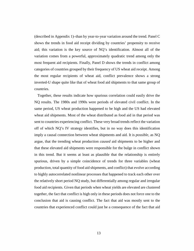
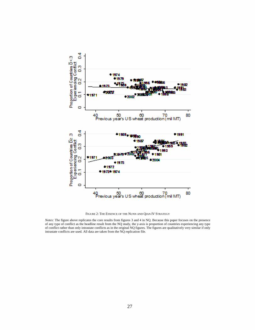
An intuitive way to show graphically how such time trends influence NQ’s IV

estimate is to reproduce the plots NQ use to explain and demonstrate their strategy,

highlighting changes across decades. Figure 2 reproduces the NQ’s Figures 3 and

4, which show the relationship between US wheat production and the proportion of

countries in each year who are experiencing a conflict. The bottom panel shows the

relationship among only the 50% of countries that receive aid from the US most

frequently, while the top panel is the 50% of countries that receive aid least

frequently during the study period. NQ use these plots to show that that wheat

production is related to conflict, but only among frequent recipients of US aid,

presenting an intuitively appealing demonstration for what is effectively the

reduced form in their IV strategy.

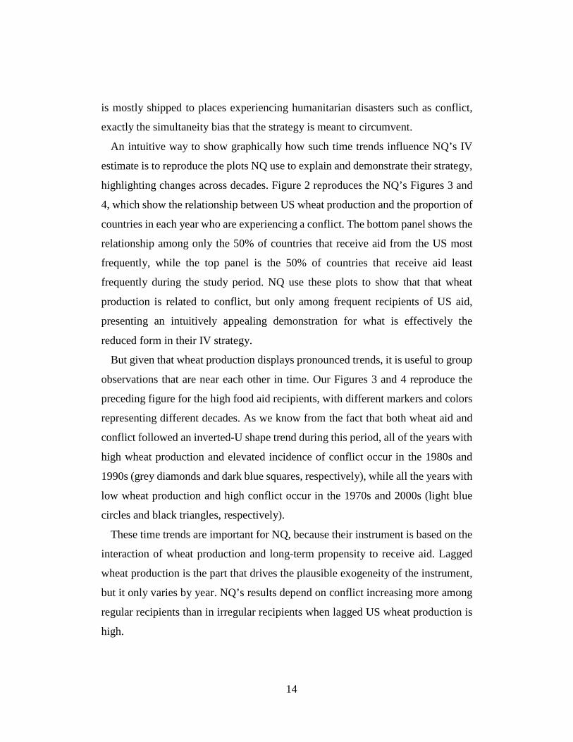
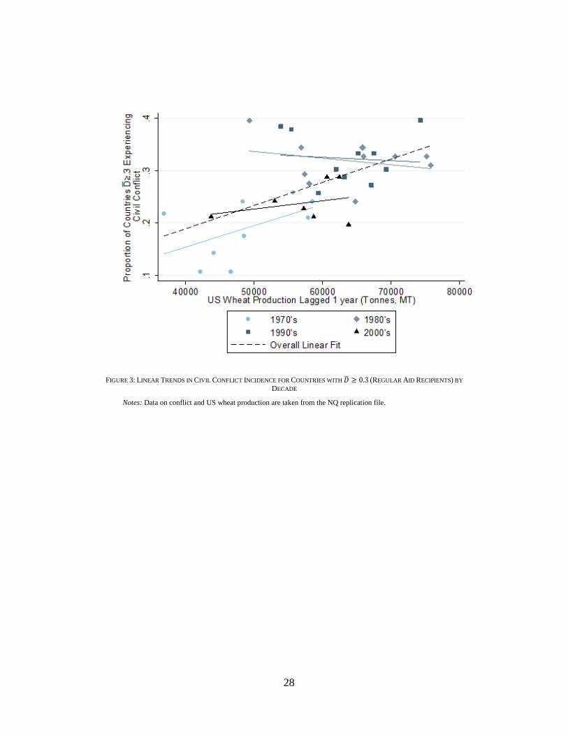
But given that wheat production displays pronounced trends, it is useful to group

observations that are near each other in time. Our Figures 3 and 4 reproduce the

preceding figure for the high food aid recipients, with different markers and colors

representing different decades. As we know from the fact that both wheat aid and

conflict followed an inverted-U shape trend during this period, all of the years with

high wheat production and elevated incidence of conflict occur in the 1980s and

1990s (grey diamonds and dark blue squares, respectively), while all the years with

low wheat production and high conflict occur in the 1970s and 2000s (light blue

circles and black triangles, respectively).

These time trends are important for NQ, because their instrument is based on the

interaction of wheat production and long-term propensity to receive aid. Lagged

wheat production is the part that drives the plausible exogeneity of the instrument,

but it only varies by year. NQ’s results depend on conflict increasing more among

regular recipients than in irregular recipients when lagged US wheat production is

high.

15

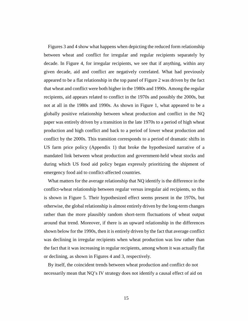
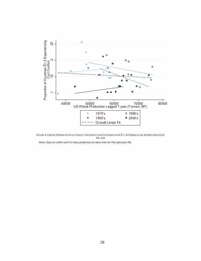
Figures 3 and 4 show what happens when depicting the reduced form relationship

between wheat and conflict for irregular and regular recipients separately by

decade. In Figure 4, for irregular recipients, we see that if anything, within any

given decade, aid and conflict are negatively correlated. What had previously

appeared to be a flat relationship in the top panel of Figure 2 was driven by the fact

that wheat and conflict were both higher in the 1980s and 1990s. Among the regular

recipients, aid appears related to conflict in the 1970s and possibly the 2000s, but

not at all in the 1980s and 1990s. As shown in Figure 1, what appeared to be a

globally positive relationship between wheat production and conflict in the NQ

paper was entirely driven by a transition in the late 1970s to a period of high wheat

production and high conflict and back to a period of lower wheat production and

conflict by the 2000s. This transition corresponds to a period of dramatic shifts in

US farm price policy (Appendix 1) that broke the hypothesized narrative of a

mandated link between wheat production and government-held wheat stocks and

during which US food aid policy began expressly prioritizing the shipment of

emergency food aid to conflict-affected countries.

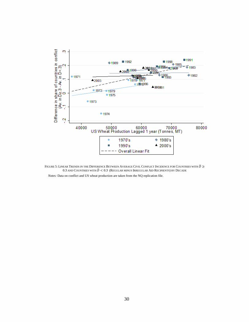
What matters for the average relationship that NQ identify is the difference in the

conflict-wheat relationship between regular versus irregular aid recipients, so this

is shown in Figure 5. Their hypothesized effect seems present in the 1970s, but

otherwise, the global relationship is almost entirely driven by the long-term changes

rather than the more plausibly random short-term fluctuations of wheat output

around that trend. Moreover, if there is an upward relationship in the differences

shown below for the 1990s, then it is entirely driven by the fact that average conflict

was declining in irregular recipients when wheat production was low rather than

the fact that it was increasing in regular recipients, among whom it was actually flat

or declining, as shown in Figures 4 and 3, respectively.

By itself, the coincident trends between wheat production and conflict do not

necessarily mean that NQ’s IV strategy does not identify a causal effect of aid on

16

conflict. Again, one interpretation of this correspondence is that higher wheat

production in the early 1980s and 1990s led the US government to procure greater

quantities of wheat, which was then shipped abroad as food aid, sustaining

conflict according the mechanisms proposed by NQ.

But since variation in wheat and conflict is mostly driven by long decadal

changes rather than year to year variation, there could well be omitted factors that

are related to both wheat production and conflict. It is entirely possible that the

evolution of two unrelated processes could coincide over time by coincidence.

Given that food aid is, by program design, intentionally directed toward countries

most at risk of conflict, such coincidence would generate spurious correlation and

bias in NQ’s IV estimates.

Depicting the variation over time in Figures 3 to 5 clearly shows how spurious

and endogenous variation could swamp more plausibly quasi-random variation

even with country and region-year fixed effects. To demonstrate the importance of

this effect we introduce a simple placebo test of whether the source of plausibly

exogenous inter-annual variation (US wheat production) on which the NQ strategy

relies – as do similar panel data IV strategies in other papers – indeed accounts for

the observed correlation. Our results strongly suggest that the NQ results are driven

by spurious correlation. Tests of this form should be widely applicable to similar

applications.

The placebo test we introduce is a form of randomization inference, and rests on

the simple principle that introducing randomness into the endogenous explanatory

variable of interest (a country’s food aid receipts in a given year) while holding

constant the (potentially endogenous) cross-sectional exposure variable ( 𝐷𝐷𝚤𝚤𝚤𝚤�����), the

instrument (US wheat production) and everything else should eliminate, or at least

substantially attenuate, the estimated causal relationship if indeed exogenous

inter-annual shocks to the endogenous explanatory variable (wheat food aid

shipments) drive outcomes (conflict in recipient countries). Within a given year,

17

we hold constant the following variables: the quantity of wheat produced, the

identity of the countries that receive any wheat food aid from the US (thereby

fixing both 𝐷𝐷𝚤𝚤𝚤𝚤����� and the timing of food aid receipts), observable fixed and time-

varying characteristics of countries, and the aggregate distribution of wheat food

aid allocations across all countries each year. But we randomly assign the key

variable of interest, the quantity of aid delivered to a particular country. For

example, in 1971, 60 countries received any wheat food aid from the US. In our

simulation, we randomly reassign (without replacement) the quantity of wheat aid

deliveries among these 60 countries, while holding constant the (true) zero value

of food aid receipts in the other countries. For example, instead of receiving the

2,100 tons it actually received in 1971, Nepal could be randomly assigned the 800

tons actually shipped to Swaziland that year. We similarly reshuffle the wheat aid

allocations among the 62 countries who received aid in 1972, and so on for every

year in the sample.

This new pseudo-dataset preserves the two sources of endogeneity we worry

about – time trends and endogenous selection into being a regular food aid

recipient –but sweeps out the source of variation that NQ have in mind by

randomizing among countries the assignment of specific food aid shipment

volumes. To keep with the earlier example, Swaziland’s food aid receipts cannot

plausibly have caused civil conflict within Nepal. This way, conflict can remain

spuriously related to wheat production because neither the conflict time series nor

the wheat production time series nor the exposure variable that distinguishes

between groups are altered, but the causal mechanism has been rendered non-

operational by randomization since it is no longer the case that in expectation

particular countries receive the randomly generated additional aid in a given year.

In this placebo test, the only reason why the quantity of wheat aid delivered

would be positively related to conflict in NQ’s baseline 2SLS specification would

be that countries that regularly experience conflict are also the countries that

18

regularly receive food aid (which is what we would expect if aid were targeted to

humanitarian crises) and the years of high wheat production happen to be years in

which conflict is elevated (which with only 36 years and strong trends could well

be spurious).

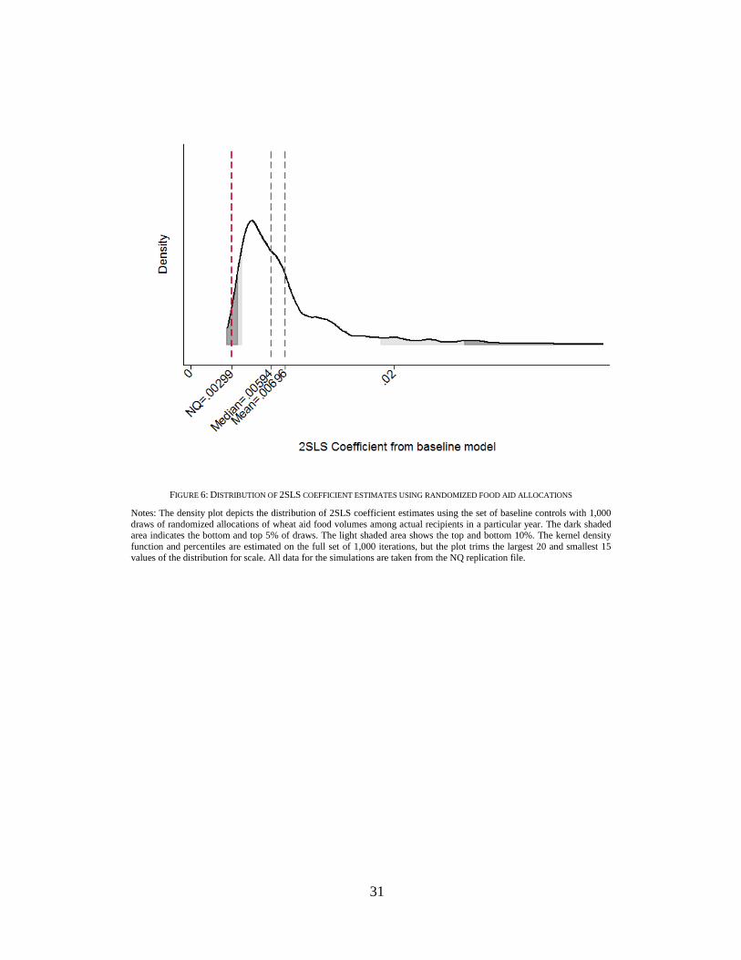
Figure 6 shows the distribution of coefficient estimates generated by 1,000

randomizations of food aid allocations and then (re-)estimating the baseline 2SLS

model. If the true causal relationship between food aid allocations and conflict

were positive and the identification was otherwise unaffected by selection bias

and spurious time trends, the distribution of coefficients would shift left relative

to the NQ coefficient estimate–and if the share of countries in which aid causes

conflict is small relative to a large enough sample, would center around zero–

because the randomization of food aid allocations would attenuate the estimated

relationship between aid and conflict. Instead, we find the opposite. The

distribution of parameter estimates clearly shifts to the right of the NQ 2SLS

coefficient estimate. This implies that the identity of aid recipient countries and

the overall trends in global conflict prevalence, US wheat production, and total

food aid deliveries drive the estimated relationship, not inter-annual fluctuations

in food aid receipts by a given country. Indeed, to the extent that the IV does

contain some component of random aid allocation, this test also signals that the

true association between inter-annual variation in food aid receipts and conflict

must be negative since eliminating that source of variation causes an increase in

coefficient estimates.

A third class of placebo test corroborates the confounding due to non-parallel

nonlinear trends. If spurious trends explain the NQ results, then any variable that is

elevated in the 1980s and 1990s relative to the 1970s and 2000s would correlate

spuriously with the outcome variable in the regular food aid recipient group, even

when keeping NQ’s instrument as a control. The placebo test is whether we can

replicate NQ’s findings using an obviously spurious instrument that follows the

19

same inverted U pattern over the sample period, even while controlling for their

instrument, just so as to ensure that the spurious instrument is not serving as a

coarse proxy for the true causal mechanism represented by the instrument.

Rejection of the null hypothesis that the spurious instrument has no effect indicates

failure of this placebo test. As detailed in Appendix 3, instrumenting for food aid

deliveries using a time series of global audio cassette tape sales, a clearly spurious

instrument chosen for its inverse-U time series over this period, rather than US

wheat production, generates remarkably similar IV results to NQ’s. When we

include NQ’s instrument as a control the point estimate is effectively zero while the

coefficient estimate on the spurious IV term in the second stage is statistically

insignificantly different from NQ’s original point estimate and significantly

different from zero. This test corroborates the hypothesis that their original

estimates are picking up long-run trends rather than the inter-annual variation that

underpins their hypothesized causal mechanism.

III. Monte Carlo Evidence

The preceding set of placebo tests call into question the causal interpretation NQ

give their IV estimates. To show that it is possible to replicate the NQ estimates

without the need to interpret their findings causally, we go one step further and

show that their results are in fact entirely consistent with a data generating process

in which either (i) food aid is statistically independent of conflict in recipient

countries or (ii) food aid receipts prevent conflict, the exact opposite of NQ’s causal

claim.

We use Monte Carlo simulations to show that NQ’s IV estimation method

generates parameter estimates similar to those NQ report, suggesting a positive,

causal effect of food aid on conflict, even when the true data generating process

(DGP) expressly has no such effect. The details of the constructed data generating

process and the simulation results are reported in Appendix 4.

20

The takeaway message is powerful. We can replicate the NQ results even if US

food aid agencies prefer to send food aid to conflict-affected countries–as is the

stated policy of the US food aid program (but opposite to how NQ explain the sign

shift between their OLS and 2SLS estimates) – and food aid has no causal effect

on–or even prevents (not prolongs) – civil conflict in recipient countries. The key

drivers of this result are (i) greater long-run variation than short-run variation in the

exogenous component of the instrument (US wheat production) and the outcome

variable (conflict), combined with (ii) spurious correlation in those longer-run

trends, as we demonstrate in Appendix 2.

This Monte Carlo exercise underscores that one needs to carefully explore the

longer-run time series patterns that might overwhelm the inter-annual variation

used to identify true causal effects, thereby generating spurious correlation in IV

panel data estimates. Because wheat production and conflict in regular aid

recipients both show pronounced, parallel trend patterns in the time series, but the

conflict incidence trend in irregular aid recipients does not parallel that of regular

aid recipients – and aid receipt is likely endogenous – NQ’s estimation strategy falls

prey to precisely this problem. This Monte Carlo result reinforces the conclusion

of the preceding placebo tests.

NQ recognize the possibility that trends could confound their inference. The

robustness checks NQ use, however, fail to identify the problematic relationships

in the model that drive these results. In Appendix 4, we show theirs to be a low

power test. This should serve as a cautionary tale to others attempting similar panel

data IV estimation strategies.

IV. Conclusions

This paper calls into question NQ’s empirical findings that US food aid shipments

cause conflict in recipient countries. We focus on the NQ results because they have

been widely publicized and inform an intensely debated policy issue that is

21

especially timely as the future of US foreign assistance and food aid in particular

under the next Farm Bill are under serious scrutiny. If a policy commonly labeled

“humanitarian” actually causes violent conflict, that policy should be revisited. We

show through a series of placebo tests that their results appear to result from longer-

run, spurious trends and then use Monte Carlo simulation to demonstrate that their

results could actually arise from a data generating process in which food aid is

independent of or even reduces conflict, contrary to their core claims that it

prolongs and thereby increases the incidence of conflict.

The broader methodological point, however, is that a panel data IV estimation

strategy that has become popular among researchers may be subject to heretofore

unrecognized inferential errors. An instrumental variable constructed as the

interaction of two variables, one that plausibly meets the exclusion restriction but

has limited time series variation, and another that has greater cross-sectional

variation in the sample but may be endogenous generates a continuous DID

estimator that is subject to the same parallel trends assumption as any other DID

estimator. In the presence of nonlinear non-parallel trends, standard fixed effects

controls may not suffice to isolate the exogenous inter-annual variability that is

intended to identify the causal effect of interest. Much like Bazzi and Clemens

(2013), we offer a caution about instrument validity and strength in panel data IV

estimation, and like Bertrand et al. (2004), we offer a caution about inference based

on DID methods.

The results reported by NQ have also been disputed by USAID (2014), who

report on robustness of the NQ strategy to controlling for other forms of non-food

aid external support for actors in civil conflicts including use of external military

bases and economic support for rebels. USAID suggests that when these variables

are included as controls, the statistical significance of food aid disappears.

Unfortunately, the USAID results are not directly comparable to the NQ strategy

for two reasons. First, external support to combatants only occurs by definition

22

when a conflict exists. Food aid, on the other hand is sent to both countries that are

experiencing conflict and those that are not, so that the NQ dataset can leverage

information from countries that are not actively experiencing conflict. Second, the

external aid variable is not available for the earliest years of NQ’s dataset. If NQ

identify a causal effect that is strongest in the early period, the USAID strategy

would miss the effect from those years. USAID argues that the NQ results are

fragile with regard to these robustness checks, but they are not able to fully explain

why the NQ strategy identifies an effect of aid on conflict. The threat to

identification we outline can explain both why NQ found an effect and why USAID

did not find an effect in their robustness checks. In addition to explaining why the

effects appear in the NQ data, our approach provides a template of checks that can

be used to assess the validity of similar approaches.

The best remedies for this prospective confounding are three. First, prudence

dictates acknowledging that one can only confidently identify associations, not

causal effects, as Peri (2012) does using this method. Second, try to identify

credible instruments also for the endogenous exposure variable, following Dube

and Vargas (2013). Third, carefully explore the patterns in the time series under

study. For example, Hanna and Oliva (2015) use the timing of the closing of a

refinery (which is plausibly exogenous but has limited variation) interacted with

the (endogenous) location of worker residence relative to the facility to identify the

effect of pollution exposure on labor supply. They present graphically the trends in

outcomes, which allows the reader to visually assess whether pre-existing trends

are likely to create spurious correlation to drive their results, a practice we applaud.

We recommend that authors using panel data IV strategies similar to NQ

explicitly investigate and report on trends in their instruments and outcome

variables to assess whether non-parallel trends could drive spurious results. The

simple randomization inference exercise we introduce, randomly resampling

without replacement the variable that generates the identifying source of variation,

23

while holding constant the trends meant to be controlled by fixed effects, may offer

a useful placebo test of similar identification strategies as a means to test whether

spurious trends rather than exogenous inter-annual variation are the true source of

statistical identification in the panel data.

24

REFERENCES

Barrett, Christopher B. (1998). “Food Aid: Is It Development Assistance, Trade

Promotion, Both or Neither?” American Journal of Agricultural Economics

80(3): 566-571.

Barrett, Christopher B. and Daniel G. Maxwell (2005). Food Aid After Fifty Years:

Recasting Its Role. New York: Routledge.

Bazzi, Samuel and Michael A. Clemens (2013). “Blunt Instruments: Avoiding

Common Pitfalls in Identifying the Causes of Economic Growth.” American

Economic Journal: Macroeconomics 5(2): 152-186.

Bertrand, Marianne, Esther Duflo, and Sendhil Mullainathan (2014). "How much

should we trust differences-in-differences estimates?" Quarterly Journal of

Economics 119(1): 249-275.

Chu, Chi-Yang, Daniel J. Henderson, and Le Wang (2016). “The Robust

Relationship Between US Food Aid and Civil Conflict.” Journal of Applied

Econometrics http://dx.doi.org/10.1002/jae.2558.

Dube, Oeindrila, and Juan F. Vargas (2013). "Commodity price shocks and civil

conflict: Evidence from Colombia." Review of Economic Studies 80(4): 1384-

1421.

Farm Service Agency and National Agricultural Statistics Service, USDA (2006).

“Appendix table 9--Wheat: Farm prices, support prices, and ending stocks,

1955/56-2005/06.” Accessed 14 May 2015.

www.ers.usda.gov/webdocs/DataFiles/

Hanna, Rema and Paulina Oliva (2015), “The Effect of Pollution on Labor Supply:

Evidence from a Natural Experiment in Mexico City.” Journal of Public

Economics 122 (1): 68–79.

Nunn, Nathan, and Nancy Qian (2014). “US Food Aid and Civil Conflict.”

American Economic Review 104(6): 1630-66.

25

Peri, Giovanni (2012). “The Effect of Immigration on Productivity: Evidence from

U.S. States.” Review of Economics and Statistics 94(1): 348–358.

USAID (2014). “(Re)Assessing The Relationship Between Food Aid and Armed

Conflict.” USAID Technical Brief.

Willis, Brandon and Doug O’Brien. “Summary and Evolution of U.S. Farm Bill

Commodity Titles.” National Agriculture Law Center. Accessed 26 January

2015. http://nationalaglawcenter.org/farmbills/commodity/

26

Figures

FIGURE 1: TIME TRENDS IN KEY NQ VARIABLES

Notes: Panel A shows US wheat production over time. Panel B is US government holdings of wheat stocks over time; the vertical lines represent Farm Bill years that substantially changed government wheat procurement. Panel C is the average physical volume of US wheat food aid shipments within each quartile of regularity of aid receipts over time. Panel D is proportion of conflict by each quartile of aid receipt regularity over time. The data for Panels A, C, and D are taken from the NQ replication file. Data for panel B is taken from the Farm Service Agency and National Agricultural Statistics Service, USDA (2006).

4050

6070

80

US

Whe

at P

rodu

ctio

n(m

illon

MT)

1970 1980 1990 2000 2010Year

Lowess US wheat Prod.

A: Wheat

020

040

060

080

0

End

of Y

ear G

ov. W

heat

Sto

cks

(Milli

on B

ushe

ls)

1970 1980 1990 2000 2010Year

Stocks

B:stocks

050

100

150

Whe

at A

id R

ecei

pts

(1,0

00 M

T)

1970 1980 1990 2000 2010Year

Least Regular 2nd Quartile

3rd Quartile Most Regular

C: Aid

.1.2

.3.4

.5

Prop

ortio

n of

Cou

ntrie

sEx

perie

ncin

g C

onfli

ct

1970 1980 1990 2000 2010Year

Least Regular 2nd Quartile

3rd Quartile Most Regular

D: Conflict

27

FIGURE 2: THE ESSENCE OF THE NUNN AND QIAN IV STRATEGY

Notes: The figure above replicates the core results from figures 3 and 4 in NQ. Because this paper focuses on the presence of any type of conflict as the headline result from the NQ study, the y-axis is proportion of countries experiencing any type of conflict rather than only intrastate conflicts as in the original NQ figures. The figures are qualitatively very similar if only intrastate conflicts are used. All data are taken from the NQ replication file.

28

FIGURE 3: LINEAR TRENDS IN CIVIL CONFLICT INCIDENCE FOR COUNTRIES WITH 𝐷𝐷� ≥ 0.3 (REGULAR AID RECIPIENTS) BY

DECADE

Notes: Data on conflict and US wheat production are taken from the NQ replication file.

29

FIGURE 4: LINEAR TRENDS IN CIVIL CONFLICT INCIDENCE FOR COUNTRIES WITH 𝐷𝐷� < 0.3 (IRREGULAR AID RECIPIENTS) BY

DECADE Notes: Data on conflict and US wheat production are taken from the NQ replication file.

30

FIGURE 5: LINEAR TRENDS IN THE DIFFERENCE BETWEEN AVERAGE CIVIL CONFLICT INCIDENCE FOR COUNTRIES WITH 𝐷𝐷� ≥

0.3 AND COUNTRIES WITH 𝐷𝐷� < 0.3 (REGULAR MINUS IRREGULAR AID RECIPIENTS) BY DECADE Notes: Data on conflict and US wheat production are taken from the NQ replication file.

31

FIGURE 6: DISTRIBUTION OF 2SLS COEFFICIENT ESTIMATES USING RANDOMIZED FOOD AID ALLOCATIONS

Notes: The density plot depicts the distribution of 2SLS coefficient estimates using the set of baseline controls with 1,000 draws of randomized allocations of wheat aid food volumes among actual recipients in a particular year. The dark shaded area indicates the bottom and top 5% of draws. The light shaded area shows the top and bottom 10%. The kernel density function and percentiles are estimated on the full set of 1,000 iterations, but the plot trims the largest 20 and smallest 15 values of the distribution for scale. All data for the simulations are taken from the NQ replication file.

32

FOR ONLINE PUBLICATION ONLY

Appendix 1: Further Details on US Farm Price Support and Food Aid

Policy Evolution

US commodity price stabilization and food aid policies experienced dramatic

changes during the period Nathan Nunn and Nancy Qian (2014, hereafter NQ)

study. We demonstrate that results of the NQ strategy do not correspond to the

periods in which the true policy regime was closest to the one they describe,

indicating that a source of variation other than US commodity price stabilization

and associated food aid policy is likely driving their results. Furthermore, the type

of policy regime they have in mind effectively ended in the mid-1990s, calling into

question the current policy relevance of their results given dramatic changes in the

way aid is distributed in recent decades.

A. Changes in Commodity Price Support and Surplus Disposal Policies

The mechanism NQ describe to generate the relationship between wheat

production and quantity of aid is the following: “The USDA accumulates wheat in

high production years as part of its price stabilization policies. The accumulated

wheat is stored and then shipped as food aid to poor countries.” The US long had a

policy of agricultural commodity price supports that indeed created a link between

aggregate annual production and government procurement of wheat that was

subsequently used as food aid; indeed, surplus disposal was an explicit policy

objective of the main US food aid program launched in 1954 (Barrett and Maxwell,

2005). However, US commodity price support and food aid procurement policies

changed dramatically during the period of the NQ data, and the true form of policy

has an important bearing on the interpretation of NQ’s IV strategy.

33

In practice, policies that link production to US government procurement were not

in place for the entire duration of the NQ study period. In the 1970s and early 1980s,

the start of the NQ time series, purchases took place through USDA’s system of

non-recourse loans, which were essentially loans that the USDA made to US

farmers through the USDA’s Commodity Credit Corporation (CCC).10 The USDA

would purchase a farmer’s grain production at a fixed rate if the market price fell

below that rate. In order to avoid having these large reserves putting downward

pressure on future grain prices, the USDA donated commodity stocks to countries

beyond its commercial marketshed as food aid through Section 416(b) of the

Agricultural Act of 1949, and subsequently through the food aid programs

authorized under Public Law 480 (PL480), passed in 1954, which became the

principal vehicle for US food aid shipments. Section 416(b) and PL480 shipments

driven by surplus disposal objectives thus became the primary connection between

food aid and civil conflict (Barrett and Maxwell, 2005; Schnepf, 2014). In this

system, USDA wheat purchases (i.e., grain forfeitures for nonpayment of non-

recourse commodity loans) were a function not only of the price, but also of the

underlying loan rates. However, the only period during the NQ study window when

loan rates fluctuated around market prices was a brief window between 1981 and

1986 (Westcott and Hoffman, 1999). This led government stocks of wheat to climb

sharply, with government stocks reaching 62% of average annual wheat production

1981-1987 (Wescott and Hoffman, 1999). This represented a peak for government

intervention in wheat markets, sparking changes to federal farm price support

programs in the mid-1980s.

10 A farmer could take out a non-recourse commodity loan proportionate to his or her harvested quantity of wheat at a

fixed unit rate with the grain held as collateral. Within a nine-month window, if the selling price of grain dipped below the loan repayment rate, the farmer could forfeit the grain rather than repay the loan. Effectively, this guaranteed the farmer the minimum of the rate fixed by CCC or the world price, and caused the CCC to purchase wheat when market prices were low. Government procurement was therefore a function not only of production and prices, but also of the level at which CCC set the loan repayment rate, a policy variable subject to revision in various Farm Bills.

34

High levels of procurement during that period and the excessive stocks that

resulted led to market reforms that de-linked wheat production and US food aid

procurement, particularly following the Farm Bills in 1985 and 1990. Finally, the

1996 Farm Bill uncoupled the link between wheat production and government held

stocks for good (Willis and O’Brien, 2015). CCC stocks of wheat were fully

exhausted by 2006, and indeed, the Section 416(b) food aid program has been

inactive since 2007 because of the unavailability of CCC-owned grain stocks

(Schnepf, 2014). Since the 1990s, a majority of US food aid has been procured on

open market tenders by USDA (Barrett and Maxwell 2005).

These differences in how NQ describe the policy and the historical realities of

commodity price support and food aid policy are important for the NQ

identification strategy. Given that federal law began to unravel the link between

wheat prices (and therefore wheat production) and government commodity

procurement for use in food aid programs starting with the 1985 Food Bill and

severed it in the 1996 Food Bill, if the mechanism NQ posit indeed drove their

findings, then the first stage of NQ’s IV strategy should be strongest prior to 1985

and non-existent after 1996. That turns out not to be the case. The post-1996

estimation is a sort of placebo test since the causal mechanism did not exist during

that sub-sample.

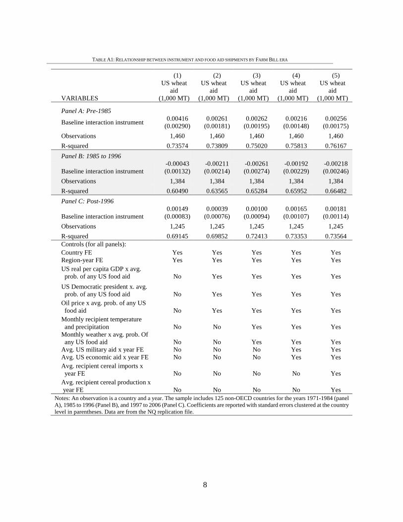
Table A1 implements this simple robustness check by reproducing the first stage

of the NQ strategy dividing the sample into three periods corresponding to the

passage of the Farm Bills that successively decoupled US wheat production from

government held wheat stocks. As expected, the connection between wheat

production and food aid shipments is strongest prior to 1985 but statistically

insignificant. In the years 1985 to 1996 the effect turns negative and statistically

insignificant, then is inexplicably similar to the NQ baseline result in the post 1996

period but still not statistically significant. The fact that we see a relationship

between wheat production and wheat food aid shipments after the US formally

35

ended the policy link that underpins NQ’s identification strategy suggests that the

first stage may be identifying spurious correlation not related to the claimed

exogenous mechanisms.

B. Changing Modalities and Priorities of US Food Aid

Given changes in procurement policies, the post-1996 relationship between

production and procurement is likely spurious, but it is possible that the NQ strategy

identifies a causal effect in the 1970-1985 period when US wheat production was

more closely linked to food aid shipments. But the question of whether the results

are driven by the period prior to 1985 is important, because US food aid policies

have changed dramatically over the period of NQ’s study in ways that are not taken

into account by the policy conclusions they offer based on their findings.

Food aid from the US is procured and distributed under multiple policies, each

with its own legal authorization, priorities, and processes. Both historically and

today, the bulk of food aid is distributed through PL480, which authorizes

procurement and distribution of aid by USDA, along with distribution of Title II of

PL480 by the US Agency for International Development (USAID) (Barrett and

Maxwell, 2005). But PL480 consists of several titles which describe very different

forms of aid.

Aid distributed by USDA through Title I of PL480 provides concessional sales

of food aid directly to foreign governments. Recipient governments have

historically sold off the vast majority of Title I food aid, treating these more as

balance of payments transfers in kind than as food for direct distribution. Title I aid

constituted the majority of food aid in the early period of NQ’s study, accounting

for 63% of US international Food Assistance Outlays between 1970 and 1979

(Schnepf, 2014). But the role of this direct-to-government concessional aid

36

declined precipitously over the period and no allocations at all have occurred under

Title I since 2006.

In contrast to Title I the role of aid distributed through Title II of PL480 has

increased dramatically. Title II permits USAID to allocate aid in response to

humanitarian emergencies and non-emergency food insecurity as an outright grant.

Unlike Tittle I, the vast majority of Title II food aid shipments are directly

distributed to food consumers; today only the statutory minimum of 15% of Title

II non-emergency shipments are sold (‘monetized’ in food aid jargon). Title II aid

is delivered through non-governmental organizations (NGOs) and private voluntary

organizations (PVOs) like CARE or CRS or through intergovernmental

organizations like the United Nations’ World Food Programme (WFP) rather than

directly to country governments. Title II accounted for less than 40% of US

international food assistance outlays in 1970-1979, but accounts for 88% of food

assistance today (Schnepf, 2014). If food aid distributed to governments is more

likely to fuel conflict (either because it is easier to steal or because governments

use the food to feed their own troops or the proceeds of food aid sales to finance

military operations) then it might be reasonable to expect that food aid in the 1970s

would be more likely to fuel conflict than food aid in more recent periods. But this

does not imply that the food aid distribution system that prevails today would have

this effect.

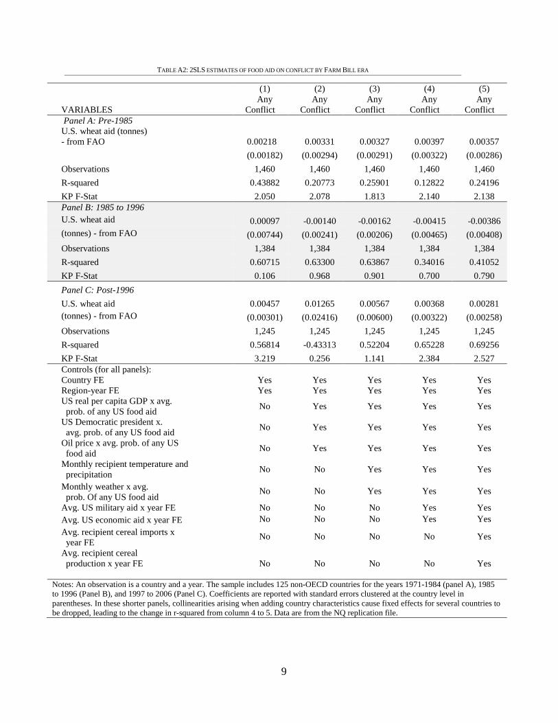
Table A2 reproduces NQ’s IV estimate of the relationship between food aid and

conflict, but splitting the sample by the same periods as in Table A1. Consistent

with the lack of a strong first stage relationship, we find no relationship between

aid and conflict in the period between the 1985 and 1996 Food Bills. As expected

given that the instrument is strongest in the pre-1985 period, the coefficients on aid

for this period are slightly bigger than those presented by NQ for the full sample.

In the post 1996 period, the coefficient is also very close to the one in the NQ paper.

The coefficient is not quite significant at standard levels, but given the smaller

37

number of observations in that period, we cannot reject the null hypothesis of

equivalence of the coefficients prior to 1985 and following 1996. Strikingly, despite

the fact that food aid was administered very differently in the 2000s than in the

1970s, the coefficients for these two periods are nearly identical. Thus, one is left

with two possible conclusions. Either, the delivery mechanisms behind food aid is

irrelevant to the degree to which food aid translates into elevated conflict – which

seems unlikely – or the NQ IV strategy is picking up something other than a causal

effect of aid on conflict.

C. Incompatibility of OLS Results with Stated Goals of Aid Agencies

An additional indication of a problem with interpreting NQ’s results is their

implausible claim that the modest, statistically insignificant negative association

between food aid and conflict in their OLS estimates suffers significant negative

bias. The NQ explanation for that claim is the possibility that donors condition food

aid flows on characteristics correlated with low levels of conflict, i.e., that the US

actively seeks to avoid sending foreign aid to conflict-affected countries. This

explanation directly contradicts USAID’s Food for Peace program’s stated

objective “FFP provides emergency food assistance to those affected by conflict

and natural disasters and provides development food assistance to address the

underlying causes of hunger.” (USAID, 2015, emphasis added) In the NQ dataset,

less than 22% of countries experience conflict in the average year, and yet between

1975 and 2006, there were only 2 years when there were more countries receiving

food aid and not experiencing conflict than countries who were both receiving food

aid and experiencing conflict.

As US food aid shifted from Title I lending to governments to Title II emergency

assistance through PVS/NGOs and WFP, food aid has grown increasingly

concentrated on populations dealing with conflict, contrary to the NQ hypothesis.

38

If food aid deliveries intentionally directed toward countries that have conflict

rather than away from such countries, reconciling a positive IV coefficient with a

negative OLS coefficient becomes difficult. If humanitarian assistance during

conflict is a primary source of endogeneity, one would have expected the OLS

coefficient to be upward biased rather than downward as would be implied by NQ’s

reported effects.

8

TABLE A1: RELATIONSHIP BETWEEN INSTRUMENT AND FOOD AID SHIPMENTS BY FARM BILL ERA

(1) (2) (3) (4) (5)

VARIABLES

US wheat aid

(1,000 MT)

US wheat aid

(1,000 MT)

US wheat aid

(1,000 MT)

US wheat aid

(1,000 MT)

US wheat aid

(1,000 MT)

Panel A: Pre-1985 Baseline interaction instrument 0.00416

(0.00290) 0.00261

(0.00181) 0.00262

(0.00195) 0.00216

(0.00148) 0.00256

(0.00175) Observations 1,460 1,460 1,460 1,460 1,460 R-squared 0.73574 0.73809 0.75020 0.75813 0.76167 Panel B: 1985 to 1996

Baseline interaction instrument -0.00043 (0.00132)

-0.00211 (0.00214)

-0.00261 (0.00274)

-0.00192 (0.00229)

-0.00218 (0.00246)

Observations 1,384 1,384 1,384 1,384 1,384 R-squared 0.60490 0.63565 0.65284 0.65952 0.66482 Panel C: Post-1996

Baseline interaction instrument 0.00149

(0.00083) 0.00039

(0.00076) 0.00100

(0.00094) 0.00165

(0.00107) 0.00181

(0.00114) Observations 1,245 1,245 1,245 1,245 1,245 R-squared 0.69145 0.69852 0.72413 0.73353 0.73564 Controls (for all panels): Country FE Yes Yes Yes Yes Yes Region-year FE Yes Yes Yes Yes Yes US real per capita GDP x avg. prob. of any US food aid No Yes Yes Yes Yes US Democratic president x. avg. prob. of any US food aid No Yes Yes Yes Yes Oil price x avg. prob. of any US food aid No Yes Yes Yes Yes Monthly recipient temperature and precipitation No No Yes Yes Yes Monthly weather x avg. prob. Of any US food aid No No Yes Yes Yes Avg. US military aid x year FE No No No Yes Yes Avg. US economic aid x year FE No No No Yes Yes Avg. recipient cereal imports x year FE No No No No Yes Avg. recipient cereal production x year FE No No No No Yes

Notes: An observation is a country and a year. The sample includes 125 non-OECD countries for the years 1971-1984 (panel A), 1985 to 1996 (Panel B), and 1997 to 2006 (Panel C). Coefficients are reported with standard errors clustered at the country level in parentheses. Data are from the NQ replication file.

9

TABLE A2: 2SLS ESTIMATES OF FOOD AID ON CONFLICT BY FARM BILL ERA

(1) (2) (3) (4) (5)

VARIABLES Any

Conflict Any

Conflict Any

Conflict Any

Conflict Any

Conflict Panel A: Pre-1985 U.S. wheat aid (tonnes) - from FAO

0.00218 0.00331 0.00327 0.00397 0.00357

(0.00182) (0.00294) (0.00291) (0.00322) (0.00286) Observations 1,460 1,460 1,460 1,460 1,460 R-squared 0.43882 0.20773 0.25901 0.12822 0.24196 KP F-Stat 2.050 2.078 1.813 2.140 2.138 Panel B: 1985 to 1996 U.S. wheat aid 0.00097 -0.00140 -0.00162 -0.00415 -0.00386 (tonnes) - from FAO (0.00744) (0.00241) (0.00206) (0.00465) (0.00408) Observations 1,384 1,384 1,384 1,384 1,384 R-squared 0.60715 0.63300 0.63867 0.34016 0.41052 KP F-Stat 0.106 0.968 0.901 0.700 0.790 Panel C: Post-1996 U.S. wheat aid 0.00457 0.01265 0.00567 0.00368 0.00281 (tonnes) - from FAO (0.00301) (0.02416) (0.00600) (0.00322) (0.00258) Observations 1,245 1,245 1,245 1,245 1,245 R-squared 0.56814 -0.43313 0.52204 0.65228 0.69256 KP F-Stat 3.219 0.256 1.141 2.384 2.527 Controls (for all panels): Country FE Yes Yes Yes Yes Yes Region-year FE Yes Yes Yes Yes Yes US real per capita GDP x avg. prob. of any US food aid No Yes Yes Yes Yes

US Democratic president x. avg. prob. of any US food aid No Yes Yes Yes Yes

Oil price x avg. prob. of any US food aid No Yes Yes Yes Yes

Monthly recipient temperature and precipitation No No Yes Yes Yes

Monthly weather x avg. prob. Of any US food aid

No No Yes Yes Yes

Avg. US military aid x year FE No No No Yes Yes Avg. US economic aid x year FE No No No Yes Yes Avg. recipient cereal imports x year FE

No No No No Yes

Avg. recipient cereal production x year FE

No No No No Yes

Notes: An observation is a country and a year. The sample includes 125 non-OECD countries for the years 1971-1984 (panel A), 1985 to 1996 (Panel B), and 1997 to 2006 (Panel C). Coefficients are reported with standard errors clustered at the country level in parentheses. In these shorter panels, collinearities arising when adding country characteristics cause fixed effects for several countries to be dropped, leading to the change in r-squared from column 4 to 5. Data are from the NQ replication file.

10

Appendix 2. Heterogeneous Time Trends in the Data

We now explore the secular time trends in the data and potential sources of the

coincident time trends in wheat production, food aid shipments, and conflict. In

Appendix 4 we use these findings to assess whether the controls included by NQ

can address the bias in their estimation results. If the trends are unrelated and due

only to spurious association due to persistence in the evolution of both variables,

then one can eliminate the bias only by knowing the exact structure of the process

driving the system. The linear fixed effects controls NQ employ are not sufficient.

We also explore whether the controls can eliminate the bias if the trends in conflict

are attributable only to the influence of a known and measurable variable that

follows a trend over the period. Using the example of variation in sea surface

temperature associated with El Niño Southern Oscillation (ENSO) events, we show

through additional simulations that controlling for the confounding variable after

the manner of NQ will only eliminate the bias if the relationship between the

confounding variable and conflict follows very particular patterns.

A. Global Time Trends in Key Variables

Figure 1, Panel A, shows US wheat production by year with a lowess plot

overlaid to show the underlying trend. Although there is substantial variation year

to year, a powerful nonlinear trend is also evident. US wheat production increased

rapidly between 1970 and the early 1980s. Wheat output then peaked in the middle

of the period, between 1981 and 1998, and then declined from the latter 1990s. A

pattern like this suggests that anything that was increasing in the 1970s, peaked

around 1990 and then declined, will be correlated with US wheat production,

whether spuriously or causally.

Food aid flows follow a very similar pattern. Figure A1 shows the trend average

US wheat food aid flows by year.

11

That food aid to particular countries is persistent has been well established in the

literature (Barrett, 1998; Jayne et al, 2002; Barrett and Heisey, 2002). Figure A2

demonstrates this persistence for wheat aid in the particular years and countries of

the NQ dataset by showing the distribution of aid spells by length, where a “spell”

is defined as a continuous stretch of years in which a country receives aid in each

year and spells are separated by those where there was a conflict in the country in

the first year of the spell and those where the country was not in conflict when the

spell began. Once aid starts, the country is likely to continue receiving aid for many

subsequent years. This is especially true if there is a conflict in the country when

the spell starts. This highlights the fact that aid allocations are highly endogenous;

once aid starts flowing to a country, it is likely to continue, and this is especially

true in conflict situations.

The degree of persistence has also changed over time as aid allocation priorities

have changed. Figure A3 shows the percentage of aid spells that last at least five

years by the year in which the spell started. Wheat aid was significantly more

persistent in the 1970s when most food aid flowed as (Title I PL480) annual

concessional exports to governments with established Title I programs. This

persistence lessened in the 1980s and 1990s as Title II grants to NGOs and WFP

began to replace Title I, catering to a different set of countries. The persistence grew

stronger again in the 2000s when USAID began concentrating non-emergency Title

II flows on just a few countries that routinely had emergency Title II flows for two

reasons: First, an aspiration that non-emergency might preempt some of the need

for emergency food aid flows, and, second, the administrative logistical advantages

in rapid emergency response that come from having non-emergency food aid

distribution pipelines in place and operational already when a disaster strikes or a

conflict erupts (Barrett and Maxwell, 2005).

Figure A4 shows a lowess plot of conflict incidence over the period in Nunn and

Qian’s study. On average, the incidence of conflict followed a similar trend to

12

wheat production, increasing in the early 1970s before peaking around 1990 and

declining for the rest of the period. Strikingly, the years in which the highest

proportion of countries experienced conflict seem to be the same as those in which

US wheat output was the highest and the years with the lowest wheat production

also had the lowest number of countries experiencing conflict. So, is this the causal

relation NQ claim or a spurious correlation? Given that NQ do not find any effect

on conflict onset, and that both aid and conflict are persistent, spurious correlation

seems the more likely explanation.

B. Differential Trends by Aid Recipients

Trends in the conflict and wheat production variables are not problematic for

NQ’s strategy if they are unrelated to the propensity to receive aid, since trends that

are common to all countries will be absorbed by the region-year fixed effects. A

simple way to check whether the trends vary by aid propensity is to graph conflict

by quartiles of aid receipt regularity, as shown in Figure 1, panel D. The darkest

line shows the trend for the quarter of countries which received aid in the greatest

percentage of years in the dataset. The lightest shaded line represents the countries

which receive aid in the lowest percentage of years. The most regular aid recipients

show a much stronger trend in conflict prevalence over the period, a trend that is

strikingly similar to that of US wheat production. As a result, NQ’s instrument will

pick up variation in conflict driven by this trend.

This does not differentiate trends by region, which is important, because Nunn

and Qian include interactions of the year dummies with dummies for six regions

used by the World Bank to group clusters of countries. If most of the difference in

conflict trends between regular and irregular aid recipient countries is driven by

differences in these regions, then NQ’s strategy would account for the differential

trends.

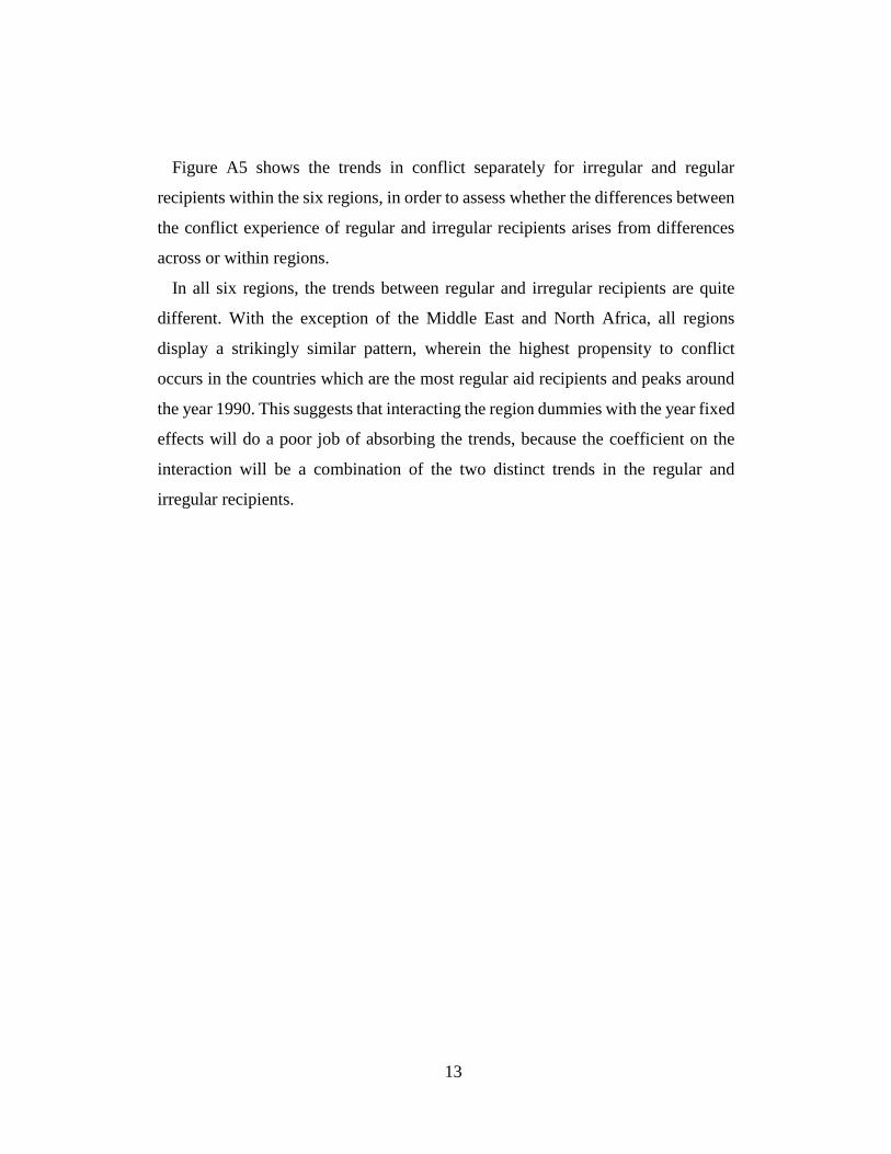
13

Figure A5 shows the trends in conflict separately for irregular and regular

recipients within the six regions, in order to assess whether the differences between

the conflict experience of regular and irregular recipients arises from differences

across or within regions.

In all six regions, the trends between regular and irregular recipients are quite

different. With the exception of the Middle East and North Africa, all regions

display a strikingly similar pattern, wherein the highest propensity to conflict

occurs in the countries which are the most regular aid recipients and peaks around

the year 1990. This suggests that interacting the region dummies with the year fixed

effects will do a poor job of absorbing the trends, because the coefficient on the

interaction will be a combination of the two distinct trends in the regular and

irregular recipients.

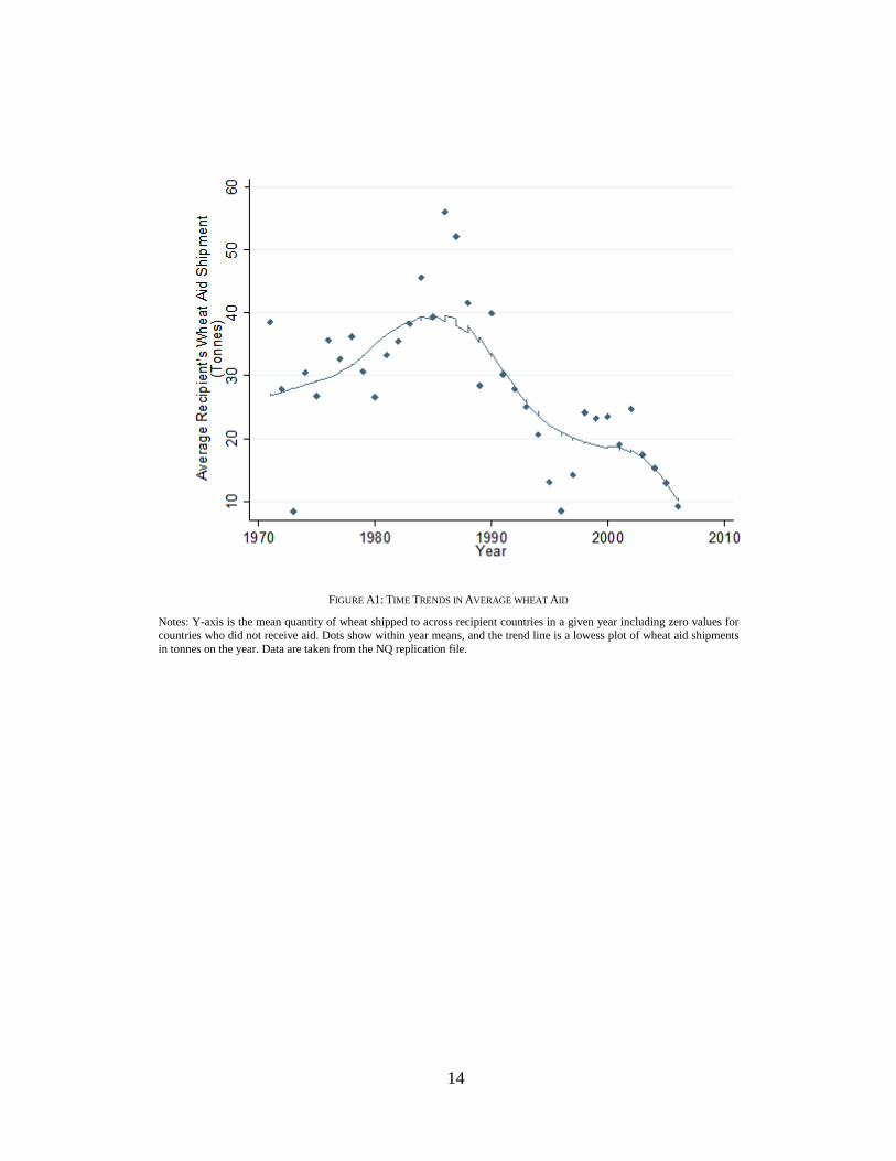
14

FIGURE A1: TIME TRENDS IN AVERAGE WHEAT AID

Notes: Y-axis is the mean quantity of wheat shipped to across recipient countries in a given year including zero values for countries who did not receive aid. Dots show within year means, and the trend line is a lowess plot of wheat aid shipments in tonnes on the year. Data are taken from the NQ replication file.

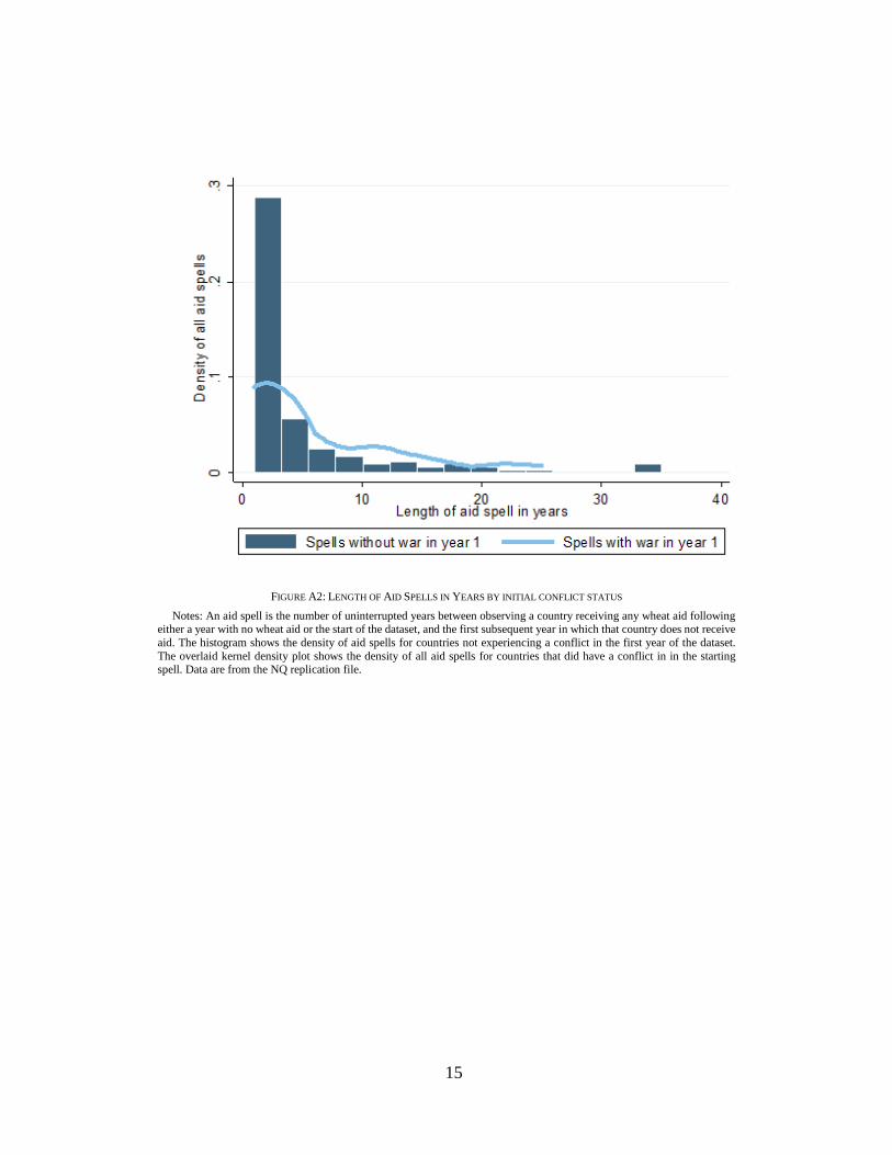
15

FIGURE A2: LENGTH OF AID SPELLS IN YEARS BY INITIAL CONFLICT STATUS

Notes: An aid spell is the number of uninterrupted years between observing a country receiving any wheat aid following either a year with no wheat aid or the start of the dataset, and the first subsequent year in which that country does not receive aid. The histogram shows the density of aid spells for countries not experiencing a conflict in the first year of the dataset. The overlaid kernel density plot shows the density of all aid spells for countries that did have a conflict in in the starting spell. Data are from the NQ replication file.

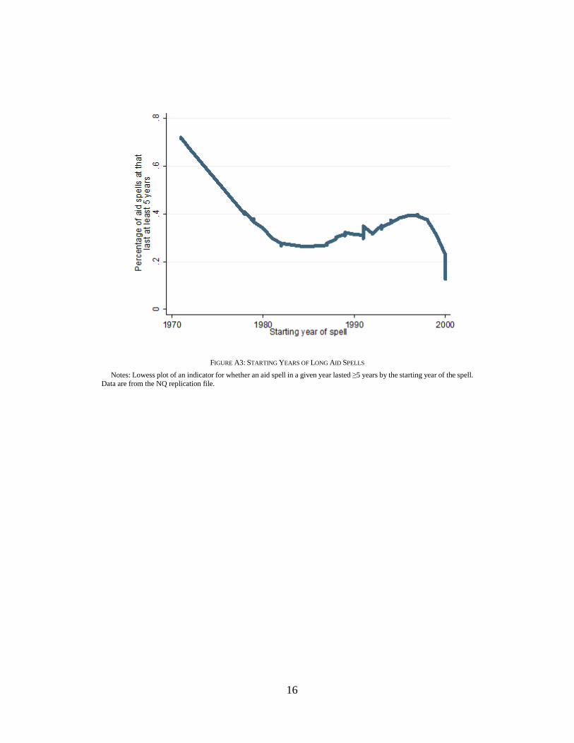
16

FIGURE A3: STARTING YEARS OF LONG AID SPELLS

Notes: Lowess plot of an indicator for whether an aid spell in a given year lasted ≥5 years by the starting year of the spell. Data are from the NQ replication file.

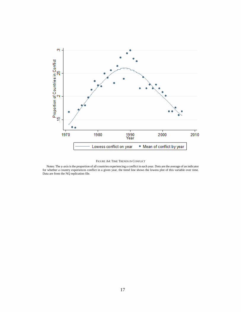
17

FIGURE A4: TIME TRENDS IN CONFLICT

Notes: The y-axis is the proportion of all countries experiencing a conflict in each year. Dots are the average of an indicator for whether a country experiences conflict in a given year, the trend line shows the lowess plot of this variable over time. Data are from the NQ replication file.

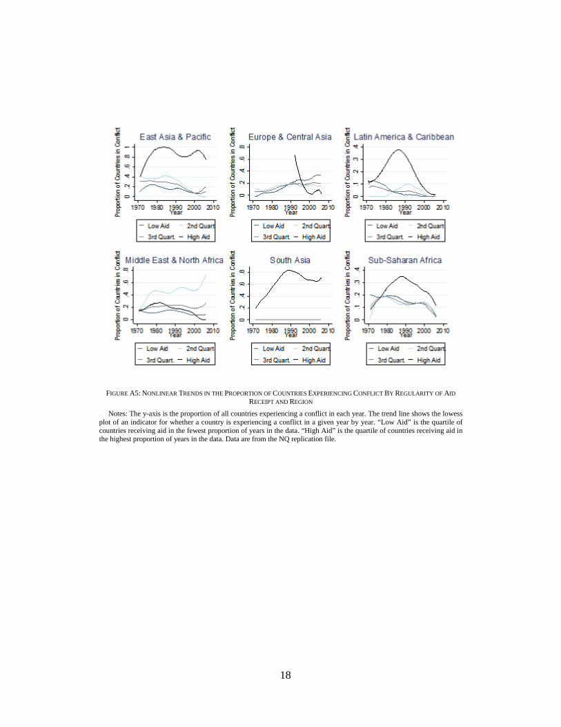
18

FIGURE A5: NONLINEAR TRENDS IN THE PROPORTION OF COUNTRIES EXPERIENCING CONFLICT BY REGULARITY OF AID

RECEIPT AND REGION Notes: The y-axis is the proportion of all countries experiencing a conflict in each year. The trend line shows the lowess

plot of an indicator for whether a country is experiencing a conflict in a given year by year. “Low Aid” is the quartile of countries receiving aid in the fewest proportion of years in the data. “High Aid” is the quartile of countries receiving aid in the highest proportion of years in the data. Data are from the NQ replication file.

19

Appendix 3. Spurious Instruments

As the placebo tests based on randomizing food aid allocations demonstrate, what

really seems to drive the NQ findings is the fact that conflict incidence follows

nonlinear trends that are not parallel between irregular and regular recipients of aid.

US wheat production interacted with regularity of aid receipt from the US identifies

an effect of food aid on conflict because US wheat production, US food aid

shipments, and conflict in regular aid recipients follow a similar parallel trend that

is not shared by conflict incidence in irregular recipients. We therefore expected

that any variable that exhibited the same inverted U time series pattern – high in

the 1980s and 1990s, lower in the 1970s and 2000s – would “work” as an

instrument, no matter how spurious the association with food aid shipments. This

exercise illustrates the fragility of the NQ estimation method when identification

depends on differentiation between likely endogenous groups (regular and irregular

food aid recipients, in the present case) that exhibit heterogeneous trends in the time

series whose variation is used to identify the causal parameter of interest.

To show that NQ’s IV approach identifies only spurious correlation and not a

causal effect, we replicate their IV strategy exactly, but replace wheat production

with the value of music cassette sales globally. The music cassette sales time series

data are taken from IFPI (2009). It is hard to imagine any plausible causal

mechanism by which an increase in global audio cassette tape sales would drive

increased US food aid shipments. In what follows, we demonstrate that using a data

series of global audio cassette sales in place of the US wheat production instrument

yields estimates of the relationship between food aid deliveries and conflict nearly

identical to those estimated by NQ. Furthermore, to show that the cassette sales

instrument is identifying only the spurious correlation of food aid shipments and

conflict in recipient countries rather than proxying for a causal effect of lagged US

wheat production, we also implement a second specification where we use cassette

20

sales in the place of lagged US wheat production in the instrument and control for

lagged US wheat production.

Specifically, we implement the following replication of NQ’s strategy:

(13) Cirt = βFirt + XirtΓ + ϕrt + ψir + νirt

(14) Firt = α(Zt-1 x 𝐷𝐷𝚤𝚤𝚤𝚤����) + XirtΓ + ϕrt + ψir + Εirt

where Zt is the value of global music cassette sales, which replaces lagged US wheat

production in the NQ estimation. Otherwise, the estimation is identical to NQ’s,

including the vector of controls Xirt and the inclusion of region-year and country

fixed effects ϕrt and ψir. The results are shown in Table A3. Panel D reports the first

stage relationship between global music cassette sales and food aid shipments. The

coefficient estimate on the interaction term suggests that an increase of $1 million

in audio cassette sales is associated with an increase in US wheat aid shipments to

regular aid recipients of 80 MT. This result is highly statistically significant, with a

Kleibergen-Paap F-Statistic of 8.61 in NQ’s preferred baseline specification. These

results suggest that cassette tape sales are statistically significantly correlated with

aid to regular recipients and this variable satisfies weak instrument tests.

Panel C of Table A3 reports the 2SLS coefficients. For the baseline

specification in Column 5, an additional 1,000MT in wheat aid is associated with

an increase in the incidence of conflict by .22 percentage points, remarkably similar

to – and not statistically significant different from – NQ’s coefficient of .30. The

coefficient estimate on wheat aid calculated by 2SLS using the cassette tapes

instrument is significant at the 10% level. Since music cassette sales clearly have

no causal impact on food aid volumes – much less that specifically allocated to

regular recipients of US food aid – this correlation only arises because of the

spurious correlation arising because of the nonlinear parallel trends among cassette

21

sales, food aid, and conflict incidence in regular countries and the non-parallel

trends in conflict between regular and irregular recipients.

It could be argued that the instrument based on cassette sales only identifies the

food aid effect in Table A3 because it is a close proxy for lagged US wheat

production, and wheat production has a causal effect on aid through the policy

mechanism NQ hypothesize. To test whether this explains the results in Table A3,

we re-replicate the NQ strategy with the cassette tape sales instrument, but now

include NQ’s instrument (lagged wheat production interacted with propensity to

receive aid) as a separate control.

The results are shown in Table A4. Including lagged wheat production interacted

with propensity to receive food aid as a control does not qualitatively alter the

coefficients of interest. As shown in Panel D, cassette tape sales are still positively

and statistically significantly correlated with food aid allocations to regular aid

recipients. The coefficient estimate of wheat aid on any conflict estimated by 2SLS

and shown in Panel C is almost identical to when lagged wheat production was not

included as a control, and is statistically significant at the 10% level in all but one

column.

The reason why an instrument based on cassette sales identifies an effect of aid

on conflict is shown in Figures A18 and A19, which show lowess plots of cassette

sales overlaid with conflict incidence by regularity of aid receipt and overlaid with

lagged US food aid. Cassette sales follow a very similar trend to both average food

aid allocations and conflict incidence among regular wheat aid recipients, but the

trend is not shared by conflict in irregular aid recipients, which causes the

instrument to identify a positive effect of wheat aid shipments on conflict. These

results suggest that a variable showing similar trends will identify a positive effect

of aid on conflict and that controlling for potential confounders such as region-year

fixed effects, country fixed effects, and even NQ’s proposed mechanism between

22

the trends and food aid does not eliminate the problem. Given this problem it is

highly unlikely that NQ’s findings represent true causal effects.

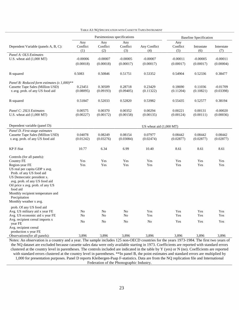
23

TABLE A3: NQ SPECIFICATION WITH CASSETTE TAPES INSTRUMENT

Parsimonious specifications Baseline Specification

Dependent Variable (panels A, B, C): Any

Conflict (1)

Any Conflict

(2)

Any Conflict

(3) Any Conflict

(4)

Any Conflict

(5) Intrastate

(6) Interstate

(7) Panel A: OLS Estimates U.S. wheat aid (1,000 MT) -0.00006 -0.00007 -0.00005 -0.00007 -0.00011 -0.00005 -0.00011

(0.00018) (0.00018) (0.00017) (0.00017) (0.00017) (0.00017) (0.00004)

R-squared 0.5083 0.50846 0.51751 0.53352 0.54904 0.52336 0.38477

Panel B: Reduced form estimates (x 1,000)**

Cassette Tape Sales (Million USD) 0.23451 0.30509 0.28718 0.23429 0.18690 0.11036 -0.01709 x avg. prob. of any US food aid (0.08095) (0.09193) (0.09405) (0.11322) (0.11204) (0.10821) (0.03398)

R-squared 0.51847 0.52033 0.52820 0.53982 0.55435 0.52577 0.38194

Panel C: 2SLS Estimates 0.00575 0.00370 0.00352 0.00294 0.00221 0.00131 -0.00020 U.S. wheat aid (1,000 MT) (0.00227) (0.00172) (0.00158) (0.00135) (0.00124) (0.00111) (0.00036)

Dependent variable (panel D): US wheat aid (1,000 MT) Panel D. First-stage estimates Cassette Tape Sales (Million USD) 0.04078 0.08249 0.08154 0.07977 0.08442 0.08442 0.08442 x avg. prob. of any US food aid (0.01242) (0.03276) (0.03084) (0.02474) (0.02877) (0.02877) (0.02877)

KP F-Stat 10.77 6.34 6.99 10.40 8.61 8.61 8.61

Controls (for all panels): Country FE Yes Yes Yes Yes Yes Yes Yes Region-year FE Yes Yes Yes Yes Yes Yes Yes US real per capita GDP x avg. Prob. of any US food aid US Democratic president x. avg. prob. of any US food aid Oil price x avg. prob. of any US food aid Monthly recipient temperature and Precipitation Monthly weather x avg.

prob. Of any US food aid Avg. US military aid x year FE No No No Yes Yes Yes Yes Avg. US economic aid x year FE No No No Yes Yes Yes Yes Avg. recipient cereal imports x year FE No No No No Yes Yes Yes

Avg. recipient cereal production x year FE Observations(for all panels): 3,896 3,896 3,896 3,896 3,896 3,896 3,896 Notes: An observation is a country and a year. The sample includes 125 non-OECD countries for the years 1973-1984. The first two years of the NQ dataset are excluded because cassette sales data were only available starting in 1973. Coefficients are reported with standard errors clustered at the country level in parentheses. The controls included are indicated in the table by Y (yes) or N (no). Coefficients are reported

with standard errors clustered at the country level in parentheses. **In panel B, the point estimates and standard errors are multiplied by 1,000 for presentation purposes. Panel D reports Kleibergen-Paap F-statistics. Data are from the NQ replication file and International

Federation of the Phonographic Industry.

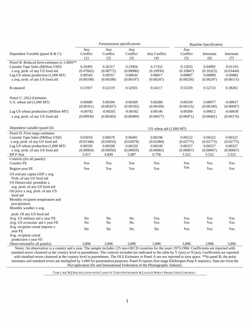
1

TABLE A4: NQ SPECIFICATION WITH CASSETTE TAPES INSTRUMENT & LAGGED WHEAT PRODUCTION CONTROLS

Parsimonious specifications Baseline Specification

Dependent Variable (panel B & C): Any

Conflict (1)

Any Conflict

(2)

Any Conflict

(3) Any Conflict

(4)

Any Conflict

(5) Intrastate

(6) Interstate

(7) Panel B: Reduced form estimates (x 1,000)**

Cassette Tape Sales (Million USD) 0.20495 0.26317 0.23956 0.17352 0.12655 0.04992 -0.01103 x avg. prob. of any US food aid (0.07843) (0.08772) (0.08986) (0.10930) (0.10847) (0.10323) (0.03444) Lag US wheat production (1,000 MT) 0.00543 0.00557 0.00630 0.00817 0.00807 0.00809 -0.00081 x avg. prob. of any US food aid (0.00198) (0.00188) (0.00197) (0.00247) (0.00256) (0.00247) (0.00115)

R-squared 0.51937 0.52119 0.52925 0.54117 0.55559 0.52723 0.38202

Panel C: 2SLS Estimates U.S. wheat aid (1,000 MT) 0.00680 0.00394 0.00369 0.00280 0.00194 0.00077 -0.00017 (0.00351) (0.00207) (0.00192) (0.00169) (0.00155) (0.00140) (0.00047) Lag US wheat production (Million MT) -0.00782 -0.00265 -0.00182 0.00146 0.00309 0.00612 -0.00038 x avg. prob. of any US food aid (0.00936) (0.00383) (0.00409) (0.00477) (0.00471) (0.00401) (0.00176)

Dependent variable (panel D): US wheat aid (1,000 MT) Panel D. First-stage estimates Cassette Tape Sales (Million USD) 0.03016 0.06679 0.06491 0.06196 0.06522 0.06522 0.06522 x avg. prob. of any US food aid (0.01346) (0.03033) (0.02878) (0.02384) (0.02775) (0.02775) (0.02775) Lag US wheat production (1,000 MT) 0.00195 0.00208 0.00220 0.00240 0.00257 0.00257 0.00257 x avg. prob. of any US food aid (0.00064) (0.00056) (0.00059) (0.00065) (0.00067) (0.00067) (0.00067) KP F-Stat 5.017 4.849 5.087 6.758 5.522 5.522 5.522 Controls (for all panels): Country FE Yes Yes Yes Yes Yes Yes Yes Region-year FE Yes Yes Yes Yes Yes Yes Yes US real per capita GDP x avg. Prob. of any US food aid US Democratic president x. avg. prob. of any US food aid Oil price x avg. prob. of any US food aid Monthly recipient temperature and precipitation Monthly weather x avg.

prob. Of any US food aid Avg. US military aid x year FE No No No Yes Yes Yes Yes Avg. US economic aid x year FE No No No Yes Yes Yes Yes Avg. recipient cereal imports x year FE No No No No Yes Yes Yes

Avg. recipient cereal production x year FE Observations(for all panels): 3,896 3,896 3,896 3,896 3,896 3,896 3,896

Notes: An observation is a country and a year. The sample includes 125 non-OECD countries for the years 1973-1984. Coefficients are reported with standard errors clustered at the country level in parentheses. The controls included are indicated in the table by Y (yes) or N (no). Coefficients are reported

with standard errors clustered at the country level in parentheses. The OLS Estimates in Panel A are not reported to save space. **In panel B, the point estimates and standard errors are multiplied by 1,000 for presentation purposes. Panel D reports first-stage Kleibergen-Paap F-statistics. Data are from the

NQ replication file and International Federation of the Phonographic Industry.

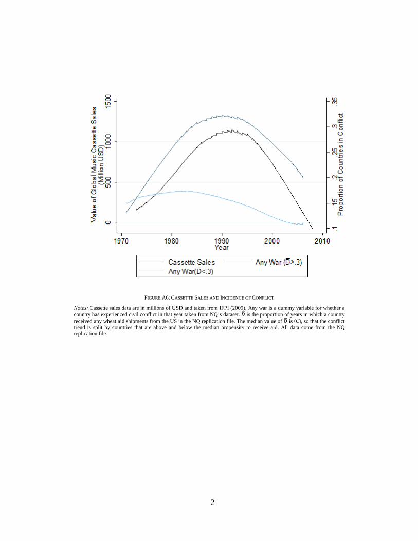
2

FIGURE A6: CASSETTE SALES AND INCIDENCE OF CONFLICT

Notes: Cassette sales data are in millions of USD and taken from IFPI (2009). Any war is a dummy variable for whether a country has experienced civil conflict in that year taken from NQ’s dataset. 𝐷𝐷� is the proportion of years in which a country received any wheat aid shipments from the US in the NQ replication file. The median value of 𝐷𝐷� is 0.3, so that the conflict trend is split by countries that are above and below the median propensity to receive aid. All data come from the NQ replication file.

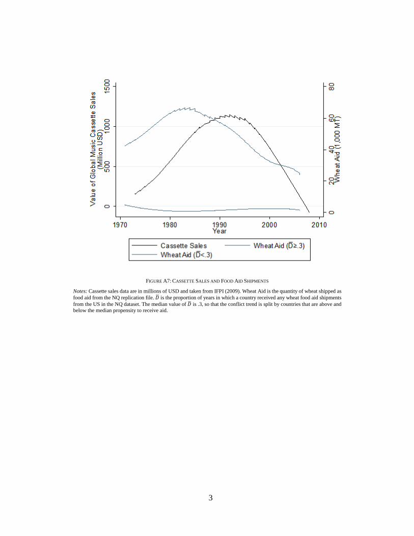
3

FIGURE A7: CASSETTE SALES AND FOOD AID SHIPMENTS

Notes: Cassette sales data are in millions of USD and taken from IFPI (2009). Wheat Aid is the quantity of wheat shipped as food aid from the NQ replication file. 𝐷𝐷� is the proportion of years in which a country received any wheat food aid shipments from the US in the NQ dataset. The median value of 𝐷𝐷� is .3, so that the conflict trend is split by countries that are above and below the median propensity to receive aid.

4

Appendix 4. A Monte Carlo Assessment of the Effect of Long Run Time

Trends in the Nunn and Qian Estimation Strategy

A. A simple model of the confounding effect of trends

NQ rely on predicting changes in aid through changes in the total quantity of

wheat produced in the US. Since they argue that wheat production is mostly a

function of climatic changes, then variation in aid conditional on climate is

plausibly exogenous. This is an appealing argument if wheat production varies

considerably from year to year so that wheat production in adjacent years is

unrelated, because it would be hard to explain fluctuations in aid and conflict that

vary from year to year in exactly the same way as wheat. As we show below,

however, wheat production and conflict in regular aid recipients both show

pronounced parallel trend patterns in the time series. Given that the trend in conflict

incidence in irregular aid recipients does not parallel the others, these trends can

generate spurious correlation that fully explains the NQ results, much like the

violation of the parallel trends assumption in DID estimation can lead to spurious

results.

We motivate the importance of these patterns by presenting a simple model that

highlights how persistent and parallel trends of wheat production and conflict can

generate patterns similar to those reported by NQ without any underlying causal

effect of aid producing or extending conflict. We then simulate coefficient

estimates using the NQ estimation strategy to show via Monte Carlo analysis that

even when food aid flows do not cause conflict in the true data generating process

(DGP), the NQ estimation strategy yield estimates spuriously suggesting a causal

effect in the presence of these heterogeneous trends among potentially endogenous

groups.

Suppose that wheat production follows the following pattern:

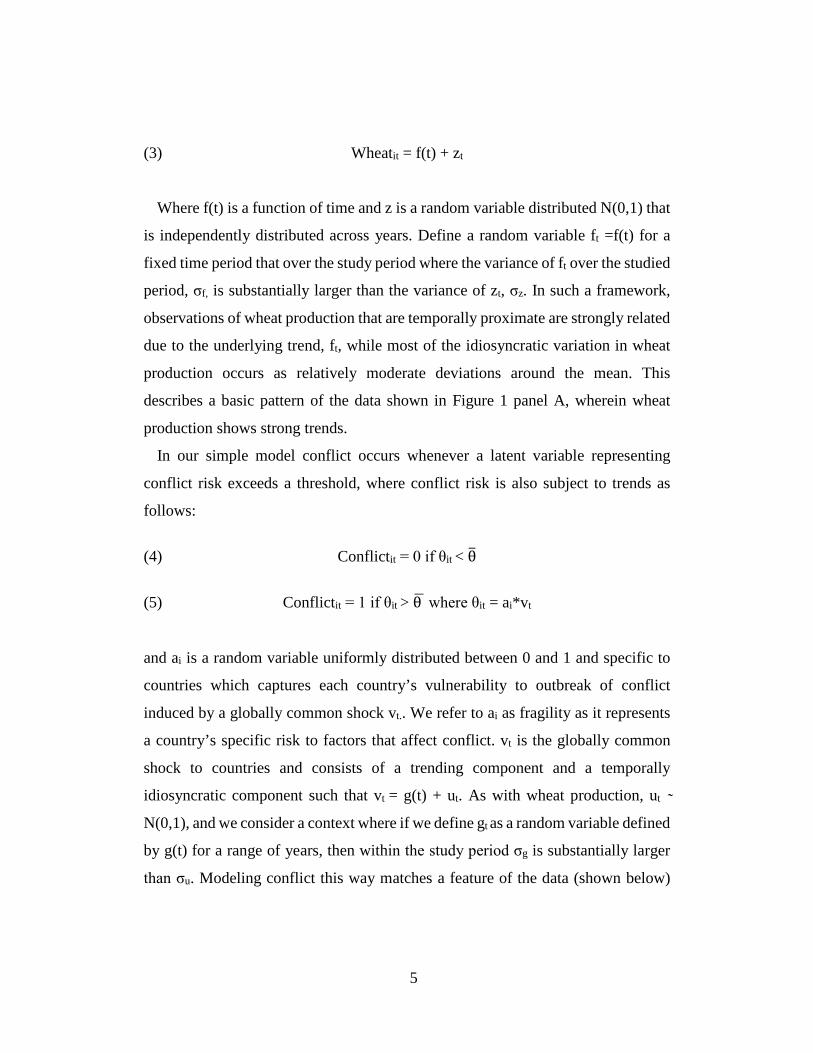
5

(3) Wheatit = f(t) + zt

Where f(t) is a function of time and z is a random variable distributed N(0,1) that

is independently distributed across years. Define a random variable ft =f(t) for a

fixed time period that over the study period where the variance of ft over the studied

period, σf, is substantially larger than the variance of zt, σz. In such a framework,

observations of wheat production that are temporally proximate are strongly related

due to the underlying trend, ft, while most of the idiosyncratic variation in wheat

production occurs as relatively moderate deviations around the mean. This

describes a basic pattern of the data shown in Figure 1 panel A, wherein wheat

production shows strong trends.

In our simple model conflict occurs whenever a latent variable representing

conflict risk exceeds a threshold, where conflict risk is also subject to trends as

follows:

(4) Conflictit = 0 if θit < θ�

(5) Conflictit = 1 if θit > θ � where θit = ai*vt

and ai is a random variable uniformly distributed between 0 and 1 and specific to

countries which captures each country’s vulnerability to outbreak of conflict

induced by a globally common shock vt.. We refer to ai as fragility as it represents

a country’s specific risk to factors that affect conflict. vt is the globally common

shock to countries and consists of a trending component and a temporally

idiosyncratic component such that vt = g(t) + ut. As with wheat production, ut ̴

N(0,1), and we consider a context where if we define gt as a random variable defined

by g(t) for a range of years, then within the study period σg is substantially larger

than σu. Modeling conflict this way matches a feature of the data (shown below)

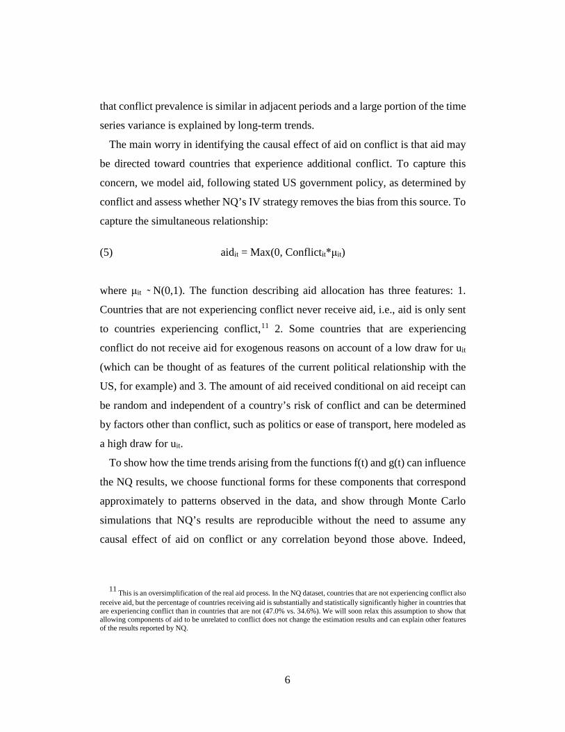
6

that conflict prevalence is similar in adjacent periods and a large portion of the time

series variance is explained by long-term trends.

The main worry in identifying the causal effect of aid on conflict is that aid may

be directed toward countries that experience additional conflict. To capture this

concern, we model aid, following stated US government policy, as determined by

conflict and assess whether NQ’s IV strategy removes the bias from this source. To

capture the simultaneous relationship:

(5) aidit = Max(0, Conflictit*μit)

where μit ̴ N(0,1). The function describing aid allocation has three features: 1.

Countries that are not experiencing conflict never receive aid, i.e., aid is only sent

to countries experiencing conflict,11 2. Some countries that are experiencing

conflict do not receive aid for exogenous reasons on account of a low draw for uit

(which can be thought of as features of the current political relationship with the

US, for example) and 3. The amount of aid received conditional on aid receipt can

be random and independent of a country’s risk of conflict and can be determined

by factors other than conflict, such as politics or ease of transport, here modeled as

a high draw for uit.

To show how the time trends arising from the functions f(t) and g(t) can influence

the NQ results, we choose functional forms for these components that correspond

approximately to patterns observed in the data, and show through Monte Carlo

simulations that NQ’s results are reproducible without the need to assume any

causal effect of aid on conflict or any correlation beyond those above. Indeed,

11 This is an oversimplification of the real aid process. In the NQ dataset, countries that are not experiencing conflict also

receive aid, but the percentage of countries receiving aid is substantially and statistically significantly higher in countries that are experiencing conflict than in countries that are not (47.0% vs. 34.6%). We will soon relax this assumption to show that allowing components of aid to be unrelated to conflict does not change the estimation results and can explain other features of the results reported by NQ.

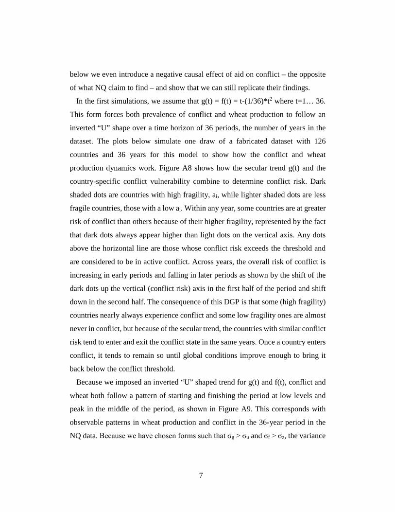
7

below we even introduce a negative causal effect of aid on conflict – the opposite

of what NQ claim to find – and show that we can still replicate their findings.

In the first simulations, we assume that g(t) = f(t) = t-(1/36)*t2 where t=1… 36.

This form forces both prevalence of conflict and wheat production to follow an

inverted “U” shape over a time horizon of 36 periods, the number of years in the

dataset. The plots below simulate one draw of a fabricated dataset with 126

countries and 36 years for this model to show how the conflict and wheat

production dynamics work. Figure A8 shows how the secular trend g(t) and the

country-specific conflict vulnerability combine to determine conflict risk. Dark

shaded dots are countries with high fragility, ai, while lighter shaded dots are less

fragile countries, those with a low ai. Within any year, some countries are at greater

risk of conflict than others because of their higher fragility, represented by the fact

that dark dots always appear higher than light dots on the vertical axis. Any dots

above the horizontal line are those whose conflict risk exceeds the threshold and

are considered to be in active conflict. Across years, the overall risk of conflict is

increasing in early periods and falling in later periods as shown by the shift of the

dark dots up the vertical (conflict risk) axis in the first half of the period and shift

down in the second half. The consequence of this DGP is that some (high fragility)

countries nearly always experience conflict and some low fragility ones are almost

never in conflict, but because of the secular trend, the countries with similar conflict

risk tend to enter and exit the conflict state in the same years. Once a country enters

conflict, it tends to remain so until global conditions improve enough to bring it

back below the conflict threshold.

Because we imposed an inverted “U” shaped trend for g(t) and f(t), conflict and

wheat both follow a pattern of starting and finishing the period at low levels and

peak in the middle of the period, as shown in Figure A9. This corresponds with

observable patterns in wheat production and conflict in the 36-year period in the

NQ data. Because we have chosen forms such that σg > σu and σf > σz, the variance

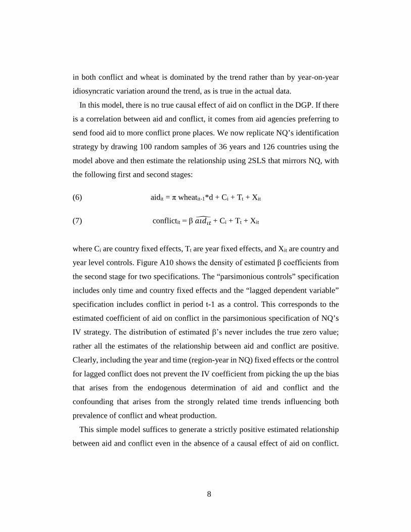
8

in both conflict and wheat is dominated by the trend rather than by year-on-year

idiosyncratic variation around the trend, as is true in the actual data.

In this model, there is no true causal effect of aid on conflict in the DGP. If there

is a correlation between aid and conflict, it comes from aid agencies preferring to

send food aid to more conflict prone places. We now replicate NQ’s identification

strategy by drawing 100 random samples of 36 years and 126 countries using the

model above and then estimate the relationship using 2SLS that mirrors NQ, with

the following first and second stages:

(6) aidit = π wheatit-1*d + Ci + Tt + Xit

(7) conflictit = β 𝑎𝑎𝑎𝑎𝑑𝑑𝚤𝚤𝚤𝚤� + Ci + Tt + Xit

where Ci are country fixed effects, Tt are year fixed effects, and Xit are country and

year level controls. Figure A10 shows the density of estimated β coefficients from

the second stage for two specifications. The “parsimonious controls” specification

includes only time and country fixed effects and the “lagged dependent variable”

specification includes conflict in period t-1 as a control. This corresponds to the

estimated coefficient of aid on conflict in the parsimonious specification of NQ’s

IV strategy. The distribution of estimated β’s never includes the true zero value;

rather all the estimates of the relationship between aid and conflict are positive.

Clearly, including the year and time (region-year in NQ) fixed effects or the control

for lagged conflict does not prevent the IV coefficient from picking the up the bias

that arises from the endogenous determination of aid and conflict and the

confounding that arises from the strongly related time trends influencing both

prevalence of conflict and wheat production.

This simple model suffices to generate a strictly positive estimated relationship

between aid and conflict even in the absence of a causal effect of aid on conflict.

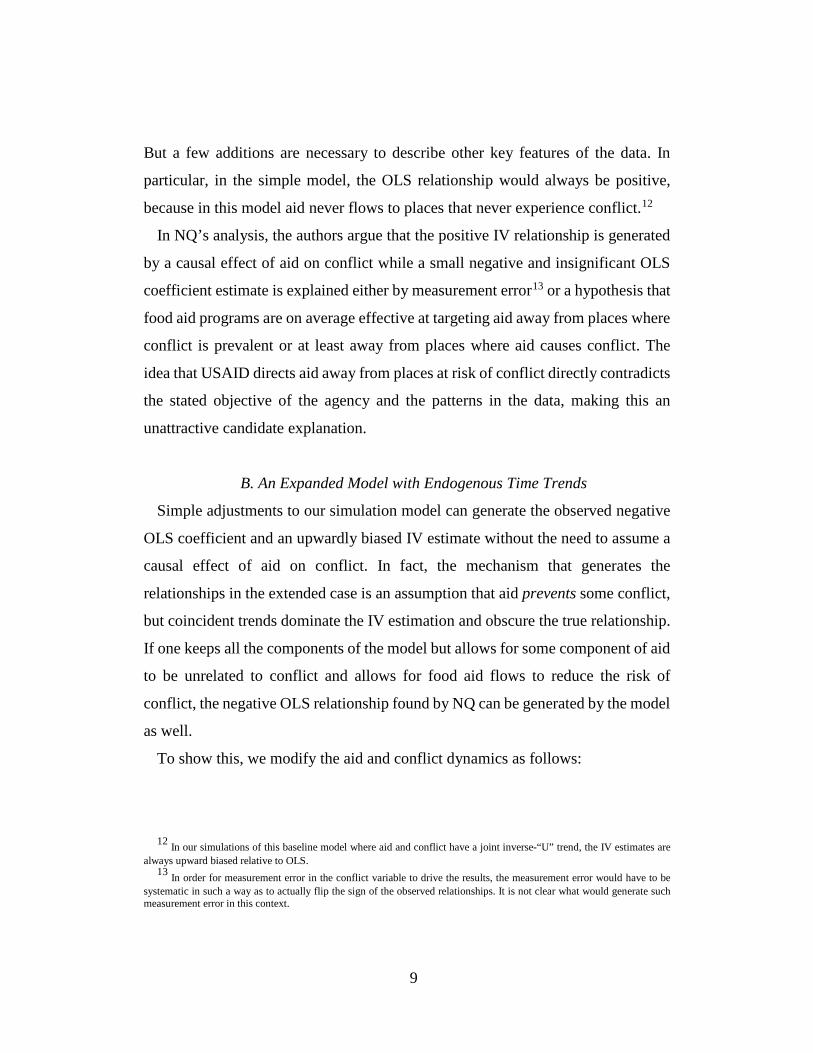
9

But a few additions are necessary to describe other key features of the data. In

particular, in the simple model, the OLS relationship would always be positive,

because in this model aid never flows to places that never experience conflict.12

In NQ’s analysis, the authors argue that the positive IV relationship is generated

by a causal effect of aid on conflict while a small negative and insignificant OLS

coefficient estimate is explained either by measurement error13 or a hypothesis that

food aid programs are on average effective at targeting aid away from places where

conflict is prevalent or at least away from places where aid causes conflict. The

idea that USAID directs aid away from places at risk of conflict directly contradicts

the stated objective of the agency and the patterns in the data, making this an

unattractive candidate explanation.

B. An Expanded Model with Endogenous Time Trends

Simple adjustments to our simulation model can generate the observed negative

OLS coefficient and an upwardly biased IV estimate without the need to assume a

causal effect of aid on conflict. In fact, the mechanism that generates the

relationships in the extended case is an assumption that aid prevents some conflict,

but coincident trends dominate the IV estimation and obscure the true relationship.

If one keeps all the components of the model but allows for some component of aid

to be unrelated to conflict and allows for food aid flows to reduce the risk of

conflict, the negative OLS relationship found by NQ can be generated by the model

as well.

To show this, we modify the aid and conflict dynamics as follows:

12 In our simulations of this baseline model where aid and conflict have a joint inverse-“U” trend, the IV estimates are

always upward biased relative to OLS. 13 In order for measurement error in the conflict variable to drive the results, the measurement error would have to be

systematic in such a way as to actually flip the sign of the observed relationships. It is not clear what would generate such measurement error in this context.

10

(8) Aidit = Max(0, I(θit > θ � )*uit) + wit

Where wit = 2*Max(0, ηit) with probability .5

0 with probability .5

ηit ̴ N(0,1)

The new aid function allows the possibility that not all food aid is determined by

conflict. Rather, food aid flows can vary on both the intensive and extensive margin

in idiosyncratic ways, for example because aid may be shipped as a response to

natural disasters. The component of aid that arises for these reasons is described by

wit, which has two sources of idiosyncratic variation. The first part, ηit, represents

the part that is correlated with the quantity of the food aid shipment, for example,

the intensity of a natural disaster. The second part is the exogenous reasons that a

country with a positive draw of ηit will receive any aid or not. This is modeled by

the fact that a given country in a given year that has a positive draw of ηit has a 50%

chance of receiving aid and a 50% chance of not receiving aid.

In contrast to the earlier model, there are now two reasons that countries receive

food aid. The proportion of countries experiencing conflict will vary by year, but

in expectation, 50% of the countries experiencing conflict will receive some aid

because of their conflict status. Aid for non-conflict reasons such as disasters does

not systematically vary by time. In expectation, 50% of countries will experience a

disaster that warrants aid shipments, and 50% of the countries that experience such

a shock receive aid.

The second modification is that aid flows can prevent conflict, as advocates of

food aid hope. We now modify the model so that if a country receives aid for any

reason, either because of a high risk of conflict or because of a disaster, it will not

experience conflict in that year. Thus, all countries that would experience conflict

(those with θit > θ �) can receive aid, but only some receive it. Any countries that

11

receive aid for this reason or because of the idiosyncratic component wt will not

experience conflict in that year so that:

(8) Conflictit = 0 if Aidit>0

These modifications to the model capture several plausible features of the true

DGP:

1. Countries that are at risk of conflict are likely to get aid for that reason.

2. Countries also receive aid for idiosyncratic reasons that are not related

to conflict, such as political considerations, natural disasters, etc.

3. Aid can prevent conflict, for example by alleviating the conditions that

cause people to fight or because delivery of US food aid is associated

with actions and investments that control conflict, such as the

deployment of peacekeeping troops.

Modifying the model in this way and repeating the Monte Carlo simulation 100

times leads to the distribution of OLS and IV coefficients shown in Figure A11.

The OLS relationship from NQ’s specification is negative in all instances of the

simulation, just as they find, reflecting the fact that although countries that

experience conflict receive the most aid, they experience conflict only in the years

when for exogenous reasons they do not actually receive aid. The IV relationship

is still positive due to the parallel time trends problem. The negative OLS estimates

capture the effects of aid flows that arise both because of conflict risk and other

unrelated sources. The instrument misleadingly focuses on differences in aid that

are endogenous to conflict for two reasons. Countries that experience the most

conflict are most likely to get aid and conflict and wheat production are spuriously

related over time.

These results highlight the fact that a comparison of the OLS results with the IV

results in NQ’s analysis does not compel a conclusion that aid causes conflict. In

12

fact, in the expanded model above, the same parameter estimate patterns they find

appear in a context where aid actually prevents rather than causes conflict.

C. A Low Power Robustness Test

NQ recognize that spurious time trends could be a threat to identification of

causal effects, so they propose and implement a robustness check to assess whether

trends drive their relationship between wheat production and food aid flows. In

their primary specification, they report the effect of their instrument on current food

aid volumes. As a robustness check, they compare this correlation to the estimated

relationship between their instrument and aid lagged by two periods. They argue

that lagged aid could not be causally related to current wheat production, but would

show a similar relationship as their first stage if spurious trends were behind the

observed relationship. In their view, failing to find a correlation between current

wheat production and past wheat aid provides suggestive evidence that trends do

not account for their first stage. They find a positive and statistically significant

effect of their instrument on current wheat aid, but a small negative and statistically

significant relationship between the instrument and past aid. They argue that the

lack of relationship between wheat and past aid supports their assertion that

spurious trends are not behind their results.

But conflict and aid in both reality and in our Monte Carlo model are functions

not only of the time trends but also current period shocks. It is possible that while

the IV estimates a positive relationship in contemporaneous periods, it may not

identify an effect on conflict lagged by two periods. To test how compelling this

robustness check is as a test of whether secular trends could drive their result, we

implement the test on our simulated dataset. If this robustness check is convincing,

we should find that the main IV specification and the correlation of wheat

production with past wheat food aid should show a similar distribution. If, however,

13

the coefficients on the instrument in separate regressions on contemporaneous and

lagged aid are dissimilar, the robustness check is not convincing.

Figure A12 shows the density of estimated coefficients between the instrument

and the dependent variables in NQ’s preferred first stage (current aid) and the

dependent variable of the robustness check (past aid) for our expanded model.

The coefficient on the instrument as a regressor for current aid is positive in all

draws of the simulation suggesting that wheat production is associated with

additional wheat food aid shipments to preferred recipients. The distribution of

estimated coefficients from regressing twice lagged aid on the instrument falls

largely to the left of the first stage coefficients, and is close to zero. These

simulations show that this robustness check has very low power to diagnose the

trend problem and should not be taken as evidence that trends do not underlie the

results NQ present.

D. Potential Sources of Coincident Trends in Wheat Production, Aid, and

Conflict

One of the fundamental assumptions for identifying a causal effect from an IV

strategy is that conditional on the controls, the instrument is related to the dependent

variable of interest only through its correlation with the endogenous regressor.

Given the diversity of factors that could be related to both wheat production and

conflict at a global scale – many of them, such as geopolitical factors, difficult to

measure – and the complex ways in which the effect of a particular factor on

conflict or aid may manifest, it is unlikely that we can adequately control for all

factors.

It is nevertheless worth asking whether including linear controls for these

variables, as NQ do, solves the problem. We therefore explore how heterogeneous

14

effects of variables potentially driving the observed trends can undermine the

effectiveness of the controls. Given that there are alternative channels linking wheat

production and conflict, the role of controls in validating this assumption is crucial.

We focus here on one source of potential violation of the exclusion restriction and

assess the role of model specification to demonstrate that without a very clear

understanding of exactly how conflict is determined, it is difficult to use controls

in a way that recovers the causal interpretation.

An obvious candidate variable that jointly causes conflict and wheat production

is climatic variation. Fluctuations in rainfall or temperature are important

determinants of wheat production in the US (Barkley et al, 2013) and may be related

to fluctuations globally because the global climate is a closed system. Weather and

rainfall are well known to be related to conflict risk (Hsiang, Burke, Miguel, 2013).

To address this concern, NQ include controls for monthly mean temperature and

precipitation.

But this is not sufficient to preclude any partial relationship between residual

weather and conflict, as weather fluctuations can involve far more than mean

temperature and rainfall. For example, (Hsiang, Meng, and Cane, 2011) show that

surface ocean temperature variation associated with ENSO – a multi-year climate

cycle in which surface ocean temperatures oscillate between warm and cool periods

(called El Niño and La Niña, respectively) – is related to global conflict risk, even

controlling for monthly temperature, rainfall, and cyclonic windspeed. These

oscillations cause global fluctuations in weather that have recently been strongly

linked with global wheat production (Iizumi et al, 2014), macroeconomic

performance (Cashin et al, 2014) and conflict (Hsiang, Meng, and Cane, 2011). In

this example, we therefore use variation in sea surface temperatures associated with

the ENSO phenomenon.

NQ’s claim that including average monthly precipitation and temperature in

recipient countries eliminates weather as a channel for bias rests on two important

15

assumptions. First, average monthly precipitation and temperature must fully

capture all the impacts of weather. Despite the Hsiang, Meng, and Cane (2011)

result, we find that adding their ENSO measure as an additional control does not

qualitatively alter NQ’s core result.14

The second and more problematic assumption is that the effects of weather events

like ENSO variation are constant within countries across years and across countries

within years. To demonstrate how non-constant effects of weather and climate

variation can be problematic, we simulate conflict risk as a product of a function of

ENSO variation and show that failing to account for heterogeneity in the

relationship between climate and conflict can generate a spuriously positive

estimated influence of aid on conflict without the need to assume that aid causes

conflict.

Figure A13 shows the trend in sea surface temperatures associated with El Niño

over the NQ study period.15 The trends are noisier than for conflict and wheat

production, but share the basic feature that temperatures were substantially lower

in the 1970s and were highest between 1980 and 1995.

To show how heterogeneity of influence omitted variables can create concerns in

the approach from the NQ paper, we model two different versions of a channel

linking El Niño oscillations to conflict with an endogenous link between aid and

conflict, and show that adding linear controls only obviates endogeneity if the

omitted variables bias arises in a very particular form. Suppose that these sea

surface temperature variations are the only factor influencing conflict risk and that

they are potentially correlated with wheat yields. Further refining the DGP in our

Monte Carlo model, suppose that conflict occurs whenever a country exceeds a

14 Details available on request. 15 The trend shown is the variable nino3_annual in Hsiang, Meng, and Cane (2014).

16

threshold level of latent conflict risk, and that conflict risk can take either of two

forms

(9) Riskit = NINOt + c where c is constant across countries and over time

(10) Riskit = f(i,t)*NINOt where f(i,t) is nonlinear in i and t

We call the first version (Equation 9) the linear model of conflict risk and the

second (Equation 10) the heterogeneous model. We simulate a version of this model

where f(i,t) = (αt – βt2)(δi – γi2) where α, β, δ, and γ are fixed parameters, t=1…32

are years and i=1…126 represent an index identifying countries. Figures A14 and

A15 show how simulated conflict risk varies by year according to the function f(i,t)

in Equation 10. In all countries, conflict risk peaks in the middle of the period,

consistent with the observed facts, but the intensity of the trend varies by country.

Similarly, conflict risk varies across countries in a nonlinear way.

Figures A14 and A15 show how the linear and heterogeneous models produce

different conflict risk. In both models, however, conflict risk is highest in the

middle period, because ENSO surface temperatures are highest in this period, but

the heterogeneous model (Equation 10, shown in Figure A16) differs in two

regards. First, the tendency of conflict risk to peak in the middle of the period is

more pronounced. Second, for any given year, conflict risk varies by country, so

that country 126 is always at the highest risk of conflict and country 1 is always at

the lowest, though risk of conflict in country 60 is higher in 1985 than for country

1 in 1970.

To demonstrate the importance of this kind heterogeneous response to conflict

risk, we simulate 100 draws of the system where

(11) Conflictit = 1 if θit> θ̄ where θit = riskit + εit and εit ̴ U(0, 0.01)

17

(12) Aidit = α * max(riskit - εit,0) where α is a constant

The aid allocation again captures three stylized facts about modern food aid

allocations. First, additional aid is given to countries chronically at higher risk for

conflict, as is clearly true in the data. Second, surprise realizations of conflict risk

may be associated with lower allocations in the immediate year in which they occur

because aid is more difficult to mobilize and deliver. Third, aid allocations cannot

be negative. We use the actual data for realizations of wheat production and ENSO

sea surface temperatures to simulate this system. Figure A18 shows the distribution

of coefficients of food aid and conflict using NQ’s IV strategy and their OLS

strategy for the heterogeneous model and including year and country fixed effects

(not ENSO) as controls. Clearly such a model is capable of generating the effects

shown by NQ where the OLS is modestly negative and the IV effect is positive, yet

food aid has no causal effect on conflict in the true DGP.

Figure A19 demonstrates how different relationships between ENSO and conflict

affect the key parameter estimates. In the linear model, if the ENSO variable is not

included as a control, the estimated coefficient of aid on conflict is positive, even

though we have included year and country fixed effects and have assumed that aid

is related to conflict only because more aid is sent to places that are at higher risk

for conflict. Including the ENSO control does lead to a distribution of the

coefficient that is centered around zero (the true causal effect), but only in the linear

model. Country and year fixed effects would also have solved this problem, because

across countries within a year, the influence of ENSO is constant. In the

heterogeneous model, adding the ENSO control removes some of the upward bias,

but not all of it, because the time trends in conflict differ exactly on the dimension

in which aid is endogenously allocated to countries by conflict experience in a way

that is not captured by constant linear control for ENSO.

These simulations highlight two important facts:

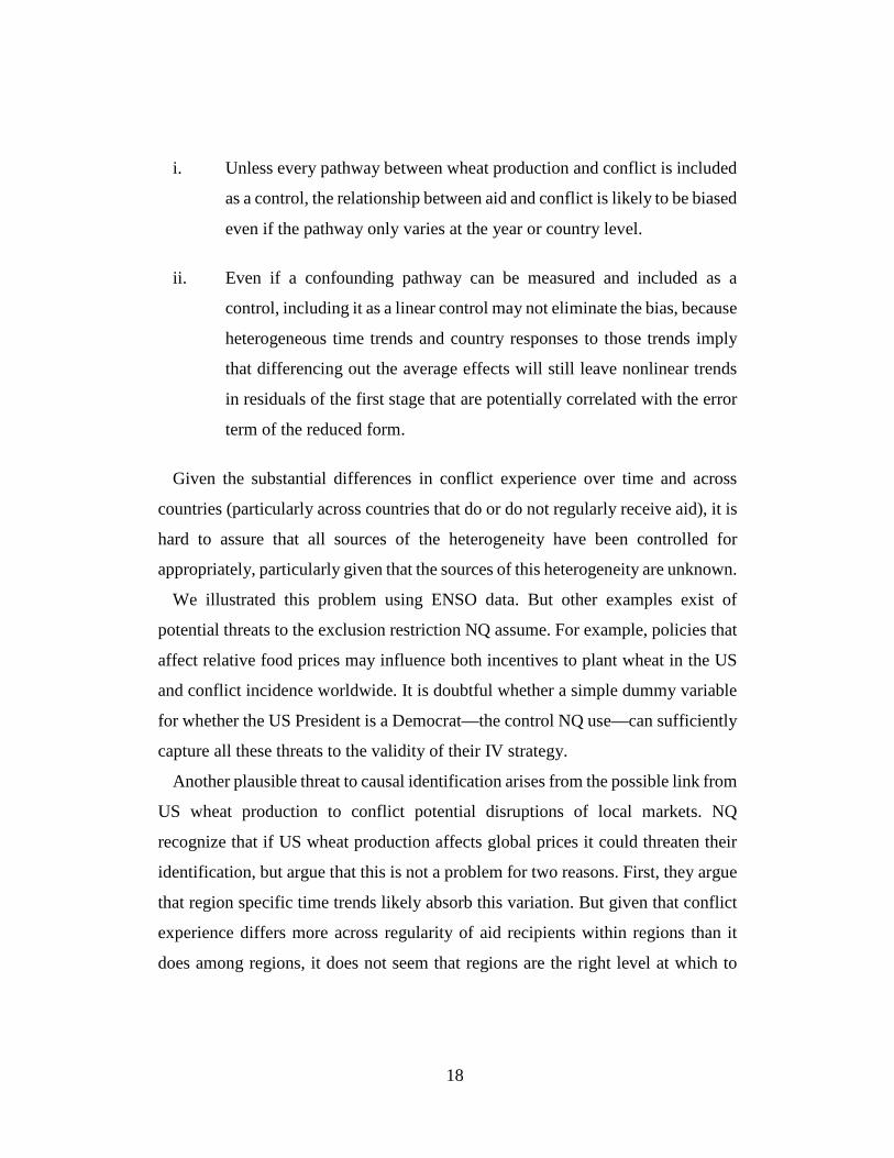
18

i. Unless every pathway between wheat production and conflict is included

as a control, the relationship between aid and conflict is likely to be biased

even if the pathway only varies at the year or country level.

ii. Even if a confounding pathway can be measured and included as a

control, including it as a linear control may not eliminate the bias, because

heterogeneous time trends and country responses to those trends imply

that differencing out the average effects will still leave nonlinear trends

in residuals of the first stage that are potentially correlated with the error

term of the reduced form.

Given the substantial differences in conflict experience over time and across

countries (particularly across countries that do or do not regularly receive aid), it is

hard to assure that all sources of the heterogeneity have been controlled for

appropriately, particularly given that the sources of this heterogeneity are unknown.

We illustrated this problem using ENSO data. But other examples exist of

potential threats to the exclusion restriction NQ assume. For example, policies that

affect relative food prices may influence both incentives to plant wheat in the US

and conflict incidence worldwide. It is doubtful whether a simple dummy variable

for whether the US President is a Democrat—the control NQ use—can sufficiently

capture all these threats to the validity of their IV strategy.

Another plausible threat to causal identification arises from the possible link from

US wheat production to conflict potential disruptions of local markets. NQ

recognize that if US wheat production affects global prices it could threaten their

identification, but argue that this is not a problem for two reasons. First, they argue

that region specific time trends likely absorb this variation. But given that conflict

experience differs more across regularity of aid recipients within regions than it

does among regions, it does not seem that regions are the right level at which to

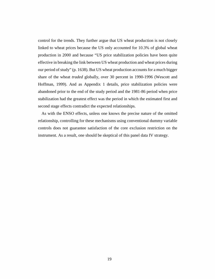
19

control for the trends. They further argue that US wheat production is not closely

linked to wheat prices because the US only accounted for 10.3% of global wheat

production in 2000 and because “US price stabilization policies have been quite

effective in breaking the link between US wheat production and wheat prices during

our period of study” (p. 1638). But US wheat production accounts for a much bigger

share of the wheat traded globally, over 30 percent in 1990-1996 (Wescott and

Hoffman, 1999). And as Appendix 1 details, price stabilization policies were

abandoned prior to the end of the study period and the 1981-86 period when price

stabilization had the greatest effect was the period in which the estimated first and

second stage effects contradict the expected relationships.

As with the ENSO effects, unless one knows the precise nature of the omitted

relationship, controlling for these mechanisms using conventional dummy variable

controls does not guarantee satisfaction of the core exclusion restriction on the

instrument. As a result, one should be skeptical of this panel data IV strategy.

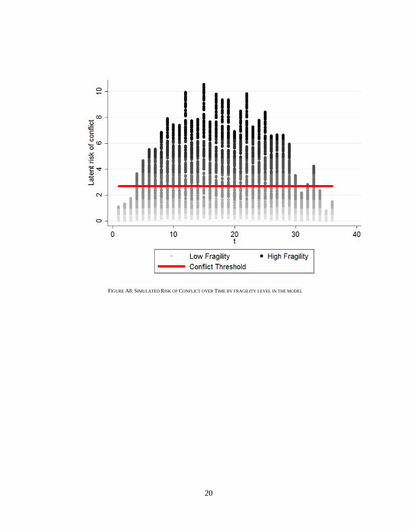
20

FIGURE A8: SIMULATED RISK OF CONFLICT OVER TIME BY FRAGILITY LEVEL IN THE MODEL

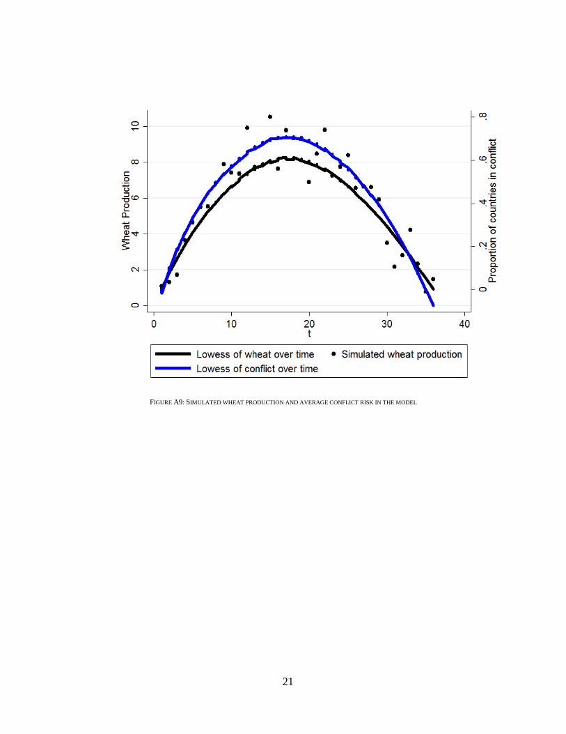
21

FIGURE A9: SIMULATED WHEAT PRODUCTION AND AVERAGE CONFLICT RISK IN THE MODEL

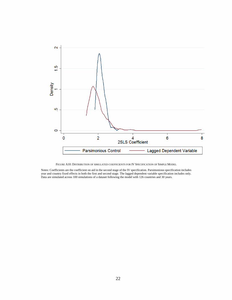
22

FIGURE A10: DISTRIBUTION OF SIMULATED COEFFICIENTS FOR IV SPECIFICATION OF SIMPLE MODEL

Notes: Coefficients are the coefficient on aid in the second stage of the IV specification. Parsimonious specification includes year and country fixed effects in both the first and second stage. The lagged dependent variable specification includes only. Data are simulated across 100 simulations of a dataset following the model with 126 countries and 30 years.

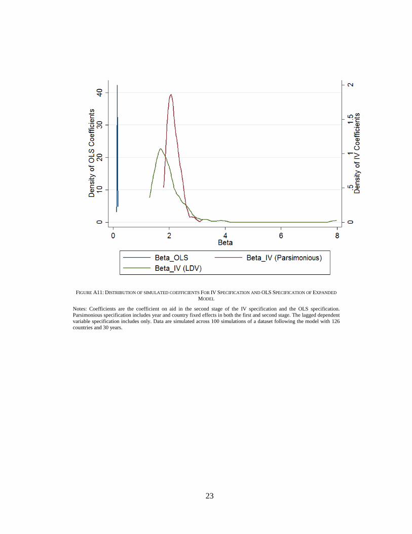
23

FIGURE A11: DISTRIBUTION OF SIMULATED COEFFICIENTS FOR IV SPECIFICATION AND OLS SPECIFICATION OF EXPANDED

MODEL

Notes: Coefficients are the coefficient on aid in the second stage of the IV specification and the OLS specification. Parsimonious specification includes year and country fixed effects in both the first and second stage. The lagged dependent variable specification includes only. Data are simulated across 100 simulations of a dataset following the model with 126 countries and 30 years.

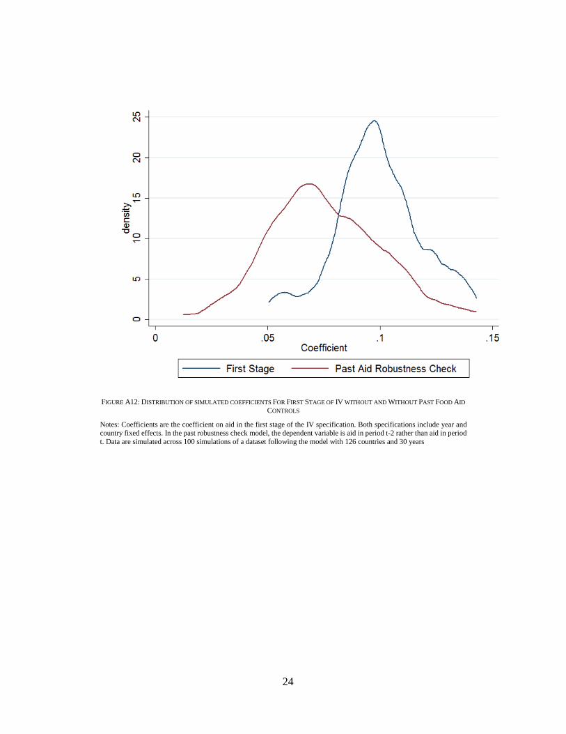
24

FIGURE A12: DISTRIBUTION OF SIMULATED COEFFICIENTS FOR FIRST STAGE OF IV WITHOUT AND WITHOUT PAST FOOD AID

CONTROLS

Notes: Coefficients are the coefficient on aid in the first stage of the IV specification. Both specifications include year and country fixed effects. In the past robustness check model, the dependent variable is aid in period t-2 rather than aid in period t. Data are simulated across 100 simulations of a dataset following the model with 126 countries and 30 years

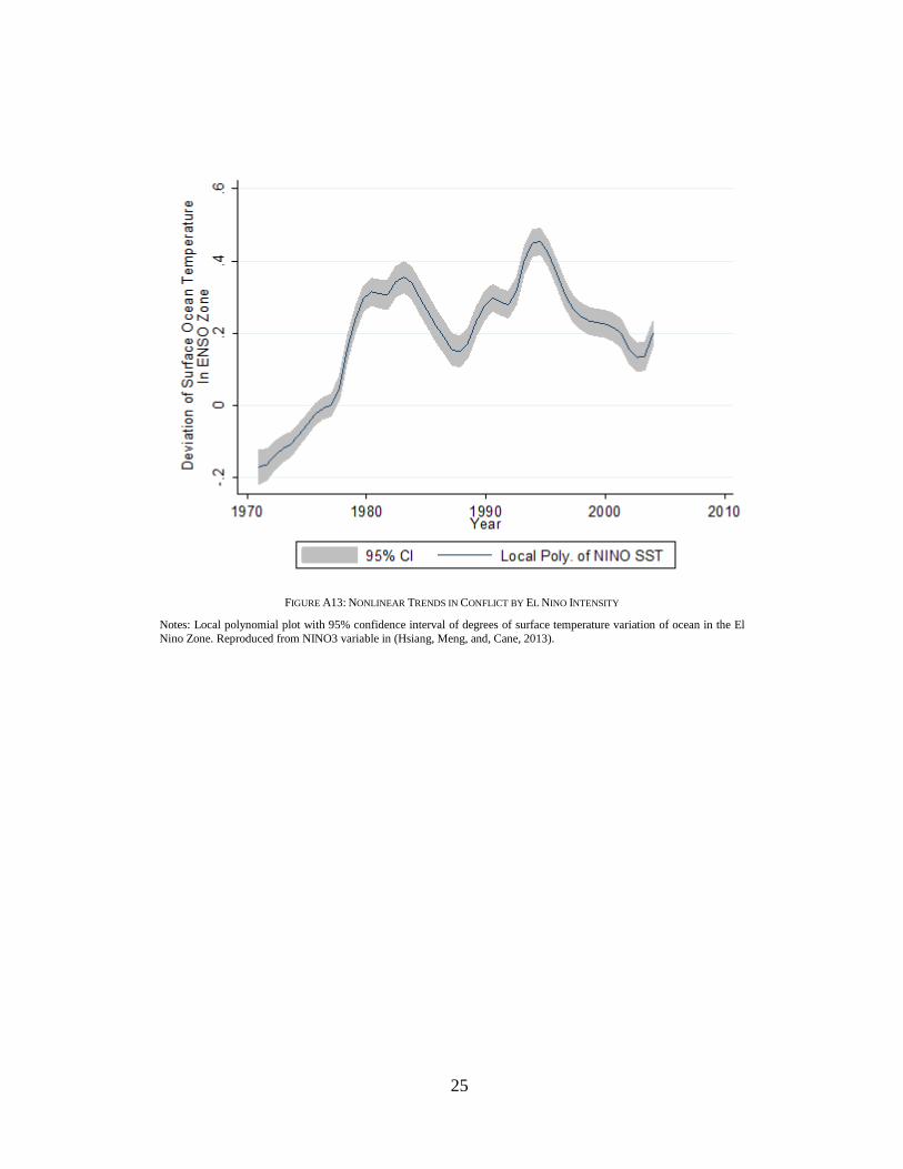
25

FIGURE A13: NONLINEAR TRENDS IN CONFLICT BY EL NINO INTENSITY

Notes: Local polynomial plot with 95% confidence interval of degrees of surface temperature variation of ocean in the El Nino Zone. Reproduced from NINO3 variable in (Hsiang, Meng, and, Cane, 2013).

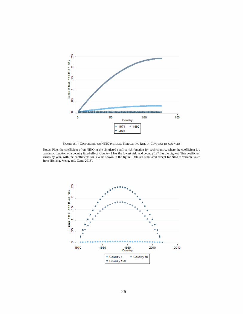
26

FIGURE A14: COEFFICIENT ON NINO IN MODEL SIMULATING RISK OF CONFLICT BY COUNTRY

Notes: Plots the coefficient of on NINO in the simulated conflict risk function for each country, where the coefficient is a quadratic function of a country fixed effect. Country 1 has the lowest risk, and country 127 has the highest. This coefficient varies by year, with the coefficients for 3 years shown in the figure. Data are simulated except for NINO3 variable taken from (Hsiang, Meng, and, Cane, 2013).

27

FIGURE A15: COEFFICIENTS ON EL NINO VARIABLE IN CONFLICT RISK FUNCTION BY YEAR AND COUNTRY

Notes: Plots the coefficient of on NINO in the simulated conflict risk function for each country, where the coefficient is a quadratic function of year. Conflict risk is lowest in the starting and ending point, and highest in the middle. The shape of the quadratic functions also depends on the country. Three countries, the highest risk, lowest risk, and moderate risk are shown. Data are simulated except for NINO3 variable taken from (Hsiang, Meng, and, Cane, 2013).

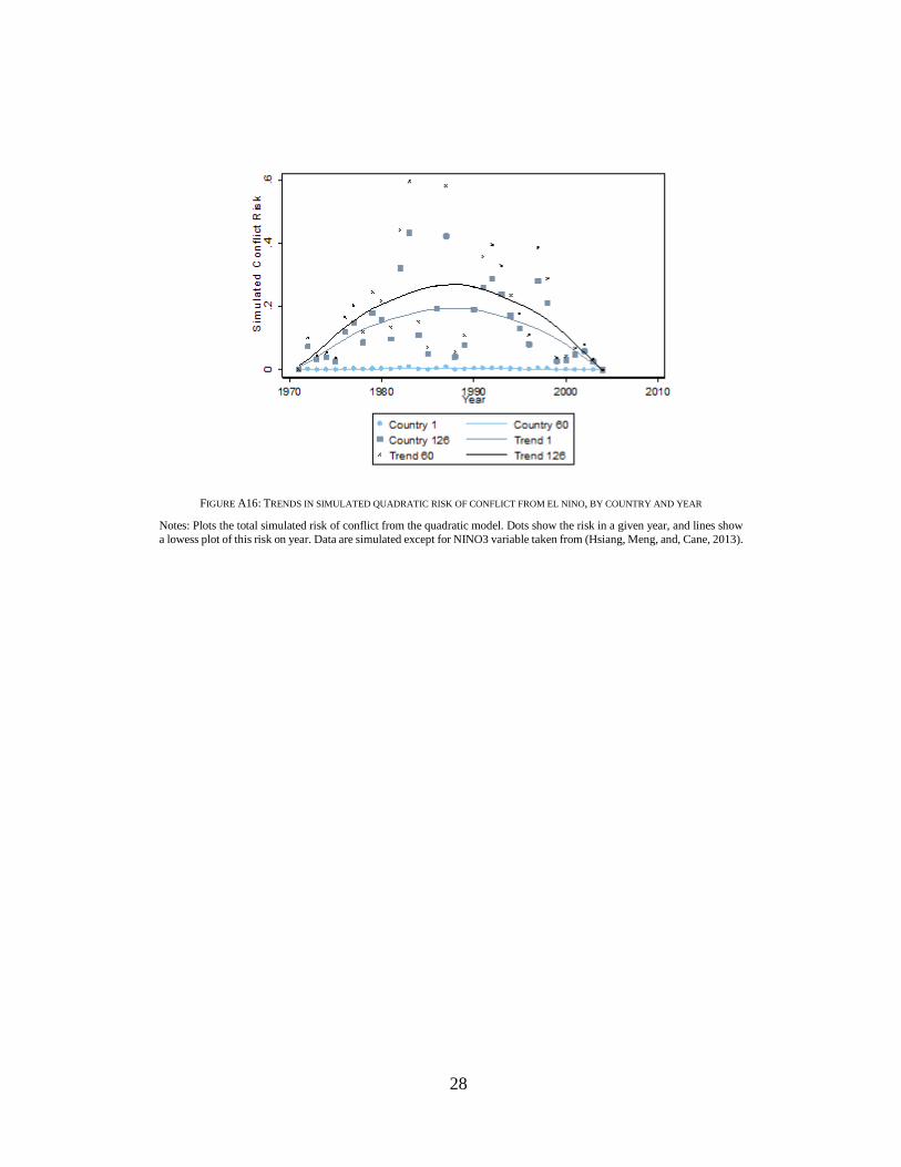
28

FIGURE A16: TRENDS IN SIMULATED QUADRATIC RISK OF CONFLICT FROM EL NINO, BY COUNTRY AND YEAR

Notes: Plots the total simulated risk of conflict from the quadratic model. Dots show the risk in a given year, and lines show a lowess plot of this risk on year. Data are simulated except for NINO3 variable taken from (Hsiang, Meng, and, Cane, 2013).

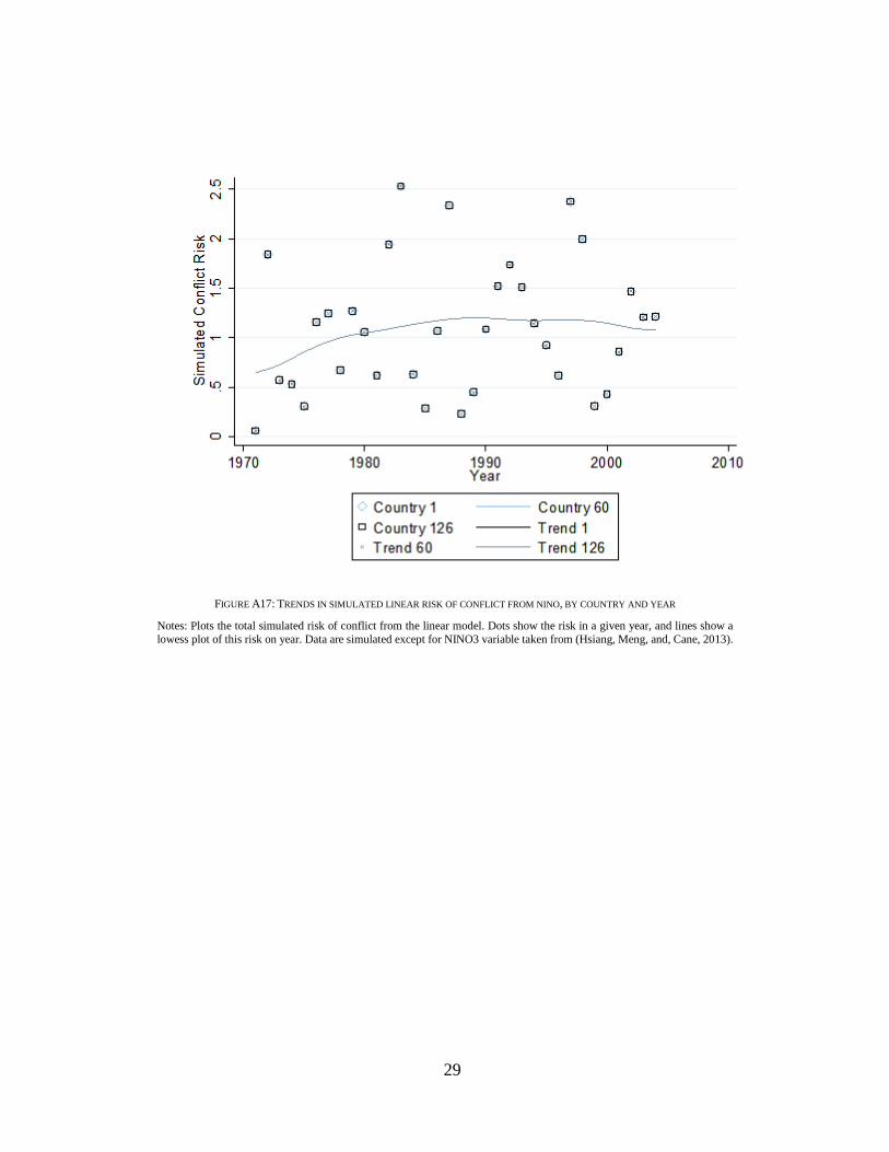
29

FIGURE A17: TRENDS IN SIMULATED LINEAR RISK OF CONFLICT FROM NINO, BY COUNTRY AND YEAR

Notes: Plots the total simulated risk of conflict from the linear model. Dots show the risk in a given year, and lines show a lowess plot of this risk on year. Data are simulated except for NINO3 variable taken from (Hsiang, Meng, and, Cane, 2013).

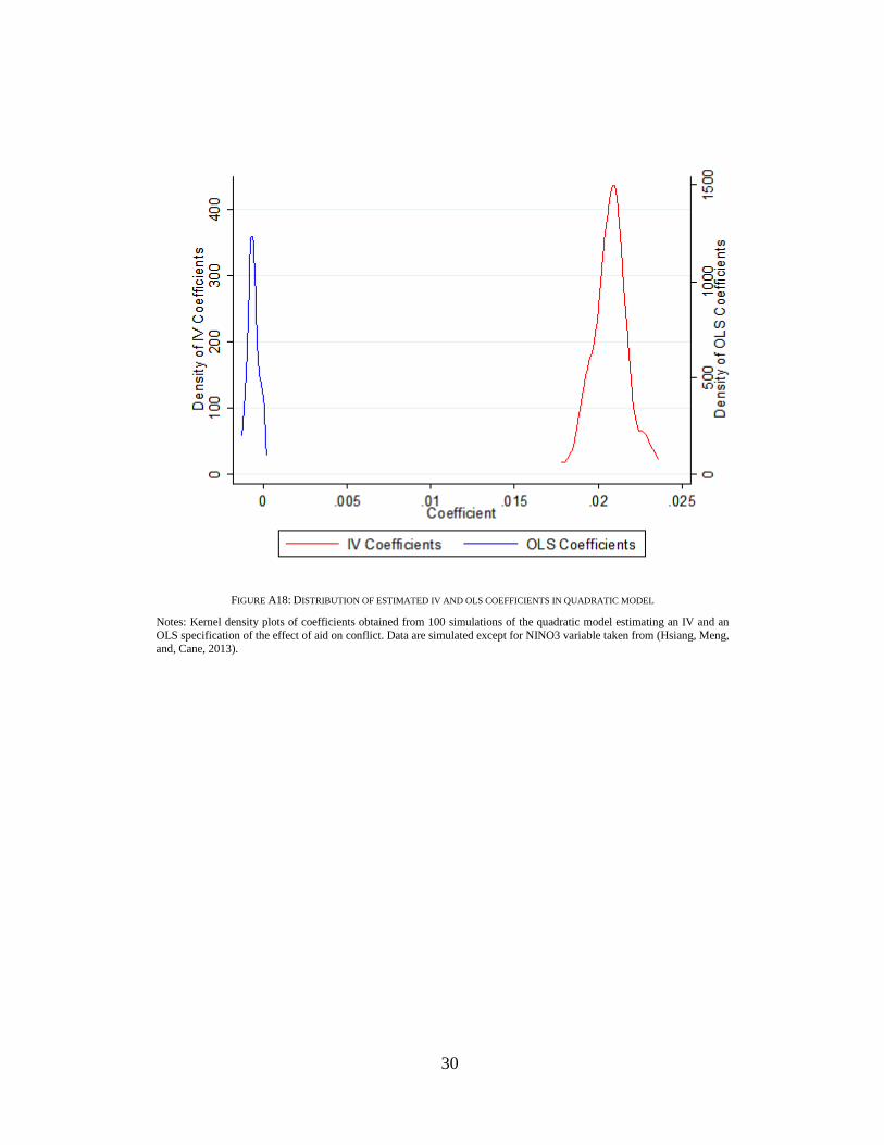
30

FIGURE A18: DISTRIBUTION OF ESTIMATED IV AND OLS COEFFICIENTS IN QUADRATIC MODEL

Notes: Kernel density plots of coefficients obtained from 100 simulations of the quadratic model estimating an IV and an OLS specification of the effect of aid on conflict. Data are simulated except for NINO3 variable taken from (Hsiang, Meng, and, Cane, 2013).

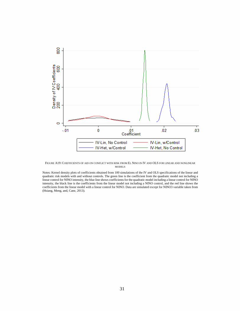
31

FIGURE A19: COEFFICIENTS OF AID ON CONFLICT WITH RISK FROM EL NINO IN IV AND OLS FOR LINEAR AND NONLINEAR

MODELS

Notes: Kernel density plots of coefficients obtained from 100 simulations of the IV and OLS specifications of the linear and quadratic risk models with and without controls. The green line is the coefficient from the quadratic model not including a linear control for NINO intensity, the blue line shows coefficients for the quadratic model including a linear control for NINO intensity, the black line is the coefficients from the linear model not including a NINO control, and the red line shows the coefficients from the linear model with a linear control for NINO. Data are simulated except for NINO3 variable taken from (Hsiang, Meng, and, Cane, 2013).

32

APPENDIX REFERENCES

Barrett, Christopher B. (1998) “Food Aid: Is It Development Assistance, Trade

Promotion, Both, or Neither?” American Journal of Agricultural Economics,

80(3): 566-571.

Barrett, Christopher B. and Kevin C. Heisey (2002). “How Effectively Does

Multilateral Food Aid Respond to Fluctuating Needs?” Food Policy. 27(5-6):

477-491.

Barrett, Christopher B. and Daniel G. Maxwell (2005). Food Aid After Fifty Years:

Recasting Its Role. New York: Routledge.

Barkley, Andrew, Jesse Tack, Lawton Lanier Nalley, Jasong Bergtold, Robert

Bowdens, Allan Fritz (2013). “The Impact of Climate, Disease, and Wheat

Breeding on Wheat Variety Yields in Kansas, 1985–2011.” Kansas State

University Agricultural Experiment Station and Cooperative Extension Service.

Bulletin 665.

Blattman, Christopher and Edward Miguel (2010). “Civil War.” Journal of

Economic Literature. 41(1): 3-57.

Cashin, Paul, Kamiar Mohaddes, Maziar Raissi, and Mehdi Raissi (2014). “The

Differential Effects of Oil Demand and Supply Shocks on the Global Economy.”

Energy Economics, 44: 113-134.

Hsiang, Solomon M., Marshall Burke, Edward Miguel (2013). “Quantifying the

Influence of Climate on Human Conflict” Science, 341, 1235367 (2013).DOI:

10.1126/science.1235367

Hsiang, Solomon M. , Kyle C. Meng & Mark A. Cane (2011). “Civil conflicts are

associated with the global climate” Nature: Letter. 476(25): 438-440.

33

Iizumi Toshichika, Jing-Jia Luo, Andrew J. Challinor, Gen Sakurai, Masayuki

Yokozawa, Hirofumi Sakuma, Molly E. Brown, and Toshio Yamagata (2014).

“Impacts of El Niño Southern Oscillation on the Global Yields of Major Crops.”

Nature Communications.5(3712).

International Federation of the Phonographic Industry. “Recording Industry in

Numbers.” Accessed 26 Aug 2015.

https://musicbusinessresearch.wordpress.com/2010/03/29/the-recession-in-the-

music-industry-a-cause-analysis/.

Jayne, Thomas S., John Strauss, Takashi Yamano, Daniel Molla (2002). “Targeting

of Food Aid in Rural Ethiopia: Chronic Need or Inertia.” Journal of Development

Economics, 68: 247-288.

Nunn, Nathan, and Nancy Qian (2014). “US Food Aid and Civil Conflict.”

American Economic Review. 104(6): 1630-66.

Schnepf, Randy (2014). “International Food Aid Programs: Background and

Issues.” Congressional Research Service.

USAID. “(Re)Assessing The Relationship Between Food Aid and Armed

Conflict.” USAID Technical Brief. October 2014.

USAID. “Office of Food for Peace.” 5 March 2015. Accessed 15 May 2015.

http://www.usaid.gov/who-we-are/organization/bureaus/bureau-democracy-

conflict-and-humanitarian-assistance/office-food

United States Department of Agriculture Economic Research Service. “Glossary.”

11 March 2014. Accessed 26 January, 2015.

http://www.ers.usda.gov/topics/farm-economy/farm-commodity-

policy/glossary.aspx

United States Department of Agriculture Farm Service Agency. “Fact Sheet:

Commodity Credit Corporation.” November 1999. Accessed 26 January, 2015.

http://www.fsa.usda.gov/Internet/FSA_File/ccc_fact_sheet.pdf

Wescott, Paul C. and Linwood A. Hoffman (1999). “Price Determination for Corn

34

and Wheat: The Role of Market Factors and Government Programs.” Market and

Trade Economics Division, Economic Research Service, U.S. Department of

Agriculture. Technical Bulletin No. 1878.

Willis, Brandon and Doug O’Brien. “Summary and Evolution of U.S. Farm Bill

Commodity Titles.” National Agriculture Law Center. Accessed 26 January

2015. http://nationalaglawcenter.org/farmbills/commodity/