Munich Personal RePEc Archive

Revisiting the Performance of MACD

and RSI Oscillators

Chong, Terence Tai-Leung and Ng, Wing-Kam and Liew,

Venus Khim-Sen

2 February 2014

Online at https://mpra.ub.uni-muenchen.de/54149/

MPRA Paper No. 54149, posted 07 Mar 2014 07:58 UTC

1

Revisiting the Performance of MACD and RSI Oscillators

Terence Tai-Leung Chong1

Hong Kong Institute of Asia-Pacific Studies, The Chinese University of Hong Kong

and

Department of International Economics and Trade, Nanjing University,

Wing-Kam Ng, Department of Economics, The Chinese University of Hong Kong

and

Venus Khim-Sen Liew

Faculty of Economics and Business, Universiti Malaysia Sarawak, Malaysia

2/2/14

Abstract: Chong and Ng (2008) find that the Moving Average Convergence-Divergence

(MACD) and Relative Strength Index (RSI) rules can generate excess return in the London

stock exchange. This paper revisits the performance of the two trading rules in the stock

markets of five other OECD countries. It is found that the MACD(12,26,0) and RSI(21,50)

rules consistently generate significant abnormal returns in the Milan Comit General and the

S&P/TSX Composite Index. In addition, the RSI(14,30/70) rule is also profitable in the Dow

Jones Industrials index. The results shed some light on investors’ believe in these two

technical indicators in different developed markets.

JEL Classification: F31; G15.

Keywords: Relative Strength Index; Trading Rules; Moving Average Convergence-

Divergence.

1 Corresponding author: Terence Chong, Department of Economics, The Chinese University of Hong Kong, Shatin, Hong Kong. Email: chong2064@cuhk.edu.hk. Webpage: http://www.cuhk.edu.hk/eco/staff/tlchong/tlchong3.htm.

2

1. Introduction

Technical analysis has been widely applied in financial markets for decades. It examines how

an investor may profit from the behavior observed in financial markets. Technical analysts

believe that the historical performance of stock markets is an indication of future

performance, and it is possible for one to develop profitable trading rules using historical

prices, charts and related statistics. Conventional studies in technical trading rules, however,

seldom provide explanations as to why these rules are profitable. Recently, behavioral

finance, which studies how one can use psychology and other behavioral theories to explain

the behavior of investors, has become the theoretical basis for technical analysis.

Whether technical trading rules can be relied upon to make investment decisions has been

controversial. A considerable number of studies have investigated the performance of

technical trading analysis. Jensen and Benington (1970) indicate that past information cannot

be used to predict future prices. Neftçi (1991) argues that technical analysis cannot beat the

market if the underlying process is linear. Allen and Karjalainen (1999) also conclude that

technical trading rules do not generate abnormal profits over the buy-and-hold strategy,

especially after deducting transaction fees. More recently, Tanaka-Yamawaki and Tokuoka

(2007) also report that frequently used technical indicators, such as Moving Average

Convergence-Divergence (MACD) and Relative Strength Index (RSI), are not effective in

forecasting various selected intra-day US stock prices.

Treynor and Ferguson (1985), however, argue that when the non-public information is

considered, technical analysis can produce sizable profits. Bessembinder and Chan (1995)

conclude that the moving average and trading range breakout rules outperform the buy-and-

hold strategy in Asian stock markets. Sullivan et al. (1999), Gunasekarage and Power

(2001), Kwon and Kish (2002) and Chong and Ng (2008) also report significant excess

returns to technical trading rules. Chong and Ip (2009) show that the momentum strategy

yields considerable returns in emerging currency markets. Lui and Chong (2013) use the

human trader experiment approach to compare the performance of experienced and novice

3

traders. It is found that traders who are more knowledgeable on technical analysis

significantly outperform those who are less knowledgeable.

In this paper, the profitability of the MACD and RSI, are evaluated. MACD was proven to be

valuable tools for traders in the 1980s and RSI has also been popularly adopted since its

introduction by Wilder in 1978 (Wilder, 1978; Stawicki, 2007; Ni and Yin, 2009). As of

today, the two rules are still widely adopted as trading indicators in the market (White, 2013,

Rossillo, 2013). Despite their popularity and widespread use among traders and practitioners,

they have been much neglected in the academic literature (Ülkü and Prodan, 2013)2. As such,

their empirical performance has yet to be formally analyzed. Notably, Chong and Ng (2008)

apply the MACD and RSI rules to 60-year monthly data (July 1935 to January 1994) of the

London Stock Exchange FT30 Index. The authors conclude that MACD and RSI can generate

significant higher than buy-and-hold strategy in this market. The current study extends that

spirit of Chong and Ng (2008) to investigate if such rules can generally generate excess

returns for more markets other than the specific case of London Stock Exchange. To this end,

stock markets of five OECD countries are considered. Our results show that the

MACD(12,26,0) and RSI(21,50) rules consistently generate significant abnormal returns in

the Milan Comit General and the S&P/TSX Composite Index. This is probably because the

Italian stock market is less developed compared to the stock markets of other major OECD

countries and is therefore relatively inefficient. In addition, the 2 briefly describes the data

sets and the trading rules. Section 3 presents the empirical results and Section 4 concludes

our study.

2. Data and Methodology

The daily closing prices of the Milan Comit General, S&P / TSX Composite, DAX 30, Dow

Jones Industrials and Nikkei 225 from January 1976 to December 2002 are obtained from

2 See Rossillo et al. (2013), among the few for a recent application of these technical indicators in the Spanish stock market.

4

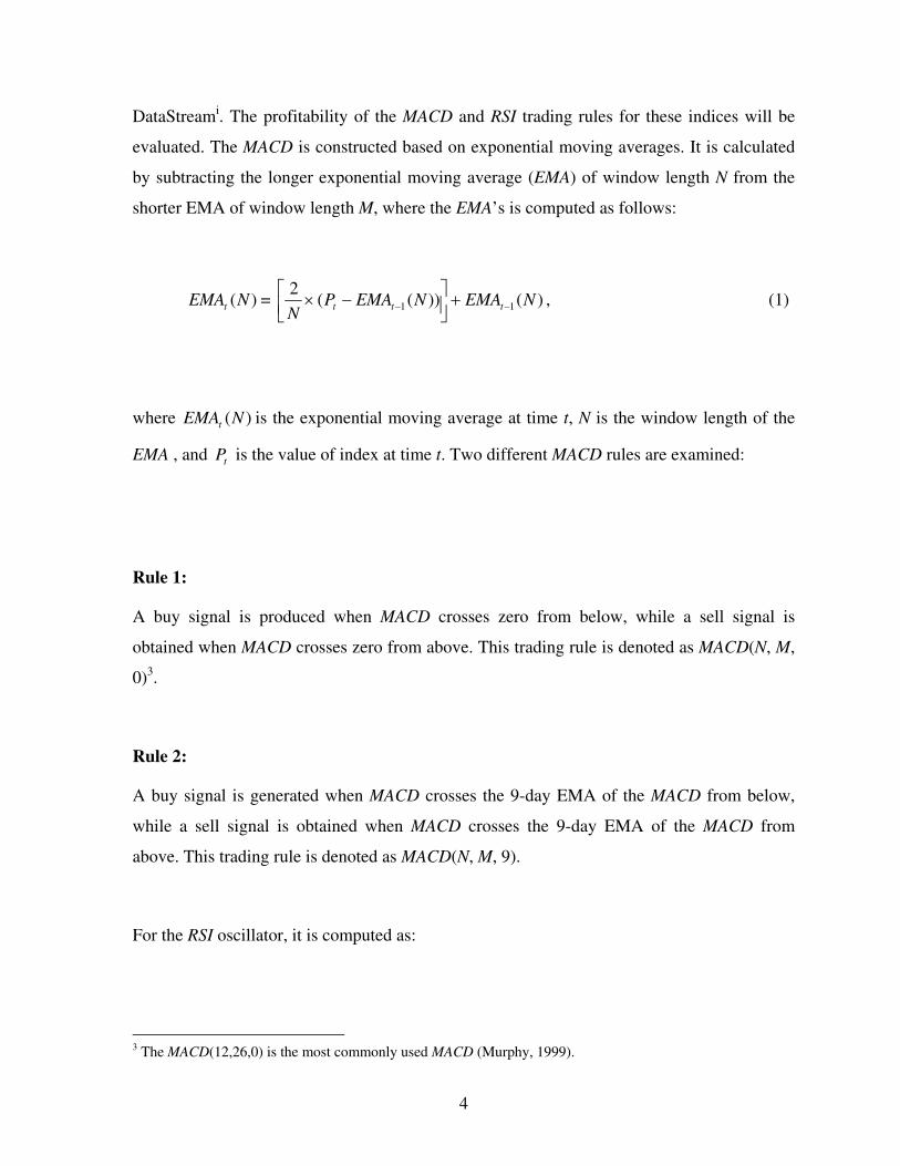
DataStreami. The profitability of the MACD and RSI trading rules for these indices will be

evaluated. The MACD is constructed based on exponential moving averages. It is calculated

by subtracting the longer exponential moving average (EMA) of window length N from the

shorter EMA of window length M, where the EMA’s is computed as follows:

)(NEMAt = )())((2

11 NEMANEMAPN

ttt

, (1)

where )(NEMAt is the exponential moving average at time t, N is the window length of the

EMA , and tP is the value of index at time t. Two different MACD rules are examined:

Rule 1:

A buy signal is produced when MACD crosses zero from below, while a sell signal is

obtained when MACD crosses zero from above. This trading rule is denoted as MACD(N, M,

0)3.

Rule 2:

A buy signal is generated when MACD crosses the 9-day EMA of the MACD from below,

while a sell signal is obtained when MACD crosses the 9-day EMA of the MACD from

above. This trading rule is denoted as MACD(N, M, 9).

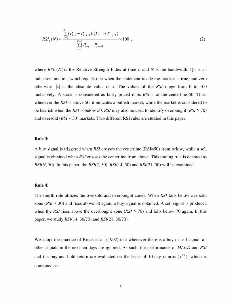
For the RSI oscillator, it is computed as:

3 The MACD(12,26,0) is the most commonly used MACD (Murphy, 1999).

5

100||

}{1)()(

1

01

1

0111

N

iitit

N

iittitit

t

PP

PPPP

NRSI , (2)

where )(NRSI t is the Relative Strength Index at time t, and N is the bandwidth. }{1 is an

indicator function, which equals one when the statement inside the bracket is true, and zero

otherwise. |x| is the absolute value of x. The values of the RSI range from 0 to 100

inclusively. A stock is considered as fairly priced if its RSI is at the centerline 50. Thus,

whenever the RSI is above 50, it indicates a bullish market, while the market is considered to

be bearish when the RSI is below 50. RSI may also be used to identify overbought (RSI > 70)

and oversold (RSI < 30) markets. Two different RSI rules are studied in this paper:

Rule 3:

A buy signal is triggered when RSI crosses the centerline (RSI=50) from below, while a sell

signal is obtained when RSI crosses the centerline from above. This trading rule is denoted as

RSI(N, 50). In this paper, the RSI(7, 50), RSI(14, 50) and RSI(21, 50) will be examined.

Rule 4:

The fourth rule utilizes the oversold and overbought zones. When RSI falls below oversold

zone (RSI < 30) and rises above 30 again, a buy signal is obtained. A sell signal is produced

when the RSI rises above the overbought zone (RSI > 70) and falls below 70 again. In this

paper, we study RSI(14, 30/70) and RSI(21, 30/70).

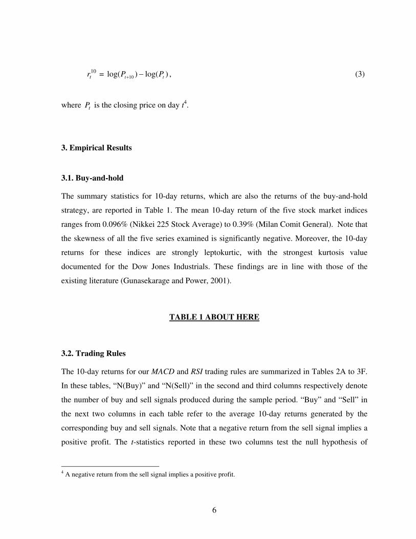
We adopt the practice of Brock et al. (1992) that whenever there is a buy or sell signal, all

other signals in the next ten days are ignored. As such, the performance of MACD and RSI

and the buy-and-hold return are evaluated on the basis of 10-day returns ( 10tr ), which is

computed as:

6

10tr = )log()log( 10 tt PP , (3)

where tP is the closing price on day t4.

3. Empirical Results

3.1. Buy-and-hold

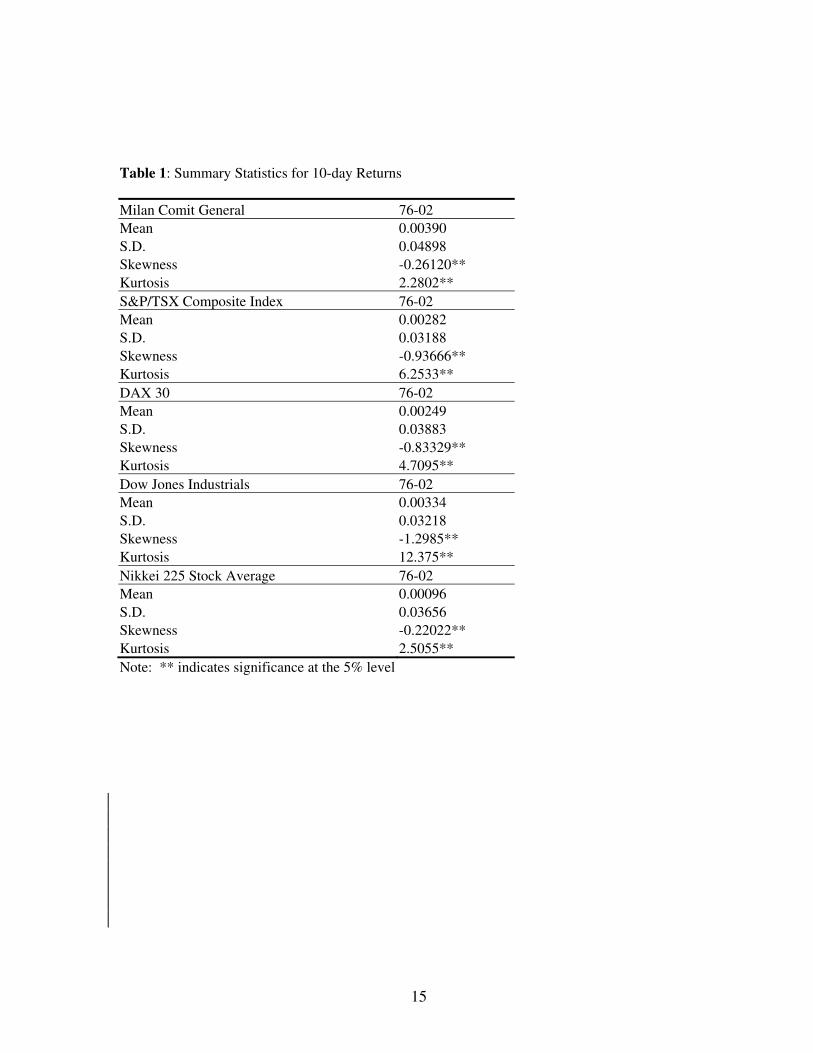
The summary statistics for 10-day returns, which are also the returns of the buy-and-hold

strategy, are reported in Table 1. The mean 10-day return of the five stock market indices

ranges from 0.096% (Nikkei 225 Stock Average) to 0.39% (Milan Comit General). Note that

the skewness of all the five series examined is significantly negative. Moreover, the 10-day

returns for these indices are strongly leptokurtic, with the strongest kurtosis value

documented for the Dow Jones Industrials. These findings are in line with those of the

existing literature (Gunasekarage and Power, 2001).

TABLE 1 ABOUT HERE

3.2. Trading Rules

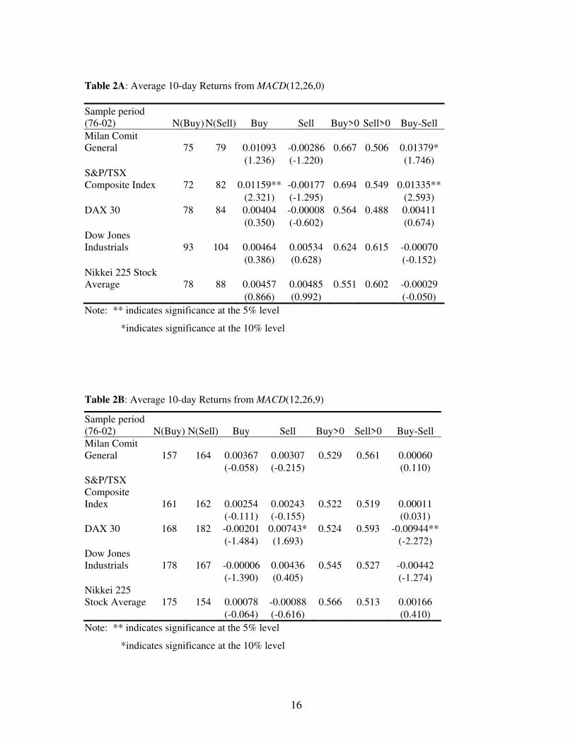
The 10-day returns for our MACD and RSI trading rules are summarized in Tables 2A to 3F.

In these tables, “N(Buy)” and “N(Sell)” in the second and third columns respectively denote

the number of buy and sell signals produced during the sample period. “Buy” and “Sell” in

the next two columns in each table refer to the average 10-day returns generated by the

corresponding buy and sell signals. Note that a negative return from the sell signal implies a

positive profit. The t-statistics reported in these two columns test the null hypothesis of

4 A negative return from the sell signal implies a positive profit.

7

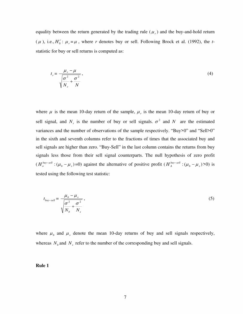
equality between the return generated by the trading rule ( r ) and the buy-and-hold return

( ), i.e., rH 0 : r = , where r denotes buy or sell. Following Brock et al. (1992), the t-

statistic for buy or sell returns is computed as:

rt =

NN r

r

22

, (4)

where is the mean 10-day return of the sample, r is the mean 10-day return of buy or

sell signal, and rN is the number of buy or sell signals. 2 and N are the estimated

variances and the number of observations of the sample respectively. “Buy>0” and “Sell>0”

in the sixth and seventh columns refer to the fractions of times that the associated buy and

sell signals are higher than zero. “Buy-Sell” in the last column contains the returns from buy

signals less those from their sell signal counterparts. The null hypothesis of zero profit

( )(: sb

sellbuy

oH =0) against the alternative of positive profit ( )(: sb

sellbuy

AH >0) is

tested using the following test statistic:

sellbuyt =

sb

sb

NN

22

, (5)

where b and s denote the mean 10-day returns of buy and sell signals respectively,

whereas bN and sN refer to the number of the corresponding buy and sell signals.

Rule 1

8

Table 2A summarizes the average 10-day return from the MACD(12,26,0) rule. The

MACD(12,26,0) rule performs well in the Milan Comit General and the S&P/TSX Composite

indices. The null hypothesis of the equality between returns from market indicators and the

buy-and-hold strategy is rejected at conventional significance levels. This suggests that the

trading strategy outperforms the buy-and-hold strategy. The most profitable buy (sell) signal

appears in the Milan Comit General index with an average 10-day return of 1.379%. Note

that the buy - sell returns are significantly positive. For the S&P/TSX Composite Index, both

the null hypotheses are rejected at the 5% significance level.

TABLE 2A ABOUT HERE

Rule 2

Table 2B shows the results of the MACD(12,26,9) rule. For Germany, the performance

of this rule is far from satisfactory. The rule is unable to yield a higher profit than the buy-

and-hold strategy. The buy – sell return is significantly negative at the 5% level, suggesting

that investors who follow the trading signals of MACD(12,26,9) will suffer a negative return

of 0.944% from a pair of buy and sell signals. The loss is sizeable compared to the positive

buy-and-hold return of 0.249%.

TABLE 2B ABOUT HERE

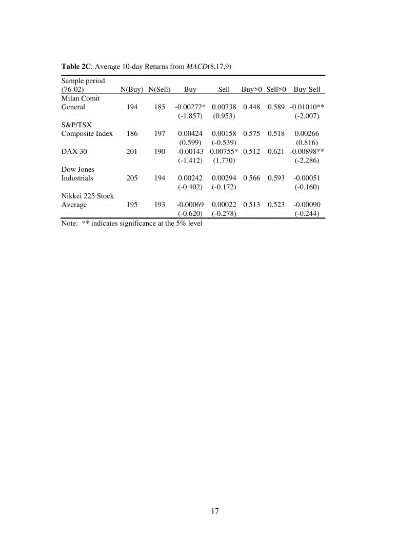
Among the five series examined, the trading rules perform the worst in the DAX 30.

For the remaining series, the MACD(12,26,9) has no predictability. As the combination of 8-

day, 17-day EMAs and signal line crossover can produce more reliable buy signals (Pring,

2002), we also examine the MACD(8,17,9) rule in this paper. From Table 2C, the return from

buy signals is negative for Italy. For Germany, the MACD(8,17,9) rule produces sell signals

which yield negative returns. The buy – sell returns are also significantly negative at the 5%

level for both countries.

9

TABLE 2C ABOUT HERE

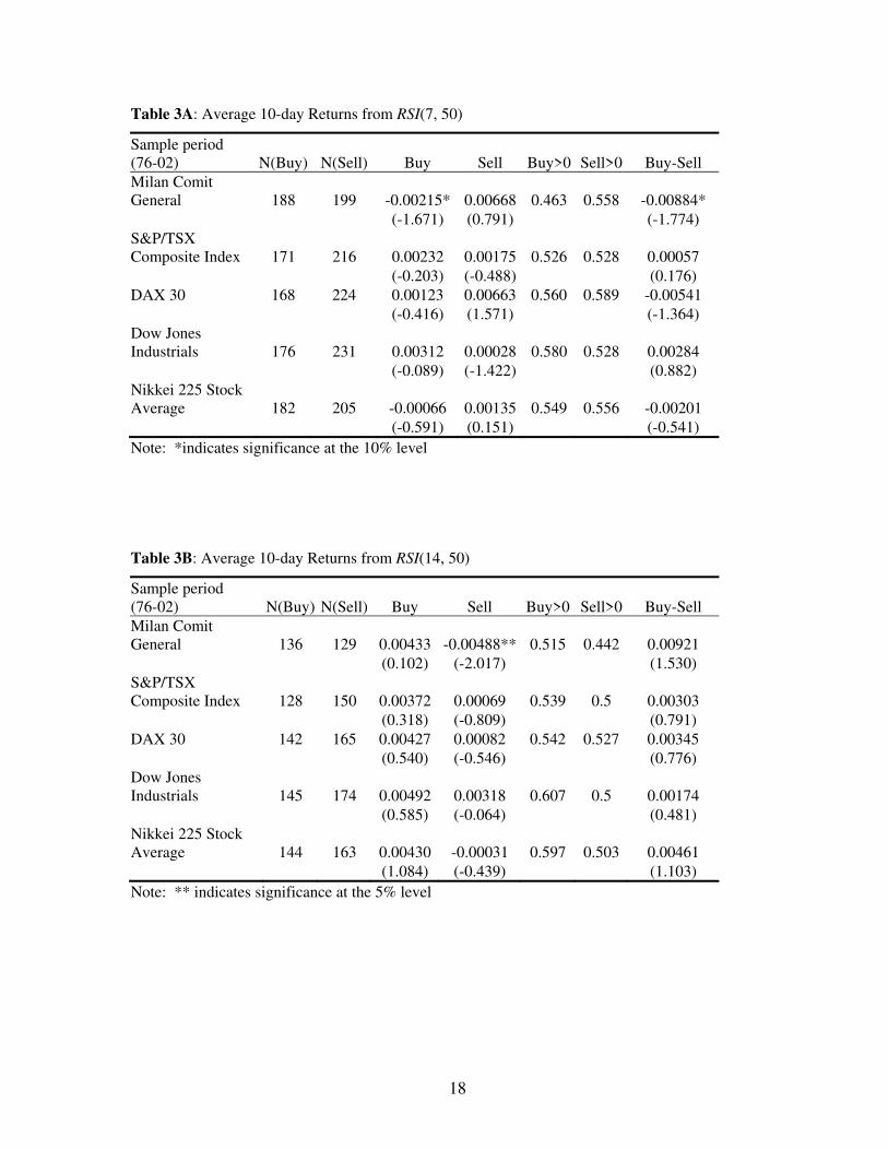
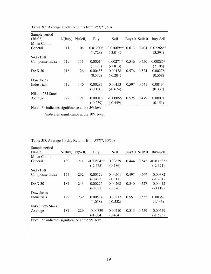
Rule 3

From Table 3A, the RSI(7,50) rule generates negative returns in the Milan Comit General.

The results in Table 3B indicate that the 14-day RSI rule has some predictability too. In

general, the buy-sell values are positive, implying that the rule is profitable. In most cases,

the RSI(14,50) rule is able to generate profits. The predictability of the trading rule for the

21-day RSI is reported in Table 3C. The rule beats the buy-and-hold strategy in the Milan

Comit General and the S&P / TSX Composite.

TABLE 3A ABOUT HERE

TABLE 3B ABOUT HERE

TABLE 3C ABOUT HERE

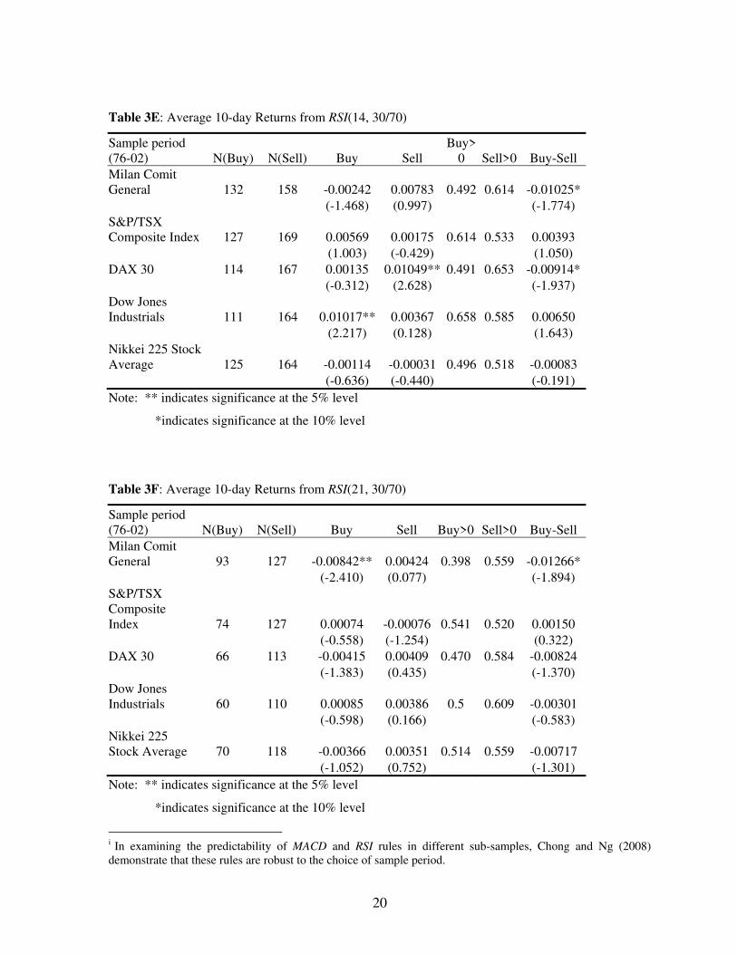
Rule 4

From Table 3D, most series have negative returns under the RSI(7, 30/70) rule. The return in

Milan Comit General is significantly negative. The loss is 1.163% from a pair of buy and sell

transactions. For other countries, none of the returns is significantly higher than the buy-and-

hold strategy. The RSI(14, 30/70) rule yields negative returns for three series. For the Milan

Comit General, a pair of buy and sell transactions generate a negative return of 1.03%, while

it is -0.91% for the DAX30. Note that the sell signal produces a significant loss of 1.049%

for the DAX30. However, the rule slightly outperforms the buy-and-hold strategy in the Dow

Jones Industrials. For all other rules, no significant return is found. The RSI(21, 30/70) rule

generates a negative return for the Milan Comit General.

10

TABLE 3D ABOUT HERE

3.3 Transaction Cost

The above results are obtained in the absence of transaction costs. In this section, we relax

this assumption. According to the survey of Hudson et al. (1996) on stockbrokers and stock

broking divisions of major clearing banks, the minimum commission fee is at least 0.1%.

When the bid-offer spreads of 0.5% and government stamp duty of 0.5% are included, the

round-trip transaction cost is at least 1%.5 They show that technical trading rules of Brock et

al. (1992) do not generate excess returns in the UK market after taking a round-trip

transaction cost of 1% into consideration. Mills (1997) also shows that the moving average

and trading range breakout rules cannot produce returns higher than the buy-and-hold

strategy when a 1% transaction cost is taken into account. Therefore, in this paper, a 1%

transaction cost is included to compute the net profits from each of the trading rule6. We will

focus on the Italian and Canadian markets, which contain the largest number of profitable

trading rules. It is found that in the presence of a 1% transaction cost, the MACD(12,26,0)

applied to these two countries are still profitable. For Milan Comit General index and S&P /

TSX Composite index, the net profits of the MACD(12,26,0) rule are 1.021%7 and 0.776%

respectively. Moreover, the average annual return of the RSI(21,50) rule net of a 1% round-

trip transaction cost for the Milan Comit General index is 5.069%.

4. Conclusion

The discipline of finance has been dominated by the Efficient Market Hypothesis (EMH) for

four decades since the pioneering work of Fama (1970). However, the EMH is built under

5 Due to the increasing competition among stock brokers and the introduction of internet trading, transaction costs have been reduced sharply in recent years. It is expected that the trend of this reduction in transaction cost will continue, which will provide more room for the development of technical trading rules in the future. 6 Rouwenhorst (1998) points out that for the large and liquid stock markets in Europe, the transaction cost is less than 1%. 7 Note that there are 75 buy signals and 79 sell signals over the 27-year period. Therefore, the annual return net of transaction cost is (1.093%-0.5%)*75/27+(0.286%-0.5%)*79/27=1.021%.

11

the very assumptions that investors are rational and fully informed. If technical analysis can

yield abnormal returns, it implies that the EMH and its underlying assumptions fail to hold.

In recent years, researchers have attempted to identify profitable trading rules resulting from

patterns of human behavior. This study contributes to the existing literature of behavioral

finance by reporting the profitability of two oscillators, namely the Moving Average

Convergence-Divergence (MACD) and Relative Strength Index (RSI) in five major OECD

markets. The two rules have been widely used by investors but their empirical performance is

relatively unexplored.

This study finds that the centerline crossover of the RSI has predictive ability in the Italian

and Canadian stock markets. In particular, the RSI(21,50) rule performs well in the Milan

Comit General index. The RSI(14,30/70) rule is also profitable in the Dow Jones Industrials

index. The profits are sustainable in the presence of a 1% round-trip transaction cost. These

findings are in line with Chong and Ng (2008) that the MACD and RSI rules can generate

significant profit for FT30. However, for the Nikkei 225 Stock Average, none of the rules

can beat the buy-and-hold strategy. When the two rules of RSI are compared, it is found that

the performance of centreline line crossover is better. Our results shed some light on

investors’ believe in these two technical indicators in different developed markets. The

presence of trading rule profits also indicates that investors in these markets may only be

boundedly rational.

Notably, Chong and Ng (2008) demonstrate that MACD and RSI rules are robust to the

choice of sample. However, it is important to note that the current study finds that these rules

are not robust to the choice of market. Taking these findings together, before adopting these

rules, it is advisable for traders and practitioners to at least ascertain the profitability of these

rules in their markets using historical data. In addition, a simulation trading portfolio could

be created in order to discover the full potential of these indicators under a real situation. 8

Moreover, practitioners or academics may examine the profitability of these rules for

individual shares as an extension to the spirit of this study.

8 We thank an anonymous referee for giving us this suggestion.

12

References

Allen, F. and R. Karjalainen, 1999. Using genetic algorithms to find technical trading rules.

Journal of Financial Economics 51, 245-271.

Bessembinder, H. and K. Chan, 1995. The profitability of technical rules in the Asian stock

markets. Pacific-Basin Finance Journal 3, 257 - 284.

Brock, W., J. Lakonishok and B. LeBaron, 1992. Simple technical trading rules and the

stochastic properties of stock returns. Journal of Finance 5, 1731-1764.

Chen, H., T. T. L. Chong and X. Duan, 2010. A principal-component approach to measuring

investor sentiment. Quantitative Finance 10(4), 339-347.

Chong, T. T. L. and H. Ip, 2009. Do momentum-based strategies work in emerging currency markets? Pacific-Basin Finance Journal 17, 479-493.

Chong, T. T. L. and W. K. Ng. 2008. Technical analysis and the London stock exchange:

testing the MACD and RSI rules using the FT30. Applied Economics Letters 15, 1111-

1114.

Fama, E. F., 1970. Efficient capital market, a review of theory and empirical work. Journal

of Finance 25, 383- 417.

Gunasekarage, A. and D. M. Power, 2001. The profitability of moving average trading rules

in South Asian stock markets. Emerging Market Review 2, 17 - 33.

Hudson, R., M. Dempsey and K. Keasey, 1996. A note on the weak form efficiency of

capital markets: The application of simple technical trading rules to UK stock prices —

1935 to 1994. Journal of Banking and Finance 20, 1121-1132.

13

Jensen, M. C. and G. A. Benington, 1970. Random walk and technical theories: some

additional evidence. Journal of Finance 25, 469 - 482.

Kwon, K. Y. and R. J. Kish. 2002. Technical trading strategies and return predictability:

NYSE. Applied Financial Economics 12, 639-653.

Lui, K. M. and T. T. L. Chong, 2013. Do technical analysts outperform novice traders: Experimental evidence. Economics Bulletin 33(4), 3080-3087.

Mills, T. C., 1997. Technical analysis and the London Stock Exchange: Testing trading rules

using the FT30. International Journal of Finance and Economics 2, 319-331.

Murphy, J. J., 1999. Technical Analysis of the Financial Markets: A Comprehensive Guide to

Trading Methods and Applications, New York Institute of Finance.

Neftçi, S. N., 1991. Naïve trading rules in financial markets and Wiener-Kolmogorov

prediction theory: A study of “technical analysis”. Journal of Business 64, 549-571.

Ni, H. and H. Yin. 2009. Exchange rate prediction using hybrid neural networks and trading

indicators. Neurocomputing 72, 2815-2823.

Pring, M. J., 2002. Momentum Explained, Volume 1 & 2, McGraw-Hill, New York.

Rosillo, R,; D. de la Fuente and J. A. L. Brugos. 2013. Technical analysis and the Spanish

stock exchange: testing the RSI, MACD, momentum and stochastic rules using Spanish

market companies. Applied Economics 45(12), 1541 -1550.Rouwenhorst, K.G., 1998.

International momentum strategies. Journal of Finance 53, 267-284.

Stawicki, S. P. 2007. Application of financial analysis techniques to vital sign data: a novel

method of trend interpretation in the intensive care unit. OPUS12 Scientist 1, 14-16.

14

Sullivan, R., A. Timmerman and H. White, 1999. Data-snooping, technical trading rule

performance and the Bootstrap, Journal of Finance 54, 1647-1691.

Tanaka-Yamawaki, M. and S. Tokuoka. 2007. Adaptive use of technical indicators for the

prediction of intra-day stock prices. Physica A 383, 125-133.

Timmermann, A. and C.W.J. Granger, 2004. Efficient market hypothesis and forecasting.

International Journal of Forecasting 20, 15– 27.

Treynor, J. L. and R. Ferguson, 1985. In defense of technical analysis. Journal of Finance

40, 757-773.

Ülkü, N. and E. Prodan, 2013. Drivers of technical trend-following rules' profitability in

world stock markets. International Review of Financial Analysis 30 (2013) 214–229.

White, R. 2013. Technical Analysis Indicator That Works Turns Positive For These Stocks,

Forbes, April 15, 2013. Available at:

http://www.forbes.com/sites/greatspeculations/2013/04/15/technical-analysis-indicator-

that-works-turns-positive-for-these-stocks/. Accessed: Dec 27, 2013.

Wilder, J. W. 1978. New Concepts in Technical Trading Systems. USA: Trend Research.

15

Table 1: Summary Statistics for 10-day Returns

Milan Comit General 76-02 Mean 0.00390 S.D. 0.04898 Skewness -0.26120** Kurtosis 2.2802** S&P/TSX Composite Index 76-02 Mean 0.00282 S.D. 0.03188 Skewness -0.93666** Kurtosis 6.2533** DAX 30 76-02 Mean 0.00249 S.D. 0.03883 Skewness -0.83329** Kurtosis 4.7095** Dow Jones Industrials 76-02 Mean 0.00334 S.D. 0.03218 Skewness -1.2985** Kurtosis 12.375** Nikkei 225 Stock Average 76-02 Mean 0.00096 S.D. 0.03656 Skewness -0.22022** Kurtosis 2.5055** Note: ** indicates significance at the 5% level

16

Table 2A: Average 10-day Returns from MACD(12,26,0)

Sample period (76-02) N(Buy) N(Sell) Buy Sell Buy>0 Sell>0 Buy-Sell Milan Comit General 75 79 0.01093 -0.00286 0.667 0.506 0.01379* (1.236) (-1.220) (1.746) S&P/TSX Composite Index 72 82 0.01159** -0.00177 0.694 0.549 0.01335** (2.321) (-1.295) (2.593) DAX 30 78 84 0.00404 -0.00008 0.564 0.488 0.00411 (0.350) (-0.602) (0.674) Dow Jones Industrials 93 104 0.00464 0.00534 0.624 0.615 -0.00070 (0.386) (0.628) (-0.152) Nikkei 225 Stock Average 78 88 0.00457 0.00485 0.551 0.602 -0.00029 (0.866) (0.992) (-0.050) Note: ** indicates significance at the 5% level

*indicates significance at the 10% level

Table 2B: Average 10-day Returns from MACD(12,26,9)

Sample period (76-02) N(Buy) N(Sell) Buy Sell Buy>0 Sell>0 Buy-Sell Milan Comit General 157 164 0.00367 0.00307 0.529 0.561 0.00060 (-0.058) (-0.215) (0.110) S&P/TSX Composite Index 161 162 0.00254 0.00243 0.522 0.519 0.00011 (-0.111) (-0.155) (0.031) DAX 30 168 182 -0.00201 0.00743* 0.524 0.593 -0.00944** (-1.484) (1.693) (-2.272) Dow Jones Industrials 178 167 -0.00006 0.00436 0.545 0.527 -0.00442 (-1.390) (0.405) (-1.274) Nikkei 225 Stock Average 175 154 0.00078 -0.00088 0.566 0.513 0.00166 (-0.064) (-0.616) (0.410) Note: ** indicates significance at the 5% level

*indicates significance at the 10% level

17

Table 2C: Average 10-day Returns from MACD(8,17,9)

Sample period (76-02) N(Buy) N(Sell) Buy Sell Buy>0 Sell>0 Buy-Sell Milan Comit General 194 185 -0.00272* 0.00738 0.448 0.589 -0.01010** (-1.857) (0.953) (-2.007) S&P/TSX Composite Index 186 197 0.00424 0.00158 0.575 0.518 0.00266 (0.599) (-0.539) (0.816) DAX 30 201 190 -0.00143 0.00755* 0.512 0.621 -0.00898** (-1.412) (1.770) (-2.286) Dow Jones Industrials 205 194 0.00242 0.00294 0.566 0.593 -0.00051 (-0.402) (-0.172) (-0.160) Nikkei 225 Stock Average 195 193 -0.00069 0.00022 0.513 0.523 -0.00090 (-0.620) (-0.278) (-0.244) Note: ** indicates significance at the 5% level

18

Table 3A: Average 10-day Returns from RSI(7, 50)

Sample period (76-02) N(Buy) N(Sell) Buy Sell Buy>0 Sell>0 Buy-Sell Milan Comit General 188 199 -0.00215* 0.00668 0.463 0.558 -0.00884* (-1.671) (0.791) (-1.774) S&P/TSX Composite Index 171 216 0.00232 0.00175 0.526 0.528 0.00057 (-0.203) (-0.488) (0.176) DAX 30 168 224 0.00123 0.00663 0.560 0.589 -0.00541 (-0.416) (1.571) (-1.364) Dow Jones Industrials 176 231 0.00312 0.00028 0.580 0.528 0.00284 (-0.089) (-1.422) (0.882) Nikkei 225 Stock Average 182 205 -0.00066 0.00135 0.549 0.556 -0.00201 (-0.591) (0.151) (-0.541) Note: *indicates significance at the 10% level

Table 3B: Average 10-day Returns from RSI(14, 50)

Sample period (76-02) N(Buy) N(Sell) Buy Sell Buy>0 Sell>0 Buy-Sell Milan Comit General 136 129 0.00433 -0.00488** 0.515 0.442 0.00921 (0.102) (-2.017) (1.530) S&P/TSX Composite Index 128 150 0.00372 0.00069 0.539 0.5 0.00303 (0.318) (-0.809) (0.791) DAX 30 142 165 0.00427 0.00082 0.542 0.527 0.00345 (0.540) (-0.546) (0.776) Dow Jones Industrials 145 174 0.00492 0.00318 0.607 0.5 0.00174 (0.585) (-0.064) (0.481) Nikkei 225 Stock Average 144 163 0.00430 -0.00031 0.597 0.503 0.00461 (1.084) (-0.439) (1.103) Note: ** indicates significance at the 5% level

19

Table 3C: Average 10-day Returns from RSI(21, 50)

Sample period (76-02) N(Buy) N(Sell) Buy Sell Buy>0 Sell>0 Buy-Sell Milan Comit General 111 104 0.01200* -0.01069** 0.613 0.404 0.02268** (1.728) (-3.014) (3.394) S&P/TSX Composite Index 119 111 0.00614 -0.00271* 0.546 0.450 0.00885* (1.127) (-1.813) (2.105) DAX 30 118 126 0.00455 0.00178 0.576 0.524 0.00278 (0.572) (-0.204) (0.558) Dow Jones Industrials 119 146 0.00287 0.00153 0.597 0.541 0.00134 (-0.160) (-0.674) (0.337) Nikkei 225 Stock Average 122 121 0.00016 -0.00055 0.525 0.479 0.00071 (-0.239) (-0.449) (0.151) Note: ** indicates significance at the 5% level

*indicates significance at the 10% level

Table 3D: Average 10-day Returns from RSI(7, 30/70)

Sample period (76-02) N(Buy) N(Sell) Buy Sell Buy>0 Sell>0 Buy-Sell Milan Comit General 189 211 -0.00504** 0.00659 0.444 0.545 -0.01163** (-2.475) (0.786) (-2.371) S&P/TSX Composite Index 177 232 0.00179 0.00561 0.497 0.569 -0.00382 (-0.425) (1.311) (-1.201) DAX 30 187 243 0.00226 0.00268 0.540 0.527 -0.00042 (-0.081) (0.076) (-0.112) Dow Jones Industrials 192 239 0.00574 0.00217 0.557 0.552 0.00357 (1.018) (-0.552) (1.143) Nikkei 225 Stock Average 187 229 -0.00339 0.00210 0.513 0.559 -0.00549 (-1.604) (0.464) (-1.523) Note: ** indicates significance at the 5% level

20

Table 3E: Average 10-day Returns from RSI(14, 30/70)

Sample period (76-02) N(Buy) N(Sell) Buy Sell

Buy>0 Sell>0 Buy-Sell

Milan Comit General 132 158 -0.00242 0.00783 0.492 0.614 -0.01025* (-1.468) (0.997) (-1.774) S&P/TSX Composite Index 127 169 0.00569 0.00175 0.614 0.533 0.00393 (1.003) (-0.429) (1.050) DAX 30 114 167 0.00135 0.01049** 0.491 0.653 -0.00914* (-0.312) (2.628) (-1.937) Dow Jones Industrials 111 164 0.01017** 0.00367 0.658 0.585 0.00650 (2.217) (0.128) (1.643) Nikkei 225 Stock Average 125 164 -0.00114 -0.00031 0.496 0.518 -0.00083 (-0.636) (-0.440) (-0.191) Note: ** indicates significance at the 5% level

*indicates significance at the 10% level

Table 3F: Average 10-day Returns from RSI(21, 30/70)

Sample period (76-02) N(Buy) N(Sell) Buy Sell Buy>0 Sell>0 Buy-Sell Milan Comit General 93 127 -0.00842** 0.00424 0.398 0.559 -0.01266* (-2.410) (0.077) (-1.894) S&P/TSX Composite Index 74 127 0.00074 -0.00076 0.541 0.520 0.00150 (-0.558) (-1.254) (0.322) DAX 30 66 113 -0.00415 0.00409 0.470 0.584 -0.00824 (-1.383) (0.435) (-1.370) Dow Jones Industrials 60 110 0.00085 0.00386 0.5 0.609 -0.00301 (-0.598) (0.166) (-0.583) Nikkei 225 Stock Average 70 118 -0.00366 0.00351 0.514 0.559 -0.00717 (-1.052) (0.752) (-1.301) Note: ** indicates significance at the 5% level

*indicates significance at the 10% level

i In examining the predictability of MACD and RSI rules in different sub-samples, Chong and Ng (2008) demonstrate that these rules are robust to the choice of sample period.