Revisiting Unreasonable Effectiveness of Data in Deep Learning Era

Chen Sun1, Abhinav Shrivastava1,2, Saurabh Singh1, and Abhinav Gupta1,2

1Google Research2Carnegie Mellon University

Abstract

The success of deep learning in vision can be attributedto: (a) models with high capacity; (b) increased compu-tational power; and (c) availability of large-scale labeleddata. Since 2012, there have been significant advances inrepresentation capabilities of the models and computationalcapabilities of GPUs. But the size of the biggest dataset hassurprisingly remained constant. What will happen if we in-crease the dataset size by 10× or 100×? This paper takesa step towards clearing the clouds of mystery surroundingthe relationship between ‘enormous data’ and visual deeplearning. By exploiting the JFT-300M dataset which hasmore than 375M noisy labels for 300M images, we inves-tigate how the performance of current vision tasks wouldchange if this data was used for representation learning.Our paper delivers some surprising (and some expected)findings. First, we find that the performance on vision tasksincreases logarithmically based on volume of training datasize. Second, we show that representation learning (or pre-training) still holds a lot of promise. One can improve per-formance on many vision tasks by just training a better basemodel. Finally, as expected, we present new state-of-the-art results for different vision tasks including image clas-sification, object detection, semantic segmentation and hu-man pose estimation. Our sincere hope is that this inspiresvision community to not undervalue the data and developcollective efforts in building larger datasets.

1. Introduction

There is unanimous agreement that the current ConvNetrevolution is a product of big labeled datasets (specifically,1M labeled images from ImageNet [35]) and large compu-tational power (thanks to GPUs). Every year we get furtherincrease in computational power (a newer and faster GPU)but our datasets have not been so fortunate. ImageNet, adataset of 1M labeled images based on 1000 categories, wasused to train AlexNet [25] more than five years ago. Curi-

150

300

AlexNetVGG

ResNet-50

ResNet-101

Inception ResNet-v2

# Paramaters

6000

12000

2012 2013 2014 2015 2016

GFl

ops

# of

Lay

ers

# of

Imag

es (M

)

1

1.5 Dataset Size

Model Size

GPU Power

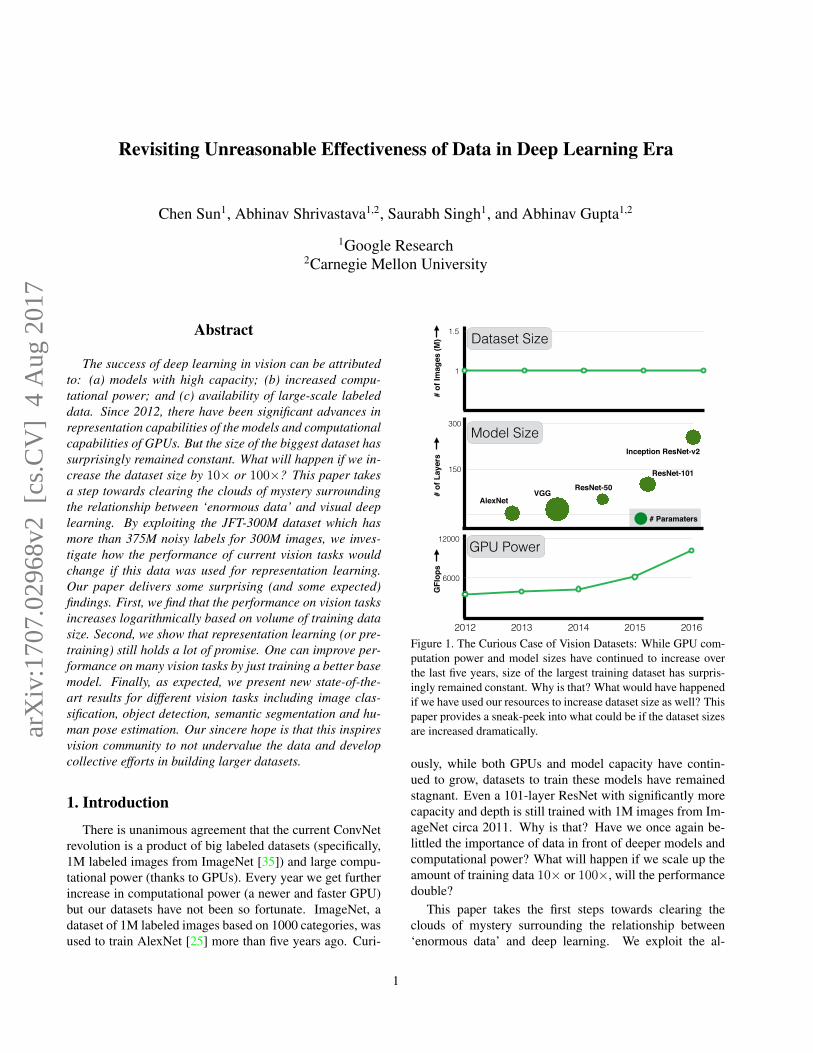
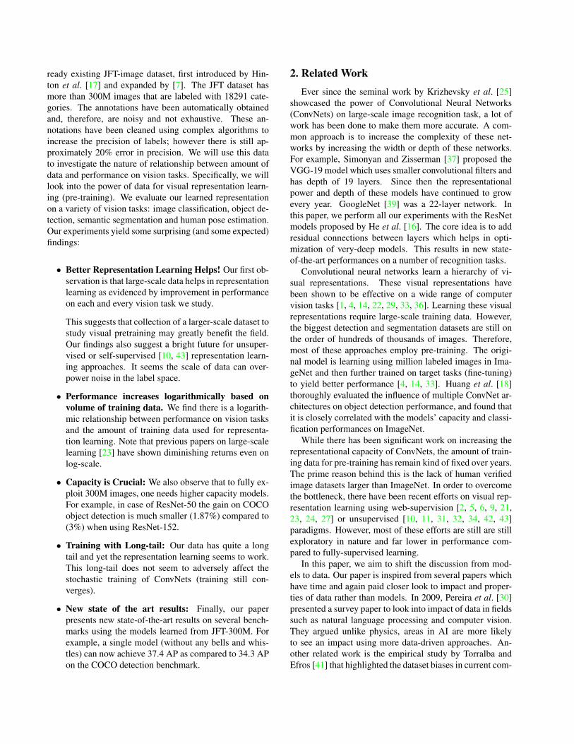
Figure 1. The Curious Case of Vision Datasets: While GPU com-putation power and model sizes have continued to increase overthe last five years, size of the largest training dataset has surpris-ingly remained constant. Why is that? What would have happenedif we have used our resources to increase dataset size as well? Thispaper provides a sneak-peek into what could be if the dataset sizesare increased dramatically.

ously, while both GPUs and model capacity have contin-ued to grow, datasets to train these models have remainedstagnant. Even a 101-layer ResNet with significantly morecapacity and depth is still trained with 1M images from Im-ageNet circa 2011. Why is that? Have we once again be-littled the importance of data in front of deeper models andcomputational power? What will happen if we scale up theamount of training data 10× or 100×, will the performancedouble?

This paper takes the first steps towards clearing theclouds of mystery surrounding the relationship between‘enormous data’ and deep learning. We exploit the al-

1

arX

iv:1

707.

0296

8v2

[cs

.CV

] 4

Aug

201

7

ready existing JFT-image dataset, first introduced by Hin-ton et al. [17] and expanded by [7]. The JFT dataset hasmore than 300M images that are labeled with 18291 cate-gories. The annotations have been automatically obtainedand, therefore, are noisy and not exhaustive. These an-notations have been cleaned using complex algorithms toincrease the precision of labels; however there is still ap-proximately 20% error in precision. We will use this datato investigate the nature of relationship between amount ofdata and performance on vision tasks. Specifically, we willlook into the power of data for visual representation learn-ing (pre-training). We evaluate our learned representationon a variety of vision tasks: image classification, object de-tection, semantic segmentation and human pose estimation.Our experiments yield some surprising (and some expected)findings:

• Better Representation Learning Helps! Our first ob-servation is that large-scale data helps in representationlearning as evidenced by improvement in performanceon each and every vision task we study.

This suggests that collection of a larger-scale dataset tostudy visual pretraining may greatly benefit the field.Our findings also suggest a bright future for unsuper-vised or self-supervised [10, 43] representation learn-ing approaches. It seems the scale of data can over-power noise in the label space.

• Performance increases logarithmically based onvolume of training data. We find there is a logarith-mic relationship between performance on vision tasksand the amount of training data used for representa-tion learning. Note that previous papers on large-scalelearning [23] have shown diminishing returns even onlog-scale.

• Capacity is Crucial: We also observe that to fully ex-ploit 300M images, one needs higher capacity models.For example, in case of ResNet-50 the gain on COCOobject detection is much smaller (1.87%) compared to(3%) when using ResNet-152.

• Training with Long-tail: Our data has quite a longtail and yet the representation learning seems to work.This long-tail does not seem to adversely affect thestochastic training of ConvNets (training still con-verges).

• New state of the art results: Finally, our paperpresents new state-of-the-art results on several bench-marks using the models learned from JFT-300M. Forexample, a single model (without any bells and whis-tles) can now achieve 37.4 AP as compared to 34.3 APon the COCO detection benchmark.

2. Related WorkEver since the seminal work by Krizhevsky et al. [25]

showcased the power of Convolutional Neural Networks(ConvNets) on large-scale image recognition task, a lot ofwork has been done to make them more accurate. A com-mon approach is to increase the complexity of these net-works by increasing the width or depth of these networks.For example, Simonyan and Zisserman [37] proposed theVGG-19 model which uses smaller convolutional filters andhas depth of 19 layers. Since then the representationalpower and depth of these models have continued to growevery year. GoogleNet [39] was a 22-layer network. Inthis paper, we perform all our experiments with the ResNetmodels proposed by He et al. [16]. The core idea is to addresidual connections between layers which helps in opti-mization of very-deep models. This results in new state-of-the-art performances on a number of recognition tasks.

Convolutional neural networks learn a hierarchy of vi-sual representations. These visual representations havebeen shown to be effective on a wide range of computervision tasks [1, 4, 14, 22, 29, 33, 36]. Learning these visualrepresentations require large-scale training data. However,the biggest detection and segmentation datasets are still onthe order of hundreds of thousands of images. Therefore,most of these approaches employ pre-training. The origi-nal model is learning using million labeled images in Ima-geNet and then further trained on target tasks (fine-tuning)to yield better performance [4, 14, 33]. Huang et al. [18]thoroughly evaluated the influence of multiple ConvNet ar-chitectures on object detection performance, and found thatit is closely correlated with the models’ capacity and classi-fication performances on ImageNet.

While there has been significant work on increasing therepresentational capacity of ConvNets, the amount of train-ing data for pre-training has remain kind of fixed over years.The prime reason behind this is the lack of human verifiedimage datasets larger than ImageNet. In order to overcomethe bottleneck, there have been recent efforts on visual rep-resentation learning using web-supervision [2, 5, 6, 9, 21,23, 24, 27] or unsupervised [10, 11, 31, 32, 34, 42, 43]paradigms. However, most of these efforts are still are stillexploratory in nature and far lower in performance com-pared to fully-supervised learning.

In this paper, we aim to shift the discussion from mod-els to data. Our paper is inspired from several papers whichhave time and again paid closer look to impact and proper-ties of data rather than models. In 2009, Pereira et al. [30]presented a survey paper to look into impact of data in fieldssuch as natural language processing and computer vision.They argued unlike physics, areas in AI are more likelyto see an impact using more data-driven approaches. An-other related work is the empirical study by Torralba andEfros [41] that highlighted the dataset biases in current com-

puter vision approaches and how it impacts future research.Specifically, we focus on understanding the relationship

between data and visual deep learning. There have beensome efforts to understand this relationship. For example,Oquab et al. [28] showed that expanding the training datato cover 1512 labels from ImageNet-14M further improvesthe object detection performance. Similarly, Huh et al. [19]showed that using a smaller subset of images for trainingfrom ImageNet hurts performance. Both these studies alsoshow that selection of categories for training is importantand random addition of categories tends to hurt the perfor-mance. But what happens when the number of categoriesare increased 10x? Do we still need manual selection ofcategories? Similarly, neither of these efforts demonstrateddata effects at significantly larger scale.

Some recent work [23, 44] have looked at training Con-vNets with significantly larger data. While [44] looked atgeo-localization, [23] utilized the YFCC-100M dataset [40]for representation learning. However, unlike ours, [23]showed plateauing of detection performance when trainedon 100M images. Why is that? We believe there could betwo possible reasons: a) YFCC-100M images come onlyfrom Flickr. JFT includes images all over the web, and hasbetter visual diversity. The usage of user feedback signalsin JFT further reduces label noise. YFCC-100M has a muchbigger vocabulary size and noisier annotations. b) But moreimportantly, they did not see real effect of data due to use ofsmaller AlexNet of VGG models. In our experiments, wesee more gain with larger model sizes.

3. The JFT-300M DatasetWe now introduce the JFT-300M dataset used through-

out this paper. JFT-300M is a follow up version of thedataset introduced by [7, 17]. The JFT-300M dataset isclosely related and derived from the data which powers theImage Search. In this version, the dataset has 300M imagesand 375M labels, on average each image has 1.26 labels.These images are labeled with 18291 categories: e.g., 1165type of animals and 5720 types of vehicles are labeled inthe dataset. These categories form a rich hierarchy with themaximum depth of hierarchy being 12 and maximum num-ber of child for parent node being 2876.

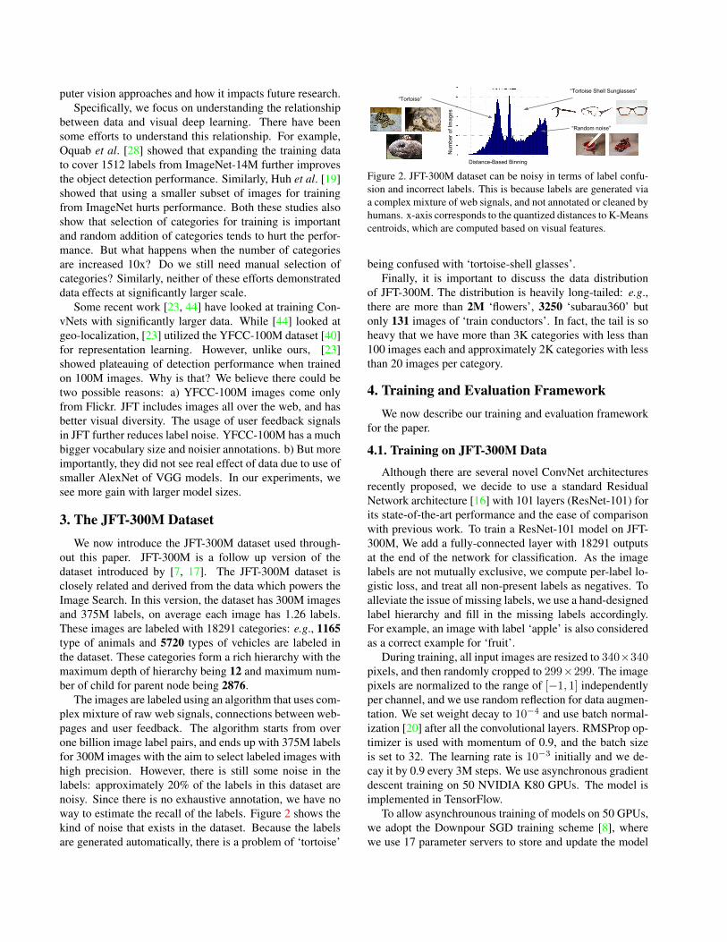
The images are labeled using an algorithm that uses com-plex mixture of raw web signals, connections between web-pages and user feedback. The algorithm starts from overone billion image label pairs, and ends up with 375M labelsfor 300M images with the aim to select labeled images withhigh precision. However, there is still some noise in thelabels: approximately 20% of the labels in this dataset arenoisy. Since there is no exhaustive annotation, we have noway to estimate the recall of the labels. Figure 2 shows thekind of noise that exists in the dataset. Because the labelsare generated automatically, there is a problem of ‘tortoise’

Distance-Based Binning

“Tortoise”“Tortoise Shell Sunglasses”

“Random noise”

Num

ber o

f Im

ages

Figure 2. JFT-300M dataset can be noisy in terms of label confu-sion and incorrect labels. This is because labels are generated viaa complex mixture of web signals, and not annotated or cleaned byhumans. x-axis corresponds to the quantized distances to K-Meanscentroids, which are computed based on visual features.

being confused with ‘tortoise-shell glasses’.Finally, it is important to discuss the data distribution

of JFT-300M. The distribution is heavily long-tailed: e.g.,there are more than 2M ‘flowers’, 3250 ‘subarau360’ butonly 131 images of ‘train conductors’. In fact, the tail is soheavy that we have more than 3K categories with less than100 images each and approximately 2K categories with lessthan 20 images per category.

4. Training and Evaluation FrameworkWe now describe our training and evaluation framework

for the paper.

4.1. Training on JFT-300M Data

Although there are several novel ConvNet architecturesrecently proposed, we decide to use a standard ResidualNetwork architecture [16] with 101 layers (ResNet-101) forits state-of-the-art performance and the ease of comparisonwith previous work. To train a ResNet-101 model on JFT-300M, We add a fully-connected layer with 18291 outputsat the end of the network for classification. As the imagelabels are not mutually exclusive, we compute per-label lo-gistic loss, and treat all non-present labels as negatives. Toalleviate the issue of missing labels, we use a hand-designedlabel hierarchy and fill in the missing labels accordingly.For example, an image with label ‘apple’ is also consideredas a correct example for ‘fruit’.

During training, all input images are resized to 340×340pixels, and then randomly cropped to 299×299. The imagepixels are normalized to the range of [−1, 1] independentlyper channel, and we use random reflection for data augmen-tation. We set weight decay to 10−4 and use batch normal-ization [20] after all the convolutional layers. RMSProp op-timizer is used with momentum of 0.9, and the batch sizeis set to 32. The learning rate is 10−3 initially and we de-cay it by 0.9 every 3M steps. We use asynchronous gradientdescent training on 50 NVIDIA K80 GPUs. The model isimplemented in TensorFlow.

To allow asynchrounous training of models on 50 GPUs,we adopt the Downpour SGD training scheme [8], wherewe use 17 parameter servers to store and update the model

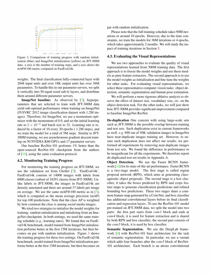
Figure 3. Comparison of training progress with random initial-ization (blue) and ImageNet initialization (yellow) on JFT-300Mdata. x-axis is the number of training steps, and y-axis shows themAP@100 metric computed on FastEval14k.

weights. The final classification fully-connected layer with2048 input units and over 18K output units has over 36Mparameters. To handle this in our parameter servers, we splitit vertically into 50 equal sized sub-fc layers, and distributethem around different parameter servers.

ImageNet baseline: As observed by [7], hyperpa-rameters that are selected to train with JFT-300M datayield sub-optimal performance when training on ImageNet(IVSVRC 2012 image classification dataset with 1.2M im-ages). Therefore, for ImageNet, we use a momentum opti-mizer with the momentum of 0.9, and set the initial learningrate to 5 × 10−2 and batch size to 32. Learning rate is re-duced by a factor of 10 every 30 epochs ( 1.2M steps), andwe train the model for a total of 5M steps. Similar to JFT-300M training, we use asynchronous gradient descent train-ing on 50 NVIDIA K80 GPUs and 17 parameter servers.

Our baseline ResNet-101 performs 1% better than theopen-sourced ResNet-101 checkpoint from the authorsof [16], using the same evaluation protocol.

4.2. Monitoring Training Progress

For monitoring the training progress on JFT-300M, weuse the validation set from Chollet [7]: ‘FastEval14k’.FastEval14k consists of 14000 images with labels from6000 classes (subset of 18291 classes from JFT-300M). Un-like labels in JFT-300M, the images in FastEval14k aredensely annotated and there are around 37 labels per imageon average. We use the same mAP@100 metric as in [7],which is computed as the mean average precision (mAP)for top-100 predictions. Note that the class AP is weightedby how common the class is among social media images.

We tried two strategies to initialize the model weights fortraining: random initialization and initializing from an Ima-geNet checkpoint. In both settings, we used the same train-ing schedule (e.g., learning rates). We found that on FastE-val14k benchmark, model trained from ImageNet initializa-tion performs better at the first 15M iterations, but then be-comes on par with random initialization. Figure 3 showsthe training progress for these two settings. On FastEval14kbenchmark, model trained from ImageNet initialization per-forms better at the first 15M iterations, but then becomes on

par with random initialization.Please note that the full training schedule takes 90M iter-

ations or around 10 epochs. However, due to the time con-straints, we train the models for 36M iterations or 4 epochs,which takes approximately 2 months. We will study the im-pact of training iterations in Section 5.

4.3. Evaluating the Visual Representations

We use two approaches to evaluate the quality of visualrepresentations learned from 300M training data. The firstapproach is to freeze the model weights and use these mod-els as pure feature extractors. The second approach is to usethe model weights as initialization and fine-tune the weightsfor other tasks. For evaluating visual representations, weselect three representative computer vision tasks: object de-tection, semantic segmentation and human pose estimation.

We will perform a more rigorous ablative analysis to ob-serve the effect of dataset size, vocabulary size, etc. on theobject detection task. For the other tasks, we will just showhow JFT-300M provides significant improvement comparedto baseline ImageNet ResNet.

De-duplication One concern with using large-scale setssuch as JFT-300M is the possible overlap between trainingand test sets. Such duplication exist in current frameworksas well: e.g. 890 out of 50K validation images in ImageNethave near-duplicate images training set. However, to en-sure such duplication does not affect our results, we per-formed all experiments by removing near-duplicate imagesfrom test sets. We found the difference in performance tobe insignificant for all the experiments. We therefore reportde-duplicated test-set results in Appendix A.Object Detection. We use the Faster RCNN frame-work [33] for its state-of-the-art performance. Faster RCNNis a two-stage model. The first stage is called regionproposal network (RPN), which aims at generating class-agnostic object proposals. The second stage is a box clas-sifier, it takes the boxes predicted by RPN and crops fea-ture maps to generate classification predictions and refinedbounding box predictions. These two stages share a com-mon feature map generated by a ConvNet, and box classifierhas additional convolutional layers before its final classifi-cation and regression layers. To use the ResNet-101 modelpre-trained on JFT-300M data, we split the model into twoparts: the first part starts from conv1 block and ends atconv4 block, it is used for feature extraction and is sharedby both RPN and box classifier; the second part consists ofthe conv5 block, it is used by box classifier.Semantic Segmentation. We use the DeepLab frame-work [4] with ResNet-101 base architecture for the taskof semantic segmentation. In particular, we use a variantwhich adds four branches after the conv5 block of ResNet-101 architecture. Each branch is an atrous convolutional

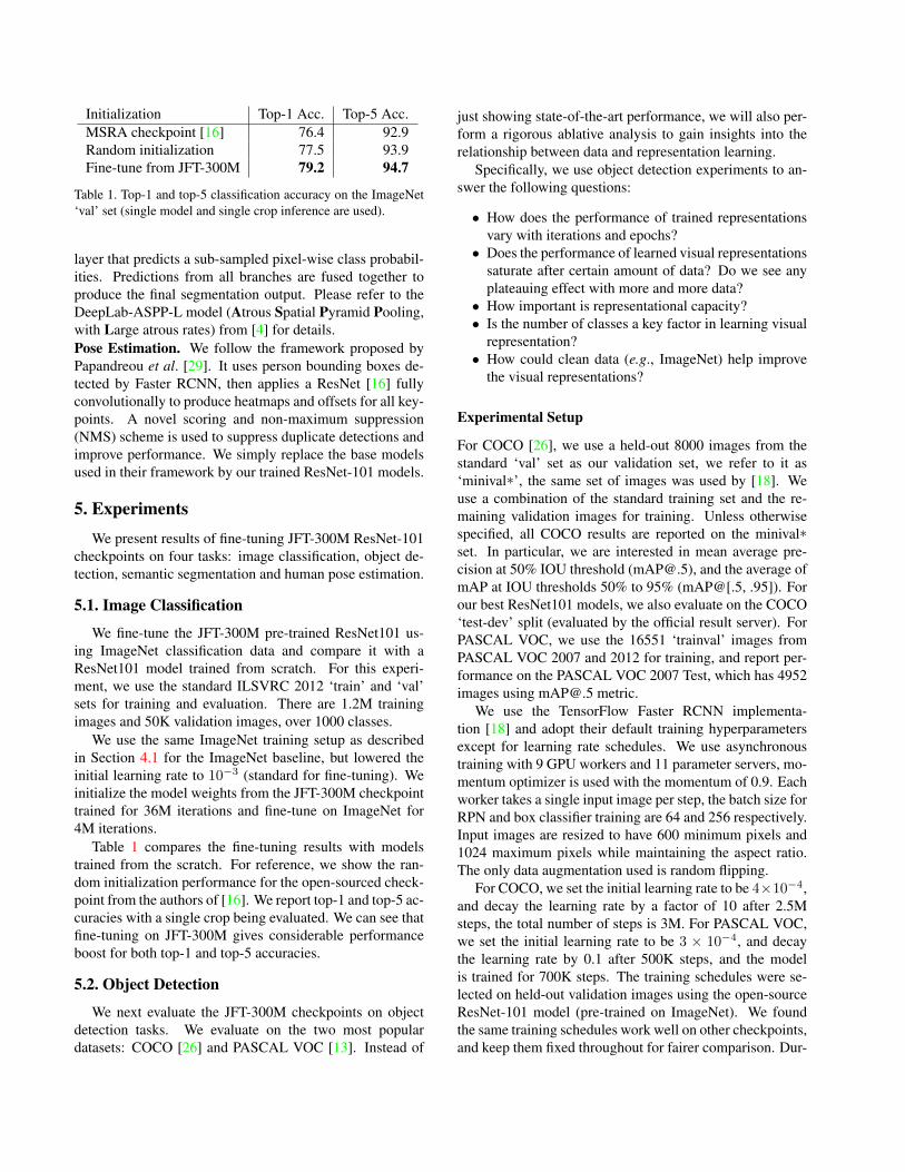
Initialization Top-1 Acc. Top-5 Acc.MSRA checkpoint [16] 76.4 92.9Random initialization 77.5 93.9Fine-tune from JFT-300M 79.2 94.7

Table 1. Top-1 and top-5 classification accuracy on the ImageNet‘val’ set (single model and single crop inference are used).

layer that predicts a sub-sampled pixel-wise class probabil-ities. Predictions from all branches are fused together toproduce the final segmentation output. Please refer to theDeepLab-ASPP-L model (Atrous Spatial Pyramid Pooling,with Large atrous rates) from [4] for details.Pose Estimation. We follow the framework proposed byPapandreou et al. [29]. It uses person bounding boxes de-tected by Faster RCNN, then applies a ResNet [16] fullyconvolutionally to produce heatmaps and offsets for all key-points. A novel scoring and non-maximum suppression(NMS) scheme is used to suppress duplicate detections andimprove performance. We simply replace the base modelsused in their framework by our trained ResNet-101 models.

5. ExperimentsWe present results of fine-tuning JFT-300M ResNet-101

checkpoints on four tasks: image classification, object de-tection, semantic segmentation and human pose estimation.

5.1. Image Classification

We fine-tune the JFT-300M pre-trained ResNet101 us-ing ImageNet classification data and compare it with aResNet101 model trained from scratch. For this experi-ment, we use the standard ILSVRC 2012 ‘train’ and ‘val’sets for training and evaluation. There are 1.2M trainingimages and 50K validation images, over 1000 classes.

We use the same ImageNet training setup as describedin Section 4.1 for the ImageNet baseline, but lowered theinitial learning rate to 10−3 (standard for fine-tuning). Weinitialize the model weights from the JFT-300M checkpointtrained for 36M iterations and fine-tune on ImageNet for4M iterations.

Table 1 compares the fine-tuning results with modelstrained from the scratch. For reference, we show the ran-dom initialization performance for the open-sourced check-point from the authors of [16]. We report top-1 and top-5 ac-curacies with a single crop being evaluated. We can see thatfine-tuning on JFT-300M gives considerable performanceboost for both top-1 and top-5 accuracies.

5.2. Object Detection

We next evaluate the JFT-300M checkpoints on objectdetection tasks. We evaluate on the two most populardatasets: COCO [26] and PASCAL VOC [13]. Instead of

just showing state-of-the-art performance, we will also per-form a rigorous ablative analysis to gain insights into therelationship between data and representation learning.

Specifically, we use object detection experiments to an-swer the following questions:

• How does the performance of trained representationsvary with iterations and epochs?• Does the performance of learned visual representations

saturate after certain amount of data? Do we see anyplateauing effect with more and more data?• How important is representational capacity?• Is the number of classes a key factor in learning visual

representation?• How could clean data (e.g., ImageNet) help improve

the visual representations?

Experimental Setup

For COCO [26], we use a held-out 8000 images from thestandard ‘val’ set as our validation set, we refer to it as‘minival∗’, the same set of images was used by [18]. Weuse a combination of the standard training set and the re-maining validation images for training. Unless otherwisespecified, all COCO results are reported on the minival∗set. In particular, we are interested in mean average pre-cision at 50% IOU threshold (mAP@.5), and the average ofmAP at IOU thresholds 50% to 95% (mAP@[.5, .95]). Forour best ResNet101 models, we also evaluate on the COCO‘test-dev’ split (evaluated by the official result server). ForPASCAL VOC, we use the 16551 ‘trainval’ images fromPASCAL VOC 2007 and 2012 for training, and report per-formance on the PASCAL VOC 2007 Test, which has 4952images using mAP@.5 metric.

We use the TensorFlow Faster RCNN implementa-tion [18] and adopt their default training hyperparametersexcept for learning rate schedules. We use asynchronoustraining with 9 GPU workers and 11 parameter servers, mo-mentum optimizer is used with the momentum of 0.9. Eachworker takes a single input image per step, the batch size forRPN and box classifier training are 64 and 256 respectively.Input images are resized to have 600 minimum pixels and1024 maximum pixels while maintaining the aspect ratio.The only data augmentation used is random flipping.

For COCO, we set the initial learning rate to be 4×10−4,and decay the learning rate by a factor of 10 after 2.5Msteps, the total number of steps is 3M. For PASCAL VOC,we set the initial learning rate to be 3 × 10−4, and decaythe learning rate by 0.1 after 500K steps, and the modelis trained for 700K steps. The training schedules were se-lected on held-out validation images using the open-sourceResNet-101 model (pre-trained on ImageNet). We foundthe same training schedules work well on other checkpoints,and keep them fixed throughout for fairer comparison. Dur-

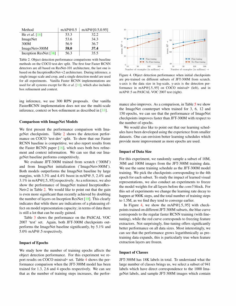
Method mAP@0.5 mAP@[0.5,0.95]He et al. [16] 53.3 32.2ImageNet 53.6 34.3300M 56.9 36.7ImageNet+300M 58.0 37.4Inception ResNet [38] 56.3 35.5

Table 2. Object detection performance comparisons with baselinemethods on the COCO test-dev split. The first four Faster RCNNdetectors are all based on ResNet-101 architecture, the last one isbased on the InceptionResNet-v2 architecture. During inference, asingle image scale and crop, and a single detection model are usedfor all experiments. Vanilla Faster RCNN implementations areused for all systems except for He et al. [16], which also includesbox refinement and context.

ing inference, we use 300 RPN proposals. Our vanillaFasterRCNN implementation does not use the multi-scaleinference, context or box-refinement as described in [33].

Comparison with ImageNet Models

We first present the performance comparison with Ima-geNet checkpoints. Table 2 shows the detection perfor-mance on COCO ‘test-dev’ split. To show that our FasterRCNN baseline is competitive, we also report results fromthe Faster RCNN paper [16], which uses both box refine-ment and context information. We can see that our Ima-geNet baseline performs competitively.

We evaluate JFT-300M trained from scratch (‘300M’)and from ImageNet initialization (’ImageNet+300M’).Both models outperforms the ImageNet baseline by largemargins, with 3.3% and 4.4% boost in mAP@.5, 2.4% and3.1% in mAP@[.5,.95] respectively. As a reference, we alsoshow the performance of ImageNet trained InceptionRes-Netv2 in Table 2. We would like to point out that the gainis even more significant than recently achieved by doublingthe number of layers on Inception ResNet [18]. This clearlyindicates that while there are indications of a plateauing ef-fect on model representation capacity; in terms of data thereis still a lot that can be easily gained.

Table 3 shows the performance on the PASCAL VOC2007 ‘test’ set. Again, both JFT-300M checkpoints out-performs the ImageNet baseline significantly, by 5.1% and5.0% mAP@.5 respectively.

Impact of Epochs

We study how the number of training epochs affects theobject detection performance. For this experiment we re-port results on COCO minival∗ set. Table 4 shows the per-formance comparison when the JFT-300M model has beentrained for 1.3, 2.6 and 4 epochs respectively. We can seethat as the number of training steps increases, the perfor-

10 30 100 300

Number of examples (in millions) →0

10

20

30

40

mea

nA

P→

Fine-tuning

No Fine-tuning

10 30 100 300

Number of examples (in millions) →

40

60

80

mea

nA

P→

Fine-tuning

No Fine-tuning

Figure 4. Object detection performance when initial checkpointsare pre-trained on different subsets of JFT-300M from scratch.x-axis is the data size in log-scale, y-axis is the detection per-formance in mAP@[.5,.95] on COCO minival∗ (left), and inmAP@.5 on PASCAL VOC 2007 test (right).

mance also improves. As a comparison, in Table 5 we showthe ImageNet counterpart when trained for 3, 6, 12 and150 epochs, we can see that the performance of ImageNetcheckpoints improves faster than JFT-300M with respect tothe number of epochs.

We would also like to point out that our learning sched-ules have been developed using the experience from smallerdatasets. One can envision better learning schedules whichprovide more improvement as more epochs are used.

Impact of Data Size

For this experiment, we randomly sample a subset of 10M,30M and 100M images from the JFT-300M training data.We use the same training schedule as the JFT-300M modeltraining. We pick the checkpoints corresponding to the 4thepoch for each subset. To study the impact of learned visualrepresentations, we also conduct an experiments to freezethe model weights for all layers before the conv5 block. Forthis set of experiments we change the learning rate decay tohappen at 900K steps, and the total number of training stepsto 1.5M, as we find they tend to converge earlier.

In Figure 4, we show the mAP@[.5,.95] with check-points trained on different JFT-300M subsets, the blue curvecorresponds to the regular faster RCNN training (with fine-tuning), while the red curve corresponds to freezing featureextractors. Not surprisingly, fine-tuning offers significantlybetter performance on all data sizes. Most interestingly, wecan see that the performance grows logarithmically as pre-training data expands, this is particularly true when featureextraction layers are frozen.

Impact of Classes

JFT-300M has 18K labels in total. To understand what thelarge number of classes brings us, we select a subset of 941labels which have direct correspondence to the 1000 Ima-geNet labels, and sample JFT-300M images which contain

method airplane bicycle bird boat bottle bus car cat chair cow table dog horse mbike person plant sheep sofa train TV meanImageNet 79.7 80.6 77.1 65.9 64.2 85.3 81.0 88.4 60.5 83.1 70.8 86.7 86.2 79.7 79.5 49.5 78.3 80.2 79.2 69.7 76.3300M 87.2 88.8 79.6 75.2 67.9 88.2 89.3 88.6 64.3 86.1 73.6 88.7 89.1 86.5 86.4 57.7 84.2 82.1 86.7 78.6 81.4ImageNet+300M 86.9 88.0 80.1 74.7 68.8 88.9 89.6 88.0 69.7 86.9 71.9 88.5 89.6 86.9 86.8 53.7 78.2 82.3 87.7 77.9 81.3

Table 3. Average Precision @ IOU threshold of 0.5 on PASCAL VOC 2007 ‘test’ set. The ‘trainval’ set of PASCAL VOC 2007 and 2012are used for training.

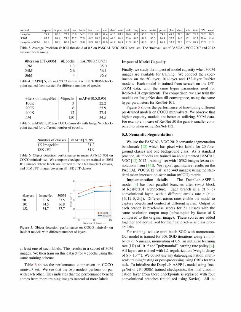
#Iters on JFT-300M #Epochs mAP@[0.5,0.95]12M 1.3 35.024M 2.6 36.136M 4 36.8

Table 4. mAP@[.5,.95] on COCO minival∗ with JFT-300M check-point trained from scratch for different number of epochs.

#Iters on ImageNet #Epochs mAP@[0.5,0.95]100K 3 22.2200K 6 25.9400K 12 27.45M 150 34.5

Table 5. mAP@[.5,.95] on COCO minival∗ with ImageNet check-point trained for different number of epochs.

Number of classes mAP@[.5,.95]1K ImageNet 31.218K JFT 31.9

Table 6. Object detection performance in mean AP@[.5,.95] onCOCO minival∗ set. We compare checkpoints pre-trained on 30MJFT images where labels are limited to the 1K ImageNet classes,and 30M JFT images covering all 18K JFT classes.

#Layers ImageNet 300M50 31.6 33.5101 34.5 36.8152 34.7 37.7

50 101 152

Number of layers →20

25

30

35

40

mea

nA

P→

300M

ImageNet

Figure 5. Object detection performance on COCO minival∗ onResNet models with different number of layers.

at least one of such labels. This results in a subset of 30Mimages. We then train on this dataset for 4 epochs using thesame training scheme.

Table 6 shows the performance comparison on COCOminival∗ set. We see that the two models perform on parwith each other. This indicates that the performance benefitcomes from more training images instead of more labels.

Impact of Model Capacity

Finally, we study the impact of model capacity when 300Mimages are available for training. We conduct the exper-iments on the 50-layer, 101-layer and 152-layer ResNetmodels. Each model is trained from scratch on the JFT-300M data, with the same hyper parameters used forResNet-101 experiments. For comparison, we also train themodels on ImageNet data till convergence, using the samehyper parameters for ResNet-101.

Figure 5 shows the performance of fine-tuning differentpre-trained models on COCO minival∗set. We observe thathigher capacity models are better at utilizing 300M data.For example, in case of ResNet-50 the gain is smaller com-pared to when using ResNet-152.

5.3. Semantic Segmentation

We use the PASCAL VOC 2012 semantic segmentationbenchmark [12] which has pixel-wise labels for 20 fore-ground classes and one background class. As is standardpractice, all models are trained on an augmented PASCALVOC [12] 2012 ‘trainaug’ set with 10582 images (extra an-notations from [15]). We report quantitative results on thePASCAL VOC 2012 ‘val’ set (1449 images) using the stan-dard mean intersection-over-union (mIOU) metric.

Implementation details. The DeepLab-ASPP-Lmodel [4] has four parallel branches after conv5 blockof ResNet101 architecture. Each branch is a (3 × 3)convolutional layer, with a different atrous rate r (r ∈{6, 12, 8, 24}). Different atrous rates enable the model tocapture objects and context at different scales. Output ofeach branch is pixel-wise scores for 21 classes with thesame resolution output map (subsampled by factor of 8compared to the original image). These scores are addedtogether and normalized for the final pixel-wise class prob-abilities.

For training, we use mini-batch SGD with momentum.Our model is trained for 30k SGD iterations using a mini-batch of 6 images, momentum of 0.9, an initialize learningrate (LR) of 10−3 and ”polynomial” learning rate policy [4].All layers are trained with L2-regularization (weight decayof 5× 10−4). We do not use any data-augmentation, multi-scale training/testing or post-processing using CRFs for thistask. To initialize the DeepLab-ASPP-L model using Ima-geNet or JFT-300M trained checkpoints, the final classifi-cation layer from these checkpoints is replaced with fourconvolutional branches (initialized using Xavier). All in-

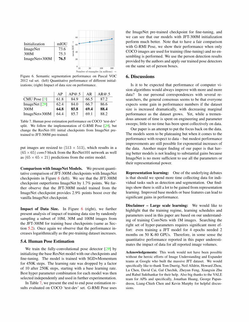
Initialization mIOUImageNet 73.6300M 75.3ImageNet+300M 76.5

10 30 100 300

Number of examples (in millions) →

0

20

40

60

80

mea

nIO

U →

Figure 6. Semantic segmentation performance on Pascal VOC2012 val set. (left) Quantitative performance of different initial-izations; (right) Impact of data size on performance.

AP AP@.5 AR AR@.5CMU Pose [3] 61.8 84.9 66.5 87.2ImageNet [29] 62.4 84.0 66.7 86.6300M 64.8 85.8 69.4 88.4ImageNet+300M 64.4 85.7 69.1 88.2

Table 7. Human pose estimation performance on COCO ‘test-dev’split. We follow the implementation of G-RMI Pose [29], butchange the ResNet-101 initial checkpoints from ImageNet pre-trained to JFT-300M pre-trained.

put images are resized to (513 × 513), which results in a(65× 65) conv5 block from the ResNet101 network as wellas (65× 65× 21) predictions from the entire model.

Comparison with ImageNet Models. We present quanti-tative comparison of JFT-300M checkpoints with ImageNetcheckpoints in Figure 6 (left). We see that the JFT-300Mcheckpoint outperforms ImageNet by 1.7% points. We fur-ther observe that the JFT-300M model trained from theImageNet checkpoint provides 2.9% points boost over thevanilla ImageNet checkpoint.

Impact of Data Size. In Figure 6 (right), we furtherpresent analysis of impact of training data size by randomlysampling a subset of 10M, 30M and 100M images fromthe JFT-300M for training base checkpoints (same as Sec-tion 5.2). Once again we observe that the performance in-creases logarithmically as the pre-training dataset increases.

5.4. Human Pose Estimation

We train the fully-convolutional pose detector [29] byinitializing the base ResNet model with our checkpoints andfine-tuning. The model is trained with SGD+Momentumfor 450K steps. The learning rate was dropped by a factorof 10 after 250K steps, starting with a base learning rate.Best hyper parameter combination for each model was thenselected independently and used in further experimentation.

In Table 7, we present the end to end pose estimation re-sults evaluated on COCO ‘test-dev’ set. G-RMI Pose uses

the ImageNet pre-trained checkpoint for fine-tuning, andwe can see that our models with JFT-300M initializationperform much better. Note that to have a fair comparisonwith G-RMI Pose, we show their performance when onlyCOCO images are used for training (fine-tuning) and no en-sembling is performed. We use the person detection resultsprovided by the authors and apply our trained pose detectorson the same set of person boxes.

6. Discussions

Is it to be expected that performance of computer vi-sion algorithms would always improve with more and moredata? In our personal correspondences with several re-searchers, the general consensus seems to be that everyoneexpects some gain in performance numbers if the datasetsize is increased dramatically, with decreasing marginalperformance as the dataset grows. Yet, while a tremen-dous amount of time is spent on engineering and parametersweeps; little to no time has been spent collectively on data.

Our paper is an attempt to put the focus back on the data.The models seem to be plateauing but when it comes to theperformance with respect to data – but modest performanceimprovements are still possible for exponential increases ofthe data. Another major finding of our paper is that hav-ing better models is not leading to substantial gains becauseImageNet is no more sufficient to use all the parameters ortheir representational power.

Representation learning: One of the underlying debatesis that should we spend more time collecting data for indi-vidual tasks such as detection and segmentation. Our find-ings show there is still a lot to be gained from representationlearning. Improved base models or base features can lead tosignificant gains in performance.

Disclaimer – Large scale learning: We would like tohighlight that the training regime, learning schedules andparameters used in this paper are based on our understand-ing of training ConvNets with 1M images. Searching theright set of hyper-parameters requires significant more ef-fort: even training a JFT model for 4 epochs needed 2months on 50 K-80 GPUs. Therefore, in some sense thequantitative performance reported in this paper underesti-mates the impact of data for all reported image volumes.

Acknowledgements: This work would not have been possiblewithout the heroic efforts of Image Understanding and Expanderteams at Google who built the massive JFT dataset. We wouldspecifically like to thank Tom Duerig, Neil Alldrin, Howard Zhou,Lu Chen, David Cai, Gal Chechik, Zheyun Feng, Xiangxin Zhuand Rahul Sukthankar for their help. Also big thanks to the VALEteam for APIs and specifically, Jonathan Huang, George Papan-dreou, Liang-Chieh Chen and Kevin Murphy for helpful discus-sions.

References[1] P. Agrawal, R. B. Girshick, and J. Malik. Analyzing the per-

formance of multilayer neural networks for object recogni-tion. In ECCV, 2014.

[2] A. Bergamo and L. Torresani. Exploiting weakly-labeledweb images to improve object classification: a domain adap-tation approach. In NIPS. 2010.

[3] Z. Cao, T. Simon, S. Wei, and Y. Sheikh. Realtimemulti-person 2d pose estimation using part affinity fields.arXiv:1611.08050, 2016.

[4] L.-C. Chen, G. Papandreou, I. Kokkinos, K. Murphy, andA. L. Yuille. Deeplab: Semantic image segmentation withdeep convolutional nets, atrous convolution, and fully con-nected crfs. arXiv preprint arXiv:1606.00915, 2016.

[5] X. Chen and A. Gupta. Webly supervised learning of convo-lutional networks. In ICCV, 2015.

[6] X. Chen, A. Shrivastava, and A. Gupta. Neil: Extractingvisual knowledge from web data. In ICCV, 2013.

[7] F. Chollet. Xception: Deep learning with depthwise separa-ble convolutions. arXiv:1610.02357, 2016.

[8] J. Dean, G. Corrado, R. Monga, K. Chen, M. Devin, Q. V. Le,M. Z. Mao, M. Ranzato, A. W. Senior, P. A. Tucker, K. Yang,and A. Y. Ng. Large scale distributed deep networks. InNIPS, 2012.

[9] S. Divvala, A. Farhadi, and C. Guestrin. Learning everythingabout anything: Webly-supervised visual concept learning.In CVPR, 2014.

[10] C. Doersch, A. Gupta, and A. A. Efros. Unsupervised vi-sual representation learning by context prediction. In ICCV,2015.

[11] J. Donahue, P. Krahenbuhl, and T. Darrell. Adversarial fea-ture learning. arXiv:1605.09782, 2016.

[12] M. Everingham, L. Van Gool, C. K. Williams, J. Winn, andA. Zisserman. The Pascal Visual Object Classes (VOC)Challenge. IJCV, 2010.

[13] M. Everingham, L. Van Gool, C. K. I. Williams, J. Winn,and A. Zisserman. The pascal visual object classes (voc)challenge. IJCV, 2010.

[14] R. B. Girshick, J. Donahue, T. Darrell, and J. Malik. Richfeature hierarchies for accurate object detection and semanticsegmentation. arXiv:1311.2524, 2013.

[15] B. Hariharan, P. Arbelaez, L. Bourdev, S. Maji, and J. Malik.Semantic contours from inverse detectors. In ICCV, 2011.

[16] K. He, X. Zhang, S. Ren, and J. Sun. Deep residual learningfor image recognition. In CVPR, 2016.

[17] G. Hinton, O. Vinyals, and J. Dean. Distilling the knowledgein a neural network. In NIPS, 2014.

[18] J. Huang, V. Rathod, C. Sun, M. Zhu, A. Korattikara,A. Fathi, I. Fischer, Z. Wojna, Y. Song, S. Guadarrama, andK. Murphy. Speed/accuracy trade-offs for modern convolu-tional object detectors. In CVPR, 2017.

[19] M. Huh, P. Agrawal, and A. A. Efros. What makes imagenetgood for transfer learning? arXiv:1608.08614, 2016.

[20] S. Ioffe and C. Szegedy. Batch normalization: Acceleratingdeep network training by reducing internal covariate shift.arXiv:1502.03167, 2015.

[21] H. Izadinia, B. C. Russell, A. Farhadi, M. D. Hoffman, andA. Hertzmann. Deep classifiers from image tags in the wild.In ACM MM, 2015.

[22] M. Jain, J. C. van Gemert, and C. G. Snoek. What do 15,000object categories tell us about classifying and localizing ac-tions? In CVPR, 2015.

[23] A. Joulin, L. van der Maaten, A. Jabri, and N. Vasilache.Learning visual features from large weakly supervised data.arXiv:1511.02251, 2015.

[24] J. Krause, B. Sapp, A. Howard, H. Zhou, A. Toshev,T. Duerig, J. Philbin, and F. Li. The unreasonableeffectiveness of noisy data for fine-grained recognition.arXiv:1511.06789, 2015.

[25] A. Krizhevsky, I. Sutskever, and G. E. Hinton. Imagenetclassification with deep convolutional neural networks. InNIPS, 2012.

[26] T. Lin, M. Maire, S. J. Belongie, J. Hays, P. Perona, D. Ra-manan, P. Dollar, and C. L. Zitnick. Microsoft COCO: com-mon objects in context. In ECCV, 2014.

[27] K. Ni, R. A. Pearce, K. Boakye, B. V. Essen, D. Borth,B. Chen, and E. X. Wang. Large-scale deep learning on theYFCC100M dataset. arXiv:1502.03409, 2015.

[28] M. Oquab, L. Bottou, I. Laptev, and J. Sivic. Learning andtransferring mid-level image representations using convolu-tional neural networks. In CVPR, 2014.

[29] G. Papandreou, T. Zhu, N. Kanazawa, A. Toshev, J. Tomp-son, C. Bregler, and K. Murphy. Towards accurate multi-person pose estimation in the wild. arXiv:1701.01779, 2017.

[30] F. Pereira, P. Norvig, and A. Halev. The unreasonable effec-tiveness of data. IEEE Intelligent Systems, 2009.

[31] L. Pinto, D. Gandhi, Y. Han, Y. Park, and A. Gupta. Thecurious robot: Learning visual representations via physicalinteractions. arXiv:1604.01360, 2016.

[32] L. Pinto and A. Gupta. Supersizing self-supervision:Learning to grasp from 50k tries and 700 robot hours.arXiv:1509.06825, 2015.

[33] S. Ren, K. He, R. Girshick, and J. Sun. Faster R-CNN: To-wards real-time object detection with region proposal net-works. In NIPS, 2015.

[34] M. Rubinstein, A. Joulin, J. Kopf, and C. Liu. Unsupervisedjoint object discovery and segmentation in internet images.CVPR, 2013.

[35] O. Russakovsky, J. Deng, H. Su, J. Krause, S. Satheesh,S. Ma, Z. Huang, A. Karpathy, A. Khosla, M. S. Bernstein,A. C. Berg, and F. Li. Imagenet large scale visual recognitionchallenge. arXiv:1409.0575, 2014.

[36] K. Simonyan and A. Zisserman. Two-stream convolutionalnetworks for action recognition in videos. arXiv:1406.2199,2014.

[37] K. Simonyan and A. Zisserman. Very deep con-volutional networks for large-scale image recognition.arXiv:1409.1556, 2014.

[38] C. Szegedy, S. Ioffe, and V. Vanhoucke. Inception-v4,inception-resnet and the impact of residual connections onlearning. arXiv:1602.07261, 2016.

[39] C. Szegedy, W. Liu, Y. Jia, P. Sermanet, S. Reed,D. Anguelov, D. Erhan, V. Vanhoucke, and A. Rabinovich.Going deeper with convolutions. In CVPR, 2015.

[40] B. Thomee, D. A. Shamma, G. Friedland, B. Elizalde, K. Ni,D. Poland, D. Borth, and L. Li. The new data and new chal-lenges in multimedia research. arXiv:1503.01817, 2015.

[41] A. Torralba and A. Efros. Unbiased look at dataset bias.CVPR, 2011.

[42] C. Vondrick, H. Pirsiavash, and A. Torralba. Generatingvideos with scene dynamics. In NIPS, 2016.

[43] X. Wang and A. Gupta. Unsupervised learning of visual rep-resentations using videos. arXiv:1505.00687, 2015.

[44] T. Weyand, I. Kostrikov, and J. Philbin. Planet -photo geolocation with convolutional neural networks.arXiv:1602.05314, 2016.

Appendix ADe-duplication Experiments

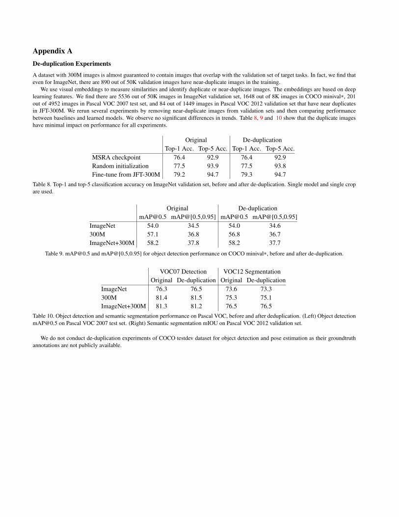
A dataset with 300M images is almost guaranteed to contain images that overlap with the validation set of target tasks. In fact, we find thateven for ImageNet, there are 890 out of 50K validation images have near-duplicate images in the training.

We use visual embeddings to measure similarities and identify duplicate or near-duplicate images. The embeddings are based on deeplearning features. We find there are 5536 out of 50K images in ImageNet validation set, 1648 out of 8K images in COCO minival∗, 201out of 4952 images in Pascal VOC 2007 test set, and 84 out of 1449 images in Pascal VOC 2012 validation set that have near duplicatesin JFT-300M. We rerun several experiments by removing near-duplicate images from validation sets and then comparing performancebetween baselines and learned models. We observe no significant differences in trends. Table 8, 9 and 10 show that the duplicate imageshave minimal impact on performance for all experiments.

Original De-duplicationTop-1 Acc. Top-5 Acc. Top-1 Acc. Top-5 Acc.

MSRA checkpoint 76.4 92.9 76.4 92.9Random initialization 77.5 93.9 77.5 93.8Fine-tune from JFT-300M 79.2 94.7 79.3 94.7

Table 8. Top-1 and top-5 classification accuracy on ImageNet validation set, before and after de-duplication. Single model and single cropare used.

Original De-duplicationmAP@0.5 mAP@[0.5,0.95] mAP@0.5 mAP@[0.5,0.95]

ImageNet 54.0 34.5 54.0 34.6300M 57.1 36.8 56.8 36.7ImageNet+300M 58.2 37.8 58.2 37.7

Table 9. mAP@0.5 and mAP@[0.5,0.95] for object detection performance on COCO minival∗, before and after de-duplication.

VOC07 Detection VOC12 SegmentationOriginal De-duplication Original De-duplication

ImageNet 76.3 76.5 73.6 73.3300M 81.4 81.5 75.3 75.1ImageNet+300M 81.3 81.2 76.5 76.5

Table 10. Object detection and semantic segmentation performance on Pascal VOC, before and after deduplication. (Left) Object detectionmAP@0.5 on Pascal VOC 2007 test set. (Right) Semantic segmentation mIOU on Pascal VOC 2012 validation set.

We do not conduct de-duplication experiments of COCO testdev dataset for object detection and pose estimation as their groundtruthannotations are not publicly available.

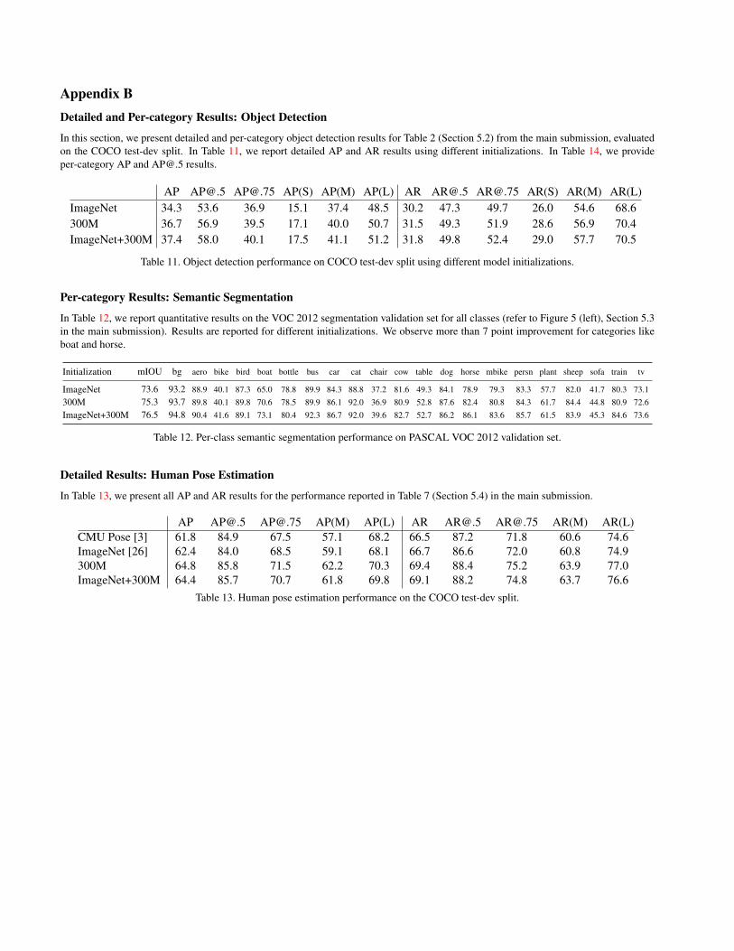
Appendix BDetailed and Per-category Results: Object Detection

In this section, we present detailed and per-category object detection results for Table 2 (Section 5.2) from the main submission, evaluatedon the COCO test-dev split. In Table 11, we report detailed AP and AR results using different initializations. In Table 14, we provideper-category AP and AP@.5 results.

AP AP@.5 AP@.75 AP(S) AP(M) AP(L) AR AR@.5 AR@.75 AR(S) AR(M) AR(L)ImageNet 34.3 53.6 36.9 15.1 37.4 48.5 30.2 47.3 49.7 26.0 54.6 68.6300M 36.7 56.9 39.5 17.1 40.0 50.7 31.5 49.3 51.9 28.6 56.9 70.4ImageNet+300M 37.4 58.0 40.1 17.5 41.1 51.2 31.8 49.8 52.4 29.0 57.7 70.5

Table 11. Object detection performance on COCO test-dev split using different model initializations.

Per-category Results: Semantic Segmentation

In Table 12, we report quantitative results on the VOC 2012 segmentation validation set for all classes (refer to Figure 5 (left), Section 5.3in the main submission). Results are reported for different initializations. We observe more than 7 point improvement for categories likeboat and horse.

Initialization mIOU bg aero bike bird boat bottle bus car cat chair cow table dog horse mbike persn plant sheep sofa train tv

ImageNet 73.6 93.2 88.9 40.1 87.3 65.0 78.8 89.9 84.3 88.8 37.2 81.6 49.3 84.1 78.9 79.3 83.3 57.7 82.0 41.7 80.3 73.1300M 75.3 93.7 89.8 40.1 89.8 70.6 78.5 89.9 86.1 92.0 36.9 80.9 52.8 87.6 82.4 80.8 84.3 61.7 84.4 44.8 80.9 72.6ImageNet+300M 76.5 94.8 90.4 41.6 89.1 73.1 80.4 92.3 86.7 92.0 39.6 82.7 52.7 86.2 86.1 83.6 85.7 61.5 83.9 45.3 84.6 73.6

Table 12. Per-class semantic segmentation performance on PASCAL VOC 2012 validation set.

Detailed Results: Human Pose Estimation

In Table 13, we present all AP and AR results for the performance reported in Table 7 (Section 5.4) in the main submission.

AP AP@.5 AP@.75 AP(M) AP(L) AR AR@.5 AR@.75 AR(M) AR(L)CMU Pose [3] 61.8 84.9 67.5 57.1 68.2 66.5 87.2 71.8 60.6 74.6ImageNet [26] 62.4 84.0 68.5 59.1 68.1 66.7 86.6 72.0 60.8 74.9300M 64.8 85.8 71.5 62.2 70.3 69.4 88.4 75.2 63.9 77.0ImageNet+300M 64.4 85.7 70.7 61.8 69.8 69.1 88.2 74.8 63.7 76.6

Table 13. Human pose estimation performance on the COCO test-dev split.

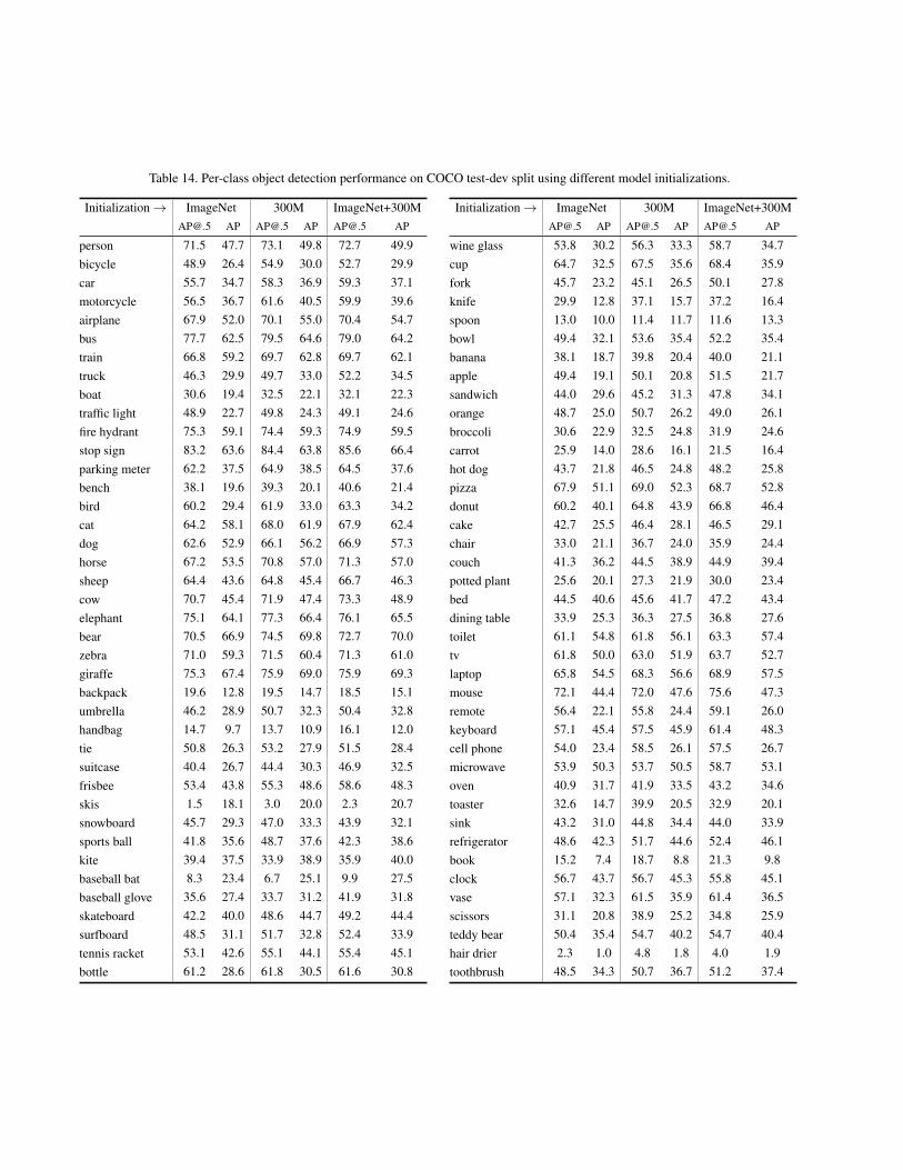
Table 14. Per-class object detection performance on COCO test-dev split using different model initializations.

Initialization → ImageNet 300M ImageNet+300MAP@.5 AP AP@.5 AP AP@.5 AP

person 71.5 47.7 73.1 49.8 72.7 49.9bicycle 48.9 26.4 54.9 30.0 52.7 29.9car 55.7 34.7 58.3 36.9 59.3 37.1motorcycle 56.5 36.7 61.6 40.5 59.9 39.6airplane 67.9 52.0 70.1 55.0 70.4 54.7bus 77.7 62.5 79.5 64.6 79.0 64.2train 66.8 59.2 69.7 62.8 69.7 62.1truck 46.3 29.9 49.7 33.0 52.2 34.5boat 30.6 19.4 32.5 22.1 32.1 22.3traffic light 48.9 22.7 49.8 24.3 49.1 24.6fire hydrant 75.3 59.1 74.4 59.3 74.9 59.5stop sign 83.2 63.6 84.4 63.8 85.6 66.4parking meter 62.2 37.5 64.9 38.5 64.5 37.6bench 38.1 19.6 39.3 20.1 40.6 21.4bird 60.2 29.4 61.9 33.0 63.3 34.2cat 64.2 58.1 68.0 61.9 67.9 62.4dog 62.6 52.9 66.1 56.2 66.9 57.3horse 67.2 53.5 70.8 57.0 71.3 57.0sheep 64.4 43.6 64.8 45.4 66.7 46.3cow 70.7 45.4 71.9 47.4 73.3 48.9elephant 75.1 64.1 77.3 66.4 76.1 65.5bear 70.5 66.9 74.5 69.8 72.7 70.0zebra 71.0 59.3 71.5 60.4 71.3 61.0giraffe 75.3 67.4 75.9 69.0 75.9 69.3backpack 19.6 12.8 19.5 14.7 18.5 15.1umbrella 46.2 28.9 50.7 32.3 50.4 32.8handbag 14.7 9.7 13.7 10.9 16.1 12.0tie 50.8 26.3 53.2 27.9 51.5 28.4suitcase 40.4 26.7 44.4 30.3 46.9 32.5frisbee 53.4 43.8 55.3 48.6 58.6 48.3skis 1.5 18.1 3.0 20.0 2.3 20.7snowboard 45.7 29.3 47.0 33.3 43.9 32.1sports ball 41.8 35.6 48.7 37.6 42.3 38.6kite 39.4 37.5 33.9 38.9 35.9 40.0baseball bat 8.3 23.4 6.7 25.1 9.9 27.5baseball glove 35.6 27.4 33.7 31.2 41.9 31.8skateboard 42.2 40.0 48.6 44.7 49.2 44.4surfboard 48.5 31.1 51.7 32.8 52.4 33.9tennis racket 53.1 42.6 55.1 44.1 55.4 45.1bottle 61.2 28.6 61.8 30.5 61.6 30.8

Initialization → ImageNet 300M ImageNet+300MAP@.5 AP AP@.5 AP AP@.5 AP

wine glass 53.8 30.2 56.3 33.3 58.7 34.7cup 64.7 32.5 67.5 35.6 68.4 35.9fork 45.7 23.2 45.1 26.5 50.1 27.8knife 29.9 12.8 37.1 15.7 37.2 16.4spoon 13.0 10.0 11.4 11.7 11.6 13.3bowl 49.4 32.1 53.6 35.4 52.2 35.4banana 38.1 18.7 39.8 20.4 40.0 21.1apple 49.4 19.1 50.1 20.8 51.5 21.7sandwich 44.0 29.6 45.2 31.3 47.8 34.1orange 48.7 25.0 50.7 26.2 49.0 26.1broccoli 30.6 22.9 32.5 24.8 31.9 24.6carrot 25.9 14.0 28.6 16.1 21.5 16.4hot dog 43.7 21.8 46.5 24.8 48.2 25.8pizza 67.9 51.1 69.0 52.3 68.7 52.8donut 60.2 40.1 64.8 43.9 66.8 46.4cake 42.7 25.5 46.4 28.1 46.5 29.1chair 33.0 21.1 36.7 24.0 35.9 24.4couch 41.3 36.2 44.5 38.9 44.9 39.4potted plant 25.6 20.1 27.3 21.9 30.0 23.4bed 44.5 40.6 45.6 41.7 47.2 43.4dining table 33.9 25.3 36.3 27.5 36.8 27.6toilet 61.1 54.8 61.8 56.1 63.3 57.4tv 61.8 50.0 63.0 51.9 63.7 52.7laptop 65.8 54.5 68.3 56.6 68.9 57.5mouse 72.1 44.4 72.0 47.6 75.6 47.3remote 56.4 22.1 55.8 24.4 59.1 26.0keyboard 57.1 45.4 57.5 45.9 61.4 48.3cell phone 54.0 23.4 58.5 26.1 57.5 26.7microwave 53.9 50.3 53.7 50.5 58.7 53.1oven 40.9 31.7 41.9 33.5 43.2 34.6toaster 32.6 14.7 39.9 20.5 32.9 20.1sink 43.2 31.0 44.8 34.4 44.0 33.9refrigerator 48.6 42.3 51.7 44.6 52.4 46.1book 15.2 7.4 18.7 8.8 21.3 9.8clock 56.7 43.7 56.7 45.3 55.8 45.1vase 57.1 32.3 61.5 35.9 61.4 36.5scissors 31.1 20.8 38.9 25.2 34.8 25.9teddy bear 50.4 35.4 54.7 40.2 54.7 40.4hair drier 2.3 1.0 4.8 1.8 4.0 1.9toothbrush 48.5 34.3 50.7 36.7 51.2 37.4