Revolutionary Physics-Based Design Tools for Quiet …personal.psu.edu/lnl/papers/AIAA-2006-1068.pdf · Revolutionary Physics-Based ... L.N. Sankar2, S. Menon3, O ... These aspects

Revolutionary Physics-Based Design Tools for Quiet Helicopters

E.P.N. Duque 1 Northern Arizona University, Flagstaff, AZ, 86011, United States

L.N. Sankar2, S. Menon3, O. Bauchau4, S. Ruffin5, M. Smith6, K. Ahuja7

Georgia Institute of Technology, Atlanta, GA, 30332-0150

K.S. Brentner8, L.N. Long9, P.J. Morris10, F. Gandhi11

Pennsylvania State University, University Park, PA 16802

This paper describes a revolutionary, fully-integrated approach for modeling the noisecharacteristics of maneuvering rotorcraft. The primary objective of this effort is the devel-opment of a physics-based software tool that enables the design of quiet rotors without per-formance penalties. This tool shall accurately predict the rotorcraft flight state and rotortrim, the unsteady aerodynamic loading, the time-dependent flow field around the rotorblades, and the radiated noise, in all flight conditions including maneuver. This objective isachieved through the use of advanced computational fluid dynamics (CFD), computationalstructural dynamics (CSD), and computational aeroacoustics (CAA). The predictions arevalidated and verified against benchmark test cases. The advanced CFD methods include in-novations in Large Eddy Simulation, novel techniques for flexible deforming blades, high-or-der methods for accuracy, and adaptive grids to accurately capture important flow features.CSD methods are coupled with the CFD and acoustics codes using generic interfaces. Theaeroacoustic predictions build on an advanced method with enhancements for maneuveringflight.

I.Introductionccurate prediction of the noise characteristics of contemporary and next-generation helicopters requires a de-tailed knowledge of the aerodynamic flow field around the rotor blades. Aerodynamic and aeroacoustic model-

ing both require an accurate description of the blade position and motion, which in turn requires an accurate model-ing of the aeroelastic response of the blade surfaces in conjunction with the control setting imposed by the pilot totrim the vehicle. For most vehicles, the trim conditions will vary with time, particularly during aggressive maneu-vers. These aspects ultimately affect the noise characteristics of the helicopter and are tightly coupled to each other.

A

The DARPA Helicopter Quieting Program focuses on the revolutionary design of rotor blades that will dramati-cally reduce the rotor noise without sacrificing flight performance. However, attempts to predict rotorcraft aeroa-coustics have had difficulties because it was not possible to fully and consistently account for the tight coupling be-tween the aircraft aerodynamics, aeroacoustics, aeroelasticity, and aircraft trim. Furthermore, the lack of adequatephysics-based design and analysis tools limited the ability of rotorcraft designers to design next generation low noiserotorcraft. The request from DARPA for computational tools capable of addressing the design of new low-noise ro-torcraft designs has led to the work summarized in this paper.

1 Associate Professor, Department of Mechanical Engineering, Senior Member AIAA.

2 Regents Professor and Associate Chair , School of Aerospace Engineering, Associate Fellow AIAA.

3 Professor, School of Aerospace Engineering, Associate Fellow AIAA.

4 Professor, School of Aerospace Engineering, AIAA Senior Member.

5 Associate Professor, School of Aerospace Engineering, AIAA Senior Member.

6 Associate Professor, School of Aerospace Engineering, Associate Fellow AIAA.

7 Regents Researcher and Professor of Aerospace Engineering, School of Aerospace Engineering, Fellow AIAA.

8 Associate Professor, Department of Aerospace Engineering, Associate Fellow AIAA.

9 Professor, Department of Aerospace Engineering, Fellow AIAA.

10 Boeing/A. D. Welliver Professor of Aerospace Engineering (and Acoustics), Department of Aerospace Engineering, Fellow AIAA.

11 Associate Professor, Department of Aerospace Engineering, Senior Member AIAA.

1American Institute of Aeronautics and Astronautics

Lyle

AIAA Paper No. 2006-1068

Integration Surface

Key to this effort is the use of Large Eddy Simulation (LES) methods in predicting the aerodynamic loads on thethe rotor. Rotary wing flight consists of various flow states along the rotor disks. On the advancing side the rotormay experience transonic flow causing shocks to form. On the retreating side, the rotor blade experiences high an-gles of attack and reversed flow. At extreme operating conditions, shock induced separation may occur on the ad-vancing side while dynamic stall events and massive stall may occur on the retreating. Accounting for these eventsand the need to obtain accurate rotor trim states is key to properly capturing the rotor noise.

The major challenge here is to develop a computational tool capable of capturing the noise of a rotorcraft, whichcan be classified as: (1) thickness and loading noise (together known as rotational noise); (2) blade-vortex-interac-tion (BVI) noise, a type of loading noise caused by impulsive loading; (3) broadband noise, a type of loading noisedue to several stochastic loading mechanisms; (4) high-speed impulsive (HSI) noise, which is associated with tran-sonic flow and shocks on the advancing rotor; and (5) transient maneuver noise, which is an additional source ofthickness and loading noise that occurs during short-duration, rapid maneuvers—typical of military operations.Thickness and HSI noise both radiate predominately in the plane of the rotor, whereas loading noise sources, includ-ing BVI, and broadband noise radiate below the rotorcraft.

All of these noise sources are not equally important. For instance, rotor broadband noise primarily has a higherfrequency content (above 500 Hz) and lower amplitude than deterministic noise sources. This higher frequency con-tent is in the range where human hearing is more sensitive, but frequencies above 500 Hz are attenuated more rapid-ly by the atmosphere in long-range propagation. Tail rotor noise has higher frequency content than main rotor noiseand also is more broadband in nature because the tail rotor rotates faster and operates in the “dirty” aerodynamic en-vironment of the main rotor and fuselage wakes. Quiet tail rotor designs have been proven effective1 , 2 and thisnoise problem can be eliminated using an alternative anti-torque system3 . Hence, neither broadband nor tail rotornoises require extensive consideration in this effort.

In order of priority, rotational, HSI, and BVI noise are the primary noise sources that must be considered. Pre-diction of these noise sources requires, as input, the knowledge of the time-dependent blade motion (including elas-tic deformation), distributed blade loading, and in the case of HSI noise, the transonic flow field in the vicinity of theblade. The aircraft trim and flight state dictate the blade motion and loading. When the helicopter is operating in atransient flight condition, which is often the case even during a “nominally” steady flight condition, the transientcontrol inputs and aperiodic operation of the rotor can lead to transient maneuver noise and may strongly impact

other noise sources such as HSI noise and BVI noise. Thus,the transient rotor blade response must be predicted.

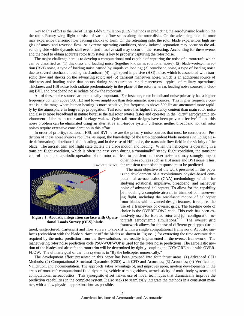
The main objective of the work presented in this paperis the development of a revolutionary physics-based com-putational aeroacoustics (CAA) methodology suitable forstudying rotational, impulsive, broadband, and maneuvernoise of advanced helicopters. To allow for the capabilityof modeling a complete aircraft in trimmed or maneuver-ing flight, including the aeroelastic motion of helicopterrotor blades with advanced design features, it requires theuse of a framework of overset grids. The baseline code ofchoice is the OVERFLOW2 code. This code has been ex-tensively used for isolated rotor and full configuration ro-torcraft aerodynamic simulations.4,5,6,7 The overset gridframework allows for the use of different grid types (struc-

tured, unstructured, Cartesian) and flow solvers to coexist within a single computational framework. Acoustic sur-faces (coincident with the blade surface or off the blades as shown in Figure 1) for extracting the time accurate datarequired by the noise prediction from the flow solutions are readily implemented in the overset framework. Themaneuvering rotor noise prediction code PSU-WOPWOP is used for the rotor noise predictions. The aeroelastic mo-tion of the blades and aircraft and rotor trim will be determined by tightly coupling the DYMORE code with OVER-FLOW. The ultimate goal of the this system is to “fly the helicopter numerically.”

The development effort presented in this paper has been grouped into four thrust areas: (1) Advanced CFDMethods; (2) Computational Structural Dynamics (CSD) with CFD and Acoustics; (3) Acoustics; (4) Verification,Validation, and Documentation. The approach takes advantage of, and improves upon, modern developments in theareas of rotorcraft computational fluid dynamics, vehicle trim algorithms, aeroelasticity of multi-body systems, andcomputational aeroacoustics. This synergistic effort makes use of novel techniques that dramatically improve theprediction capabilities in the complete system. It also seeks to seamlessly integrate the methods in a consistent man-ner, with as few physical approximations as possible.


Figure 1: Acoustic integration surface with Opera-tional Loads Survey (OLS) blade.

Kirchoff Surface

II. Methodology

Thrust 1: Advanced CFD Methods

The kernel CFD software is the OVERFLOW code version 2.0 by Buning, et.al.8 with elastic blade motion capa-bility as implemented per Nygaard9 . The goal of the advanced CFD methods thrust is the development of an un-steady aerodynamics method that enables more accurate rotorcraft performance and noise predictions for innovativequiet rotor designs. These new designs may utilize combinations of arbitrary planform/airfoil shapes, active and pas-sive flow control devices and novel blade control. Although the baseline OVERFLOW2 code has many of the de-sired computational features needed for this challenge, there remains the need for enhancements in turbulence mod-eling to more accurately capture the flow physics and to properly transport the pertinent flow quantities to an acous-tic data surface where other methods can determine the far-field noise. Advanced turbulence simulation methods andthe need to more accurately convect rotor-shed wakes without significantly increasing computational costs, particu-lar from within an aircraft design cycle, calls for the need for higher-order methods. Although the structured oversetgrid capability within OVERFLOW has the capability of handling very complex geometric shapes and to adapt tooff body flow features, other Cartesian based methods may prove to be more cost effective and accurate for the chal-lenge.

Turbulence ModelingIt is imperative that the unsteady physics of both the flow field and the blade surface be correctly predicted. The

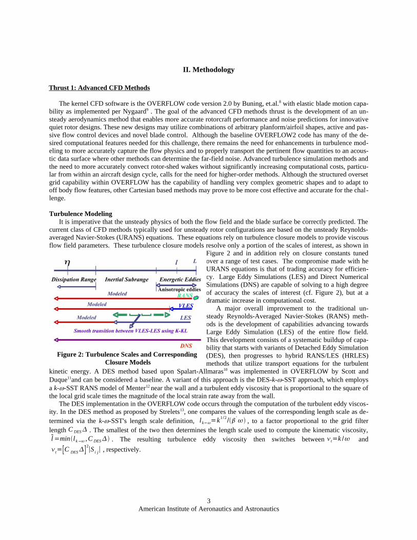
current class of CFD methods typically used for unsteady rotor configurations are based on the unsteady Reynolds-averaged Navier-Stokes (URANS) equations. These equations rely on turbulence closure models to provide viscousflow field parameters. These turbulence closure models resolve only a portion of the scales of interest, as shown in

Figure 2 and in addition rely on closure constants tunedover a range of test cases. The compromise made with heURANS equations is that of trading accuracy for efficien-cy. Large Eddy Simulations (LES) and Direct NumericalSimulations (DNS) are capable of solving to a high degreeof accuracy the scales of interest (cf. Figure 2), but at adramatic increase in computational cost.

A major overall improvement to the traditional un-steady Reynolds-Averaged Navier-Stokes (RANS) meth-ods is the development of capabilities advancing towardsLarge Eddy Simulation (LES) of the entire flow field.This development consists of a systematic buildup of capa-bility that starts with variants of Detached Eddy Simulation(DES), then progresses to hybrid RANS/LES (HRLES)methods that utilize transport equations for the turbulent

kinetic energy. A DES method based upon Spalart-Allmaras10 was implemented in OVERFLOW by Scott andDuque11and can be considered a baseline. A variant of this approach is the DES-k-ω-SST approach, which employsa k-ω-SST RANS model of Menter12 near the wall and a turbulent eddy viscosity that is proportional to the square ofthe local grid scale times the magnitude of the local strain rate away from the wall.

The DES implementation in the OVERFLOW code occurs through the computation of the turbulent eddy viscos-ity. In the DES method as proposed by Strelets13, one compares the values of the corresponding length scale as de-termined via the k-ω-SST's length scale definition, l k=k1 /2/ ' , to a factor proportional to the grid filterlength C DES . The smallest of the two then determines the length scale used to compute the kinematic viscosity,l =minl k ,C DES . The resulting turbulence eddy viscosity then switches between t=k / andt=[C DES ]2∣Si j∣ , respectively.


Figure 2: Turbulence Scales and Corresponding Closure Models

These DES models are improved via a hybrid RANS-LES (HRLES) method that eliminates assumptions inthe flow away from the near wall region. The HRLES method implemented in this project follows the implementa-tion of the XLES method by Kok et al.14. The HRLES method utilizes the same near-wall k-ω-SST RANS turbu-lence model as the DES method to affect a consistent comparison. The DES-k-ω−SST method assumes local equi-librium to approach the Smagorinsky algebraic model. This assumption is not strictly valid and is not likely to occurin these applications. In the HRLES method, away from the wall, this assumption is not made, and thus it becomesa true LES using the subgrid kinetic energy model. The length scale for the HRLES method is determined from theminimum of two values: l =min k / ,C1 . As a result, away from the wall the turbulent viscosity blends fromt=k / to t=C1 k . This method extends the capability of the k-ω-SST RANS over a larger range of scales

(cf. Fig. 2), and thus will capture the unsteady characteristics of the flow field more accurately than its RANS coun-terpart, as demonstrated by Shelton et al.15 For coarser grids, the HRLES method is equivalent to a very large eddysimulation (VLES).

The most advanced turbulence model investigated in this project is known as KES (kinetic eddy simulation) anddiffers considerably from the preceding hybrid methods. The KES method directly estimates the local unresolved ki-netic energy (k) and the local characteristic length scale l corresponding to this unresolved kinetic energy via the so-lution of the two transport equations for k and for k-l. Unlike DES-k-ω−SST and HRLES, KES does not make an apriori assumption about the local length scale, even in the near-wall region. Both k and l evolve locally as part of thesolution via the two transport equations. KES is an LES methodology, but in the case where the local grid resolu-tion is inadequate, KES smoothly transitions to a Very Large Eddy Simulation (VLES) where only the very largestscales are resolved. The ability to smoothly transition from LES to VLES is a unique feature of the KES model,which can be considered a VLES-LES model. Furthermore, there is no a priori assignment of where VLES or LESdominates since the transition between the two methods occurs naturally as a part of the solution. KES is a signifi-cant departure from the strategies in either DES-k-w−SST or HRLES. An earlier implementation of KES was appliedto free shear flows, see Arunajatesan16, and has been extended to unsteady motion of curvilinear grids for this appli-cation.17 A significant portion of the effort lies in the ability to port the KES method into existing RANS based codestructures, many of which rely on various strategies of algorithm simplification to increase code efficiency.

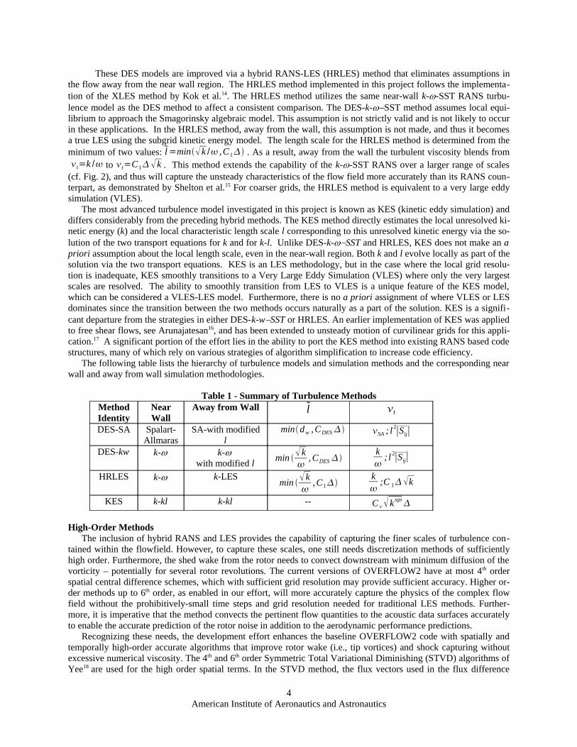
The following table lists the hierarchy of turbulence models and simulation methods and the corresponding nearwall and away from wall simulation methodologies.

Table 1 - Summary of Turbulence MethodsMethodIdentity

NearWall

Away from Wall l t

DES-SA Spalart-Allmaras

SA-with modifiedl

min dw , CDES SA ; l 2∣Sij∣

DES-kw k-ω k-ω with modified l min k

, CDES

k

; l 2∣Sij∣

HRLES k-ω k-LES min k

, C1k

;C 1 k

KES k-kl k-kl -- C ksgs

High-Order MethodsThe inclusion of hybrid RANS and LES provides the capability of capturing the finer scales of turbulence con-

tained within the flowfield. However, to capture these scales, one still needs discretization methods of sufficientlyhigh order. Furthermore, the shed wake from the rotor needs to convect downstream with minimum diffusion of thevorticity – potentially for several rotor revolutions. The current versions of OVERFLOW2 have at most 4th orderspatial central difference schemes, which with sufficient grid resolution may provide sufficient accuracy. Higher or-der methods up to 6th order, as enabled in our effort, will more accurately capture the physics of the complex flowfield without the prohibitively-small time steps and grid resolution needed for traditional LES methods. Further-more, it is imperative that the method convects the pertinent flow quantities to the acoustic data surfaces accuratelyto enable the accurate prediction of the rotor noise in addition to the aerodynamic performance predictions.

Recognizing these needs, the development effort enhances the baseline OVERFLOW2 code with spatially andtemporally high-order accurate algorithms that improve rotor wake (i.e., tip vortices) and shock capturing withoutexcessive numerical viscosity. The 4th and 6th order Symmetric Total Variational Diminishing (STVD) algorithms ofYee18 are used for the high order spatial terms. In the STVD method, the flux vectors used in the flux difference


evaluations are viewed as the sum of two parts – the physical flux that is always symmetrically computed and a nu-merical viscosity or diffusion term. The symmetric part uses fourth- and sixth-order symmetric schemes while thenumerical viscosity term is computed by using either a 3rd order MUSCL scheme or 3rd or 5th order Weighted Essen-tially Non-Oscillatory Scheme (WENO). Details for the STVD flux vector evaluations and the WENO stencils im-plemented for this effort are presented in the dissertation by Usta.19

Cartesian Grid MethodsThe OVERFLOW2 code currently utilizes curvilinear body-fitting grids, which overlap (or overset) uniform

Cartesian grids that carry the solution to the far field. The overset structured body fitting grids can move and deformwith the body motion and have proven useful in modeling rather complex geometries. However, the types of controldevices and complex shapes that may be utilized for a quiet rotor may prove to be too complicated for even oversetstructured grids. Even though the body-fitted structured grids have proven useful, they still take considerable effortto generate.

The overset uniform Cartesian grids capability in OVERFLOW2 provides minimum solution error and simplifiesboth grid generation and load balancing issues associated with distributed parallel computing. The Cartesian back-ground grid can also be used to adapt on the solution and minimize diffusion of flow features such as wakes andshocks. However, the uniform Cartesian grids do have some disadvantages. Firstly, because the grids are uniformlyfine throughout, a typical first level grid (the uniform Cartesian grid closest to the near body grid) can become verylarge (in terms of the number of grid points) and may be very fine in spatial areas where the refinement is not need-ed. Secondly, using the uniform overset Cartesian grids in a solution adaptation mode may lead to an excessivenumber of overset grids; each of which needs to interpolate the information as it is transferred between the overlap-ping grids, resulting in an overall degraded solution quality.

To overcome these limitations, the current effort introduces two very different Cartesian grid methods. One is animmersed boundary method designed to simplify the simulation of very complex body shapes and deformations.The other method is an unstructured Cartesian method that provides a more efficient off-body grid adaptation capa-bility for shed wakes and shock waves.

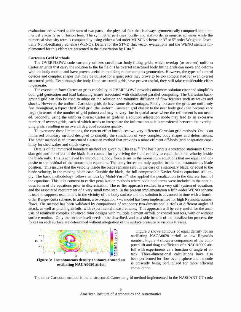
Details of the immersed boundary method are given by Cho et al.20 The basic grid is a stretched stationary Carte-sian grid and the effect of the blade is accounted for by driving the fluid velocity to equal the blade velocity insidethe blade only. This is achieved by introducing body force terms in the momentum equations that are equal and op-posite to the residual of the momentum equations. The body forces are only applied inside the instantaneous bladeposition. This insures that the velocity inside the blade remains zero, in the case of a stationary blade, or equal to theblade velocity, in the moving blade case. Outside the blade, the full compressible Navier-Stokes equations still ap-ply. The basic methodology follows an idea by Mohd-Yusof21 who applied the penalization to the discrete form ofthe equations. This is in contrast to earlier penalization methods where additional terms were included in the contin-uous form of the equations prior to discretization. The earlier approach resulted in a very stiff system of equationsand the associated requirement of a very small time step. In the present implementation a fifth-order WENO schemeis used to suppress oscillations in the vicinity of the body surface and the solution is advanced in time with a fourth-order Runge-Kutta scheme. In addition, a two-equation k−ω model has been implemented for high Reynolds numberflows. The method has been validated by comparisons of stationary two-dimensional airfoils at different angles ofattack, as well as pitching airfoils, with experimental measurements. This approach will be very useful for the anal-ysis of relatively complex advanced rotor designs with multiple element airfoils or control surfaces, with or withoutsurface motion. Only the surface itself needs to be described, and as a side benefit of the penalization process, theforces on each surface are determined without integration of the surface pressure or viscous stresses.

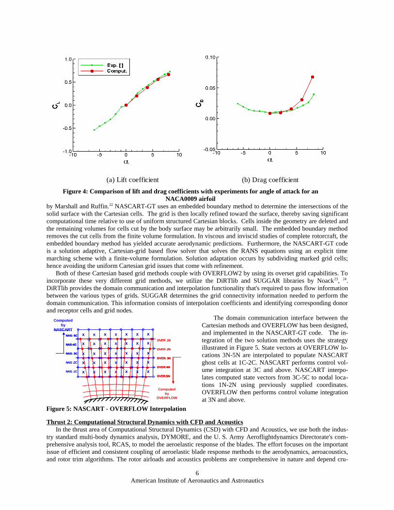
Figure 3 shows contours of equal density for anoscillating NACA0020 airfoil at low Reynoldsnumber. Figure 4 shows a comparison of the com-puted lift and drag coefficients of a NACA0009 air-foil with experiments as a function of angle of at-tack. Three-dimensional calculations have alsobeen performed for flow over a sphere and the codeis presently being parallelized for more efficientcomputation.

The other Cartesian method is the unstructured Cartesian grid method implemented in the NASCART-GT code


Figure 3: Instantaneous density contours around an oscillating NACA0020 airfoil

by Marshall and Ruffin.22 NASCART-GT uses an embedded boundary method to determine the intersections of thesolid surface with the Cartesian cells. The grid is then locally refined toward the surface, thereby saving significantcomputational time relative to use of uniform structured Cartesian blocks. Cells inside the geometry are deleted andthe remaining volumes for cells cut by the body surface may be arbitrarily small. The embedded boundary methodremoves the cut cells from the finite volume formulation. In viscous and inviscid studies of complete rotorcraft, theembedded boundary method has yielded accurate aerodynamic predictions. Furthermore, the NASCART-GT codeis a solution adaptive, Cartesian-grid based flow solver that solves the RANS equations using an explicit timemarching scheme with a finite-volume formulation. Solution adaptation occurs by subdividing marked grid cells;hence avoiding the uniform Cartesian grid issues that come with refinement.

Both of these Cartesian based grid methods couple with OVERFLOW2 by using its overset grid capabilities. Toincorporate these very different grid methods, we utilize the DiRTlib and SUGGAR libraries by Noack23, 24.DiRTlib provides the domain communication and interpolation functionality that's required to pass flow informationbetween the various types of grids. SUGGAR determines the grid connectivity information needed to perform thedomain communication. This information consists of interpolation coefficients and identifying corresponding donorand receptor cells and grid nodes.

The domain communication interface between theCartesian methods and OVERFLOW has been designed,and implemented in the NASCART-GT code. The in-tegration of the two solution methods uses the strategyillustrated in Figure 5. State vectors at OVERFLOW lo-cations 3N-5N are interpolated to populate NASCARTghost cells at 1C-2C. NASCART performs control vol-ume integration at 3C and above. NASCART interpo-lates computed state vectors from 3C-5C to nodal loca-tions 1N-2N using previously supplied coordinates.OVERFLOW then performs control volume integrationat 3N and above.

Thrust 2: Computational Structural Dynamics with CFD and AcousticsIn the thrust area of Computational Structural Dynamics (CSD) with CFD and Acoustics, we use both the indus-

try standard multi-body dynamics analysis, DYMORE, and the U. S. Army Aeroflightdynamics Directorate's com-prehensive analysis tool, RCAS, to model the aeroelastic response of the blades. The effort focuses on the importantissue of efficient and consistent coupling of aeroelastic blade response methods to the aerodynamics, aeroacoustics,and rotor trim algorithms. The rotor airloads and acoustics problems are comprehensive in nature and depend cru-


Figure 4: Comparison of lift and drag coefficients with experiments for angle of attack for anNACA0009 airfoil

(a) Lift coefficient (b) Drag coefficient

OVER: 1N

OVER: 2N

OVER: 3N

OVER:4N

OVER:5N

NAS: 5C

NAS:4C

NAS: 3C

NAS: 2C

NAS: 1C

Computedby

NASCART

Computedby

OVERFLOW

X

X

X

X

X

X

X

X

X

X

X

X

X

X

X

X

X

X

X

X

X

X

X

X

X

X

X

X

X

X

X

X

X

X

X

OVER: 1N

OVER: 2N

OVER: 3N

OVER:4N

OVER:5N

NAS: 5C

NAS:4C

NAS: 3C

NAS: 2C

NAS: 1C

Computedby

NASCART

Computedby

OVERFLOW

OVER: 1N

OVER: 2N

OVER: 3N

OVER:4N

OVER:5N

NAS: 5C

NAS:4C

NAS: 3C

NAS: 2C

NAS: 1C

Computedby

NASCART

Computedby

OVERFLOW

X

X

X

X

X

X

X

X

X

X

X

X

X

X

X

X

X

X

X

X

X

X

X

X

X

X

X

X

X

X

X

X

X

X

X

X

X

X

X

X

X

X

X

X

X

X

X

X

X

X

X

X

X

X

X

X

X

X

X

X

X

X

X

X

X

X

X

X

X

X

X

X

X

X

X

X

X

X

X

X

X

X

X

X

X

X

X

X

X

X

X

X

X

X

X

X

X

X

X

X

Figure 5: NASCART - OVERFLOW Interpolation

cially on aircraft trim, rotor trim, and blade aeroelasticity. Hence, this thrust area couples the CFD methodologies(OVERFLOW) with rotorcraft comprehensive analysis (DYMORE) and noise prediction (PSU-WOPWOP) tools, toobtain fully integrated, aeroelastic and acoustic predictions.

Generic interfaces transfer data between the CFD and CSD. The interfaces need to be generic and documentedso that alternate codes can be used. The DYMORE, our primary CSD tool, uses an interface that is compatible withthe RCAS/OVERFLOW coupling standard currently in development at NASA/AFDD25; RCAS is used as a sec-ondary CSD tool in this project. The development effort employs a “two-pronged” approach to the CFD/CSD cou-pling: tight and loose coupling. Although the interfaces are somewhat different for tight and loose coupling strate-gies, they both must pass blade airload and surface position (trim and deformation) information between the CFDand the CSD codes.

Tight coupling is one methodology for solving equations of aeroelastic systems.26, 27 The tight coupling ap-proach is a time marching scheme that exchanges information between computational domains at each time step. Acommon time step is selected to insure accuracy and stability of both CFD and CSD algorithms. Tight coupling is avery general algorithm and can be applied to steady or transient flight conditions (maneuvers). The methodology isnecessary for transient maneuvers, but is currently computationally expensive for modeling steady flight conditions.Tight coupling may improve the quality of solutions needed for capturing complex behavior, such as dynamic stall,which also occurs for certain steady flight conditions. DYMORE is the primary CSD code that is tightly-coupled toOVERFLOW through generic interfaces. DYMORE28 calculates the blade response in the time-domain, and is well-suited for a tight-coupling with CFD. At every time step, the section positions and velocities are used to update theCFD grid; section forces and moments are used to predict the structural response. A preliminary coupling of DY-MORE with OVERFLOW was also developed26 .

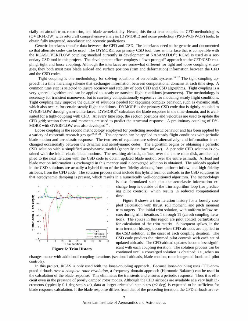
Loose coupling is the second methodology employed for predicting aeroelastic behavior and has been applied bya variety of rotorcraft research groups29 ,30 ,31 . The approach can be applied to steady flight conditions with periodicblade motion and aeroelastic response. The two sets of equations are solved alternatively, and information is ex-changed occasionally between the dynamic and aerodynamic codes. The algorithm begins by obtaining a periodicCSD solution with a simplified aerodynamic model (generally uniform inflow). A periodic CFD solution is ob-tained with the initial elastic blade motions. The resulting airloads, defined over the entire rotor disk, are then ap-plied to the next iteration with the CSD code to obtain updated blade motion over the entire azimuth. Airload andblade motion information is exchanged in this manner until a converged solution is obtained. The airloads appliedin the CSD solutions are actually a hybrid form of the low-fidelity airloads, from uniform inflow, and high fidelityairloads, from the CFD code. The solution process must include this hybrid form of airloads in the CSD solutions sothat aerodynamic damping is present, which results in a numerically well-conditioned algorithm. The methodology

is also formulated such that the aeroelastic information ex-change loop is outside of the trim algorithm loop (for predict-ing pilot controls), which results in reduced computationaltime.

Figure 6 shows a trim iteration history for a loosely cou-pled calculation with thrust, roll moment, and pitch momenttrim targets. The initial trim solution, with uniform inflow oc-curs during trim iterations 1 through 11 (zeroth coupling itera-tion). The spikes in this region are pilot control perturbationsfor calculation of the trim matrix. Subsequent spikes, in thetrim iteration history, occur when CFD airloads are applied tothe CSD solution, at the onset of each coupling iteration. TheCSD code predicts the trimmed pilot controls with each set ofupdated airloads. The CFD airload updates become less signif-icant with each coupling iteration. The solution process can becontinued until a converged solution is obtained; i.e., when no

changes occur with additional coupling iterations (sectional airloads, blade motion, rotor integrated loads and pilotcontrols).

In this project, RCAS is only used with the loose-coupling approach. Because loose-coupling uses CFD-com-puted airloads over a complete rotor revolution, a frequency domain approach (Harmonic Balance) can be used inthe calculation of the blade response. This eliminates the transients and ensures a periodic response. Thus it is effi-cient even in the presence of poorly damped rotor modes. Although the CFD airloads are available at a very high in-crements (typically 0.1 deg step size), data at larger azimuthal step sizes (~2 deg) is expected to be sufficient forblade response calculation. If the blade response differs from that of the preceding iteration, the CFD airloads are re-


Figure 6: Trim History

computed using the current blade motions, until convergence occurs.Vehicle orientation and blade positions affect both aerodynamics and aeroacoustics; hence, the coupling technol-

ogy has the potential for fundamentally revolutionizing simulation methods of maneuvering rotorcraft. The methodsdeveloped here also allow for the aeroelastic simulation of next generation rotors equipped with slots, slats, tip de-vices, and flaps.

Thrust 3: AcousticsThe ultimate and the main goal of this project is to provide a tool to develop helicopter rotors with dramatically

reduced rotor noise without sacrificing flight performance. The rotor noise prediction code PSU-WOPWOP, devel-oped by Brentner et al.,32, 33is the final element required to fulfill this goal. The PSU-WOPWOP code is a source-time dominant implementation of Farassat’s retarded-time formulation 1A34 of the Ffowcs Williams–Hawkings(FW–H) equation35, which is capable of predicting the rotor noise from multiple rotors for both steady and maneuverflight conditions. PSU-WOPWOP includes a chordwise-compact loading formulation (which can predict noisebased on section loading), a permeable surface implementation (which can account for the transonic effects associat-ed with high-speed-impulsive noise prediction or flow through the surface), as well as the traditional solid surfaceimplementation (which is appropriate for computing thickness and loading noise, BVI noise, and broadband noisesources).

Due to the potential importance of HSI noise, permeable acoustic data surfaces are used for most noise predic-tions in this project. These off-blade acoustic data surfaces are generated and included in the list of overset grids.Two types of permeable acoustic data surfaces will be used: 1) rotating – a surface which encloses each blade andthe transonic flow around it; and 2) non-rotating – a surface which encloses the entire rotor and translates with theaircraft. The advantage of the rotating acoustic data surface is that it is closer to the blade surface; hence, the CFDsolver does not have to maintain solution accuracy much farther than a few chords away from the blade surface.The rototating surfaces have a major drawback, however. The surface motion becomes supersonic if the surface ex-tends much beyond the blade tip. The retarded-time formulation 1A suffers from a Doppler singularity in this situa-tion. The nonrotating surface has the advantage that the surface motion is well below sonic speed, hence theDoppler singularity is not a concern and the surface can be extended as far from the blade tip as is necessary for ac-curate HSI noise predictions. The placement of the surface far from the rotor blades results in a much higher de-mand for computational accuracy in the flow field from the CFD code.

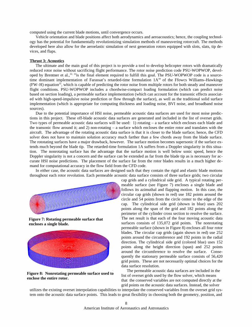
In either case, the acoustic data surfaces are designed such that they contain the rigid and elastic blade motionsthroughout each rotor revolution. Each permeable acoustic data surface consists of three surface grids; two circular

cap grids and a cylindrical side grid. A typical rotating per-meable surface (see Figure 7) encloses a single blade andfollows its azimuthal and flapping motion. In this case, thecircular cap grids (shown in red) use 182 points around thecircle and 54 points from the circle center to the edge of thecap. The cylindrical side grid (shown in blue) uses 202points along the span of the grid and 182 points along theperimeter of the cylinder cross section to resolve the surface.The net result is that each of the four moving acoustic datasurfaces consists of 135,072 grid points. The nonrotatingpermeable surface (shown in Figure 8) encloses all four rotorblades. The circular cap grids (again shown in red) use 252points around the circumference and 192 points in the radialdirection. The cylindrical side grid (colored blue) uses 152points along the height direction (span) and 252 pointsaround the circumference to resolve the surface. Conse-quently the stationary permeable surface consists of 56,420grid points. These are not necessarily optimal choices for thedata surface resolution.

The permeable acoustic data surfaces are included in thelist of overset grids used by the flow solver, which meansthat the conserved variables are not computed directly at thegrid points on the acoustic data surfaces. Instead, the solver

utilizes the existing overset interpolation capabilities to interpolate the conserved variables from the overset grid sys-tem onto the acoustic data surface points. This leads to great flexibility in choosing both the geometry, position, and


Figure 7: Rotating permeable surface that encloses a single blade.

Figure 8: Nonrotating permeable surface used to enclose the entire rotor.

resolution of the acoustic data surface, but care must be taken to ensure that the overset grids accurately carry the so-lution to the acoustic data surfaces.

III. Preliminary ResultsUnder Thrust 4, the primary software development, verification, and validation efforts utilize a series of well-es-

tablished experiments designed for helicopter related flowfields. These experiments include static stall and dynamicstall of NACA0015 airfoil by Pizialli36 . In addition, full rotor demonstration computations shall be used to verifyand validate the integrated methods. The benchmark data include experimental data derived from the UH-60A rotor-craft flight test37 , model rotor tested in the DNW38 , and the HART39 and HART-II40 rotor tests . These experimentsinclude rotors in high-speed forward and descent flight conditions, which enable the systematic validation of all thecomponent technologies. This section presents a snapshot of early and preliminary results that demonstrate the noiseprediction system enhancements – high order methods, turbulence modeling, adaptive Cartesian method, and noiseprediction for elastic rotors.

In-conjunction with full rotor computations, several test cases were performed to verify the implementation ofthe new methodologies. These computationsincluded simple vortex convection computa-tions and airfoils operating in dynamic stallconditions to verify the implementation ofthe higher-order methods. Additional wingand airfoil stall computations were per-formed in concert with the higher-ordermethods to to verify the turbulent modelingmethods.

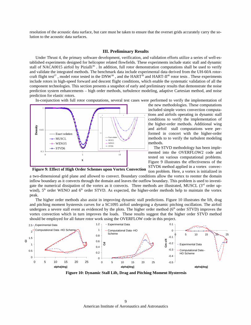
The STVD methodology has been imple-mented into the OVERFLOW2 code andtested on various computational problems.Figure 9 illustrates the effectiveness of theSTVD6 method applied in a vortex convec-tion problem. Here, a vortex is initialized in

a two-dimensional grid plane and allowed to convect. Boundary conditions allow the vortex to reenter the domaininflow boundary as it convects through the domain and leaves the outflow boundary. This problem is used to investi-gate the numerical dissipation of the vortex as it convects. Three methods are illustrated, MUSCL (3rd order up-wind), 5th order WENO and 6th order STVD. As expected, the higher-order methods help to maintain the vortexpeak.

The higher order methods also assist in improving dynamic stall predictions. Figure 10 illustrates the lift, dragand pitching moment hysteresis curves for a SC1095 airfoil undergoing a dynamic pitching oscillation. The airfoilundergoes a severe stall event as evidenced by the plots. The higher order method (6th order STVD) improves thevortex convection which in turn improves the loads. These results suggest that the higher order STVD methodshould be employed for all future rotor work using the OVERFLOW code in this project.


Figure 9: Effect of High Order Schemes upon Vortex Convection

0.3

0.65

1

0 5 10

x

Den

sity

Exact solutionMUSCLWENO5STVD6 0.3

0.4

0.54 5 6

Exact solutionMUSCLWENO5STVD6

Figure 10: Dynamic Stall Lift, Drag and Pitching Moment Hysteresis

0

0.5

1

1.5

2

2.5

0 5 10 15 20 25alpha[deg]

Cl

Experimental Data

Computational Data -HO Scheme

0

0.2

0.4

0.6

0.8

1

1.2

0 5 10 15 20 25

alpha[deg]

Cd

Experimental Data

Computational Data -HOScheme

-0.5

-0.4

-0.3

-0.2

-0.1

0

0.1

0 5 10 15 20 25

alpha[deg]

Cm

c/4

Experimental Data

Computational Data -HO Scheme

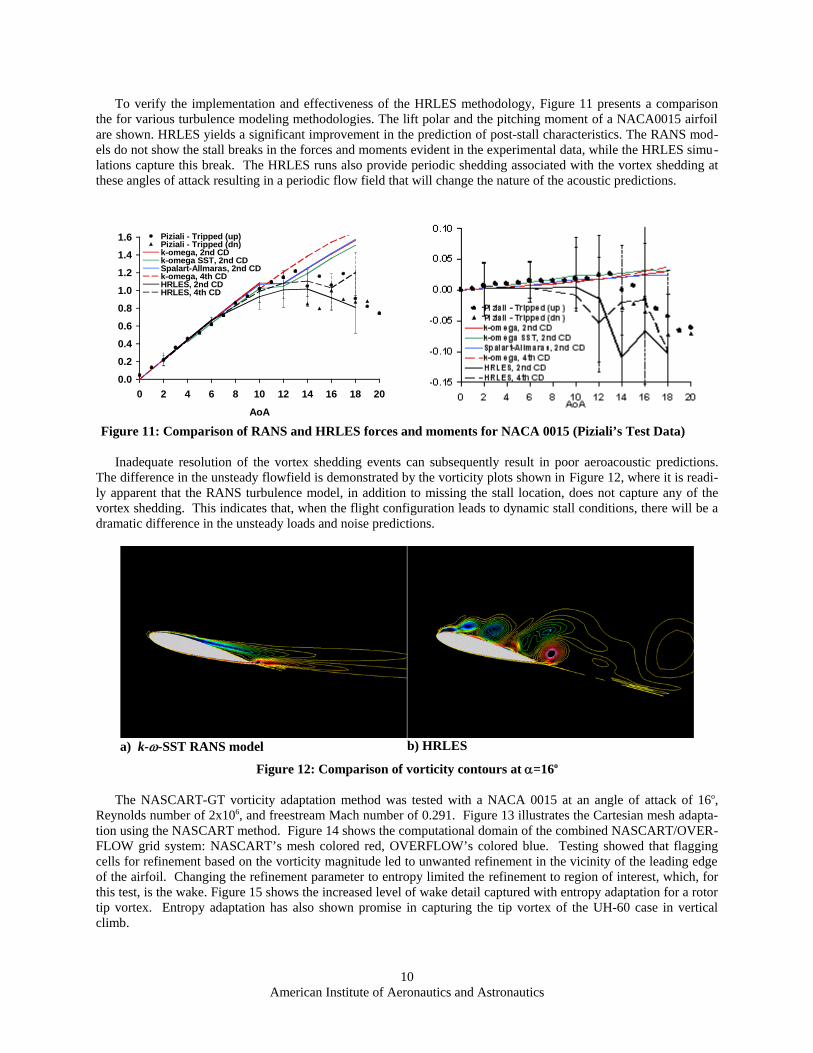
To verify the implementation and effectiveness of the HRLES methodology, Figure 11 presents a comparisonthe for various turbulence modeling methodologies. The lift polar and the pitching moment of a NACA0015 airfoilare shown. HRLES yields a significant improvement in the prediction of post-stall characteristics. The RANS mod-els do not show the stall breaks in the forces and moments evident in the experimental data, while the HRLES simu-lations capture this break. The HRLES runs also provide periodic shedding associated with the vortex shedding atthese angles of attack resulting in a periodic flow field that will change the nature of the acoustic predictions.

Inadequate resolution of the vortex shedding events can subsequently result in poor aeroacoustic predictions.The difference in the unsteady flowfield is demonstrated by the vorticity plots shown in Figure 12, where it is readi-ly apparent that the RANS turbulence model, in addition to missing the stall location, does not capture any of thevortex shedding. This indicates that, when the flight configuration leads to dynamic stall conditions, there will be adramatic difference in the unsteady loads and noise predictions.

a) k-ω-SST RANS model b) HRLES

Figure 12: Comparison of vorticity contours at α=16o

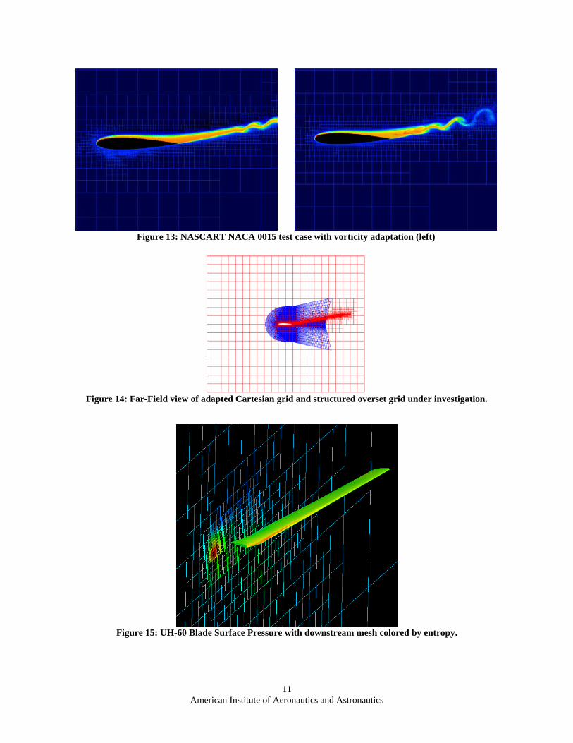
The NASCART-GT vorticity adaptation method was tested with a NACA 0015 at an angle of attack of 16o,Reynolds number of 2x106, and freestream Mach number of 0.291. Figure 13 illustrates the Cartesian mesh adapta-tion using the NASCART method. Figure 14 shows the computational domain of the combined NASCART/OVER-FLOW grid system: NASCART’s mesh colored red, OVERFLOW’s colored blue. Testing showed that flaggingcells for refinement based on the vorticity magnitude led to unwanted refinement in the vicinity of the leading edgeof the airfoil. Changing the refinement parameter to entropy limited the refinement to region of interest, which, forthis test, is the wake. Figure 15 shows the increased level of wake detail captured with entropy adaptation for a rotortip vortex. Entropy adaptation has also shown promise in capturing the tip vortex of the UH-60 case in verticalclimb.


Figure 11: Comparison of RANS and HRLES forces and moments for NACA 0015 (Piziali’s Test Data)

0.0

0.2

0.4

0.6

0.8

1.0

1.2

1.4

1.6

0 2 4 6 8 10 12 14 16 18 20

AoA

Piziali - Tripped (up)Piziali - Tripped (dn)k-omega, 2nd CDk-omega SST, 2nd CDSpalart-Allmaras, 2nd CDk-omega, 4th CDHRLES, 2nd CDHRLES, 4th CD


Figure 13: NASCART NACA 0015 test case with vorticity adaptation (left)

Figure 14: Far-Field view of adapted Cartesian grid and structured overset grid under investigation.

Figure 15: UH-60 Blade Surface Pressure with downstream mesh colored by entropy.

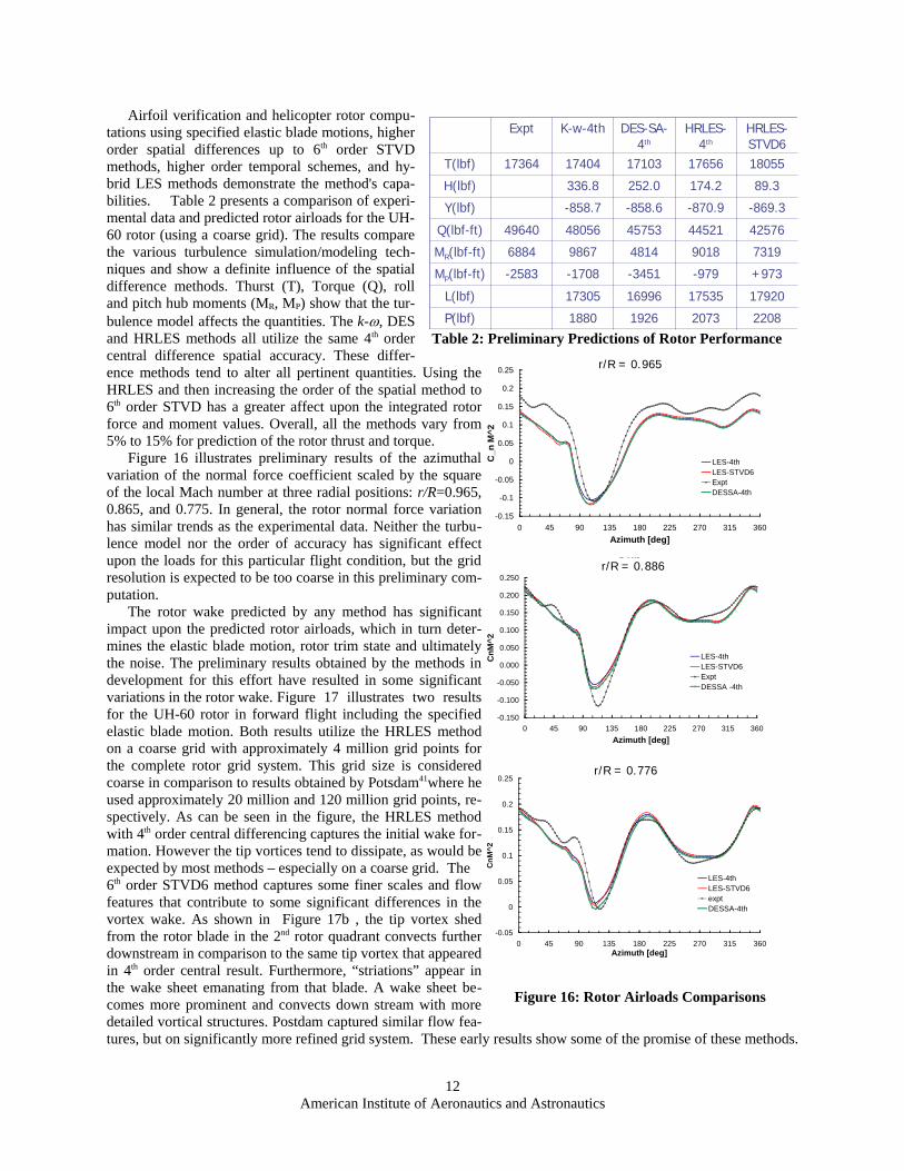
Airfoil verification and helicopter rotor compu-tations using specified elastic blade motions, higherorder spatial differences up to 6th order STVDmethods, higher order temporal schemes, and hy-brid LES methods demonstrate the method's capa-bilities. Table 2 presents a comparison of experi-mental data and predicted rotor airloads for the UH-60 rotor (using a coarse grid). The results comparethe various turbulence simulation/modeling tech-niques and show a definite influence of the spatialdifference methods. Thurst (T), Torque (Q), rolland pitch hub moments (MR, MP) show that the tur-bulence model affects the quantities. The k-ω, DESand HRLES methods all utilize the same 4th ordercentral difference spatial accuracy. These differ-ence methods tend to alter all pertinent quantities. Using theHRLES and then increasing the order of the spatial method to6th order STVD has a greater affect upon the integrated rotorforce and moment values. Overall, all the methods vary from5% to 15% for prediction of the rotor thrust and torque.

Figure 16 illustrates preliminary results of the azimuthalvariation of the normal force coefficient scaled by the squareof the local Mach number at three radial positions: r/R=0.965,0.865, and 0.775. In general, the rotor normal force variationhas similar trends as the experimental data. Neither the turbu-lence model nor the order of accuracy has significant effectupon the loads for this particular flight condition, but the gridresolution is expected to be too coarse in this preliminary com-putation.

The rotor wake predicted by any method has significantimpact upon the predicted rotor airloads, which in turn deter-mines the elastic blade motion, rotor trim state and ultimatelythe noise. The preliminary results obtained by the methods indevelopment for this effort have resulted in some significantvariations in the rotor wake. Figure 17 illustrates two resultsfor the UH-60 rotor in forward flight including the specifiedelastic blade motion. Both results utilize the HRLES methodon a coarse grid with approximately 4 million grid points forthe complete rotor grid system. This grid size is consideredcoarse in comparison to results obtained by Potsdam41where heused approximately 20 million and 120 million grid points, re-spectively. As can be seen in the figure, the HRLES methodwith 4th order central differencing captures the initial wake for-mation. However the tip vortices tend to dissipate, as would beexpected by most methods – especially on a coarse grid. The6th order STVD6 method captures some finer scales and flowfeatures that contribute to some significant differences in thevortex wake. As shown in Figure 17b , the tip vortex shedfrom the rotor blade in the 2nd rotor quadrant convects furtherdownstream in comparison to the same tip vortex that appearedin 4th order central result. Furthermore, “striations” appear inthe wake sheet emanating from that blade. A wake sheet be-comes more prominent and convects down stream with moredetailed vortical structures. Postdam captured similar flow fea-tures, but on significantly more refined grid system. These early results show some of the promise of these methods.


Figure 16: Rotor Airloads Comparisons

r/R=0.965

-0.15

-0.1

-0.05

0

0.05

0.1

0.15

0.2

0.25

0 45 90 135 180 225 270 315 360Azimuth [deg]

C_n

M^2

LES-4thLES-STVD6ExptDESSA-4th

r/R=0.865

-0.150

-0.100

-0.050

0.000

0.050

0.100

0.150

0.200

0.250

0 45 90 135 180 225 270 315 360Azimuth [deg]

CnM

^2

LES-4thLES-STVD6ExptDESSA -4th

r/R=0.775

-0.05

0

0.05

0.1

0.15

0.2

0.25

0 45 90 135 180 225 270 315 360Azimuth [deg]

CnM

^2

LES-4thLES-STVD6exptDESSA-4th

Table 2: Preliminary Predictions of Rotor Performance

4257644521457534805649640Q(lbf-ft)

73199018481498676884MR(lbf-ft)

+973-979-3451-1708-2583MP(lbf-ft)

1805517656171031740417364T(lbf)

2208207319261880P(lbf)

17920175351699617305L(lbf)

-869.3-870.9-858.6-858.7Y(lbf)

336.8

K-w-4th

H(lbf) 89.3174.2252.0

HRLES-STVD6

HRLES-4th

DES-SA-4th

Expt

r/R = 0.886

r/R = 0.776

r/R = 0.965

a) HRLES-4th Central b) HRLES-STVD6

Figure 17 - UH-60, Iso-Vorticity Surfaces

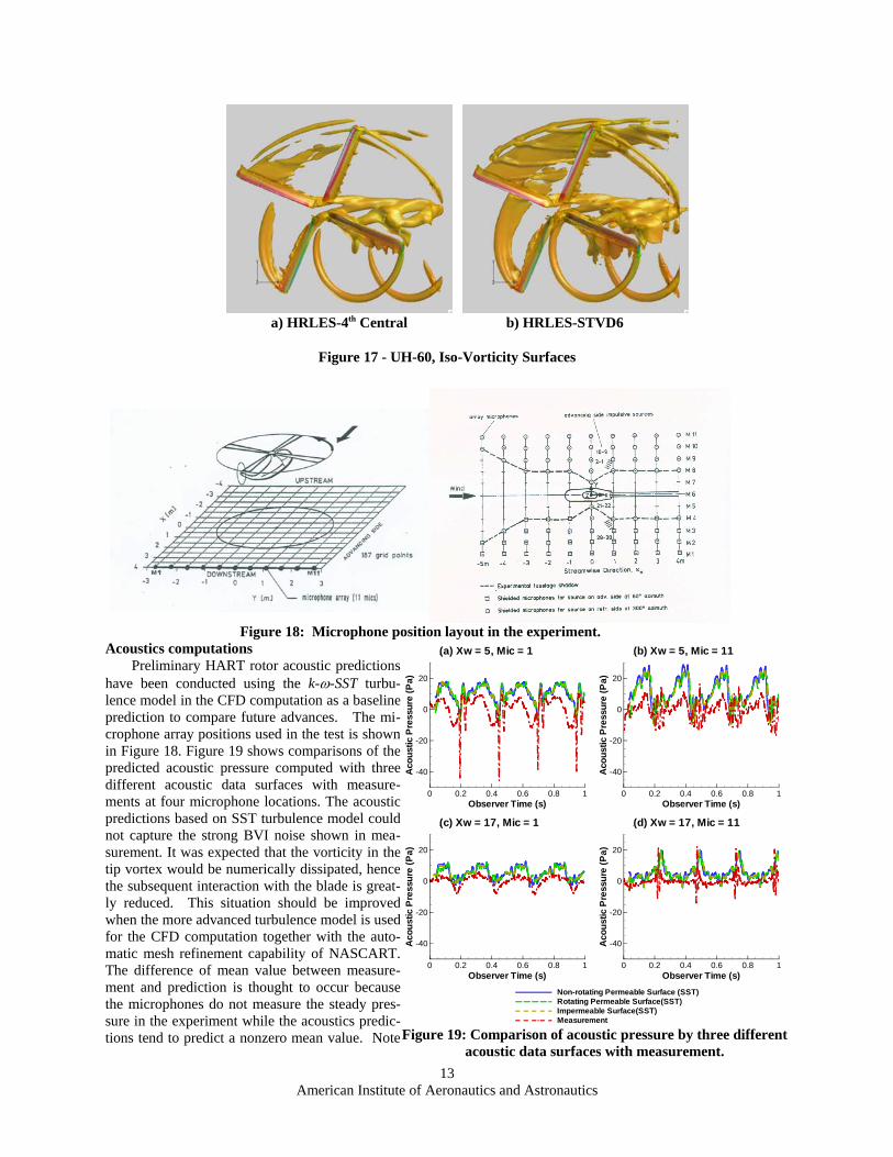
Acoustics computationsPreliminary HART rotor acoustic predictions

have been conducted using the k-ω-SST turbu-lence model in the CFD computation as a baselineprediction to compare future advances. The mi-crophone array positions used in the test is shownin Figure 18. Figure 19 shows comparisons of thepredicted acoustic pressure computed with threedifferent acoustic data surfaces with measure-ments at four microphone locations. The acousticpredictions based on SST turbulence model couldnot capture the strong BVI noise shown in mea-surement. It was expected that the vorticity in thetip vortex would be numerically dissipated, hencethe subsequent interaction with the blade is great-ly reduced. This situation should be improvedwhen the more advanced turbulence model is usedfor the CFD computation together with the auto-matic mesh refinement capability of NASCART.The difference of mean value between measure-ment and prediction is thought to occur becausethe microphones do not measure the steady pres-sure in the experiment while the acoustics predic-tions tend to predict a nonzero mean value. Note


Figure 18: Microphone position layout in the experiment.

Observer Time (s)

Aco

ustic

Pre

ssur

e(P

a)

0 0.2 0.4 0.6 0.8 1

-40

-20

0

20

A verag eTi meH istor y(Po le= 065x w= 5)

x= 2.0 0m, vtun= 33 .1,a tpp= 5.11 , rm ue=0 .15


x= -4.0 0m, vtun =33 .1,a tpp= 5.11 , rm ue=0 .15

Xw=5 ,Mic =#1

(b) Xw = 5, Mic = 11A verag eTi meH istor y(Po le= 065x w= 5)

x= 2.0 0m, vtun= 33 .1,a tpp= 5.11 , rm ue=0 .15


x= -4.0 0m, vtun =33 .1,a tpp= 5.11 , rm ue=0 .15

Xw=5 ,Mic =#1


x= 2.0 0m, vtun= 33 .1,a tpp= 5.11 , rm ue=0 .15


x= -4.0 0m, vtun =33 .1,a tpp= 5.11 , rm ue=0 .15

Xw=5 ,Mic =#1


x= 2.0 0m, vtun= 33 .1,a tpp= 5.11 , rm ue=0 .15


x= -4.0 0m, vtun =33 .1,a tpp= 5.11 , rm ue=0 .15

Xw=5 ,Mic =#1


x= 2.0 0m, vtun= 33 .1,a tpp= 5.11 , rm ue=0 .15


x= -4.0 0m, vtun =33 .1,a tpp= 5.11 , rm ue=0 .15


x= 2.0 0m, vtun= 33 .1,a tpp= 5.11 , rm ue=0 .15


x= -4.0 0m, vtun =33 .1,a tpp= 5.11 , rm ue=0 .15

Xw=5 ,Mic =#1


x= 2.0 0m, vtun= 33 .1,a tpp= 5.11 , rm ue=0 .15


x= -4.0 0m, vtun =33 .1,a tpp= 5.11 , rm ue=0 .15


x= 2.0 0m, vtun= 33 .1,a tpp= 5.11 , rm ue=0 .15


x= -4.0 0m, vtun =33 .1,a tpp= 5.11 , rm ue=0 .15


x= 2.0 0m, vtun= 33 .1,a tpp= 5.11 , rm ue=0 .15


x= -4.0 0m, vtun =33 .1,a tpp= 5.11 , rm ue=0 .15

Observer Time (s)

Aco

ustic

Pre

ssur

e(P

a)

0 0.2 0.4 0.6 0.8 1

-40

-20

0

20


x= 2.0 0m, vtun= 33 .1,a tpp= 5.11 , rm ue=0 .15


x= -4.0 0m, vtun =33 .1,a tpp= 5.11 , rm ue=0 .15

Xw =5,M ic= #1


x= 2.0 0m, vtun= 33 .1,a tpp= 5.11 , rm ue=0 .15


x= -4.0 0m, vtun =33 .1,a tpp= 5.11 , rm ue=0 .15

Xw =5,M ic= #1

(a) Xw = 5, Mic = 1A verag eTi meH istor y(Po le= 065x w= 5)

x= 2.0 0m, vtun= 33 .1,a tpp= 5.11 , rm ue=0 .15


x= -4.0 0m, vtun =33 .1,a tpp= 5.11 , rm ue=0 .15

Xw =5,M ic= #1


x= 2.0 0m, vtun= 33 .1,a tpp= 5.11 , rm ue=0 .15


x= -4.0 0m, vtun =33 .1,a tpp= 5.11 , rm ue=0 .15

Xw =5,M ic= #1


x= 2.0 0m, vtun= 33 .1,a tpp= 5.11 , rm ue=0 .15


x= -4.0 0m, vtun =33 .1,a tpp= 5.11 , rm ue=0 .15


x= 2.0 0m, vtun= 33 .1,a tpp= 5.11 , rm ue=0 .15


x= -4.0 0m, vtun =33 .1,a tpp= 5.11 , rm ue=0 .15

Xw =5,M ic= #1


x= 2.0 0m, vtun= 33 .1,a tpp= 5.11 , rm ue=0 .15


x= -4.0 0m, vtun =33 .1,a tpp= 5.11 , rm ue=0 .15


x= 2.0 0m, vtun= 33 .1,a tpp= 5.11 , rm ue=0 .15


x= -4.0 0m, vtun =33 .1,a tpp= 5.11 , rm ue=0 .15


x= 2.0 0m, vtun= 33 .1,a tpp= 5.11 , rm ue=0 .15


x= -4.0 0m, vtun =33 .1,a tpp= 5.11 , rm ue=0 .15

Observer Time (s)

Aco

ustic

Pre

ssur

e(P

a)

0 0.2 0.4 0.6 0.8 1

-40

-20

0

20


x= 2.0 0m, vtun= 33 .1,a tpp= 5.11 , rm ue=0 .15


x= -4.0 0m, vtun =33 .1,a tpp= 5.11 , rm ue=0 .15

Xw=5 ,Mic =#1


x= 2.0 0m, vtun= 33 .1,a tpp= 5.11 , rm ue=0 .15


x= -4.0 0m, vtun =33 .1,a tpp= 5.11 , rm ue=0 .15

Xw=5 ,Mic =#1


x= 2.0 0m, vtun= 33 .1,a tpp= 5.11 , rm ue=0 .15


x= -4.0 0m, vtun =33 .1,a tpp= 5.11 , rm ue=0 .15

Xw=5 ,Mic =#1

(d) Xw = 17, Mic = 11A verag eTi meH istor y(Po le= 065x w= 5)

x= 2.0 0m, vtun= 33 .1,a tpp= 5.11 , rm ue=0 .15


x= -4.0 0m, vtun =33 .1,a tpp= 5.11 , rm ue=0 .15

Xw=5 ,Mic =#1


x= 2.0 0m, vtun= 33 .1,a tpp= 5.11 , rm ue=0 .15


x= -4.0 0m, vtun =33 .1,a tpp= 5.11 , rm ue=0 .15


x= 2.0 0m, vtun= 33 .1,a tpp= 5.11 , rm ue=0 .15


x= -4.0 0m, vtun =33 .1,a tpp= 5.11 , rm ue=0 .15

Xw=5 ,Mic =#1


x= 2.0 0m, vtun= 33 .1,a tpp= 5.11 , rm ue=0 .15


x= -4.0 0m, vtun =33 .1,a tpp= 5.11 , rm ue=0 .15


x= 2.0 0m, vtun= 33 .1,a tpp= 5.11 , rm ue=0 .15


x= -4.0 0m, vtun =33 .1,a tpp= 5.11 , rm ue=0 .15


x= 2.0 0m, vtun= 33 .1,a tpp= 5.11 , rm ue=0 .15


x= -4.0 0m, vtun =33 .1,a tpp= 5.11 , rm ue=0 .15

Observer Time (s)

Aco

ustic

Pre

ssur

e(P

a)

0 0.2 0.4 0.6 0.8 1

-40

-20

0

20


x= 2.0 0m, vtun= 33 .1,a tpp= 5.11 , rm ue=0 .15


x= -4.0 0m, vtun =33 .1,a tpp= 5.11 , rm ue=0 .15

Xw =5,M ic= #1


x= 2.0 0m, vtun= 33 .1,a tpp= 5.11 , rm ue=0 .15


x= -4.0 0m, vtun =33 .1,a tpp= 5.11 , rm ue=0 .15

Xw =5,M ic= #1


x= 2.0 0m, vtun= 33 .1,a tpp= 5.11 , rm ue=0 .15


x= -4.0 0m, vtun =33 .1,a tpp= 5.11 , rm ue=0 .15

Xw =5,M ic= #1


x= 2.0 0m, vtun= 33 .1,a tpp= 5.11 , rm ue=0 .15


x= -4.0 0m, vtun =33 .1,a tpp= 5.11 , rm ue=0 .15

Xw =5,M ic= #1

(c) Xw = 17, Mic = 1A verag eTi meH istor y(Po le= 065x w= 5)

x= 2.0 0m, vtun= 33 .1,a tpp= 5.11 , rm ue=0 .15


x= -4.0 0m, vtun =33 .1,a tpp= 5.11 , rm ue=0 .15


x= 2.0 0m, vtun= 33 .1,a tpp= 5.11 , rm ue=0 .15


x= -4.0 0m, vtun =33 .1,a tpp= 5.11 , rm ue=0 .15

Xw =5,M ic= #1


x= 2.0 0m, vtun= 33 .1,a tpp= 5.11 , rm ue=0 .15


x= -4.0 0m, vtun =33 .1,a tpp= 5.11 , rm ue=0 .15


x= 2.0 0m, vtun= 33 .1,a tpp= 5.11 , rm ue=0 .15


x= -4.0 0m, vtun =33 .1,a tpp= 5.11 , rm ue=0 .15


x= 2.0 0m, vtun= 33 .1,a tpp= 5.11 , rm ue=0 .15


x= -4.0 0m, vtun =33 .1,a tpp= 5.11 , rm ue=0 .15

Non-rotating Permeable Surface (SST)Rotating Permeable Surface(SST)Impermeable Surface(SST)Measurement

AverageTim eHistory(Pole=0 65xw=5)

x=2.00m,v tun=33.1,atpp=5 .11,rmu e=0.15


x=-4.00m,v tun=33.1,atpp= 5.11,rmu e=0.15

Xw=5,Mic=#1


x=2.00m,v tun=33.1,atpp=5 .11,rmu e=0.15


x=-4.00m,v tun=33.1,atpp= 5.11,rmu e=0.15

Xw=5,Mic=#1


x=2.00m,v tun=33.1,atpp=5 .11,rmu e=0.15


x=-4.00m,v tun=33.1,atpp= 5.11,rmu e=0.15

Xw=5,Mic=#1


x=2.00m,v tun=33.1,atpp=5 .11,rmu e=0.15


x=-4.00m,v tun=33.1,atpp= 5.11,rmu e=0.15

Xw=5,Mic=#1


x=2.00m,v tun=33.1,atpp=5 .11,rmu e=0.15


x=-4.00m,v tun=33.1,atpp= 5.11,rmu e=0.15


x=2.00m,v tun=33.1,atpp=5 .11,rmu e=0.15


x=-4.00m,v tun=33.1,atpp= 5.11,rmu e=0.15

Xw=5,Mic=#1


x=2.00m,v tun=33.1,atpp=5 .11,rmu e=0.15


x=-4.00m,v tun=33.1,atpp= 5.11,rmu e=0.15


x=2.00m,v tun=33.1,atpp=5 .11,rmu e=0.15


x=-4.00m,v tun=33.1,atpp= 5.11,rmu e=0.15


x=2.00m,v tun=33.1,atpp=5 .11,rmu e=0.15


x=-4.00m,v tun=33.1,atpp= 5.11,rmu e=0.15

Figure 19: Comparison of acoustic pressure by three differentacoustic data surfaces with measurement.

that the impermeable surface and permeable surface provided almost the same result. This demonstrates that thereare no significant noise sources off the blade surface at this flight condition. This should be expected because theadvancing blade tip Mach number is only 0.789.

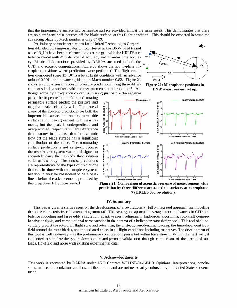
Preliminary acoustic predictions for a United Technologies Corpora-tion 4-bladed contemporary design rotor tested in the DNW wind tunnel(case 13_10) have been performed on a coarse grid with the HRLES tur-bulence model with 4th order spatial accuracy and 1st order time accura-cy. Elastic blade motions provided by DARPA are used in both theCFD, and acoustic computations. Figure 20 shows the two in-plane mi-crophone positions where predictions were performed. The flight condi-tion considered (case 13_10) is a level flight condition with an advanceratio of 0.3014 and advancing blade tip Mach number 0.82. Figure 21shows a comparison of acoustic pressure predictions using three differ-ent acoustic data surfaces with the measurements at microphone 7. Al-though some high frequency content is missing just before the negativepeak, the impermeable surface and rotatingpermeable surface predict the positive andnegative peaks relatively well. The generalshape of the acoustic predictions for both theimpermeable surface and rotating permeablesurface is in close agreement with measure-ments, but the peak is underpredicted andoverpredicted, respectively. This differencedemonstrates in this case that the transonicflow off the blade surface has a significantcontribution to the noise. The nonrotatingsurface prediction is not as good, becausethe overset grid system was not designed toaccurately carry the unsteady flow solutionso far off the body. These noise predictionsare representative of the types of predictionsthat can be done with the complete system,but should only be considered to be a base-line – before the advancements promised bythis project are fully incorporated.

IV. SummaryThis paper gives a status report on the development of a revolutionary, fully-integrated approach for modeling

the noise characteristics of maneuvering rotorcraft. This synergistic approach leverages recent advances in CFD tur-bulence modeling and large eddy simulation, adaptive mesh refinement, high-order algorithms, rotorcraft compre-hensive analysis, and computational aeroacoustics in the context of a helicopter rotor design tool. This tool shall ac-curately predict the rotorcraft flight state and rotor trim, the unsteady aerodynamic loading, the time-dependent flowfield around the rotor blades, and the radiated noise, in all flight conditions including maneuver. The development ofthis tool is well underway – as the preliminary computations presented within have shown. Within the next year, itis planned to complete the system development and perform valida tion through comparison of the predicted air-loads, flowfield and noise with existing experimental data.

V. AcknowledgmentsThis work is sponsored by DARPA under ARO Contract W911NF-04-1-0419. Opinions, interpretations, conclu-sions, and recommendations are those of the authors and are not necessarily endorsed by the United States Govern-ment.


Figure 20: Microphone positions inDNW measurement set up.

30º Deg.R

3R

Mic. 1

Mic 7 3R

Wind

Nondimensionalized Time

Tota

lAco

ustic

Pre

ssur

e(P

a)

0.2 0.4 0.6 0.8 1-30

-20

-10

0

10

20Measurement


Tota

lAco

ustic

Pre

ssur

e(P

a)

0 0.2 0.4 0.6 0.8 1-30

-20

-10

0

10

20Rotating Permeable Surface


Tota

lAco

ustic

Pre

ssur

e(P

a)

0 0.2 0.4 0.6 0.8 1-30

-20

-10

0

10

20Impermeable Surface


Tota

lAco

ustic

Pre

ssur

e(P

a)

0 0.2 0.4 0.6 0.8 1-30

-20

-10

0

10

20Non-rotating Permeable Surface

Figure 21: Comparison of acoustic pressure of measurement withprediction by three different acoustic data surfaces at microphone

7 (HRLES 3rd revolution).

The principal investigators who are listed as authors on this conference paper would like to acknowledge the skilledand enthusiastic efforts of the post-doctoral, graduate and undergraduate research assistants who have executed theefforts highlighted in this paper, in particular: Dr. Johannes N. Theron (Northern Arizona University) and Mr. BryanT. Flynt (Northern Arizona University, currently Stanford University), Dr. Roxana Vasilescu, Dr. Christopher Stone(currently Northern Arizona University), Dr. Yichaun Fang, Mr. Eric Lynch, Mr. Tim Eymann, Mr. Andrew Shel-ton, Mr. Kalen Braman, and Mr. Martin Sanchez-Rocha (Georgia Institute of Technology), Dr. Stephen Makinen,Mr. Matt Hill, Mr. Chris Hennes, and Mr. Seongkyu Lee (Pennsylvania State University).

We also extend our gratitude to Mr. Mark Potsdam and Dr. Roger C. Strawn (US Army Aeroflightdynamics Direc-torate), Dr. Tor Nygaard (Eloret Inc., Ames Research Center) for their assistance and access to the OVERFLOWcode, Dr. Casey Burley (NASA Langley) for providing supplemental descriptions regarding HART-I rotor parame-ters and experimental data, Dr. Joon Lim (NASA Ames) for his comments on the HART-I results and Dr. RalphNoack (ARL) for his assistance with integration of DiRTLib and SUGGAR.

We are particularly grateful to Dr. Lisa Porter of DARPA (now at NASA HQ) for initiating this project and for herprobing questions that helped improve our approach of the problem. Dr. Steve H. Walker is the current DARPAtechnical monitor and we are grateful for his continued encouragement.


VI. References

1 Jacobs, E. W., Mancini, J., Visintainer, J. A., and Jackson, T. A., “Acoustic flight test results for the Sikorsky S-76 QuietTail Rotor at reduced tip speed,” American Helicopter Society 53rd Annual Forum Proceedings, 1, 1997, pp. 23-41.

2 Edwards, B., Andrews, J., and Ranke, C., “Ducted tail rotor designs for rotorcraft and their low noise features,” Paper 18,AGARD Flight Integration Panel Symposium on Advances in Rotorcraft Technology, Ottawa, Ontario, Canada, May 27-30,1996.

3 Currier, J. M., Hardesty, M., O’Connell, J M., “NOTAR system - A quiet character,” American Helicopter Society andRoyal Aeronautical Society Technical Specialists’ Meeting on Rotorcraft Acoustics and Fluid Dynamics, Valley Forge, PA,Oct 1991.

4 Renaud, T., O'Brien, D. M., Smith, M. J., and Potsdam M., "Evaluation of Isolated Fuselage and Rotor-Fuselage Interac-tion using CFD," Presented at the American Helicopter Society 60th Annual Forum, Baltimore, MD, June 7-10, 2004.

5 Chan, W., Meakin, R., and Potsdam, M., "CHSSI Software for Geometrically Complex Unsteady Aerodynamic Applica-tions," AIAA Paper 2001-0593, AIAA 39th Aerospace Sciences Meeting and Exhibit, Reno, NV, January 2001.

6 Buning, P., "onsolidation of Time-Accurate, Moving Body Capabilities in OVERFLOW," http://www.arl.hpc.mil/Over - set2002, 6th Overset Composite Grid and Solution Technology Symposium, Fort Walton Beach, FL, October 2002.

7Jesperson, D., Pulliam, T., and Buning, P., "Recent Enhancements to OVERFLOW," AIAA Paper 1997-644, AIAA 35thAerospace Sciences Meeting and Exhibit, Reno, NV, January 1997.

8 Buning, P.G., Chiu, I.T., Obayashi, S., Rizk, Y.M. and Steger, J.L., “Numerical Simulation of the Integrated Space ShuttleVehicle in Ascent”, AIAA 88-4359, AIAA Atmospheric Flight Mechanics Meeting, Minneapolis, MN, Aug. 15-17, 1988.

9 Tor Nygaard personal communication, November 2004.

10 Spalart P.R. And Allmaras S.R, “A One-equation Turbulence Model for Aerodynamic Flows,” AIAA-92-0439, January1992.

11 Scott, N.W. and Duque, E.P.N. , “Using Detached Eddy Simulation and Overset Grids to Predict Flow Around a 6:1 Pro-late Spheroid”, AIAA Paper 2005-1362.

12 Menter, F.R. “Two-Equation Eddy-viscosity Turbulence Models for Engineering Applications”, AIAA Journal vol. 32 no8, 1994, pp 598-605.

13 Strelets M., “Detached Eddy Simulation of Massively Separated Flows”, AIAA-2001-0879, January 2001.

14 J.C. Kok, H.S. Dol, B. Oskam, H. van der Ven, “Extra-Large Eddy Simulation of Massively Separated Flows”, AIAA2004-264, January 2004.

15 Shelton, A., Abras, J., Hathaway, B., Sanchez-Rocha, M., Smith, M., and Menon, S., “An Investigation of the NumericalPrediction of Static and Dynamic Stall,” Proceedings of the 61st American Helicopter Society Annual Forum, Grapevine,TX, June 1-3, 2005.

16 Arunajatesan, S.; Kannepalli, C.; Dash, S.M., “Towards RANS-LES simulations of high speed shear flows”, Proceedingsof the ASME Fluids Engineering Division Summer Meeting, v 1, Proceedings of the 2001 ASME Fluids Engineering Divi-sion Summer Meeting. Volume 1: Forums, 2003, pp 15-21

American Institute of Aeronautics and Astronautics16

VI. References

17 Fang and Menon, “A Two-Equation Subgrid Model for Large-Eddy Simulation of High Reynolds Number Flows“,AIAA-2006-0116, January 2006

18 Yee, H.C., Sandham, N.D., Djomehri, M.J.,“Low Dissipative High Order Shock-Capturing Methods Using Characteristic-Based Filters,” Journal of Computational Physics, November1998.

19 Usta, E., “Application of a Symmetric Total Variation Diminishing Scheme to Aerodynamics of Rotors”, PhD Disserta-tion, Georgia Institute of Technology, August 2002.

20 Cho, Y. C., Boluriaan, S. and Morris, P. J., “Immersed boundary method for viscous flow around moving bodies,” AIAAPaper 2006-1089, 2006.

21 Mohd-Yusof, J., “Combined immersed-boundary-B-spline methods for simulations of flow in complex geometries,” CTRAnnual Research Briefs, NASA Ames Research Center/Stanford University, pp. 317-327, 1997.

22 Marshall, D., and Ruffin, S.M., " An Embedded Boundary Cartesian Grid Scheme for Viscous Flows using a New Vis-cous Wall Boundary Condition Treatment," AIAA Paper 2004-0581 Jan. 2004.

23 Noack, R., “SUGGAR: a General Capability for Moving Body Overset Grid Assembly”, AIAA 2005-5116, 17th AIAAComputational Fluid Dynamics Conference, June 6-9 2006, Toronto, Ontario, Canada

24 Noack, R., “DiRTlib: A Library to Add an Overset Capability toYour Flow Solver”, AIAA 2005-5116,17th AIAA Com-putational Fluid Dynamics Conference, June 6-9 2006, Toronto, Ontario, Canada

25 Nyaard, T.A., Saberi, H., Ormiston, R., Strawn, R.C. and Potsdam, M., “ Fluid Structure Interface for RotorcraftAeromechanic Computations”, personel communication, May 3, 2005.

26 Bauchau, O.A., Ahmad, J.U., “Advanced CFD and CSD Methods for Multidisciplinary Applications in Rotorcraft Prob-lems”, AIAA-96-4151-CP, Sixth AIAA/NASA/USAF Multidisciplinary Analysis and Optimization Symposium, pp. 1451-1451, Bellevue, WA, Sept.4-6, 1996.

27 Phanse, S., Sankar, L.N., and Bauchau, O.A., “An Efficient Tightly Coupled Fluid-Solid Interaction for Modeling Rotorsin Forward Flight.” Proceedings of the 2nd International Basic Research Conference on Rotorcraft Technology,Nanjing,China, Nov. 7-9, 2005

28 Bauchau, O.A., Bottasso, C.L. and Nikishkov, Y.G., “Modeling Rotorcraft Dynamics with Finite Element Multibody Pro-cedures”, Mathematical and Computer Modeling, Vol. 33, 2001, pp 1113-1137.

29 Tung, C., Caradonna, F.X., Boxwell, D.A., and Johnson, W.R., “Prediciton of Transonic Flows on Advancing Rotors,"40th Annual Forum Proceedings - American Helicopter Society, 1984, Arlington, VA, pp. 389-399

30 Potsdam, Mark, Yeo, Hyeonsoo and Johnson, Wayne, “Rotor airloads prediction using loose aerodynamic/structural cou-pling”, 60th Annual Forum Proceedings of the American Helicopter Society, Baltimore, MD, June 7-10, 2004, pp.497-518

31 Datta, Anubhav, Nixon, Mark, Chopra, Inderjit, “Review of Rotor Loads Prediction with the Emergence of RotorcraftCFD”, 31st European Rotorcraft Forum, Florence, Italy, September 13-15, 2005


VI. References

32 Brès, G.A., Brentner, K.S., Perez, G.*, and Jones, H.E., “Maneuvering Rotorcraft Noise Prediction,” Journal of Soundand Vibration, Vol. 39, No.3-5, August 2003, pp. 719–738

33Perez, G., Brentner, K.S., Brès ,G.A., and Jones, H.E.: A First Step Toward the Prediction of Rotorcraft Maneuver Noise.Journal of the American Helicopter Society, Vol. 50, No. 3, June 2005, pp. 230-237.

34Farassat, F. and Succi, G. P., “The Prediction of Helicopter Discrete Frequency Noise,” Vertica, Vol. 7, No. 4, 1983, pp.309-320.

35Ffowcs Williams, J. E. and Hawkings, D. L., “Sound Generation by Turbulence and Surface in Arbitrary Motion”, Philo-sophical Transactions of the Royal Society, London, Series A, Vol. 264, No 1151, May 1969, pp. 321-342.

36 R. A. Piziali, Ò2-D and 3-D Oscillating Wing Aerodynamics for a Range of Angles of Attack Including Stall,Ó NASATM 4532, USAATCOM TR 94-A-011, September1994.

37 Kufeld, R. M., D. L. Balough, et al. (1994). Flight testing the UH-60A airloads aircraft. Proceedings of the 50th AnnualForum. Part 1 (of 2), May 11-13 1994, Washington, DC, USA, American Helicopter Soc, Alexandria, VA, USA.

38 Lorber, P.F., Stauter, R.C., and Landgrebe, A.J.,"A Comprehensive Hover Test of the Airloads and Airflow of an Exten-sively Instrumented Model Helicopter Rotor," Proceedings of the 45th Annual, American Helicopter Society Forum,Boston, MA, May 1989.

39 Splettstoesser, W. R., R. Kube, Seelhorst, U., Wagner, W., Boutier, A., Michele, F., Mercker, E., Pengel, K. (1995).Higher Harmonic Control Aeroacoustic Rotor Test (HART) - Test Documentation and Representative Results. Braun-schweig, Germany, German Aerospace Research Establishment (DLR).

40 Yu, Y. H., Tung, C., van der Wall, B., Burley, C., Brooks, T., Beaumier, P.,Delrieux, Y., Mercker, E., and Pengel, K.,"The HART-II Test: Rotor Wakes and Aeroacoustics with Higher-Harmonic Pitch Control (HHC) Inputs – The Joint Ger-man/French/Dutch/US Project -," Proceedings of the 58th Annual Forum of the American Helicopter Society, Montreal,Canada, June 11-13, 2002.

41 Potsdam, M., Yeo, H. and Johnson, W.,"High Speed Forward Flight Rotor Airloads Prediction Using Loose Coupling,"Proceedings of the 60th Annual Forum of the American Helicopter Society, Baltimore, MD, June 7-10, 2004.


Documents

Revolutionary Physics-Based Design Tools for Quiet …personal.psu.edu/lnl/papers/AIAA-2006-1068.pdf · Revolutionary Physics-Based ... L.N. Sankar2, S. Menon3, O ... These aspects