Embed Size (px)
Citation preview

AIAA-2002-2839
REYNOLDS NUMBERS CONSIDERATIONS FOR SUPERSONIC FLIGHT
Brenda M. Kulfan Boeing Commercial Airplane Group
Seattle, Washington
32nd AIAA Fluid Dynamics Conference and Exhibit 24 - 26 Jun 2002 / St. Louis, Missouri
Page 1 American Institute of Aeronautics and Astronautics
Copyright 2002 by the American Institute of Aeronautics and Astronautics, Inc. All rights reserved.

Page 2 American Institute of Aeronautics and Astronautics
AIAA-2002-2838
REYNOLDS NUMBERS CONSIDERATIONS FOR SUPERSONIC FLIGHT Brenda M. Kulfan*
Boeing Commercial Airplane Group Seattle, Washington
ABSTRACT The viability of a High-Speed Civil Transport, HSCT, is very dependent on its cruise aerodynamic performance. The nature of the flow over a supersonic configuration changes through out its operating flight regime from low speed take off and landing condition, through subsonic cruise, transonic acceleration to supersonic cruise. The aerodynamic performance characteristics as well as the effectiveness of the control surfaces can be very dependent on both Reynolds Number and the flight Mach number. The lack of understanding Reynolds numbers effects, together with the inability to test at full scale conditions plus the uncertainties in the adequacy of CFD predictions lead to a number of fundamental Reynolds Number related questions:
• Are correct configuration decisions being made? • Are the correct high lift systems and control
surfaces being developed? • When is testing at low Reynolds adequate? • When is testing at high Reynolds number required? • Can CFD codes, validated with low Reynolds
number data, adequately predict forces, moments and flow characteristics at full-scale conditions?
• Do errors between experiment and theory imply of incorrect representation of the flow physics?
This paper will focus on the effects of Reynolds number on HSCT type configurations over the supersonic climb / cruise portions of the flight envelop. Many of the discussions and conclusions will apply equally to military type aircraft operation in a similar flight regime having similar geometric features. The general nature of possible types of surface flow, that a supersonic aircraft may encounter within its flight regime, will be summarized. Simplified flow analogies along with wind tunnel data and CFD computational results will be used to explore the dependency of the flow characteristics on specific geometric design features of an aircraft as well as upon Reynolds number. In the process, assessments will be made of the ability of the inviscid and Navier Stokes CFD methods to predict flow features, forces, moments and pressures at both wind tunnel and flight conditions. * Boeing Technical Fellow Aerodynamics
Mail stop 67-LF [email protected]
Copyright 2002 by the American Institute of Aeronautics, Inc. All rights reserved.
INTRODUCTION The viability of a High-Speed Civil Transport, HSCT, is very dependent on its cruise aerodynamic performance. The nature of the flow over a supersonic configuration changes through out its operating flight regime from low speed take off and landing condition, through subsonic cruise, transonic acceleration to supersonic cruise. Reynolds number and Mach number are the most familiar flow similarity parameter for aircraft applications. Two different scale models possess geometric similarity if the corresponding geometric dimensions of each model are all related by a single length scale factor. Matching the Reynolds number and the Mach number over two geometrically similar models will insure that the flows over each model will be dynamically similar in that the streamline patterns are geometrically similar, the general nature of the flows ( e.g. turbulent or laminar, attached or separated) will be identical and the dimensionless force coefficients are also the same. The performance characteristics of an HSCT, as well as the effectiveness of the control surfaces may be very dependent on Reynolds Number as well as on the flight Mach number. The Reynolds number consequently is the primary aerodynamic scaling parameter used to relate sub-scale wind tunnel model experiments to full scale airplanes in flight. A number of recent investigations have focused on the effects of Reynolds number on HSCT type configurations in the subsonic high lift conditions1, transonic cruise / climb conditions 2 as well as on the stability and control characteristics 3 over the same flight regimes. Similar investigations have been made for fighter type configurations 4, 5. This paper will focus on the effects of Reynolds number on HSCT type configurations over the supersonic climb / cruise portions of the flight envelop. Many of the discussions and conclusions will apply equally to military type aircraft operation in a similar flight regime having similar geometric features. Specific design features and aerodynamic characteristics, which may be significantly influenced by Reynolds number, will be discussed. Current wind tunnels Reynolds number testing capabilities will be reviewed. It will be shown that the existing testing limitations lead to a number of fundamental questions and concerns relative to the design, performance and viability of a High Speed Civil Transport, HSCT. The general nature of possible types of surface flow, that a supersonic aircraft may encounter within its flight regime, will be summarized. Simplified flow analogies along with wind tunnel data and CFD computational

Page 3 American Institute of Aeronautics and Astronautics
results will be used to explore the dependency of the flow characteristics on specific geometric design features of an aircraft as well as upon Reynolds number. Specific Reynolds number effects will be explored in three general areas:
• Attached flow conditions typically associated with the cruise conditions
• Shock / boundary layer interactions at near cruise conditions
• Leading edge vortex flow at off design conditions
In the process, assessments will be made of the ability of the inviscid and Navier Stokes CFD methods to predict flow features, forces, moments and pressures at both wind tunnel and flight conditions. We will also attempt to answer the intriguing questions:
• Will the difference between a low Reynolds number viscous CFD calculation and a corresponding inviscid CFD calculation always “Bracket” the flow characteristics at full scale conditions?
• Is shock induced boundary layer separation strongly influenced by Reynolds number?
• Does Reynolds affect the movement of the origin of a leading edge vortex on a swept wing with a round leading edge?
It will be shown that coordinated wind tunnel test programs and extensive code validation studies will be necessary to properly predict and understand full scale conditions.
REYNOLDS NUMBER CONSIDERATIONS A high speed civil transport is a highly integrated slender design that operates over a wide flight regime that includes:
• High lift takeoff and landing conditions • Subsonic climb and cruise • Transonic and supersonic acceleration • Supersonic cruise
Geometric variations such as flap deflection are utilized to create additional lift or to optimize the aerodynamic performance along the flight path. The geometrical variations along with the wide range operating Mach numbers, lead to many areas of design as well as performance and control that may be significantly affected by Reynolds Number as shown in figure 1. Wind tunnel testing of small scale models is a vital element in the design, evaluation and performance data base generation of any new aircraft configuration. The operating Reynolds number capabilities of various wind tunnels facilities are compared in figure 2 along with the Reynolds numbers range corresponding to a
nominal mission profile for a typical HSCT configuration1. This leads to the wind testing dilemma associated with HSCT configuration development. As shown in the figure, it is not possible to conduct wind tunnel testing at full scale Reynolds numbers for the supersonic cruise design condition, nor for important flight conditions corresponding to high lift operation, and transonic / supersonic climb. Three options are generally available to generate aerodynamic data at the flight Reynolds numbers:
1. Simple flat plate skin friction theory is used to extrapolate the wind tunnel data to full scale conditions. This is typically the approach used to generate the extensive performance database required for the development of a commercial aircraft configuration.
2. Calibrated CFD methods are used to calculate the aerodynamic data for both the wind tunnel model and the full scale airplane. The theoretical increments between the two sets of data are applied to the wind tunnel database to obtain either the full scale performance, or to obtain an adjusted database which is then extrapolated to full scale conditions using the flat plate skin friction theory.
3. Use the wind tunnel to evaluate and calibrate the CFD methods. The CFD methods are then used to predict the performance and flow characteristics at full scale conditions. This is the typical approach used for aerodynamic evaluations during the design development process.
There are a number of assumptions inherent in each of these options. The key assumption of the first option is that the fundamental flow physics on the wind tunnel model are unaffected by the Reynolds number differences between the model at test conditions and the airplane at flight conditions. It is therefore also assumed that the pressure related forces and moments are essentially the same on the model and the airplane. Therefore the only difference in aerodynamic forces between the airplane and the wind tunnel model is in the viscous drag force. The final assumption is that the viscous drag difference can be determined as the increment between simple flat plate theory skin friction predictions on the airplane and on the wind tunnel model at the corresponding Mach numbers. The fundamental assumption of the second option is that CFD methods can capture correctly the differences in nature of flow physics on the airplane and on the wind tunnel model and therefore and can also adequately predict the associated changes in the viscous and pressure forces and moments. The adjusted wind tunnel data is then extended to full scale conditions

Page 4 American Institute of Aeronautics and Astronautics
either as in option 1 or by CFD calculations on the airplane at the flight conditions. The third options precludes the use of wind tunnel data and assumes that the CFD predictions can adequately predict the flow physics and associated forces and moments on the airplane at flight conditions. This is often used to check the aerodynamic performance of the airplane at a limited number of flight conditions during the aerodynamic design process. With any of these options adjustments must be made to account for differences between the wind tunnel model geometry and the airplane, and to include additional drag adjustments to account for excrescence drag, power effect related drag items and other miscellaneous drag items. Coordinated CFD and wind tunnel validation studies are very necessary to establish the validity and the consistency of the CFD predictions. The wind tunnel testing Reynolds number limitation dilemma is further complicated by aeroelastic distortion effects on wind tunnel model geometry that is associated with variations in either Mach number or dynamic pressure as shown by the example in figure 3. The effect of Reynolds number on wing twist is really a dynamic pressure effect since in conventional wind tunnels, Reynolds numbers variations are accompanied by changes in the dynamic pressure. The wing twist variation is nearly a linear variation of the free stream dynamic pressure. The aeroelastic effect of increasing Mach number at a fixed Reynolds number is caused by the reduction in lift as Mach number is increased. These aeroelastic distortions can be minimized when testing in the NTF by conducting, where possible, Reynolds number variations at a fixed dynamic pressure. Typically, wing washout caused by the model aeroelastics is evident in both the lift and pitching moment curves. The drag polars often appear to be quite insensitive to the aeroelastic distortions since both the drag and lift are decreased by increased wing washout. In any case, it is important to account for the aeroelastic distortions in the final analysis of the wind tunnel data, particularly if the test data is to be used for CFD code validation studies. Aerodynamic cruise drag has a highly leveraged effect on the size and performance of an HSCT design. As shown in figure 4, a design improvement that results in a reduction of supersonic drag of 1% , which is approximately 1 drag count, (∆CD ~ 0.0001), will result in a reduction of approximately 10,400 lb. in the design Maximum Takeoff Gross Weight, MTOW. This also results in a fuel saving of about 7,500 lb. The net benefits are equivalent to reduction in the structural weight of more then one ton.
A reduction of one count of drag for the subsonic climb / cruise portion of the HSCT mission profile will reduce the design gross weight by about 1500 lb. A reduction of one drag count over the transonic / low-supersonic portion of the flight profile results in a design gross weight reduction of more then 1000 lbs. In addition, an unexpected increase in supersonic drag for a specific HSCT design would result in a 50 mile loss in range capability and thus could be a significant consideration in meeting the design objectives and performance guarantees. Relatively small changes in drag can therefore greatly impact the design selection and definition of the features of an optimized supersonic configuration, as well as determining its ultimate performance capabilities. This fact further emphasizes the need to understand and to properly account for the effects of the Reynolds number differences between a wind tunnel database and the full scale flight conditions. The inability to test at full scale conditions plus the uncertainties in the adequacy of CFD predictions, result in a number of fundamental Reynolds Number questions related to the design and aerodynamic assessment of a HSCT:
• Can we predict the flight performance, stability levels and control effectiveness?
• Can we make correct configuration design decisions?
• Are the right high lift systems and control surfaces being developed?
• When is testing at low Reynolds adequate? • When is testing at high Reynolds number
required? • Can CFD codes, validated with low Reynolds
number data, adequately predict forces, moments and flow characteristics at full-scale conditions?
• Will the final design meet the design criteria and performance guarantees?
Typically, the full scale database for a new configuration concept is developed from an extensive wind tunnel database obtained from a variety of scale models. The full scale database is then developed by applying adjustments to the wind tunnel database that account for differences in geometry between the model and the airplane, accounting for power and trim effects, scaling the viscous drag to full scale conditions and applying appropriate miscellaneous drag corrections such as protuberance and excrescence drag. It is this drag level upon which initial airplanes are sold and guarantees are made. When the initial configurations are flown, a flight test data base is then obtained to correlate with the pre-
Page 5 American Institute of Aeronautics and Astronautics
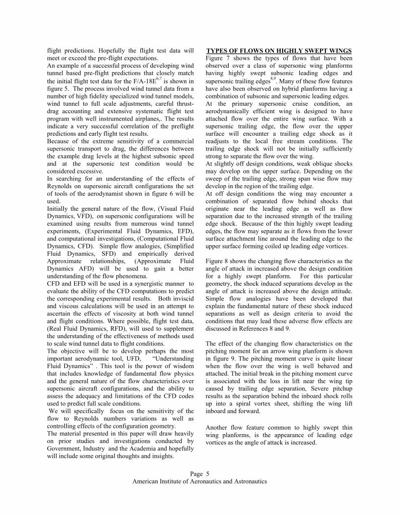
flight predictions. Hopefully the flight test data will meet or exceed the pre-flight expectations. An example of a successful process of developing wind tunnel based pre-flight predictions that closely match the initial flight test data for the F/A-18E6,7 is shown in figure 5. The process involved wind tunnel data from a number of high fidelity specialized wind tunnel models, wind tunnel to full scale adjustments, careful thrust- drag accounting and extensive systematic flight test program with well instrumented airplanes,. The results indicate a very successful correlation of the preflight predictions and early flight test results. Because of the extreme sensitivity of a commercial supersonic transport to drag, the differences between the example drag levels at the highest subsonic speed and at the supersonic test condition would be considered excessive. In searching for an understanding of the effects of Reynolds on supersonic aircraft configurations the set of tools of the aerodynamist shown in figure 6 will be used. Initially the general nature of the flow, (Visual Fluid Dynamics, VFD), on supersonic configurations will be examined using results from numerous wind tunnel experiments, (Experimental Fluid Dynamics, EFD), and computational investigations, (Computational Fluid Dynamics, CFD). Simple flow analogies, (Simplified Fluid Dynamics, SFD) and empirically derived Approximate relationships, (Approximate Fluid Dynamics AFD) will be used to gain a better understanding of the flow phenomena. CFD and EFD will be used in a synergistic manner to evaluate the ability of the CFD computations to predict the corresponding experimental results. Both inviscid and viscous calculations will be used in an attempt to ascertain the effects of viscosity at both wind tunnel and flight conditions. Where possible, flight test data, (Real Fluid Dynamics, RFD), will used to supplement the understanding of the effectiveness of methods used to scale wind tunnel data to flight conditions. The objective will be to develop perhaps the most important aerodynamic tool, UFD, “Understanding Fluid Dynamics” . This tool is the power of wisdom that includes knowledge of fundamental flow physics and the general nature of the flow characteristics over supersonic aircraft configurations, and the ability to assess the adequacy and limitations of the CFD codes used to predict full scale conditions. We will specifically focus on the sensitivity of the flow to Reynolds numbers variations as well as controlling effects of the configuration geometry. The material presented in this paper will draw heavily on prior studies and investigations conducted by Government, Industry and the Academia and hopefully will include some original thoughts and insights.
TYPES OF FLOWS ON HIGHLY SWEPT WINGS Figure 7 shows the types of flows that have been observed over a class of supersonic wing planforms having highly swept subsonic leading edges and supersonic trailing edges8,9. Many of these flow features have also been observed on hybrid planforms having a combination of subsonic and supersonic leading edges. At the primary supersonic cruise condition, an aerodynamically efficient wing is designed to have attached flow over the entire wing surface. With a supersonic trailing edge, the flow over the upper surface will encounter a trailing edge shock as it readjusts to the local free stream conditions. The trailing edge shock will not be initially sufficiently strong to separate the flow over the wing. At slightly off design conditions, weak oblique shocks may develop on the upper surface. Depending on the sweep of the trailing edge, strong span wise flow may develop in the region of the trailing edge. At off design conditions the wing may encounter a combination of separated flow behind shocks that originate near the leading edge as well as flow separation due to the increased strength of the trailing edge shock. Because of the thin highly swept leading edges, the flow may separate as it flows from the lower surface attachment line around the leading edge to the upper surface forming coiled up leading edge vortices. Figure 8 shows the changing flow characteristics as the angle of attack in increased above the design condition for a highly swept planform. For this particular geometry, the shock induced separations develop as the angle of attack is increased above the design attitude. Simple flow analogies have been developed that explain the fundamental nature of these shock induced separations as well as design criteria to avoid the conditions that may lead these adverse flow effects are discussed in References 8 and 9. The effect of the changing flow characteristics on the pitching moment for an arrow wing planform is shown in figure 9. The pitching moment curve is quite linear when the flow over the wing is well behaved and attached. The initial break in the pitching moment curve is associated with the loss in lift near the wing tip caused by trailing edge separation, Severe pitchup results as the separation behind the inboard shock rolls up into a spiral vortex sheet, shifting the wing lift inboard and forward. Another flow feature common to highly swept thin wing planforms, is the appearance of leading edge vortices as the angle of attack is increased.

Page 6 American Institute of Aeronautics and Astronautics
By virtue of extensive experimental and semi-empirical investigations 10 to 16, the formation of the leading edge separation vortex is well understood. On a supersonic wing, the leading edge vortex can develop providing that the component of Mach number normal to the leading is subsonic. Experimental investigations have established the boundary shown figure 10 that divides the regions for attached flow and for leading edge separated flow for flat wings with thin sharp leading edges. The separation boundary is defined in terms of the Mach number normal to the leading edge, MN, and the angle of attack normal to the leading edge αN, in degrees, by the expression:
MN = 0.6 + 0.013 αN MN and αN are defined in terms of the free stream Mach number, angle of attack and leading edge sweep in the figure. The separation boundary equation has been used to construct the chart in the lower right side of the figure that shows the variation of the separation boundary with leading edge sweep for a wing with a straight leading edge. The results of extensive wind tunnel investigations of the nature of the flow over flat swept wings with thin sharp leading edge expanded the identification of boundaries between the various classes of flows17 as shown in Figure 11. For wing planforms in which the leading edge is swept behind the free stream Mach line, the use of wing camber along with round leading edge airfoils can result in a region of attached flow at low angles of attack , and to shift the other boundaries to higher angles of attack. However, similar classes of flows such as shown in figure 11 may ultimately be expected to also exist on these wing designs. As shown in figure 12, supersonic aircraft configurations may encompass a wide variety design features. The features of each design will ultimately determine the unique nature of the flow characteristics over its operating envelop. However, for each configuration, the three classes of flows may be expected to ultimately develop somewhere within its flight envelop. These include conditions that are primarily dominated by:
1. attached flow 2. shock / boundary layer induced separations 3. leading edge vortex flows
The paper will focus on identifying the effects of Reynolds number differences between typical wind tunnel test conditions and full scale conditions on these three general classes of flows in the above order. The format of the paper will therefore, be composed of three major sections corresponding to the three general classes of flows.
PART 1: REYNOLDS NUMBER EFFECTS FOR ATTACHED FLOW CONDITIONS
The evolution of the current supersonic aerodynamic design capability from a linear theory point design process to the current non-linear multi-point design process will be discussed. Comparisons will be made between predicted aerodynamic performance data and corresponding wind tunnel test data for designs that were developed by the classic linear theory design process, by a refined linear theory design process and by a current non-linear design process. The discussions will separate the aerodynamic drag into the pressure drag which relates to the aerodynamic design and the achieved flow characteristics, and the viscous drag which typically has the greatest variation with Reynolds number. We will focus on answering the following questions:
• How good are the CFD predictions of pressures, forces and moments at wind tunnel conditions?
• What is the expected effect of increases in Reynolds numbers on pressure drag, viscous drag, lift and pitching moments?
• Does a comparison of inviscid and viscous code pressure drag predictions at wind tunnel conditions results “bracket” full scale pressure drag levels?
• How good are the methods used to scale the viscous drag to full scale conditions?
Excrescence drag considerations and the effect of Reynolds number increases on boundary layer growth will also be discussed. The classic linear theory supersonic design process is shown conceptually in figure 13. The fundamental approach is to conduct linear theory design optimization and design integration to minimize the drag at the cruise condition. Calculated pressure distributions are compared with a set of real flow limiting design criteria8,9. If the limiting design criteria, the design is iterated and rechecked again. A wind tunnel model is built and tested to validate the anticipated performance levels. Leading edge and trailing edge flaps are deflected to minimize the drag at the low supersonic, transonic and subsonic off design conditions. The full scale airplane data base is then developed from the wind tunnel data base by accounting for any geometric differences between the model and the airplane, adding in estimates of excrescence and miscellaneous drag and power effects, and using flat plate skin friction theory to account for the difference in viscous drag at flight and wind tunnel conditions. Early US SST development studies as shown in figure 14 have confirmed that linear theory aerodynamic designs that satisfy the set of the previously mentioned

Page 7 American Institute of Aeronautics and Astronautics
real flow design criteria, appear to achieve in the wind tunnel, the theoretical inviscid drag levels including calculated turbulent skin friction drag. The designs developed by linear theory designs are heavily constrained by the real flow constraints and are therefore considered to be on the conservative side in terms of the aerodynamic performance. Hence it is not surprising that the inviscid predictions of drag match the wind tunnel test data. For this designs, the pressure drag should not vary significantly between wind tunnel and full scale flight condition. The major uncertainty is perhaps the ability to scale the viscous forces to the flight conditions using flat plate skin friction theory. This will be discussed in greater detail further on in the paper A refined linear design process developed early in the initial HSCT studies is shown in figure 15. This process differs from the classic linear theory design process in the following areas:
• Wing leading edge design considerations 10,11 based controlling the formation of leading edge vortices at off design conditions are included in the wing airfoil definitions.
• Non-linear CFD inviscid and / or viscous analyses are made of the linear design to establish the expected performance levels and to insure the success of achieving the performance levels.
• The non-linear CFD codes can also be used to parametrically optimize the off design flap deflections.
• The viscous drag differences between wind tunnel and flight could be determined either using either flat plate skin friction theory or Navier-Stokes calculations.
Since the design optimization element in the design process is still based on linear theory, the resulting aerodynamic designs are also considered to be mildly conservative. Once again, it is expected that the inviscid and viscous drag estimates of the pressure drag should be nearly identical for successful designs and would not be expected to vary significantly with Reynolds number. Figures 16, 17 and 18 show the results of a code validation efforts18,19 undertaken at Boeing to understand the capabilities of advanced viscous and inviscid computational fluid dynamic codes to predict the flow about HSCT type configurations. The wind tunnel model was a 1.7% scale model that was tested in the Boeing supersonic wind tunnel. This configuration was designed using the previously described modified linear theory design process. Figure 16 contains comparisons of the experimental pressure distributions with the corresponding viscous and inviscid predictions obtained using a parabolized Navier-Stokes code.
Both the inviscid and viscous predictions show very good agreement with the experimental pressure distributions levels and shapes especially in what is considered region near the leading edge. The inviscid and viscous CFD predictions are very similar except where the inviscid solution appears to have over predicted the severity of the upper surface cross-flow shock that is particularly evident at 2 degrees above the design angle of attack. Colored oil flow runs were made during the wind tunnel experiments to examine the nature of the flow on the wing upper surface, in particular near the cruise point at Mach 2.4. Inviscid and viscous particle traces were calculated near the surface at the same Mach number and lift coefficient. The computed particle traces are compared with the experimental oil flow in figure 17. The viscous flow calculated particle trace matches the details oil flow surface patterns quite well. The inviscid particle trace matches the overall flow characteristics but does not capture the viscous related detailed features that include:
• inboard flow turning near the wing leading edge / body intersection region
• flow turning across the mild inboard flow related forward swept shock
• body off-flow onto the wing near the wing body junction area
Force calculations obtained with the inviscid and viscous CFD analyses19 and with linear theory, are compared with wind tunnel test data at Mach 2.4 in figure 18. The inviscid codes included the TRANAIR full potential code, and a parabolized Euler code. The viscous analyses were obtained with a parabolized Navier-Stokes code. Flat plate skin friction drag estimates were added to the inviscid CFD drag calculations, and to the linear theory predictions to obtain the total aerodynamic drag. The viscous and inviscid force and moment predictions all agree quite well with the test data. The linear theory drag predictions depart from the test data at the higher CL above the design condition. Linear theory over estimated the lift and shows a large difference in the pitching moment predictions and the test data. The differences in the flow field characteristics and in the pressure distributions shown in the previous pictures apparently did not result in measurable differences in either the forces or moments. Since the CFD viscous and inviscid force, moment and pressure data are nearly identical it is expected that the full scale pressure , lift and moment data for the wing / body configuration would be unaffected by the Reynolds number differences.

Page 8 American Institute of Aeronautics and Astronautics
Figures 19 and 20 contain comparisons of inviscid drag predictions obtained using the AIRPLANE Euler code with wind tunnel test data for the Boeing Ref H wing/body/nacelle configuration. This configuration was also developed by the refined linear theory design process. The inviscid CFD predictions are once again seen to closely match the low Reynolds number wind tunnel test data for this class of designs. This again implies that viscosity does not greatly affect the flow physics near the design condition, and that the flow physics would be similar at the full scale flight condition. The viscous drag would have to be adjusted for the differences in the test and flight Reynolds numbers Figure 21 contains a comparison of inviscid and viscous predictions of the wing pressure distribution obtained using CFL3D, with the corresponding wind tunnel test data. The theoretical pressure distributions are nearly identical except in a small region on the wing upper surface. The viscous pressure distribution predictions are in excellent agreement with the test data. Navier Stokes predictions of the pressure drag on the Ref H wing/body at zero lift and near the cruise CL are shown in figure 22 for both wind tunnel and full scale Reynolds numbers. Euler Predictions are also shown. These predictions were made at the design Mach number of 2.4. The full scale pressure drag is approximately one drag count lower then the corresponding wind tunnel drag levels at the cruise CL and Mach number. The full scale drag levels are approximately three tenths of a drag count less then the wind tunnel levels near zero lift. The effect of the Reynolds number increase is seen to be actually slightly beneficial and is likely associated with a reduction in the boundary layer displacement thickness at the larger Reynolds numbers. The full scale predictions are seen to fall between the wind tunnel predictions and the Euler predictions. The current non-linear supersonic aerodynamic design process20,21 is shown in figure 23. The non-linear element of the design process starts from an initial “seed” geometry developed by the refined linear theory design approach. Currently the non-linear design optimization utilizes either Euler or non-linear full potential CFD codes. This process enables a large number of geometry constraints to be imposed. The optimization process may include either single point cruise optimization with supplementary off-design flap deflection optimization or direct multi-design point optimization. After a complete converged inviscid design cycle has been completed, the resulting geometry is then typically analyzed with a Navier-Stokes code for the performance evaluation.
The results of three independent non-linear optimization studies starting from the same initial “seed” geometry are shown in figure 24. The inviscid and viscous predictions of each optimized design are shown as drag improvements to the baseline geometry. Substantial cruise drag reductions were achieved by each design. It appears that the greater the drag improvement, the larger is the difference between the viscous and inviscid drag predictions. This seems to imply that the non-linear designs are more aggressive then the conservative linear theory methods and that at increased Reynolds numbers the drag improvement would approach the levels suggested by the inviscid levels. Based on the sensitivities shown in figure 4, the gross weight of the sized airplane would be between 12,000 to 21,000 lbs lighter if the inviscid drag levels were indeed achieved at the flight conditions. The previous discussions have focused primarily on pressure related forces and moments. In figure 25, comparisons are made of predictions of both pressure drag and viscous drag for the 2.2 % Ref H wind tunnel model for a range of Reynolds numbers. Again it is seen that for this particular design, increasing Reynolds had a very slight effect on the predicted pressure drags. The CFD viscous drag calculations are compared with flat plate skin friction drag estimates and with the viscous drag deduced from the wind tunnel measurements by subtracting the theoretical pressure drag. It is seen that Reynolds number has a large effect on the viscous drag and also that the viscous drag estimates by the three methods differ significantly.
VISCOUS DRAG PREDICTION During Recent HSCT studies significant variations were observed in viscous drag predictions that were obtained by different organizations using different CFD codes and a variety of models, as shown in figure 26, There were substantial differences in flat plate theory predictions and also between the viscous CFD predictions. This posed a concern since each organization was developing optimized configurations using their favored CFD tools. If the tools produced different answers on a common analysis configuration, how valid would comparisons be of different design options predicted by the different codes? Similar differences between viscous drag predictions22 obtained using different turbulence models, are shown in figure 27. This figure contains a comparison of an experimental wind tunnel model drag polar with CFD drag predictions using four different turbulence models. The differences between the theoretical predictions and

Page 9 American Institute of Aeronautics and Astronautics
the measured drag level at an angle of attack of 5 degrees are also shown. The theoretical predictions were all substantially less then the test data. Theory under predicted the measured drag by 8 to 15 drag counts ( -0.0008 to –0.0015). Comparisons were made of the CFD viscous drag predictions of the for the model with drag estimates made using flat plate theory. The differences between the CFD predictions of the viscous drag and the flat plate viscous drag were found to be very similar to the test versus theory differences shown in figure 27. The CFD viscous predictions varied from 12.5% to 28.1% lower then the flat plate predictions. The drag polar predictions with the CFD viscous drag predictions replaced by the flat plat theory nearly match the test data as shown in the Figure 28. There appears, therefore, a substantial and inconsistent error in CFD viscous drag predictions. It is felt that an important element, in validating the viscous drag predictions of any Navier Stokes code, is to make sure that predictions of the local and average skin friction drag and boundary layer characteristics must match the “simple” flat plate measured skin friction test data over the range of Mach numbers and Reynolds for which the codes will be used. Consequently a study was conducted as part of the HSCT program to assess the ability of the CFD codes to predict the skin friction drag on a flat plate for fully turbulent flow conditions. The first phase23, involved the formulation of an experimental database of fully turbulent flow skin friction measurements on flat plate adiabatic surfaces at subsonic through supersonic Mach numbers and for a wide range of Reynolds numbers. Statistical analyses of the data were conducted to establish appropriate skin friction equations to represent the database for use in evaluating the viscous drag predictions by various Navier Stokes codes. Improved flat plate skin friction prediction equations that matched the mean of the skin friction database values were developed in the process. In the second phase24, CFD flat plate viscous drag predictions were made using a number of different Navier-Stokes codes, various turbulence models and different participating organizations. These included Boeing Phantom Works, Long Beach, (BPW-LB); NASA Ames Research Center, (ARC) and Boeing Commercial Airplane Group in Seattle, (BCAG).
TURBULENT FLOW SKIN FRICTION In Phase 1, flat plate skin friction data were obtained from a number of experimental sources. These data cover a wide range of Mach numbers and Reynolds numbers. Comparisons were made with various flat plate theories to select the theory that most closely matched the test data. The results of these assessments
are presented in the Reference 23 and are summarized in figure 29. The flat plate theory is based on the reference temperature method. This method assumes that the incompressible skin friction equations apply to supersonic Mach numbers provided that the density and viscosity are calculate at some reference temperature that represents the variation of temperature across the boundary layer. The left figure shows the comparison of the modified Shultz / Grunow equation with incompressible test data. Statistical analysis of the differences between the test data and corresponding Cf predictions shows that the mean of the differences is ∆Cf = -.000000671 which corresponds to an average difference of 0.13% .The standard deviation of data about the mean is approximately 0.7 counts of drag ( ∆Cf = 0.000067) which corresponds to 2.8% of the corresponding predicted value. The modified Shultz / Grunow equation therefore appears to provide an accurate estimate of incompressible local skin friction coefficient over the entire range of Reynolds Numbers covered by the test data. The figure on the right shows transformed experimental skin friction data for six different sets of test data obtained at Mach numbers from 1.7 to 2.95. The Kulfan T* equation23, was used for the transformation process. The “mean” of the differences between the transformed skin friction data and the incompressible Cf predictions is essentially zero. The “ scatter” of the test has a standard deviation of about 1 drag count ( ∆Cf ~ 0.0001). This corresponds to about a 3.8% scatter of the test data about the theoretical Cf predictions over the entire Reynolds number range and Mach number conditions represented by the test data. The “scatter” in the compressible theoretical - experimental transformed skin friction increments are only slightly higher than the scatter in the incompressible data. ( 0.7 counts versus 1 count). The CFD codes used included the CFL3D code and the OVERFLOW code. The turbulence models used in the calculations were representative of turbulence model categories22,25 ranging from most simple to most sophisticated and include:
• “zero-equation” (algebraic) model - Baldwin- Lomax26,27
• “one-equation” model - Spalart- Allmaras28 • “two-equation” model - Menter’s SST29,30
Typical phase 1 results are shown in figure 30. In this figure local skin friction calculated with the Spalart-Allmaras turbulence model using the OVERFLOW code are compared with the flat plate theory.

Page 10 American Institute of Aeronautics and Astronautics
At Mach 0.9, the CFD predictions vary from - 2 % to +1% of the flat plate theory over the wind tunnel to flight Reynolds number range. At Mach 2.4, the CFD predictions are from 4% to 5.5% higher then the flat plate predictions. Figure 31 contains a comparative summary of all of the CFD average skin friction predictions made in the study, relative to the flat plate theory and hence to the mean of the experimental flat plate. The comparisons shown are for Mach 0.5 or 0.9 and Mach 2.4 or 2.5. The scatter band for the test data relative to the flat plate theory is also shown in the figure. It is seen that the variations in the CFD predictions greatly exceeds the scatter of the test data. Viscous drag predictions for a full scale aircraft are typically obtained either by extrapolation of wind tunnel results to full-scale conditions, or by prediction of the drag of an airplane at full-scale conditions. In order to understand the potential impact of the uncertainties in the viscous drag predictions, the differences between the CFD predictions and the flat plate theory have been converted into airplane drag counts. The equivalent drag counts are obtained by multiplying the average skin friction increments by the wetted area ratio, Awet/Sref, for a typical HSCT type configuration of approximately 3.5. The impacts of the uncertainty of the viscous drag prediction differences on the prediction of the full scale drag using the aforementioned two approaches, are shown in figure 32 and 33. In order to understand the potential impact of the uncertainties in the viscous drag predictions, the differences between the CFD predictions and the flat plate theory have been converted into airplane drag counts. The equivalent drag counts are obtained by multiplying the viscous drag increments by the ratio of the wetted area to the wing reference area. This ratio is about 3.5 for a typical HSCT type configuration: At the subsonic condition, the average error of all the full scale predictions, shown in figure 32, is about 1 drag count low and the range of errors varies from – 2.6 to +1.5 drag counts. The average error at Mach 2.4 is +1.66 drag counts high, with a range of errors from –0.7 to +3.1 drag counts. This differences in the friction drag predictions at full scale Reynolds numbers of ∆CD ~ 0.00038 is equivalent to an uncertainty in the design MTOW of nearly 40,000 lbs or would result in a range difference of 190 nmi. Figure 33 shows the results of using the various CFD methods to determine the difference in viscous drag at wind tunnel and full scale conditions relative to the corresponding increment determined from flat plate theory.
In this instance, nearly all of the CFD methods would predict higher drag levels for the airplane relative to extrapolation of a wind tunnel database to full scale using flat plate skin friction. Figure 34 shows the results of an extensive study31 of predictions of compressible skin friction over a wide range of Reynolds Numbers and Mach numbers. The predictions were made using the Navier-Stokes method PAB3D with two different algebraic Reynolds stress turbulence models. The CFD predictions were converted in equivalent incompressible skin friction values using the Sommer-Short “T*” method and compared with the Karmen- Schoenherr incompressible skin friction values for fully turbulent and partly laminar flow. The results Indicated that at the lower Reynolds numbers 3 to 30 million, Both the Turbulence models predicted the skin-friction coefficients within 2 % of the semi-empirical results. At the higher Reynolds Numbers corresponding to full scale conditions, the results obtained using the Girimaji turbulence model over predicted the semi-empirical results by 10% while the results using the turbulence model by Shih, Zhu, and Lumley under predicted the flat plate theory by 6 %. Available flight test measurements of skin friction have also been analyzed to help assess the uncertainty of skin friction drag at supersonic speeds. As part of the HSR program, co-operative flight test experiments between Boeing, NASA and Tupolev were conducted using a modified TU-144LL supersonic airplane. One of the test experiments included skin friction and boundary layer measurements as indicated in Figure 35. Preliminary local skin friction from the TU-144LL flight experiments are compared with the flat plate local skin friction method of Reference 23 in figure 36. The initial study results indicate an uncertainty in the local skin friction predictions of +/- 2 % to +/- 4 %. The results of flight test measurements of local skin friction on the Concorde32 are shown in Figure 37. Six measuring blocks were installed on the airplane. Each one consisted of two Preston tubes, one static probe and one thermal couple to measure the wall temperature. The data obtained with the smaller Preston tube and expressed as equivalent incompressible skin friction coefficients, are compared with the empirical incompressible skin friction formulations of Michel and the Schultz-Grunow. The maximum variation between the measured skin friction and the Michel Relation is on the order of 25%. The flight test data appear to agree slightly better with the Schultz-Grunow incompressible skin friction equation

Page 11 American Institute of Aeronautics and Astronautics
Comparisons were also made with skin friction predictions obtained with a three dimensional boundary layer code using pressure distributions obtained by an Euler code. The results in Figure 38 indicate that the differences between the boundary layer calculations and the test data are smaller then the differences between the test data and the Michel flat plate skin friction theory. However the differences in the predictions and the test data are still significant and are on the order of +/- 10%. Flight test skin friction measurements have also been obtained on the YF-12A airplane33. Figure 39 shows the results of these in-flight measurements. The local skin friction drag have been transformed into equivalent skin friction values and are compared with flat plate theory. The skin frictions measurements are presented in terms of Reynolds numbers based on the distance from the nose of the aircraft. Skin friction measurements were taken at the five stations shown in the figure. Pressure measurements that were taken along the bottom on the airplane where the skin friction data was obtained showed that the pressure coefficients were positive and were quite a bit above zero. Past studies have indicated that local skin friction measurements in regions of positive pressure coefficients results in lower skin friction coefficients. At stations 1 and 4 the measure pressure coefficients were nearly zero. Consequently only the data obtained from those two stations are shown in figure 39. The flight test data are seen to vary significantly from the corresponding flat plate theoretical skin friction theory. Both the flight test data and the skin friction theory trends with Reynolds number are, however, quite similar. These results along with the previously comparisons of test data, semi-empirical skin friction predictions, CFD viscous drag predictions and flight test measurements show that the scaling of viscous drag to full scale skin friction drag remains an area of significant uncertainty. In the process of developing flight data for an airplane from a wind tunnel database, the excrescence drag associated with the fabrication and manufacturing surface irregularities, must be accounted for. The excrescence drag for a supersonic transport is typically on the order of 5 to 8% of the skin friction drag. Excrescence drag predictions currently rely heavily on the use of experimental databases of drag measurements from wind tunnel tests measurements of specific types of roughness elements. Figure 40 contains sample results of correlations of the test measurements for different classes of excrescences34. The drag of the roughness elements are seen to depend both on Mach number and on Reynolds number. The
nature of the Reynolds number variation is seen to depend on the class of roughness. For discrete roughness elements such as the forward facing steps, the Reynolds number dependence appears to be accounted for by relating the drag of the roughness element to local boundary thickness properties such as the average dynamic pressure in the boundary layer over a height equal to the height of the step. Surface irregularities such as waviness or creases appear to be related to the wave drag of the surface shape as shown in the figure. The boundary layer apparently acts to smooth out the peaks and valleys of the surface waves or creases. The relative boundary height tends becomes smaller with increases in Reynolds number. Consequently, the drag of this class of roughness is seen to increase as the Reynolds number increases and approaches the inviscid wave drag values. Viscous CFD analyses could prove beneficial in determining the drag of this general class of surface irregularities. Knowledge of the variation of boundary layer thickness with Mach number and with Reynolds number is obviously beneficial to developing an understanding the effects of Reynolds number on excrescence drag. Knowledge of the thickness of the boundary layer is important in a number of additional areas in the design integration of a supersonic configuration. For example, the height of the boundary layer diverter on a nacelle installation is sized to position the engine inlet above the local boundary layer. Experimental measurements from special wind tunnel tests conducted to determine aft body closure and upsweep drag are also dependent on the relative boundary layer thickness. The aft body related drag increments would therefore vary from the wind tunnel to flight conditions. TURBULENT BOUNDARY LAYER GROWTH During the course of a previous flat plate skin friction investigation23, experimental measurements of velocity profiles were compiled. It was also then possible to study the growth characteristics of a turbulent boundary layer over a flat plate. A method was developed to predict the growth of a turbulent boundary layer on a flat plate. The edge of a turbulent boundary layer bounded by a free stream of negligible turbulence has a sharp but very irregular outer limit. The velocity tends to approach the free stream velocity asymptotically. Hence the definition of the thickness of a turbulent boundary layer is subject to many variations. A common definition of the edge of the boundary layer, δ, is the height at which the velocity is equal to some percentage of the free stream value. Typically a value of 0.995 is used.
Page 12 American Institute of Aeronautics and Astronautics
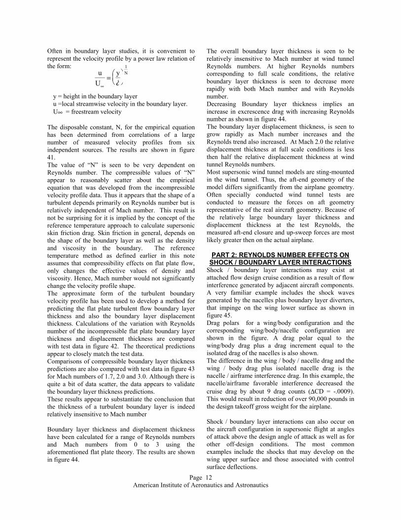
Often in boundary layer studies, it is convenient to represent the velocity profile by a power law relation of the form:
y = height in the boundary layer u =local streamwise velocity in the boundary layer. U∞ = freestream velocity
The disposable constant, N, for the empirical equation has been determined from correlations of a large number of measured velocity profiles from six independent sources. The results are shown in figure 41. The value of “N” is seen to be very dependent on Reynolds number. The compressible values of “N” appear to reasonably scatter about the empirical equation that was developed from the incompressible velocity profile data. Thus it appears that the shape of a turbulent depends primarily on Reynolds number but is relatively independent of Mach number. This result is not be surprising for it is implied by the concept of the reference temperature approach to calculate supersonic skin friction drag. Skin friction in general, depends on the shape of the boundary layer as well as the density and viscosity in the boundary. The reference temperature method as defined earlier in this note assumes that compressibility effects on flat plate flow, only changes the effective values of density and viscosity. Hence, Mach number would not significantly change the velocity profile shape. The approximate form of the turbulent boundary velocity profile has been used to develop a method for predicting the flat plate turbulent flow boundary layer thickness and also the boundary layer displacement thickness. Calculations of the variation with Reynolds number of the incompressible flat plate boundary layer thickness and displacement thickness are compared with test data in figure 42. The theoretical predictions appear to closely match the test data. Comparisons of compressible boundary layer thickness predictions are also compared with test data in figure 43 for Mach numbers of 1.7, 2.0 and 3.0. Although there is quite a bit of data scatter, the data appears to validate the boundary layer thickness predictions. These results appear to substantiate the conclusion that the thickness of a turbulent boundary layer is indeed relatively insensitive to Mach number Boundary layer thickness and displacement thickness have been calculated for a range of Reynolds numbers and Mach numbers from 0 to 3 using the aforementioned flat plate theory. The results are shown in figure 44.
The overall boundary layer thickness is seen to be relatively insensitive to Mach number at wind tunnel Reynolds numbers. At higher Reynolds numbers corresponding to full scale conditions, the relative boundary layer thickness is seen to decrease more rapidly with both Mach number and with Reynolds number. Decreasing Boundary layer thickness implies an increase in excrescence drag with increasing Reynolds number as shown in figure 44. The boundary layer displacement thickness, is seen to grow rapidly as Mach number increases and the Reynolds trend also increased. At Mach 2.0 the relative displacement thickness at full scale conditions is less then half the relative displacement thickness at wind tunnel Reynolds numbers. Most supersonic wind tunnel models are sting-mounted in the wind tunnel. Thus, the aft-end geometry of the model differs significantly from the airplane geometry. Often specially conducted wind tunnel tests are conducted to measure the forces on aft geometry representative of the real aircraft geometry. Because of the relatively large boundary layer thickness and displacement thickness at the test Reynolds, the measured aft-end closure and up-sweep forces are most likely greater then on the actual airplane.
PART 2: REYNOLDS NUMBER EFFECTS ON SHOCK / BOUNDARY LAYER INTERACTIONS
Shock / boundary layer interactions may exist at attached flow design cruise condition as a result of flow interference generated by adjacent aircraft components. A very familiar example includes the shock waves generated by the nacelles plus boundary layer diverters, that impinge on the wing lower surface as shown in figure 45. Drag polars for a wing/body configuration and the corresponding wing/body/nacelle configuration are shown in the figure. A drag polar equal to the wing/body drag plus a drag increment equal to the isolated drag of the nacelles is also shown. The difference in the wing / body / nacelle drag and the wing / body drag plus isolated nacelle drag is the nacelle / airframe interference drag. In this example, the nacelle/airframe favorable interference decreased the cruise drag by about 9 drag counts (∆CD = -.0009). This would result in reduction of over 90,000 pounds in the design takeoff gross weight for the airplane. Shock / boundary layer interactions can also occur on the aircraft configuration in supersonic flight at angles of attack above the design angle of attack as well as for other off-design conditions. The most common examples include the shocks that may develop on the wing upper surface and those associated with control surface deflections.
uU
y N
∞ =
δ
1

Page 13 American Institute of Aeronautics and Astronautics
The presence of a shock / boundary layer interaction is not in itself detrimental. It is only so, if the shock is sufficiently strong to cause separation of the boundary layer. Analyses by the current class of Navier-Stokes CFD codes can provide wonderfully detailed information about the occurrence and the nature of shock / boundary layer interactions that may occur on a complete aircraft configuration. Additional code validation studies, however, are certainly required to establish the validity and robustness of the detailed CFD predictions. In the present discussion we will focus on understand in the general nature of shock / boundary layer interactions on a supersonic aircraft and explore how these interactions might be affected by the Reynolds number differences for a model tested in a supersonic wind tunnel and the corresponding full scale conditions. The general nature of two dimensional and three dimensional flow separations will be discussed. Fundamental classes of shock / boundary layer interactions will be presented. Specific examples of various shock / boundary layer interactions on a supersonic aircraft will be shown. The effect of Reynolds number variations on the fundamental shock / boundary layer interactions will be shown. An approach to judge whether shock induced flow phenomena observed on a model in a supersonic wind tunnel would be significantly different on the corresponding airplane at flight conditions, will be presented.
The general nature of adverse pressure gradient induced two dimensional flow separation is shown in figure 46. The flow within the boundary layer is determined by three causes: it is retarded by the friction at the bounding surface, it is pulled forward by the above free stream flow by the action of viscosity, and in the case of an adverse pressure gradient, it is retarded by the pressure gradient. The flow velocity with in the boundary layer may be insufficient to force its way for very long against the pressure gradient. It is then ultimately brought to rest. Further on next to the wall, a slow back flow in the direction of the pressure gradient may set in. The forward stream then leaves the surface as shown in Figure 46. The upper limit of the boundary layer and the upper limit of the back flow corresponding to the streamline that separates the forward and the reverse flows are also shown. The separation begins where the velocity gradient, du/dy at the wall vanishes. In reference 35, the following intriguing statement is made for both fully laminar flow and for a boundary layer that is turbulent from the stagnation point. “If the pressure distribution is not affected by the separation, then the location of separation is independent of
Reynolds number. The angle that the streamline line AB makes with the surface will depend on the Reynolds number and decreases as the Reynolds number increases. A scale effect on the position of separation arises only for boundary layers that are partly laminar and partly turbulent as a result of the conditions for transition to turbulence.( Ref 35 vol. 2, pp 438)” This would suggest the possibility that the occurrence of sudden boundary layer separations such caused by a strong shock /boundary layer interaction or the formation of a leading edge vortex might be relatively insensitive to Reynolds number variations. The specific details of the flow following the particular separation most likely would be Reynolds number dependent. The classic example of flow separation over a cylinder4
shown in Figure 47 appears to demonstrate this hypothesis. For the Reynolds number range of approximately 104 to 2 x 10⁵, the flow separation is of the laminar nature. The laminar separation point is fixed at an angle of about 80 to 85 degrees. The separation wake is turbulent and the drag coefficient remains constant. As the Reynolds number increases and transition occurs before separation. The separation point moves further around the cylinder and the drag drops rapidly. At a Reynolds number above approximately 5x10⁶, flow over the cylinder is essentially fully turbulent up to separation and the separation point is fixed at approximately 110 degrees. The subsequent drag coefficient appears to level off at a reduced but constant value.
SEPARATED FLOW GENERAL FEATURES Two-dimensional flow separation as shown in figure 48 will result in either an open separation or a closed separation bubble36. The limiting streamline of the upstream flow and the down stream reverse flow streamline meet at a point called a singular point. Consequently this type of flow separation is called singular separation. The singular point is the origin of separation surface separating the upstream flow and the reverse flow. Flow over a 2 dimensional step or a ring around an axi-symmetric body are examples of a closed two dimensional separation bubble. In three dimensional flow two types of flow separation are possible37 as shown in figure 49. These include the previously described singular separation and what is called ordinary separation.

Page 14 American Institute of Aeronautics and Astronautics
In singular separation , two streamlines meet head on and leave the surface as the origin of a bubble separation surface. The requirement for a singular separation is that the shear stress must be zero at the wall. Consequently, the only permissible type of separation in two dimensional or axi-symmetric flow is singular separation. For ordinary separation, the two distinct limiting streamlines near the surface converge tangentially and meet at a point. They then combine and leave the surface in the form of a single streamline. The set of ordinary separation streamlines form a separation surface. Ordinary separation occurs at a down stream pointing cusps in the streamline pattern on a surface. Therefore any down streamline pointing cusps observed in the surface flow patterns on a surface are an indication of ordinary separation. A three dimensional separation bubble is formed by a combination of a single singular point and an array of ordinary separation points. As in two dimensional or axi-symmetric flow, the separation bubble may either be open or closed. Similarly, three dimensional separated flow can reattach to the surface at either singular attachment points or ordinary attachment points. Ordinary attachment points would appear as upstream facing cusps in the flow patterns. Examples of three dimensional flows with separation and reattachment are shown in sketches in figure 50. The closed separation bubble is formed by a single singular separation point and an array of ordinary separation points. The bubble surface reattaches by means of a singular reattachment point and numerous ordinary reattachment points. A classic example of three dimensional separation is the flow against an obstacle projecting from a flat plate. As Shown in figure 51, the flow is forced to separate in a broad bubble surrounding the root of the cylindrical obstacle. The point S on the stagnation surface streamline is the singular separation point. The remainder of the separation line is a sequence of ordinary separation points. The surface of separation forms a separation bubble around the cylinder. The secondary outward flow caused by the streamline curvature results in a skewness of the boundary layer. This flow pattern profoundly modifies the outer flow characteristics. Hence it is apparent that the features of this type of flow situation would be very dependent on Reynolds number. Figure 52 shows the surface pressure distribution and flow particle trace patterns computed by a Navier-Stokes code for the flow over a rectangular nozzle at a low supersonic Mach number. The particle traces indicate that the flow over the upper surface flap
separates near the aft end forming an open separation bubble. The singular separation point and the ordinary separation points that form the separation bubble are quite apparent in the calculated particle trace patterns. The cross flow over the side plate separated and formed a side vortex. The general forms of the surface flow pattern for swept-shock / boundary layer interactions are shown in figure 53. For attached flow, the pressure gradient in the transverse direction encountered by the flow passing through the shock deflects the boundary layer flow through an angle greater than the free stream flow deflection angle. When the surface flow is deflected by an angle large enough to becomes aligned with the inviscid shock, incipient separation is said to occur37. In fact, the alignment of the surface flow with the inviscid shock is considered a necessary condition for the establishment of incipient separation but not necessarily a sufficient one. For complete separation, the surface flow is deflected at large enough angle to intersect the inviscid shock and then tangentially merges with the deflected upstream flow. The characteristic cusp pattern indicating ordinary separation is once again evident. The characteristics of the flow in a swept-shock/boundary layer interaction can also be inferred from the skin friction lines as shown in figure 54. Even in the case of a weak shock/boundary layer interaction, the skin friction lines are deflected substantially more then the inviscid streamlines. The skin friction lines do not converge and hence there is no separation. The view along the interaction along the shock is similar to that of a two dimensional weak normal shock / boundary layer interaction. When the shock strength has increased sufficiently to separate the flow, the skin friction lines appear as on the right side of figure 54. In this example, a separation bubble develops at the three dimensional separation line upstream of the inviscid shock wave position. Skin friction lines emanating from the reattachment line behind the shock pass through the inviscid shock position and merge asymptotically with the separation line. The upstream skin friction lines also merge with the separation line. The view of the interaction along the shock wave indicates a lambda foot at the shock and a vortical slip line passing downstream of the triple point.

Page 15 American Institute of Aeronautics and Astronautics
FUNDAMENTAL CLASSES OF SHOCK / BOUNDARY LAYER INTERACTIONS. In order to develop an understanding of Reynolds number effects on off-design conditions in which shock / boundary layer interactions might occur, we shall identify the fundamental class of shock boundary layer interactions that typically occur on supersonic aircraft. Then available experimental data relating to each fundamental class of interaction will be used to identify how Reynolds differences affect the various interactions. The fundamental class of shock / boundary layer interactions that may be experienced by a supersonic aircraft at various conditions within its supersonic flight envelope are shown in figure 55. These include glancing shock waves, compression corners, incident shock waves and crossing or interfering shocks. The glancing shock wave is a swept and nearly vertical shock that may be generated by a number of different sources such as:
• Coalescence of wing inboard compressions into an upper surface shock
• Body compression shocks • Wing apex / body junction shock • Horizontal or vertical shocks at the junction on
the body • Shocks from wing mounted vertical tails • Nacelle diverter shock falling on the wing
Compression corner shocks are swept shocks at the hinge lines when control surfaces are deflected. Another source of a compression type shock occurs at the trailing of wing, vertical, horizontal or canard surface that has a supersonic trailing edge. Incident shocks are shocks that impinge on another surface by an adjacent planar or three dimensional surface that created the shock. Incident shocks occur:
• In two dimensional inlets • Axi-symmetric spike inlet • Nacelle cowl shocks impinging on the wing • Shock cancellation concepts such as supersonic
bi-plane, parasol wing.
The fourth class of shocks include are crossing or interfering shocks which are a combination of the other fundamental shocks. Examples include shocks created on a wing by an adjacent set of nacelles and diverters, or in the case of a military airplane, externally mounted adjacent stores or weapons
COMPRESSION CORNER SHOCK / BOUNDARY LAYER INTERACTIONS
Two examples of shock that can develop on a supersonic aircraft that are variations of a compression shock are shown in figure 56. These include the shocks that would occur as the leading edge and trailing flaps would be deflected at off design supersonic conditions, and the trailing edge shock for a wing with a supersonic trailing edge. The wing trailing edge shock develops to allow the wing upper surface pressures to adjust to the free stream static pressure 8,9. Empirical correlations of separation data for compression corners as shown in the figure indicate that a pressure rise exceeding 1 + 0.3 MN
2 can result in flow separation. Additional experimental studies have shown that the sweep of a compression corner can be accounted for by the use of the local normal Mach number, MN. The pressure ratio for incipient separation for a compression corner, therefore increases with the local Mach number and decreases with increases in local sweep. Figure 57 contains results of additional empirical studies36 that explored the effect of Reynolds number on the incipient separation pressure ratio and on the corresponding deflection angle for incipient separation. The results in this figure imply that if a compression corner type separation occurs on a typical supersonic model, then the corresponding separation will occur on the full scale airplane. The principal variable controlling pressure distribution in the separated flow irrespective of Mach and Reynolds Number is the location of transition relative to the separation and the reattachment positions as illustrated in figure 58. Pure laminar separations are characterized by transition down stream down stream of the reattachment position. This type of separation is steady at supersonic speeds. The shape of the pressure profile for laminar separation is characterized by an initial pressure rise followed by a rather large pressure plateau followed by a rise to the inviscid shock pressure level. The laminar separation is not strongly dependent on Reynolds. The level of the plateau pressure is, however, greater at lower Reynolds numbers. Transitional separations are characterized by transition occurring between separation and reattachment. This type of flow is generally unsteady and often depends on Reynolds number to a great extent. An abrupt pressure rise often occurs at the location of transition especially if transition occurs just before reattachment. Turbulent separations are characterized by transition occurring upstream of separation. Turbulent separations are quite steady and are not strongly dependent on Reynolds number. The pressure rise in a turbulent

Page 16 American Institute of Aeronautics and Astronautics
separation does not have a plateau level but rather a point of inflection as the pressure rises. The extent of the separation region is much smaller for a turbulent boundary layer. The effect of Reynolds number variations on the length of the separation regions and on the pressure separation region pressure distributions 36 are shown in figure 59. The length of the separation region and the overall separation pressure distribution shape for laminar separation is seen to be insensitive to Reynolds number. The plateau pressure level is reduced by increasing Reynolds Number. The length of the separation region and the plateau pressure varies significantly with Reynolds number for transitional separation. The characteristics of the separation region for turbulent separation is quite insensitive to Reynolds number The results shown in the figure correspond to separation induced by a compression corner. However the general conclusions about the effects of Reynolds Number on the separation region characteristics are equally appropriate to the other fundamental types of shock induced separations. It is anticipated that the flow over a typical HSCT will essentially be fully turbulent flow. Hence it is important that tests on a small scale supersonic wind tunnel model must insure that turbulent flow conditions exist in any area where shock / boundary layer interactions are likely to occur. The separations on the model and on the full scale airplane will then occur at the same conditions. Furthermore, the size of the separation regions and the pressure distribution in the regions will also be similar for both the model in the wind tunnel and the airplane in flight.
INCIDENT SHOCK / BOUNDARY LAYER INTERACTIONS
Results of experimental correlations 36 of the effect of Reynolds and Mach number on the pressure ratio and deflection angle for incipient separation induced by unswept incident shocks, are shown in figure 60. The experimental data Indicate that the pressure rise and deflection angle for incipient separation increase with Mach number. The relation between the pressure ratio and deflection angle suggests that the shock reflection magnification is about 1.7 instead of 2 for a perfect reflection of a shock from an adjacent surface. The incipient deflection angle decreases with Reynolds number and appears to approach a limiting deflection angle of approximately 7.5 degrees. A limiting shock deflection angle of 7.5 degrees and a shock reflection factor of 1.7 was used to derive the following empirical equation for the high Reynolds number limiting pressure ratio for incipient separation
caused by incident shocks in terms of the local Mach number, MLOC, and the Sweep angle of the incident shock, LS.
The lower the local Mach number in the region of the incident shock, the less sensitive is the pressure ratio for incipient separation GLANCING SHOCK / BOUNDARY LAYER INTERACTIONS Figure 61 shows an example of the formation of a glancing shock on a highly swept supersonic wing8. The oil flow characteristics indicate separated flow behind a strong body induced shock. The oil flow illustrates the characteristics of the surface flow as previously described for a general swept shock / boundary layer interaction. The separation line, as indicated by the merged surface flow streamlines, is seen to lie substantially forward of the calculated inviscid shocks positions. The separated flow characteristics indicates an open separation bubble resulted, since there is no apparent indication of a reattachment line on the wing surface. Figure 62 shows another example of a glancing shock that is formed by coalescence of weak compression waves on upper surface of a wing8,9. This flow is associated with flow conditions near the inboard portion of the wing. The formation of this type of shock is not in itself necessarily undesirable. It is only if the shock strength is sufficiently strong to cause separation. The shock strength is defined as the ratio of the static pressure after the shock to the static pressure before the shock, P2/P1. Results of correlations of experimental wind tunnel data indicates that an incident shock will induce separated flow if the pressure ratio exceeds 1.5. Figure 63 contains a comparison of the limiting higher Reynolds number shock separation criteria for a glancing shock, incident shock, and both swept and unswept compression shocks. It is seen that the ability of a turbulent boundary layer to withstand the various fundamental types of shock interactions is strongly dependent on the Mach number. The sweep of the shock is seen to be very significant in reducing the ability of a boundary layer to avoid separating behind a shock. The effect of the local pressure field on the strength of a shock / boundary layer interaction is shown in figure 64. A shock of specified pressure rise, ∆CP, is more likely to cause separation when impinging on an area of low pressures, such on the upper surface of a wing, then when impinging on a area of higher pressures as on the lower surface of a wing.
( )2
1
2 cos065.0313.2 sLOCMPP Λ+=

Page 17 American Institute of Aeronautics and Astronautics
NACELLE –DIVERTER CROSSING SHOCK INTERACTIONS
Figure 65 shows examples of crossing or interfering shock interactions. The upper portion of the figure shows both test data and CFD computations for interactions caused by two wedges mounted on a flat surface. The lower pictures show wind tunnel flow visualization pictures of the flow between adjacent nacelles on an HSCT type configuration. Calculations of Navier-Stokes and Euler predictions of wing pressure distributions on a supersonic wing/body/nacelle configuration are compared with the corresponding wind tunnel test data in Figure 66. The primary differences between the viscous and inviscid surface pressures are on the lower surface of the wing in the region influenced by the nacelles. The predicted inviscid surface shocks are seen to be much stronger then those predicted by the Navier-Stokes code. The Navier-Stokes predicted shocks are both weaker then the inviscid shocks and also move further upstream. This implies that the nacelle/diverter shocks actually separated the local flow. The Navier-Stokes prediction are seem to closely match the test data. Navier Stokes predictions of the wing pressure distributions at wind tunnel and at full scale conditions are shown in figure 67. The stronger viscous effects at the wind tunnel Reynolds numbers creates a somewhat different shock pattern in the vicinity of the nacelles at station 32.6%. However the predictions at full scale Reynolds number are much more similar to the viscous predictions at wind tunnel conditions then to the corresponding inviscid predictions. At full scale conditions there exists a pair of reflected shocks and expansions in addition to the shock off the nacelle inlets and diverter. At the wind tunnel Reynolds numbers these secondary shocks are smeared out and appear to vanish. At station 41.3%, the flight Reynolds number results show a much stronger pair of shocks as well as a stronger expansion region. The difference in wind tunnel to flight has very little effect on the upper surface pressures for this configuration. The calculated nacelle flow field shocks strengths at various wing stations that are indicated in the previous two figures, are shown in the shock amplification chart in figure 68. The strength of the inviscid shock is seen to be much larger then the glancing shock separation criteria. The viscous shocks are seen to essentially match the separation criteria as one might expect to occur after a local boundary layer separation.
Figure 69 contains Navier Stokes predictions of the pressure drag near zero lift and near cruise for the previously shown, wing/body/nacelle configuration. The calculations include both wind tunnel and full scale Reynolds number conditions. The full scale pressure drag is approximately one drag count lower then the corresponding wind tunnel drag levels at the cruise CL and Mach number. The full scale drag levels are approximately two tenths of a drag count less then the wind tunnel levels near zero lift. The effect of the Reynolds number increase is seen to be slightly beneficial and is most likely associated with a reduction in the boundary layer displacement thickness at the larger Reynolds numbers. Another example of Experimental and computed pressure distributions on the lower surface of a wing / body / nacelle configuration is shown in figure 70. The data shown in the figure are the results for a non spilling flow thru nacelle installation. This case was the baseline reference case for an Investigation38 of engine unstart effects at supersonic speeds. The shock locations predicted by the Navier Stokes code matches the experimental shock location. The viscous shock location lies forward of that predicted by the inviscid code because of a mild separation caused by the nacelle-diverter shock on the wing. Figure 71 contains a comparison of the experimentally determined nacelle-on-wing shock location together with the Euler predictions of the wing surface pressures and the theoretical shock locations for the condition of an unstarted outboard engine. Comparisons of the unstarted engine pressure distribution in this figure with the pressure distribution for the flow-through-nacelle on the previous figure shows a dramatic forward movement of the nacelle-on-wing shock system. The computed inviscid shocks strengths greatly exceeded the glancing shock separation criteria. The forward location of the experimental shock relative to the inviscid shock is due to the separation of the boundary layer caused by the shock interaction. A common HSCT design criteria affecting the location of the nacelles on a wing is that the unstart of one engine will not cause a mutual unstart of the adjacent engine. In the example shown in figure 71 , the inviscid calculations would have implied that the design criteria was satisfied by this installation. However, the wind tunnel data results indicate that mutual unstart was indeed a possibility since the shock from the unstarted outboard engine passed in front of the adjacent inboard engine. Based on the previous discussions of Reynolds number effects on shock boundary layer interactions, it is expected that mutual unstart would be a design risk for the full scale configuration.
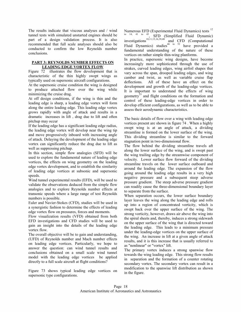
Page 18 American Institute of Aeronautics and Astronautics
The results indicate that viscous analyses and / wind tunnel tests with simulated unstarted engines should be part of a design validation process. It is also recommended that full scale analyses should also be conducted to confirm the low Reynolds number conclusions.
PART 3: REYNOLDS NUMBER EFFECTS ON LEADING EDGE VORTEX FLOW
Figure 72 illustrates the flow development that is characteristic of the thin highly swept wings as typically used on supersonic aircraft configurations. At the supersonic cruise condition the wing is designed to produce attached flow over the wing while minimizing the cruise drag. At off design conditions, if the wing is thin and the leading edge is sharp, a leading edge vortex will form along the entire leading edge. This leading edge vortex grows rapidly with angle of attack and results in a dramatic increases in lift , drag due to lift and often pitchup may occur If the leading edge has a significant leading edge radius, the leading edge vortex will develop near the wing tip and move progressively inboard with increasing angle of attack. Delaying the development of the leading edge vortex can significantly reduce the drag due to lift as well as suppressing pitchup. In this section, simple flow analogies (SFD) will be used to explore the fundamental nature of leading edge vortices, the effects on wing geometry on the leading edge vortex development, and to establish the similarity of leading edge vortices at subsonic and supersonic speeds. Wind tunnel experimental results (EFD), will be used to validate the observations deduced from the simple flow analogies and to explore Reynolds number effects at transonic speeds where a large range of test Reynolds numbers is possible. Euler and Navier-Stokes (CFD), studies will be used in a synergistic fashion to determine the effects of leading edge vortex flow on pressures, forces and moments. Flow visualization results (VFD) obtained from both EFD investigations and CFD studies will be used to gain an insight into the details of the leading edge vortex flow. The overall objective will be to gain and understanding, (UFD) of Reynolds number and Mach number effects on leading edge vortices. Particularly, we hope to answer the question: can wind tunnel results and conclusions obtained on a small scale wind tunnel model with the leading edge vortices be applied directly to a full scale aircraft at flight conditions? Figure 73 shows typical leading edge vortices on supersonic type configurations.
Numerous EFD (Experimental Fluid Dynamics) tests 12
to 14, 41 to 45, SFD (Simplified Fluid Dynamic) investigations10,11,15,16,39,40 and CFD (Computational Fluid Dynamics) studies46 to 52 have provided a fundamental understanding of the nature of these vortices on rather simple thin-wing planforms. In practice, supersonic wing designs, have become increasingly more sophisticated through the use of strakes, curved leading edges, wing airfoil shapes that vary across the span, drooped leading edges, and wing camber and twist, as well as variable cruise flap deflections. All of these have an effect on the development and growth of the leading-edge vortices. It is important to understand the effects of wing geometry53 and flight conditions on the formation and control of these leading-edge vortices in order to develop efficient configurations, as well as to be able to assess their aerodynamic characteristics. The basic details of flow over a wing with leading edge vortices present are shown in figure 74 . When a highly swept wing is at an angle of attack, a dividing streamline is formed on the lower surface of the wing. This dividing streamline is similar to the forward stagnation point in two-dimensional flow. The flow behind the dividing streamline travels aft along the lower surface of the wing, and is swept past the wing trailing edge by the streamwise component of velocity. Lower surface flow forward of the dividing streamline travels on the lower surface outboard and around the leading edge. The expansion of the flow going around the leading edge results in a very high negative pressure and a subsequent steep adverse pressure gradient. The steep adverse pressure gradient can readily cause the three-dimensional boundary layer to separate from the surface. When separation occurs, the lower surface boundary layer leaves the wing along the leading edge and rolls up into a region of concentrated vorticity, which is swept back over the upper surface of the wing. The strong vorticity, however, draws air above the wing into the spiral sheets and, thereby, induces a strong sidewash on the upper surface of the wing that is directed toward the leading edge. This leads to a minimum pressure under the leading-edge vortices on the upper surface of the wing. An increase in lift at a given angle of attack results, and it is this increase that is usually referred to as "nonlinear" or "vortex" lift. The primary vortex induces a strong spanwise flow towards the wing leading edge. This strong flow results in separation and the formation of a counter rotating secondary vortex. The secondary vortex can result in a modification to the spanwise lift distribution as shown in the figure.

Page 19 American Institute of Aeronautics and Astronautics
The typical surface streamline pattern on the wing upper surface shows the central potential flow area as well as the streamline directions under the primary and the secondary vortices. The size and shape of the vortex flow is indicated by the measurements of total pressure in the flow field. A simplified flow analogy representing the development of the leading edge vortex on thin sharp leading edge slender delta wings was formulated by E. C. Polhamus15,16. The leading edge suction analogy equates the local vortex lift to the local theoretical leading edge suction force at each spanwise station across the wing. The local vortex normal force at any spanwise station and angle of attack is determined by rotating the corresponding local theoretical leading edge suction force 90 degrees to be normal to the local chordline. For a thin sharp edge flat lifting surface, the total vortex normal force is therefore equal to the total suction force. The local leading edge suction force and therefore the total leading edge vortex strength increase with the square of the angle of attack. The leading edge suction analogy provides a simple technique to calculate vortex lift , pitching moment and drag on thin sharp edge flat slender wings. This suction analogy has subsequently been extended to arbitrary thin sharp edge slender planforms39,40. Figures 75 show comparison of suction analogy lift predictions with test data. The agreement between the predictions and the theory is very good. The lift with vortex flow is seen to be substantially greater then just the potential flow lift. The drag due to lift factor which is defined as the ratio of drag due to lift divided by the square of the lift coefficient is shown for the family of delta wings in figure 76. The drag due to lift is determined as the component of the combined potential lift plus vortex lift vector acting in the streamwise direction. The experimental drag due to lift obtained for a family of thin sharp leading edge wings is compared with leading edge suction analogy predictions. The theoretical predictions again are seen to closely match the test data. Two other sets of drag due to lift calculations are shown in the figure for reference. These include minimum drag due to lift corresponding to the leading edge suction force acting in the plane of the wing, and the drag due to lift without account for the leading edge suction force. This type of comparison provides an indication of the relative magnitudes on the induced drag vortex lift. The drag due to lift with vortex flow is seen to be significantly higher then that achieved with attached flow.
Through the use of the suction analogy39, it has been shown that the development of vortex lift occurs also at supersonic speeds as long as the leading edge of the wing is swept behind the free stream Mach line and the planform subsequently has a subsonic leading edge. Figure 77 contains an example of predictions of vortex lift and drag due to lift at supersonic speeds along with the corresponding test data. LEADING EDGE VORTEX FORMATION WITH
ROUND NOSE AIRFOILS The leading edge suction analogy was extended to slender wings with round edges and thick sharp edges using a residual suction concept 10. With the residual section concept, the local leading edge suction force is compared with the local airfoil nose pressure drag force which acts in the plane of the wing. The round nose pressure force does not vary with angle of attack whereas the local leading edge suction force varies with the square of the angle of attack. Therefore, at some angle of attack, the magnitude of the suction force will equal and begin to exceed the local nose pressure drag force. This angle of attack is defined as the local separation angle of attack at which the leading edge vortex first starts to form at that station. The strength of the local leading edge vortex is then determined as the square of the difference between the actual angle of attack and the local separation angle of attack. This local vortex lift for a wing with a round leading edge, is therefore only a portion of the total local leading edge suction force. The difference between the total suction force and the portion converted into vortex lift is assumed to act in the local chord plane as a residual leading edge suction force. The residual suction method predicts the inboard movement of the leading edge vortex with angle of attack for slender wings with round nose airfoils or sharp edge wings with finite thickness, as well as the resulting lift, drag and pitching moment. Figure 78 shows lift predictions using the original thin sharp edge suction analogy theory and the extended round nose residual suction theory with test data for two similar wing planforms. One wing had a thin sharp edge airfoil and the other wing had a thick round nose airfoil. The predictions agree well with the test data and illustrate the effect of the round nose in suppressing the leading edge vortex formation. The effect of the round nose is to reduce both the total wing lift and the corresponding wing drag to lift10. The residual suction method was subsequently used to study the effects of airfoil shape, thickness distribution, wing camber and twist, flap deflections as well as planform variations on vortex flow11. An extensive series of wing tunnel tests were conducted as part of a joint NASA Langley / Boeing research

Page 20 American Institute of Aeronautics and Astronautics
effort43,44 to provide an extensive database for use in validating theoretical aerodynamic and aeroelastic prediction theories. The wind tunnel model geometry consisted of an arrow wing plus body configurations including flat, twisted and cambered wings, as well as a variety of leading and trailing edge control surface deflections. The tests were conducted at subsonic, transonic and supersonic Mach numbers. The model geometry and a typical airfoil section are shown in figure 79 along with sample data obtained at Mach = 0.85 for the flat wing planform with a round nose airfoil. The variation of the lifting pressure coefficient at 2.5% local chord is shown for a typical spanwise station. The general characteristic of the pressures observed near the leading edge included a nearly linear variation of the lifting pressure coefficient with angle of attack up to an angle of attack where a break in the pressure curve would occur. As shown in the figure, the pressure break angle of attack at every spanwise station correlated very well with the theoretical prediction local separation angle which is defined as the angle of attack, αS, at a station at which the leading edge vortex first appears. The effect of the round nose airfoil is to create a range of angle of attack at which attached flow will be retained. For a flat symmetric wing, this region is symmetric for both positive and negative angles of attack. Results of studies11 of leading edge flap deflections on the formation of the leading edge vortex for an arrow wing with sharp thin airfoils and an arrow wing with round nose airfoils are shown in figure 80. For the flat wing with a sharp thin airfoil section, the leading edge flow is only attached for zero degrees angle of attack. A leading edge vortex will form along the entire leading edge at any other angle of attack. For a constant flap deflection of 15 degrees across the span, the attachment angle of attack is pushed up to some non zero degree angle of attack that varies across the span. At a constant angle of attack, the leading edge vortex may actually occur on the wing upper surface for a portion of the span and then wrap around to the wing lower surface for the remaining portion of the span. As shown in the figure, it is possible to select a flap schedule across the wing span such that the attachment line for a thin sharp edge wing is constant across the span for some fixed angle of attack other then zero degrees angle of attack. The effect of the round nose airfoil is to create a dead band region of attached flow that is symmetric about the corresponding thin sharp edge wing spanwise attachment line. The effect of flap deflections for a wing with round nose airfoils is to push the attached region up to different angles of attack across the span.
Wing camber and twist, similarly would simply shift the attachment region set by the wing leading edge radius to different angles of attack across the wing span. The effect of outboard leading edge flap deflections on the surface streamline pattern for an HSCT type wing planform is shown in Figure 81. The wing planform was cambered and twisted for optimum supersonic cruise drag. The airfoil shapes across the inboard wing had round leading edges out to the leading edge break, outboard of the leading edge break, the airfoils were rather thin with sharp leading edges. Without any leading edge flap deflections, the flow was attached along the inboard leading edge but separated on the outboard portion of the planform and formed a leading edge vortex on the outer panel. With the outboard flaps deflected, the flow on outboard wing panel also remained attached. Using the aforementioned approach of identifying the initial leading edge vortex formation at any spanwise station by the break in the lifting pressure variation with angle of attack, the separation boundaries for the swept arrow wing are shown for supersonic Mach numbers in Figures 82 and 82. Comparing these results with the corresponding subsonic separation boundary shown in Figure 79, indicates that the increased Mach numbers reduced the angle of attack range for attached flow. The general conditions leading to the formation and growth of a leading edge vortex at subsonic speeds are similar to those at supersonic speeds provided the leading edge is subsonic. Investigations of the effects of Reynolds number variations on leading edge vortices at subsonic speeds should, therefore, yield observations and conclusions that are applicable to similar supersonic flows. Consequently we will use results from of a number the experimental and computational of studies on the effects of Reynolds number variations on leading edge vortices at subsonic speeds, and develop conclusions that should be equally applicable to supersonic speeds. An extensive wind tunnel test program45 of a 65O delta wing model with interchangeable leading edges was conducted in the NASA Langley National Transonic Facility, NTF. The objective was to investigate the effects of Reynolds numbers and Mach number on slender-wing leading-edge vortex flow with four values of leading edge bluntness. The experimental data included surface pressure measurements, and measurements of normal force and pitching moment. The wing planform and various leading edge geometries are shown in figure 84.

Page 21 American Institute of Aeronautics and Astronautics
Measurements of the lifting pressures coefficients near the leading edge of the wing are shown in the figure for a typical wind tunnel Reynolds number. The attached flow boundary that was determined from the breaks in the lifting pressure coefficient curves, is also shown. The sharp edge wing apparently achieves attached flow over a small range of angle of attack because of the overall thickness of the wing and the rather steep angles of the sharp edge. Similar pressure measurements for the medium round nose geometry are shown in figure 85 for the same test conditions. The separation boundary determined for this geometry is also shown. The separation boundaries for the sharp leading edge and the medium leading edge geometries are compared in figure 86 The medium round nose geometry is seen to provide approximately and additional 4 degrees angle of attack over which attached flow is retained. Experimental results obtained with the medium nose radius geometry are shown in figures 87 through 90 for increasing Reynolds number from typical wind tunnel conditions to approximately full scale conditions. The set of lifting pressure curves for each of the test Reynolds numbers, all show the same general characteristic trends with angle of attack. The lifting pressures measures near the leading edge across the wing span all vary linearly with angle of attack up to some departure angle corresponding to a break in the lifting pressure curve. These departure angles were used to define the spanwise angle of attack range for attached flow and thereby define the inboard movement of the origin of the leading edge vortex with angle of attack. The experimentally determined separation boundaries obtained for the medium round nose geometry shown in figures 87 through 90 are compared in figure 91. These results indicate that the separation boundary for attached flow and therefore the spanwise movement of the origin of the leading edge vortex with angle of attack, is relatively insensitive to Reynolds number variations from wind tunnel to flight conditions. Figure 92 shows the variation of normal force and pitching moment with angle of attack for the NASA 65O delta wing. The data shown in the figure also correspond to the number of Reynolds numbers from wind tunnel to flight conditions. The lift and the pitching moment show little effect for the variations of Reynolds numbers.
THEORETICAL ANALYSES OF LEADING EDGE VORTEX FLOWS
The detailed characteristics of the flow field associated with leading edge vortices are indeed very complicated. The formation of the leading edge vortex is in itself a viscous related phenomena since boundary layer separation from the surface of a wing is the basic origin
of the leading edge vortex. The leading edge vortex once formed, forms a highly concentrated region of vorticity that decays relatively slowly downstream and consequently, behaves very much like a inviscid potential flow phenomena. The inviscid like nature of the developed vortex flows allowed the development of early potential flow computational models that captured some of the characteristics of leading edge vortices and their effects10. Some of the earliest analytical models included the two-dimensional cross flow models as shown in figure 93. The earliest crossflow leading edge vortex models were followed by that represented the complete three dimensional vortex by either a series of discrete vortices of by a complete three dimensional modeling of the vortex sheet as shown in figure 94. These simplified representation of the leading edge vortex lead to reasonably good correlations with test data for thin sharp edge wings as shown in the figure. More recently, numerical solutions to the Euler equations have led to useful numerical computations of the flow characteristics of leading edge vortices on thin sharp edge wings. In this case, the numerical viscosity in the solution process of the Euler equations, no matter how small, is sufficient to result in the formation and growth of the leading edge vortices. Figure 95 contains comparisons of Euler spanwise pressure predictions with experiment17 at supersonic speeds for a thin sharp 75O delta wing at an angle of attack of 12O. At both analysis Mach numbers, the experimental data and the theoretical predictions indicate leading edge separation that resulted in the formation of a leading edge vortex on the upper surface. The most notable difference between the Euler predictions and the experimental data is the lack of a secondary vortex in the Euler predictions. The secondary vortex is a local viscous phenomena which can not be predicted with the an inviscid code. At the lower Mach number, Mach 1.7, The effect of the secondary vortex results in two local pressure peaks. At the higher Mach number, Mach 2.8, The secondary vortex appears to have little effect on the pressure distributions. It appears that the effects of the secondary vortex vanish with increasing Mach Number. Theoretical and experimental results for the flat wing at 12O degrees angle of attack and for 8O of yaw are shown in figure 96 for Mach 1.7 and 2.8. The pressure distributions and flow field features are shown for both the windward (left) side and the leeward (right) side.

Page 22 American Institute of Aeronautics and Astronautics
For both cases the asymmetry of the flow due to yaw is evident although the flow fields are quite different for the two Mach numbers. At the lower Mach number, leading edge separation occurred on both the windward and leeward edges. The windward edge separation developed into a separation bubble that lies close to the wing surface. The leeward side separation developed into a conventional leading edge vortex. At the higher Mach number, The flow is attached on the windward side and develops a leading edge vortex on the leeward side. The asymmetry in flow fields for both Mach numbers leads to rolling moment due to the yaw condition. For both of the Mach numbers, the Euler predictions agree quite well with the experimental results. With a round nose airfoil, the action of viscosity in the boundary layer will determine where the local flow separates and not just at a geometric singularity as in the case of a sharp leading edge. It is reasonable to expect that for highly swept wings with round leading edges, the action of the viscosity leading to the flow separation and subsequent leading edge vortex formation must be captured in the solution process. This requires a solution of the Navier-Stokes equations. Euler and Navier Stokes laminar flow calculations have been made46,47 of the flow over a cropped 65O flat delta wing with a 5% round nose airfoil section. The results have been compared with test data obtained at Mach 0.85 and a Reynolds Number based on the root chord of 2.38 x 10⁶. Figure 97 shows a comparison of flow pathlines near the wing surface, wing isobars, total pressure contours and vorticity contours for the Euler and the Navier-Stokes solutions. The numeric vorticity inherent in the Euler solution process allows a leading edge vortex development to occur even for the analysis of wings with round edge airfoils. The origin of the leading edge vortex predicted by the Euler code is seen to be quite different then that predicted by the Navier-Stokes Solution. In the viscous solution the leading edge vortex at the analysis angle of attack is seen to start at the wing apex. In the Euler solution, the leading edge vortex starts at about one quarter chord down from the wing apex. The Euler solution and the Navier Stokes Solution both show evidence of secondary vortices that lie close to the wing leading edge and below the primary vortices. The secondary vortex in the case of the Euler Solution is caused by a cross flow shock. The secondary vortex in the case of the Navier-Stokes solution is a more correct representation of the flow physics and is caused by separation of the boundary layer induced by the strong cross flow under the primary vortex.
Figure 98 provides some insight into the differences that might be encountered when applying an Euler code for prediction the flow characteristics on a highly swept round nose airfoil. The figure includes a comparison of the wing pressures calculated by an Euler analyses and a Navier-Stokes analyses46, with test data obtained at Mach 0.85 and a Reynolds Number based on the root chord of 2.38 x 10⁶. The Navier-Stokes predictions appear to predict the location of the primary vortex and the minimum induced pressures quite well. The overall Navier-Stokes predictions agree much better with the test data then do the Euler code predictions. The Navier-Stokes predictions however, did not appear to properly capture the details of the secondary vortex interactions which occur in the region close to the leading edge. This is evident by the differences in the predicted and measured upper surface pressures near the wing leading edge in this figure. An extensive computational study48 was conducted in which the CFL3D Navier-Stokes code was used with the Spalart-Allmaras turbulence model to predict the flow characteristics of the 65O delta wing with the medium leading edge radius and the round leading edge radius that were previously discussed, (figures 84 through 92). The analyses were made for Mach = 0.85 and a range of Reynolds numbers from wind tunnel to full scale flight conditions. Calculated surface streamlines are shown in figure 99. The predicted streamlines are essential identical for the compute Reynolds number range of 6 x 10⁶ to 120 x 106. The surface stream lines clearly show the primary leading edge vortex, the induced secondary vortex and separation near the wing trailing where the thickness rapidly closed to a sharp edge. Computed spanwise pressure distributions are compared with experimental data for an attached flow condition and for a separated flow condition in figure 100. The theoretical pressures for the attached flow condition agree well with the test data. For the higher angle of attack where leading edge separation occurred over essentially the entire leading edge, the theory appears to correctly predict the overall vortex lift but does not predict the effect of the secondary vortex extremely well. Experimental and theoretical pressure distributions for an angle of attack of 7O where the flow remains attached are shown in figure 101 for the Reynolds number range of wind tunnel to flight. Both theory and experiment indicate that the pressure distributions in flight are the same at a typical wind tunnel Reynolds number.

Page 23 American Institute of Aeronautics and Astronautics
Similar comparisons are shown for an angle of attack of 12O for which a leading edge vortex occurs over the entire leading edge in figure 102. The theoretical pressure distributions are essentially identical for all of the computed Reynolds numbers. Although the theoretical and the experimental pressures differ in the region influenced by the secondary vortex, the experimental pressure distributions vary only slightly over the entire range of Reynolds numbers. It would appear that wind tunnel data obtained for this wing geometry would be very applicable for a corresponding full scale wing geometry at flight conditions. Results of a Navier-Stokes parametric computational study49 that was conducted to investigate the effects of leading edge radius, leading edge camber, Reynolds number and boundary layer model on the flow characteristics of a 65O delta wing at Mach = 1.6 are shown in figures 103 through 106. Analyses were made for two different angles of attack that included 4O and 8O. The smaller angle of attack, according to the leading edge vortex formation boundary shown in figure 10, should result in attached flow even for the sharp leading edge geometry. At the larger angle of attack, a leading edge vortex is expected to occur. Figure 103 shows results of the Navier-Stokes analyses for various leading edge geometries at the two angles of attack. The leading edge geometries included a sharp edge, an elliptic nose geometry and a blunt round nose geometry. At 4 degrees angle of attack, the pressure distribution on the sharp nose geometry shows a slight inflection that corresponds to a leading edge separation bubble. Both round nose geometries had attached flow at the lower angle of attack. At 8 degrees angle of attack, leading edge vortex flow occurred on all three geometries. It does appear that the round nose geometries did result in a reduction in the vortex lift which indicates that the formation of the leading edge vortex was indeed delayed. The effect of increasing leading edge camber with the medium nose radius elliptic geometry was analyzed at an angle of attack of 8 degrees with Navier-Stokes turbulent flow analyses. The results as shown in figure 104, indicate that increased nose camber can be effective in delaying the formation of the leading edge vortex. The results are consistent with the explanation on the benefits of leading edge radius and nose camber as offered by the residual suction analogy in conjunction with figure 80. The leading edge radius creates a region of angle of attack for which the flow remains
attached and the effect of nose down camber is to shift the region of attached flow to higher angles of attack. The 4O camber shown in figure 104 was not sufficient to delay the leading edge vortex formation. The 8O degree camber shifted the attached flow region such that a leading edge separation just started to form. The largest camber resulted in attached flow at the analysis station. The effect of a moderate increase in Reynolds number on the elliptic nose configurations with and without nose camber, was also analyzed with the turbulent flow model. The computed pressure distributions are shown in figure 105 for 8O angle of attack. The results for the uncambered wing where the leading edge separation occurs, imply that increasing the Reynolds number slightly did not affect the formation of the leading edge vortex. The minimum pressure peak on the wing, however, did increase. The flow on the cambered wing was an attached flow case The overall effect of the Reynolds number increase for this attached flow case was also rather small. The increase in Reynolds number appears to have resulted in a slight separation at the base of the recompression that occurred near the leading edge as evidenced by the slight inflection in the pressure curves. The effects of turbulent flow versus laminar flow was investigated through the use of different viscous flow models in the Navier-Stokes analyses. The pressure distribution with laminar flow is compared with the corresponding pressure distribution for turbulent flow in Figure 106 for a delta wing with a cambered airfoil section with a medium nose radius. The laminar boundary layer analysis shows that the flow has separated and that a leading edge vortex has developed. The turbulent boundary layer apparently was able to retain attached flow at the same angle of attack. It is reasonable, therefore, to expect that the spanwise separation boundary defining the local range of angle of attack for which attached flow is retained, would be reduced when laminar flow exists from the lower surface dividing streamline up to the location of the leading edge separation line. These results suggest that the nature of the boundary layer is once again very significant in controlling the flow phenomena for highly swept wing geometries with round nose airfoils. Results from a similar turbulent flow versus laminar flow investigation for a delta wing but with an uncambered sharp thin airfoil50 are shown in figure 107. In the case of a thin sharp leading edge geometry, the flow features and resulting pressure distributions are identical for both laminar and turbulent flow. The predictions also agree will with the test data. This again suggests that the effect of the secondary vortex is much less significant at supersonic speeds.

Page 24 American Institute of Aeronautics and Astronautics
Figure 108 contains experimental pitching moment curves for a number of different wing planforms but having common airfoil geometry. Although the general conclusions about the leading edge vortices as previously discussed are applicable to these various planforms, the impact on the resulting aerodynamic characteristics can be quite different even for the simple case of wings with straight leading edges. However using the clues offered by the simple flow analogies it is possible to explain possible effects associated with wing planform modifications. The effect of the reduced sweep for delta wing planforms is shown to destabilizing in figure 108. As shown in figure 75 the total vortex lift does not vary significantly with wing sweep. The vortex lift essentially grows linearly from the wing root to the wing tip. Therefore, moment arm for the vortex lift on the higher swept wing is greater and thereby produces a more stabilizing nose down moment. Similarly, notching the trailing edge was also found to be destabilizing even though the leading edge vortex would be essentially the same for all the planforms. In this case as the angle of attack increased, some of the stabilizing vortex lift is lost where the wing trailing area has been removed.
LEADING EDGE VORTEX FORMATION ON DOUBLE DELTA WING PLANFORMS
The current concepts for HSCT type configuration typically incorporate a double delta wing planform. These planforms have a highly swept inboard wing panel with round nose airfoils and a reduced sweep outer wing panel with sharp thin airfoils to provide a balance between the desire for slender wing geometry for supersonic cruise performance and increased span for low speed high lift performance. The flow over these wings at the design condition is well behaved attached flow. At off design conditions leading edge vortices may develop on the strake. The strake vortex flowing aft can have a significant effect on the outer wing panel. The flow at supersonic conditions is not too dissimilar then that at subsonic conditions. Some insight can be gained by examining results obtained initially obtained at subsonic speeds. The variation of lift and pitching moment with angle of attack for a wing-body combination with and without a strake at low speeds is shown in Figure 109. The wing and the strake both had thin airfoil sections with sharp leading edges. This figure illustrates four types of flow characteristics that have been observed51 on Wing/Strake Configurations at subsonic conditions. These include: 1. Completely attached flow, 2. Coexistence of a strake vortex and attached flow, 3. Coexistence of a strake vortex with a bubble vortex and 4. Strake vortex breakdown.
At close to zero degrees of attach, the flow is attached over both wings. The lift and pitching moment curves are linear in this region. The addition of the strake results in a forward movement of the aerodynamic center. As the angle of attack is increased to 6 degrees, the wing without the strake is seen to have attached flow over most of the wing surface except in a region near the wing tip as the tip vortex develops and in a region very close to the leading edge where a very small leading edge bubble formed due to the leading edge separation that has reattached on the surface and has not formed a leading edge vortex due to the low sweep on the outer panel. The wing with strake shows similar flow on the outboard wing panel along with the existence of a strake vortex and a “kink” vortex. The strake vortex formed on the sharp edge strake leading edge and rolled up into a spiral vortex over the wing. The kink vortex is associated with the discontinuity in the wing leading edge. The strake vortex is fed by separated leading edge flow on the strake flow up to the intersection with the wing. Beyond the wing leading edge, the strake vortex persists down stream under its own energy. The wing pitching moment shows a slight aft movement in the aerodynamic center. The wing with strake has increased lift and more nose up lifting moment that the wing due to the vortex lift on the strake. As the angle of attack is increased to 12 degrees, the wing flow pattern consists of a small region of separated flow near the leading edge, a large bubble vortex, a region of attached flow behind the bubble vortex and the tip edge vortex region. This results in both a reduced lift curve slope and a further aft movement on the aerodynamic center. The strake wing shows stronger strake and kink vortices that tend to compress the bubble vortex on the wing. This results in a significant increase in lift and increased in nose up pitching moment. At the highest angle of attack The isolated wing flow is completely separated, the wing is stalled and starts to encounter pitchup. The wing-strake lift curve decreases and a sudden nose up pitching moment appears due to the breakdown of the strake vortex near the wing trailing edge. Figure 110 shows a comparison wind tunnel and flight test observed flow development on a straked wing at 8 degrees angle of attack. The complex flow patterns obtained in the wind tunnel and on the airplane are essentially identical. The effect of Mach number on the lift and pitching moment for a wing with a strake and also without a strake is shown in figure 111. At subsonic speeds, the strake produces a rather large increase in lift that results in a forward shift in the aerodynamic center. The strake also increases the pitch

Page 25 American Institute of Aeronautics and Astronautics
up characteristics above about 16 degrees angle of attack. At Mach 1.2, lift produced by the wing without strake and the wing with strake are about equal. The aerodynamic center of the wing with strake is however further forward then on the isolated wing. Both wings experience pitchup at about 16 degrees angle of attack. The flow patterns for the wing without strake are shown in figure 112 for both Mach 0.8 and 1.2 at an angle of attack of approximately 11 degrees. The flow over the wing at Mach 0.8 was dominated by leading edge separation which at the low sweep angle of this planform resulted in a bubble vortex that covered the entire upper wing upper surface. As the Mach number increased from Mach 0.8 to 1.2, the wing leading edge sweep of 30 degrees results in a normal Mach number that is slightly supersonic ( MN = 1.04). Consequently, the flow pattern on the wing changed from leading edge separated flow to a region of leading edge attached flow which was terminated by root shock induced flow separation. The flow over the wing with strake is also shown in figure 112 for Mach 1.2 and at 11 degrees angle of attack. The wing strake developed a leading edge vortex that continued to travel aft on the wing beyond the leading edge kink. The flow on the remaining portion of the outer wing panel was quite similar to the flow on the isolated wing. Separation occurred behind the shock emanating from the planform leading edge kink. Typical flow patterns on the wing with strake at increased supersonic Mach numbers of 1.55 and 2.04 are shown in figure 113 for angles of attack of 4 and 8 degrees. The flow over the wing strake is seen to be highly dependent on both Mach number and angle of attack. As the Mach number increases from 1.55 to 2.04 for an angle of attack of 4O, the flow pattern on the strake changed from inboard attached flow and a rolled up vortex to streamwise vortices. At Mach 2.04, as the angle of attack changed from 4 degrees to 8 degrees, the stream wise vortices on the strake changed from streamwise vortices to a coexistence of attached flow, rolled up strake vortex, and a kink vortex. As a result of numerous experimental and computational investigations on double delta wings with thin sharp airfoils, the flow development at subsonic speeds with angle of attack is quite well understood51. At low angles of attack, two primary vortices originating on the strake and the wing leading edges are shed on each side of the upper surface of the wing and remain distinguishable over the entire wing. At medium angles of attack the vortices intertwine about each other and merge into one stable vortex over
the rear part of the wing. At high angles of attack, the vortices merge right after the kink and are no longer separate. At very high angles of attack, large scale vortex break down inevitably occurs at the wing trailing edge and moves further forward on the wing with additional increases in angle of attack. Results from a Navier-Stokes analyses of the flow over a double delta wing with round nose airfoils51 are shown in figure 114 for an angle of attack of 12 degrees Computed surface stream lines are compared with an experimental oil flow surface pattern. The experimental and computational flow patterns are seen to be quite similar. Computed off surface particle traces show that the leading edge vortices from the strake and the wing kink intertwine about each other. Computed total pressure contours are also shown for a number of wing stations to illustrate the relative size and growth of the vortices in the streamwise direction. The effect of angle of attack is shown in figure 115 at the streamwise station corresponding to 75% of the root chord. At 6O angle of attack the separate strake and wing vortices are apparent. As the angle of attack increases, the vortices become stronger and merge as a single vortex at about 30O angle if attack. At 35O it is seen that vortex breakdown has occurred at the observation station as evident by the dramatic increase in size of the merged vortex. Calculated pressure distributions for the double delta configuration are compared with experimental measurements in figure 116 for a number of angles of attack at the 75% root chord station. Up to 25O angle of attack, the computed pressure distributions are in approximate agreement with the test data although the theory under predicts the minimum pressure peaks induced by the vortices. There is a very large difference between the predicted and measured pressure distributions at 30O angle of attack. This apparently is due to the theory not predicting the severity of the vortex breakdown. The predicted and measured lift coefficients are also shown in figure 116. The theoretical lift curve is in excellent agreement with the test data up to approximately 26O angle of attack where it is evident that vortex bursting has occurred. The results show the in spite of the differences in the computed and measured pressure distributions that the origin and overall strength of the vortices are correctly predicted, even though the viscous dominated secondary vortex features are not adequately captured. An HSCT type configuration was tested in the National Transonic Facility, NTF, as part of the NASA’s High Speed Research Program. The primary objectives of the test programs2 were to assess the effects of Reynolds numbers on the aerodynamic characteristics of a realistic second generation supersonic transport at

Page 26 American Institute of Aeronautics and Astronautics
subsonic and transonic speeds, and to provide an experimental database for assessments of the advanced CFD computational methods. Achieving high Reynolds numbers in the NTF, requires variations of both total temperature and pressure. Consequently the wind tunnel model may encounter significant aeroelastic distortions. The effects of the aeroelastic distortions on the aerodynamic data are often of the same magnitude but opposite sense to that of the associated Reynolds number effects, thus masking the Reynolds numbers effects2. Thus it is important to establish the wind tunnel aeroelastic distortion and to adjust the wind tunnel data to a constant undistorted reference shape. Measured aerodynamic increments due to the aeroelastic distortions were used to adjust to adjust the wind tunnel data in Reference 2 to a constant dynamic pressure and thereby remove static aeroelastic effects from the analysis of Reynolds number effects. The HSCT model geometry shown in Figure 117, had round nose airfoils on the inboard portion of the wing planform. The airfoils on the reduced sweep outboard wing panel had sharp nose and rather thin airfoils. The wind tunnel data were obtained on the model for the supersonic cruise geometry without any flap deflections, and with outboard leading edge and trailing edge flaps deflected to represented the transonic cruise geometry. Pressure measurements that were obtained close to the leading edge at one station on the inboard strake portion of the wing and one station on the outboard wing, are also shown in figure 117 for a wide range of Reynolds number. As previously discussed on page 20 in conjunction with figure 79, the formation of the leading edge vortex at any station can be identified by the break in the CP versus angle of attack curve. Using this approach, a range of angle of attack for attached flow can be identified at both the inboard and outboard stations shown in figure 117. The results once again imply that the initial formation of the leading edge vortex is not dependent on Reynolds number. The pressures measured on the inboard portion of the wing vary with Reynolds number beyond the angle of attack for which the leading edge vortex first appears at that station. The pressures measured near the leading edge on the outboard portion of the wing which had thin sharp edge airfoils, are insensitive to the Reynolds number variations for the entire range of angle of attack. The measured effects of Reynolds number variations on lift, drag and pitching moment are shown in figures 118 for the flaps up configuration and in figure 119 for the transonic flaps down configuration. The data are shown for three angles of attack corresponding to the minimum drag condition, the transonic cruise condition and a high angle of attack condition.
For all of the cases, the drag coefficient is seen to decrease significantly with increasing Reynolds number. The drag decrease is about equal to that predicted by a simple extrapolation of viscous drag using flat plate theory. The flaps up results indicate that at both the minimum drag and the cruise condition, the lift coefficient and pitching moment are essentially constant. At the high angle of attack condition the lift increased on the order of 2% over the Reynolds range. A change in pitching moment of 0.005 is equivalent to a 0.1 degree change in trim stabilizer setting2. The pitching moment change with Reynolds number at the high lift condition is rather insignificant and on the order of 0.1 degree change in stabilizer setting. The flaps deflected results in figure 119 also show that the effects of Reynolds number on lift and pitching moment is rather small. VORTEX FLOW ON BODIES OF REVOLUTION
AT ANGLE OF ATTACK Experimental studies as well as computational studies have shown that the flow around bodies of revolution at an angle of attack can separate and form a pair of counter rotating vortices in much the same way as flow around a round nose airfoil can separate and form a leading edge vortex. Since the formation of the body vortices is predominately related to the body cross flow, the body vortices at both subsonic and supersonic conditions are quite similar. Results of experimental investigations of the normal force and pitching moment at angle of attack are shown in figure 120. The results show that at higher angles of attack a significant amount of vortex normal force can occur. The subsonic data shown in the figure indicates that the vortex lift generated by a body at angle of attack increases for larger Reynolds numbers. An HSCT configuration typically has a somewhat drooped nose that at the cruise condition is quite closely aligned with the free stream. Hence, little if any forebody lift would occur along the supersonic climb / cruise portion of the flight profile. Navier-Stokes analyses have been made of the forebody flow characteristics of the F/A-18 airplane at an angle of attack of 20 degrees55. The analyses were made for both laminar and turbulent flow. The turbulent analyses include two different Reynolds numbers. The lower Reynolds number corresponds to a wind tunnel test condition and the higher Reynolds number corresponded to a flight test condition. Computed total pressure contours and surface streamlines are shown in figure 121. The surface flow pattern obtained for the F/A-18 in flight is also shown in the figure. The laminar flow solution shows a primary separation line and a secondary separation line. The separations

Page 27 American Institute of Aeronautics and Astronautics
resulted in vary thin flat bubble type of separations. The turbulent flow patterns are significantly different then the laminar results. The primary and secondary forebody separations were totally eliminated by the turbulent flow. The forebody flow patterns for the turbulent analyses cases are not affected by the Reynolds numbers differences. The calculated turbulent flow pattern closely matches the flight test flow pattern. Wind tunnel pressure measurements obtained around the forebody at three stations, are compared with the corresponding theoretical predictions in figure 122. The turbulent predictions closely match the test data except at the first station where the theory slightly under predicts the test results around the upper part of the forebody. In spite of the significant differences in the laminar and turbulent surface flow patterns, the calculated fore body pressure distributions were nearly identical. A coordinated CFD study and wind tunnel program was conducted to evaluate the ability of the CFD to capture the details of the complex flow development on a forebody chine configuration56. The theoretical methods included both Euler and Navier-Stokes turbulent flow analyses. The sharp edges of the chine act much like a sharp edge airfoil in initiating a leading edge vortex. Results from that activity are shown in figures 123 through 125. Total pressure contours obtained by the Euler and Navier-Stokes are shown in the composite image in Figure 123. The Euler solution shows the formation and growth of the primary vortex that was obviously initiated by the numerical viscosity in the solution process. The viscous results show the formation of the primary vortex, the induced secondary vortex and the boundary layer growth along the body. Relative to the viscous solution, the inviscid primary core appears to be more compact then the viscous primary core. Experimental spanwise pressure measurements are compared with the viscous and inviscid solutions in figure 124. The Navier-Stokes predictions agree very well with the test data at the second and the third station. This suggests that the secondary vortex effects are correctly captured in the theoretical analyses. The agreement at the first station was not as good as for the aft two stations. The results however clearly show the viscous effects on the pressure distributions. Predicted lift , drag and pitching moments data for the isolated chine body are compared with the experimental results in figure 125. The viscous predictions agree very well with the test data. The inviscid predictions are quite close to the viscous predictions. Despite the significance difference in the viscous and inviscid pressure distributions, the viscous effects appear to cause only a small change in the lift drag and pitching moment.
Another example of the ability of the emerging Navier-Stokes codes to capture the essential physics of complex vortex flow phenomena is illustrated in figure 126. The results of a Navier-Stokes analyses of the vortex flow development over a conical body at angle of attack57 are shown in the figure along with the calculated and measured side force variation with angle of attack. The Navier-Stokes results captured the asymmetric flow characteristics that developed over the fore body at angle of attack. The Navier-Stokes analyses actually revealed three possible solutions. These included a numerically unstable symmetric vortex pair development and two numerically stable asymmetric vortex pair developments, one being the mirror image of the other. The effect of the asymmetric vortex development as shown also in the test data is the existence of a significant side force over a range of angle of attack.
VORTEX BURSTING The previous discussions about vortex flow on wings, have dealt primarily with flows characterized by flow reattachment on the upper surface. All wings will eventually experience various type of flow breakdown that begin to limit the upper surface flow reattachment. For the HSCT types of delta and double delta types planforms considered in this paper, the reattached flow is limited by either strong vortex / shock interactions or by the phenomena called “vortex bursting”. The bursting of a vortex refers to the change of flow pattern from a strong spiral motion about a small rapidly moving core to a to a weak slow rotational or turbulent motion about a large stagnant core. At bursting , the core axial flow experiences a sudden deceleration to stagnation and the core greatly expands around it10. Experimental results that indicate the angle of attack at which vortex bursting first occurs at trailing edge of delta wings, are shown in figure 127. The vortex burst angle of attack increases rapidly with the wing leading edge sweep angle. The test data shown in the figure cover a wide range of Reynolds numbers from 104 in a water tunnel to 1.5 x 10⁶ in various wind tunnels to a 40 x 106 flight test data point. The results indicate that the vortex burst angle is not dependent on Reynolds number. Also shown in the figure is the burst angle corresponding the double delta planform discussed in figures 114 through 116, that had an outboard wing sweep of 60O. It is seen that the effect of a round leading edge plus the interaction of the strake vortex with the wing vortex, delayed the vortex burst angle for the double delta planform from 12 degrees for a 60O delta wing level to about 27 degrees.

Page 28 American Institute of Aeronautics and Astronautics
Figure 128 shows predicted LEX primary vortex breakdown locations along with those observed in various wind tunnel experiments and also from a number of different flight tests for the F/A-184. The results show the rate of forward movement of the vortex breakdown location with increasing angle of attack. These results also indicate that vortex bursting is not Reynolds number dependent. The Navier-Stokes predictions again indicate a higher burst angle of attack then shown by the experimental data. This is consistent with the results shown in figure 116. The theory does appear to predict the rate of forward movement of the vortex burst location with angle of attack correctly.
SUMMARY AND CONCLUSIONS It has been shown that it is not possible to conduct wind tunnel test at full scale Reynolds numbers for the supersonic cruise design condition, nor for the transonic / supersonic climb portion of an HSCT mission. Consequently, wind tunnel testing in the supersonic speed regime is limited to relatively low Reynolds numbers. The primary objective of this paper was to discuss how the aerodynamic forces, moments and flow characteristics that occur on a HSCT type scale model in a wind tunnel at relatively low Reynolds numbers might differ from those on a full scale airplane in flight. The discussions were focused on the three classes of flows may be expected to ultimately develop somewhere within flight envelope for an HSCT. These include conditions that are primarily dominated by:
4. attached flow near the primary design condition
5. shock / boundary layer induced separations at supersonic off design conditions
6. leading edge vortex flows at the transonic / supersonic climb conditions as well as the subsonic cruise condition
The specific conclusions for each class of flows include: 1. Attached Flow Conditions Near the Supersonic
Design and Operational Conditions • The current advanced design methods in
conjunction with Navier Stokes analyses can insure viable attached flow designs.
• The pressure drag obtained for attached flow designs at wind tunnel Reynolds numbers can be expected to be equal or slightly reduced at full scale Reynolds numbers.
• It is important to insure that the flow on the model (fully turbulent or partly laminar) matches that expected for the full scale airplane especially for aggressive non-linear optimized designs.
• Viscous non-linear design methods may offer performance gains over the current class of inviscid non-linear design methods.
• The viscous drag difference at wind tunnel and full scale conditions is large and must be accounted for. There is a significant uncertainty in determining this correction.
• Navier-Stokes predictions of skin friction drag are inconsistent and the quality of the existing experimental validation data base is questionable.
2. Supersonic Shock / Boundary Layer Interactions:
• Most dominate effect is the location of transition relative to the separation and the reattachment positions.
• Very important to insure the of type shock/ boundary layer interaction, (laminar, turbulent or transitional), on a wind tunnel model matches that expected for flight.
• The shock strength for incipient separation of a turbulent boundary layer by incident, compression or glancing shocks is not dependent on Reynolds numbers between typical wind tunnel Reynolds numbers and flight.
• Fundamental shock / boundary layer interactions that result in flow separation at typical Reynolds numbers of supersonic wind tunnel tests, will most likely result in similar flow separation at full scale conditions. The relative region of the separated flow will also be similar.
• The local pressure level just upstream of a shock / boundary layer interaction can alter the relative shock strength for incident, compression and incident shocks caused by an adjacent surface. The boundary layer on the lower surface of a wing is accordingly less susceptible to separation then the wing upper surface.
• If an Euler analyses indicates that a calculated shock strength exceeds the appropriate incipient shock separation criteria, the corresponding flow will most likely separate.
• Navier-Stokes predictions of nacelle-on-wing shock boundary layer interactions appear to match the wind tunnel data.
There appears to be a definite need for validation of the existing Navier Stokes codes for predicting the fundamental classes of shock / boundary layer interactions.

Page 29 American Institute of Aeronautics and Astronautics
3. Leading Edge Vortex Flows: • The airfoils across the wing planform (thick or
thin round nose airfoils, thick or thin sharp nose airfoils) have a significant effect on the origin and growth of the leading edge vortex on a wing.
• Reynolds number has little effect on the vortex development on portions of a wing with sharp / thin airfoils.
• The spanwise movement with angle of attack of the leading edge vortex on a wing with round nose airfoils and the corresponding range of angles of attack for attached flow does not appear to be dependent on Reynolds number for turbulent flow.
• The pressure distributions on wings with rounded edges do not appear to be overly sensitive to Reynolds numbers variations.
• Euler predictions of the forces on wings with sharp edges appear to match the test data even though the pressure distributions may differ significantly in the region of the secondary vortices.
• The Navier-Stokes predictions appear to capture the details of the leading edge vortex development on both round nose and sharp nose airfoils including the formation of the secondary vortices and other sequentially induced vortices.
• The predicted surface pressures in the region of the secondary vortices typically do not closely match the test data, but the resulting total forces and moments do match the test data.
• Vortices shed by the forebody at angle of attack appear to be Reynolds number sensitive on the nature of the boundary layer ( ie laminar or turbulent)
• The CFD codes offer great promise in prediction the forebody vortices. Additional systematic test versus theory studies should be conducted to fully establish the validity of the CFD predictions.
• Vortex bursting, although typically beyond the operating range considered in this paper, does not appear to be Reynolds number dependent.
• The CFD codes appear to predict higher angles of attack for vortex bursting then is evident in the test data.

Page 30 American Institute of Aeronautics and Astronautics
REFERENCES 1. Owens, L.R., Wahls, R.A., “Reynolds Number Effects
on a Supersonic Transport at Subsonic High-Lift Conditions”, AIAA-2001-0911, Jan. 2001
2. Wahls, R.A., Owens, L.R. and Rivers, S.M.B. Rivers, “ Reynolds Number Effect on a Supersonic Transport at Transonic Conditions”, AIAA-2001-0912, Jan 2001
3. Owens, L.R., Wahls, R.A., Elzey, M.B., and Hamner, M.P., “Reynolds Number Effects on the Stability & Control Characteristics of a Supersonic Transport”, AIAA-2002-0417, Jan 2002
4. Fisher, D.F., et al, “Reynolds Number Effects at High Angles of Attack”, AIAA-98-2879, June 1998
5. Tomek, W.G., Hall, R.M., Wahls, R.A., Luckring, J.M., and Owens, L.R., “Investigation of Reynolds Effects on a Generic Fighter Configuration in the National Transonic Facility”, AIAA-2002-0418, Jan. 2002
6. Niewald, P.W., and Parker, S.L., “Wind-Tunnel Techniques to Successfully Predict F/A-18E In-Flight Lift and Drag”, Journal Of Aircraft, Vol. 37, No. 1, Jan-Feb 2000, pp 9-14
7. Niewald, P.W., and S.L. Parker, ”Flight-Test Techniques Employed To Successfully Verify F/A-18E In-Flight Lift and Drag”, Journal of Aircraft Vol. 37, No 2, Mar – Apr 2000, pp 194-200
8. Kulfan, R.M., Sigalla, A., “Real Flow Limitations in Supersonic Airplane Design:, AIAA-78-147, Jan. 1978
9. Kulfan, R.M., Sigalla, A., “Real Flow Limitations in Supersonic Airplane Design:, Journal of Aircraft, Vol. 16 No. 10, pp 645-658, Oct. 1979
10. Kulfan, R. M., “Wing Airfoil Effects on the Development of Leading Edge Vortices”, AIAA-79-1675, Aug 1979
11. Kulfan, R.M., “Wing Geometry Effects on Leading Edge Vortices”, AIAA-79-1872, Aug 1979
12. Ornberg, T., “A Note on the Flow Around Delta Wings”, KTH-Aero TN38, Feb 1954
13. Kuchemann, D., “Types of Flows on Swept Wings”, Journal of the Royal Aeronautical Society, vol. 57, pp 683-699, Nov 1953,
14. Stanbrook,A., and Squire, L.C., “Possible Types of Flow at Swept Leading Edges”, The Aeronautical Quarterly, Feb 1964, pp 72-82
15. Polhamus, E.C., “A Concept of the Vortex Lift of Sharp-Edged Delta Wings Based on a Leading Edge Suction Analogy”, NASA TND-3767, 1966
16. Polhamus, E.C., “Predictions of Vortex-Lift Characteristics by a Leading-Edge-Suction-Analogy”, Journal of Aircraft, Vol.8, No. 4, April 1971
17. Miller,D.S., Wood, R.M., and Covell, P.F., “An Overview of the Fundamental Aerodynamics Branch’s Research Activities in Wing Leading-Edge Vortex Flows at Supersonic Speeds”, NASA Conference Publication 2416, Vortex Flow Aerodynamics, Vol 1 pp 349-378, Oct 1985
18. Hollenback, D.M., and Blom, G.A., Applications of a parabolized Navier-Stokes Code to an HSCT Configuration and Comparison to Wind Tunnel Data”, AIAA-93-3537, August 1993
19. Blom, G.A., Ball, D.N., Bussoletti, J.E., and Yu, N.J., “Computations of the Supersonic Flow Over an HSCT Type Configuration and Comparison With Wind Tunnel
Data”, AIAA-91-3290, Sept. 1991 Nelson, C.P., “Effects of Wing Planform on HSCT Off-Design Aerodynamics”, AIAA-92-2629, June 1992
20. Cliff, S.E., Reuther, J.J., Saunders, D.A., and Hicks, R.M., “Single-Point and Multipoint Aerodynamic Shape Optimization of High-Speed Civil Aircraft”, Lournal of Aircraft, Vol. 38, No.6, Nov.-Dec., 2001, pp 997-1005
21. Kim, H-J., Shigeru, O., and Nakahashi, K., “Flap-Deflection Optimization for Transonic Cruise Performance Improvement of Supersonic Transport Wing”, Journal of Aircraft, Vol. 38, No. 4, Jul.-Aug,. 2001, pp 709-717
22. Rivers, M. B. and Wahls, R. A., “Turbulence Model Comparisons for a High-Speed Aircraft”, NASA CDTP-1012, November 1997, NASA/TP-1999-209540, Dec. 1, 1999, LaRC 1.
23. Kulfan, R. M.., “Historic Background on Flat Plate Turbulent Flow Skin Friction and Boundary Layer Growth.”, 1998 NASA High-Speed Research Program Aerodynamic Performance Workshop, Vol. 1, Part 1 Page: 477-513, Dec 01, 1999, NASA/CP-1999-209692/Vol. 1/Pt. 1
24. Kulfan, B.M., “Assessment of CFD Predictions of Viscous Drag” AIAA-2000-2391, June 2000 1.
25. Bardina, J. E., Huang, P. G. and Coakley, T. J., “Turbulence Modeling Validation, Testing, and Development”, NASA TM-110446, April 1977
26. Baldwin, B. and Lomax, H., “Thin-Layer Approximation and Algebraic Model for Separated Turbulent Flows”, AIAA-78-257, January 1978
27. Degani, D., Schiff, L. B.and Levy, Y., “Physical Considerations Governing Computation of Turbulent Flows”, AIAA-90-0096, January 1990
28. Spalart, P. R. and Allmaras, S. R., “A One-Equation Turbulence Model for Aerodynamic Flows”, AIAA-92-0439, January 1992
29. Menter, F. R., “Assessment of Two-Equation Turbulence Models for Transonic Flows”, AIAA 94-2343, June 1994
30. Menter, F. R., “Two-Equation Eddy-Viscosity Turbulence Models for Engineering Applications:, AIAA Journal, vol. 32, no. 8, August 1994, pp. 357-372Carlson, J.R., “Prediction of Very High Reynolds Number Compressible Skin Friction”, AIAA-98-2880, 1988
32. Thibert, J.J., “The Aerodynamics of the Future Supersonic Transport Aircraft: Research Activities at ONERA”, Paper No 18 in Fluid Dynamics Research on Supersonic Aircraft, RTO EN-4, May 1998
33. Fisher, D.F., “Boundary Layer, Skin Friction, and Boattail Pressure Measurements From the YF-12 Airplane at Mach Numbers up to 3”, NACA CP-2054, Volume 1, Sept. 1978
34. Czarnecki, K.R., “The Problem of Roughness Drag at Supersonic Speeds”, NASA SP-124, Conference on Aircraft Aerodynamics, May 1966
35. Goldstein, S., MODERN DEVELOPMENTS IN FLUID DYNAMICS,Dover publications 1965
36. Chang, P.K., SEPARATION OF FLOW, Pergamon Press, 1970

Page 31 American Institute of Aeronautics and Astronautics
37. Panaras, A.G., “Review of the Physics of Swept-Shock / Boundary Layer Interactions”, Prog. Aerospace Sci. vol 31, pp 173-244, 1995
38. Cliff, S.E, et al, “Simulated Inlet Unstart and Nacelle /Diverter Effects for the Boeing Reference H Configuration”, Feb 1996
39. Polhamus, E.C., Vortex Lift Research : Early Contributions and Some Current Challenges”, NASA Conference Publication 2416, Vortex Flow Aerodynamics, Vol 1 pp 1-30, Oct 1985
40. Leading-Edge Vortex Research: “Some Non-planar Concepts and Current Challenges”, NASA Conference Publication 2416, Vortex Flow Aerodynamics, Vol 1 pp 31-64, Oct 1985
41. Poisson-Quinton, Philippe, “Slender Wings for Civil and Military Aircraft” 8th Theodore Von Karman Memorial Lecture, Twentieth Israel Annual Conference on Aviation and Astronautics, Feb. 1978
42. Lamar, J.E., “In-Flight and Wind Tunnel Leading Edge Vortex Study on the F-106B Airplane”, NASA Conference Publication 2416, Vortex Flow Aerodynamics, Vol 1 pp 187-202, Oct 1985
43. Manro, M.E., Manning,K., Hallstaff, T.H., and Rogers, J.Y., “ Transonic Pressure Measurements and Comparison of Theory to Experiment for an Arrow Wing Configuration”, NASA CR-2610, NASA CR-132727, NASA CR-132728, NASA CR-132729, August 1976.
44. Manro, M.E., Tinoco, E.N., Bobbit, P.H., and Rogers, J.T., “Comparison of Theoretical and Experimental Pressure distributions on an Arrow Wing Configuration at Transonic Speeds”, AERODYNAMIC ANALYSIS REQUIRING ADVANCED COMPUTERS, NASA SP-347, PP 1141-1188, 1975
45. Chu, J.C., and Luckring, J.M., “Experimental Surface Pressure Data Obtained on a 65O Delta Wing Across Reynolds Number and Mach Number Ranges:, NASA Technical Memorandum 4645, Volumes 1, 2 and 3 and Supplements to Volumes 1, 2 and 3, Feb 1996
46. Rizzi, A., Muller, B., “Comparison of Euler and Navier Stokes Solutions for Vortex Flow Over a Delta Wing”, Aeronautical Journal, pp 145-153, April 1988
47. Muller, B., and Rizzi, A., “Navier-Stokes Computation of Transonic Vortices over a round Leading Edge Delta wing”, AIAA-87-1227, June 1987
48. Londenberg, W.K., “Transonic Navier-Stokes Calculations About a 65O Delta Wing”, NASA Contractor Report 4635, Nov. 1994
49. McMillin, S.N., Pittman, J.L., and Thomas, J.L., “Computational Study of Incipient Leading Edge Separation on a Supersonic Delta Wing”, Journal of Aircraft Vol 29, No. 2, Mar – April 1992
50. Webster, W.P., and Shang, J.S., “Thin-Layer Full Navier-Stokes Simulations over a supersonic Delta Wing”, AIAA Journal Vol. 29, No. 9, September 1991, pp 1363 to 1369
51. Liu, M.J., et al, :Flow Patterns and Aerodynamic Characteristics of a Wing – Strake Configuration”, Journal of Aircraft, Vol. 17, No. 5, pp 332 – 337, May 1980
52. Hsu, C.H., and Liu, C.H., “Navier-Stokes Computations of Flow around a Round-Edged Double-Delta Wing”, AIAA Journal Vol. 28, NO. 6, June 1990, pp 961-968
53. Nelson, C.P., “Effects of Wing Planform on HSCT Off-Desigm Aerodynamics”, AIAA-92-2629, June 1992
54. Lan, C.E., “ Extensions of the Concept of Suction Analogy to Prediction of Vortex Lift Effect.”, NASA CP 2416, VORTEX FLOW AERODYNAMICS, Oct 1985, pp 65-84
55. Gharrari, F., Luckring, J.M., and Thomas, J.L., “Navier-Stokes Solutions About the F/A-18 Forebody-Leading-Edge Extension Configuration”, Journal of Aircraft, Vol. 27, NO. 9, Sept 1990, pp 737-748
56. Ghaffari, F., “On the Vortical-Flow Prediction Capability of an Unstructured-Grid Euler Solution”, AIAA-94-0163, Jan. 1994
57. Siclari, M.J., and Marconi, F., “Computation of Navier-Stokes Solutions Exhibiting Asymmetric Vortices”, Aiaa Journal Vol. 29, NO. 1, pp32-42

Page 32 American Institute of Aeronautics and Astronautics
58.
Propulsion-Airframe Integration - Inlet Flow Field Distortion - Suppressor Nozzle Effectiveness - Diverter Drag - Spillage, Bypass, Bleed Interference - Nozzle Boat-Tail Drag
Closing Body Effects - Aftbody Upsweep - Aftbody Closure - Empennage Integration - Trim Drag - Control Effectiveness
High Angle of Attack Tail Effectiveness - Tail Area - Tail Locations - Empennage Integration - Control Power Requirements
Wing Pressure Distribution - Static Loads - Control Hinge Moments - Aeroelastics - Flutter (?)
Effectiveness of High Lift And Control Surfaces - Takeoff / Approach Performance - Handling Qualities - Noise
Wing Flow Separation - Lateral-Directional Instability Boundaries- Optimization Constraints - PitchUp / Flight Envelope - Vortex Lift - High Lift Concepts - L/D
Forebody Flow - Certification CLMAX - Flight Envelope Limiting - Body Cross Section
Boundary Layer - Drag - Heating - Cabin Noise - Sonic Fatigue
Figure 1 Aerodynamic Design Features and Characteristics Affected
NTF (-250oF), 2.20%q = 2700 psf
ETW (-250oF), 1.94%
ARC 12 ft, 2.81%
LaRC 16 ft, 3.81%
ARC 11 ft, 2.96%
BTSWT 4 ft, 1.70%
Rey
nold
s N
umbe
r, M
illion
s
400
80100
200
60
40
20
108
6
4
20 0.2 0.4 0.6 0.8 1.0 1.2 1.4 1.6 1.8 2.0 2.2 2.4 2.6
Mach Number
Supersonic ClimbAnd
Supersonic Cruise
High LiftOperation
Subsonic Cruiseand
Transonic Climb
NTF (-250oF), 2.20%q ,max
Oh My !
HSCT Flight EnvelopeFull Scale
Figure 2: HSCT Wind Tunnel Testing Dilemma

Page 33 American Institute of Aeronautics and Astronautics
1 % Design Improvement in Supersonic (L/D)max ~ 1.5 < Mach =2.4
• ~ 1 Drag Count (CD = 0.0001)
• Reduces Airplane Gross Weight by 10,400 Pounds
• Saves 7,500 Pounds of Fuel
• Is Equivalent to a 2,400 Pound Reduction in Structural Weight
Transonic Climb / Acceleration: ~ 0.95 < Mach < 1.5
• 1 Counts Drag Reduction Reduces Airplane Gross Weight by 1,000 Pounds
Subsonic Climb / Cruise : ~ 0.40 < Mach < 0.95
• 1 Counts Drag Reduction Reduces Airplane Gross Weight by 1,500 Pounds
ALSO
1 Drag Count of Unexpected Supersonic Drag in a Final DesignResults in a Range Loss of ~ 50 nmi
Re/ft Mach q psf1 x 10 6 2.1 221 2 x 10 6 2.1 443 3 x 10 6 2.1 684 4 x 10 6 2.1 885 5 x 10 6 2.1 1109
Re/ft Mach q psf 3 x 10 6 1.6 682 3 x 10 6 1.8 683 3 x 10 6 2.1 684 3 x 10 6 2.4 629 3 x 10 6 2.7 584
- 6 - 4 -2 0 2 4 6 8 10 12 14 Angle of Attack deg
- 6 - 4 - 2 0 2 4 6 8 10 12 14 Angle of Attack deg
1.5
1.0
0.5
0.0
- 0.5
- 1.0
- 1.5
- 2.0
- 2.5
- 3.0
1.5
1.0
0.5
0.0
-0.5
-1.0
-1.5
-2.0
-2.5
-3.0
θ TIP θ TIP
Reynolds Number Dynamic Pressure Effect Mach Number Effect
Figure 3: Effect of Mach Number and Dynamic Pressure on Model Aeroelastics
Figure 4: Impact of Aerodynamic Drag on an HSCT

Page 34 American Institute of Aeronautics and Astronautics
CD
CL
Symbols = Flight Test DataLine = Pre-Flight Predictions
M = 0.80M = 0.85M = 0.90M = 1.2
0.0040
0.1
M = 0.80M = 0.85M = 0.90M = 1.2
CL
0.1
α deg2
“UFD”
EXPERIMENTALFLUID DYNAMICS
(WIND TUNNEL)
COMPUTATIONALFLUID DYNAMICS
(NUMERICAL)
VISUALFLUID DYNAMICS
(CFD & EFD)
SIMPLIFIED FLUID DYNAMICS
(ANALOGIES)
APPROXIMATEFLUID DYNAMICS
(EMPIRICAL)
REALFLUID DYNAMICS
(FLIGHT TEST)
“CFD”
“AFD”
“SFD”
“EFD”
“VFD”
“RFD”
UNDERSTAND FLUID DYNAMICS (WISDOM)
• Nature of the Flow On Supersonic Configurations– Attached Flow– Separated Flow– Shocks– Vortex Flow– Vortex Bursting
• Simple Flow Analogy Studies
• Wind Tunnel Experimental Results– Forces and Moments– Flow Visualization– Pressure Measurements
• CFD Studies and Predictions
• CFD Viscous versus Inviscid Predictions
• Wind Tunnel and Flight Test Correlations
• Explore Fundamental Controlling Effects– Geometry ( Planform, Leading edge shape, etc)– Mach Number– Reynolds Number– Angle of Attack– Surface Deflections
Figure 5: Comparison of F/A-18E2 Flight Derived Data With Wind Tunnel Based Predictions
Figure 6: Searching for the Clues Aerodynamic Investigative Tools

Am
αααα = ααααD(Design Condition) αααα = ααααD + 2O
αααα = ααααD + 4O αααα = ααααD + 6O
Attached Flow With Strong Spanwise Flow Near Trailing Edge Separation Behind Strong Shock Near the Trailing Edge
Increased Separation Behind Trailing Edge Shock, Compressions Forming Inboard.
Separation Behind Merged Inboard Shock and Trailing Edge Shock.
Mach = 3.0 Examples of Shock Induced Separation
SupersonicDesign Condition
SupersonicSlightly Off Design
Possible ConditionsWithin Flight Envelope
Figure 7: Various Types of Flow on Highly Swept Wings at Supersonic Speeds
Figure 8: Supersonic Flow on a Highly Swept Wing
Page 35 erican Institute of Aeronautics and Astronautics

Page 36 American Institute of Aeronautics and Astronautics
ΛLE = 50O ΛLE = 60O
ΛLE = 70O
ΛLE = 75O
0.5 1.0 1.5 2.0 2.5 3.0 3.5Mach Number
20
15
10
5
0
α deg
Attached Flow
LE VortexFlow
( Boeing Wind Tunnel Model)
Figure 9: Interpretation of Wind Tunnel Force Data
Figure 10: Leading Edge Vortex Formation Boundaries for Flat Sharp Swept Wings

Page 37 American Institute of Aeronautics and Astronautics
LEX
Chines
Notched Trailing Edge
Arrow Wing
Attached Flow
Figure 11: Upper Surface Flow Characteristics Over Delta wings at Supersonic Speeds
Figure 12: Geometry Variations Affecting Supersonic Flow Characteristics

0.14
0.12
0.10
0.08
0.06
0.04
0.02
0.00
-0.02
CL
.0060 .0080 .01
733-290
Prior Knowledge • Design Mission Objectives• Configuration Features• Initial Component Sizes
Linear Theory: • Design integration• Design Optimization
• Linear Theory Cp Calculation
• Apply Real Flow Design Constraints
Wind Tunnel Test Programs • Validate Supersonic Performance• Off Design Flap Optimization
LINEAR DESIGN
ValidatePerformance
?
Full Scale Performance
NO
SatisfyDesign
Constraints?
NO
YES
• Model to Airplane Geometry Differences• Excrescence / Miscellaneous Drag• Power Effects• Scale Viscous Drag to Full Scale Conditions
Using Flat Plate Skin Friction Theory
YES
US SST and Pre 1990
F
Figure 13: Classic Linear Supersonic Aerodynamic Design Process
Page 38 American Institute of Aeronautics and Astronautics
0
Linear Inviscid TheoryTest DataCDsym = CDF + CDW
0
00 .0120 .0140 .0160 .0180CD
0.14
0.12
0.10
0.08
0.06
0.04
0.02
0.00
-0.02
CL
.0060 .0080 .0100 .0120 .0140 .0160 .0180CD
733-390
Mach = 2.7 Re/ft ~ 9 x 10⁶
igure 14: Classic Linear Theory Designs : Test vs Theory Comparison

αααα = ααααDES
Prior Knowledge • Design Mission Objectives• Configuration Features• Initial Component Sizes• Wing Leading Edge Design
Linear Theory: • Design integration• Design Optimization
CFD Analyses• Inviscid / Viscous• Apply Real Flow Design
Constraints ?• Off design Flap Parametric
Optimization
Wind Tunnel Test Programs • Validate Supersonic Performance• Off Design Flap Optimization
LINEAR DESIGN
ValidatePerformance
?
NO
SatisfyDesign
Constraints?
NO
YES
YES
Full Scale Performance
• Model to Airplane Geometry Differences• Excrescence / Miscellaneous Drag• Power Effects• Scale Viscous Drag to Full Scale
Conditions Using Flat Plate Skin Friction Theory or Navier Stokes Predictions.
Initial HSCT Technology – 1990
Figure 1
Figure 15: Refined Linear Supersonic Aerodynamic Design Process
Page 39 American Institute of Aeronautics and Astronautics
Mach = 2.4
αααα = ααααDES + 2 O
6: Comparison of Predicted and Measured Pressure Distributions for Mach = 2.4
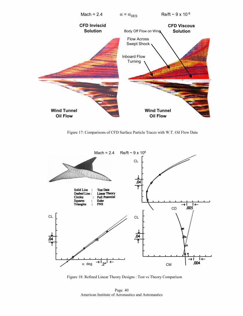
CL
Wind Tunnel Oil Flow
Wind Tunnel Oil Flow
CFD Inviscid Solution
CFD Viscous Solution
Inboard Flow Turning
Flow Across Swept Shock
Body Off Flow on Wing
Mach = 2.4 α = α DES Re/ft ~ 9 x 10 6
Figure 17: Comparisons of CFD Surface Particle Traces with W.T. Oil Flow DataPage 40 American Institute of Aeronautics and Astronautics
α deg CM
CL
CL
CD
Mach = 2.4 Re/ft ~ 9 x 10⁶
Figure 18: Refined Linear Theory Designs : Test vs Theory Comparison
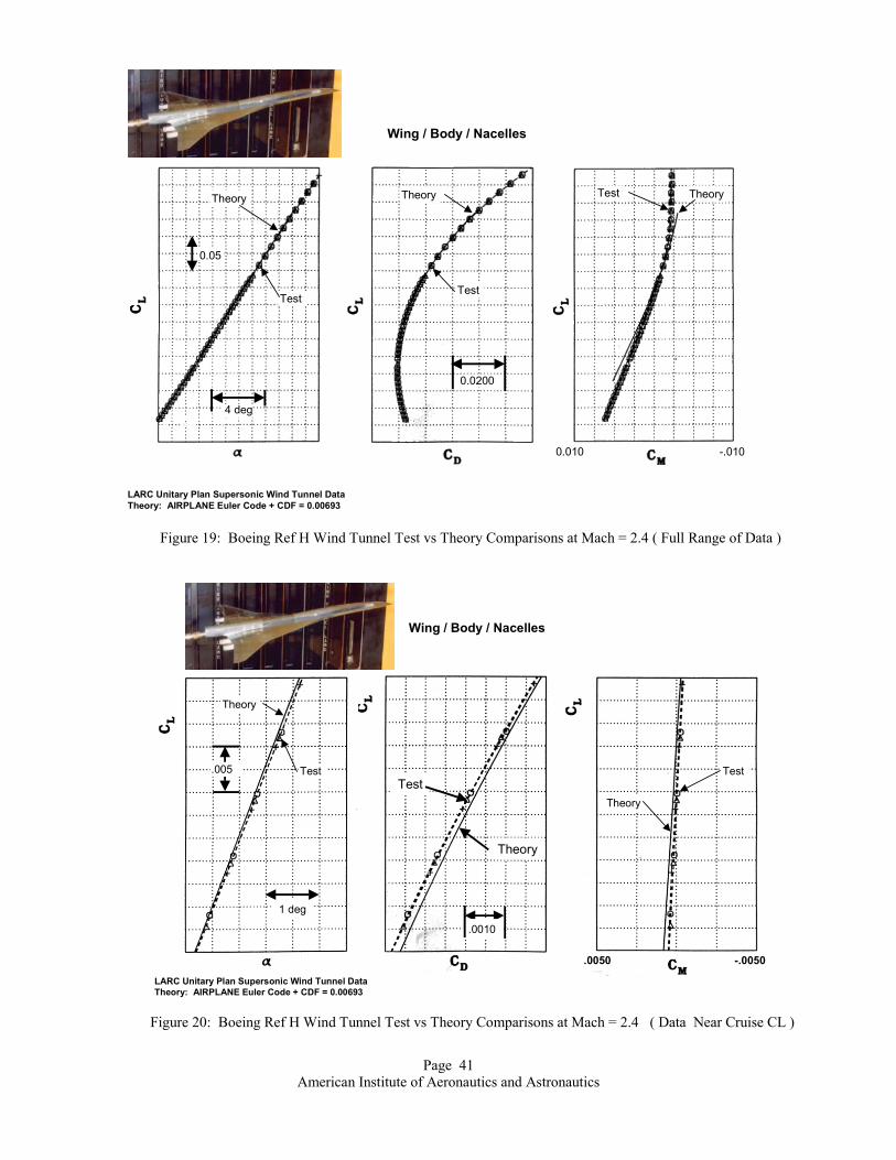
Wing / Body / Nacelles
LARC Unitary Plan Supersonic Wind Tunnel DataTheory: AIRPLANE Euler Code + CDF = 0.00693
Theory
Test
.0010
.0050 -.0050
1 deg
.005
Theory
Test
Theory
Test
LARC Unitary Plan Supersonic Wind Tunnel DataTheory: AIRPLANE Euler Code + CDF = 0.00693
Wing / Body / Nacelles
0.010 -.010
0.0200
4 deg
0.05
Theory
Test
Theory
Test
Test Theory
Figure 19: Boeing Ref H Wind Tunnel Test vs Theory Comparisons at Mach = 2.4 ( Full Range of Data )
Figure 20: Boeing Ref H Wind Tunnel Test vs Theory Comparisons at Mach = 2.4 ( Data Near Cruise CL )Page 41 American Institute of Aeronautics and Astronautics

Navie
CFL3D Euler and Navier-StokesBaldwin-Lomax Turbulence DataMach = 2.4 REC = 6.36x10⁶
α = 3.5O
Figure 21: Wing / Body Pressure Distributions Comparisons
-.00012
-.00003
Near Zero Lift Near Cruise
CL ~ 0.01
CL ~ 0.10
0.0002 Ref.
Ref.
-.00003
-.00020
ReC6.4 x 106
212 x 106
Euler
r Stokes Results (CFL3D) Predictions for Mach = 2.4
Figure 22: Effect of Reynolds Number on Wing / Body Pressure Drag
Page 42 American Institute of Aeronautics and Astronautics
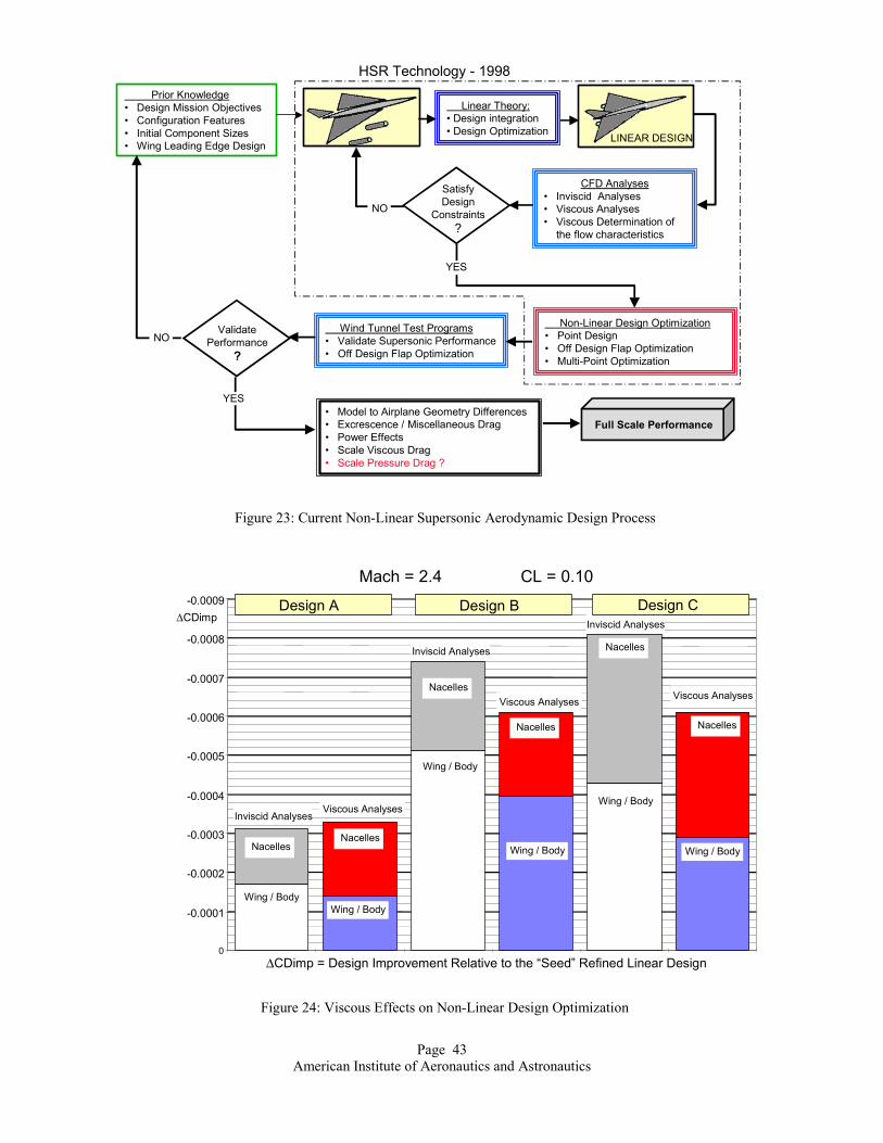
0
-0.0001
-0.0002
-0.0003
-0.0004
-0.0005
-0.0006
-0.0007
-0.0008
-0.0009∆CDimp
Prior Knowledge • Design Mission Objectives• Configuration Features• Initial Component Sizes• Wing Leading Edge Design
Linear Theory: • Design integration• Design Optimization
CFD Analyses• Inviscid Analyses• Viscous Analyses• Viscous Determination of
the flow characteristics
Wind Tunnel Test Programs • Validate Supersonic Performance• Off Design Flap Optimization
LINEAR DESIGN
ValidatePerformance
?
NO
SatisfyDesign
Constraints?
NONon-Linear Design Optimization
• Point Design• Off Design Flap Optimization• Multi-Point Optimization
YES
YES
Full Scale Performance• Model to Airplane Geometry Differences• Excrescence / Miscellaneous Drag• Power Effects• Scale Viscous Drag • Scale Pressure Drag ?
HSR Technology - 1998
Figure 23: Current Non-Linear Supersonic Aerodynamic Design Process
Page 43 American Institute of Aeronautics and Astronautics
Nacelles Wing / Body
Inviscid AnalysesViscous Analyses
Design A Design B
Inviscid Analyses
Viscous Analyses Viscous Analyses
Nacelles
Nacelles
Nacelles
Wing / Body
Wing / BodyWing / Body
Wing / Body
Wing / Body
∆CDimp = Design Improvement Relative to the “Seed” Refined Linear Design
Inviscid Analyses
Design C
Nacelles
Nacelles
Mach = 2.4 CL = 0.10
Figure 24: Viscous Effects on Non-Linear Design Optimization

62
61
60
59
58
57
56
55
CD
Vx
104
10 x 106 30 x 106 80 x 106
Reynolds Number
TLNS3D Pressure Drag Predictions
10 x 106 30 x 106 80 x 106
Reynolds Number
Test – TLNS3D Pressure DragTLNS3D Viscous DragFlat Plate Friction Drag
Viscous Drag Comparisons
0.0002
0.0002
CDP CDV
2.2% Ref H Wind Tunnel Model Mach = 0.9 CL = 0.18
Figure 25: Effect Of Reynolds Number on Wing/Body Pressure DragPage 44 American Institute of Aeronautics and Astronautics
CFD Code
VISCOUS CFD ANALYSES4 Boeing LBPW - CFL3D
(Bladwin / Lomax)5 NASA AMES - OVERFLOW
(Spaalart / Allmaras)6 Boeing Seattle - OVERFLOW
(Spaalart / Allmaras)7 NASA Ames - UPS
( Baldwin - Lomax)
1 2 3 4 5 6 7
Mach = 2.4 CL = 0.1 REL = 6.36 x10⁶
57.5
61.1
57.9 57.9
55.8 56.457.0
FLAT PLATE SKIN FRICTION1 NASA AMES - Nicolai2 Boeing LBPW - Van Driest3 Boeing Seattle - Sommer / Short
Typical HSCT Wing / Body
Figure 26: Comparisons of Fully Turbulent Flow Viscous Drag Predictions

Page 45 American Institute of Aeronautics and Astronautics
5
0
-5
-10
-15
-20
SpalartAllmaras
Test minus Theory Increment αααα ~ 5 deg
∆∆ ∆∆CD
x 1
04Rivers, and Wahls19
Mach = 0.90Rec = 30x106
BaldwinBarth
BaldwinLomax
Menter’sSST
5
0
-5
-10
-15
-20
Mach = 0.90 Rec = 30x106 Test minus Theory Increment α ~ 5 deg
∆CD x 104
Baldwin-BarthBaldwin-LomaxSpalart-AllmarasMenters SST
Figure 27: Test vs Theory Drag Comparison Including CFD Viscous Drag
Figure 28: Test vs Theory Drag Comparison Including Flat Plate Skin Friction Drag

Cf
106 107 108 109Rex
Theory: Modified Schultz / Grunow Test Data: Kulfan, R. M., D6-7161
.0050
.0045
.0040
.0035
.0030
.0025
.0020
.0015.
.0010
.0005
.0000
(Cfi)eq.0050
.0045
.0040
.0035
.0030
.0025
.0020
.0015
.0010
.0005
.0000 106 107 108
Equivalent Incompressible Reynolds Number
• (Cfi)eq = (T*/T) x Cf• (Rex)eq = (Rex) x (T/T* µ/µ*)
Mach 1.70 Matting, F. W., et alMach 2.00 Shutts, W. H., et alMach 2.15 Shutts, W.H., et alMach 2.25 Shutts, W.H., et alMach 2.50 Shutts, W.H.; Coles, D.Mach 2.95 Matting, F. W., et al+X
X
Cfi Mean
+σ
-σ
• The Mean Error Between Modified T* Skin Friction Equations and the Experimental Skin Friction Data measurements ~ 0.0 %
• Incompressible Experimental Cf Data: 1 σσσσ = +/- 2.7%
• Supersonic Experimental Cf Data: 1 σσσσ = +/- 3.8%
• Comparison with Modified Cf equations ~ Comparison withMean of the Test data.
Rex Eq
1 1060
2
4
6
8
10
12
14
16
18
20
22
24
26
28
30
32
34
36
38
40
Flat PlatFlat PlatFlat PlatCFD: CCFD: CCFD: CCFD: C
Loca
l Ski
n Fr
ictio
n , C
f -- c
ount
s
Figure 29: Flat Plate Local Skin Friction Database
Page 46 American Institute of Aeronautics and Astronautics
BCA OVERFLOW Local Skin friction Calculations Comparisons with Flat Plate Cf Spalart - Allmaras Turbulence Model Unform vertical grid spacing
1 106 1 107 1 108 1 10987
65
43
2
10
12
34
5
6Difference in Cf predictions -- Counts
Reynolds Number
Cf,c
fd -
Cf,f
p --
- C
ount
s
0.0
1 107 1 108 1 109
e Cf for Mach = 0.0e Cf for Mach 0.9e Cf for Mach = 2.4f for Mach = 0.9 Rel = 164 * 10^6f for Mach = 0.9 Rel= 6.044 * 10^6f for Mach = 2.4 Rel = 197 * 10^6f for Mach = 2.4 Rel = 6.362 * 10^6
Local Skin Friction Calculations
Reynolds Number, Rex
1 106 1 107 1 108 1 1091413121110987654321
0123456
Difference in Cf predictions -- Percent
Reynolds Number
(Cf,c
fd -
Cf,f
p)/C
f,fp
--- P
erce
nt
0.0
flight
wind tunnelWind Tunnel Reynolds Number
Flight Reynolds Number
Figure 30: Typical Evaluation of CFD Flat Plate Viscous Drag Prediction

Page 47 American Institute of Aeronautics and Astronautics
∆CDF = CDF x ∆CF/CF • HSCT Complete Configuration• Full Scale Reynolds Number ~Rel = 180 x106
∆CD
F =
CD
F x
∆CF/
CF
x 10
4 ~
coun
ts
Mach = 0.90 Mach = 2.40
εεεε = -0.98
εεεε = 1.66
-2.6 to 1.5
-0.7 to 3.1
4.0
3.0
2.0
1.0
0.0
-1.0
-2.0
-3.0
-4.0
The Differences in the Friction Drag Predictions at Full Scale Reynolds Numbers of ∆CD ~ 0.00038 is Equivalent to an an Uncertainty in the design MTOW of Nearly 40,000 lbs or would result in a Range Difference of 190 nmi for a Specific Design.
Baldwin - Lomax B - LSpalart Allmaras S - AMenter’s SST M SST
BPW BCA
CFL3D OVERFLOW
Differences in Percent
∆∆ ∆∆C
F/C
F =
(CF C
FD-C
F FP)
/CF F
P
x 10
2
L
8
6
4
2
0
- 2
- 4
- 6
- 8
-10
Mean
+1σσσσ
-1σσσσ
-1σσσσ
+1σσσσ
Mach ~ 0.0
Mach~ 0.5 to 3.0
TEST DATA
Mach = 0.5 , 0.9 Mach = 2.4, 2.5
Rel = 6.4 x 10⁶ (Wind Tunnel)Rel = 200 x 106 (Flight )
S
S
SS
S
A
LA
A
A
L
LL
L
L
BLB BCAG NASAAmes Turbulence Model
CFL3D OVERFLOW
L S A
Baldwin - LomaxSpalart - AllmarasMenter’s SST
Baldwin-Lomax
Baldwin-Lomax
Spalart-Allmaras
Spalart-Allmaras
Menter’sSST
Menter’sSST
S
• The Differences in the CFD Predictions of Skin Friction Greatly Exceed the Scatter in the Test Data.
Figure 32: Skin Friction Drag Prediction Errors at Full Scale Reynolds Numbers
Figure 31: CFD Flat Plate Viscous Drag vs Flat Plate Average Skin Friction Drag

Page 48 American Institute of Aeronautics and Astronautics
• ∆CDFW to F = ∆CDFFS -∆CDFWT • HSCT Complete Configuration• Reynolds Number Change ~Rel = 6.2 x 10⁶ to 180 x106
∆CD
F =
CD
F x
∆CF/
CF
x 10
4 ~
coun
ts
Baldwin - Lomax B - LSpalart Allmaras S - AMenter’s SST M SST
BPW BCA
Mach = 0.90 Mach = 2.40
εεεε = 3.50
εεεε = 1.24
0.7 to 4.9
-0.5 to 2.0
4.0
3.0
2.0
1.0
0.0
-1.0
-2.0
-3.0
-4.0
CFL3D OVERFLOW
Figure 33: Viscous Drag Prediction Errors - Wind Tunnel to Flight
Sommer / Short Fully Turbulent Sommer / Short Partly Laminar
∞ TTCF *
∞T T CF *
* * Re
T T x ∞ ∞
µ µ
** Re
T T x ∞ ∞
µ µ
Figure 34: Comparisons of Flat Plate Skin Friction Drag Predictions

Page 49 American Institute of Aeronautics and Astronautics
TU-144LL Flight Experiment InstrumentationNASA / Boeing /Tupolov HSR Research
Surface Pressure Taps and Skin-Friction Gages in Window Blanks
Experiment 3.3• 76 static pressures on
wing and fuselage• 16 skin friction gages• 3 boundary layer rakes
Experiment 1.2• 250 thermocouples
• 100 internal• 150 surface
XXXXXXX X X X X XXXXXXXX X X X XXXXXX X X XXXXX X XXXX X
X
XX
XXXX
XX
X
XX
X
X
Reference pressure probes
Alpha and Beta probes
Figure 35: TU-144LL Flight Experiment Instrumentation
Estimated Cf Uncertainty :+/- 2 to 4 Percent
Mach = 2.0 Re ~ 1.9 x 10⁶ /ft
Analyses by Paul Vijgen of Boeing
TU-144LL Flight Test Research Program
Figure 36: Flight Test Measurements of Local Skin Friction, Cf

Americ
M = 2.0 - WM = 2.0 -M = 0.5 - WM = 0.5 -
Figure 37: Concorde Flight Test - Skin Friction Data
M = 2.0 - WingM = 2.0 - BodyM = 0.5 - WingM = 0.5 - Body
ingBody
ingBody
Figure 38: Concorde Skin Friction - Computation and Flight Test Data Comparisons
Page 50 an Institute of Aeronautics and Astronautics

1 5432
Figure 39: YF-12A Flight Test Skin Friction Measurements
Page 51 American Institute of Aeronautics and Astronautics

106 107 108
Reynolds Number, Rex
0
1
23
4
5
67
8
9
10
Velo
city
Pro
file
"N" F
acto
r
u/Uo = (y/δδδδ)1/N
Empirical EquationSigalla, A.Kleebanoff, P. S., Diehl, Z. W.Smith, D. W., Walker, J.H.
Empirical EquationShutts, W.H., et al : Mach = 1.5 to 2.5Matting, F.W., et al : Mach = 2.95 to 4.2
( )NCfi
Cfi=
− ∗
max
. ( ),
.
.
0 1035 26
0 75
0 75
0
1
23
4
5
67
8
9
10
Velo
city
Pro
file
"N" F
acto
r
106 107 108
Reynolds Number, Rex
Figure 42: In
INCOMPRES
2.0
1.5
1.0
o.5
0.0
δ /x %
106
Test
Figure 41: Turbulent Boundary Layer Velocity Profile Shape Factor “N”
Page 52 American Institute of Aeronautics and Astronautics
compressible Turbulent Boundary Layer Thickness and Displacement Thickness
SIBLE BOUNDARY LAYER THICKNESS0.4
0.3
0.2
0.1
0.0
δ */x %
10 7 10 8Reynolds Number, Rex
106 10 7 10 8Reynolds Number, Rex
INCOMPRESSIBLE DISPLACEMENT THICKNESS
Theory
Test
Theory
Theory : Kulfan, B. M.Smith, D.W., and Walker, J.H. : Mach = 0.0 to 0.32

Page 53 American Institute of Aeronautics and Astronautics
106 107 108
Reynolds Number106 107 108
Reynolds Number
Boundary Layer Thicknessδδδδ / X x100
Boundary Layer Displacement Thicknessδδδδ* / X x100
Mach = 0.0Mach = 1.0Mach = 2.0Mach = 3.0
2.2
2.0
1.8
1.6
1.4
1.2
1.0
0.8
0.6
0.4
0.2
0.0
1.0
0.9
0.8
0.7
0.6
0.5
0.4
0.3
0.2
0.1
0.0
Theory: Kulfan, B.M.
Increasing Mach No.
Increasing Mach No.
TheoryMach = 1.7
TestM = 1.6 to 1.8
TheoryMach = 3.0 Theory
Mach = 0.0
TheoryMach = 2.0
TestM = 1.6 to 3.0
TestM = 0.0 to .32Test
M = 2.95
TestM = 2.0 to 2.2
TheoryMach = 3.0
2.42.22.01.81.61.41.21.00.80.60.40.20.0
2.42.22.01.81.61.41.21.00.80.60.40.20.0
δ/x %
δ/x %
δ/x %
δ/x %2.42.22.01.81.61.41.21.00.80.60.40.20.0
2.42.22.01.81.61.41.21.00.80.60.40.20.0
106 107 108Rex 106 107 108Rex
106 107 108Rex 106 107 108Rex
Shutts, W. H. et al
Matting, F. W. et al
Shutts, W. H. et al
Figure 43: Compressibility Effects on Boundary Layer Thickness
Figure 44: Compressibility Effects on Boundary Layer Thickness

Nacelle / Diverter Shocks
Intersecting Shocks
Fig
Figure 45: Impact of Favorable Nacelle - Airframe interference Drag
Page 54 American Institute of Aeronautics and Astronautics
Upper Limit of Boundary Layer
Upper Limit ofBack Flow in theBoundary Layer
A
B
ure 46: Reynolds Number Effects on Separation -- ?

Page 55 American Institute of Aeronautics and Astronautics
LaminarSeparation Turbulent
Separation
TransitionalRegion
Laminar Flow Turbulent Wake
TurbulentFlow
Turbulent Wake
Figure 47: Variation of Circular Cylinder Drag with Reynolds Number
Separation Surface
Open Two-Dimensional Separation Bubble Closed Two-Dimensional Separation Bubble
Upstream Limiting StreamlineDown Stream Limiting Streamline
S Singular Point
Separation Surface
Example of a Closed Two-Dimensional Separation BubbleLimiting Streamline
Figure 48: Two-Dimensional Flow Separation - Singular Separation

Page 56 American Institute of Aeronautics and Astronautics
S
P
P
P
Separation Line
Separation Bubble
Separation Line
P
P
Separation Surface
PP
P
Ordinary SeparationSeparation With an Isolated Singular Point
Upstream Limiting StreamlineDown Stream Limiting Streamline
S Singular PointP Ordinary Point
Figure 49: Three-Dimensional Separation
Top View of a 3D Closed Separation Bubble
Singular Attachment Point
Ordinary Separation Point
Ordinary Attachment PointSeparationSurface
Singular Separation Point
Figure 50: Examples of Separated Three Dimensional Flows With Reattachment
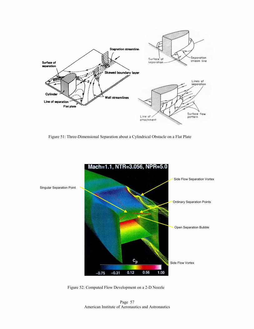
Figure 51: Three-Dimensional Separation about a Cylindrical Obstacle on a Flat Plate
Side Flow Separation Vortex
Open Separation Bubble
Ordinary Separation Points
Singular Separation Point
Side Flow Vortex
Figure 52: Computed Flow Development on a 2-D NozzlePage 57 American Institute of Aeronautics and Astronautics

Page 58 American Institute of Aeronautics and Astronautics
Incipient SeparationSeparated Flow
Attached Flow
Figure 53: Surface-Flow Pattern in a Swept-Shock / Boundary Layer Interaction - Ordinary Separation
View Along Shock View Along Shock
Separation Bubble
Vortical Slip Line
Attached Flow Separated Flow
Figure 54: Skin Friction Lines Beneath a Swept-Shock / Boundary Layer Interaction - Ordinary Separation

Compression CornerGlancing Shock Wave( Wedge on Flat Plate)
Incident Shock Wave
• Control Surface Deflections
• Wing Trailing Edge Shocks
• Vertical, Horizontal, Canard Trailing Edge Shocks
• Wing Inboard Compressions Coalescence Shock
• Body Compression Shocks
• Wing Apex / Body Junction
• Verticals on Wing Junctions
• Vertical or Horizontal tail / Body Junction
• Nacelle Boundary Layer Diverter
• 2D inlets Lip Shocks
• Axi-Symmetric Inlet Spike Shock
• Nacelle Shocks on Wing
• Shock Cancellation Concepts
• Adjacent Nacelles / Diverters
• Adjacent External Stores / Weapons
Crossing or Interfering Shocks
Figure 55: Fundamental Classes of Shock / Boundary Layer Interactions
Rex ~ 106 to 5 x10⁶
P1 P2
Flap Hinge Line Shocks
MN
Figure 56: Compression Corner Shock Separation CriteriaPage 59 American Institute of Aeronautics and Astronautics
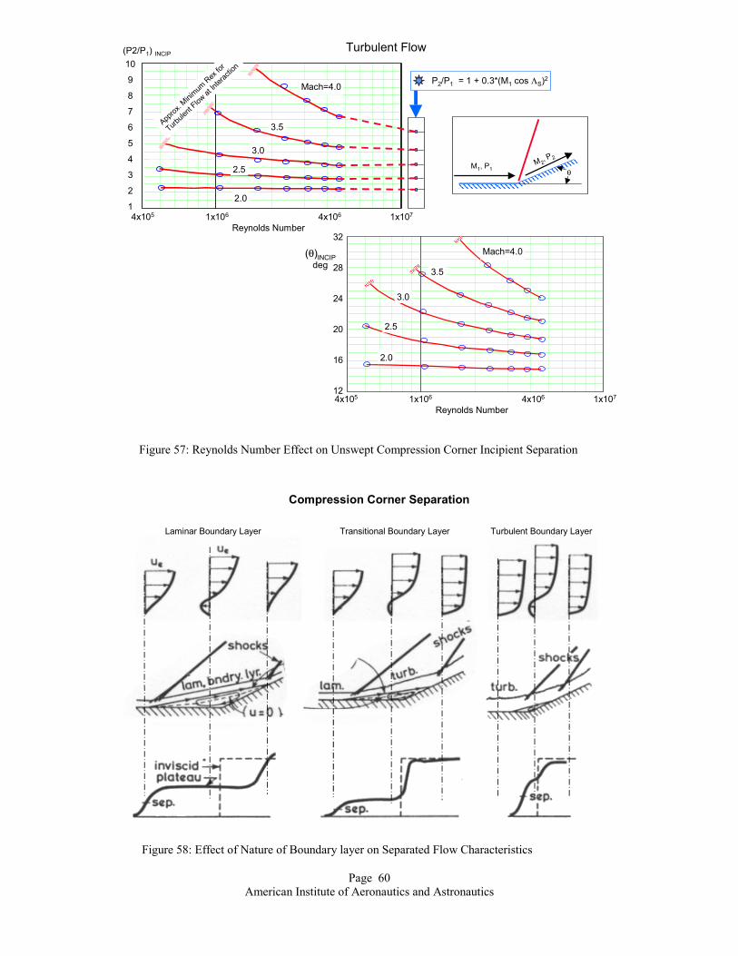
10
9
8
7
6
5
4
3
2
14x105 1x10⁶ 4x10⁶ 1x10⁷
Reynolds Number
P2/P1 = 1 + 0.3*(M1 cos ΛS)2
Approx
. Minim
um Rex
for
Turbule
nt Flow
at In
terac
tion
(P2/P1) INCIP
2.5
3.0
3.5
2.0
Mach=4.0
4x10⁵ 1x10⁶ 4x10⁶ 1x10⁷
Reynolds Number
32
28
24
20
16
12
M1, P1M 2, P2
θ
(θ)INCIPdeg
Turbulent Flow
2.5
3.0
3.5
2.0
Mach=4.0
Figure 57: Reynolds Number Effect on Unswept Compression Corner Incipient Separation
Laminar Boundary Layer Transitional Boundary Layer Turbulent Boundary Layer
Compression Corner Separation
Figure 58: Effect of Nature of Boundary layer on Separated Flow Characteristics
Page 60 American Institute of Aeronautics and Astronautics

Page 61 American Institute of Aeronautics and Astronautics
4.5
4.0
3.5
3.0
2.5
2.0
1.5
1.0
5.0
4.5
4.0
3.5
3.0
2.5
2.0
1.5
1.00 .5 1.0 1.5 2.0 2.5 3.0 3.5X/L
0 .25 .50 .75 1.00 1.25 1.5X/L
5.0
4.5
4.0
3.5
3.0
2.5
2.0
1.5
1.0.7 .8 .9 1.0 1.1 1.2 1.3 1.4
X/L
PPO
PPO
PPO
Pure Laminar SeparationMO = 3.0
Transitional SeparationMO = 2.7
Turbulent SeparationMO = 2.7
MO, PO
L
Separation Region
Increasing RexIncreasing Rex
Figure 59: Reynolds Number Effect on Separation Regions and Pressure Distributions
13
12
11
10
9
8
7105 106 107 108
Reynolds Number
Turbulent Flow
105 106 107 108
Reynolds Number
(P2/P1) INCIP7
6
5
4
3
2
M1, P1
M2, P2
φ
1 2 3 4Mach Number
7
6
5
4
3
2
(P2/P1) INCIP
Limiting Pressure Ratioφ = 7.5 degReflection Factor = 1.7
( )2
1
2 cos065.0313.2 sLOCMPP Λ+=
ShockDetachment
M1 = 3.853.40
2.93
2.60
M1 = 3.85
3.402.93
2.60
(φ)INCIP
Figure 60: Reynolds Number Effect on Unswept Incident Shocks Incipient Separation

Page 62 American Institute of Aeronautics and Astronautics
Separated Flow
Attached Flow
5.11
2 =PP
StanbrookMcCabeLowrie
Shoc
k De
tach
men
t
Flow Deflection Angle at Separation
1.0 1.5 2.0 2.5 3.0 3.5Mach Number
15
10
5
0
δSdeg
Curved Mid-Body
75O
Separated Flow Behind Strong Body Induced Shock
Theoretical Inviscid Shock
Observed Separation Line
Mach 3.0α = 0O
Figure 61: Example of Body Induced Glancing Shock Separation
Figure 62: Glancing Shock Wave / Boundary Layer Separation Criteria

1.01.21.41.61.82.02.22.42.62.83.03.23.43.63.84.0
1.0 1.2 1.4 1.6 1.8 2.0 2.2 2.4 2.6 2.8 3.0Mach Number
(P2/P1)INCIP
Glancing Shock
Unswept Compression Corner
Unswept Incident Shock
45O Swept Compression Corner
Shock Pressure
Rise∆Cp
.5
.4
.4
.4
.4
.3
.3
.3
.3
.2
.2
.2
.2
.1
.1
.1
.1
.0
.0
.0
.0
Figure 63: Comparison of Shock Separation Criteria – Turbulent Flow
Mach = 2.4
Glancing Shock Criteria
Contours are Lines of Constant Shock Strength, P2/P1
3.88
3.75
3.63
3.503.38 3.25 3.13 3.00
2.71
2.63 2.502.38
2.25
2.13
2.00
1.88
1.75
1.63
1.38
1.250
1.13
00755025007550250075502500755025007550250-.10 -.08 -.06 -.04 -.02 .00 .02 .04 .06 .08 .10
Pressure Upstream of the shock, Cp1
Separated Flow
Attached Flow
1.50
2.88
Incident Shock Criteria
45O Compression Shock Criteria
Figure 64: Amplification of Shock Pressure Rise by Local Pressure FieldPage 63 American Institute of Aeronautics and Astronautics

Page 64 American Institute of Aeronautics and Astronautics
Color Oil FlowFlorescent Oil Dots
Mach = 2.4 Test Results
CFD Calculated Results Double Wedge Experiment
Figure 65: Weak Crossing Shock Interactions
A
C
D
E
F
F
E
D
C
B
A
B
CFL3D Euler and Navier-StokesBaldwin-Lomax Turbulence ModelReC = 6.36 x 10⁶
Mach = 2.4 α = 3.5O
Figure 66: Test vs Theory Pressure Distributions for a Wing/Body/Nacelle/Diverter Configuration

A
C
D
E
F
F
E
D
C
B
A
B
CFL3D Euler and Navier-StokesBaldwin-Lomax Turbulence ModelMach = 2.4 α = 3.5O
Figure 67: Reynolds No. Effect on Wing/Body/Nacelle/Diverter Configuration Pressure Distributions
Page 65 American Institute of Aeronautics and Astronautics
Mach = 2.4
Glancing Shock
Separation Criteria
∆Cp
.300
.275
.250
.225
.200
.175
.150
.125
.100
.075
.050
.025
.00
Contours are Lines of Constant Shock Strength, P2/P1
2.00
-.08 -.06 -.04 -.02 .00 .02 .04 .06 .08Cp1
1.88
1.63
1.75
Separated Flow
Attached Flow
2.25 2.132.382.50
1.38
1.250
1.13
C
BA
DC
AA
D
C
BB
D
1.50
X
XX
Inviscid Shock StrengthViscous Shock Strength, ReC = 6.36 x 10⁶ at Station “X”Viscous Shock Strength, ReC = 212 x 106
Figure 68: Nacelle-on-Wing Shock Strength Comparisons
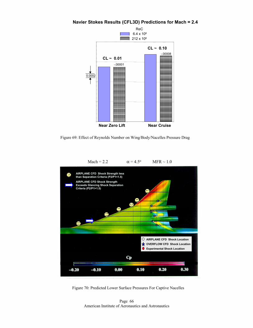
Page 66 American Institute of Aeronautics and Astronautics
ReC6.4 x 106
212 x 106
Navier Stokes Results (CFL3D) Predictions for Mach = 2.4
0.0002
-.00001
-.00008
Near Zero Lift Near Cruise
CL ~ 0.01
CL ~ 0.10
Figure 69: Effect of Reynolds Number on Wing/Body/Nacelles Pressure Drag
Mach = 2.2 α = 4.5o MFR ~ 1.0
AIRPLANE CFD Shock Strength less than Separation Criteria (P2/P1<1.5)
AIRPLANE CFD Shock Strength Exceeds Glancing Shock Separation Criteria (P2/P1>1.5)
AIRPLANE CFD Shock LocationOVERFLOW CFD Shock LocationExperimental Shock Location
Figure 70: Predicted Lower Surface Pressures For Captive Nacelles
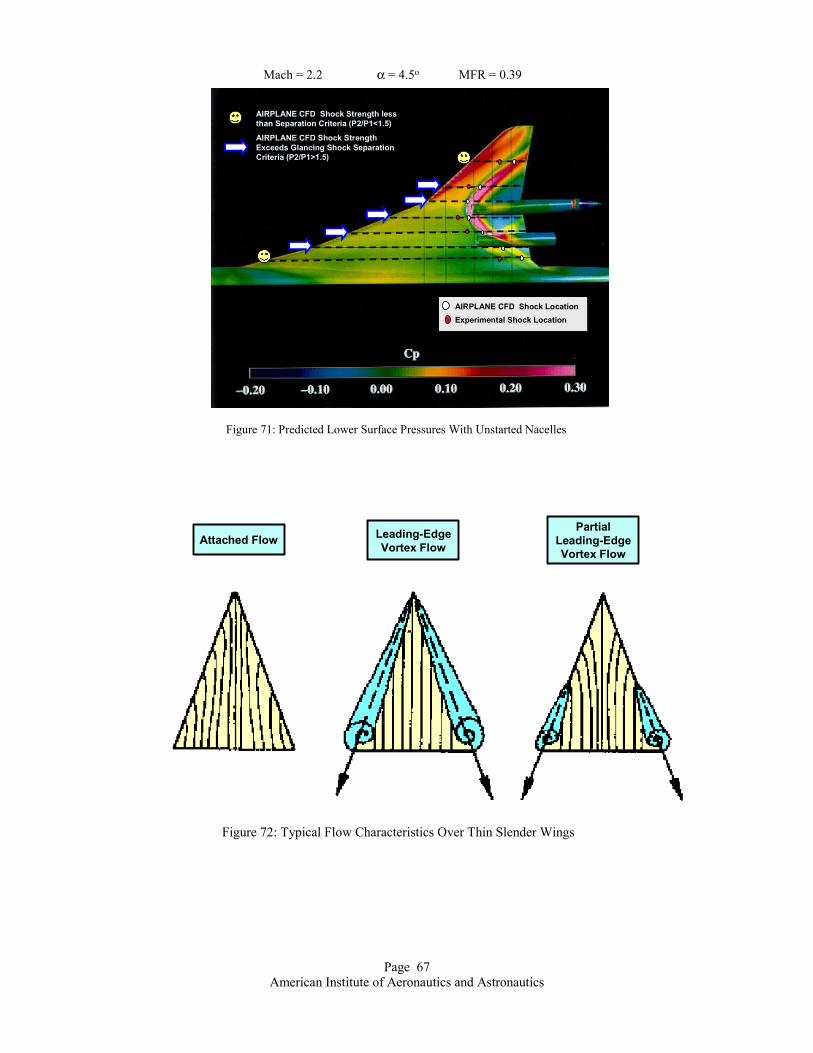
Atta
Mach = 2.2 α = 4.5o MFR = 0.39
AIRPLANE CFD Shock Strength less than Separation Criteria (P2/P1<1.5)
AIRPLANE CFD Shock Strength Exceeds Glancing Shock Separation Criteria (P2/P1>1.5)
AIRPLANE CFD Shock LocationExperimental Shock Location
Figure 71: Predicted Lower Surface Pressures With Unstarted Nacelles
ched Flow Leading-EdgeVortex Flow
PartialLeading-EdgeVortex Flow
Figure 72: Typical Flow Characteristics Over Thin Slender Wings
Page 67 American Institute of Aeronautics and Astronautics

Page 68 American Institute of Aeronautics and Astronautics
Experimental Vortex Flow Visualization
Figure 73: Leading Edge Vortex Flow on Highly Swept Wings
Figure 74: Wing Leading Edge Vortex Features

1.5
1.0
0.5
0.00 0.5 1.0
CL
∆CDCL2
1.5
1.0
0.5
0.00 0.5 1.0
CL
∆CDCL2
1.5
1.0
0.5
0.00 0.5 1.0
CL
∆CDCL2
Mach ~ 0
1πAR
Zero Suction(No Vortex Lift)
Suction Analogy
Test Data
76O70O80O
CLP
α, degrees
Theory
Test
CL CLCL
α, degrees α, degrees α, degrees
Theory
Theory
Theory
Test
Test
Test
CLP
CLP
CLV
MACH ~ 0.1
Figure 75: Leading Edge Suction Analogy Predictions - Thin, Sharp-Edge Wings
Figure 76: Suction Analogy Drag Due to Lift Predictions
Page 69 American Institute of Aeronautics and Astronautics
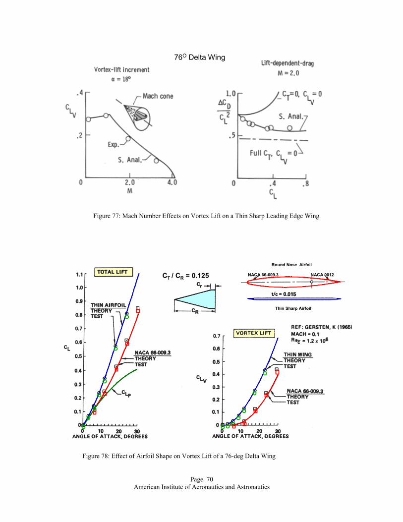
Page 70 American Institute of Aeronautics and Astronautics
76O Delta Wing
Figure 77: Mach Number Effects on Vortex Lift on a Thin Sharp Leading Edge Wing
NACA 66-009.3 NACA 0012
Thin Sharp Airfoil
Round Nose Airfoil
CT / CR = 0.125
Figure 78: Effect of Airfoil Shape on Vortex Lift of a 76-deg Delta Wing

• Mach = 0.85• Flat Symmetric Wing
71.2O
Predicted Start of Leading Edge Vortex @ Local Wing Station
Pressure Break
∆CpL Before Pressure Break∆CpL After Break
Typical Pressure Measurement Across The Span
at 2.5% Local Chord
∆CpL = CpLOWER – CpUPPER at Same Station
Figure 79: Comparison of Predicted and Measured Formation Vortex Boundaries
71.2O
Vary δF Across Span
Figure 80: Effect of Flap Deflections on Leading Edge Vortex DevelopmentPage 71 American Institute of Aeronautics and Astronautics

Page 72 American Institute of Aeronautics and Astronautics
Outboard Vortex WithNo Flap Deflection
Attached Flow WithOutboard Flap Deflection
Mach ~ 0.90
Figure 81: Effect of Flap Deflections on Surface Streamlines
-0.5
-0.4
-0.3
-0.2
-0.1
0.0
0.1
0.2
0.3
0.4
0.5
-8 -7 -6 -5 -4 -3 -2 -1 0 1 2 3 4 5 6 7 8
0.090.200.350.500.650.800.93
2y/b
α deg
∆CpL @ 2.5% Chord
-8
-6
-4
-2
0
2
4
6
8
0.0 0.1 0.2 0.3 0.4 0.5 0.6 0.7 0.8 0.9 1.02y/b
α deg
Attached Flow
Separated Flow
Figure 82: Leading Edge Vortex Development on an Arrow Wing At Mach = 1.7

Page 73 American Institute of Aeronautics and Astronautics
-8
-6
-4
-2
0
2
4
6
8
0.0 0.1 0.2 0.3 0.4 0.5 0.6 0.7 0.8 0.9 1.0
Attached Flow
Separated Flow
2y/b
α deg
-0.5
-0.4
-0.3
-0.2
-0.1
0.0
0.1
0.2
0.3
0.4
0.5
-8 -7 -6 -5 -4 -3 -2 -1 0 1 2 3 4 5 6 7 8
0.090.200.350.500.650.800.93
2y/b
∆CpL @ 2.5% Chord
α deg
Figure 83: Leading Edge Vortex Development on an Arrow Wing At Mach = 2.1
Sharp Leading EdgeMach = 0.83Re = 6x10⁶
0 2 4 6 8 10 12 14 16Angle of Attack deg
1.6
1.4
1.2
1.0
0.8
0.6
0.4
0.2
0.0
∆CP
∆CP @ 2y/b = 0.975
0.2 0.3 0.4 0.5 0.6 0.7 0.8 0.9 1.0Streamwise Station X/CR
14
12
10
8
6
4
2
0
α deg
X/CR = 0.60
X/CR = 0.95
X/CR = 0.80
X/CR = 0.40 Attached Flow
Vortex Flow
• Sharp Leading Edge• Small Radius• Medium Radius• Large Radius
Not to Scale
Figure 84: Spanwise Movement of the Leading Edge Vortex With Angle of Attack

Medium Round Leading EdgeMach = 0.85Re = 6x10⁶
0 2 4 6 8 10 12 14 16Angle of Attack deg
1.6
1.4
1.2
1.0
0.8
0.6
0.4
0.2
0.0
∆CP
∆CP @ 2y/b = 0.975
0.2 0.3 0.4 0.5 0.6 0.7 0.8 0.9 1.0Streamwise Station X/CR
14
12
10
8
6
4
2
0
α deg
Attached Flow
Vortex FlowX/CR = 0.60
X/CR = 0.95
X/CR = 0.80
X/CR = 0.40
Figure 85: Spanwise Movement of the Leading Edge Vortex With Angle of Attack
Mach ~ 0.83 to 0.85
Airfoil Closure Region
14
12
10
8
6
4
2
0
α deg
Stream Wise Station X/CR0.2 0.3 0.4 0.5 0.6 0.7 0.8 0.9 1.0
Attached Flow
Vortex FlowAttached Flow
Vortex Flow
Medium Round Leading Edge
Sharp Leading Edge
Figure 86: Leading Edge Radius Effect on Inboard Movement of the Leading Edge VortexPage 74 American Institute of Aeronautics and Astronautics

Page 75 American Institute of Aeronautics and Astronautics
0 2 4 6 8 10 12 14 16Angle of Attack deg
1.6
1.4
1.2
1.0
0.8
0.6
0.4
0.2
0.0
∆CP
0.2 0.3 0.4 0.5 0.6 0.7 0.8 0.9 1.0Streamwise Station X/CR
14
12
10
8
6
4
2
0
α deg
∆CP @ 2y/b = 0.975
X/CR = 0.95
X/CR = 0.80
X/CR = 0.60
X/CR = 0.40
Medium Round Leading EdgeMach = 0.85Re = 24x106
Attached Flow
Vortex Flow
Figure 87: Spanwise Movement of the Leading Edge Vortex With Angle of Attack for Re = 24 x 106
0 2 4 6 8 10 12 14 16Angle of Attack deg
1.6
1.4
1.2
1.0
0.8
0.6
0.4
0.2
0.0
∆CP
∆CP @ 2y/b = 0.975
X/CR = 0.95
X/CR = 0.80
X/CR = 0.60
X/CR = 0.40
Medium Round Leading EdgeMach = 0.85Re = 48x106
0.2 0.3 0.4 0.5 0.6 0.7 0.8 0.9 1.0Streamwise Station X/CR
14
12
10
8
6
4
2
0
α deg
Attached Flow
Vortex Flow
Figure 88: Spanwise Movement of the Leading Edge Vortex With Angle of Attack for Re = 48 x 106

0 2 4 6 8 10 12 14 16Angle of Attack deg
1.6
1.4
1.2
1.0
0.8
0.6
0.4
0.2
0.0
∆CP
Medium Round Leading EdgeMach = 0.85Re =96x106
∆CP @ 2y/b = 0.975
X/CR = 0.95
X/CR = 0.80
X/CR = 0.60
X/CR = 0.40
0.2 0.3 0.4 0.5 0.6 0.7 0.8 0.9 1.0Stream Wise Station X/CR
14
12
10
8
6
4
2
0
α deg
Attached Flow
Vortex Flow
Figure 89: Spanwise Movement of the Leading Edge Vortex With Angle of Attack for Re = 96 x 106
0 2 4 6 8 10 12 14 16Angle of Attack deg
1.6
1.4
1.2
1.0
0.8
0.6
0.4
0.2
0.0
∆CP
Medium Round Leading EdgeMach = 0.85Re =120x106
∆CP @ 2y/b = 0.975
X/CR = 0.95
X/CR = 0.80
X/CR = 0.60
X/CR = 0.40
0.2 0.3 0.4 0.5 0.6 0.7 0.8 0.9 1.0Stream Wise Station X/CR
14
12
10
8
6
4
2
0
α deg
Attached Flow
Vortex Flow
Figure 90: Spanwise Movement of the Leading Edge Vortex With Angle of Attack for Re = 120 x 106Page 76 American Institute of Aeronautics and Astronautics

Page 77 American Institute of Aeronautics and Astronautics
Medium Round Leading EdgeMach = 0.85
14
12
10
8
6
4
2
0
α deg
24 x 106 and 48 x 106
6 x 10⁶ , 96 x 106 and 120 x 106
Airfoil Closure Region
Stream Wise Station X/CR0.2 0.3 0.4 0.5 0.6 0.7 0.8 0.9 1.0
Vortex Flow
Attached Flow
Figure 91: Reynolds Number Effect on Inboard Movement of the Leading Edge Vortex
0 4 8 12 16 20 24 28Angle of Attack deg
Angle of Attack deg 0 4 8 12 16 20 24 28
1.4
1.2
1.0
0.8
0.6
0.4
0.2
0.0
CL.10
.05
0.0
-.05
-.10
-.15
-.20
-.25
-.30
-.35
-.40
CM
Medium Round Leading EdgeMach = 0.85Re = 6x10⁶ to 120 x 106
Figure 92: Effect of Reynolds Number on Lift and Pitching Moment for a 65O Delta Wing

Page 78 American Institute of Aeronautics and Astronautics
Figure 93: Two-Dimensional Crossflow Plane Potential Flow Analyses Methods
Thin Sharp Edge Highly Swept Wings
Figure 94: Three Dimensional Potential Flow Analysis Models of Leading Edge Vortex Flow
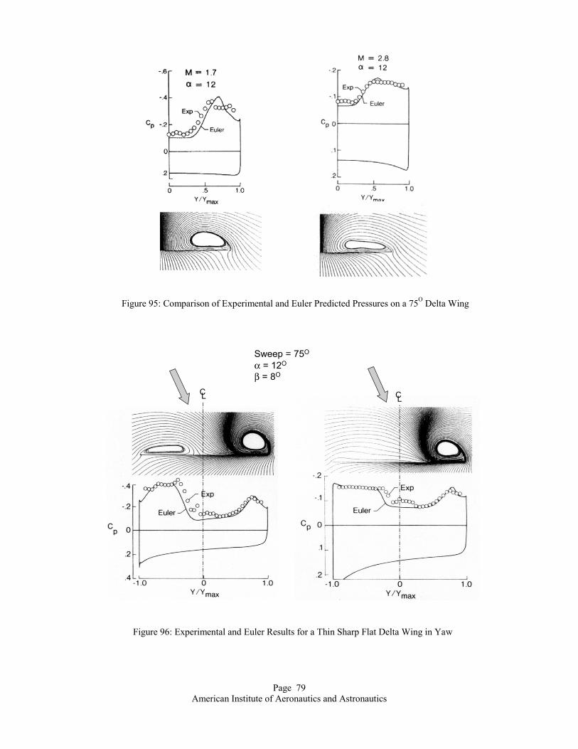
Figure 95: Comparison of Experimental and Euler Predicted Pressures on a 75O Delta Wing
Page 79 American Institute of Aeronautics and Astronautics
CL CL
Sweep = 75O
α = 12O
β = 8O
Figure 96: Experimental and Euler Results for a Thin Sharp Flat Delta Wing in Yaw

Page 80 American Institute of Aeronautics and Astronautics
65o Cropped Delta Wing Mach Mach = 0.85 α = 10o
EULER SOLUTION NAVIER STOKES SOLUTION
Pathlines
Wing Isobars
Total Pressure ContoursX/Cr = 0.8
Vorticity ContoursX/Cr = 0.8
∆CP = 0.1
∆CPT = 0.05
∆| rot v | = 0.0001
Origin of Leading Edge Vortex
Origin of Leading Edge Vortex
Primary Vortex Primary Vortex
Secondary Vortex Secondary Vortex
Figure 97: Comparisons of Euler and Navier-Stokes Solution
65o Cropped Delta Wing Mach = 0.85
Rec = 1.28 x 10⁶ α = 10O
0.0 0.2 0.4 0.6 0.8 1.0η = y/s
-1.6
-1.2
-0.8
-0.4
0.0
0.4
CP
0.0 0.2 0.4 0.6 0.8 1.0η = y/s
-1.6
-1.2
-0.8
-0.4
0.0
0.4
CP
0.0 0.2 0.4 0.6 0.8 1.0η = y/s
-1.6
-1.2
-0.8
-0.4
0.0
0.4
CP X/CR = 0.3
X/CR = 0.6 X/CR = 0.8
65O
λ = 0.15
Round Nose Airfoil:T/C mac = 5 %LE radius = 0.7%
Test DataNavier-StokesEuler
Figure 98: Comparisons of Euler and Navier-Stokes Laminar Flow Results

Page 81 American Institute of Aeronautics and Astronautics
CFL3D Spalart-Allmaras Turbulence Model Round Leading Edge
65O
α = 16.37O Rn = 6 x 10⁶ α = 16.44O Rn = 48 x 106
α = 16.38O Rn = 84 x 106 α = 16.59O Rn = 120 x 106
A
A
Primary Leading Edge Vortex
Secondary Vortex
Trailing Edge Separation
Figure 99: Effect of Reynolds Number on Computed Surface Streamlines Mach = 0.85
CFL3D Turbulent Flow AnalysesMach = 0.85 Rn = 6x10⁶
Round Leading Edge Geometry
Attached Flow Condition α = 7.14O
Separated Flow Condition α = 12.28O
Figure 100: Comparison of Predicted and Measured Spanwise Pressure Distributions

Page 82 American Institute of Aeronautics and Astronautics
CFL3D Predictions Wind Tunnel Data
65O Flat Delta Wing With Round Leading EdgeMach = 0.85 α ~ 12O
CFL3D Predictions Wind Tunnel Data
65O Flat Delta Wing With Round Leading EdgeMach = 0.85 α ~ 7O
Figure 101: Comparisons of Predicted Reynolds Number Effects on Cp with Test Data: α = 7O
Figure 102: Comparisons of Predicted Reynolds Number Effects on Cp with Test Data: α = 12O

Page 83 American Institute of Aeronautics and Astronautics
-.40
-.35
-.30
-.25
-.20
-.15
-.10
-.05
.000 .1 .2 .3 .4 .5 .6 .7 .8 .9 1.
Semi Span Station η = 2y/b
CP
-.40
-.35
-.30
-.25
-.20
-.15
-.10
-.05
.000 .1 .2 .3 .4 .5 .6 .7 .8 .9 1.
Semi Span Station η = 2y/b
CP
(Blunt)
• CFL3D Results• 65O Flat Delta Wing• Mach = 1.60• Re = 106
• Turbulent Flow Model
α = 4 deg α = 8 deg
Figure 103: The Effect of Leading Edge Radius on Upper Surface Pressures
Effect of Camber -Turbulent Flow Model-.50
-.45
-.40
-.35
-.30
-.25
-.20
-.15
-.10
-.05
.000 .1 .2 .3 .4 .5 .6 .7 .8 .9 1.
Semi Span Station η = 2y/b
CP
αC = 10.0O
αC = 8.0O
αC = 4.0O
αC = 0.0O
CFL3D Results65O Flat Delta WingMach = 1.60α = 8 degRe = 106
Camber Variations – Medium nose Radius ( 20:1 Ellipse)
Figure 104: The Effect of Leading Edge Camber on Upper Surface Pressures

Page 84 American Institute of Aeronautics and Astronautics
Re = 1.0 x 10⁶
Re = 2.0 x 10⁶
Re = 5.0 x 10⁶
-.45
-.40
-.35
-.30
-.25
-.20
-.15
-.10
-.05
.000 .1 .2 .3 .4 .5 .6 .7 .8 .9 1.
Semi Span Station η = 2y/b
CP
Uncambered Elliptic Nose airfoil
0 .1 .2 .3 .4 .5 .6 .7 .8 .9 1.
Semi Span Station η = 2y/b
-.50
-.45
-.40
-.35
-.30
-.25
-.20
-.15
-.10
-.05
.00
CP
Cambered Elliptic Nose airfoil αC = 10O
CFL3D Results65O Flat Delta WingMach = 1.60α = 8 degTurbulent Flow Model
Figure 105: The Effect of Reynolds Number on Upper Surface Pressures
αC = 10.0O-.50
-.45
-.40
-.35
-.30
-.25
-.20
-.15
-.10
-.05
.000 .1 .2 .3 .4 .5 .6 .7 .8 .9 1.
Semi Span Station η = 2y/b
CP
Laminar Flow Model
Turbulent Flow Model
CFL3D Results65O Flat Delta WingMedium Leading Edge RadiusMach = 1.60α = 8 degRe = 106
Figure 106: The Effect of Laminar Flow Versus Turbulent Flow on Upper Surface Pressures

Page 85 American Institute of Aeronautics and Astronautics
Turbulent FlowLaminar Flow
ARC3D 75O Flat Delta WingSharp Thin Leading EdgeMach = 1.95α = 20 degRe = 4.48 x 10⁶
Figure 107: The Effect of Laminar Flow Versus Turbulent Flow on Upper Surface Pressures
ΛLE
0.0 -.01 -.02 -.03 -.04 -.05CM
1.0
0.9
0.8
0.7
0.6
0.5
0.4
0.3
0.2
0.1
0.0
CL
.01 0.0 -.02 -.04 -.06CM
1.0
0.9
0.8
0.7
0.6
0.5
0.4
0.3
0.2
0.1
0.0
CL50O
60O
70O
• Subsonic Speeds• Wind Tunnel Reynolds Number
ΛLE = 75O
Figure 108: Planform Effects on Pitching Moment

Page 86 American Institute of Aeronautics and Astronautics
12O Angle of Attack
F-16
YF-17
-5.0 0.0 5.0 10.0 15.0 20.0 25.0 30.0Angle of Attack deg
2.0
1.8
1.6
1.4
1.2
1.0
0.8
0.6
0.4
0.2
0.0
-.2
-.4
CL
α = 18O
α = 0O
α = 0O
α = 6O
α = 6O
α = 12O
α = 18O
α = 12O
Mach ~ 0.1
Figure 109: Wing Strake Effects on Lift and Wing Flow Characteristics
Figure 110: Comparison of Wind Tunnel and Flight Observed Flow Development

Page 87 American Institute of Aeronautics and Astronautics
Figure 111: Effect of Mach Number on Lift and Pitching Moment
Mach = 1.2αααα ~ 11O
Mach = 1.2αααα ~ 11O
Mach = 0.8αααα ~ 11O
Figure 112: Effect of Mach Number on Flow Patterns, αM = 10 deg.

Page 88 American Institute of Aeronautics and Astronautics
αααα = 12O
Experimental Oil Flow Pattern
Computed Surface Stream lies
Computed Off-Surface Particle Traces
Computed Total Pressure Contours
80O
40O
ΛLE = 50O ΛLE = 60O
ΛLE = 70O
ΛLE = 75O
0.5 1.0 1.5 2.0 2.5 3.0 3.5Mach Number
20
15
10
5
0
α deg
Attached Flow
LE VortexFlow
Figure 113: Effect of Mach Number on Wing / Strake Flow Patterns, ΛLE = 70 deg.
Figure 114: Flow Characteristics Over a Round-Edge Double Delta Wing

-2.0
-1.0
0.0
1.00 .25 .50
Semi-Span S
CP
-2.0
-1.0
0.0
1.00 .25 .50
Semi-Span Sta
CP
α = 12O
α = 25O
Computed Total Pressure Contours
α = 6O
α = 20Oα = 15O
α = 12O
α = 30O
α = 25O
α = 40Oα = 35O
Figure 115: Effect of Angle of Attack on Vortex Growth
0 10 20 30 40 50Angle of Attack deg.
1.4
1.2
1.0
0.8
0.6
0.4
0.2
0.0
Theory
Test
CL
.75 1.0tation η
.75 1.0tion η
-2.0
-1.0
0.0
1.00 .25 .50 .75 1.0
Semi-Span Station η
CP
-2.0
-1.0
0.0
1.00 .25 .50 .75 1.0
Semi-Span Station η
CP
Pressure Distribution at X/CR = 0.75
α = 15O
α = 30OTheory
Test
• Navier-Stokes (Laminar)• Mach = 0.0• Rel = 1.3 x 10⁶
VortexBursting
Figure 116: Spanwise Pressure Distributions and Total Lift CoefficientPage 89 American Institute of Aeronautics and Astronautics

Page 90 American Institute of Aeronautics and Astronautics
Wing/Body/Nacelles Flaps up
Wing/Body/Nacelles Outboard Flaps deflected δLE/δTE = 10O/3O
Mach = 0.90Round Nose Airfoils
Sharp Nose Airfoils
Attached Flow
Attached Flow
UpperSurface
LE Vortex
UpperSurface
LE Vortex
LowerSurface
LE Vortex
LowerSurface
LE Vortex
Figure 117: HSCT Wing Leading-Edge Pressure Characteristics
107 4x10⁷ 108
Reynolds Number
CD.0085.0080.0075.0070.0065.0060.0055.0050
CM.0145.0140.0135.0130
107 4x10⁷ 108
Reynolds Number
Wing / Body / Nacelles - Flaps Up Mach = 0.90Min. Drag Condition
α= 1.1 degTransonic Cruise Condition
α= 5.0 deg
CF Extrapolation
107 4x10⁷ 108
Reynolds Number
CM.0090.0085.0080.0075
CM.0095.0085.0075.0065.0055.0045.0035
107 4x10⁷ 108
Reynolds Number
107 4x10⁷ 108
Reynolds Number
CD.0195.0190.0185.0180.0175.0170.0165.0160
107 4x10⁷ 108
Reynolds Number
CD.0605.0600.0595.0590.0585.0580.0575
107 4x10⁷ 108
Reynolds Number
CL.010.005
.0-.005
107 4x10⁷ 108
Reynolds Number
CL.225.220.215.210
107 4x10⁷ 108
Reynolds Number
CL.450.445.440.435.430
High Angle of Attack Condition
α= 9.0 deg
1%
δH ~ 0.1O
Figure 118: Longitudinal Coefficients Trends With Reynolds Number - Flaps Up

CM.0045.0040.0035.0030
107 4x10⁷ 108
Reynolds Number
Wing / Body / Nacelles - Flaps Deflected Mach = 0.90Min. Drag Condition
α= 1.1 degTransonic Cruise Condition
α= 5.0 deg
CF Extrapolation
107 4x10⁷ 108
Reynolds Number
CM-.0005-.0010-.0015-.0020-.0025
CM-.0010-.0015-.0020-.0025-.0030-.0035-.0040
107 4x10⁷ 108
Reynolds Number
107 4x10⁷ 108
Reynolds Number
CD.0100.0095.0090.0085.0080.0075.0070.0065
107 4x10⁷ 108
Reynolds Number
CD.0180.0175.0170.0165.0160.0155.0150.0145
107 4x10⁷ 108
Reynolds Number
CD.0555.0550.0545.0540.0535.0530.0525
107 4x10⁷ 108
Reynolds Number
CL.025.020.015.010
107 4x10⁷ 108
Reynolds Number
CL.245.240.235.230
CL.470.465.460.455.450
High Angle of Attack Condition
α= 9.0 deg
107 4x10⁷ 108
Reynolds Number
1%
δH ~ 0.05O
Figure 119: Longitudinal Coefficients Trends With Reynolds Number - Flaps Deflected
Figure 120: Normal Force and Pitching Moment for Bodies of Revolution
Page 91 American Institute of Aeronautics and Astronautics

Page 92 American Institute of Aeronautics and Astronautics
Laminar FlowREC = 0.8 x 10⁶
Mach = 0.6αααα = 20O
Turbulent FlowREC = 0.8 x 10⁶
Mach = 0.6αααα = 20O
Turbulent FlowREC = 13.5 x 10⁶
Mach = 0.6αααα = 20O
Flight TestREC = 13.5 x 10⁶
Mach = 0.34αααα = 19O
Primary Separation
SecondarySeparation
Figure 121: F/A-18 Forebody Flow Characteristics at Angle of Attack of ~ 20O
A
C
B
A
B C
θ = 0O Bottom of Body Noseθ = 180O Top of Body Nose
Mach = 0.6 ReC = 0.8 x 10⁶ α = 20 deg.
Figure 122: Comparison of Predicted and Measured Forebody Pressures

Page 93 American Institute of Aeronautics and Astronautics
M∞ = 0.4Re = 2.4 x 10⁶ per footα = 19.8O
StarboardData
PortViscous ( Baldwin-Lomax)
CFL3DInviscid
USM3D Inviscid
CFL3D ViscousAnalysis
CFL3D InviscidAnalysis
M∞ = 0.4Re = 2.4 x 10⁶ per footα = 19.8O
Figure 123: Forebody Chine Analyses
Figure 124: Comparison of Predicted and Experimental Forebody Pressures

10O
12.5O
13.8O
15O
DataViscous ( Baldwin-Lomax)
CFL3DInviscid
USM3D Inviscid
M∞ = 0.4Re = 2.4 x 10⁶ per foot
Fig
Figure 125: Comparison of Predicted and Experimental Forebody Forces
Page 94 American Institute of Aeronautics and Astronautics
0 5 10 15 20 25 30α degrees
• Navier-Stokes (Laminar Solution)• Mach = 1.8• Re = 1 x 10⁵
TestTheory
26.3O
25O20O
21.3O
22.5O
17.5O 23.8O
27.5O
ure 126: Asymmetric Vortices on a Conical Body at Angle of Attack

Page 95 American Institute of Aeronautics and Astronautics
Water Tunnel ONERA RC ~ 1.0 x 10⁴
Wind Tunnel DFVLR RC ~ 1.5 x 10⁶
Wind Tunnel RAE RC ~ 1.3 x 10⁶
Wentz and Kohlmann, Wichita UniversityFlight Test, RAE HP155 RC ~ 40 x 106
55 60 65 70 75 80Leading Edge Sweep, degrees
40
30
20
10
0
α VB @ TE
Vortex Bursting
80O
60O
Flight Test Data Point
0 .1 .2 .3 .4 .5 .6 .7 .8 .9 1.0X/L
50
45
40
35
30
25
20
15
10
5
0
α, deg
Flight, smoke, M∞ =0.3, RC = 10x106
Flight, natural condensation, M∞ =0.3, RC = 10x106
Wind tunnel, vapor screen, M∞ =0.4, RC = 2x10⁶
Wind tunnel, smoke, M∞ =0.1, RC = 1x10⁶
Navier Stokes predictions, M∞ =0.3, RC = 10x106
Correlations Between Flight, Wind Tunnel and Computational Results
Theory
Wind TunnelAnd Flight test
Figure 127: Angle of Attack for Vortex Burst at the Trailing Edge of Flat Delta Wings
Figure 128: Reynolds Number Effects on LEX Primary Vortex Breakdown Location