RF Communication Circuits - Sharif University of Technologyee.sharif.edu/~comm_cir-AliF/Note2.pdf · RF Communication Circuits Lecture 2: ... A microwave integrated circuit ... We

KAVOSHCOMKAVOSHCOM

RF Communication Circuits

Lecture 2: Transmission Lines

A wave guiding structure is one that carries a signal (or power) from one point to another.

There are three common types:

§ Transmission lines§ Fiber-optic guides§Waveguides

Waveguiding StructuresWaveguiding Structures

2

Transmission LineTransmission Line

§ Has two conductors running parallel§ Can propagate a signal at any frequency (in theory)§ Becomes lossy at high frequency § Can handle low or moderate amounts of power § Does not have signal distortion, unless there is loss§May or may not be immune to interference§ Does not have Ez or Hz components of the fields (TEMz)

Properties

Coaxial cable (coax)Twin lead

(shown connected to a 4:1 impedance-transforming balun)

3

Transmission Line (cont.)Transmission Line (cont.)

CAT 5 cable(twisted pair)

The two wires of the transmission line are twisted to reduce interference and radiation from discontinuities.

4


Microstrip

h

w

εr

εr

w

Stripline

h

Transmission lines commonly met on printed-circuit boards

Coplanar strips

hεr

w w

Coplanar waveguide (CPW)

hεr

w

5


Transmission lines are commonly met on printed-circuit boards.

A microwave integrated circuit

Microstrip line

6

FiberFiber--Optic GuideOptic GuideProperties

§ Uses a dielectric rod § Can propagate a signal at any frequency (in theory)§ Can be made very low loss § Has minimal signal distortion § Very immune to interference § Not suitable for high power§ Has both Ez and Hz components of the fields

7

FiberFiber--Optic Guide (cont.)Optic Guide (cont.)Two types of fiber-optic guides:

1) Single-mode fiber

2) Multi-mode fiber

Carries a single mode, as with the mode on a transmission line or waveguide. Requires the fiber diameter to be small relative to a wavelength.

Has a fiber diameter that is large relative to a wavelength. It operates on the principle of total internal reflection (critical angle effect).

8

FiberFiber--Optic Guide (cont.)Optic Guide (cont.)

http://en.wikipedia.org/wiki/Optical_fiber

Higher index core region

9

http://en.wikipedia.org/wiki/Optical_fiber

WaveguidesWaveguides

§ Has a single hollow metal pipe§ Can propagate a signal only at high frequency: ω > ωc§ The width must be at least one-half of a wavelength§ Has signal distortion, even in the lossless case§ Immune to interference§ Can handle large amounts of power§ Has low loss (compared with a transmission line)§ Has either Ez or Hz component of the fields (TMz or TEz)

Properties

http://en.wikipedia.org/wiki/Waveguide_(electromagnetism) 10

http://en.wikipedia.org/wiki/Waveguide_(electromagnetism)

§ Lumped circuits: resistors, capacitors,inductors

neglect time delays (phase)

account for propagation and time delays (phase change)

TransmissionTransmission--Line TheoryLine Theory

§ Distributed circuit elements: transmission lines

We need transmission-line theory whenever the length of a line is significant compared with a wavelength.

11

Transmission LineTransmission Line

2 conductors

4 per-unit-length parameters:

C = capacitance/length [F/m]

L = inductance/length [H/m]

R = resistance/length [Ω/m]

G = conductance/length [ /m or S/m]Ω

∆z

12


z∆

( ),i z t

+ + + + + + +- - - - - - - - - - ( ),v z tx x xB

13

R∆z L∆z

G∆z C∆z

z

v(z+∆z,t)

+

-v(z,t)

+

-

i(z,t) i(z+∆z,t)

( , )( , ) ( , ) ( , )

( , )( , ) ( , ) ( , )

i z tv z t v z z t i z t R z L zt

v z z ti z t i z z t v z z t G z C zt

∂= + ∆ + ∆ + ∆

∂∂ + ∆

= + ∆ + + ∆ ∆ + ∆∂


14

R∆z L∆z

G∆z C∆z

z

v(z+∆z,t)

+

-v(z,t)

+

-

i(z,t) i(z+∆z,t)

Hence

( , ) ( , ) ( , )( , )

( , ) ( , ) ( , )( , )

v z z t v z t i z tRi z t Lz t

i z z t i z t v z z tGv z z t Cz t

+ ∆ − ∂= − −

∆ ∂+ ∆ − ∂ + ∆

= − + ∆ −∆ ∂

Now let ∆z → 0:

v iRi Lz ti vGv Cz t

∂ ∂= − −

∂ ∂∂ ∂

= − −∂ ∂

“Telegrapher’sEquations”

TEM Transmission Line (cont.)TEM Transmission Line (cont.)

15

To combine these, take the derivative of the first one with respect to z:

2

2

2

2

v i iR Lz z z t

i iR Lz t z

vR Gv Ct

v vL G Ct t

∂ ∂ ∂ ∂ = − − ∂ ∂ ∂ ∂ ∂ ∂ ∂ = − − ∂ ∂ ∂

∂ = − − − ∂ ∂ ∂ − − − ∂ ∂

Switch the order of the derivatives.


16

( )2 2

2 2( ) 0v v vRG v RC LG LC

z t t∂ ∂ ∂ − − + − = ∂ ∂ ∂

The same equation also holds for i.

Hence, we have:

2 2

2 2

v v v vR Gv C L G Cz t t t

∂ ∂ ∂ ∂ = − − − − − − ∂ ∂ ∂ ∂


17

( )2

2

2( ) ( ) 0d V RG V RC LG j V LC V

dzω ω− − + − − =

( )2 2

2 2( ) 0v v vRG v RC LG LC

z t t∂ ∂ ∂ − − + − = ∂ ∂ ∂


Time-Harmonic Waves:

18

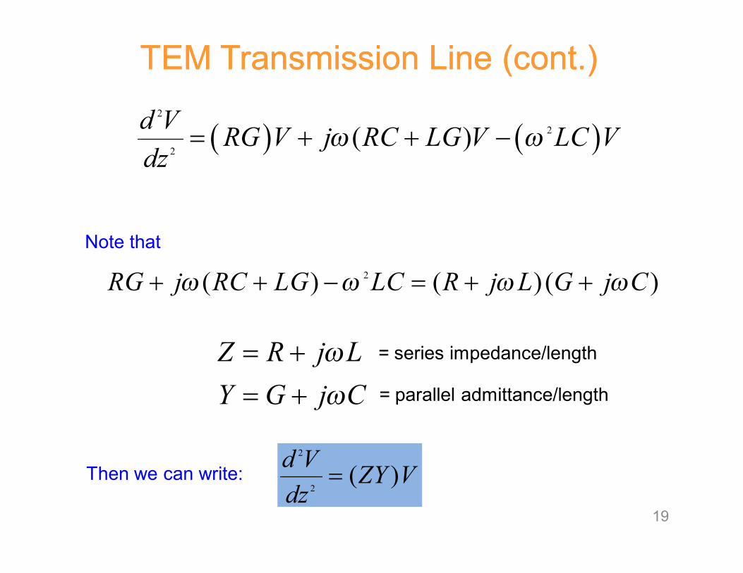
Note that

= series impedance/length

( ) ( )2

2

2( )d V RG V j RC LG V LC V

dzω ω= + + −

2( ) ( ) ( )RG j RC LG LC R j L G j Cω ω ω ω+ + − = + +

Z R j LY G j C

ωω

= += + = parallel admittance/length

Then we can write:2

2( )d V ZY V

dz=


19

Let

Convention:

Solution:

2γ = ZY

( ) z zV z Ae Beγ γ− += +

[ ]1/ 2( )( )R j L G j Cγ ω ω= + +

= principal square root

2

2

2( )d V V

dzγ=Then


γ is called the "propagation constant."

/2jz z e θ=

π θ π− < <

jγ α β= +

0, 0α β≥ ≥

αβ

==

attenuationcontant

phaseconstant

20


0 0( ) z z j zV z V e V e eγ α β+ + − + − −= =

Forward travelling wave (a wave traveling in the positive z direction):

( ) ( )

( )

0

0

0

( , ) Re

Re

cos

z j z j t

j z j z j t

z

v z t V e e e

V e e e e

V e t z

α β ω

φ α β ω

α ω β φ

+ + − −

+ − −

+ −

=

=

= − +

gλ0t =

z0

zV e α+ −

2

g

πβλ

=

2g

βλ π=

The wave “repeats” when:

Hence:

21

Phase VelocityPhase VelocityTrack the velocity of a fixed point on the wave (a point of constant phase), e.g., the crest.

0( , ) cos( )zv z t V e t zα ω β φ+ + −= − +

z

vp (phase velocity)

22

Phase Velocity (cont.)Phase Velocity (cont.)

0

constantω β

ω β

ωβ

− =

− =

=

t zdzdtdzdt

Set

Hence pv ω

β=

[ ] 1/2Im ( )( )pv

R j L G j Cω

ω ω=

+ +

In expanded form:

23

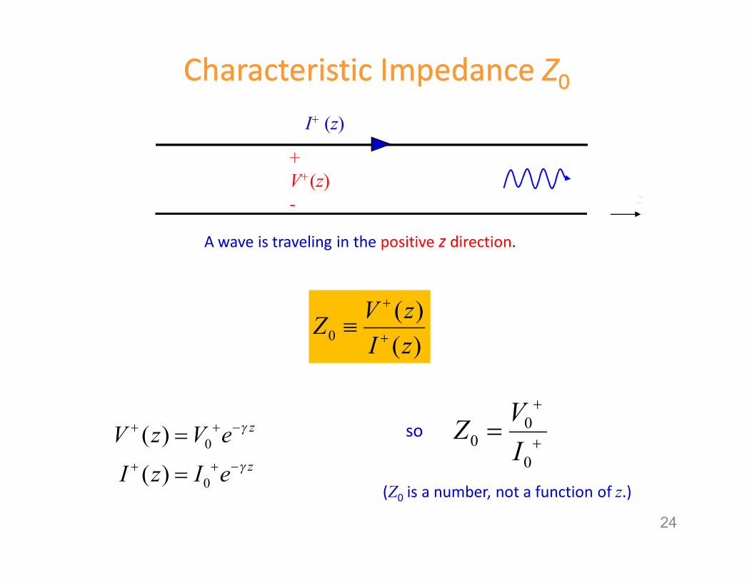
Characteristic Impedance Characteristic Impedance ZZ00

0( )( )

V zZI z

+

+≡

0

0

( )

( )

z

z

V z V eI z I e

γ

γ

+ + −

+ + −

=

=

so 00

0

VZI

+

+=

+ V+(z)-

I+ (z)

z

A wave is traveling in the positive z direction.

(Z0 is a number, not a function of z.)

24

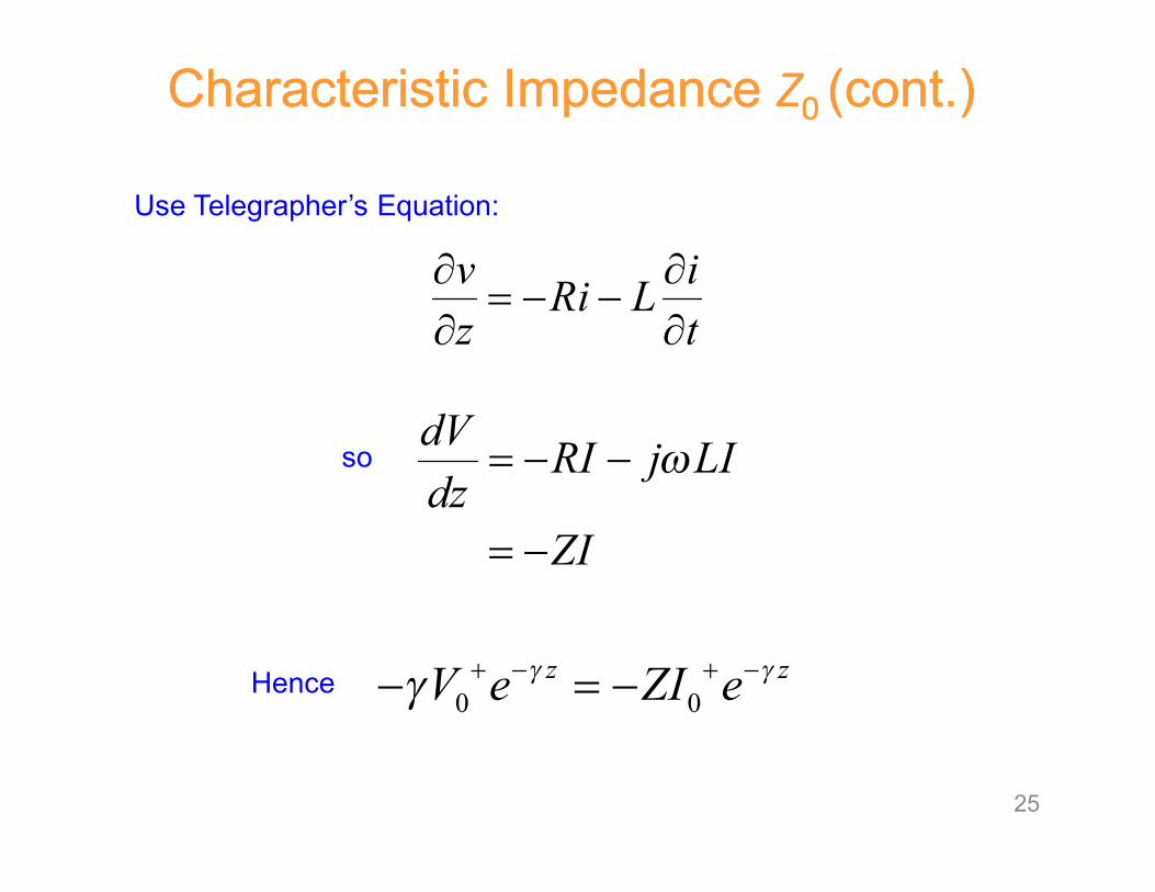
Use Telegrapher’s Equation:

v iRi Lz t

∂ ∂= − −

∂ ∂

sodV RI j LIdz

ZI

ω= − −

= −

Hence0 0

z zV e ZI eγ γγ + − + −− = −

Characteristic Impedance Characteristic Impedance ZZ0 0 (cont.) (cont.)

25

From this we have:

Using

We have

1/20

00

V Z ZZI Yγ

+

+ = = =

Y G j Cω= +

1/2

0R j LZG j C

ωω

+= +

Characteristic Impedance Characteristic Impedance ZZ0 0 (cont.) (cont.)

Z R j Lω= +

Note: The principal branch of the square root is chosen, so that Re (Z0) > 0. 26

( )

00

0 0

j z j j z

z z

z j zV e e

V z V e V

V e e e

e

eφ α

γ γ

ββ φ α−+

+ + −

−+ + − +

+

+

= +

= +

( ) ( ) ( )

( )0

0 cos

c

, R

os

e j t

z

z

V e t

v z t V z

z

V z

e

e t

ω

α

α

ω β

ω β φ

φ− +

+ +

−

−

+

=

+

+

+

−=

Note:wave in +zdirection wave in -z

direction

General Case General Case (Waves in Both Directions)(Waves in Both Directions)

27

BackwardBackward--Traveling WaveTraveling Wave

0( )( )

V z ZI z

−

− =− 0

( )( )

V z ZI z

−

− = −so

+ V -(z)-

I - (z)

z

A wave is traveling in the negative z direction.

Note: The reference directions for voltage and current are the same as for the forward wave.

28

General CaseGeneral Case

0 0

0 00

( )1( )

z z

z z

V z V e V e

I z V e V eZ

γ γ

γ γ

+ − − +

+ − − +

= +

= −

A general superposition of forward and backward traveling waves:

Most general case:

Note: The reference directions for voltage and current are the same for forward and backward waves.

29

+ V (z)-

I (z)

z

( )

( )

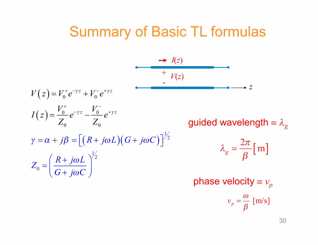
( )( )1

2

12

0

0 0

0 0

0 0

z z

z z

V z V e V e

V VI z e eZ

j R j L G j C

R j LZG j

Z

C

γ γ

γ γ

γ α β ω ω

ωω

+ − − +

+ −− +

=

= +

+ = + +

+=

=

−

+

[ ]2 mgπ

λβ

=

[m/s]pv ωβ

=

guided wavelength ≡ λg

phase velocity ≡ vp

Summary of Basic TL formulasSummary of Basic TL formulas

30

Lossless CaseLossless Case0, 0R G= =

[ ]1/ 2( )( )j R j L G j C

j LC

γ α β ω ω

ω

= + = + +

=

so 0

LC

α

β ω

=

=

1/2

0R j LZG j C

ωω

+= +

0LZC

=1

pvLC

=

pv ωβ

=

(indep. of freq.)(real and indep. of freq.)31

Lossless Case (cont.)Lossless Case (cont.)1

pvLC

=

In the medium between the two conductors is homogeneous (uniform) and is characterized by (ε, µ), then we have that

LC µε=

The speed of light in a dielectric medium is1

dcµε

=

Hence, we have that p dv c=

The phase velocity does not depend on the frequency, and it is always the speed of light (in the material).

(proof given later)

32

( ) 0 0z zV z V e V eγ γ+ − − += +

Where do we assign z = 0?

The usual choice is at the load.

l

Terminating impedance (load)

Ampl. of voltage wave propagating in negative zdirection at z = 0.

Ampl. of voltage wave propagating in positive zdirection at z = 0.

Terminated Transmission LineTerminated Transmission Line

Note: The length l measures distance from the load: z= −l33

What if we know

@V V z+ − = −land

( ) ( )0 0V V V e γ+ + + −= = − ll

( ) ( ) ( ) ( ) ( )z zV z V e V eγ γ− + ++ −= − + −l ll l

( ) ( )0V V e γ− − −− = ll

( ) ( )0 0V V V eγ− − −⇒ = = − ll

Terminated Transmission Line (cont.)Terminated Transmission Line (cont.)

( ) 0 0z zV z V e V eγ γ+ − − += +

Hence

Can we use z = - l as a reference plane?

l


34

( ) ( ) ( ) ( ) ( )( ) ( )z zV z V e V eγ γ− − − − −+ −= − + −l ll l


( ) ( ) ( )0 0z zV z V e V eγ γ+ − − += +

Compare:

Note: This is simply a change of reference plane, from z = 0 to z = -l.

l


35

( ) 0 0z zV z V e V eγ γ+ − − += +

What is V(-l )?

( ) 0 0V V e V eγ γ+ − −− = +l ll

( ) 0 0

0 0

V VI e eZ Z

γ γ+ −

−− = −l ll

propagating forwards

propagating backwards


l ≡ distance away from load

The current at z = - l is then

l


36

( ) ( )20

0

1 LVI e eZ

γ γ+

−− = − Γl ll

( ) 200

00 0 1 VV eV V e ee

VV γ γγ γ

−+− −+ −

+− =

= +

+ l ll ll

Total volt. at distance lfrom the load

Ampl. of volt. wave prop. towards load, at the load position (z = 0).

Similarly,

Ampl. of volt. wave prop. away from load, at the load position (z = 0).

( )021 LV e eγ γ+ −= + Γl l

ΓL ≡ Load reflection coefficient


0 ,Z γ

Γl ≡ Reflection coefficient at z = - l

37

( ) ( )

( ) ( )

( ) ( )( )

20

2

2

0

0

2

0

11

1

1

L

L

L

L

V V e e

VI e eZ

V eZ ZI e

γ γ

γ γ

γ

γ

+ −

+

−

−

−

− = + Γ

− + Γ− = = − −

− = −Γ

Γ

l l

l

l

l

l

ll

l

l

l

Input impedance seen “looking” towards load at z = -l .


0 ,Z γ

( )Z −l

38

At the load (l = 0):

( ) 0101

LL

L

Z Z Z + Γ

= − Γ≡

Thus,

( )

20

00

20

0

1

1

L

L

L

L

Z Z eZ Z

Z ZZ Z eZ Z

γ

γ

−

−

−+ + − = −− +

l

l

l


0

0

LL

L

Z ZZ Z

−⇒ Γ =

+

( )2

0 2

11

L

L

eZ Ze

γ

γ

−

−

+ Γ− = −Γ

l

llRecall

39

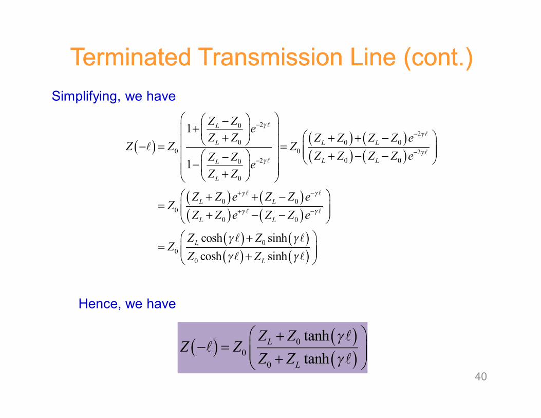
Simplifying, we have

( ) ( )( )

00

0

tanhtanh

L

L

Z ZZ Z

Z Zγγ

+− = +

ll

l


( ) ( ) ( )( ) ( )

( ) ( )( ) ( )

( ) ( )( ) ( )

202

0 0 00 0 2

2 0 00

0

0 00

0 0

00

0

1

1

cosh sinhcosh sinh

L

L L L

L LL

L

L L

L L

L

L

Z Z eZ Z Z Z Z Z e

Z Z ZZ Z Z Z eZ Z e

Z Z

Z Z e Z Z eZ

Z Z e Z Z e

Z ZZ

Z Z

γγ

γγ

γ γ

γ γ

γ γγ γ

−−

−−

+ −

+ −

−+ + + + − − = = + − − − − +

+ + −= + − −

+= +

l

l

ll

l l

l l

l

l l

l l

Hence, we have

40

( ) ( )

( ) ( )

( )

20

20

0

2

0 2

1

1

11

j jL

j jL

jL

jL

V V e e

VI e eZ

eZ Ze

β β

β β

β

β

+ −

+−

−

−

− = + Γ

− = − Γ

+ Γ− = −Γ

l l

l l

l

l

l

l

l

Impedance is periodic with period λg/2

2

/ 2g

g

β ππ

πλ

λ

=

=

⇒ =

l

l

l

Terminated Lossless Transmission LineTerminated Lossless Transmission Line

j jγ α β β= + =

Note: ( ) ( ) ( )tanh tanh tanj jγ β β= =l l l

tan repeats when

( ) ( )( )

00

0

tantan

L

L

Z jZZ Z

Z jZββ

+− = +

ll

l

41

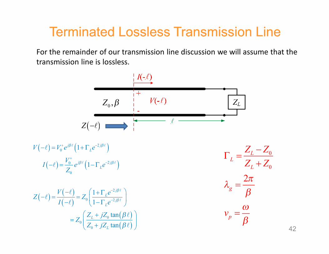
For the remainder of our transmission line discussion we will assume that the transmission line is lossless.

( ) ( )

( ) ( )

( ) ( )( )

( )( )

20

20

0

2

0 2

00

0

1

1

11

tantan

j jL

j jL

jL

jL

L

L

V V e e

VI e eZ

V eZ ZI e

Z jZZ

Z jZ

β β

β β

β

β

ββ

+ −

+−

−

−

− = + Γ

− = − Γ

− + Γ− = = − − Γ

+= +

l l

l l

l

l

l

l

ll

l

l

l

0

0

2

LL

L

g

p

Z ZZ Z

v

πλ

βωβ

−Γ =

+

=

=

Terminated Lossless Transmission LineTerminated Lossless Transmission Line

0 ,Z β

( )Z −l

42

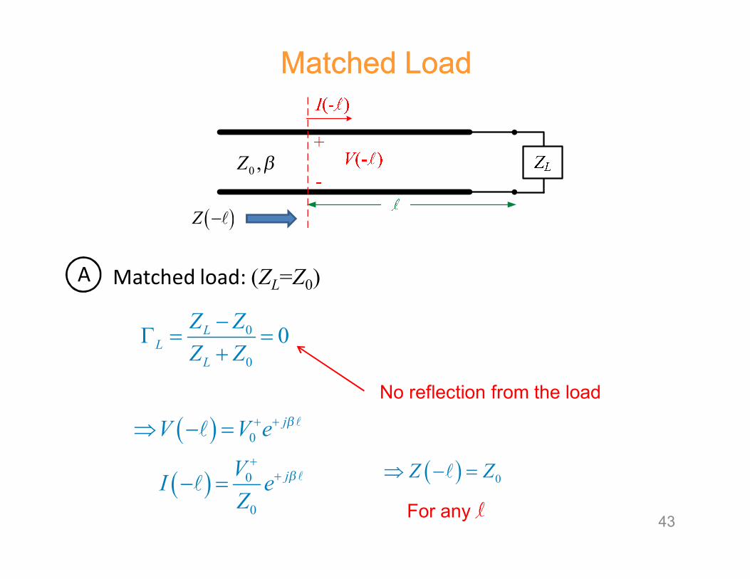
Matched load: (ZL=Z0)

0

0

0LL

L

Z ZZ Z

−Γ = =

+

For any l

No reflection from the load

A

Matched LoadMatched Load

0 ,Z β

( )Z −l

( ) 0Z Z⇒ − =l

( )

( )

0

0

0

j

j

V V e

VI eZ

β

β

+ +

++

⇒ − =

− =

l

l

l

l

43

Short circuit load: (ZL = 0)

( ) ( )

0

0

0

0 10

tan

LZZ

Z jZ β

−Γ = = −

+

⇒ − =l l

Always imaginary!Note:

B

2g

β πλ

=ll

( ) scZ jX⇒ − =l

S.C. can become an O.C. with a λg/4 trans. line

g/ λl

ShortShort--Circuit LoadCircuit Load

0 ,Z β

( )0 tanscX Z β= l

44

Using Transmission Lines to Synthesize LoadsUsing Transmission Lines to Synthesize Loads

A microwave filter constructed from microstrip.

This is very useful is microwave engineering.

45

( ) ( )( )

00

0

tantan

Lin

L

Z jZ dZ Z d Z

Z jZ dββ

+= − = +

( ) inTH

in TH

ZV d VZ Z

⇒ − = +

0Z β=

ExampleExample

Find the voltage at any point on the line.

46

Note: ( ) ( )021 j

LjV V e eβ β+ −+ Γ=− l ll

0

0

LL

L

Z ZZ Z

−Γ =

+

( ) ( )20 1j d j d in

THin TH

LV d ZZ

e VZ

V e β β+ −− = + Γ

= +

( ) ( )2

2

11

jj din L

TH j dm TH L

Z eV V eZ Z e

ββ

β

−− −

−

+ Γ− = + + Γ

lll

At l = d :

Hence

Example (cont.) Example (cont.)

0 2

11

j dinTH j d

in TH L

ZV V eZ Z e

ββ

+ −−

⇒ = + + Γ

47

Some algebra: ( )2

0 2

11

j dL

in j dL

eZ Z d Ze

β

β

−

−

+ Γ= − = − Γ

( )( ) ( )

( )( ) ( )

( )

2

20 20

2 220

0 2

20

20 0

20

20 0

0

111

1 111

1

1

1

j dL

j dj dLL

j d j dj dL TH LL

THj dL

j dL

j dTH L TH

j dL

j dTH THL

TH

in

in TH

eZ Z eeZ e Z eeZ Z

e

Z eZ Z e Z Z

eZZ

ZZ Z

Z Z ZeZ Z

Z

β

ββ

β ββ

β

β

β

β

β

−

−−

− −−

−

−

−

−

−

+ Γ + Γ− Γ ⇒ = =

+ Γ + − Γ+ Γ + − Γ

+ Γ=

+ + Γ

+

−

+ Γ = + − + Γ +

=( )2

0

20 0

0

1

1

j dL

j dTH THL

TH

eZ Z Z Ze

Z Z

β

β

−

−

+ Γ + − − Γ +


48

( ) ( )2

02

0

11

jj d L

TH j dTH S L

Z eV V eZ Z e

ββ

β

−− −

−

+ Γ− = + − Γ Γ

lll

20

20

11

j din L

j din TH TH S L

Z Z eZ Z Z Z e

β

β

−

−

+ Γ= + + − Γ Γ

where 0

0

THS

TH

Z ZZ Z

−Γ =

+


Therefore, we have the following alternative form for the result:

Hence, we have

49

( ) ( )2

02

0

11

jj d L

TH j dTH S L

Z eV V eZ Z e

ββ

β

−− −

−

+ Γ− = + − Γ Γ

ll

l


0Z β=

Voltage wave that would exist if there were no reflections from the load (a semi-infinite transmission line or a matched load).

50

( )( )

( ) ( ) ( ) ( )

2 2

2 2 2 20

0

1 j d j dL L S

j d j d j d j dTH L S L L S L S

TH

e eZV d V e e e e

Z Z

β β

β β β β

− −

− − − −

+ Γ + Γ Γ − = + Γ Γ Γ + Γ Γ Γ Γ + +

K


0Z β=

Wave-bounce method (illustrated for l = d):

51


( )

( ) ( )( ) ( )

22 2

22 2 20

0

1

1

j d j dL S L S

j d j d j dTH L L S L S

TH

e eZV d V e e e

Z Z

β β

β β β

− −

− − −

+ Γ Γ + Γ Γ +

− = + Γ + Γ Γ + Γ Γ + + +

K

K

K

Geometric series:

2

0

11 , 11

n

nz z z z

z

∞

=

= + + + = <−∑ K

( )( )

( ) ( ) ( ) ( )

2 2

2 2 2 20

0

1 j d j dL L S

j d j d j d j dTH L S L L S L S

TH

e eZV d V e e e e

Z Z

β β

β β β β

− −

− − − −

+ Γ + Γ Γ − = + Γ Γ Γ + Γ Γ Γ Γ + +

K

2j dL Sz e β−= Γ Γ

52


or

( )2

0

202

11

11

j dL s

THj dTH

L j dL s

eZV d VZ Z

ee

β

ββ

−

−−

− Γ Γ − = + + Γ − Γ Γ

( )2

02

0

11

j dL

TH j dTH L s

Z eV d VZ Z e

β

β

−

−

+ Γ− = + − Γ Γ

This agrees with the previous result (setting l = d).

Note: This is a very tedious method – not recommended.

Hence

53

I(- )

V(- )+

ZL-

0 ,Z γ

At a distance l from the load:

( ) ( ) ( )

( )( )*

*

2

0 2 2 * 2*0

1 Re 1 1

1 R

2

e2

L L

Ve e

Z

V I

e

P

α γ γ+

− −

− =

= + Γ −Γ

− −

l l l

l l l

( ) ( )2

20 2 4

0

1 12 L

VP e e

Zα α

+−− ≈ − Γl ll

If Z0 ≈ real (low-loss transmission line)

TimeTime-- Average Power FlowAverage Power Flow

( ) ( )

( ) ( )

20

20

0

1

1

L

L

V V e e

VI e eZj

γ γ

γ γ

γ α β

+ −

+−

− = + Γ

− = −Γ

= +

l l

l l

l

l

( )

*2 * 2

*2 2

L L

L L

e e

e e

γ γ

γ γ

− −

− −

Γ − Γ

= Γ − Γ

=

l l

l l

pure imaginary

Note:

54

Low-loss line

( ) ( )2

20 2 4

0

2 2

20 02 2* *0 0

1 12

1 12 2

L

L

VP d e e

Z

V Ve e

Z Z

α α

α α

+−

+ +−

− ≈ − Γ

= − Γ

l l

l l

14243 1442443power in forward wave power in backward wave

( ) ( )2

20

0

1 12 L

VP d

Z

+

− = − Γ

Lossless line (α = 0)

TimeTime-- Average Power FlowAverage Power FlowI(- )

V(- )+

ZL-

0 ,Z γ

55

00

0

tantan

L Tin T

T L

Z jZZ ZZ jZ

ββ

+= +

l

l

24 4 2

g g

g

λ λπ πβ β

λ= = =l

00

Tin T

L

jZZ ZjZ

⇒ =

0

20

0

0in in

T

L

Z Z

ZZZ

Γ = ⇒ =

⇒ =

QuarterQuarter--Wave TransformerWave Transformer

20T

inL

ZZZ

=so

[ ]1/20 0T LZ Z Z=

Hence

This requires ZL to be real.

ZLZ0 Z0T

Zin

56

( ) 20 1 Lj j

LV V e eφ β+ −− = + Γ ll

( ) ( )( )

20

20

1

1 L

j jL

jj jL

V V e e

V e e e

β β

φβ β

+ −

+ −

− = + Γ

= + Γ

l l

l l

l

( )( )

max 0

min 0

1

1

L

L

V V

V V

+

+

= + Γ

= − Γ

( ) max

min

VV

=Voltage Standing Wave Ratio VSWR

Voltage Standing Wave RatioVoltage Standing Wave RatioI(- )

V(- )+

ZL-

0 ,Z γ

11

L

L

+ Γ=

− ΓVSWR

z

1+ LΓ

1

1- LΓ

0

( )V zV +

/ 2z λ∆ =0z =

57

Coaxial CableCoaxial CableHere we present a “case study” of one particular transmission line, the coaxial cable.

a

b ,rε σ

Find C, L, G, R

We will assume no variation in the z direction, and take a length of one meter in the zdirection in order top calculate the per-unit-length parameters.

58

For a TEMz mode, the shape of the fields is independent of frequency, and hence we can perform the calculation using electrostatics and magnetostatics.

Coaxial Cable (cont.)Coaxial Cable (cont.)

-ρl0

ρl0

a

b

rε0 0

0

ˆ ˆ2 2 r

E ρ ρρ ρ

π ε ρ π ε ε ρ

= =

l l

Find C (capacitance / length)

Coaxial cable

h = 1 [m]

rε

From Gauss’s law:

0

0

ln2

B

ABA

b

ra

V V E dr

bE daρ

ρρ

π ε ε

= = ⋅

= =

∫

∫ l

59

-ρl0

ρl0

a

b

rε

Coaxial cable

h = 1 [m]

rε

( )0

0

0

1

ln2 r

QCV b

a

ρ

ρπ ε ε

= =

l

l

Hence

We then have

0 F/m2 [ ]ln

rCba

π ε ε=


60

ˆ2

IH φπ ρ

=

Find L (inductance / length)

From Ampere’s law:

Coaxial cable

h = 1 [m]

rµ

I

0ˆ

2 rIB φ µ µ

π ρ

=

(1)b

a

B dφψ ρ= ∫S

h

I

Iz

center conductorMagnetic flux:


61

Note: We ignore “internal inductance” here, and only look at the magnetic field between the two conductors (accurate for high frequency.

Coaxial cable

h = 1 [m]

rµ

I

( ) 0

0

0

1

2

ln2

b

ra

b

ra

r

H d

I d

I ba

φψ µ µ ρ

µ µ ρπρ

µ µπ

=

=

=

∫

∫

01 ln

2rbL

I aψ µ µ

π = =

0 H/mln [ ]2

r bLa

µ µπ

=

Hence


62

0 H/mln [ ]2

r bLa

µ µπ

=

Observation:

0 F/m2 [ ]ln

rCba

π ε ε=

( )0 0 r rLC µε µ ε µ ε= =

This result actually holds for any transmission line.


63

0 H/mln [ ]2

r bLa

µ µπ

=

For a lossless cable:

0 F/m2 [ ]ln

rCba

πε ε=

0LZC

=

0 01 ln [ ]

2r

r

bZa

µη

ε π = Ω

00

0

376.7303 [ ]µη

ε= = Ω


64

-ρl0

ρl0

a

b

σ0 0

0

ˆ ˆ2 2 r

E ρ ρρ ρ

π ε ρ π ε ε ρ

= =

l l

Find G (conductance / length)

Coaxial cable

h = 1 [m]

σ

From Gauss’s law:

0

0

ln2

B

ABA

b

ra

V V E dr

bE daρ

ρρ

π ε ε

= = ⋅

= =

∫

∫ l


65

-ρl0

ρl0

a

b

σ J Eσ=

We then have leakIGV

=

[ ]

0

0

(1) 2

2

22

leak a

a

r

I J a

a E

aa

ρ ρ

ρ ρ

π

π σ

ρπ σ

π ε ε

=

=

=

=

=

l

0

0

0

0

22

ln2

r

r

aa

Gba

ρπ σ

π ε ερ

π ε ε

=

l

l

2 [S/m]ln

Gba

πσ=

or


66

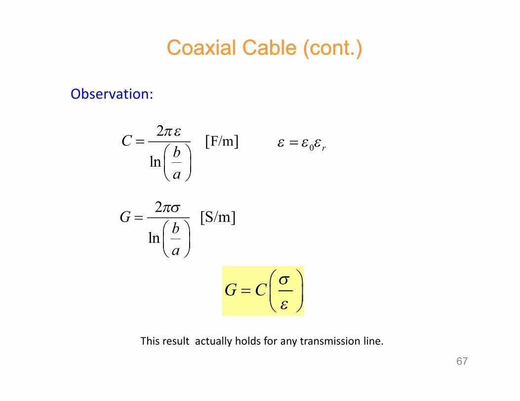
Observation:

F/m2 [ ]

lnC

ba

πε=

G C σε

=

This result actually holds for any transmission line.

2 [S/m]ln

Gba

πσ=

0 rε ε ε=


67

G C σε

=

To be more general:

tanGC

σδ

ω ωε = =

tanGC

δω

=

Note: It is the loss tangent that is usually (approximately) constant for a material, over a wide range of frequencies.


As just derived,

The loss tangent actually arises from both conductivity loss and polarization loss (molecular friction loss), ingeneral.

68

This is the loss tangent that would arise from conductivity effects.

General expression for loss tangent:

( )

c

c c

j

j j

j

σε ε

ωσ

ε εω

ε ε

= −

′ ′′= − −

′ ′′= −

tan c

c

σεε ωδ

εε

′′ + ′′ ≡ =′′

Effective permittivity that accounts for conductivity

Loss due to molecular friction Loss due to conductivity


69

Find R (resistance / length)

Coaxial cable

h = 1 [m]


,b rbσ µ

a

b

σ,a raσ µ

a bR R R= +

12a saR R

aπ =

12b sbR R

bπ =

1sa

a a

Rσ δ

=1

sbb b

Rσ δ

=

0

2a

ra a

δωµ µ σ

=0

2b

rb b

δωµ µ σ

=

Rs = surface resistance of metal

70

General Transmission Line FormulasGeneral Transmission Line Formulas

tanGC

δω

=

( )0 0 r rLC µε µ ε µ ε′ ′= =

0losslessL Z

C= = characteristic impedance of line (neglecting loss)(1)

(2)

(3)

Equations (1) and (2) can be used to find L and C if we know the material properties and the characteristic impedance of the lossless line.

Equation (3) can be used to find G if we know the material loss tangent.

a bR R R= +

tanGC

δω

=(4)

Equation (4) can be used to find R (discussed later).

,iC i a b= =contour of conductor,

22

1 ( )i

i s szC

R R J l dlI

=

∫

71

General Transmission Line Formulas (cont.)General Transmission Line Formulas (cont.)

( ) tanG Cω δ=

0losslessL Z µε ′=

0/ losslessC Zµε ′=

R R=

Al four per-unit-length parameters can be found from 0 ,losslessZ R

72

Common Transmission LinesCommon Transmission Lines

0 01 ln [ ]

2lossless r

r

bZa

µη

ε π = Ω

Coax

Twin-lead

100 cosh [ ]

2lossless r

r

hZa

η µπ ε

− = Ω

2

1 2

12

s

haR R

a ha

π

= −

1 12 2sa sbR R R

a bπ π = +

a

b

,r rε µ

h

,r rε µ

a a

73

Common Transmission Lines (cont.) Common Transmission Lines (cont.)

Microstrip

( ) ( ) ( )( )

( )( )0 0

1 00

0 1

eff effr reff effr r

fZ f Z

fε εε ε

−= −

( )( ) ( ) ( )( )0

12000 / 1.393 0.667 ln / 1.444eff

r

Zw h w h

π

ε=

′ ′+ + +

( / 1)w h ≥

21 lnt hw wtπ

′ = + +

h

w

εr

t

74

Common Transmission Lines (cont.) Common Transmission Lines (cont.)

Microstrip ( / 1)w h ≥

h

w

εr

t

( )2

1.5

(0)(0)

1 4

effr reff eff

r rfF

ε εε ε −

− = + +

( )( )

1 1 11 /02 2 4.6 /1 12 /

eff r r rr

t hw hh w

ε ε εε

+ − − = + − +

2

0

4 1 0.5 1 0.868ln 1rh wF

hε

λ

= − + + +

75

At high frequency, discontinuity effects can become important.

Limitations of TransmissionLimitations of Transmission--Line TheoryLine Theory

Bend

incident

reflected

transmitted

The simple TL model does not account for the bend.

ZTH

ZLZ0+-

76

At high frequency, radiation effects can become important.

When will radiation occur?

We want energy to travel from the generator to the load, without radiating.

Limitations of TransmissionLimitations of Transmission--Line Theory (cont.)Line Theory (cont.)

ZTH

ZLZ0+-

77

rε a

bz

The coaxial cable is a perfectly shielded system – there is never any radiation at any frequency, or under any circumstances.

The fields are confined to the region between the two conductors.


78

The twin lead is an open type of transmission line – the fields extend out to infinity.

The extended fields may cause interference with nearby objects. (This may be improved by using “twisted pair.”)

+ -


Having fields that extend to infinity is not the same thing as having radiation, however.

79

The infinite twin lead will not radiate by itself, regardless of how far apart the lines are.

h

incident

reflected

The incident and reflected waves represent an exact solution to Maxwell’s equations on the infinite line, at any frequency.

( )*1 ˆRe E H 02t

S

P dSρ = × ⋅ = ∫

S

+ -


No attenuation on an infinite lossless line

80

A discontinuity on the twin lead will cause radiation to occur.

Note: Radiation effects increase as the frequency increases.


h

Incident wavepipe

obstacle

Reflected wave

bend h

Incident wave

bend

Reflected wave 81

To reduce radiation effects of the twin lead at discontinuities:

h

1) Reduce the separation distance h (keep h << λ).2) Twist the lines (twisted pair).


CAT 5 cable(twisted pair)

82

Documents

RF Communication Circuits - Sharif University of Technologyee.sharif.edu/~comm_cir-AliF/Note2.pdf · RF Communication Circuits Lecture 2: ... A microwave integrated circuit ... We