RFI: Sources,

Identification, Mitigation (part 1)

Brian Corey

2

Effects of RFI on VLBI

RFI increases system temperature. Depending on strength of RFI , it may affect only those frequency channels where RFI is present, or all frequency channels if RFI is strong enough to overload electronics.

Effects of increased Tsys include: Reduction in SNR and hence in geodetic/astrometric precision and

astronomical source mapping quality Systematic shifts in estimated group delay (see next slide) Failure of geodetic bandwidth synthesis if too many frequency channels are

severely affected by RFI E.g., in T2075 RFI caused loss of channels S1 and S5 at station A and

S2 and S3 in station B, leaving only two usable channels on baseline AB. SNR is inversely proportional to

sqrt[ 1 + (RFI power integrated over channel BW) / ( non-RFI power) ]. E.g., if RFI power = 50% of non-RFI, SNR drops by 18%. In continuum VLBI, don’t worry about every little narrowband RFI spike, as

its total power may be insignificant. In spectral-line VLBI, do worry if spike falls on top of your spectral line!

3

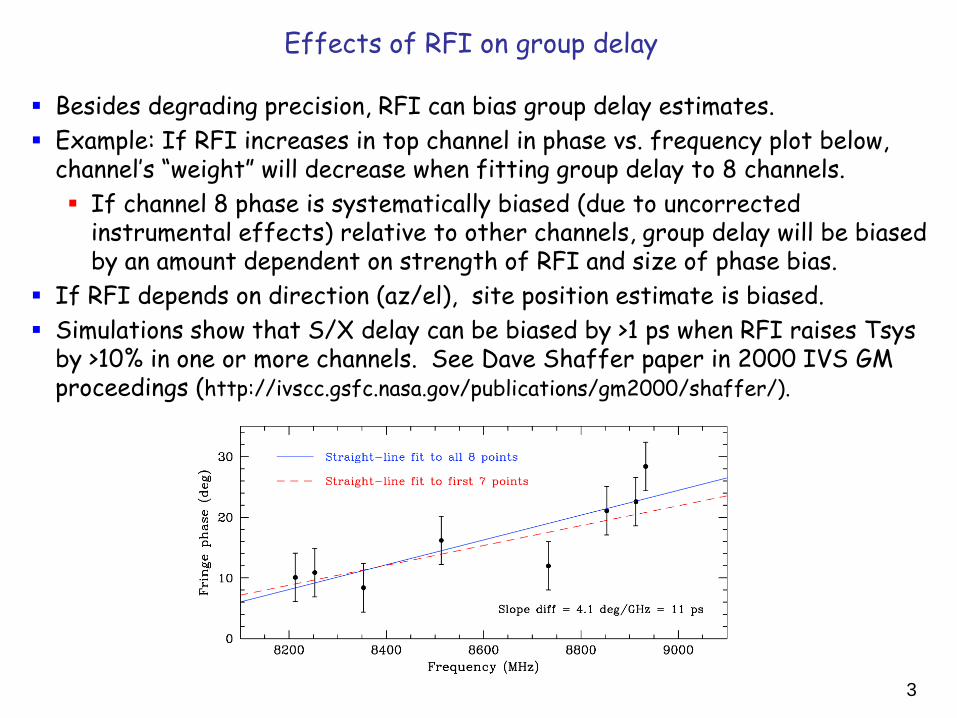
Effects of RFI on group delay

Besides degrading precision, RFI can bias group delay estimates. Example: If RFI increases in top channel in phase vs. frequency plot below,

channel’s “weight” will decrease when fitting group delay to 8 channels. If channel 8 phase is systematically biased (due to uncorrected

instrumental effects) relative to other channels, group delay will be biased by an amount dependent on strength of RFI and size of phase bias.

If RFI depends on direction (az/el), site position estimate is biased. Simulations show that S/X delay can be biased by >1 ps when RFI raises Tsys

by >10% in one or more channels. See Dave Shaffer paper in 2000 IVS GM proceedings (http://ivscc.gsfc.nasa.gov/publications/gm2000/shaffer/).

4

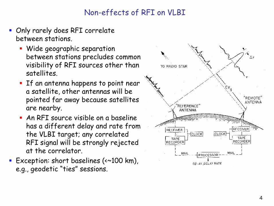
Non-effects of RFI on VLBI

Only rarely does RFI correlate between stations. Wide geographic separation

between stations precludes common visibility of RFI sources other than satellites.

If an antenna happens to point near a satellite, other antennas will be pointed far away because satellites are nearby.

An RFI source visible on a baseline has a different delay and rate from the VLBI target; any correlated RFI signal will be strongly rejected at the correlator.

Exception: short baselines (<~100 km), e.g., geodetic “ties” sessions.

5

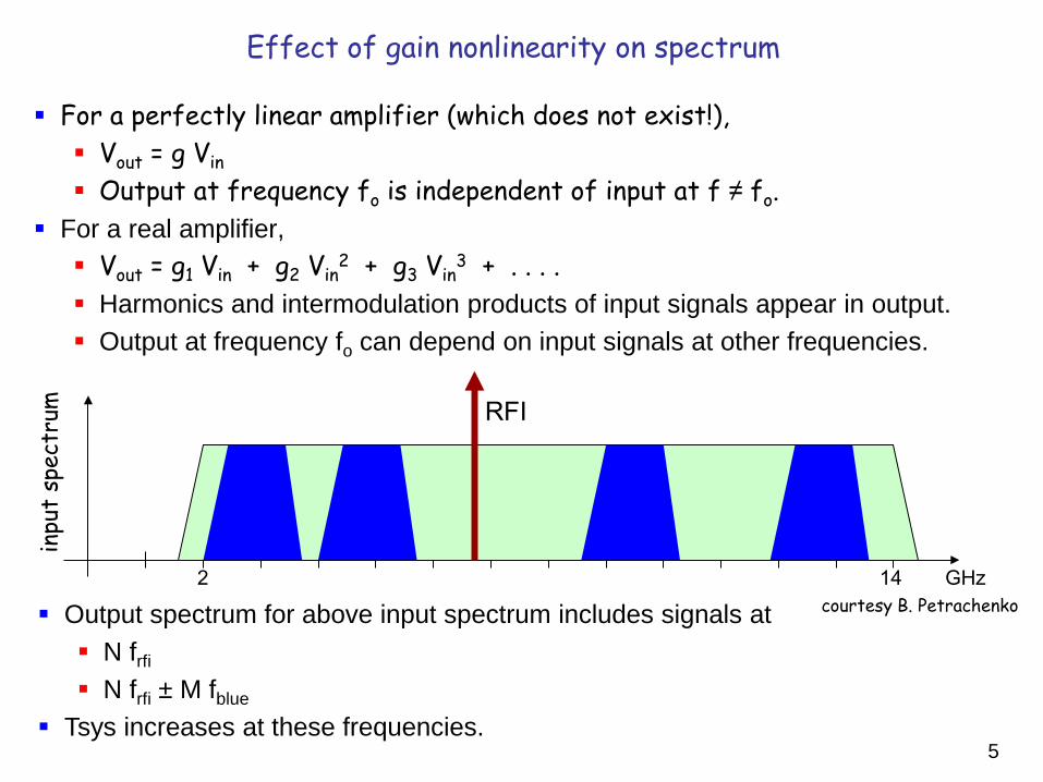
Effect of gain nonlinearity on spectrum

For a perfectly linear amplifier (which does not exist!), Vout = g Vin

Output at frequency fo is independent of input at f ≠ fo. For a real amplifier, Vout = g1 Vin + g2 Vin

2 + g3 Vin3 + . . . .

Harmonics and intermodulation products of input signals appear in output. Output at frequency fo can depend on input signals at other frequencies.

2 14 GHz

RFI

Output spectrum for above input spectrum includes signals at N frfi N frfi ± M fblue

Tsys increases at these frequencies.

inpu

t sp

ectr

um

courtesy B. Petrachenko

6

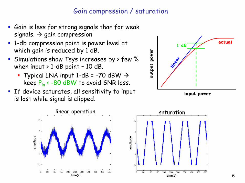
Gain compression / saturation

Gain is less for strong signals than for weak signals. gain compression

1-db compression point is power level at which gain is reduced by 1 dB.

Simulations show Tsys increases by > few % when input > 1-dB point – 10 dB. Typical LNA input 1-dB = -70 dBW

keep Pin < -80 dBW to avoid SNR loss. If device saturates, all sensitivity to input

is lost while signal is clipped. linear operation saturation

7

When should I worry that RFI is too strong?

You should worry when . . . RFI power raises system power in baseband frequency channel by >10%. Effects: SNR is reduced. Group delay may be biased significantly.

Frequency of RFI may lie outside frequency channel, but gain nonlinearity in VLBI system can “move” RFI into frequency channel.

RFI is at integer MHz, coherent with maser, and > -50 dB relative to phase cal signal. RFI = spurious phase cal signal, which degrades calibration.

RFI power > device survival limit Typical input limit for LNA is ~ -20 dBW.

Do not worry about every little blip on a spectrum analyzer! A signal 10 dB above the noise and 10 kHz wide adds only 1% to total

power of an 8-MHz-wide channel. not a problem for continuum VLBI

8

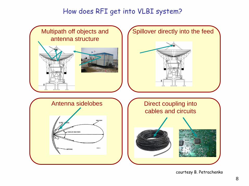
How does RFI get into VLBI system?

Multipath off objects and antenna structure

Spillover directly into the feed

Antenna sidelobes Direct coupling into cables and circuits

courtesy B. Petrachenko

9

Sources of RFI

RFI external to VLBI system Usually originates at RF frequencies and is picked up in feed. Can be at image frequency if RFI is strong enough to overcome image

rejection in receiver or backend. Can be picked up at IF frequencies if RFI is exceptionally strong,

especially if an IF cable has a broken shield or bad connector. Common RFI sources: Satellites Wireless/mobile/cell transmitters TV/radio broadcast and relay Radar

Internally generated RFI RF or IF amplifiers may oscillate. LNAs are especially prone to oscillation, which may occur at RF or IF

frequency. Backends (formatter) generate maser-coherent tones. Good practice: Set LOs of unused BBCs to frequencies outside observing

band.

10

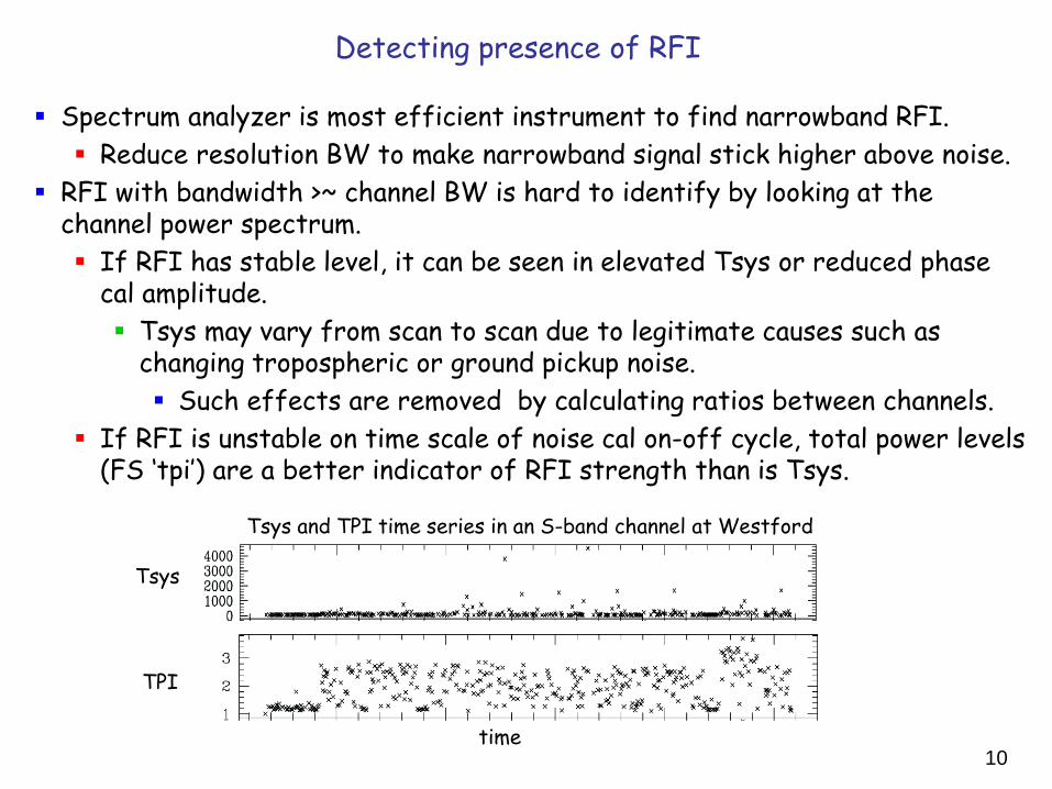
Detecting presence of RFI

Spectrum analyzer is most efficient instrument to find narrowband RFI. Reduce resolution BW to make narrowband signal stick higher above noise.

RFI with bandwidth >~ channel BW is hard to identify by looking at the channel power spectrum. If RFI has stable level, it can be seen in elevated Tsys or reduced phase

cal amplitude. Tsys may vary from scan to scan due to legitimate causes such as

changing tropospheric or ground pickup noise. Such effects are removed by calculating ratios between channels.

If RFI is unstable on time scale of noise cal on-off cycle, total power levels (FS ‘tpi’) are a better indicator of RFI strength than is Tsys.

Tsys

TPI

time

Tsys and TPI time series in an S-band channel at Westford

11

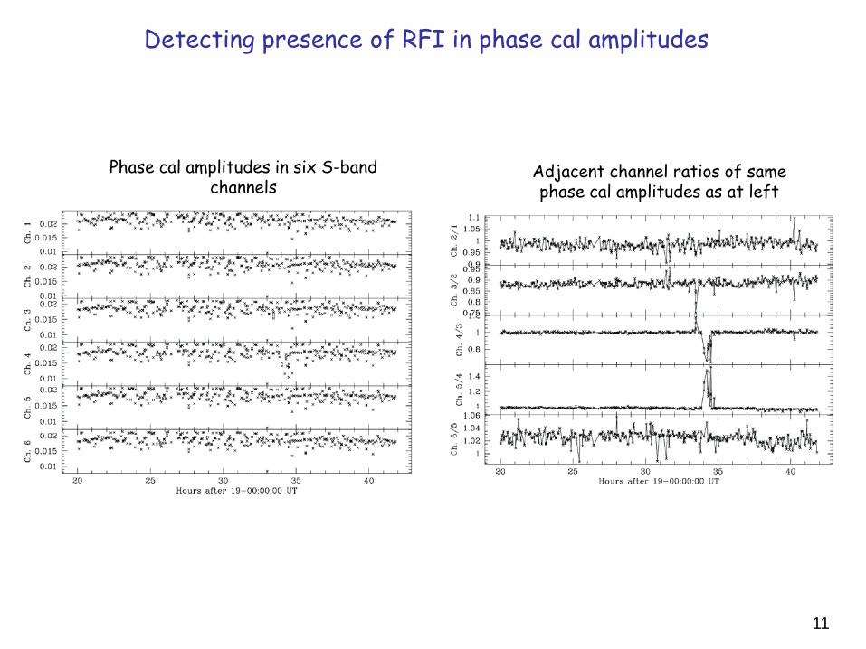
Detecting presence of RFI in phase cal amplitudes

Phase cal amplitudes in six S-band channels

Adjacent channel ratios of same phase cal amplitudes as at left

12

What can be done about RFI?

To reduce out-of-band RFI, install filters with sharp cutoffs. Options are limited if RFI drives LNA close to saturation.

Operate analog electronics and sampler at lowest level consistent with negligible impact on SNR, to maximize headroom and minimize potential for saturation.

Try to get cooperation of agency operating interferer, e.g. time multiplexing. Change observing frequencies to avoid persistent RFI. Has been done in geodesy to accommodate RFI at Matera, Medicina, and

Westford, among others. Avoid observing in direction toward interferer. Will have negative impact on geodetic results.

If RFI is internally generated . . . Fix the oscillating LNA. Fix the broken shield on the IF cable coming into the rack.

13

RFI and VGOS (VLBI2010)

VGOS frequency range of 2-14 GHz presents challenges from RFI. Mitigation strategies include: Use flexible tuning of updown converters to place radio-quiet observing

bands (500-1000 MHz wide) in between RFI-loud regions. Exclude RFI-loud regions within a band by recording selected narrow-BW

(e.g., 32 MHz) channels in each band. Use highly frequency selective techniques (e.g., high image rejection and

inter-channel isolation) in downconversion, Nyquist zone filtering and channel definition to keep RFI at one frequency from infecting another.

Use physical barriers to reduce interference from DORIS beacons and SLR aircraft surveillance radar at integrated geodetic sites.

Do not attempt to support observations below 2.2 GHz, where RFI is particularly strong; take advantage of highpass character of feed. GNSS observations may be precluded for main VGOS antenna; they

may be supported with a smaller reference antenna. But these strategies are useless if strong RFI in 2.2-14 GHz VGOS band

saturates LNA!

14

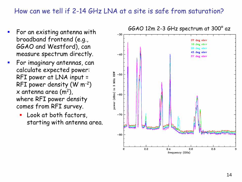
How can we tell if 2-14 GHz LNA at a site is safe from saturation?

For an existing antenna with broadband frontend (e.g., GGAO and Westford), can measure spectrum directly.

For imaginary antennas, can calculate expected power: RFI power at LNA input = RFI power density (W m-2) x antenna area (m2), where RFI power density comes from RFI survey. Look at both factors,

starting with antenna area.

GGAO 12m 2-3 GHz spectrum at 300° az

15

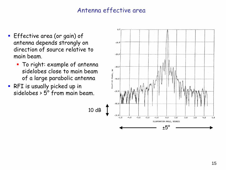
Antenna effective area

Effective area (or gain) of antenna depends strongly on direction of source relative to main beam. To right: example of antenna

sidelobes close to main beam of a large parabolic antenna

RFI is usually picked up in sidelobes > 5° from main beam.

10 dB

±5°

16

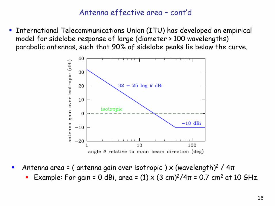
Antenna effective area – cont’d

International Telecommunications Union (ITU) has developed an empirical model for sidelobe response of large (diameter > 100 wavelengths) parabolic antennas, such that 90% of sidelobe peaks lie below the curve.

Antenna area = ( antenna gain over isotropic ) x (wavelength)2 / 4π Example: For gain = 0 dBi, area = (1) x (3 cm)2/4π = 0.7 cm2 at 10 GHz.

17

GGAO 12m antenna sidelobe pattern (dBi) at 9 GHz

18

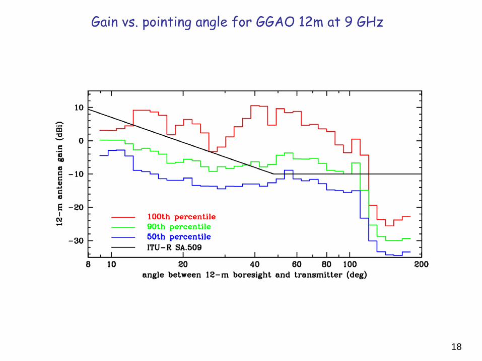
Gain vs. pointing angle for GGAO 12m at 9 GHz

19

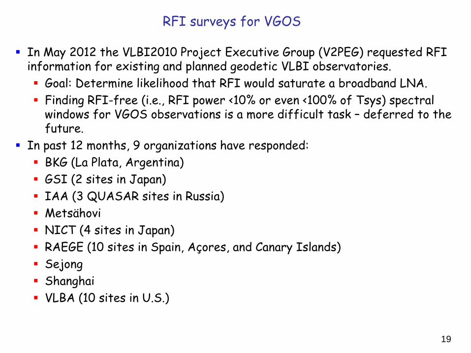
RFI surveys for VGOS

In May 2012 the VLBI2010 Project Executive Group (V2PEG) requested RFI information for existing and planned geodetic VLBI observatories. Goal: Determine likelihood that RFI would saturate a broadband LNA. Finding RFI-free (i.e., RFI power <10% or even <100% of Tsys) spectral

windows for VGOS observations is a more difficult task – deferred to the future.

In past 12 months, 9 organizations have responded: BKG (La Plata, Argentina) GSI (2 sites in Japan) IAA (3 QUASAR sites in Russia) Metsähovi NICT (4 sites in Japan) RAEGE (10 sites in Spain, Açores, and Canary Islands) Sejong Shanghai VLBA (10 sites in U.S.)

20

RFI surveys for VGOS – cont’d

Survey data are highly heterogeneous! Surveys were taken in different ways: Most involved 360° of azimuth coverage (using 4 or 8 azimuth directions

or continuous sweep with max hold on spectrum analyzer) around horizon. VLBA recorded data near North Celestial Pole.

Most involved a fairly short spot measurement of RFI. La Plata recorded continuous automated observations over 1 month.

Frequency range was restricted at some sites, e.g., only S- or S/X-band or >3 GHz.

Most data were taken with special-purpose RFI survey equipment (e.g., broadband horn antenna + amplifier + spectrum analyzer). Sejong and VLBA data were taken with VLBI antennas.

Survey data were reported in many different units: Power (dBm) Power flux density (W m-2 Hz-1) Antenna temperature (K) Electric field strength (μV m-1)

Power at LNA input of hypothetical VLBI antenna was calculated for 2-3 strongest emitters at each site, assuming isotropic VLBI antenna gain (0 dBi).

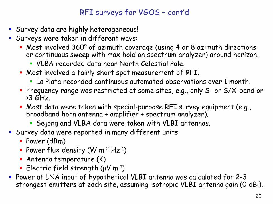
21

Example of La Plata survey results

22

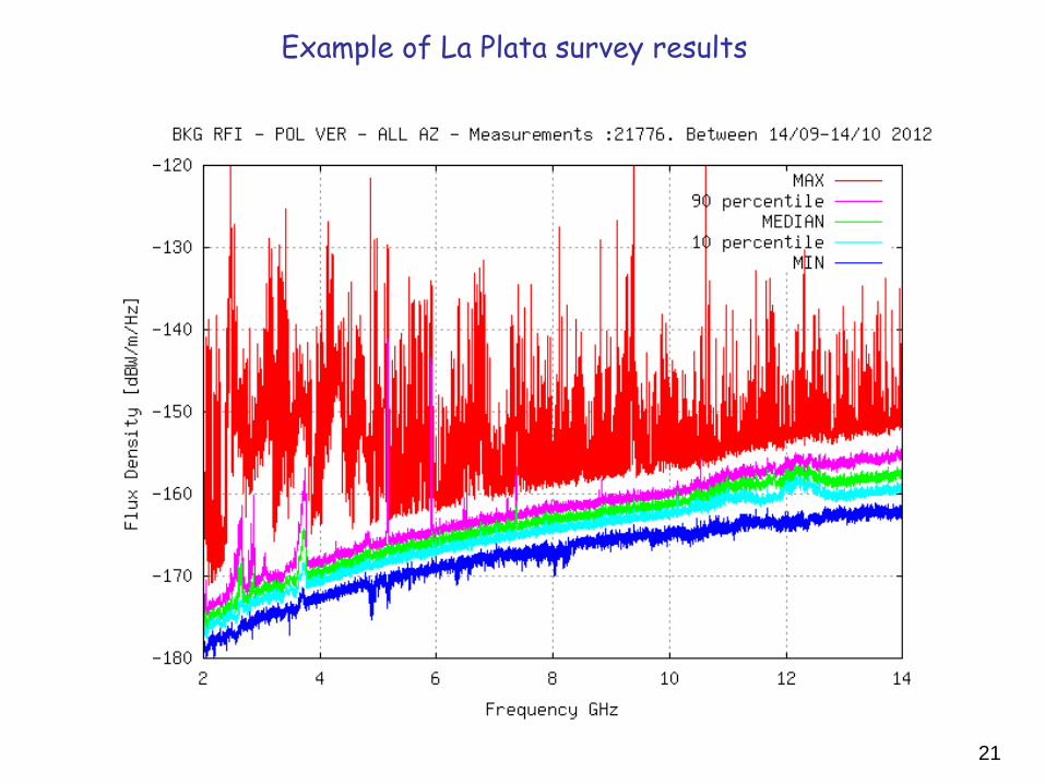
RFI power calculated for VLBI antenna from RFI survey data: 1-15 GHz

23

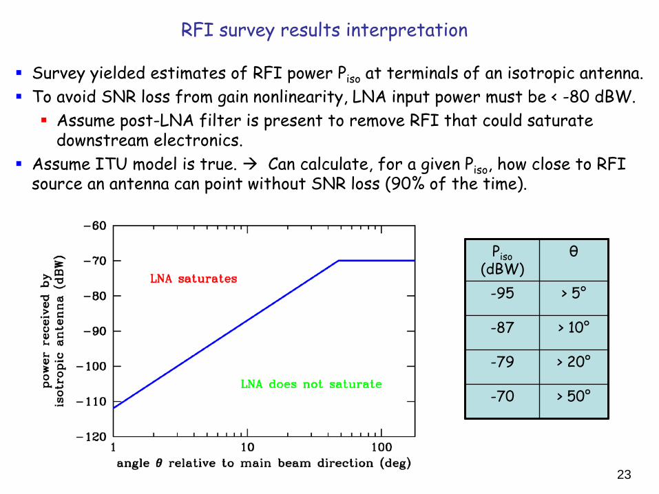
RFI survey results interpretation

Survey yielded estimates of RFI power Piso at terminals of an isotropic antenna. To avoid SNR loss from gain nonlinearity, LNA input power must be < -80 dBW. Assume post-LNA filter is present to remove RFI that could saturate

downstream electronics. Assume ITU model is true. Can calculate, for a given Piso, how close to RFI

source an antenna can point without SNR loss (90% of the time).

Piso (dBW)

θ

-95 > 5°

-87 > 10°

-79 > 20°

-70 > 50°

24

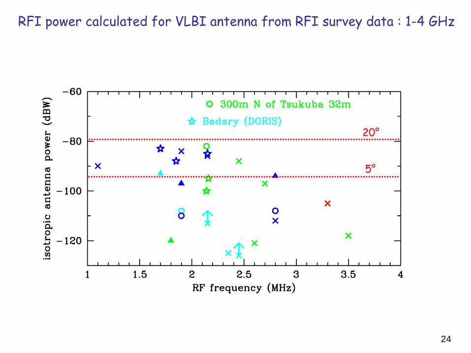
RFI power calculated for VLBI antenna from RFI survey data : 1-4 GHz

20°

5°

RFI Sources, Identification, Mitigation (Part 2)

Mamoru Sekido/NICT

1 An Example of Serious RFI

1.1 Symptom

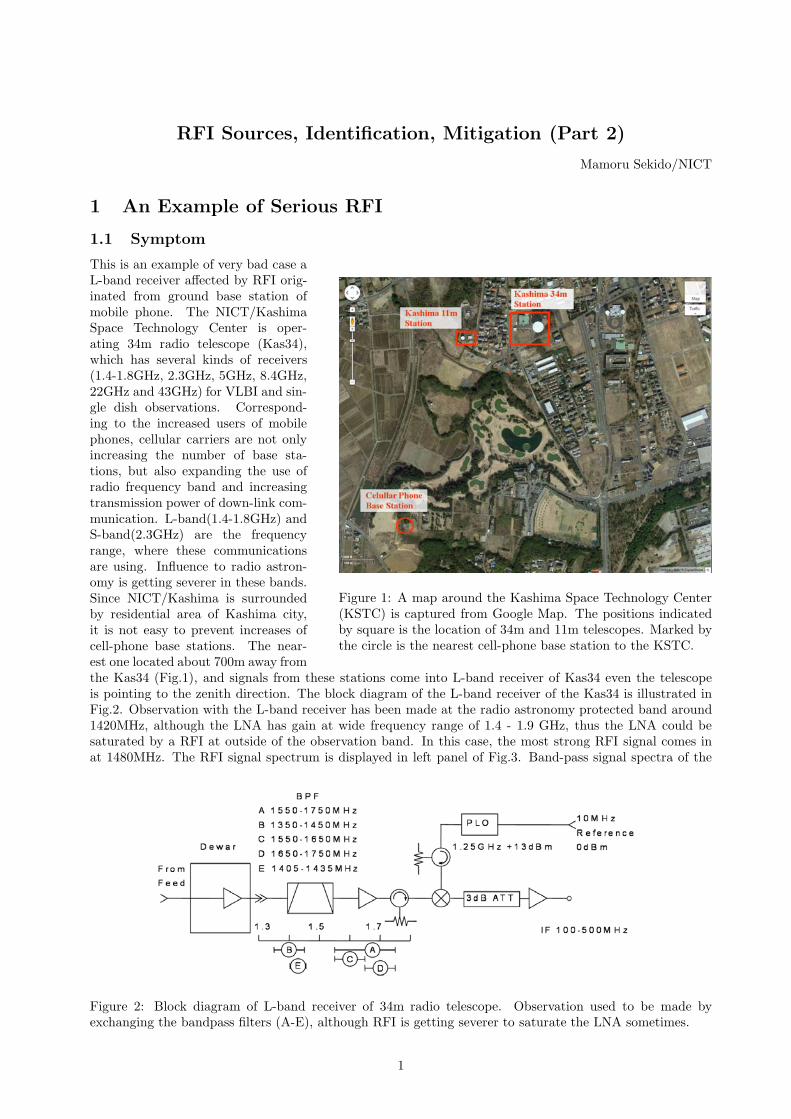
Figure 1: A map around the Kashima Space Technology Center(KSTC) is captured from Google Map. The positions indicatedby square is the location of 34m and 11m telescopes. Marked bythe circle is the nearest cell-phone base station to the KSTC.

This is an example of very bad case aL-band receiver affected by RFI orig-inated from ground base station ofmobile phone. The NICT/KashimaSpace Technology Center is oper-ating 34m radio telescope (Kas34),which has several kinds of receivers(1.4-1.8GHz, 2.3GHz, 5GHz, 8.4GHz,22GHz and 43GHz) for VLBI and sin-gle dish observations. Correspond-ing to the increased users of mobilephones, cellular carriers are not onlyincreasing the number of base sta-tions, but also expanding the use ofradio frequency band and increasingtransmission power of down-link com-munication. L-band(1.4-1.8GHz) andS-band(2.3GHz) are the frequencyrange, where these communicationsare using. Influence to radio astron-omy is getting severer in these bands.Since NICT/Kashima is surroundedby residential area of Kashima city,it is not easy to prevent increases ofcell-phone base stations. The near-est one located about 700m away fromthe Kas34 (Fig.1), and signals from these stations come into L-band receiver of Kas34 even the telescopeis pointing to the zenith direction. The block diagram of the L-band receiver of the Kas34 is illustrated inFig.2. Observation with the L-band receiver has been made at the radio astronomy protected band around1420MHz, although the LNA has gain at wide frequency range of 1.4 - 1.9 GHz, thus the LNA could besaturated by a RFI at outside of the observation band. In this case, the most strong RFI signal comes inat 1480MHz. The RFI signal spectrum is displayed in left panel of Fig.3. Band-pass signal spectra of the

Figure 2: Block diagram of L-band receiver of 34m radio telescope. Observation used to be made byexchanging the bandpass filters (A-E), although RFI is getting severer to saturate the LNA sometimes.

1

L-band RHCP

-100

-95

-90

-85

-80

-75

-70

1.39 1.4 1.41 1.42 1.43 1.44 1.45

Pos

t-L

NA

Out

(dB

m)/

200k

Hz

Freq. (GHz)

Az=180 deg.Az=190 deg.Az=200 deg.Az=210 deg.Az=220 deg.Az=230 deg.Az=240 deg.Az=250 deg.Az=260 deg.

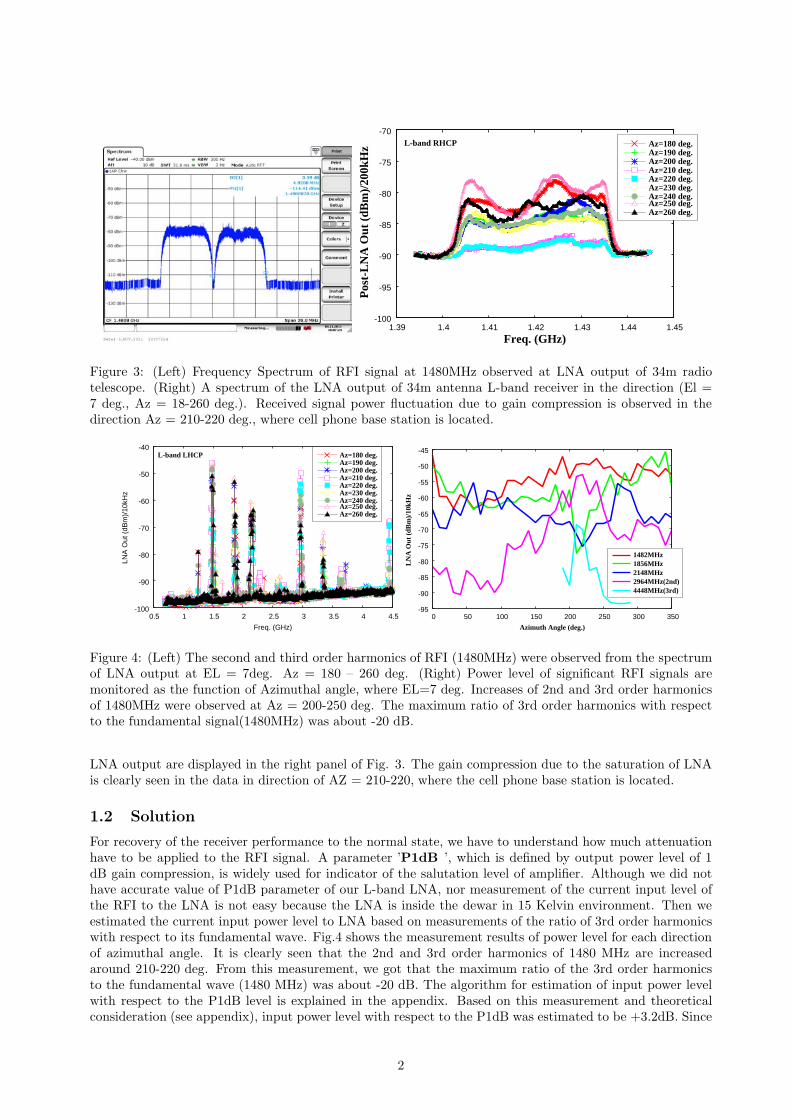
Figure 3: (Left) Frequency Spectrum of RFI signal at 1480MHz observed at LNA output of 34m radiotelescope. (Right) A spectrum of the LNA output of 34m antenna L-band receiver in the direction (El =7 deg., Az = 18-260 deg.). Received signal power fluctuation due to gain compression is observed in thedirection Az = 210-220 deg., where cell phone base station is located.

-100

-90

-80

-70

-60

-50

-40

0.5 1 1.5 2 2.5 3 3.5 4 4.5

LNA

Out

(dB

m)/

10kH

z

Freq. (GHz)

L-band LHCP Az=180 deg.Az=190 deg.Az=200 deg.Az=210 deg.Az=220 deg.Az=230 deg.Az=240 deg.Az=250 deg.Az=260 deg.

-95

-90

-85

-80

-75

-70

-65

-60

-55

-50

-45

0 50 100 150 200 250 300 350

LN

A O

ut (

dBm

)/10

kHz

Azimuth Angle (deg.)

2148MHz2964MHz(2nd)4448MHz(3rd)

1482MHz1856MHz

Figure 4: (Left) The second and third order harmonics of RFI (1480MHz) were observed from the spectrumof LNA output at EL = 7deg. Az = 180 – 260 deg. (Right) Power level of significant RFI signals aremonitored as the function of Azimuthal angle, where EL=7 deg. Increases of 2nd and 3rd order harmonicsof 1480MHz were observed at Az = 200-250 deg. The maximum ratio of 3rd order harmonics with respectto the fundamental signal(1480MHz) was about -20 dB.

LNA output are displayed in the right panel of Fig. 3. The gain compression due to the saturation of LNAis clearly seen in the data in direction of AZ = 210-220, where the cell phone base station is located.

1.2 Solution

For recovery of the receiver performance to the normal state, we have to understand how much attenuationhave to be applied to the RFI signal. A parameter ’P1dB ’, which is defined by output power level of 1dB gain compression, is widely used for indicator of the salutation level of amplifier. Although we did nothave accurate value of P1dB parameter of our L-band LNA, nor measurement of the current input level ofthe RFI to the LNA is not easy because the LNA is inside the dewar in 15 Kelvin environment. Then weestimated the current input power level to LNA based on measurements of the ratio of 3rd order harmonicswith respect to its fundamental wave. Fig.4 shows the measurement results of power level for each directionof azimuthal angle. It is clearly seen that the 2nd and 3rd order harmonics of 1480 MHz are increasedaround 210-220 deg. From this measurement, we got that the maximum ratio of the 3rd order harmonicsto the fundamental wave (1480 MHz) was about -20 dB. The algorithm for estimation of input power levelwith respect to the P1dB level is explained in the appendix. Based on this measurement and theoreticalconsideration (see appendix), input power level with respect to the P1dB was estimated to be +3.2dB. Since

2

linear amplifier usually have to be used less than -10 dB from P1dB power level of the amplifier, requirementof the RFI attenuation is estimated to be more than 13.2 dB (=3.2 dB + 10 dB).

Since the frequency of the RFI signal at 1480MHz is out of the protected frequency band assigned forradio astronomy, we had no legal right to claim to the cell phone company, but thought a communicationchannel to the company at a radio frequency regulation committee meeting, I could make appointment andwent to base station management division of the company. After explanation of the evidence of receiversaturation due to RFI and negotiation with them, we could agreed that the company will bear the expensesof installation of cryogenic filter in front of the LNA to prevent the saturation. The installation of cryogenicfilter and recovery of the L-band receiver is expected to be made by the end of this year.

2 RFI Survey for development of wide-band VLBI System

2.1 Motivation

We are upgrading the MARBLE 1.5m/1.6m diameter antennas to wide-band (VLBI2010 compatible) VLBIsystem. The MARBLE antennas are originally developed for baseline calibration/validation for GNSS re-ceivers under the collaboration with Geographical Survey Institute (GSI) of Japan. S/X-band receivershave been installed in these antennas, though it designed with future extension to wide-band (VLBI2010)specification in mind. Then we have made a RFI survey to check the feasibility of wide-band observationand location of RFI signal, before modification of the MARBLE to wide-band system.

VLBI is relatively robust to the RFI, because local RFI signals are independent each other and it willdiminish in cross correlation processing, as far as it is not strong to overload the receiver system. HoweverRFI signal originated from communication use are usually strong enough with respect to the power level ofradio astronomy observation. It can easily overload the dynamic range of the cascaded amplifiers from frontend to the recording system. Table 1 shows an example of signal power level and gain of a radio telescope.Because of large gain about 90 dB and limited dynamic range, receiver system could be saturated by strongRFI signal in the observation band.

Especially, due to wide observation frequency band of VLBI2010 specification, the receiver is more vul-nerable to RFI and higher P1dB performance is required for the amplifiers. Measurements of RFI signalpower level with respect to that of receiver noise is useful.

Table 1: An example of signal power level and gain of a typical radio telescope.Typical Signal level at LNA input. 100 Kelvin

1.38e-18 mW/Hz(signal level in 1Hz Band width) -179 dBm/Hz

(signal level in 500MHz Band width) -91 dBm/500MHzAmplifier Gain 90 dB

Typical Sampler input level 0 dBmDynamic range of a 8bit A/D sampler (8 bit = 256 levels) 24 dB

2.2 Receiver system and its noise temperature used for the RFI survey.

Portable wide-band receiver (2-18GHz), which was developed in the project “Statistical approach for weakradiation power measurement in radio frequency (SIRIUS)” was used in the radio environment survey. TheSIRIUS receiver has been sometimes suffered from very strong interference below 3 GHz band, then wedecided to introduce high-pass filter (HPF:Fc=3.5GHz) in front of LNA. Therefore This report does notinclude the RFI information below 3 GHz.

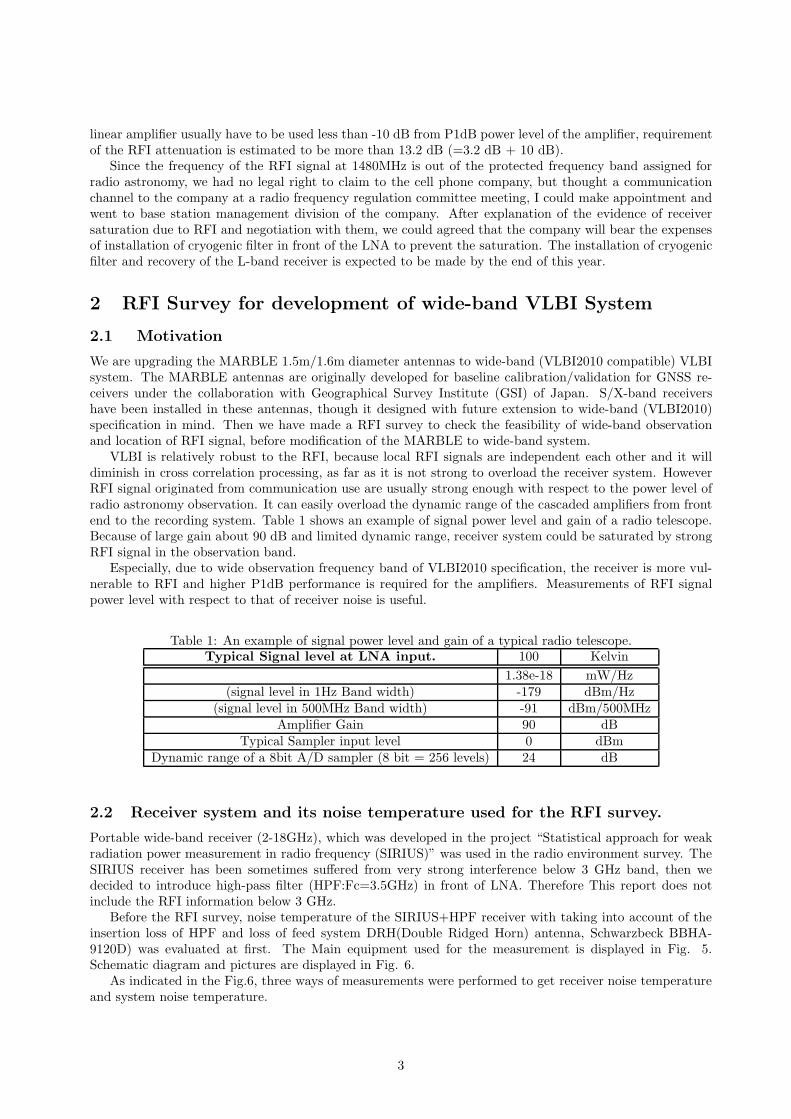
Before the RFI survey, noise temperature of the SIRIUS+HPF receiver with taking into account of theinsertion loss of HPF and loss of feed system DRH(Double Ridged Horn) antenna, Schwarzbeck BBHA-9120D) was evaluated at first. The Main equipment used for the measurement is displayed in Fig. 5.Schematic diagram and pictures are displayed in Fig. 6.

As indicated in the Fig.6, three ways of measurements were performed to get receiver noise temperatureand system noise temperature.

3

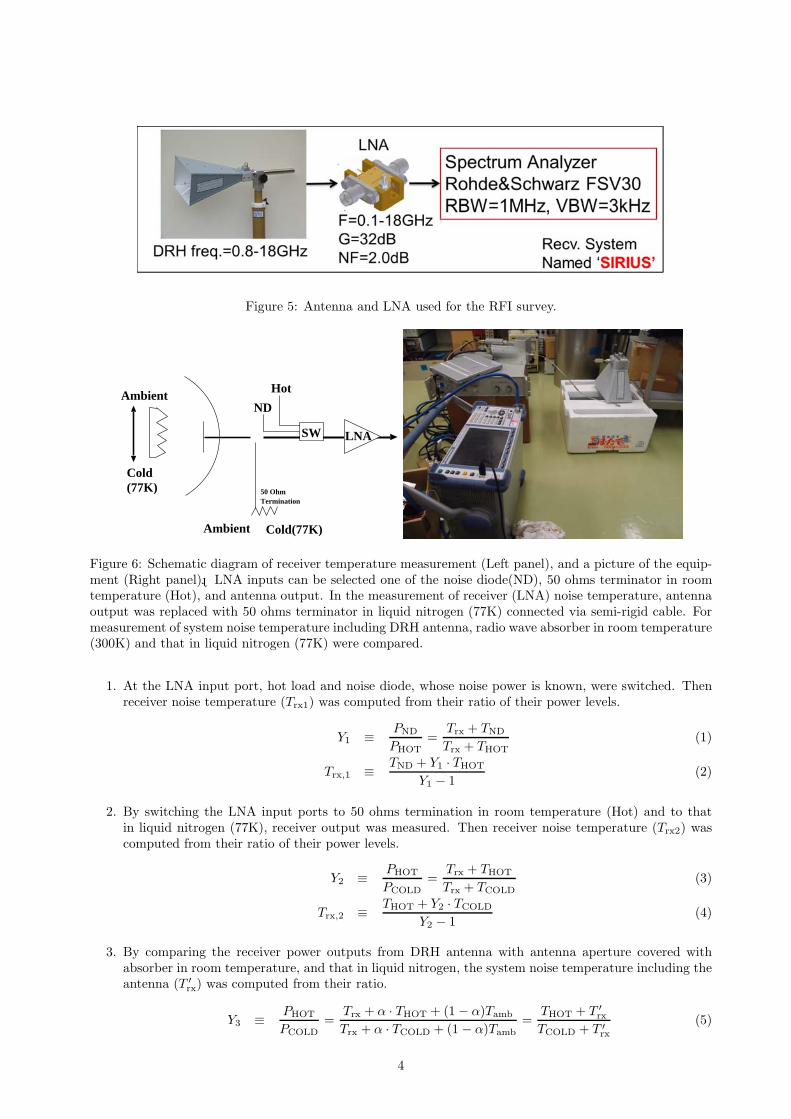
Figure 5: Antenna and LNA used for the RFI survey.

Ambient

Cold(77K)

Hot

ND

Cold(77K)

50 OhmTermination

Ambient

LNASW

Figure 6: Schematic diagram of receiver temperature measurement (Left panel), and a picture of the equip-ment (Right panel)。LNA inputs can be selected one of the noise diode(ND), 50 ohms terminator in roomtemperature (Hot), and antenna output. In the measurement of receiver (LNA) noise temperature, antennaoutput was replaced with 50 ohms terminator in liquid nitrogen (77K) connected via semi-rigid cable. Formeasurement of system noise temperature including DRH antenna, radio wave absorber in room temperature(300K) and that in liquid nitrogen (77K) were compared.

1. At the LNA input port, hot load and noise diode, whose noise power is known, were switched. Thenreceiver noise temperature (Trx1) was computed from their ratio of their power levels.

Y1 ≡ PND

PHOT=

Trx + TND

Trx + THOT(1)

Trx,1 ≡ TND + Y1 · THOT

Y1 − 1(2)

2. By switching the LNA input ports to 50 ohms termination in room temperature (Hot) and to thatin liquid nitrogen (77K), receiver output was measured. Then receiver noise temperature (Trx2) wascomputed from their ratio of their power levels.

Y2 ≡ PHOT

PCOLD=

Trx + THOT

Trx + TCOLD(3)

Trx,2 ≡ THOT + Y2 · TCOLD

Y2 − 1(4)

3. By comparing the receiver power outputs from DRH antenna with antenna aperture covered withabsorber in room temperature, and that in liquid nitrogen, the system noise temperature including theantenna (T ′

rx) was computed from their ratio.

Y3 ≡ PHOT

PCOLD=

Trx + α · THOT + (1 − α)Tamb

Trx + α · TCOLD + (1 − α)Tamb=

THOT + T ′rx

TCOLD + T ′rx

(5)

4

T ′rx ≡ THOT + Y3 · TCOLD

Y3 − 1(6)

where, α indicate the loss factor due to the HPF and the DRH antenna. We assumed ambient tem-perature Tamb is the same with temperature of hot load Tamb � THOT.

T ′rx in equation (6) is system temperature including the antenna. Signal transmission loss α in front of LNA

contributes to the increase of receiver temperature 1/α times as

T ′rx =

(1 − α)Tamb + Trx

α, (7)

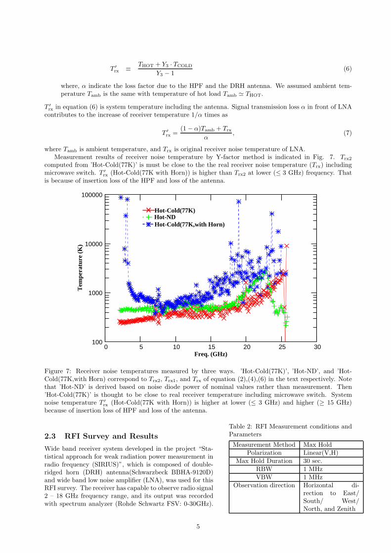
where Tamb is ambient temperature, and Trx is original receiver noise temperature of LNA.Measurement results of receiver noise temperature by Y-factor method is indicated in Fig. 7. Trx2

computed from ’Hot-Cold(77K)’ is must be close to the the real receiver noise temperature (Trx) includingmicrowave switch. T ′

rx (Hot-Cold(77K with Horn)) is higher than Trx2 at lower (≤ 3 GHz) frequency. Thatis because of insertion loss of the HPF and loss of the antenna.

100

1000

10000

100000

0 5 10 15 20 25 30

Tem

pera

ture

(K

)

Freq. (GHz)

Hot-NDHot-Cold(77K)

Hot-Cold(77K,with Horn)

Figure 7: Receiver noise temperatures measured by three ways. ’Hot-Cold(77K)’, ’Hot-ND’, and ’Hot-Cold(77K,with Horn) correspond to Trx2, Trx1, and Trx of equation (2),(4),(6) in the text respectively. Notethat ’Hot-ND’ is derived based on noise diode power of nominal values rather than measurement. Then’Hot-Cold(77K)’ is thought to be close to real receiver temperature including microwave switch. Systemnoise temperature T ′

rx (Hot-Cold(77K with Horn)) is higher at lower (≤ 3 GHz) and higher (≥ 15 GHz)because of insertion loss of HPF and loss of the antenna.

2.3 RFI Survey and Results

Table 2: RFI Measurement conditions andParameters

Measurement Method Max HoldPolarization Linear(V,H)

Max Hold Duration 30 sec.RBW 1 MHzVBW 1 MHz

Observation direction Horizontal di-rection to East/South/ West/North, and Zenith

Wide band receiver system developed in the project “Sta-tistical approach for weak radiation power measurement inradio frequency (SIRIUS)”, which is composed of double-ridged horn (DRH) antenna(Schwarzbeck BBHA-9120D)and wide band low noise amplifier (LNA), was used for thisRFI survey. The receiver has capable to observe radio signal2 – 18 GHz frequency range, and its output was recordedwith spectrum analyzer (Rohde Schwartz FSV: 0-30GHz).

5

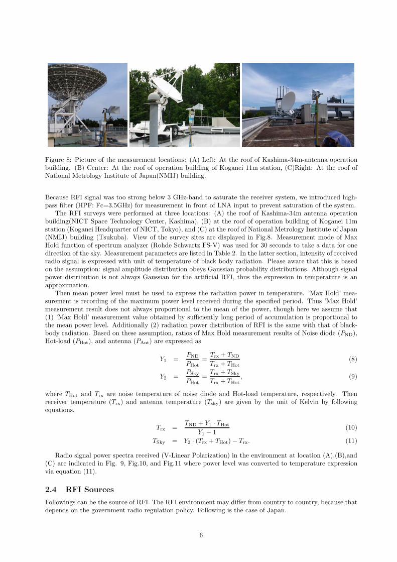
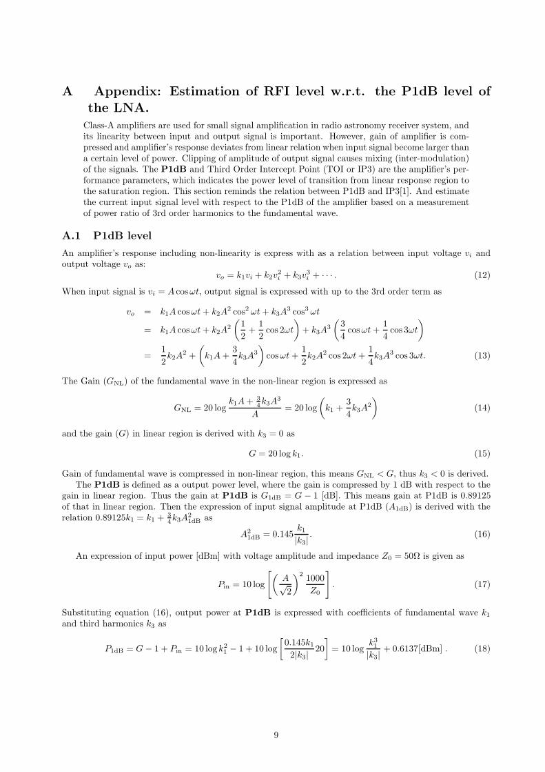
Figure 8: Picture of the measurement locations: (A) Left: At the roof of Kashima-34m-antenna operationbuilding. (B) Center: At the roof of operation building of Koganei 11m station, (C)Right: At the roof ofNational Metrology Institute of Japan(NMIJ) building.

Because RFI signal was too strong below 3 GHz-band to saturate the receiver system, we introduced high-pass filter (HPF: Fc=3.5GHz) for measurement in front of LNA input to prevent saturation of the system.

The RFI surveys were performed at three locations: (A) the roof of Kashima-34m antenna operationbuilding(NICT Space Technology Center, Kashima), (B) at the roof of operation building of Koganei 11mstation (Koganei Headquarter of NICT, Tokyo), and (C) at the roof of National Metrology Institute of Japan(NMIJ) building (Tsukuba). View of the survey sites are displayed in Fig.8. Measurement mode of MaxHold function of spectrum analyzer (Rohde Schwartz FS-V) was used for 30 seconds to take a data for onedirection of the sky. Measurement parameters are listed in Table 2. In the latter section, intensity of receivedradio signal is expressed with unit of temperature of black body radiation. Please aware that this is basedon the assumption: signal amplitude distribution obeys Gaussian probability distributions. Although signalpower distribution is not always Gaussian for the artificial RFI, thus the expression in temperature is anapproximation.

Then mean power level must be used to express the radiation power in temperature. ’Max Hold’ mea-surement is recording of the maximum power level received during the specified period. Thus ’Max Hold’measurement result does not always proportional to the mean of the power, though here we assume that(1) ’Max Hold’ measurement value obtained by sufficiently long period of accumulation is proportional tothe mean power level. Additionally (2) radiation power distribution of RFI is the same with that of black-body radiation. Based on these assumption, ratios of Max Hold measurement results of Noise diode (PND),Hot-load (PHot), and antenna (PAnt) are expressed as

Y1 =PND

PHot=

Trx + TND

Trx + THot(8)

Y2 =PSky

PHot=

Trx + TSky

Trx + THot, (9)

where THot and Trx are noise temperature of noise diode and Hot-load temperature, respectively. Thenreceiver temperature (Trx) and antenna temperature (Tsky) are given by the unit of Kelvin by followingequations.

Trx =TND + Y1 · THot

Y1 − 1(10)

TSky = Y2 · (Trx + THot) − Trx. (11)

Radio signal power spectra received (V-Linear Polarization) in the environment at location (A),(B),and(C) are indicated in Fig. 9, Fig.10, and Fig.11 where power level was converted to temperature expressionvia equation (11).

2.4 RFI Sources

Followings can be the source of RFI. The RFI environment may differ from country to country, because thatdepends on the government radio regulation policy. Following is the case of Japan.

6

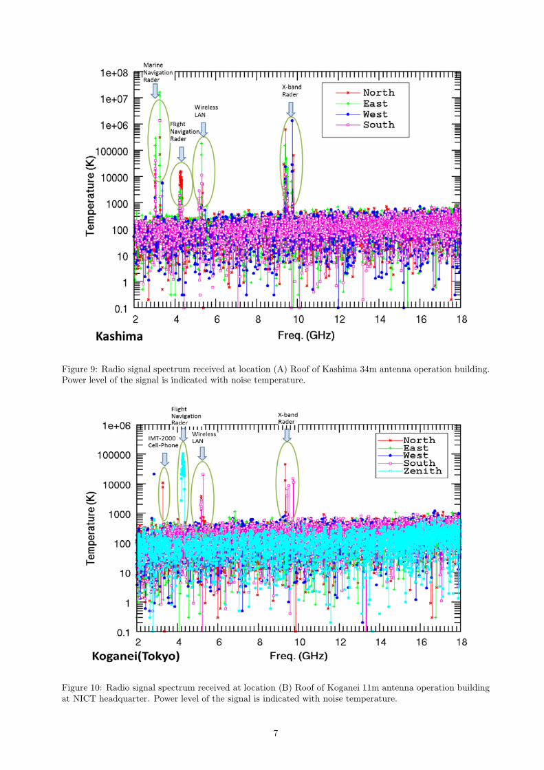
Figure 9: Radio signal spectrum received at location (A) Roof of Kashima 34m antenna operation building.Power level of the signal is indicated with noise temperature.

Figure 10: Radio signal spectrum received at location (B) Roof of Koganei 11m antenna operation buildingat NICT headquarter. Power level of the signal is indicated with noise temperature.

7

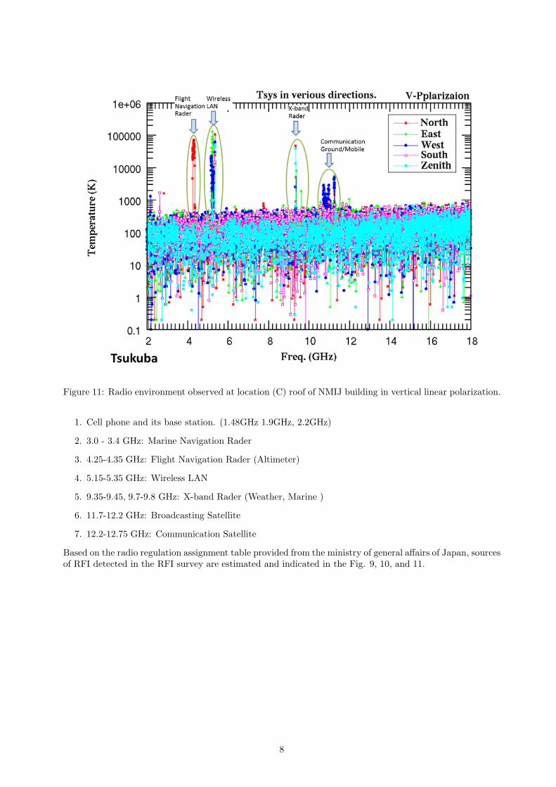
Figure 11: Radio environment observed at location (C) roof of NMIJ building in vertical linear polarization.

1. Cell phone and its base station. (1.48GHz 1.9GHz, 2.2GHz)

2. 3.0 - 3.4 GHz: Marine Navigation Rader

3. 4.25-4.35 GHz: Flight Navigation Rader (Altimeter)

4. 5.15-5.35 GHz: Wireless LAN

5. 9.35-9.45, 9.7-9.8 GHz: X-band Rader (Weather, Marine )

6. 11.7-12.2 GHz: Broadcasting Satellite

7. 12.2-12.75 GHz: Communication Satellite

Based on the radio regulation assignment table provided from the ministry of general affairs of Japan, sourcesof RFI detected in the RFI survey are estimated and indicated in the Fig. 9, 10, and 11.

8

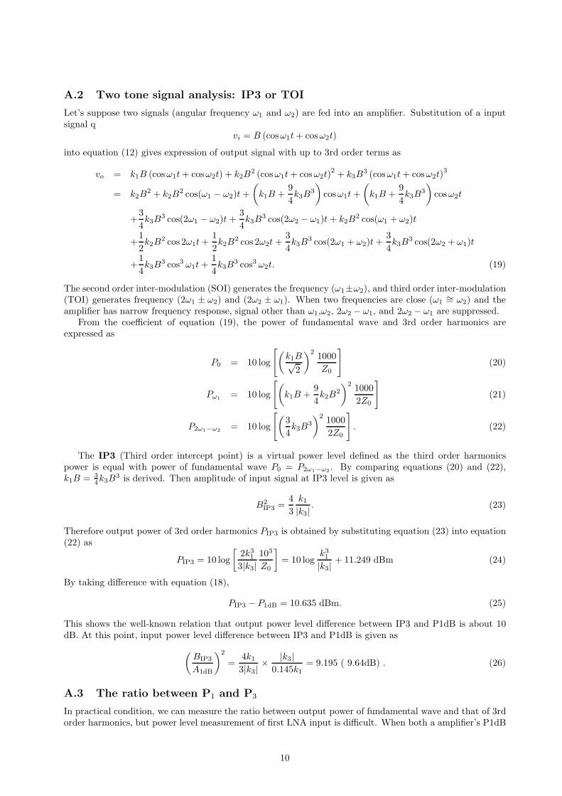
A Appendix: Estimation of RFI level w.r.t. the P1dB level of

the LNA.Class-A amplifiers are used for small signal amplification in radio astronomy receiver system, andits linearity between input and output signal is important. However, gain of amplifier is com-pressed and amplifier’s response deviates from linear relation when input signal become larger thana certain level of power. Clipping of amplitude of output signal causes mixing (inter-modulation)of the signals. The P1dB and Third Order Intercept Point (TOI or IP3) are the amplifier’s per-formance parameters, which indicates the power level of transition from linear response region tothe saturation region. This section reminds the relation between P1dB and IP3[1]. And estimatethe current input signal level with respect to the P1dB of the amplifier based on a measurementof power ratio of 3rd order harmonics to the fundamental wave.

A.1 P1dB level

An amplifier’s response including non-linearity is express with as a relation between input voltage vi andoutput voltage vo as:

vo = k1vi + k2v2i + k3v

3i + · · · . (12)

When input signal is vi = A cosωt, output signal is expressed with up to the 3rd order term as

vo = k1A cosωt + k2A2 cos2 ωt + k3A

3 cos3 ωt

= k1A cosωt + k2A2

(12

+12

cos 2ωt

)+ k3A

3

(34

cosωt +14

cos 3ωt

)

=12k2A

2 +(

k1A +34k3A

3

)cosωt +

12k2A

2 cos 2ωt +14k3A

3 cos 3ωt. (13)

The Gain (GNL) of the fundamental wave in the non-linear region is expressed as

GNL = 20 logk1A + 3

4k3A3

A= 20 log

(k1 +

34k3A

2

)(14)

and the gain (G) in linear region is derived with k3 = 0 as

G = 20 log k1. (15)

Gain of fundamental wave is compressed in non-linear region, this means GNL < G, thus k3 < 0 is derived.The P1dB is defined as a output power level, where the gain is compressed by 1 dB with respect to the

gain in linear region. Thus the gain at P1dB is G1dB = G − 1 [dB]. This means gain at P1dB is 0.89125of that in linear region. Then the expression of input signal amplitude at P1dB (A1dB) is derived with therelation 0.89125k1 = k1 + 3

4k3A21dB as

A21dB = 0.145

k1

|k3| . (16)

An expression of input power [dBm] with voltage amplitude and impedance Z0 = 50Ω is given as

Pin = 10 log

[(A√2

)2 1000Z0

]. (17)

Substituting equation (16), output power at P1dB is expressed with coefficients of fundamental wave k1

and third harmonics k3 as

P1dB = G − 1 + Pin = 10 log k21 − 1 + 10 log

[0.145k1

2|k3| 20]

= 10 logk31

|k3| + 0.6137[dBm] . (18)

9

A.2 Two tone signal analysis: IP3 or TOI

Let’s suppose two signals (angular frequency ω1 and ω2) are fed into an amplifier. Substitution of a inputsignal q

vi = B (cosω1t + cosω2t)

into equation (12) gives expression of output signal with up to 3rd order terms as

vo = k1B (cosω1t + cosω2t) + k2B2 (cosω1t + cosω2t)

2 + k3B3 (cosω1t + cosω2t)

3

= k2B2 + k2B

2 cos(ω1 − ω2)t +(

k1B +94k3B

3

)cosω1t +

(k1B +

94k3B

3

)cosω2t

+34k3B

3 cos(2ω1 − ω2)t +34k3B

3 cos(2ω2 − ω1)t + k2B2 cos(ω1 + ω2)t

+12k2B

2 cos 2ω1t +12k2B

2 cos 2ω2t +34k3B

3 cos(2ω1 + ω2)t +34k3B

3 cos(2ω2 + ω1)t

+14k3B

3 cos3 ω1t +14k3B

3 cos3 ω2t. (19)

The second order inter-modulation (SOI) generates the frequency (ω1±ω2), and third order inter-modulation(TOI) generates frequency (2ω1 ± ω2) and (2ω2 ± ω1). When two frequencies are close (ω1

∼= ω2) and theamplifier has narrow frequency response, signal other than ω1,ω2, 2ω2 − ω1, and 2ω2 − ω1 are suppressed.

From the coefficient of equation (19), the power of fundamental wave and 3rd order harmonics areexpressed as

P0 = 10 log

[(k1B√

2

)2 1000Z0

](20)

Pω1 = 10 log

[(k1B +

94k2B

2

)2 10002Z0

](21)

P2ω1−ω2 = 10 log

[(34k3B

3

)2 10002Z0

]. (22)

The IP3 (Third order intercept point) is a virtual power level defined as the third order harmonicspower is equal with power of fundamental wave P0 = P2ω1−ω2 . By comparing equations (20) and (22),k1B = 3

4k3B3 is derived. Then amplitude of input signal at IP3 level is given as

B2IP3 =

43

k1

|k3| . (23)

Therefore output power of 3rd order harmonics PIP3 is obtained by substituting equation (23) into equation(22) as

PIP3 = 10 log[

2k31

3|k3|103

Z0

]= 10 log

k31

|k3| + 11.249 dBm (24)

By taking difference with equation (18),

PIP3 − P1dB = 10.635 dBm. (25)

This shows the well-known relation that output power level difference between IP3 and P1dB is about 10dB. At this point, input power level difference between IP3 and P1dB is given as

(BIP3

A1dB

)2

=4k1

3|k3| ×|k3|

0.145k1= 9.195 ( 9.64dB) . (26)

A.3 The ratio between P1 and P3

In practical condition, we can measure the ratio between output power of fundamental wave and that of 3rdorder harmonics, but power level measurement of first LNA input is difficult. When both a amplifier’s P1dB

10

level and its input power level is unknown, we have to estimate the current input power level with respectto the P1dB of the amplifier.

When single tone signal is input, the output power ration between fundamental wave and 3rd orderharmonics is expressed with the coefficient of the equation (13) as

R13 ≡ P3

P1=( 1

4k3A3

k1A + 34k3A3

)2

=

( |k3|k1

A2

4 − 3 |k3|k1

A2

)2

(27)

√R13 =

α( AA1dB

)2

4 − 3α( AA1dB

)2, (28)

where α ≡ 0.145 and equation(16) were used. The first equation represent the power ratio and the secondequation express the amplitude ratio with the amplitude of P1dB level. Then the ratio of current inputpower level with respect to the P1dB input level is expressed by

(A

A1dB

)2

=4√

R13

α(1 + 3√

R13). (29)

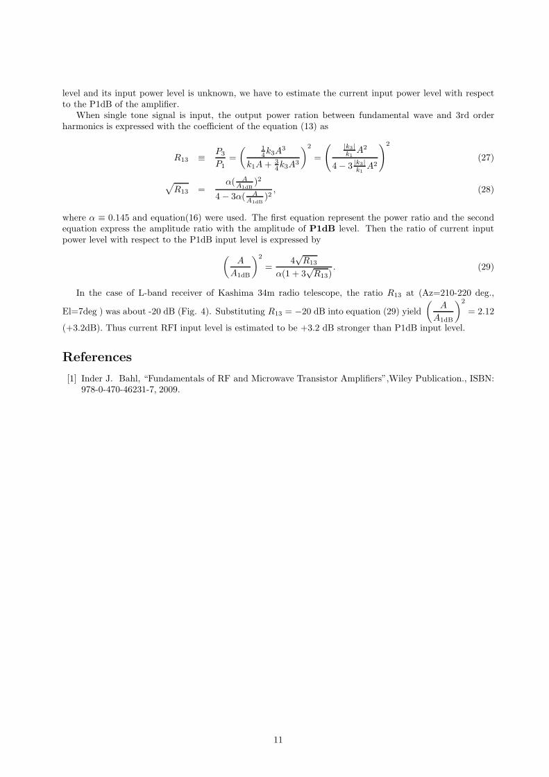
In the case of L-band receiver of Kashima 34m radio telescope, the ratio R13 at (Az=210-220 deg.,

El=7deg ) was about -20 dB (Fig. 4). Substituting R13 = −20 dB into equation (29) yield(

A

A1dB

)2

= 2.12

(+3.2dB). Thus current RFI input level is estimated to be +3.2 dB stronger than P1dB input level.

References

[1] Inder J. Bahl, “Fundamentals of RF and Microwave Transistor Amplifiers”,Wiley Publication., ISBN:978-0-470-46231-7, 2009.

11