RGISTools: Downloading, Customizing, andProcessing Time-Series of Remote Sensing Data in

R

Unai Pérez-GoyaPublic University of Navarre

InaMat Institute

Manuel Montesino-SanMartinPublic University of Navarre

InaMat Institute

Ana F. MilitinoPublic University of Navarre

InaMat Institute

M. Dolores UgartePublic University of Navarre

InaMat Institute

Abstract

There is a large number of data archives and web services offering free access to mul-tispectral satellite imagery. Images from multiple sources are increasingly combined toimprove the spatio-temporal coverage of measurements while achieving more accurate re-sults. Archives and web services differ in their protocols, formats, and data standards,which are barriers to combine datasets. Here, we present RGISTools, an R package to cre-ate time-series of multispectral satellite images from multiple platforms in a harmonizedand standardized way. We first provide an overview of the package functionalities, namelydownloading, customizing, and processing multispectral satellite imagery for a region andtime period of interest as well as a recent statistical method for gap-filling and smooth-ing series of images, called interpolation of the mean anomalies. We further show thecapabilities of the package through a case study that combines Landsat-8 and Sentinel-2satellite optical imagery to estimate the level of a water reservoir in Northern Spain. Weexpect RGISTools to foster research on data fusion and spatio-temporal modelling usingsatellite images from multiple programs.

Keywords: Landsat, MODIS, Sentinel, satellite images, spatio-temporal data, IMA.

1. Introduction

Satellite images represent a valuable data source in large-scale long-term research studies.Landsat, MODIS, and Copernicus are major programs for the acquisition of images of theEarth’s surface supported by the U.S. Geological Survey (USGS), NASA, and the EuropeanSpace Agency (ESA) respectively. Images are freely accessible in large data archives, whichcan be retrieved via web services such as EarthData, NASA Inventory or SciHub. Dataarchives offer long series of records, dating back to 1972 for Landsat, 1999 for MODIS and2013 for Sentinel. Satellite imagery has proven useful for studies in many disciplines, suchas poverty assessments (Jean, Burke, Xie, Davis, Lobell, and Ermon 2016), glacier dynamics(Paul, Winsvold, Kääb, Nagler, and Schwaizer 2016), soil classification (Gomez, Dharumara-

arX

iv:2

002.

0185

9v1

[st

at.C

O]

5 F

eb 2

020

2 RGISTools: Time-Series of Remote Sensing Data in R

jan, Féret, Lagacherie, Ruiz, and Sekhar 2019), distribution of animal species (Swinbourne,Taggart, Swinbourne, Lewis, and Ostendorf 2018), and crop monitoring (Azzari, Jain, andLobell 2017).Missions have strengths and weaknesses regarding the spatial and temporal resolution of theirimagery. The satellite constellation of MODIS acquires images on a daily basis at a moderatespatial resolution (250m). Landsat and Sentinel multispectral constellations capture high-resolution images (15-60m and 10-60m respectively) where locations are revisited roughly ona weekly basis (8 and 5 days). Studies claim the need for a higher spatio-temporal resolutionthan those obtained from single programs (Griffiths, Nendel, and Hostert 2019). Data fusionhas been proposed to counteract inadequate resolutions by blending information at differentlevels, pixel-level (e.g., MODIS and Sentinel), feature-level (e.g., class of land-cover) or thedecision-level (Belgiu and Stein 2019). This is partly possible thanks to improvements inavailability and accessibility of satellite images over the last decade. Some challenges stillremain. Web services and programs work with particular query protocols, file formats, anddata standards. Becoming familiar with the details of every archive can be tedious and timeconsuming. A harmonized single access point and processing software would benefit theresearch community removing complexity and fostering data fusion.R (R Core Team 2019) is an open source software increasingly used for the analysis of satelliteimages, as it enables the application of state-of-the-art statistical methods. There are manyreliable packages to manipulate spatial or spatio-temporal data, such as raster (Hijmans2019) and sf (Pebesma 2018), or to perform spatio-temporal statistical analyses, such as gstat(Pebesma 2004). Packages working with satellite images already exist in R. Few packagesdeal with imagery from several programs, but they are focused on specific tasks of the overallworkflow with satellite images. SkyWatchr (Santacruz and Developers 2017) finds and down-loads Landsat, MODIS, Sentinel, and private company’s imagery but does not support dataprocessing or customization. ASIP (Riyas and Syed 2018) is able to carry out a restrictedset of processing steps for Landsat and Sentinel imagery, such as atmospheric corrections andspectral index computations, leaving uncovered cloud masking or smoothing. Other packageshave greater functionalities but they are specialized in particular programs or data products.For instance, MODIStsp (Busetto and Ranghetti 2016) downloads, mosaics, re-projects, andcomputes spectral indices from MODIS images exclusively. MODIS (Mattiuzzi and Detsch2019) andMODISTools (Tuck, Phillips, Hintzen, Scharlemann, Purvis, and Hudson 2014) alsowork with MODIS imagery but with more restricted functionalities. MODISnow (Signer andTrubilowicz 2016) and modiscloud (Matzke 2013) only access snowcover products and cloudmasks, respectively. Regarding Sentinel-2, the sen2r package (Ranghetti and Busetto 2019) iscapable of finding, downloading, and processing data products just from this satellite mission.The R packages landsat (Goslee 2011), satellite (Nauss, Meyer, Detsch, and Appelhans 2015),and landsat8 (dos Santos 2017) mainly perform radiometric and topographic corrections ofLandsat (or Landsat-8), but they are not able to do the download. Consequently, there is aneed for a comprehensive package that harmonizes the work with different satellite programs.RGISTools (Pérez-Goya, Militino, Ugarte, and Montesino-SanMartin 2019) is conceived inresponse to those needs. The package is a toolbox to work with time-series of satellite imagesfrom Landsat, MODIS, and Sentinel repositories in a standardized way. The functions ofRGISTools allow to build a semiautomatic line of work for downloading, customizing, andprocessing imagery. The download process includes the search and preview of images fora region and period of interest. The customization covers image mosaicking, cropping, and

Unai Pérez-Goya, Manuel Montesino-SanMartin, Ana F. Militino, M. Dolores Ugarte 3

extracting the required bands. Processing functions comprise cloud removal, definition of newvariables, gap filling, and image smoothing. RGISTools is available from the Comprehensive RArchive Network in https://cran.r-project.org/web/packages/RGISTools/index.htmland the Git hub repository in https://github.com/spatialstatisticsupna/RGISTools.The structure of this paper is as follows: Section 2 introduces basic information to handlesatellite images. Section 3 gives an overview of the work sequence with the package. Thissection provides brief descriptions of the aim and inputs of each function. Explanations arecoupled with a MODIS example on using the interpolation of the mean anomalies (IMA)procedure for gap-filling and smoothing images that is available in the package. In Section 4,we present an example that combines Landsat-8 and Sentinel-2 to monitor the water levelsof a reservoir in Northern Spain.

2. Satellite programsThe package focuses on optical imagery, which is the form of satellite information most com-monly used in research. Operational satellite missions concerning with optical measurementsare Landsat-7, Landsat-8, MODIS, and Sentinel-2.

2.1. Data types and structure

Wavelengths and band names

The type and structure of satellite data varies with the mission. Each mission involves oneor several satellites that carry purpose-specific instruments (Table 1). On board instrumentsmeasure the solar radiance in specific bands of the electromagnetic spectrum. For instance,the Terra and Aqua satellites from MODIS carry on-board the moderate resolution imagingspectroradiometer (MODIS). It captures 36 bands in the visible and infrared parts of thespectrum (NASA 2019e). MODIS collects information on a greater number of bands andwith narrower spectral windows than Landsat-7 (8 bands), Landsat-8 (11 bands) (USGS2019b), and Sentinel-2 (12 bands) (ESA 2019h) satellites. Bands are identified by numbers,which are given in sequential order. Similar wavelengths might be labelled with differentnumbers depending on the mission. For instance, the red band (0.673 − 0.695µm) is the band3 in Landsat-7’s imagery, the band 4 in Landsat-8’s and Sentinel-2, and bands 1, 13, and 14in MODIS. Computing remote sensing indices can be problematic due to inconsistencies inthe band names.

Tiling systems

Satellite records are partitioned into scenes that cover portions of the earth’s surface, calledtiles. Tiling systems are conceived to facilitate data processing and sharing. Each missionhas its own tiling system, varying in tile’s size, orientation, and naming conventions. Forexample, MODIS tiles are considerably larger (1200 × 1200 km2 ) than the ones used forLandsat-7 (170×183 km2), Landsat-8 (185×180 km2) or Sentinel-2 (100×100 km2). Satelliteprograms provide keyhole markup language files (KML) with the boundaries of the tiles attheir respective official websites (USGS 2019a; ORNL DAAC 2019; ESA 2019b). Dependingon the mission, one or several tiles can cover the region of interest. In the latter situation,

4 RGISTools: Time-Series of Remote Sensing Data in R

images should be properly merged and cropped.

Data products and processing levels

Sensor features, radiometric, and geometric effects distort satellite images. Corrections arerequired to convert sensor data into surface reflectances. Programs offer several productsdepending on the level of processing being applied. Generally, level-2 products are processedto provide the surface reflectances and they are suitable for most applications. MODISadditionally distinguishes different products depending on the scientific field to which theinformation is targeted (atmospheric, cryogenic, and land products) (NASA 2019d). Basedon the purpose of the satellite imagery, the researcher must select the appropriate productand processing level. During the correction process, images are also geo-referenced. MODISdefines the coordinates of the pixels using the global sinusoidal projection (NASA 2019e),while Landsat and Sentinel use the universal trade mercator (UTM) system under the worldgeodetic system 1984 (WGS84) (USGS 2019b; ESA 2019h). Any fusion between MODIS andLandsat/Sentinel datasets would require to re-project one of two collection of images.

2.2. Sharing protocols and data formats

Web services

Web services represent an interactive mean to access the archives of one or several programs.They offer one or two ways to access the imagery: through a graphic user interface (GUI)or an application programming interface (API). APIs are specially convenient to search anddownload time-series of satellite images programatically. Major existing web services withAPIs are EarthData (NASA 2019a), NASA Inventory (NASA 2019c), and SciHub (ESA2019a). Users can select among several query options and should interpret the response inextensible markup language (XML) or javascript object notation (JSON).

Formats

Pixel values are re-scaled and images are compressed to preserve the information efficientlyand accurately. Satellite programs use different formats and compression methods (see Ta-ble 1). Landsat images are encoded as GTiff and stored as tape archive files (".tar") andGNU compression standards (".gz") (USGS 2019b). MODIS images are shared in hierarchicaldata format (".hdf") (NASA 2019d). Sentinel images are available as raster images usingJPEG2000 format (".jp2") and encapsulated as ".tar.gz" files (ESA 2019b). Images must beextracted and once imported, pixel values representing surface reflectance are usually scaledbetween 0 and 10000. However, actual ranges are generally larger as a result of the correctionalgorithms. In MOD09GA, surface reflectance goes from -100 to 16000. Pixel values shouldbe truncated and re-scaled for some applications.The aim of RGISTools is to centralize the information, standardize, and automate satelliteimagery retrival, customization, and processing. The following sections describe how to usethe package to obtain a complete and ready-to-use time-series of remote sensing data.

3. RGISTools overview

Unai Pérez-Goya, Manuel Montesino-SanMartin, Ana F. Militino, M. Dolores Ugarte 5

Program Landsat MODIS SentinelMission Landsat-7 Landsat-8 - Sentinel-2Satellite Landsat-7 Landsat-8 Terra Aqua A BSensor ET+ TIRS/OLI MODIS MODIS MSI MSINo. Bands 8 8 36 36 12 12Time Revisit (days) 16 16 1 1 10 10Resolution (m) 30-60 15-30 250 250 10-60 10-60Format GTiff GTiff HDF-EOS HDF-EOS JP2 JP2

Table 1: Major satellite missions devoted to multi-spectral images and details about theirdatasets.

The RGISTools package works with multiple sources of information and, for this reason, thefunctions are grouped into 5 categories depending on the mission they focus on. Functionsbegin with one of the following prefixes:

• ls, mod, and sen involve Landsat, MODIS and Sentinel imagery respectively. Morespecifically, ls7 and ls8 are restricted to Landsat-7 and Landsat-8 missions.

• gen can be applied to images from any mission.

• var compute widespread remote sensing indices.

The package implements a variety of procedures related to downloading, customizing, andprocessing satellite images. A suffix in the function’s name indicates its purpose. The mainfunctionalities of RGISTools are introduced in the following sections along with an exam-ple analysing the spatio-temporal evolution of the Normalized Difference Vegetation Index(NDVI) (Rouse Jr 1972).RGISTools downloads and works with satellite imagery locally on your computer. Then, asa memory-saving strategy, most functions deal with images externally to R. The workflow isdesigned to delay the data loading in the R environment until the end of the customization.At this point, the relevant data have been transformed to meet the particular needs of theanalysis. As a result, rather than R objects, downloading and customizing functions take afile path as an input (src argument) and generate GTiffs and folders in a given directory(AppRoot argument) as an output. Functions print a message when completing their taskto help remembering the output location. A clear hierarchical structure of folders and anappropriate file management are key to work successfully with RGISTools.The NDVI example requires in total 0.92 Giga Bytes (GB) of memory space. It takes nearly5 minutes to run from top to bottom in an intel(R) Core(TM) i7-6700 CPU @3.40 GHz andan internet connection speed of 310 Mbps. In case of insufficient memory space, we providelinks throughout the next sections to download the resulting files. After data processing, thefile size decreases from a maximum of 198 MB to a minimum of 3 MB.

3.1. Retrieving satellite imagery

Retrieving satellite imagery involves three steps; searching, previewing, and downloadingscenes for a specific time-period and region of interest (ROI). Some of these steps require

6 RGISTools: Time-Series of Remote Sensing Data in R

valid credentials from EarthData (NASA 2019b) and SciHub (Copernicus 2019) web services,which can be acquired after registration in their respective websites.

Searching

The first step in retrieving satellite images is to search the scenes available for a particularROI and time window. Search results provide valuable information on the number of avail-able images, the dates they were captured, or the tiles they belong to. The lsSearch(),modSearch(), and senSearch() functions require as inputs the name of the data product,the time interval, and the ROI.A data product is a collection of images with certain bands and processing level. Productsare identified by short-names, which can be found in Landsat, MODIS, and Sentinel websitesand product guides (NASA 2019d; ESA 2019g). The spatio-temporal domain under analysisis specified through a time interval (dates) and a location (region). The time span is definedby a vector of ‘Date’ class objects and the ROI can be any spatial object in R (‘Spatial*’,‘sf’, or ‘raster’).In the following, we search multispectral images of the surface reflectance (level-2) of opticalbands captured by the Terra satellite (“MOD09GA” product) between the 2nd and 9th ofAugust 2018. The ROI is the Navarre province located in Northern Spain. The border of thisregion is represented in ex.navarre as a ‘SimpleFeature’ with a ‘MULTIPOLYGON’ geometry:

R> library("RGISTools")R> wdir <- tempdir()

R> data("ex.navarre")R> sres <- modSearch(product = "MOD09GA",+ dates = as.Date("2018-08-02") + seq(0 , 7, 1),+ region = ex.navarre)

Previewing

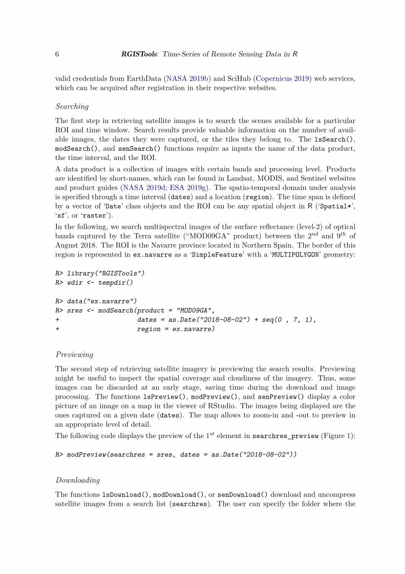
The second step of retrieving satellite imagery is previewing the search results. Previewingmight be useful to inspect the spatial coverage and cloudiness of the imagery. Thus, someimages can be discarded at an early stage, saving time during the download and imageprocessing. The functions lsPreview(), modPreview(), and senPreview() display a colorpicture of an image on a map in the viewer of RStudio. The images being displayed are theones captured on a given date (dates). The map allows to zoom-in and -out to preview inan appropriate level of detail.The following code displays the preview of the 1st element in searchres_preview (Figure 1):

R> modPreview(searchres = sres, dates = as.Date("2018-08-02"))

Downloading

The functions lsDownload(), modDownload(), or senDownload() download and uncompresssatellite images from a search list (searchres). The user can specify the folder where the

Unai Pérez-Goya, Manuel Montesino-SanMartin, Ana F. Militino, M. Dolores Ugarte 7

Figure 1: A preview of the 1st image of the “MOD09GA” time-series. The image corre-sponds to the “h:17v:4” tile from MODIS, which covers the region of Navarre (ex.navarre)in Northern Spain. The image was captured on August 2nd, 2018 by the Terra satellite.

imagery will be placed using the AppRoot argument or images will be saved in the currentworking directory otherwise.The function downloads and saves the satellite images in their original format in a folderautomatically created under AppRoot. If the proper flag is active (e.g., extract.tif = TRUEin MODIS), the function decompresses and transforms the imagery to GTiff. The uncom-pressed images are saved in another folder also generated automatically in AppRoot. If onlyfew bands of the spectrum are needed, the argument bFilter allows to specify which bandsshould be transformed.Below, we download and uncompress the previously found time-series of images (sres). Asmentioned earlier, the imagery will be used to compute the NDVI index (see Section 3.2),so the red (“B01”) and near-infrared (“B02”) bands must be extracted. We also require thequality band (“state”) to be able to remove the pixels covered by clouds.To run the next code, replace the <USERNAME> and <PASSWORD> with the credentials acquiredat NASA (2019b). Images are saved in the wdir.mod.download directory (i.e., ./Modis/MOD09GA)inside a temporary directory:

R> wdir.mod <- file.path(wdir, "Modis")

R> wdir.mod <- file.path(wdir, "Modis")R> wdir.mod.download <- file.path(wdir.mod, "MOD09GA")R> modDownload(searchres = sres,+ AppRoot = wdir.mod.download,+ extract.tif = TRUE,+ bFilter = c("B01", "B02", "state"),+ username = "<USERNAME>",

8 RGISTools: Time-Series of Remote Sensing Data in R

+ password = "<PASSWORD>",+ overwrite = TRUE)

The preview might not be necessary when further filtering is not required or there is no interestin exploring the tiles covering the ROI. In these situations, the functions lsDownSearch(),modDownSearch(), and senDownSearch() can search, download, and uncompress the time-series of images at once. An example follows:

R> modDownSearch(product = "MOD09GA",+ dates = as.Date("2018-08-02") + seq(0, 7 , 1),+ region = ex.navarre,+ AppRoot = wdir,+ extract.tif = TRUE,+ bFilter = c("B01", "B02", "state"),+ username = "<USERNAME>",+ password = "<PASSWORD>")

The code above takes few minutes to run and requires 0.913 GB of space in the disk. Theuser can download the results as GTiff files (0.198 GB) from the reference Vermonte (2019a).Please, unzip the file and save it in the ./Modis folder to continue with the example.

3.2. Customizing satellite imagery

Here, customizing satellite images refers to mosaicking, cropping, and computing remotesensing indices.

Mosaicking and cropping

Mosaicking means joining satellite images captured on the same date and from different tilesto obtain a single scene covering the ROI. Cropping is the removal of pixels outside the spatialbounding box that encapsulates the ROI. Both tasks are meant to rearrange the dataset andpreserve the relevant information only. Mosaicking and cropping functions are named after thecorresponding satellite mission and the keyword Mosaic (i.e., lsMosaic(), modMosaic(), andsenMosaic()). These functions require the path to the folder that contains the uncompressedimage files (src). When provided, the function crops the image around the bounding box ofthe spatial object (‘Spatial*’, ‘sf’, or ‘raster’) that is passed through the argument region.Mosaic functions use by default the Geospatial Data Abstraction Library (contributors 2019)through the the sf package interface (Pebesma 2018). If gutils is set to FALSE, the functionborrows the mosaic functionalities from the raster package (Hijmans 2019). However, GDALis more computationally efficiently than raster. The results are saved in a new folder in theAppRoot directory named as the out.name argument.Mosaicking and cropping the imagery from previous examples is shown below. Croppedimages are saved into a folder called Navarre under the wdir.mod directory (i.e., ./Modis):

R> wdir.mod.tif <- file.path(wdir.mod,"MOD09GA","tif")R> modMosaic(src = wdir.mod.tif,+ region = ex.navarre,

Unai Pérez-Goya, Manuel Montesino-SanMartin, Ana F. Militino, M. Dolores Ugarte 9

+ out.name = "Navarre",+ gutils = TRUE,+ AppRoot = wdir.mod)

The MODIS tile covering Navarre is unique (“h17:v4”), so in our example, modMosaic() justcrops the images around the bounding box of ex.navarre.Mosaicking and cropping takes few seconds to run with gutils = TRUE. The size of theoverall outcoming images is 3.72 MB. To ensure that the rest of the analysis is reproducible,the results are available at the reference Vermonte (2019b). No more files are providedthrough links hereinafter for the MODIS example, as we consider that the size of the dataset is manageable, and the computational times for the rest of the example are sensible.

Computing remote sensing indicesA common use of multispectral images is the computation of remote sensing indices. Theseare mathematical expressions combining the reflectance of several bands of the spectrumto highlight the phenomenon under analysis. The package includes pre-built functions thatdefine widespread remote sensing indices (i.e., varNDVI(), varEVI(), varNBR(), etc.). TheNormalized Difference Vegetation Index (NDVI) (Rouse Jr 1972) is a commonly used indexto monitor green vegetation. It uses the red and near-infrared wavelengths (Didan, Munoz,Solano, and Huete 2015) due to the high levels of absorption and reflection in these wave-lengths by plants.The functions lsFolderToVar(), modFolderToVar(), and senFolderToVar() apply the varfunctions over a time-series of multispectral satellite images. The family of FolderToVarfunctions requires as inputs the path to the folder that stores the mosaicked images (srcargument) and the function that computes the remote sensing index (fun argument). Theoutputs are saved in a folder named after the remote sensing index, in the AppRoot directory.For instance, the following code calculates a daily series of NDVIs from the images mosaickedin the previous section. The resulting images are saved in wdir.mod (i.e., ./Modis/NDVI):

R> wdir.mod.mosaic <- file.path(wdir.mod, "Navarre")R> modFolderToVar(src = wdir.mod.mosaic,+ fun = varNDVI,+ AppRoot = wdir.mod)

The generated data can be loaded in R using the stack() function from the raster package(Hijmans 2019) (Figure 2). Due to errors in some pixel values, results of the NDVI may yieldresults outside the usual -1 and 1 range (Rouse Jr 1972). These artifacts can be removed withthe function clamp() from raster (Hijmans 2019) as follows:

R> wdir.mod.ndvis <- file.path(wdir.mod, "NDVI")R> files.mod.ndvi <- list.files(wdir.mod.ndvis, full.names = TRUE)R> imgs.mod.raw <- raster::stack(files.mod.ndvi)R> imgs.mod.ndvi <- raster::clamp(imgs.mod.raw, lower = -1, upper = 1)

RGISTools includes the function genPlotGIS() to display satellite imagery. genPlotGIS()is a wrapper function of tmap (Tennekes 2018) with options and layers configured to easilydisplay the spatial information dealt within RGISTools:

10 RGISTools: Time-Series of Remote Sensing Data in R

2°W 1°W

42°N

43°N

2°W 1°W

42°N

43°N

2°W 1°W

42°N

43°N

2°W 1°W

42°N

43°N

2°W 1°W

42°N

43°N

2°W 1°W

42°N

43°N

2°W 1°W

42°N

43°N

2°W 1°W

42°N

43°N

0 10 20 30 40 km 0 10 20 30 40 km 0 10 20 30 40 km 0 10 20 30 40 km

0 10 20 30 40 km 0 10 20 30 40 km 0 10 20 30 40 km 0 10 20 30 40 km

NDVI_2018214 NDVI_2018215 NDVI_2018216 NDVI_2018217

NDVI_2018218 NDVI_2018219 NDVI_2018220 NDVI_2018221

1

0.9

0.8

0.7

0.6

0.5

0.4

0.3

0.2

0.1

0

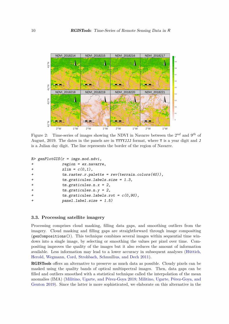
Figure 2: Time-series of images showing the NDVI in Navarre between the 2nd and 9th ofAugust, 2019. The dates in the panels are in YYYYJJJ format, where Y is a year digit and Jis a Julian day digit. The line represents the border of the region of Navarre.

R> genPlotGIS(r = imgs.mod.ndvi,+ region = ex.navarre,+ zlim = c(0,1),+ tm.raster.r.palette = rev(terrain.colors(40)),+ tm.graticules.labels.size = 1.3,+ tm.graticules.n.x = 2,+ tm.graticules.n.y = 2,+ tm.graticules.labels.rot = c(0,90),+ panel.label.size = 1.5)

3.3. Processing satellite imagery

Processing comprises cloud masking, filling data gaps, and smoothing outliers from theimagery. Cloud masking and filling gaps are straightforward through image compositing(genCompositions()). This technique combines several images within sequential time win-dows into a single image, by selecting or smoothing the values per pixel over time. Com-positing improves the quality of the images but it also reduces the amount of informationavailable. Less information may lead to a lower accuracy in subsequent analyses (Hüttich,Herold, Wegmann, Cord, Strohbach, Schmullius, and Dech 2011).RGISTools offers an alternative to preserve as much data as possible. Cloudy pixels can bemasked using the quality bands of optical multispectral images. Then, data gaps can befilled and outliers smoothed with a statistical technique called the interpolation of the meananomalies (IMA) (Militino, Ugarte, and Pérez-Goya 2018; Militino, Ugarte, Pérez-Goya, andGenton 2019). Since the latter is more sophisticated, we elaborate on this alternative in the

Unai Pérez-Goya, Manuel Montesino-SanMartin, Ana F. Militino, M. Dolores Ugarte 11

following paragraphs.

Cloud masking

Satellite programs apply their own methodology to determine the pixels covered by clouds(Zhu, Qiu, He, and Deng 2018). The results are saved in the quality bands of level-2 products,together with other information affecting the quality of the surface reflectance estimates (seee.g., Vermote 2015). The functions lsCloudMask(), modCloudMask(), and senCloudMask()interpret the quality bands in each program and save time-series of cloud masks to disk. Inthese masks, clear-sky and cloudy pixels are represented by 1s and NAs respectively.The following code extracts the cloud masks for the MODIS time-series. The masks areplaced by modCloudMask() in a new folder defined by out.name in the wdir directory (i.e.,./Modis/mod_cldmask):

R> modCloudMask(src = wdir.mod.mosaic,+ out.name = "mod_cldmask",+ AppRoot = wdir.mod)

Masks are saved as GTiff files, which can be imported into R. In the following chunk of code,the files with the cloud masks are listed and loaded as a ‘stack’. As cloud masks containcategorical values, they must be converted into ‘factor’ with the function ratify():

R> wdir.mod.cld <- file.path(wdir.mod, "mod_cldmask")R> files.mod.cld <- list.files(wdir.mod.cld, full.names = TRUE)R> imgs.mod.cld <- raster::stack(files.mod.cld)R> imgs.mod.cld <- raster::stack(lapply(as.list(imgs.mod.cld), ratify))

Cloud masks could be on a coarser scale (here, 1 × 1 km2) than the multispectral images(0.5 × 0.5 km2). Masks can be resampled with the projectRaster() function to obtainrasters at the same resolution as the multispectral images. Since the masks are categoricalvalues (1s for clear-sky and NAs for cloudy pixels), the resampling is carried out with thenearest neighbor method. Cloud masks can be applied to the NDVI images as follows:

R> imgs.mod.masks <- raster::projectRaster(imgs.mod.cld,+ imgs.mod.ndvi[[1]],+ method = "ngb")R> imgs.mod.ndvimks <- imgs.mod.masks * imgs.mod.ndviR> names(imgs.mod.ndvimks) <- names(imgs.mod.ndvi)

Gap-filling and smoothing

Cloud removal or sensor failures can lead to data gaps in the time-series of satellite images.Additionally, noise from aerosols, dust, and sensor measurement errors can reduce the qualityof the remotely sensed data. Many gap-filling and smoothing approaches have been devel-oped to mitigate these issues (Shen, Li, Cheng, Zeng, Yang, Li, and Zhang 2015). Amongthem, there is the IMA procedure, which was developed by Militino et al. (2018, 2019).

12 RGISTools: Time-Series of Remote Sensing Data in R

RGISTools implements a generic version of the algorithm in the genSmoothingIMA() andgenSmoothingCovIMA() functions.IMA borrows information from a temporal neighborhood of the image to be filled or smoothed(target image henceforth). The neighborhood extends around the images that are assumedto be similar to the target image. Two parameters confine the size of the neighborhood;nDays, that is, the number of days before and after the capturing date of the target image,and nYears, which is the number of previous and subsequent years. For instance, if nDays= 1 and nYears = 1, the neighborhood is built from images within a period of 1 day beforeand after the target image plus images from the same days of the year but in the previousand subsequent years. IMA uses incomplete neighborhoods in case some images do not exist.Then, the function conducts the following steps:

1. Obtain the average image of the neighboring images.

2. Subtract the average image from the target image to obtain an image of anomalies.

3. Screen out the anomalies outside a range of percentiles (e.g., 0.05-0.95).

4. Aggregate the anomaly image into a coarser resolution using the mean or median (funargument) and an aggregation factor (fact argument). For instance, fun = ’mean’and fact = 4 averages sets of 4 pixels into a single pixel.

5. Interpolate the aggregated image of anomalies using thin-plate splines from the fieldspackage (Nychka, Furrer, Paige, and Sain 2017).

6. Predict the target image in the original resolution adding the interpolated anomaliesand the average image.

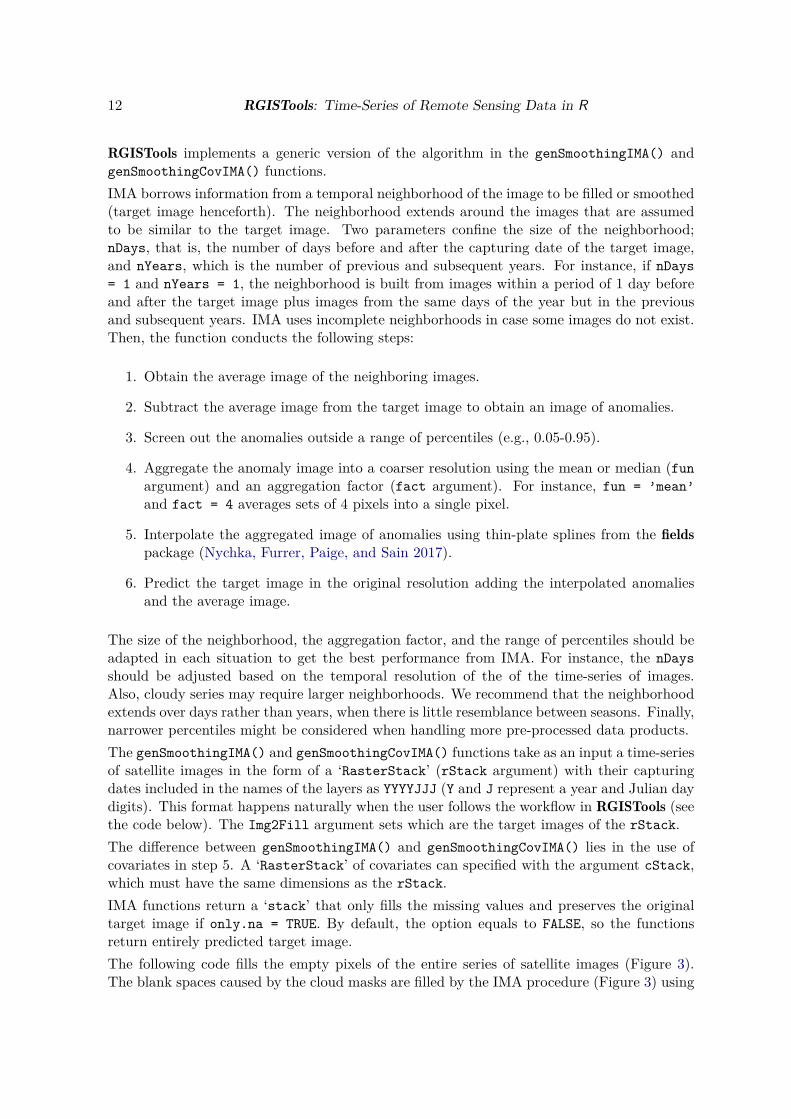
The size of the neighborhood, the aggregation factor, and the range of percentiles should beadapted in each situation to get the best performance from IMA. For instance, the nDaysshould be adjusted based on the temporal resolution of the of the time-series of images.Also, cloudy series may require larger neighborhoods. We recommend that the neighborhoodextends over days rather than years, when there is little resemblance between seasons. Finally,narrower percentiles might be considered when handling more pre-processed data products.The genSmoothingIMA() and genSmoothingCovIMA() functions take as an input a time-seriesof satellite images in the form of a ‘RasterStack’ (rStack argument) with their capturingdates included in the names of the layers as YYYYJJJ (Y and J represent a year and Julian daydigits). This format happens naturally when the user follows the workflow in RGISTools (seethe code below). The Img2Fill argument sets which are the target images of the rStack.The difference between genSmoothingIMA() and genSmoothingCovIMA() lies in the use ofcovariates in step 5. A ‘RasterStack’ of covariates can specified with the argument cStack,which must have the same dimensions as the rStack.IMA functions return a ‘stack’ that only fills the missing values and preserves the originaltarget image if only.na = TRUE. By default, the option equals to FALSE, so the functionsreturn entirely predicted target image.The following code fills the empty pixels of the entire series of satellite images (Figure 3).The blank spaces caused by the cloud masks are filled by the IMA procedure (Figure 3) using

Unai Pérez-Goya, Manuel Montesino-SanMartin, Ana F. Militino, M. Dolores Ugarte 13

2°W 1°W

42°N

43°N

2°W 1°W

42°N

43°N

2°W 1°W

42°N

43°N

2°W 1°W

42°N

43°N

2°W 1°W

42°N

43°N

2°W 1°W

42°N

43°N

2°W 1°W

42°N

43°N

2°W 1°W

42°N

43°N

0 10 20 30 40 km 0 10 20 30 40 km 0 10 20 30 40 km 0 10 20 30 40 km

0 10 20 30 40 km 0 10 20 30 40 km 0 10 20 30 40 km 0 10 20 30 40 km

NDVI_2018214 NDVI_2018215 NDVI_2018216 NDVI_2018217

NDVI_2018218 NDVI_2018219 NDVI_2018220 NDVI_2018221

1

0.9

0.8

0.71

0.61

0.51

0.41

0.32

0.22

0.12

0.02

Figure 3: Reconstructed NDVI from cloud-masked images using the interpolation of themean anomalies (IMA) procedure. The scenes cover August 2nd −9th, 2019 (2018220-2018221in YYYYJJJ format).

a neighborhood of 8 days from the same year of the target image. IMA does not guaranteethat the prediction of the NDVI stays in the [-1,1] range, so the results must be truncatedwith the clamp() function from raster. To look at the dataset for our ROI alone, we maskthe pixels outside Navarre with mask():

R> imgs.mod.imaraw <- genSmoothingIMA(rStack = imgs.mod.ndvimks,+ Img2Fill = 1:nlayers(imgs.mod.ndvimks),+ nDays = 8,+ nYears = 1,+ aFilter = c(0.05, 0.95),+ fact = 8)R> imgs.mod.imaclamp <- raster::clamp(imgs.mod.imaraw, lower = -1, upper = 1)R> ex.mod.navarre <- sf::st_transform(ex.navarre,+ crs = projection(imgs.mod.imaclamp))R> imgs.mod.imanavarre <- raster::mask(imgs.mod.imaclamp, ex.mod.navarre)R> genPlotGIS(imgs.mod.imanavarre,+ region = ex.mod.navarre,+ tm.graticules.labels.size = 1.3,+ tm.graticules.n.x = 2,+ tm.graticules.n.y = 2,+ tm.graticules.labels.rot = c(0,90),+ panel.label.size = 1.5,+ tm.raster.r.palette = rev(terrain.colors(40)))

IMA can be used with datasets retrieved or loaded with other packages. Other classes, such

14 RGISTools: Time-Series of Remote Sensing Data in R

as ‘stars’ or ‘satellite’ objects, can be easily coerced into ‘RasterStack’. To facilitate theinteroperability of IMA with other packages, the function allows to pass the capturing datesof the imagery as a vector of ‘Dates’ class objects through the argument r.dates.

4. Working exampleIn this section, we present a case study that combines Landsat-8 and Sentinel-2 imagery tomonitor the water level of a reservoir in Northern Spain. Section 4.1 defines the ROI andintroduces the auxiliary data required for this exercise (topographic data and water levelobservations). Section 4.2 retrieves Landsat-8 and Sentinel-2 images for the period and theregion of analysis. In Section 4.3, the satellite imagery is customized (cropping and computinga remote sensing index) to detect the surface of the water body. Section 4.4 translates theflooded area into water levels with the aid of the topographic map. Finally, results arecontrasted with the in situ measurements.The working example takes 81.24 GB of memory space and the overall running time is less than3 hours. However, it is divided into shorter parts, whose results are available via downloadablefiles. Thus, the code in each part can be reproduced independently from each other. Thedemand of time and memory space decreases throughout the example, being the maximum80.5 GB and 2.2 hours to run Section 4.2 and the minimum 0.07 GB and nearly 3 seconds tocomplete Section 4.3.

4.1. Region of interest

We examine the Itoiz reservoir, which is located in Northern Spain within the region ofNavarre. The dam was built to collect the waters from the Irati river. The reservoir islocated northeast the village of Aoiz, in the foothills of the Pyrenees. The pond extends over1100 ha and has a capacity of 418 hm3. The reservoir became fully operational in 2006.In the following code, the spatial domain of the water body is defined using the sf pack-age (Pebesma 2018). The area is delimited by a ‘bbox’ with the minimum and maximumlongitude-latitude coordinates. The ‘bbox’ is transformed into a ‘sfc’ class object to createa rectangular polygon, and then turned into an ‘sf’ object:

R> roi.bbox <- sf::st_bbox(c(xmin = -1.40,+ xmax = -1.30,+ ymin = 42.79,+ ymax = 42.88),+ crs = 4326)R> roi.sfc <- sf::st_as_sfc(roi.bbox)R> roi.sf <- sf::st_as_sf(roi.sfc)

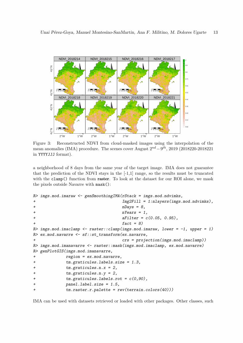
The water level refers to the elevation reached by the pond’s shoreline, which can be derivedby superimposing the flooded area and a topographic map. A contour map is freely availableat the local government’s website (Government of Navarre 2019), which was interpolated toa 10 meter resolution map applying the inverse distance weighting (IDW) method from gstat(Pebesma 2004). The elevation map (Figure 4) was named as altimetry.itoiz and savedas a ‘RasterLayer’ into an “RData” file.

Unai Pérez-Goya, Manuel Montesino-SanMartin, Ana F. Militino, M. Dolores Ugarte 15

632,000 634,000 636,000 638,0004,740,000

4,745,000

4,750,000

N

0.0 0.5 1.0 1.5 2.0 2.5 km

Z480 to 500500 to 520520 to 540540 to 560560 to 580580 to 600600 to 620620 to 640640 to 660

Figure 4: Elevation map of the basin of the Itoiz reservoir. The elevation (Z) is measuredin meters above sea level (m.a.s.l.). The map was derived from freely available informationprovided via online by the local administration (Government of Navarre 2019).

The map (0.77 MB) is available at the link provided in the reference Government of Navarreand Saih (2019). The file should be downloaded, unzipped, and placed in the wdir directory.Then, the map can be loaded as:

R> wdir.topo <- file.path(wdir, "aux_info", "topography_Itoiz.RData")R> load(wdir.topo)

As mentioned earlier, the estimates will be compared with in situ observations. Water levelsare measured on a daily basis at the dam wall and made publicly available at the AutomaticHydrological Information System of the Ebro River Basin Authority (Ebro River Basin Au-thority 2019). The file is available at the reference provided above and can be loaded asfollows:

R> wdir.levels <- file.path(wdir, "aux_info", "level_itoiz.csv")R> obs.itoiz <- read.csv(wdir.levels, colClasses = c("Date", "numeric"))

4.2. Retrieving satellite imagery

Finding a time-seriesThe functions lsSearch() and senSearch() scan the Landsat and Sentinel-2 repositories tofind those scenes that match the requested data product (product), time interval (dates),and ROI (region = roi.sf). In this working example, we want to track the water levelsfrom mid summer 2018 to mid spring 2019 (i.e., dates = as.Date("2018-07-01") + seq(0,304, 1)), as this is the time of the season that water storage varies the most.Landsat and Sentinel search functions allow to filter the results by cloud coverage. Discardingcloudy images at an early stage can save space in the disk and processing time. The cloud

16 RGISTools: Time-Series of Remote Sensing Data in R

coverage filter can be set with the cloudCover argument, indicating the lower and upperpercentages of the pixels of an image being covered by clouds. The view of the reservoir islikely obstructed by clouds during winter, since it is located in a mountainous area. Hence,we restrict our search to images with a cloud coverage below 80% (cloudCover = c(0,80)).We use the surface reflectance product to perform our analysis, i.e., imagery that has beenatmospherically corrected (level-2). Landsat only provides immediate access to level-1 prod-ucts (product = "LANDSAT_8_C1"), so in order to obtain the level-2 product, we must searchlevel-1 images first and then, at the time of downloading, request their correction to theEarth Resources Observation and Science (EROS) Center through their Science ProcessingArchitecture (ESPA) (Jenkerson 2019):

R> library("RGISTools")R> sres.ls8 <- lsSearch(product = "LANDSAT_8_C1",+ dates = as.Date("2018-07-01") + seq(0, 304, 1),+ region = roi.sf,+ cloudCover = c(0,80),+ username = "<USERNAME>",+ password = "<PASSWORD>")

The function lsSearch() returns a ‘data.frame’ with the images that were found as rowsand their metadata details as columns. Regarding Sentinel, surface reflectance images areavailable from the Sentinel-2 mission with the product “S2MSI2A” (Sentinel-2 MultiSpectrallevel-2A):

R> sres.sn2 <- senSearch(platform = "Sentinel-2",+ product = "S2MSI2A",+ dates = as.Date("2018-07-01") + seq(0, 304, 1),+ region = roi.sf,+ cloudCover = c(0,80),+ username = "<USERNAME>",+ password = "<PASSWORD>")

Note that both lsSearch() and senSearch() require the log-in credentials in contrast tomodSearch(). The credentials are required to access the information available at EarthEx-plorer and SciHub. Replace the <USERNAME> and <PASSWORD> with your own credentials aftersigning up for both web services (NASA 2019b; Copernicus 2019). The senSearch() functionreturns a vector of URLs.

Downloading

The lsDownload() and senDownload() functions retrieve the time-series of satellite imagesfound in the previous section (sres.ls8 and sres.sn2). Be aware that downloading satelliteimages can be time-consuming and requires enough storage space in the disk (2.2 hoursand 80.5 GB). In case of insufficient memory space, you can skip this section and downloadthe results concerning Landsat-8 (7.66 GB) (EROS ESPA 2019a) and Sentinel-2 (12 GB)images(ESA 2019c) or get the results from subsequent milestones.

Unai Pérez-Goya, Manuel Montesino-SanMartin, Ana F. Militino, M. Dolores Ugarte 17

As mentioned earlier, Landsat-8 images must be atmospherically corrected by EROS. By set-ting lvl = 2, lsDownload() makes a request to ESPA to process the list of level-1 images(sres.ls8) and gets the corresponding level-2 from their response. To distinguish this re-quest from previous ones, the petition should be named using the l2rqname argument. Thedownloaded files are directly saved in the ./Landsat8/raw directory. For our purpose, weonly require the green (“band3”) and near infra-red (“band5”) bands from the multispectralimages to compute the NDWI (McFeeters 1996) and the quality (“pixel_qa”) band to analysethe cloud coverage. The bFilter argument allows to extract specific bands, which are thensaved as GTiffs in the ./Landsat8/untar directory. Once the transformation is completed,the original files could be removed to free up memory space by adding raw.rm = TRUE:

R> wdir.ls8 <- file.path(wdir, "Landsat8")

R> lsDownload(searchres = sres.ls8,+ lvl = 2,+ untar = TRUE,+ bFilter = list("band3", "band5", "pixel_qa"),+ username = "<USERNAME>",+ password = "<PASSWORD>",+ l2rqname = "<REQUESTNAME>",+ raw.rm = TRUE,+ AppRoot = wdir)

Similarly, senDownload() downloads and uncompressed images from Sentinel. In Sentinel-2,the bands 3 and 8 correspond to green a near infra-red wavelengths. Both bands are availableat a maximum resolution of 10m, so we refer to them as “B03_10m” and “B08_10m”. Thecloud coverage is captured by the cloud probability band (CLDPRB), which is available ata maximum resolution of 20 m (“CLDPRB_20m”). In the code that follows, the functiondownloads the file in ./Sentinel2/raw directory, extracts the bands, and saves them in the./Sentinel2/unzip directory. To clear memory space, we specify raw.rm = TRUE to deletethe original files in ./Sentinel2/raw:

R> wdir.sn2 <- file.path(wdir, "Sentinel2")

R> senDownload(searchres = sres.sn2,+ unzip = TRUE,+ bFilter = list("B03_10m", "B08_10m", "CLDPRB_20m"),+ username = "<USERNAME>",+ password = "<PASSWORD>",+ raw.rm = TRUE,+ AppRoot = wdir.sn2)

4.3. Customizing satellite imagery

Mosaicking and cropping

18 RGISTools: Time-Series of Remote Sensing Data in R

Due to the size of the ROI, it is computationally and memory efficient to remove the pixelsoutside roi.sf. The next code applies lsMosaic() and senMosaic() to the images saved in./Landsat8/untar and ./Sentinel2/unzip. The results are placed in two folders created au-tomatically by the Mosaic functions; ./Landsat8/ls8_itoiz and ./Sentinel2/sn2_itoiz):

R> wdir.ls8.untar <- file.path(wdir.ls8, "untar")R> lsMosaic(src = wdir.ls8.untar,+ region = roi.sf,+ out.name = "ls8_itoiz",+ gutils = TRUE,+ AppRoot = wdir.ls8)R> wdir.sn2.unzip <- file.path(wdir.sn2, "unzip")R> senMosaic(src = wdir.sn2.unzip,+ region = roi.sf,+ out.name = "sn2_itoiz",+ gutils = TRUE,+ AppRoot = wdir.sn2)

The original tiles are not required for the subsequent steps of the analysis, so we remove themto clear memory space as follows:

R> unlink(wdir.ls8.untar, recursive = TRUE)R> unlink(wdir.sn2.unzip, recursive = TRUE)

Cropping the series of images requires roughly 15 minutes and the results occupy 280 MBof memory in the hard disk. If needed, the results are available at EROS ESPA (2019b)for Landsat-8 and at ESA (2019d) for Sentinel-2. The following steps require the files tobe uncompressed and saved in two folders called ./Landsat8 and ./Sentinel2 in the wdirdirectory.

Cloud mask filtering

Clouds in the area may hamper the identification of the water-body shoreline. Here, weinspect the cloudiness at the reservoir by extracting and analyzing the cloud masks. ThelsCloudMask() and senCloudMask() functions interpret the information about the presenceof clouds from the quality bands. The location of these quality bands must be indicatedthrough the src argument. The generated cloud masks are saved in AppRoot directory, in anew folder named as the out.name argument:

R> wdir.ls8.mosaic <- file.path(wdir.ls8, "ls8_itoiz")R> lsCloudMask(src = wdir.ls8.mosaic,+ out.name = "ls8_cldmask",+ AppRoot = wdir.ls8)R> wdir.sn2.mosaic <- file.path(wdir.sn2, "sn2_itoiz")R> senCloudMask(src = wdir.sn2.mosaic,+ out.name = "sn2_cldmask",+ AppRoot = wdir.sn2)

Unai Pérez-Goya, Manuel Montesino-SanMartin, Ana F. Militino, M. Dolores Ugarte 19

The quality bands are translated into cloud masks in few seconds for both series of imagesand the outputs take 2.14 MB of memory. Results are available in EROS ESPA (2019c) and(ESA 2019e) for Landsat-8 and Sentinel-2 respectively. Download the files and unzip themat ./Landsat8 and ./Sentinel2.In the following, we load the cloud masks to conduct further analyses:

R> wdir.ls8.cld <- file.path(wdir.ls8, "ls8_cldmask")R> wdir.sn2.cld <- file.path(wdir.sn2, "sn2_cldmask")R> wdir.all.cld <- list(wdir.ls8.cld, wdir.sn2.cld)R> files.cld.msk <- lapply(wdir.all.cld, list.files, full.names = TRUE)R> imgs.cld.msk <- lapply(files.cld.msk, raster::stack)R> names(imgs.cld.msk) <- c("ls8", "sn2")

The next code finds the dates in which the cloud coverage remained below a threshold at theItoiz reservoir. The threshold was set to 30% for Landsat-8 and 0.1% for Sentinel-2 images.These thresholds were decided through visual inspection of the images and the cloud masks.Landsat-8 has a higher threshold than Sentinel-2 due to missclassified water pixels as cloudsby the Landsat-8 algorithms:

R> cld.coverage <- lapply(imgs.cld.msk,+ function(x){colSums(is.na(getValues(x)))/ncell(x)})R> names(cld.coverage) <- c("ls8", "sn2")R> ls8.clr.dates <- genGetDates(names(imgs.cld.msk$ls8))[cld.coverage$ls8 < 0.30]R> sn2.clr.dates <- genGetDates(names(imgs.cld.msk$sn2))[cld.coverage$sn2 < 0.001]

Both ls8.clr.dates and sn2.clr.dates represent the dates with clear skies at the reservoir.

Computing the NDWI

The Normalized Difference Water Index (NDWI) is a remote sensing index usually appliedfor detecting flooded areas (McFeeters 1996). It has been used extensively to map waterbodies from multispectral satellite images (Du, Zhang, Ling, Wang, Li, and Li 2016). TheNDWI marks out water bodies based on the strong absorbability in the near infra-red band(NIR) and the strong reflectance in the green band from water. Pixels with a NDWI above 0are candidates for open water bodies, although thresholds between 0 and 0.1 are frequentlyadopted (Ji, Zhang, and Wylie 2009).RGISTools provides a built-in function to compute the NDWI (varNDWI()). In the followingblock of code, both ls8FolderToVar() and senFolderToVar() apply varNDWI() to the time-series of images considered so far. Note that both FolderToVar functions use the samedefinition of the NDWI, in spite of the discrepancies between the band names and numbersof the Landsat-8 and Sentinel-2 missions. The functions FolderToVar are responsible formatching the band names in varNDWI() with the appropriate band numbers in each mission.The NDVI is only computed for the clear-sky dates, which were obtained in the previoussection:

R> wdir.ls8.mosaic <- file.path(wdir.ls8, "ls8_itoiz")R> ls8FolderToVar(src = wdir.ls8.mosaic,

20 RGISTools: Time-Series of Remote Sensing Data in R

+ fun = varNDWI,+ dates = ls8.clr.dates,+ AppRoot = wdir.ls8)R> wdir.sn2.mosaic <- file.path(wdir.sn2, "sn2_itoiz")R> senFolderToVar(src = wdir.sn2.mosaic,+ fun = varNDWI,+ dates = sn2.clr.dates,+ AppRoot = wdir.sn2)

The time-series of NDWIs from the Landsat-8 and Sentinel-2 imagery are automatically savedat ./Landsat8/NDWI and ./Sentinel2/NDWI respectively. The overall computational time isa few minutes for both series and the NDWI imagery occupies 73.22 MB of space.The files are available at EROS ESPA (2019d) and ESA (2019f). Once downloaded, unzipthe files and save them at ./Landsat8 and ./Sentinel2 in the wdir directory. Henceforth,no more dowloadable files will be provided.

4.4. Detecting water and water level analysis

The NDWI images can be loaded in R using the stack() function from the raster package.Images from Landsat-8 and Sentinel-2 must be loaded separately since their resolutions isdifferent (30 and 10 meters, respectively). The stack() function returns a ‘RasterStack’where each layer is an NDWI image of the time-series:

R> imgs.ndwi <- list(+ stack(list.files(file.path(wdir.ls8,"NDWI"), full.names = TRUE)),+ stack(list.files(file.path(wdir.sn2,"NDWI"), full.names = TRUE)))

Layers receive the name of the index and their capturing date (e.g., “NDWI_2018244”). Tokeep track of the source of every image, we additionally paste a platform label (“LS8” and“SN2”) to the names of the layers:

R> names(imgs.ndwi[[1]]) <- paste0(names(imgs.ndwi[[1]]), "_LS8")R> names(imgs.ndwi[[2]]) <- paste0(gsub("10m", "SN2", names(imgs.ndwi[[2]])))

The following code combines the Landsat-8 and Sentinel-2 time-series into a single ‘stack’to simplify the analysis. The function projectRaster() modifies the coordinate referencesystem and the resolution from the Sentinel-2 imagery to match those in the Landsat-8 series.Both are combined into a single ‘stack’ as follows:

R> imgs.ndwi[[2]] <- raster::projectRaster(imgs.ndwi[[2]], imgs.ndwi[[1]])R> imgs.ndwi <- raster::stack(imgs.ndwi)

Then, the layers are rearranged to follow the temporal sequence:

R> imgs.ndwi <- imgs.ndwi[[order(names(imgs.ndwi))]]

We inspect the results showing the first 8 images in imgs.ndwi (Figure 5):

Unai Pérez-Goya, Manuel Montesino-SanMartin, Ana F. Militino, M. Dolores Ugarte 21

1.35°W

42.8

0°N

42.8

5°N

1.35°W

42.8

0°N

42.8

5°N

1.35°W

42.8

0°N

42.8

5°N

1.35°W

42.8

0°N

42.8

5°N

1.35°W

42.8

0°N

42.8

5°N

1.35°W

42.8

0°N

42.8

5°N

1.35°W

42.8

0°N

42.8

5°N

1.35°W

42.8

0°N

42.8

5°N

0.0 0.5 1.0 1.5 2.0 2.5 km 0.0 0.5 1.0 1.5 2.0 2.5 km 0.0 0.5 1.0 1.5 2.0 2.5 km 0.0 0.5 1.0 1.5 2.0 2.5 km

0.0 0.5 1.0 1.5 2.0 2.5 km 0.0 0.5 1.0 1.5 2.0 2.5 km 0.0 0.5 1.0 1.5 2.0 2.5 km 0.0 0.5 1.0 1.5 2.0 2.5 km

NDWI_2018189_LS8 NDWI_2018189_SN2 NDWI_2018204_SN2 NDWI_2018214_SN2

NDWI_2018234_SN2 NDWI_2018239_SN2 NDWI_2018244_SN2 NDWI_2018253_LS8

1

0.8

0.6

0.4

0.2

0

−0.2

−0.4

−0.6

−0.8

−1

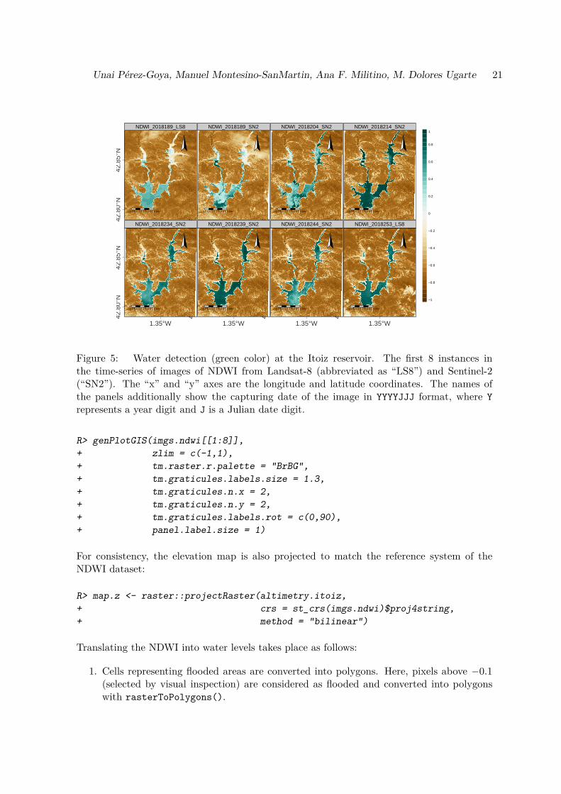
Figure 5: Water detection (green color) at the Itoiz reservoir. The first 8 instances inthe time-series of images of NDWI from Landsat-8 (abbreviated as “LS8”) and Sentinel-2(“SN2”). The “x” and “y” axes are the longitude and latitude coordinates. The names ofthe panels additionally show the capturing date of the image in YYYYJJJ format, where Yrepresents a year digit and J is a Julian date digit.

R> genPlotGIS(imgs.ndwi[[1:8]],+ zlim = c(-1,1),+ tm.raster.r.palette = "BrBG",+ tm.graticules.labels.size = 1.3,+ tm.graticules.n.x = 2,+ tm.graticules.n.y = 2,+ tm.graticules.labels.rot = c(0,90),+ panel.label.size = 1)

For consistency, the elevation map is also projected to match the reference system of theNDWI dataset:

R> map.z <- raster::projectRaster(altimetry.itoiz,+ crs = st_crs(imgs.ndwi)$proj4string,+ method = "bilinear")

Translating the NDWI into water levels takes place as follows:

1. Cells representing flooded areas are converted into polygons. Here, pixels above −0.1(selected by visual inspection) are considered as flooded and converted into polygonswith rasterToPolygons().

22 RGISTools: Time-Series of Remote Sensing Data in R

2. The boundaries of neighboring cells are resolved, and just the edges of the water bodiesremain after st_union(). The output is a ‘MULTIPOLYGON’, which is then coerced intoseparate ‘POLYGON’s by st_cast().

3. The main water body is distinguished from auxiliary reservoirs and isolated missclas-sified pixels by finding the polygon with maximum area. The function st_area()computes the area for each polygon.

4. The elevation map is masked with the line-strings of the shoreline of the main waterbody, which removes every elevation pixel outside the trajectory of the borderline.

5. The median of the shoreline’s elevation gives the estimated water level level.est. Themedian allows to better counteract errors due to the interpolation of the topographicmap and the detection of the shoreline due to the pixel resolution.

R> shorelns <- lapply(as.list(imgs.ndwi),+ function(r){+ water <- raster::rasterToPolygons(clump(r> -0.1),+ dissolve = TRUE)+ shores <- sf::st_union(sf::st_as_sfc(water))+ bodies <- sf::st_cast(shores, "POLYGON")+ areas <- sf::st_area(bodies)+ sf::st_sf(+ sf::st_cast(+ bodies[which(areas == max(areas))],+ "MULTILINESTRING"))})R> shorelns.z <- raster::stack(lapply(shorelns,+ function(x, map.z){+ mask(map.z, x)},+ map.z))R> level.est <- cellStats(shorelns.z, 'median')

To sum up, we build a ‘data.frame’ where the rows represent the sequence of images inthe time-series and the columns represent key aspects of the analysis such as, the satellitemission (sat), the capturing date of the image (date), the observed water levels (obs), andthe estimated water level (est). This ‘data.frame’ summarizes the results of the case study(Figure 6):

R> no.imgs <- nlayers(imgs.ndwi)R> results <- data.frame("sat" = character(no.imgs),+ "date" = structure(integer(no.imgs), class = "Date"),+ "obs" = double(no.imgs),+ "est" = double(no.imgs),+ stringsAsFactors = FALSE)R> results$sat <- ifelse(grepl("LS8", names(imgs.ndwi)), "LS8", "SN2")R> results$date <- genGetDates(names(imgs.ndwi))R> results$obs <- merge(obs.itoiz,results)$level.maslR> results$est <- level.est

Unai Pérez-Goya, Manuel Montesino-SanMartin, Ana F. Militino, M. Dolores Ugarte 23

jul. sep. nov. ene. mar. may.

560

565

570

575

580

Dates

Leve

l (m

.a.s

.l.)

ObsDFLS8SN2

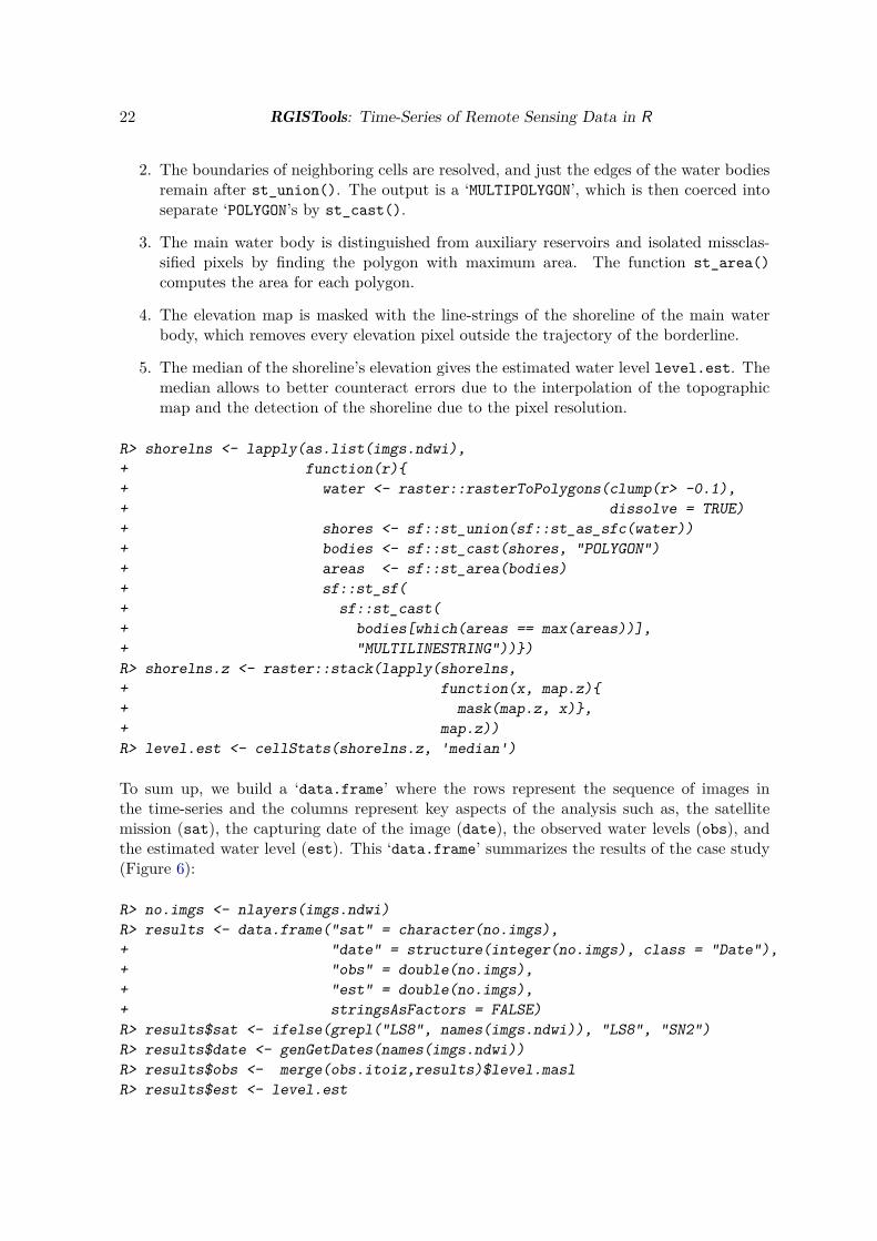
Figure 6: Water levels in the Itoiz reservoir between August 2018 and May 2019. The waterlevels are in meters above sea level (m.a.s.l.). The black line represents the observations.Black and red dots are estimates from Landsat-8 and Sentinel-2 respectively. The dashed linerepresents the combination of Landsat-8 and Sentinel-2 water levels.

Figure 6 shows that the measured water levels are closely followed by the estimates, especiallyby Sentinel-2. Figure 6 also shows how Landsat-8 and Sentinel-2 complement each other togain temporal coverage. We finally compute some metrics of the performance:

R> error <- results$obs - results$estR> mean(abs(error), na.rm = TRUE)

[1] 1.35971

R> mean(abs(error)[results[,"sat"] == "LS8"], na.rm = TRUE)

[1] 2.880557

R> mean(abs(error)[results[,"sat"] == "SN2"], na.rm = TRUE)

[1] 0.8527607

R> cor(results$est, results$obs)

[1] 0.9740032

24 RGISTools: Time-Series of Remote Sensing Data in R

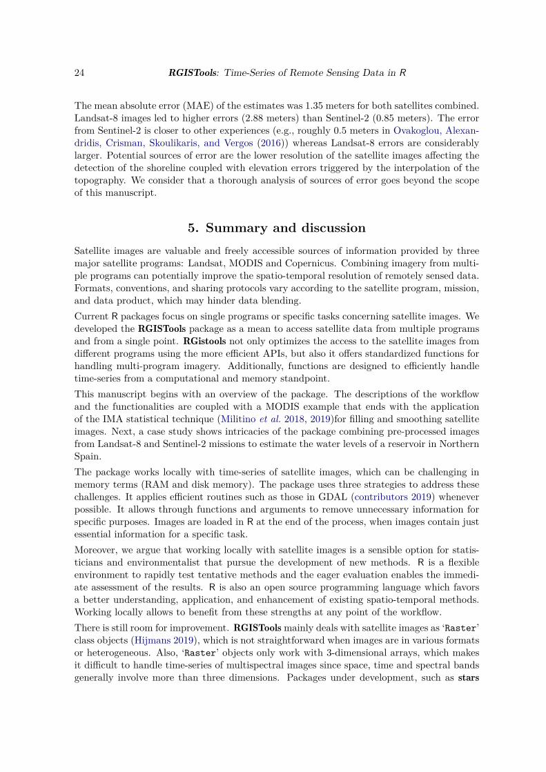
The mean absolute error (MAE) of the estimates was 1.35 meters for both satellites combined.Landsat-8 images led to higher errors (2.88 meters) than Sentinel-2 (0.85 meters). The errorfrom Sentinel-2 is closer to other experiences (e.g., roughly 0.5 meters in Ovakoglou, Alexan-dridis, Crisman, Skoulikaris, and Vergos (2016)) whereas Landsat-8 errors are considerablylarger. Potential sources of error are the lower resolution of the satellite images affecting thedetection of the shoreline coupled with elevation errors triggered by the interpolation of thetopography. We consider that a thorough analysis of sources of error goes beyond the scopeof this manuscript.

5. Summary and discussionSatellite images are valuable and freely accessible sources of information provided by threemajor satellite programs: Landsat, MODIS and Copernicus. Combining imagery from multi-ple programs can potentially improve the spatio-temporal resolution of remotely sensed data.Formats, conventions, and sharing protocols vary according to the satellite program, mission,and data product, which may hinder data blending.Current R packages focus on single programs or specific tasks concerning satellite images. Wedeveloped the RGISTools package as a mean to access satellite data from multiple programsand from a single point. RGistools not only optimizes the access to the satellite images fromdifferent programs using the more efficient APIs, but also it offers standardized functions forhandling multi-program imagery. Additionally, functions are designed to efficiently handletime-series from a computational and memory standpoint.This manuscript begins with an overview of the package. The descriptions of the workflowand the functionalities are coupled with a MODIS example that ends with the applicationof the IMA statistical technique (Militino et al. 2018, 2019)for filling and smoothing satelliteimages. Next, a case study shows intricacies of the package combining pre-processed imagesfrom Landsat-8 and Sentinel-2 missions to estimate the water levels of a reservoir in NorthernSpain.The package works locally with time-series of satellite images, which can be challenging inmemory terms (RAM and disk memory). The package uses three strategies to address thesechallenges. It applies efficient routines such as those in GDAL (contributors 2019) wheneverpossible. It allows through functions and arguments to remove unnecessary information forspecific purposes. Images are loaded in R at the end of the process, when images contain justessential information for a specific task.Moreover, we argue that working locally with satellite images is a sensible option for statis-ticians and environmentalist that pursue the development of new methods. R is a flexibleenvironment to rapidly test tentative methods and the eager evaluation enables the immedi-ate assessment of the results. R is also an open source programming language which favorsa better understanding, application, and enhancement of existing spatio-temporal methods.Working locally allows to benefit from these strengths at any point of the workflow.There is still room for improvement. RGISToolsmainly deals with satellite images as ‘Raster’class objects (Hijmans 2019), which is not straightforward when images are in various formatsor heterogeneous. Also, ‘Raster’ objects only work with 3-dimensional arrays, which makesit difficult to handle time-series of multispectral images since space, time and spectral bandsgenerally involve more than three dimensions. Packages under development, such as stars

Unai Pérez-Goya, Manuel Montesino-SanMartin, Ana F. Militino, M. Dolores Ugarte 25

(Pebesma 2019) and gdalcubes (Appel and Pebesma 2019) are promising solutions. RGIS-GTools already benefits from the computation advantages of stars to compute the remotesensing indices, but its full integration depends on a thoroguh analysis that is still pend-ing. Finally, data fusion techniques frequently involve radar images (Ghamisi, Rasti, Yokoya,Wang, Hofle, Bruzzone, Bovolo, Chi, Anders, Gloaguen et al. 2019). In its current version,the package downloads radar images but does not give support to their processing. These andother challenges that may arise in the future from more complex use cases, will be resolvedin subsequent versions of the package.

Computational detailsThe results in this paper were obtained using R 3.6.2 with the MASS 7.3.51.4 package. Ritself and all packages used are available from the Comprehensive R Archive Network (CRAN)at https://CRAN.R-project.org/.

AcknowledgmentsThis research was supported by the project MTM2017-82553-R (AEI/FEDER, UE). It hasalso received funding from la Caixa Foundation (ID1000010434), Caja Navarra Foundationand UNED Pamplona, under agreement LCF/PR/PR15/51100007.

References

Appel M, Pebesma E (2019). “On-Demand Processing of Data Cubes from Satellite ImageCollections with the gdalcubes Library.” Data, 4(3). doi:10.3390/data4030092. URLhttps://www.mdpi.com/2306-5729/4/3/92.

Azzari G, Jain M, Lobell DB (2017). “Towards Fine Resolution Global Maps of CropYields: Testing Multiple Methods and Satellites in Three Countries.” Remote Sens-ing of Environment, 202, 129–141. doi:10.1016/j.rse.2017.04.014. URL https://doi.org/10.1016/j.rse.2017.04.014.

Belgiu M, Stein A (2019). “Spatiotemporal Image Fusion in Remote Sensing.” Remote sensing,11(7), 818. doi:10.3390/rs11070818. URL https://doi.org/10.3390/rs11070818.

Busetto L, Ranghetti L (2016). “MODIStsp: an R Package for Preprocessing of MODISLand Products Time Series.” Computers & Geosciences, 97, 40–48. doi:10.1016/j.cageo.2016.08.020. URL https://github.com/ropensci/MODIStsp.

contributors G (2019). GDAL/OGR Geospatial Data Abstraction software Library. OpenSource Geospatial Foundation. URL https://gdal.org.

Copernicus (2019). “SciHub Registation.” [Online; accessed 30. Sep. 2019], URL https://scihub.copernicus.eu/dhus/#/self-registration.

Didan K, Munoz AB, Solano R, Huete A (2015). “MODIS Vegetation Index User Guide(MOD13 series).” Vegetation Index and Phenology Lab, The University of Arizona, pp. 1–38.

26 RGISTools: Time-Series of Remote Sensing Data in R

URL https://icdc.cen.uni-hamburg.de/fileadmin/user_upload/icdc_Dokumente/MODIS/MODIS_Collection6_VegetationIndex_UsersGuide_MOD13_V03_June2015.pdf.

dos Santos A (2017). landsat8: Landsat 8 Imagery Rescaled to Reflectance, Radiance and/orTemperature. R package version 0.1-10, URL https://CRAN.R-project.org/package=landsat8.

Du Y, Zhang Y, Ling F, Wang Q, Li W, Li X (2016). “Water Bodies’ Mapping from Sentinel-2 Imagery with Modified Normalized Difference Water Index at 10-m Spatial ResolutionProduced by Sharpening the SWIR Band.” Remote Sensing, 8(4), 354. doi:10.3390/rs8040354. URL https://doi.org/10.3390/rs8040354.

Ebro River Basin Authority (2019). “Automatic Hydrological Information System.” [Online;accessed 1. Oct. 2019], URL http://www.saihebro.com/saihebro/index.php.

EROS ESPA (2019a). “USGS EROS Archive - Landsat Archives - Landsat 8OLI/TIRS Level-2 Data Products - Surface Reflectance.” doi:10.5066/F78S4MZJ.Subset of images from 2018-07-01 to 2019-05-01 intersecting Itoiz., URL https://unavarra-my.sharepoint.com/:u:/g/personal/manuel_montesino_unavarra_es/ERLeCiCl-_dFmN-IwRADZBABAyhfOZqfi2WA6DoUvBWRFQ?e=riILVm.

EROS ESPA (2019b). “USGS EROS Archive - Landsat Archives - Landsat 8OLI/TIRS Level-2 Data Products - Surface Reflectance.” doi:10.5066/F78S4MZJ.Subset of images from 2018-07-01 to 2019-05-01 cropped around Itoiz., URLhttps://unavarra-my.sharepoint.com/:u:/g/personal/manuel_montesino_unavarra_es/EUybRkrcu_dKrh45xlAAsmIB4aN6pGWOBB9J6YhRJBVm-w?e=5MOOIs.

EROS ESPA (2019c). “USGS EROS Archive - Landsat Archives - Landsat 8OLI/TIRS Level-2 Data Products - Surface Reflectance.” doi:10.5066/F78S4MZJ.Cloud masks from 2018-07-01 to 2019-05-01 around Itoiz from the quality band.,URL https://unavarra-my.sharepoint.com/:u:/g/personal/manuel_montesino_unavarra_es/EchN_K1FuWFFmCnL5x0TpX0BJFljFeHpcoiBvWFoTH7Krw?e=RfeoPU.

EROS ESPA (2019d). “USGS EROS Archive - Landsat Archives - Landsat 8OLI/TIRS Level-2 Data Products - Surface Reflectance.” The series of Nor-malized Difference Water Index images from 2018-07-01 to 2019-05-01 cover-ing Itoiz derived from Landsat 8 OLI/TIRS Level-2 Surface Reflectance., URLhttps://unavarra-my.sharepoint.com/:u:/g/personal/manuel_montesino_unavarra_es/EVTOxTv9GtFHtsVf8ch80PsBAGm16HBuEASzsZJbxeecEg?e=U6ZrsP.

ESA (2019a). “Open Access Hub.” [Online; accessed 8. Oct. 2019], URL https://scihub.copernicus.eu.

ESA (2019b). “Sentinel-2 - Missions.” [Online; accessed 8. Oct. 2019], URL https://sentinel.esa.int/web/sentinel/missions/sentinel-2.

ESA (2019c). “Sentinel-2 MSI - Level 2A Product.” Subset of im-ages from 2018-07-01 to 2019-05-01 intersecting Itoiz., URL https://unavarra-my.sharepoint.com/:u:/g/personal/manuel_montesino_unavarra_es/ETn0hSXSi19Fj1S644GS7-UBxX-jx7heB-mxRcN0o7woAg?e=CRXIcx.

Unai Pérez-Goya, Manuel Montesino-SanMartin, Ana F. Militino, M. Dolores Ugarte 27

ESA (2019d). “Sentinel-2 MSI - Level 2A Product.” Subset of images from 2018-07-01to 2019-05-01 cropped around Itoiz., URL https://unavarra-my.sharepoint.com/:u:/g/personal/manuel_montesino_unavarra_es/EXEPbXAzWfxLiHGok73kJoIB0aLhhb71_QDR_B1Jb7jSoA?e=Su4Nxw.

ESA (2019e). “Sentinel-2 MSI - Level 2A Product.” Cloud masks from 2018-07-01 to 2019-05-01 cropped around Itoiz from the quality band., URL https://unavarra-my.sharepoint.com/:u:/g/personal/manuel_montesino_unavarra_es/EXEPbXAzWfxLiHGok73kJoIB0aLhhb71_QDR_B1Jb7jSoA?e=IROOpz.

ESA (2019f). “Sentinel-2 MSI - Level 2A Product.” The series of Normal-ized Difference Water Index images from 2018-07-01 to 2019-05-01 coveringItoiz derived from Sentinel-2 MSI - Level 2A Surface Reflectance., URL https://unavarra-my.sharepoint.com/:u:/g/personal/manuel_montesino_unavarra_es/EbZzHvxB-m1On5MjnVhZp1cB5py3HvLn7Xw5o-gWaZfsdQ?e=YBk2zS.

ESA (2019g). “Sentinel Data Products.” [Online; accessed 30. Sep. 2019], URL https://sentinel.esa.int/web/sentinel/missions/sentinel-2/data-products.

ESA (2019h). “Sentinel Web.” [Online; accessed 8. Oct. 2019], URL https://sentinel.esa.int/web/sentinel/home.

Ghamisi P, Rasti B, Yokoya N, Wang Q, Hofle B, Bruzzone L, Bovolo F, Chi M, AndersK, Gloaguen R, et al. (2019). “Multisource and Multitemporal Data Fusion in RemoteSensing: A Comprehensive Review of the State of the Art.” IEEE Geoscience and RemoteSensing Magazine, 7(1), 6–39. doi:10.1109/MGRS.2018.2890023. URL https://doi.org/10.1109/MGRS.2018.2890023.

Gomez C, Dharumarajan S, Féret JB, Lagacherie P, Ruiz L, Sekhar M (2019). “Use ofSentinel-2 Time-Series Images for Classification and Uncertainty Analysis of Inherent Bio-physical Property: Case of Soil Texture Mapping.” Remote Sensing, 11(5), 565. doi:10.3390/rs11050565. URL https://doi.org/10.3390/rs11050565.

Goslee SC (2011). “Analyzing Remote Sensing Data in R: The landsat Package.” Journal ofStatistical Software, 43(4), 1–25. URL http://www.jstatsoft.org/v43/i04/.

Government of Navarre (2019). “Open Data Navarre - IDENA Download.” [Online; accessed1. Oct. 2019], URL https://idena.navarra.es/Portal/Descargar.

Government of Navarre and Saih (2019). “Auxiliary data.” Topographic map ofItoiz and the measured water levels., URL https://unavarra-my.sharepoint.com/:u:/g/personal/manuel_montesino_unavarra_es/EbdBvgw_fqZMvEnxy-URe_oBJ434rTDRwZOxiMxHeGGK4A?e=Wy8BMZ.

Griffiths P, Nendel C, Hostert P (2019). “Intra-annual Reflectance Composites from Sentinel-2 and Landsat for National-scale Crop and Land Cover Mapping.” Remote Sensing ofEnvironment, 220, 135–151. doi:10.1016/j.rse.2018.10.031. URL https://doi.org/10.1016/j.rse.2018.10.031.

Hijmans RJ (2019). raster: Geographic Data Analysis and Modeling. R package version 2.9-5,URL https://CRAN.R-project.org/package=raster.

28 RGISTools: Time-Series of Remote Sensing Data in R

Hüttich C, Herold M, Wegmann M, Cord A, Strohbach B, Schmullius C, Dech S (2011).“Assessing Effects of Temporal Compositing and Varying Observation Periods for Large-area Land-cover Mapping in Semi-arid Ecosystems: Implications for Global Monitoring.”Remote Sensing of Environment, 115(10), 2445–2459. doi:10.1016/j.rse.2011.05.005.URL https://doi.org/10.1016/j.rse.2011.05.005.

Jean N, Burke M, Xie M, Davis WM, Lobell D, Ermon S (2016). “Combining SatelliteImagery and Machine Learning to Predict Poverty.” Science, 353(6301), 790–794. doi:10.1126/science.aaf7894. URL https://doi.org/10.1126/science.aaf7894.

Jenkerson C (2019). “User Guide: Earth Resources Observation and Science (EROS)Center Science Processing Architecture (ESPA) on Demand Interface.” URLhttps://prd-wret.s3-us-west-2.amazonaws.com/assets/palladium/production/atoms/files/LSDS-1417-ESPA-On-Demand-Interface_User-Guide-v1.pdf.

Ji L, Zhang L, Wylie B (2009). “Analysis of Dynamic Thresholds for the Normalized DifferenceWater Index.” Photogrammetric Engineering & Remote Sensing, 75(11), 1307–1317. doi:10.14358/PERS.75.11.1307. URL https://doi.org/10.14358/PERS.75.11.1307.

Mattiuzzi M, Detsch F (2019). MODIS: Acquisition and Processing of MODIS Products. Rpackage version 1.1.5, URL https://CRAN.R-project.org/package=MODIS.

Matzke NJ (2013). modiscloud: An R Package for Processing MODIS Level 2 Cloud MaskProducts. This code was developed for the following paper: Goldsmith, Gregory; Matzke,Nicholas J.; Dawson, Todd (2013). The incidence and implications of clouds for cloudforest plant water relations. Ecology Letters, 16(3), 307-314. doi: 10.1111/ele.12039, URLhttp://cran.r-project.org/web/packages/modiscloud/index.html.

McFeeters SK (1996). “The Use of the Normalized Difference Water Index (NDWI) inthe Delineation of Open Water Features.” International Journal of Remote Sensing,17(7), 1425–1432. doi:10.1080/01431169608948714. URL https://doi.org/10.1080/01431169608948714.

Militino AF, Ugarte MD, Pérez-Goya U (2018). “Improving the Quality of Satellite ImageryBased on Ground-Truth Data from Rain Gauge Stations.” Remote Sensing, 10(3), 398.doi:10.3390/rs10030398. URL https://doi.org/10.3390/rs10030398.

Militino AF, Ugarte MD, Pérez-Goya U, Genton MG (2019). “Interpolation of the MeanAnomalies for Cloud Filling in Land Surface Temperature and Normalized Difference Veg-etation Index.” IEEE Transactions on Geoscience and Remote Sensing, 57(8), 6068–6078. doi:10.1109/TGRS.2019.2904193. URL https://doi.org/10.1109/TGRS.2019.2904193.

NASA (2019a). “Earthdata.” [Online; accessed 8. Oct. 2019], URL https://earthdata.nasa.gov.

NASA (2019b). “EarthData Registration.” [Online; accessed 30. Sep. 2019], URL https://urs.earthdata.nasa.gov/users/new.

NASA (2019c). “LP DAAC Services Documentation.” [Online; accessed 8. Oct. 2019], URLhttps://lpdaacsvc.cr.usgs.gov/services.

Unai Pérez-Goya, Manuel Montesino-SanMartin, Ana F. Militino, M. Dolores Ugarte 29

NASA (2019d). “MODIS Data Products.” [Online; accessed 30. Sep. 2019], URL https://modis.gsfc.nasa.gov/data/dataprod/.

NASA (2019e). “MODIS Web.” [Online; accessed 8. Oct. 2019], URL https://modis.gsfc.nasa.gov/.

Nauss T, Meyer H, Detsch F, Appelhans T (2015). “Manipulating Satellite Data with satel-lite.” unpublished, na(na), na–na. URL www.environmentalinformatics-marburg.de.

Nychka D, Furrer R, Paige J, Sain S (2017). “fields: Tools for Spatial Data.” doi:10.5065/D6W957CT. R package version 9.8-3, URL https://github.com/NCAR/Fields.

ORNL DAAC (2019). “MODIS/VIIRS Documentation.” [Online; accessed 8. Oct. 2019],URL https://modis.ornl.gov/documentation.

Ovakoglou G, Alexandridis TK, Crisman TL, Skoulikaris C, Vergos GS (2016). “Use ofMODIS Satellite Images for Detailed Lake Morphometry: Application to Basins with LargeWater Level Fluctuations.” International Journal of Applied Earth Observation and Geoin-formation, 51, 37–46. doi:10.1016/j.jag.2016.04.007. URL https://doi.org/10.1016/j.jag.2016.04.007.

Paul F, Winsvold S, Kääb A, Nagler T, Schwaizer G (2016). “Glacier Remote Sens-ing Using Sentinel-2. Part II: Mapping Glacier Extents and Surface Facies, and Com-parison to Landsat 8.” Remote Sensing, 8(7), 575. doi:10.3390/rs8070575. URLhttps://doi.org/10.3390/rs8070575.

Pebesma E (2004). “Multivariable Geostatistics in S: the gstat Package.” Computers &Geosciences, 30, 683–691. doi:10.1016/j.cageo.2004.03.012. URL https://doi.org/10.1016/j.cageo.2004.03.012.

Pebesma E (2018). “Simple Features for R: Standardized Support for Spatial Vector Data.”The R Journal, 10(1), 439–446. doi:10.32614/RJ-2018-009. URL https://doi.org/10.32614/RJ-2018-009.

Pebesma E (2019). stars: Spatiotemporal Arrays, Raster and Vector Data Cubes. R packageversion 0.4-0, URL https://CRAN.R-project.org/package=stars.

Pérez-Goya U, Militino AF, Ugarte MD, Montesino-SanMartin M (2019). RGISTools:Handling Multiplatform Satellite Images. R package version 0.9.7, URL https://CRAN.R-project.org/package=RGISTools.

R Core Team (2019). R: A Language and Environment for Statistical Computing. R Founda-tion for Statistical Computing, Vienna, Austria. URL https://www.R-project.org/.

Ranghetti L, Busetto L (2019). sen2r: Find, Download and Process Sentinel-2 Data. doi:10.5281/zenodo.1240384. R package version 1.2.1, URL http://sen2r.ranghetti.info.

Riyas MJ, Syed TH (2018). ASIP: Automated Satellite Image Processing. R package version0.4.9, URL https://CRAN.R-project.org/package=ASIP.

Rouse Jr JW (1972). “Monitoring the Vernal Advancement and Retrogradation (Green WaveEffect) of Natural Vegetation.” URL https://ntrs.nasa.gov/archive/nasa/casi.ntrs.nasa.gov/19730009607.pdf.

30 RGISTools: Time-Series of Remote Sensing Data in R

Santacruz A, Developers SA (2017). SkyWatchr: Search and Download Satellite ImageryUsing the SkyWatch API. R package version 0.8-2, URL https://CRAN.R-project.org/package=SkyWatchr.

Shen H, Li X, Cheng Q, Zeng C, Yang G, Li H, Zhang L (2015). “Missing InformationReconstruction of Remote Sensing Data: A Technical Review.” IEEE Geoscience andRemote Sensing Magazine, 3(3), 61–85. doi:10.1109/MGRS.2015.2441912. URL https://doi.org/10.1109/MGRS.2015.2441912.

Signer J, Trubilowicz J (2016). MODISSnow: Provides a Function to Download MODISSnow Cover. R package version 0.1.0.0, URL https://CRAN.R-project.org/package=MODISSnow.

Swinbourne MJ, Taggart DA, Swinbourne AM, Lewis M, Ostendorf B (2018). “Using SatelliteImagery to Assess the Distribution and Abundance of Southern Hairy-nosed Wombats(Lasiorhinus latifrons).” Remote Sensing of Environment, 211, 196–203. doi:10.1016/j.rse.2018.04.017. URL https://doi.org/10.1016/j.rse.2018.04.017.

Tennekes M (2018). “tmap: Thematic Maps in R.” Journal of Statistical Software, 84(6),1–39. doi:10.18637/jss.v084.i06. URL https://doi.org/10.18637/jss.v084.i06.

Tuck SL, Phillips HR, Hintzen RE, Scharlemann JP, Purvis A, Hudson LN (2014). “MODIS-Tools – Downloading and Processing MODIS Remotely Sensed Data in R.” Ecology andEvolution, 4(24), 4658–4668. doi:10.1002/ece3.1273. URL http://onlinelibrary.wiley.com/doi/10.1002/ece3.1273/full.

USGS (2019a). “Landsat Shapefiles and KML Files.” [Online; accessed8. Oct. 2019], URL https://www.usgs.gov/land-resources/nli/landsat/landsat-shapefiles-and-kml-files.

USGS (2019b). “Landsat Web.” [Online; accessed 8. Oct. 2019], URL https://www.usgs.gov/land-resources/nli/landsat.

Vermonte E (2019a). “MODIS/Terra Surface Reflectance Daily L2G Global 1 km and500 m 250m SIN Grid V006 [Data set], NASA EOSDIS LP DAAC.” doi:10.5067/MODIS/MOD09GA.006. Subset of MOD09GA dataset, between 2018-08-02 and 2018-08-09., URL https://unavarra-my.sharepoint.com/:u:/g/personal/manuel_montesino_unavarra_es/Ee-r9wnYkpRMiUYSE4tTZkYBwktsMZ7rkzH_SJPMhlsbJw?e=IIeQW.

Vermonte E (2019b). “MODIS/Terra Surface Reflectance Daily L2G Global 1 kmand 500 m 250m SIN Grid V006 [Data set], NASA EOSDIS LP DAAC.” doi:10.5067/MODIS/MOD09GA.006. Subset of MOD09GA dataset, between 2018-08-02 and2018-08-09 and cropped over Navarre., URL https://unavarra-my.sharepoint.com/:u:/g/personal/manuel_montesino_unavarra_es/EYoHAOFS6uJDpW4u0rL7_n8BLOQ23lKgtAHMNfZ9Pvpfqw?e=wtlkBN.

Vermote E (2015). “MODIS Surface Reflectance User’s Guide.” URL https://landweb.modaps.eosdis.nasa.gov/QA_WWW/forPage/user_guide/MOD09_UserGuide_v1.4.pdf.

Zhu Z, Qiu S, He B, Deng C (2018). “Cloud and Cloud Shadow Detection for LandsatImages: The Fundamental Basis for Analyzing Landsat Time Series.” In Remote SensingTime Series Image Processing, pp. 25–46. CRC Press.

Unai Pérez-Goya, Manuel Montesino-SanMartin, Ana F. Militino, M. Dolores Ugarte 31

Affiliation:Unai Pérez-GoyaDepartment of Statistics, Computer Science, and MathematicsPublic University of Navarre31006 Pamplona, SpainE-mail: unai.perez@unavarra.esURL: https://www.unavarra.es/pdi?uid=811058

Manuel Montesino-SanMartinDepartment of Statistics, Computer Science, and MathematicsPublic University of Navarre31006 Pamplona, SpainE-mail: manuel.montesino@unavarra.es

Ana F. MilitinoDepartment of Statistics, Computer Science, and MathematicsPublic University of Navarre31006 Pamplona, SpainE-mail: militino@unavarra.esURL: https://www.unavarra.es/personal/amilitino

Maria Dolores UgarteDepartment of Statistics, Computer Science, and MathematicsPublic University of Navarre31006 Pamplona, SpainE-mail: lola@unavarra.esURL: https://www.unavarra.es/personal/lugarte