Embed Size (px)
Citation preview

PhD thesis
LHC Interaction regionupgrade
Riccardo de Maria
2008

2
Abstract
The thesis analyzes the interaction region of the Large Hadron Collider(LHC). It proposes, studies and compares several upgrade options. Theinteraction region is the part of the LHC that hosts the particle detectorswhich analyze the collisions. An upgrade of the interaction region can po-tentially increase the number of collision events and therefore it is possibleto accumulate and study a larger set of experimental data.
The main object of study are the focus systems that consist of a set ofmagnets in charge of concentrating the particle beams in a small spot at theinteraction points.
The thesis uses the methods of beam optics and beam dynamics to designnew interaction regions. Two design schemes are compared with a detailedanalysis of the performance of several implementations. The design of thelayouts takes into account the technical limitations that will affect possiblerealizations.
Either analytical or numerical methods are used to evaluate the perfor-mance of the proposed layouts. The thesis presents new general methodsthat can be used for problems beyond the scope of the thesis. An analyticalmethod has been developed for finding the intrinsic limitations of the focussystems. It allows to perform an exhaustive scan of the accessible parameterspace and thus presents an efficient tool for guiding the design process. Anumerical optimization routine and several enhancements have been imple-mented in MADX, a code for beam optics design. The routines simplify thesolution of several optimization problems of beam optics.
Keywords: accelerators design, beam optics, beam dynamics.
3

4

Abstract
Con questa tesi si è voluto approfondire lo studio della zona di interazionedel Large Hadron Collider (LHC) allo scopo di proporre possibili soluzionidi sviluppo (upgrade) della macchina.
La zona di interazione è quella parte di LHC che contiene i rivelatori diparticelle che analizzano le collisioni. Un upgrade della zona di interazionepermetterebbe potenzialmente di aumentare il numero di eventi rilevabilinella singola collisione e quindi di accumulare e studiare una quantità piùelevata di dati sperimentali.
L’oggetto principale dello studio sono i sistemi focalizzanti per le particelleche consistono in una serie di magneti capaci di concentrare i fasci convergentiin una piccola regione nel punto di interazione.
Questa tesi usa metodi della ottica e della dinamica dei fasci per proget-tare nuove zone di interazione. Sono stati confrontati due schemi tecnologicialternativi, ponendo particolare attenzione alle differenti limitazioni tecnicheche possono diventare pregiudicanti al momento della realizzazione.
Per determinare le performance degli schemi proposti sono usati metodianalitici e numerici. La tesi presenta inoltre metodi generali applicabili inconstesti diversi.
In particolare è stato sviluppato un metodo analitico per l’individuazionedelle limitazioni intrinseche dei sistemi focalizzanti per particelle. Il meto-do permette di effettuare una analisi completa dello spazio dei parametriaccessibile e fornisce un efficiente strumento per la progettazione.
Un metodo numerico di ottimizzazione e diversi miglioramenti sono statiideati e implementati al fine di potenziare il codice MADX per la progettazio-ne degli acceleratori. Le modifiche introdotte rendono più facile la soluzionedi diversi problemi di ottimizzazione dell’ottica dei fasci.
Parole chiavi: progetto di acceleratori, ottica dei fasci di particelle, dina-mica dei fasci di particelle.

6

Contents
1 Introduction 111.1 Synopsis . . . . . . . . . . . . . . . . . . . . . . . . . . . . . . 111.2 Contributions associated with this thesis . . . . . . . . . . . . 121.3 Acknowledgment . . . . . . . . . . . . . . . . . . . . . . . . . 12
2 The LHC Upgrade 132.1 Introduction . . . . . . . . . . . . . . . . . . . . . . . . . . . . 132.2 The Large Hadron Collider . . . . . . . . . . . . . . . . . . . . 13
2.2.1 Top energy . . . . . . . . . . . . . . . . . . . . . . . . 152.2.2 Luminosity . . . . . . . . . . . . . . . . . . . . . . . . 15
2.3 Peak luminosity . . . . . . . . . . . . . . . . . . . . . . . . . . 162.3.1 Bunch intensity . . . . . . . . . . . . . . . . . . . . . . 172.3.2 Number of bunches . . . . . . . . . . . . . . . . . . . . 182.3.3 Transverse beam size at the IP . . . . . . . . . . . . . 192.3.4 Geometric reduction factor . . . . . . . . . . . . . . . . 19
2.4 Conclusion . . . . . . . . . . . . . . . . . . . . . . . . . . . . . 22
3 LHC interaction region layout 253.1 Introduction . . . . . . . . . . . . . . . . . . . . . . . . . . . . 253.2 Beam dynamics . . . . . . . . . . . . . . . . . . . . . . . . . . 25
3.2.1 Transverse dynamics . . . . . . . . . . . . . . . . . . . 273.2.2 Linear dynamics . . . . . . . . . . . . . . . . . . . . . 283.2.3 Non linear perturbations . . . . . . . . . . . . . . . . . 313.2.4 Dispersion and chromatic effects . . . . . . . . . . . . . 32
3.3 Interaction region layout . . . . . . . . . . . . . . . . . . . . . 353.3.1 Detector area . . . . . . . . . . . . . . . . . . . . . . . 353.3.2 TAS . . . . . . . . . . . . . . . . . . . . . . . . . . . . 363.3.3 IR Triplets . . . . . . . . . . . . . . . . . . . . . . . . . 363.3.4 Separation/recombination section . . . . . . . . . . . . 403.3.5 Matching section . . . . . . . . . . . . . . . . . . . . . 423.3.6 Dispersion suppressor . . . . . . . . . . . . . . . . . . . 43
7

Contents
3.4 Limitations of the nominal interaction region layout . . . . . . 443.4.1 Aperture . . . . . . . . . . . . . . . . . . . . . . . . . . 443.4.2 Field quality and long term stability . . . . . . . . . . 453.4.3 Beam beam interactions and geometric reduction factor 463.4.4 Heat deposition . . . . . . . . . . . . . . . . . . . . . . 483.4.5 Radiation damage . . . . . . . . . . . . . . . . . . . . . 483.4.6 Chromatic aberrations . . . . . . . . . . . . . . . . . . 483.4.7 Matchability . . . . . . . . . . . . . . . . . . . . . . . . 48
3.5 Conclusion . . . . . . . . . . . . . . . . . . . . . . . . . . . . . 49
4 Dipole first layout 514.1 Introduction . . . . . . . . . . . . . . . . . . . . . . . . . . . . 514.2 Motivations . . . . . . . . . . . . . . . . . . . . . . . . . . . . 514.3 Dipole first layout . . . . . . . . . . . . . . . . . . . . . . . . . 524.4 Collision optics . . . . . . . . . . . . . . . . . . . . . . . . . . 534.5 Crossing scheme . . . . . . . . . . . . . . . . . . . . . . . . . . 554.6 Mechanical aperture . . . . . . . . . . . . . . . . . . . . . . . 574.7 Chromaticity . . . . . . . . . . . . . . . . . . . . . . . . . . . 594.8 Dynamic aperture . . . . . . . . . . . . . . . . . . . . . . . . . 60
4.8.1 DA from measured errors . . . . . . . . . . . . . . . . 624.8.2 Multipole by multipole analysis . . . . . . . . . . . . . 62
4.9 Squeeze . . . . . . . . . . . . . . . . . . . . . . . . . . . . . . 674.10 Conclusion . . . . . . . . . . . . . . . . . . . . . . . . . . . . . 67
5 Quadrupole first layouts 695.1 Introduction . . . . . . . . . . . . . . . . . . . . . . . . . . . . 695.2 Motivation . . . . . . . . . . . . . . . . . . . . . . . . . . . . . 695.3 Optimization of triplet layout . . . . . . . . . . . . . . . . . . 69
5.3.1 Final focus design . . . . . . . . . . . . . . . . . . . . . 715.3.2 Parameters . . . . . . . . . . . . . . . . . . . . . . . . 735.3.3 Approximation of the equations . . . . . . . . . . . . . 735.3.4 Normalization . . . . . . . . . . . . . . . . . . . . . . . 755.3.5 Scalings . . . . . . . . . . . . . . . . . . . . . . . . . . 755.3.6 Parameter space . . . . . . . . . . . . . . . . . . . . . 78
5.4 Four flavors of quadrupole first layouts . . . . . . . . . . . . . 805.5 Crossing scheme . . . . . . . . . . . . . . . . . . . . . . . . . . 855.6 Mechanical aperture . . . . . . . . . . . . . . . . . . . . . . . 865.7 Chromaticity . . . . . . . . . . . . . . . . . . . . . . . . . . . 885.8 Dynamic aperture . . . . . . . . . . . . . . . . . . . . . . . . . 885.9 Transition to injection . . . . . . . . . . . . . . . . . . . . . . 915.10 Conclusion . . . . . . . . . . . . . . . . . . . . . . . . . . . . . 91
8

Contents
6 Conclusions 93
A Optimization tools for accelerator optics 95A.1 Introduction . . . . . . . . . . . . . . . . . . . . . . . . . . . . 95A.2 Optimization and least-sqaure fitting . . . . . . . . . . . . . . 96A.3 Singular value decomposition . . . . . . . . . . . . . . . . . . 97A.4 JACOBIAN algorithm . . . . . . . . . . . . . . . . . . . . . . 98A.5 Conclusion . . . . . . . . . . . . . . . . . . . . . . . . . . . . . 101
9

Contents
10

Chapter 1
Introduction
1.1 Synopsis
The topic of the thesis concerns the upgrade of the Large Hadron Colliderinteraction region.
Chapter 2 presents an introduction of the LHC performance, limitationsand upgrade strategies. The chapter concludes by identifying the upgrade ofthe interaction regions as a viable option for increasing the luminosity in theLHC by reducing the beam size at the interaction points.
Chapter 3 shows the basic tools of beam transverse dynamics, analyzesthe present LHC high luminosity interaction region, identifies the limitationsarising from a reduction of the beam size at the interaction points and con-cludes by presenting an upgrade target and two alternative options (dipolefirst and quadrupole first) which try to overcome different limitations.
Chapter 4 focuses on a realistic design of a dipole first upgrade layoutwith an analysis of the merits and challenges.
Chapter 5 focuses on realistic designs for quadrupole first layouts with ananalysis of the merits and challenges. The chapter shows an original methodfor identifying the theoretical limitations of the quadrupole first designs andfinding optimized layouts.
Chapter 6 concludes the thesis by summing up the results, comparingthe presented options and introducing future plans of CERN concerning theLHC upgrade.
The appendix presents a numerical optimization algorithm implementedin an existing program for accelerator design (MADX).
11
Introduction 1.3
1.2 Contributions associated with this thesisThe original work incorporated in and arising from this thesis can be orga-nized in the following categories:
1. Original design of a dipole first option with analysis of hardware re-quirements, performance, limitations and correction strategies for aber-rations ( [dM05], [dMBR06], [dM07b], [FGdMG07]).
2. Orginal designs of low gradient quadrupoles first options with analy-sis of hardware requirements, performance, limitations. Proposal forPhase I upgrade ( [dMB06], [BdM07], [BdMO07] ).
3. Optics design of high gradient quadrupole first options ( [KAM+07] ).
4. Development of analytical tools for final focus design ( [dM07a] ).
5. Optimization tools for optics design software and automated proce-dures for generating optics transitions ( [dMSS06], [SSdMF06]).
1.3 AcknowledgmentThanks for the continuous support and inspiration to: Aurelio Bay, OliverBrüning, Ulrich Dorda, Simone Gilardoni, Massimo Giovannozzi, StéphaneFartoukh, Tom Kroyer, Frank Schmidt, Rogelio Tomas, Thys Risselada,Leonid Rivkin, Albin Wrulich.
Many thanks for the helpful discussions and ideas to: Erik Adli, ElenaBenedetto, Sandro Bonacini, Chiara Bracco, Roderik Bruce, Helmut Burkhardt,Rama Calaga, Werner Herr, Jean Pierre Kouchuck, Ramesh Gubta, Eti-enne Forest, Andrea Franchi, Jean Bernard Jeanneret, John Johnstone, JohnJowet, Emanuale Laface, Andrea Latina, Peter Limon, Daniela Macina,Nicola Mokhov, Yannis Papaphilippou, Steve Peggs, Diego Quatraro, Ste-fano Redaelli, Giovanni Rumolo, Guillome Robert-Demolaize, Federico Ron-carolo, Benoit Salvant, Tanaji Sen, Vladimir Shiltsev, Guido Sterbini, WalterScandale, Ezio Todesco, Frank Zimmermann.
I acknowledge the support of the European Community-Research Infras-tructure Activity under the FP6 "Structuring the European Research Area"programme (CARE, contract number RII3-CT-2003-506395).
12

Chapter 2
The LHC Upgrade
2.1 IntroductionIn this chapter I will examine the key parameter estimates for the LargeHadron Collider (LHC). An analysis of the limiting factors in the LHC per-formance will lead to an overview of future upgrade strategies. In the finalpart I will list the pros and cons of the interaction region upgrade.
2.2 The Large Hadron ColliderThe scope of the LHC is to find experimental evidence of the Higgs mech-anism which generate particle masses, gluon plasma, to perform precisionmeasurements for validating the standard model theory and to explore newphysics frontiers ([Gia99]).
The LHC is designed to fulfill this goal by colliding hadrons at unprece-dented energies (14 TeV in the center of mass in proton-proton collisionsand 5.52 TeV for nucleons in lead ions), and a very high luminosity (around1034 cm−2 s−1) which leads to around 40 proton-proton collisions in two ex-periments every 25 ns. Hadrons assure a large spectrum of events productionbecause the energy of nucleons is shared between the elementary constituents(quarks and gluons).
The LHC is a synchroton that consists of a 26.7 km ring where twocounter-rotating beams collide in four interaction points (IP). The beams cir-culate in separate magnetic channels (they require opposite magnetic field)and are recombined before the IP. At the IP there is an experimental areaequipped with particle detectors which are able to reconstruct the eventsoccurred by tracking the fragments of the collisions (see Fig. 2.2.1). For anintroduction on the machine see [BC07] and [BCL+04]. .
13

The LHC Upgrade 2.2
Figure 2.2.1 LHC schematic. LHC is composed of 8 arcs and 8 long straightsections (LSS). Two counter-rotating beams cross and collide in 4 interactionregion (IR1,IR2,IR5,IR8). The other straight sections, called interaction re-gions (IR), are for beam collimation (IR3,IR7), RF beam acceleration (IR4)and beam dump (IR6).
14

The LHC Upgrade 2.2
In 2001 CERN launched an R&D program (see [Zim08]) to study thefeasibility of an upgrade of the two key parameters, energy and luminosity(see [GMV02], [BCG+02]).
An increase of the particle energy can mainly be useful for extendingthe physics reach of the LHC, while an increase of the luminosity will helpexperiments to collect more data which translate into more accurate mea-surements or more chances to study rare events (like the detection of Higgsbosons decays).
An analysis of these two key parameters will identify possible upgradescenarios.
2.2.1 Top energyThe maximum energy achievable by the particles in the LHC (E ' pc =7 TeV) is limited by the radius of tunnel arcs (ρ = 3.5 km) and/or by themaximum bending field generated by the dipole magnets (B = 8.33 T). Thesequantities are in fact related by the equation:
p
e= fbendBρ (2.2.1)
where fbend is a factor smaller than 1 (0.8 for the LHC resulting in a maxi-mum bending radius of 2.8 km) which takes into account the fact that the arcscannot be completely filled by bending magnets since space must be reservedfor experimental areas, stabilizing magnets, accelerating radio-frequency cav-ities, collimators and diagnostic components.
An increase of the energy can only be achieved by building a larger ringor by improving the magnet technology and replacing the existing magnetswith new magnets that feature an increased bending field. Both of theseoptions require enormous costs and will not be treated in this thesis.
2.2.2 LuminosityThe collision rate is determined by the accelerator luminosity which is afigure of merit defined by the beam parameters and accelerator lattice. Itrelates the cross section of an event to the event rate via the formula:
dRdt = Lσ [L] = cm−2 s−1 (2.2.2)
where R is the number of events and σ is the cross section of the event. Forcalculating the overall proton collision rate, the total inelastic cross section
15

The LHC Upgrade 2.3
for protons is estimated to be around 100 mb (a barn , b, correspond to1 · 10−24 cm2) and the luminosity ranges between 1 · 1034 cm−2 s−1 (nominalperformance) and 2.3 · 1034 cm−2 s−1 (ultimate performance).
As the LHC is a cycled machine, the luminosity is not constant overtime. The particles must first be injected in the LHC with a momentumof 450G eV/c by the injector chain of accelerators (Source, Linac2, Booster,PS, SPS), then slowly accelerated (for about half an hour) and finally put incollision when they reach 7 TeV. At this time the luminosity will be at itspeak and collision rate will be maximum. After the first collisions the beamparameters change and the luminosity decays. The processes responsible forthe decay are the collisions themselves (resulting in a lifetime of 45 hours) andbeam blow-up due intra-beam scattering, rest gas collision, noise, magneticfield imperfections, long range beam beam interaction (all of them slightlycompensated by the synchrotron radiation damping). The net luminositylifetime, including all of these effects reduces to about 15 hours ([BCL+04]).When the luminosity is too low, a fresh beam is injected in order to maximizethe integrated luminosity.
The integrated luminosity in fact has more physical relevance than thepeak luminosity because it gives a measure of the amount of data acquired bythe experiments over time. On the other hand it is more difficult to estimatedue to the uncertainty involved in several processes. A discussion on theoptimization of the integrated luminosity is left out from the thesis whilea discussion on the peak luminosity, which can easily be estimated by thebeam parameters, will be the topic of the next section.
2.3 Peak luminosityThe peak luminosity can be estimated (see [HM03]) from the beam parame-ters using:
L = N2b fnb
4πσ∗xσ∗yF (θc, σx, σz), (2.3.1)
where f is the beam revolution frequency, Nb the number of protons perbunch or bunch intensity, nb the number of bunches, σ∗x, σ∗y are the transverseRMS beam sizes at the IP, F the geometric loss factor which depends onother beam parameters (beam crossing angle θc , longitudinal beam size σzand transverse beam size in the crossing plane).
This formula is valid for two Gaussian beams of equal size and if thehourglass effect is negligible (see [HM03]). The hourglass effect, which in our
16
The LHC Upgrade 2.3
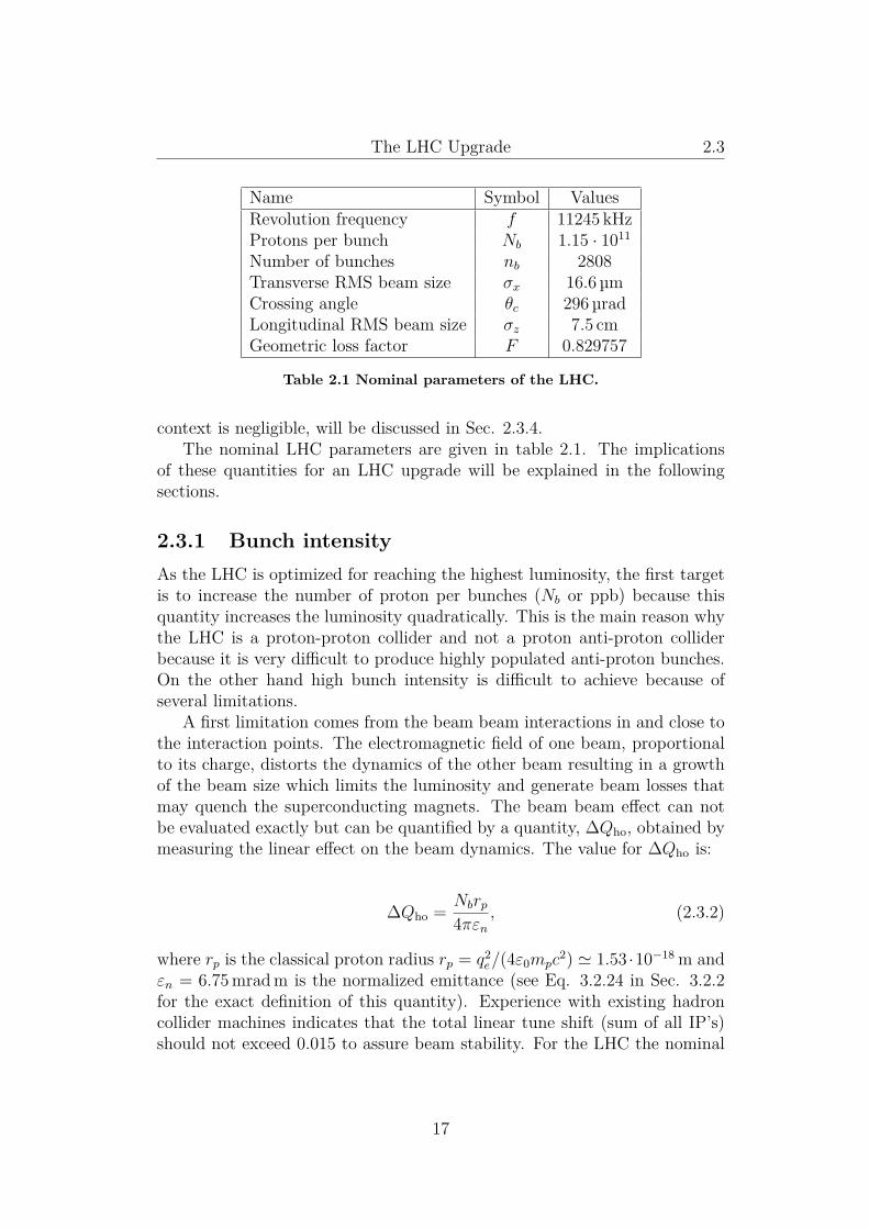
Name Symbol ValuesRevolution frequency f 11245 kHzProtons per bunch Nb 1.15 · 1011
Number of bunches nb 2808Transverse RMS beam size σx 16.6 µmCrossing angle θc 296 µradLongitudinal RMS beam size σz 7.5 cmGeometric loss factor F 0.829757
Table 2.1 Nominal parameters of the LHC.
context is negligible, will be discussed in Sec. 2.3.4.The nominal LHC parameters are given in table 2.1. The implications
of these quantities for an LHC upgrade will be explained in the followingsections.
2.3.1 Bunch intensityAs the LHC is optimized for reaching the highest luminosity, the first targetis to increase the number of proton per bunches (Nb or ppb) because thisquantity increases the luminosity quadratically. This is the main reason whythe LHC is a proton-proton collider and not a proton anti-proton colliderbecause it is very difficult to produce highly populated anti-proton bunches.On the other hand high bunch intensity is difficult to achieve because ofseveral limitations.
A first limitation comes from the beam beam interactions in and close tothe interaction points. The electromagnetic field of one beam, proportionalto its charge, distorts the dynamics of the other beam resulting in a growthof the beam size which limits the luminosity and generate beam losses thatmay quench the superconducting magnets. The beam beam effect can notbe evaluated exactly but can be quantified by a quantity, ∆Qho, obtained bymeasuring the linear effect on the beam dynamics. The value for ∆Qho is:
∆Qho = Nbrp4πεn
, (2.3.2)
where rp is the classical proton radius rp = q2e/(4ε0mpc
2) ' 1.53 ·10−18 m andεn = 6.75 mrad m is the normalized emittance (see Eq. 3.2.24 in Sec. 3.2.2for the exact definition of this quantity). Experience with existing hadroncollider machines indicates that the total linear tune shift (sum of all IP’s)should not exceed 0.015 to assure beam stability. For the LHC the nominal
17

The LHC Upgrade 2.3
intensity Nb = 1 · 1011 yields ∆Qho = 0.0032 per IP, while the ultimateintensity is defined for Nb = 2.3 · 1011 which is at the limit for the beambeam tune shift.
The beams continue to interact nearby the interaction region for the rea-son discussed in Sec. 2.3.4 and 3.4.3. This type of interactions are called longrange beam beam interactions (LRBB interactions). The LRBB interactionspresent similar limitations to the head-on beam beam interaction and theireffects depend again on the bunch intensity (see [CT99]).
The bunch intensity enters in the definition of the beam current which isresponsible to another set of limitations that will be discussed in Sec. 2.3.2.
The effects mentioned above show that boosting the luminosity by anincrease of the bunch intensity is a delicate issue because it affects a largenumber of machine subsystems. As an upgrade project, the increase of thebunch intensity has a large potential but also a large uncertainty.
2.3.2 Number of bunchesThe bunch intensity, together with the number of bunches nb, define thevalue of the beam current:
Ib = Nbnbfq. (2.3.3)
The number of bunches depends on the bunch spacing and filling factor.It affects the multi-bunch instabilities, the heat load in the cryogenic system,the beam stored energy (350 MJ at a particle energy of 7 TeV and nominalintensity) and, in addition, the number of long range beam beam interactions.
The multi-bunch instabilities arise from the electromagnetic wake fieldsin the beam pipe interacting with beam (see [Cha93]).
As the bunch pass through the beam pipe, it creates also image currentswhich are proportional to the beam current. They deposite heat close thesuperconductors triggering a quench if the cryogenic system does not removethe heat.
In addition, the bunch charge stimulates electron emission and the buildup of an electron cloud. This in turn genetates additional heat and causesbeam instabilities.
As the LHC is a superconducting machine, all the heat must be extractedat cryogenic temperatures (1.8 K) by the cryogenic system which is alreadyat limits of its heat transfer capabilities or cooling power.
On top of this the stored beam energy is proportional to the bunch cur-rent. A large stored beam energy creates hazard to the equipments andrequire sophisticated protection mechanisms.
18

The LHC Upgrade 2.3
A decrease of the bunch spacing, which would be required to increase thenumber of bunches, will increase the number of the long range beam beaminteraction as it will be discussed in Sec. 2.3.4.
In conclusion, an increase of the number of bunches show similar draw-backs of an increase of the bunch intensity but the increase of luminosity isonly linear.
2.3.3 Transverse beam size at the IPIf we neglect the geometric reduction factor, the inverse of the transversebeam size (or beam cross section) at the IP gives a linear increase of the lu-minosity. It is a local quantity that affects a limited part of the accelerator,if we exclude the aberrations of the beam that tend to increase as the beamsize diminishes. These facts make it a good candidate for an upgrade projectbecause a limited intervention is able to boost the performance without af-fecting the rest of the machine. The upgrade of the interaction region is themain topic of this thesis.
The beam size at the IP is determined by the focusing properties ofthe quadrupole magnets and the layout of the long straight section (LSS)which connects the ring arcs and hosts the experiments. The fact that thequadrupole strength of the magnets and the total length of the LSS arelimited, poses a limit on the minimum beam size achievable in the LHC.In addition, another limits comes from the geometric reduction factor whichstarts to play a role in the luminosity estimation when the transverse beamsize is small compared to the longitudinal one, as we will see in Sec. 2.3.4.
2.3.4 Geometric reduction factorThe geometric reduction factor enters in the luminosity estimation (Eq.2.3.1) when the beams collide with a crossing angle. When the bunchescollide with a crossing angle the effective area of interaction is reduced andthe luminosity as well (see fig 2.3.2) .
The geometric reduction factor can be computed using:
F = 1√√√√1 +(θcσz2σ∗x
)2, (2.3.4)
where θc is the crossing angle, σz is the longitudinal beam size, σ∗x is thetransverse beam size in the crossing plane.
19

The LHC Upgrade 2.3
Figure 2.3.2 Collision of the LHC beams. θc is the crossing angle. The larger isthe crossing angle, the smaller is the area of overlap and therefore the smalleris the luminosity. It is worth noting that while σz is constant over the machine,σx varies and assumes its minimum in the IPs.
This is an approximation of a more complex formula (see [HM03] ) thattakes into account the hourglass effect, that is fact that the transverse beamsize at the IP is not constant but increases with the distance from the IP.In our context this effect is negligible because in case of a crossing angle thebeams overlap only in a small region where the transverse beam size is almostconstant.
If the two bunched beams are in close contact in the same region likein the detector, their trajectory need to be separated by a certain angle inorder to avoid parasitic collision, therefore a crossing angle is needed. Aswe will see in Sec. 3.3.1 Eq. 3.3.5, the crossing angle θc should be takenproportional to 1/σx in order to keep the effect of the long range interactionsunder control, therefore:
F ∼ 1 for σx >> θcσz (2.3.5)F ∼ σ2
x for σx << θcσz. (2.3.6)
Equation 2.3.6, substituted in the equation for the luminosity (Eq. 2.3.1),implies that the luminosity will saturate at a certain value when the beamsize is reduced in case of round beams (see the black curve in Fig. 2.3.3).For the LHC the beam is round at the IP and transverse RMS beam size isabout 17 µm.
In case of elliptic beam (σx 6= σy), the σ in the crossing plane can be fixed,while the σ in the other plane can be reduced as much as possible withoutluminosity losses (see Fig. 2.3.3 ).
20

The LHC Upgrade 2.4
Figure 2.3.3 Luminosity gain depending on σx and σy. The curves are calcu-lated using the nominal beam parameters. The crossing angle in the x planeis chosen to keep the separation of the two beam at 9.8σ. The thick line showsthe luminosity for round beams, while the other lines show the luminositywhen σ in the non crossing plane (y) is varied.
For a given beam cross section the luminosity can be increased by usingelliptic beams. For hadron machines and in particular for proton protonmachines it is less straightforward to generate flat beams compared to leptonsor proton anti-proton colliders as we will see in Sec. 5.3.
In the regime of small bunch sizes, reducing the bunch length is beneficialas shown in Fig. 2.3.4.
It is possible to overcome the limitations of the geometric reduction factorby several means: crab crossing, early separation and wire compensation.
Crab cavities (see [Ohm05], [Tüc07], [CTZ07] and [TdMZ07]) create anoscillation in the crossing plane such that the two beams, while having acrossing angle, will collide head on with an exact superposition.
The early separation scheme (see [KAM+07]) aims to separate the twobeams a soon as possible in order to reduce the beam beam encounters andimplies a modification of the detector area.
Wire compensation (see [Zim05] and [DZ07]) and electron lens (see [DZFS])aim at a reduction of the effects of the beam beam interaction allowing morebeam current or smaller crossing angle and constant luminosity
The discussion of these approaches is beyond the the scope of this thesis.
21

The LHC Upgrade 2.4
Figure 2.3.4 Luminosity gain for round beams depending on σx = σy and σz.The thick curve represents the nominal parameters. A reduction of σz is morebeneficial at small σx.
2.4 ConclusionI gave a survey of the key parameters of the LHC: top energy and luminos-ity. An analysis of the limiting factors allowed to identify several upgradestrategies for upgrading the top energy:
• building a new tunnel and additional magnets,
• improve magnet technology and replace all the magnets
and for upgrading the peak luminosity:
• increase bunch intensity
• increase number of bunches
• reduce the transverse beam size at the IP
• reduce the effect of the geometric reduction factor
In the rest of the thesis I will focus on the upgrade strategy that aims ata reduction of the transverse beam size. This option has the clear advantageof requiring a localized upgrade in the two insertion. It will be shown thatthe upgrade of the interaction region has a realistic potential to increase the
22

The LHC Upgrade 2.4
luminosity by a factor from 1.4 to 2 with respect to the nominal luminosity.In order to achieve larger improvement an upgrade of the interaction regionmust be coupled with other upgrade options.
In the following chapter I will describe and discuss the limitations of thenominal interaction region layout. The chapter concludes with the introduc-tion of two upgrade options that will be discussed in detail in the rest of thethesis.
23

The LHC Upgrade 2.4
24

Chapter 3
LHC interaction region layout
3.1 IntroductionIn this chapter I introduce the basic concepts that are needed to study thebeam dynamics in the accelerators. A discussion on the issue of reducing thebeam size at the IP will lead to description of the LHC interaction regionlayout. The layout will be analyzed and its limitations discussed. In theconclusion I identify two possible upgrade path that will be analyzed in thefollowing chapters.
Figure 3.1.1 LHC interaction region (IR) schematic. Blue and red lines arethe trajectories of Beam 1 and Beam 2 respectively.
3.2 Beam dynamicsIn accelerators the dynamics of a beam of charged particles is governed mainlyby the classical effect of the electromagnetic fields (quantum effects are in-volved during collisions and in the presence of strong synchrotron radiation).
The electromagnetic fields act on the particles via the Lorentz force:
dpdt =q(E(r) + v ×B(r)) (3.2.1)
25

LHC interaction region layout 3.2
where p, v,r and q are the momentum, velocity, position and charge of aparticle and E(r), B(r) is the electromagnetic field at the instantaneous po-sition of the particle. The form of the Lorentz force shows that for relativisticparticles the energy can be modified using electric field and the direction isefficiently changed using magnetic fields.
Electromagnetic fields are often generated in a vacuum chamber usingmagnets and RF cavities (sometimes a plasma is used as source of EMfields). In case of the LHC a large number of dipole magnets generate auniform transverse magnetic field which guides the beam in a circular tra-jectory, a small set of RF cavities provides acceleration and stability for thelongitudinal (along the circular trajectory) motion, a large set of quadrupolemagnets provide transverse (perpendicular to the circular trajectory) stabil-ity and another large set of of smaller dipole, quadrupole, multipole correctormagnets provide additional stability by correcting natural aberrations andimperfections.
Figure 3.2.2 Moving coordinate system for accelerators.
In accelerators like the LHC a moving coordinate system is often used(see Fig 3.2.2): a reference particle identifies a reference trajectory and theactual trajectory of any particle is specified by the path length position s, thetransverse coordinate x, y of the plane orthogonal to the trajectory in s andthe path length difference −ct between the actual particle and the referenceparticle. In this reference frame the coordinate s acts as a time parameterand the motion has 3 degrees of freedom x, y,−ct. For the LHC the referencetrajectory lies in the horizontal plane indicated by the coordinate x.
For the LHC and in general for large storage rings, the motion in differentplanes can be decoupled in a first approximation. This allows to study sep-arately the motion in the transverse planes and the one in the longitudinal
26

LHC interaction region layout 3.2
plane. This thesis will be mostly focused on the transverse dynamics (i.e.the motion in the transverse plane) because it allows to study the beam sizeat the IP.
3.2.1 Transverse dynamicsIn the LHC, the force acting in the transverse plane is determined mostlyby the transverse magnetic field of the magnets. The equations of motion ofa particle due to a magnetic field (By, Bx) in the transverse plane and in astraight reference system can be approximated by:
x′′(s) = −qp
11 + δ
By(s) (3.2.2)
y′′(s) = +qp
11 + δ
Bx(s), (3.2.3)
where the prime is referred to a derivative with respect to s, q is the charge ofthe particle, p is the momentum of the reference particle, p(1+ δ) is momen-tum of the particle and δ the deviation of the momentum from the referencemomentum p . The approximation used, called paraxial approximation, as-sume that x′ ' px/p and neglects the fact that the total momentum dependson the transverse momenta.
A bi-dimensional source free magnetic field can conveniently be expandedin:
By + iBx =∑n=0
(Bn+1 + iAn+1)(x+ iy
r0
)n, (3.2.4)
where r0 is a reference radius and the terms Bn+1, An+1 are called field mul-tipole components that can be measured with rotating coils and computedwith numerical codes.
It is possible to define pure geometrical quantities called normalizedstrengths, normalized with the particle reference momentum p, using:
kn = q
p
∂nBy
∂xn= q
p
n!rn0Bn+1 Bn+1 = rn0
n!∂nBy
∂xn(3.2.5)
kn = q
p
∂nBx
∂xn= q
p
n!rn0An+1 An+1 = rn0
n!∂nBx
∂xn(3.2.6)
where kn are called normal components and kn are called skew components.
27

LHC interaction region layout 3.2
The equation of motion can be written as:
x′′(s) = −Re∑n=0
kn(s) + ikn(s)1 + δ
(x(s) + iy(s))nn!
(3.2.7)
y′′(s) = Im∑n=0
kn(s) + ikn(s)1 + δ
(x(s) + iy(s))nn!
(3.2.8)
In case of a curved reference trajectory, the equation of motion becomes
x′′(s) + q
pB1(s)hx(s)x(s) + hx(s) = −q
p
11 + δ
By(s) (3.2.9)
y′′(s) + q
pA1(s)hy(s)y(s) + hy(s) = +q
p
11 + δ
Bx(s), (3.2.10)
where hx(s), hy(s) are the inverse of the local radius of curvature. Usuallythe bending magnets generate the curvature and in case there is no field errorqpB1(s) = hx(s) and q
pA1(s) = hy(s).
3.2.2 Linear dynamicsThe LHC, like large storage rings, is designed to have a quasi linear motion.The sources of non linear magnetic fields are kept as small as possible, unlessthey are used to compensate natural aberrations (chromatic sextupoles) orprovide additional stability (Landau octupoles). It is therefore possible tostudy the linear dynamics in a first approximation and treat the non linearterms as a perturbation.
Hill equation
In a linear approximation and assuming no first order coupling (k1 = 0 andk0 = 0), the equation of motion (Eq. 3.2.7) have the form:
z′′(s) + k(s)z = g(s), (3.2.11)
where z now refers to both transverse coordinates x and y, k(s) = k1 + k0hxfor the x plane and k(s) = −k1 for the y plane and g(s) = k0 − hx.
Periodic solution and β function
Equation 3.2.11, called Hill equation, has an important feature for circularmachine: k(s) is a periodic function of s of period L, where L is total path
28

LHC interaction region layout 3.2
length. This allows the use the Floquet theory and an elegant formalismdue Courant-Snyders [CS58] can be used to describe the linear uncoupledmotion.
The first consequence of the periodicity for the Hill equation is that it ispossible to write the solution of the homogeneous equation of motion
z′′(s) + k(s)z = 0 (3.2.12)
as:
z(s) =√
2Iβ(s) cos(φ(s) + ψ), (3.2.13)
where I and ψ is the action and initial phase of the particle and β(s) andφ(s) are periodic functions which depend only on k(s). In fact they followthe equations:
12β(s)′′β(s)− 1
4β(s)′2 + k(s)β(s)2 = 1 (3.2.14)
φ(s) =∫ s
s0
1β(t)dt (3.2.15)
These equations can be put in another form, defining w(s) =√β(s):
φ′ = 1w2 w′′ − 1
w3 + kw = 0, (3.2.16)
which will be very useful for the design of the interaction region layout, aswe will see in Sec. 5.3.
Tune
The tune Q is the defined as:
Q = 12π
∫ L
s0φ(t)dt = 1
2π
∫ L
s0
1β(t)dt, (3.2.17)
where L is the length of the accelerator.It represents the number of oscillations (called betatron oscillations) that
a particle makes in the transverse plane in one turn. The fractional part ofthe tune is extremely important for the stability of the motion, as we willsee later.
29

LHC interaction region layout 3.2
Closed orbit
In case the factor g(s) = k0−h(s) in the Hill equation 3.2.11, the closed orbitis defined as the periodic trajectory of the inhomogeneous Hill equation. Itis given by:
xco(s) =
√β(s)
2 sin(πQ)
∫ s+L
sg(t)
√β(t) cos (|φ(t)− φ(s)| − πQ) dt. (3.2.18)
The term g(s) is determined by orbit correctors, dipole errors or misalign-ments of high order multipoles. The closed orbit can be defined also as theaverage trajectory of many particles.
Twiss parameters
The first derivative z′(s) can be conveniently expressed as:
z′(s) =√
2Iβ(s)
(α(s) cos
(φ(s) + ψ
)+ sin
(φ(s) + ψ
))(3.2.19)
z′(s) =√
2Iγ(s) cos(χ(s) + ψ
)(3.2.20)
tan(φ(s)− χ(s)
)= 1α(s) , (3.2.21)
by defining the periodic quantity:
α(s) = −12β′(s) γ(s) = 1 + α(s)2
β(s) (3.2.22).
The quantities α, β, γ are called Twiss parameter and are used for de-scribing the linear uncoupled motion. It possible to show that the action Iis an invariant of the motion (called Courant-Snyder invariant) because:
γ(s)z(s)2 + 2α(s)z(s)z′(s) + β(s)z′(s)2 = 2I. (3.2.23)I is proportional to the area of the phase space ellipse described by Eq.3.2.23.
If we assume that the particles have a Gaussian distribution in the actionand an uniform uncorrelated distribution on the initial phase it is possibleto show also that:
ε =√< z2 >< z′2 > − < zz′ >2 (3.2.24)
< z2 > = βε = σ2 (3.2.25)< zz′ > = −αε (3.2.26)< z′2 > = γε, (3.2.27)
30

LHC interaction region layout 3.2
where ε, called beam emittance, is a statistical quantity which indicates thesize of the ellipse which encloses the phase space distribution of a givenfraction of particles. The Twiss parameters have a direct interpretation asmeasurable quantities.
Under a linear motion it is possible to show that ε =< I > and theemittance is conserved. If the system is non linear, while the volume of thephase space distribution of an ensemble of particles is conserved (at the actionas well), the emittance change with time because the phase space distributionget distorted and the ellipse that encloses the phase space distribution of agiven fraction of particles changes volume.
During acceleration the emittance shrinks as a consequence of the adia-batic damping. When the longitudinal momentum is increased, the trans-verse one remains constant and therefore the absolute values of the divergence(|x′| ' |px|/p). As a consequence the action of the particles and thereforethe emittance reduces as well. The net effect is that the so called normalizedemittance, defined by:
εn = ε
γr, (3.2.28)
where γr is the relativistic gamma factor, is conserved during acceleration.
3.2.3 Non linear perturbations
In case of non-linear terms are present, the motion is no longer analyticallysolvable and a perturbation approach is used to estimate the effects of thenon-linear terms on the linear dynamics.
Using a simple approach it is possible to show the effect of a non linearperturbation. We assume that the turn by turn unperturbed motion is givenby:
x0(s,m) = Re(Axwx(s)ei(φx(smodL)+2πmQx)
)(3.2.29)
y0(s,m) = Re(Aywy(s)ei(φy(smodL)+2πmQy)
), (3.2.30)
where in Ax, Ay there are the initial amplitude and phase in complex coor-dinates, L is the period and m represents the number of turns.
Using Eq. 3.2.7, a deflection ∆x′,∆y′ from a localized perturbation at agiven s0 and a given turn m will be given by:
31

LHC interaction region layout 3.2
∆x′(s0) = −∆sRe(
(kn(s0) + ikn(s0))(x0(s0) + iy0(s0))n
n!
)(3.2.31)
∆y′(s0) = ∆sIm(
(kn(s0) + ikn(s0))(x0(s0) + iy0(s0))n
n!
), (3.2.32)
where we assume that a small perturbation (kn + ikn) in s0 for a small ∆s.As a consequence of Eq. 3.2.13, the deflection will results in a displace-
ment at the location s1 in the x plane:
∆x(s1) = ∆x′(s0)wx(s1)wx(s0) sin (φx(s1) + 2πmQx) (3.2.33)= ∆x′(s0)wx(s1)wx(s0)Re
(eφx(s1)+π
2 +2πmQx)
(3.2.34)
Using Eq. 3.2.29, 3.2.31 and 3.2.33, for a given kn in ∆x(s′) there will beterms of the type:
knn!x
p0(iy0)q =kn
n!w(p+1)x wqye
i((p+1)(φx+π2 )+q(φy+π
2 ))ei2πm((p+1)Qx+qQy) (3.2.35)
being p, q given integers depending on n.The arguments in the exponential in Eq. 3.2.35 show that when (p +
1)Qx + qQy for the x plane or pQx +(q+1)Qy for the y plane are close to aninteger, the kicks vary slowly turn after turn, resulting in resonant excitationof the particle. The couple (p + 1, q) are called resonances and defines linesin the Qx, Qy diagram (see Fig. 3.2.3). If the tunes are close to one of thisline, the machine exhibit a resonant behavior which is driven by the set ofmultipoles responsible of the resonant terms.
The terms that multiply the exponential in Eq. 3.2.35 also show that nonlinear fields are dangerous at the location where w =
√β are large and that
low order multipoles have larger effects than high order ones. In Sec. 3.4.2and Sec. 3.4.6 we will see the implication of resonances in the design of theinteraction region.
3.2.4 Dispersion and chromatic effectsSo far we have considered a monochromatic beam (all the particle with thesame total momentum). In reality the beam has a certain spread of energy,typically in the order of 1 · 10−4. For an off momentum particle the closedorbit is not anymore the one of the on momentum particles. In order to studythe dynamics around the on momentum closed orbit we have to modify theequations of motion. They become in a first approximation:
32

LHC interaction region layout 3.2
Figure 3.2.3 Resonance lines driven by multipole up 6th order (dodecapole).The point shows the LHC working point.
x′′(s) + k(s)x(s) = k0(s)δ (3.2.36)
where δ = ∆p/p is the variation of the energy. From this equation it ispossible to compute the so-called dispersion which is:
Dx = ∂x
∂δ. (3.2.37)
The dispersion can be interpreted as the linear shift of the closed orbit foran off momentum particles. In the LHC the dispersion is generated mainlyby the main bending magnets, orbit correctors and field imperfections.
An important effect, called chromaticity, that is not taken into accountin Eq. (3.2.36) is the change of the focusing strength with δ. The normalizedquadrupole strength in the equation of motion must be replaced by:
k11
1 + δ' k1(1− δ + δ2 − . . . ). (3.2.38)
The effect on the transverse motion is a decrease of the tune and a gener-ation of beating wave for the beta function called off momentum beta-beat.
33

LHC interaction region layout 3.3
These two effects can be quantified by the terms:
Q = Q0 +Q1δ + Q2
2 δ2 + . . . (3.2.39)
β(s) = β0(s) + β1(s)δ + β2(s)2 δ2 + . . . , (3.2.40)
where
Q1 = − 14π
∮ring
k(s)β0(s)ds (3.2.41)
β1(s) = −∮ring
k(s)β0(s) cos(2|φ′0(s)− φ(s′)| − 2πQ0)ds′ (3.2.42)
Q2 = − 14π
∮ring
k(s)β1(s)ds. (3.2.43)
The chromaticity can be corrected using sextupole magnets in a regionwith non zero dispersion. A sextupole can be seen as a quadrupole whosestrength depends linearly on the transverse offset. A region with dispersionhas a transverse offset which is proportional to the energy deviation andtherefore a sextupole can be used to compensate the chromatic effect comingfrom the quadrupoles.
Figure 3.2.4 shows the chromatic change of the tune for the LHC whenthe first order is corrected by the arc sextupoles.
Figure 3.2.4 Chromatic change of the tune after linear correction for the LHC.
The chromatic effects are critical for the upgrade layout as will be ex-plained in Sec. 3.4.6, 4.7 and 5.7.
34

LHC interaction region layout 3.3
3.3 Interaction region layoutWe now use the concepts introduced to study the transverse beam size in theinteraction region.
3.3.1 Detector areaAs we discussed in Sec. 2.3.3 the LHC aims at an RMS beam size of around17 µm at the two high luminosity insertion which translates in β∗ = 55 cm.
The region around the interaction point is occupied by particle detectors.In the LHC they extend to about ±19.5 m around the IP. The magneticfield inside the detector is longitudinal and it has a marginal effect on thetransverse dynamics. The region can be seen as a field free region wherek1 = 0. This allows to find the corresponding beam size in the area bysolving Eq. (3.2.14) for k1 = 0. Starting from the initial condition at the IP:
β(0) = β∗ (3.3.1)β′(0) = −2α(0) = 0 (3.3.2)γ(0) = 1/β∗, (3.3.3)
we find a quadratic growth of the beta function:
β(s) = β∗ + s2
β∗(3.3.4)
At the end of the detector it implies β = 688 m and σ = 588 µm.In the LHC the bunch spacing is 25 ns, therefore every 7.5/2 m the two
counter rotating beams occupy the same longitudinal position. Therefore acrossing angle is needed to separate them in order to avoid parasitic collisions.Experiences with existing colliders show that a safe separation should belarger than 10σ. Using Eq. 3.3.4 it is possible to find the crossing angle θcas a function of the separation dsep in σ:
θc = dsep
√ε
β∗= dsep
ε
σ∗(3.3.5)
For the LHC the crossing angle is about 300 mrad.While the core of the beam extend to about ±3σ, the beam should be
also safely far from the wall of the vacuum chamber for reducing the beamlosses and the impedance effects. It should be assumed that the center of thebeam be at least 10σ away from the walls of the vacuum chamber.
In total the beam needs a vacuum chamber of at least 30σ wide if twobeams are present or 20σ in case of a single beam (see Fig. 3.3.5). At theend of the detector the two beams occupy a transverse size of 18 mm.
35

LHC interaction region layout 3.3
Figure 3.3.5 Mechanical aperture required by the beam for single bore like inthe LHC magnets near the IP and 2-in-1 magnets like the magnets in the LHCarcs.
3.3.2 TASA absorber called TAS (Target Absorber Secondaries) is placed immediatelyafter the detector in order to shield the downstream magnets from the sec-ondary particles (debris or fragments) produced by the collisions at the IP. Itis a 1.8 m long copper cylinder with 34 mm aperture diameter which finishesat 23 m from the IP. At this location the beam size grows up to 21 mm for aβ = 1 km.
3.3.3 IR TripletsIn order to avoid an excessive growth of the beam size a compact focusingsystem is placed around the detectors in the LHC. The focusing system usesa set of three quadrupoles arranged in the so-called triplet structure (see Fig.blue boxes in 3.3.6), that is, three quadrupoles, named Q1, Q2 (split in twomodules) and Q3, with alternating polarity.
For instance in IR5, the first quadrupole on the right of the IP has apositive k1 for Beam 1 which means focusing in the x plane and defocusingfor the y plane. Beam 2 sees the same field, but because it has oppositemomentum, the effect is opposite, that is defocusing in the x plane andfocusing in the y plane.
The nominal LHC IR layout is called quadrupole first because of thepresence of a triplet just after the detector. As we will see later in Sec.3.5and Ch. 4 another strategy can be applied.
The effect of the triplet is to change the sign of the slope of the betafunction in order to focus the beam. A side effect, due to the alternatingfocusing, is that the beta function and therefore the beam size grows sub-stantially inside the triplet before being focused. For the LHC the beamsize grows up 45 mm for a β = 4.5 km. The increase of the beta function
36

LHC interaction region layout 3.3
Figure 3.3.6 LHC IR 5 optics functions in a region close to the IP. Theboxes represent the position, length and polarity of the quadrupoles (blue)and dipoles (green). The pictures show the triplets Q1-Q3, the separa-tion/recombination dipoles D1-D2 and the first quadrupole of the matchingsection Q4.
in the triplet is unavoidable and depends mainly on the integrated absolutegradient of the quadrupoles. A detailed analysis is given in sec. 5.3.
The triplet magnets have a large aperture of 70 mm, unfortunately theaperture of the quadrupoles cannot be fully used to accommodate the vacuumchamber. The aperture usually refers to the inner coil diameter. The firstitem to be put inside the aperture is the beam pipe. The beam pipe (or coldbore) is a stainless tube (1.8 mm thick) that must satisfy the requirementsrelated to the pressure vessel code. This implies that the tube wall must havea minimal thickness to sustain the load of 25 bar. The clearance betweenthe coils and the beam pipe is 1.75 mm and it is filled by liquid Helium forcooling purposes. In the beam pipe it is necessary to introduce a beam screento protect the cold bore from synchrotron radiation and ion bombardment.The beam screen is a stainless steel perforated tube with a rectellipse shape(see Fig. 3.3.7).
The beam screen thickness is 1 mm plus 0.7 mm for the support ring and0.7 mm of clearance. The beam screen has an inner layer of copper (50 µm)which reduces the impedance, but it creates mechanical stresses in case ofquench due to the eddy currents. There is 1 mm of uncertainty in the positionof the beam screen. In addition the inner most quadrupole in the triplet has
37

LHC interaction region layout 3.3
Figure 3.3.7 LHC beam pipe and beam screen with the supporting ring.
38
LHC interaction region layout 3.3
an absorber between the coils and the cold bore which reduces the availableaperture. In conclusion from 70 mm the aperture for the beam reduces toas low as 39 mm for Q1 to 48 mm for Q2-Q3. Moreover the quadrupoles canhave alignments errors up to 2 mm due to the ground motion which reducesagain the available aperture.
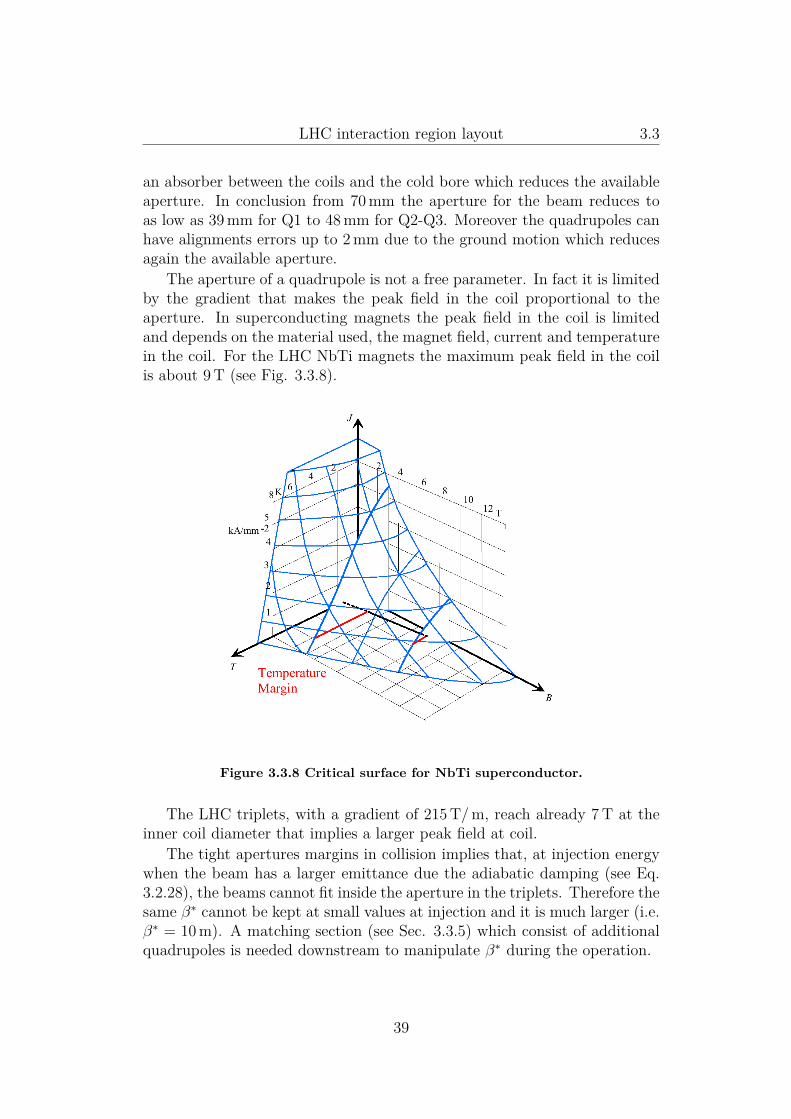
The aperture of a quadrupole is not a free parameter. In fact it is limitedby the gradient that makes the peak field in the coil proportional to theaperture. In superconducting magnets the peak field in the coil is limitedand depends on the material used, the magnet field, current and temperaturein the coil. For the LHC NbTi magnets the maximum peak field in the coilis about 9 T (see Fig. 3.3.8).
Figure 3.3.8 Critical surface for NbTi superconductor.
The LHC triplets, with a gradient of 215 T/m, reach already 7 T at theinner coil diameter that implies a larger peak field at coil.
The tight apertures margins in collision implies that, at injection energywhen the beam has a larger emittance due the adiabatic damping (see Eq.3.2.28), the beams cannot fit inside the aperture in the triplets. Therefore thesame β∗ cannot be kept at small values at injection and it is much larger (i.e.β∗ = 10 m). A matching section (see Sec. 3.3.5) which consist of additionalquadrupoles is needed downstream to manipulate β∗ during the operation.
39

LHC interaction region layout 3.3
TAS Charged particle absorberBPMSW Warm Directional Stripline for Q1MQXA Q1MCBX Cold horizontal/vertical orbit correctorBPMS Cryogenic Directional Stripline Coupler for Q2MQXB First Q2 moduleMCBX Cold horizontal/vertical orbit correctorMQXB Second Q2 moduleTASB Charged particle absorberMQSX Skew quadrupole correctorMQXA Q3MCX3 Decapole correctorMCSOX Nested skew sextupole, octupole, skew octupole correctorDFBXA Triplet FeedboxBPMSY Warm Dire:w ctional Stripline Coupler for DFBXA
Table 3.1 Elements in the triplet assembly.
The beta function gives also a measure of the sensitivities of the beamdynamics to mechanical vibrations and field imperfections. For this reasona set of corrector magnets (MC) and beam position monitors (BPM) areplaced between the main quadrupoles. Table 3.1 show the full structure.
All these elements (excluding some multipolar correctors for a reason wewill see in Sec. 5.8) must be present in all upgrade layouts.
After the matching section the beam enters the arcs. In the arcs the twobeams flow in separated magnetic channels (2-in-1 design see Fig. 3.3.9).As Beam 1 and Beam 2 have the same sign for the charge and oppositedirections, they need opposite bending fields to have their trajectory curvedin the same direction. The separation between the channel is 194 mm foralmost all the magnets (including the ones of the matching section). Thusthe two beams need to be split and recombined after the triplet. This isachieved by using the separation/recombination dipoles.
3.3.4 Separation/recombination sectionThe separation/recombination dipole section is composed of two dipoles D1and D2 with the same polarity which bend the particles of the two beam (andthe charged debris) in opposite directions (see Fig. 3.3.10 and Fig. 3.3.11).
The neutral debris will instead follow straight and an absorber calledTAN (Target absorber neutral) is needed to be put between D1 and D2. D1is composed of a set of 6 warm common bore magnet modules. They are
40

LHC interaction region layout 3.3
Figure 3.3.9 2-in-1 LHC dipole design.
Figure 3.3.10 Beam envelope at 5σ and 10σ plus tolerances for IR5 in the x− splane.
41

LHC interaction region layout 3.3
Figure 3.3.11 Beam envelope at 5σ and 10σ plus tolerances for IR1 in the y− splane.
warm because they have to sustain a high rate of radiation and heat fromthe debris. D2 is a cold 2-in-1 single dipole. It is shorter than D1 becauseD2 has a larger peak field.
The aperture required for 2-in-1 magnets can be roughly estimated withthe same arguments used for triplets as shown in Fig. 3.3.5. D1 and D2generate some dispersion that is compensated by the dispersion suppressor.D1 and D2 do not generate the crossing angle θc, for this purpose the orbitcorrector in the triplet and in the matching section are used.
In the LHC the plane of the crossing angle is vertical in IR1 and horizontalin IR5. The reason is in the cancellation of the ”pacman“ bunches effect, thatis the difference of tune between LHC bunches at edge and the core of thebunch train (see [BCL+04]).
The crossing scheme generates horizontal and vertical dispersion but itis not foreseen to be compensated. This will add to the spurious dispersioncoming from the imperfections in the arcs.
3.3.5 Matching sectionThe matching section is composed by 4 cold 2-in-1 coil quadrupoles (Q4-Q7).The quadrupoles are individually powered in order to allow flexibility in theoptics configurations. Q4 and Q5 are cooled to 4.5 K because the heat load isestimated to be larger than in the rest of the matching section, this reduces
42

LHC interaction region layout 3.4
the maximum gradient allowed in the quadrupoles. The matching sectionfrom Q4 to Q6 is well suited for an upgrade because the region is not ascomplex and crowed as the dispersion suppressor section.
Figures 3.3.12 and 3.3.13 show the arrangement of the matching sectionquadrupoles.
Figure 3.3.12 LHC IR 5 Beam 1 optics functions. The boxes represent theposition, length and polarity of the quadrupoles (blue) and dipoles (green).
3.3.6 Dispersion suppressor
The arcs generate dispersion (about 2 m) because of the dipole field. Thedispersion must be suppressed to gain aperture in the triplet and to gain lu-minosity in the IP. The dispersion suppressor uses a compact version of themissing dipole scheme and uses individually powered quadrupoles to com-pensate the not perfect match of the parameters. In the last two cells of thedispersion suppressor (Q11-Q13), the quadrupoles are powered in series withthe arc quadrupole. Individually powered trim quadrupoles (a larger one forQ11) are used to gain optics flexibility.
43

LHC interaction region layout 3.4
Figure 3.3.13 LHC IR 5 Beam 2 optics functions. The boxes represent theposition, length and polarity of the quadrupoles (blue) and dipoles (green).
3.4 Limitations of the nominal interaction re-gion layout
Chapter 2 explained how a reduction of the beam size at the IP can increasethe luminosity. This section shows what limitations arise when one tries toreduce the beam size using the existing layout.
3.4.1 ApertureThe layout of the LHC interaction region is designed to reach β∗ = 55 cm. Ifone tries to reduce β∗ to 25 cm (for σ = 11.2 µm), the required apertures inthe quadrupoles increases by a factor
√55/25 = 1.48 (see Eq. (3.3.4)). As
the divergence at the IP (γ∗ = 1/β∗) increases by reducing β∗, σ increasesproportionally to 1/
√β∗ after the IP.
One may think of reducing the emittance for reducing the beam size, butas shown in Eq. (2.3.2), the beam beam tune shift would increase accordingly,limiting the bunch intensity.
The aperture of the magnet can be increased by changing the magnettechnology (e.g. using Nb3Sn which allows a larger peak field) or decreasingthe gradient see Sec. 5.8). The last option implies longer quadrupoles asdemonstrated in Sec. 5.3.
44

LHC interaction region layout 3.4
Dxtotal Total dispersion,fspuriousdisp = 0.3 fraction of the spurious dispersion,Dmaxarc = 2 m max dispersion in the arc,βmaxarc = 180 m max beta function in the arc,fbetabeat = 0.2 beta-beating allowed in the LHCδmax energy spread in the beamxtolerances = 3 mm closed orbit tolerances
Table 3.2 Quantities for aperture estimation and values for the LHC.
Another limitation that related to the aperture is the impact of the longrange beam beam interaction. If the beam intensity is increased or operationsrequire a small tune spread, the crossing angle could be increased to reducethe effect of the long range beam beam interactions, but the aperture of thequadrupoles will not be sufficient. A possibility to solve the problem is toincrease β∗ with a loss in luminosity (including the loss due the geometricreduction factor).
In reality the beam occupies a larger region than the first estimation inSec. 3.3.3 because of machine imperfections, dispersion, orbit misalignments.A formula for a more realistic estimation of the beam size is:
Dxtotal(s) = |Dx(s)|+ fspuriousdispDmaxarc
√βx(s)βmaxarc
(3.4.1)
Dytotal(s) = |Dy(s)|+ fspuriousdispDmaxarc
√βy(s)βmaxarc
(3.4.2)
xsize(s) = fbetabeat(nσ ∗√βx(s)ε+ δmaxDxtotal(s)) + xtolerances (3.4.3)
ysize = fbetabeat(nσ ∗√βy(s)ε+ δmaxDytotal(s)) + xtolerances, (3.4.4)
where the meaning and the values of quantities appearing are explained inTab. 3.2
This formula is still not sufficient for a realistic estimation of the aperturemargin which requires a 2D aperture model ([BCL+04] and [JO97]) whichtakes into account the geometry of the beam screen and the collimationsystem.
3.4.2 Field quality and long term stabilityIf we solve the problem of the aperture in the triplet with larger magnets(using Nb3Sn for instance) the peak beta function will still increase by afactor 1/
√β∗. As discussed in Sec. 3.2.3 , the non-linear terms have an effect
45
LHC interaction region layout 3.4
which is proportional to some power of the beta function at the location of theperturbation. A larger beta requires a better field quality for the magnets.
Field quality can be improved by increasing the aperture of the quadrupoles( [BKT07]) at the cost of reducing the available gradient.
Field quality can be corrected locally by multipole corrector magnets, butthere are fundamental limitations. Firstly it is not possible to put correctorsfor each multipole because the longitudinal space requirements will be exces-sive. Usually only the multipole errors which excite the resonances close tothe machine tune are corrected (see [BFMG04]). Secondly the effects of themultipoles are weighted with the beta function ( the phase advance in thetriplet is irrelevant) and a single multipole corrector cannot cancel the con-tribution exactly. Thirdly, for common bore quadrupoles, both beams mustbe corrected at the same location, but the correction cannot be optimal forboth of them because they have different beta functions there.
3.4.3 Beam beam interactions and geometric reduc-tion factor
A reduction of β∗ at the IP implies a larger divergence of the beam whichreduces the beam beam separation in the region where the beam are in acommon beam pipe. In this case the impact of the non linear field wouldbecame unacceptable unless the crossing angle is increased. Using Eq. 3.3.5,
θc ' 450 mrad (3.4.5)
for β∗ = 25 cm if the separation is 9.8σ = dsepσ at the beam beam encounters.The increase of the crossing angle has the double effect of reducing the
luminosity and increasing the aperture requirements in the triplet. It isworth noting that the beam envelopes overlap at dsep/2(σBeam1 + σBeam2) inthe triplet if there is no orbit corrector and results in larger or smaller beambeam effect depending whether σ1 < σ2 or not (see 3.4.14).
The nominal LHC has no means (i.e wire or e-lens compensation) forcompensating the beam beam interaction which allows a smaller crossingangle or a larger currents to increase the geometric reduction factor for theluminosity. Alternatively crab cavities can rotate the beam in order to forcehead on collisions (no geometric reduction factor) allowing a larger crossingangle which would allow more current but would require additional aperturein the quadrupoles.
46

LHC interaction region layout 3.4
Figure 3.4.14 Beam beam separation for the nominal LHC. The lines showthe separation of the centroids of the beams in multiples of σ. Every 3.75 mthere are long range beam beam interactions (lrbb) that are negligible whenthe separation of the beam is larger than 12σ. The separation is not constantand the location where the interactions occurs at small distance are dominantfor the beam dynamics.
47

LHC interaction region layout 3.4
3.4.4 Heat depositionWith an upgrade of the luminosity, the rate of debris generated by beamcollisions at IP increases accordingly. The LHC absorbers (TAN and TAS)are designed to reduce the heat load in the superconducting magnet for thenominal luminosity. In case of a luminosity upgrade either the absorbermust be redesigned, or the superconducting magnets must be able to sustaina higher heat load or the aperture of magnet must be increased in order notto intercept the debris.
3.4.5 Radiation damageThe debris generated at the IP are not only responsible for the heat load,but also for the radiation damage. The LHC triplets lifetime is estimated tobe 700 fb−1 of integrated luminosity which translates into 7 years of opera-tion. The radiation damage must be carefully addressed in order to keep thelifetime of the magnets reasonably high.
3.4.6 Chromatic aberrationsAs for the long term stability, an increase of the beta function increases thechromatic aberrations. They are responsible for tune dependence on the en-ergy which can enhance the excitation of the resonances and the instabilities.
The linear part must be corrected by the lattice sextupoles. The nonlinear part is difficult to correct and can drive instabilities and as well decreasethe efficiency of the collimation.
3.4.7 MatchabilityIn order to create a small β∗, the beta function at the triplet must be large,but the arcs require a smaller beta. The matching section and dispersionsuppressor must therefore be able to transform a small beam with smalldivergence in the arc into beam with a large divergence in Q4 in order toassure a large beta in the triplet.
If too large beta values are required, the LSS magnets may be limitedin strength and aperture. The LSS must also be able to change the opticsconfiguration smoothly between small β∗ optics for collision and large β∗optics for injection and ramping at a constant phase advance. Although thenumber of parameters (individually powered quadrupoles) is larger than thenumber of constraints, the magnets are often at the limit of their strengths.In addition not all parameters are truly independent or efficient. For instance
48

LHC interaction region layout 3.5
for controlling the βy only the quadrupole for which βy >> βx are efficientor quadrupoles where Dx is large are better for changing the dispersion. Thequadrupoles must be placed at different phases such that they can controlindependently several parts of the optics.
3.5 ConclusionIn this chapter I showed the basic tools for studying the transverse beamdynamics. The transverse beam dynamics is an essential tool for studyingthe interaction region layout. An analysis of the limitations of IR arisingwhen one tries to reduce the beam size at the IP introduced the main topicfor the design of an interaction region upgrade.
The following chapters develop two different upgrade strategies trying toaddress and surpass the limitations discussed before. Chapter 4 studies adipole first layout, an option which inverts the position of the triplets withthe separation recombination dipoles. Chapter 5 studies several low gradientquadrupole first layouts in which large aperture and longer quadrupoles areused to overcome the aperture limitation of the present layout.
49

LHC interaction region layout 3.5
50
Chapter 4
Dipole first layout
4.1 IntroductionIn this chapter I discuss the dipole first layout. The advantages and draw-backs are analized by studing a realistic layout.
4.2 MotivationsAs discussed in Ch. 3, some of the limitations of the LHC interaction regionare:
• long range beam beam interactions (see Sec. 3.4.3 )
• heat deposition and radiation damage (see Sec. 3.4.4 and 3.4.5)
• correction of field imperfections (see Sec. 3.4.2 and 3.2.3)
Dipole first options try to overcome these limitations by exchanging theposition of the triplet and the separation/recombination magnets with re-spect to the nominal layout.
Dipole first layouts have been proposed first in [BCG+02]. Further stud-ies can be found in [dM05], [SSM05], [Bru05], [dMBR06], [SJM+06], and[SJRT07].
In the following I develop a dipole first layout in order to check its fea-sibility in terms of linear optics, field quality specifications, aberrations andlong term stability.
51
Dipole first layout 4.3
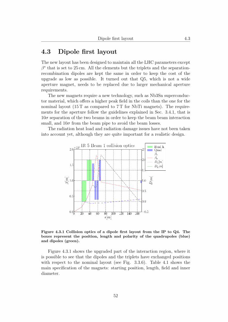
4.3 Dipole first layoutThe new layout has been designed to maintain all the LHC parameters exceptβ∗ that is set to 25 cm. All the elements but the triplets and the separation-recombination dipoles are kept the same in order to keep the cost of theupgrade as low as possible. It turned out that Q5, which is not a wideaperture magnet, needs to be replaced due to larger mechanical aperturerequirements.
The new magnets require a new technology, such as Nb3Sn superconduc-tor material, which offers a higher peak field in the coils than the one for thenominal layout (15 T as compared to 7 T for NbTi magnets). The require-ments for the aperture follow the guidelines explained in Sec. 3.4.1, that is10σ separation of the two beams in order to keep the beam beam interactionsmall, and 10σ from the beam pipe to avoid the beam losses.
The radiation heat load and radiation damage issues have not been takeninto account yet, although they are quite important for a realistic design.
Figure 4.3.1 Collision optics of a dipole first layout from the IP to Q4. Theboxes represent the position, length and polarity of the quadrupoles (blue)and dipoles (green).
Figure 4.3.1 shows the upgraded part of the interaction region, where itis possible to see that the dipoles and the triplets have exchanged positionswith respect to the nominal layout (see Fig. 3.3.6). Table 4.1 shows themain specification of the magnets: starting position, length, field and innerdiameter.
52
Dipole first layout 4.4
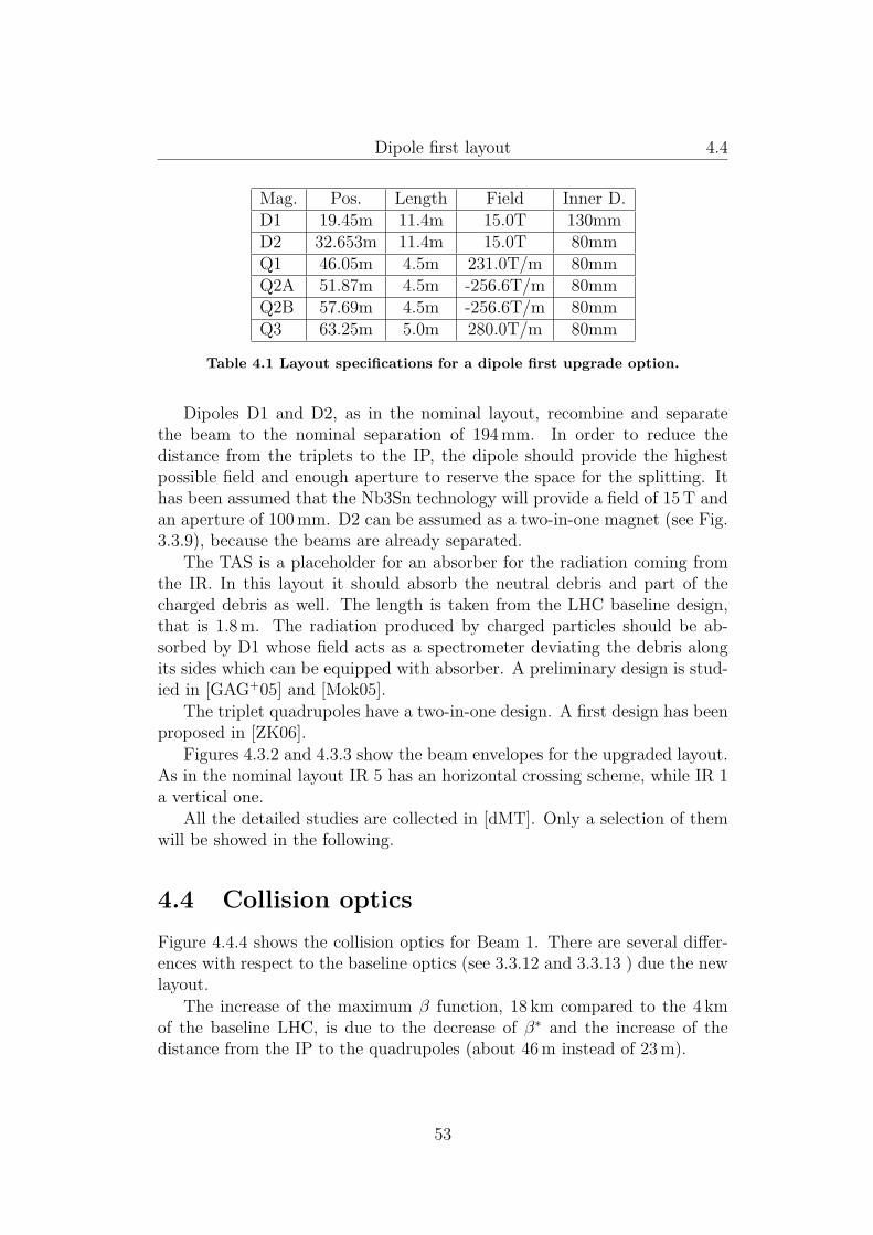
Mag. Pos. Length Field Inner D.D1 19.45m 11.4m 15.0T 130mmD2 32.653m 11.4m 15.0T 80mmQ1 46.05m 4.5m 231.0T/m 80mmQ2A 51.87m 4.5m -256.6T/m 80mmQ2B 57.69m 4.5m -256.6T/m 80mmQ3 63.25m 5.0m 280.0T/m 80mm
Table 4.1 Layout specifications for a dipole first upgrade option.
Dipoles D1 and D2, as in the nominal layout, recombine and separatethe beam to the nominal separation of 194 mm. In order to reduce thedistance from the triplets to the IP, the dipole should provide the highestpossible field and enough aperture to reserve the space for the splitting. Ithas been assumed that the Nb3Sn technology will provide a field of 15 T andan aperture of 100 mm. D2 can be assumed as a two-in-one magnet (see Fig.3.3.9), because the beams are already separated.
The TAS is a placeholder for an absorber for the radiation coming fromthe IR. In this layout it should absorb the neutral debris and part of thecharged debris as well. The length is taken from the LHC baseline design,that is 1.8 m. The radiation produced by charged particles should be ab-sorbed by D1 whose field acts as a spectrometer deviating the debris alongits sides which can be equipped with absorber. A preliminary design is stud-ied in [GAG+05] and [Mok05].
The triplet quadrupoles have a two-in-one design. A first design has beenproposed in [ZK06].
Figures 4.3.2 and 4.3.3 show the beam envelopes for the upgraded layout.As in the nominal layout IR 5 has an horizontal crossing scheme, while IR 1a vertical one.
All the detailed studies are collected in [dMT]. Only a selection of themwill be showed in the following.
4.4 Collision opticsFigure 4.4.4 shows the collision optics for Beam 1. There are several differ-ences with respect to the baseline optics (see 3.3.12 and 3.3.13 ) due the newlayout.
The increase of the maximum β function, 18 km compared to the 4 kmof the baseline LHC, is due to the decrease of β∗ and the increase of thedistance from the IP to the quadrupoles (about 46 m instead of 23 m).
53

Dipole first layout 4.4
Figure 4.3.2 Beam envelope at 5σ and 10σ plus tolerances for IR 5 in the x− splane. The red and blue lines show the crossing angle in the horizontal plane.
Figure 4.3.3 Beam envelope at 5σ and 10σ plus tolerances for IR 1 in the y− splane. The red and blue lines show the crossing angle in the vertical plane.
54

Dipole first layout 4.5
Figure 4.4.4 Collision optics for Beam 1 in IR 5 for the dipole first layout.
In the matching region (Q4-Q7) the dispersion (see Sec. 3.2.4) is notzero. This is due to the fact that D1-D2 introduce a dispersion bump thathas to be compensated in order to get a zero dispersion at the IP. Dispersionin this region reduces the degrees of freedom of the matching quadrupoles.The dispersion suppressor quadrupoles have to be used for the matchingpurposes. Moreover the dispersion breaks the symmetry between left andright with respect to the IP and the symmetry between Beam 1 and Beam2, making the optics solution slightly different for each of these regions.
4.5 Crossing schemeA crossing angle different from zero is needed for the LHC in order to limitthe long range beam-beam interactions between the two beams.
The dipole first layouts reduces the number of LRBB to 5 from 15 of thenominal LHC. See Fig. 4.5.5 compared with Fig. 3.4.14.
The value of the angle depends on the separation needed to reduce thelong range beam beam interaction (see Sec. 3.4.3, 3.3.1, and 2.3.4). Forthis layout it has been assumed the same separation in σ that is present inthe nominal layout. In these conditions, the reduced number of long rangebeam beam interaction allows a large bunch intensity and therefore a largeluminosity with respect to the nominal.
Table 4.2 shows the values of the crossing angles needed for the base-
55

Dipole first layout 4.5
Figure 4.5.5 Beam beam separation for the dipole first layout.
Data Unit LHC Upg.Energy [GeV] 7000 7000Relativistic gamma 7461 7461Normalized emmittance [µm rad] 3.750 3.750Emmittance (ε) [nm rad] 0.503 0.503RMS beam size at IP [µm] 16.63 11.21Half crossing angle (φ) [µrad] 142.5 211.4Half separation (d) [σ] 4.714 4.714
Table 4.2 Data used for estimating the required crossing angle for the nominalLHC and dipole first layout.
line LHC and dipole first layout LHC in order to fulfill the required beamseparation.
The crossing scheme is managed by D1 and D2 and by orbit correctors asin the nominal layout. This is a great advantage because reduces the apertureneeds of the triplet magnets and does not introduce spurious vertical andhorizontal dispersion. In the LHC the vertical dispersion cannot be correctedand the spurious dispersion propagates in the rest of the machine.
Figures 4.5.6 and 4.5.6 show the crossing schemes for the horizontal andvertical plane. The former can be achieved with a slightly different bendingangle for D1 and D2 and the latter by tilting D1 and D2 resulting in avertical deflection. The dispersion kicks compensate exactly because there is
56

Dipole first layout 4.6
no quadrupole in between.
Figure 4.5.6 Crossing scheme for IR 1 Beam 1 before collision. The lines showthe horizontal and vertical displacement of the closed orbit of Beam 1. Inthe vertical plane the Beam 1 cross the IP with a crossing angle, while in thehorizontal plane the beam is displaced to avoid collision with the other beam.During collision the horizontal displacement is removed and the beam collideswith a vertical crossing angle.
A separation at the IP is also needed during the injection and the accel-eration of the particles. It can be achieved either using the orbit correctormagnets or dividing D1 and D2 in two parts and powering them differently.
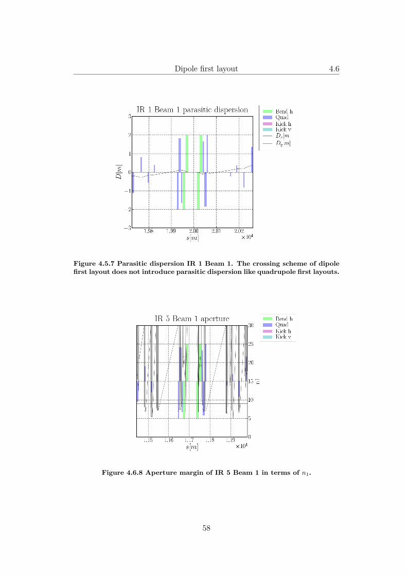
Figures 4.5.7 and 4.5.7 show the dispersion function when the crossingangle scheme is on and demonstrate that there is no mismatch outside theinteraction region.
4.6 Mechanical apertureFigure 4.6.8 shows the mechanical aperture in term of n1 (see [JO97]) forthis optics. An acceptable value for n1 in the LHC is 7σ. The figure showsthat Q5, due to the high β values, needs a bigger aperture. The high valuesof β are unavoidable due the layout, therefore an upgrade of Q5 to a wideaperture quadrupole (e.g. like an MQY) is necessary.
57
Dipole first layout 4.6
Figure 4.5.7 Parasitic dispersion IR 1 Beam 1. The crossing scheme of dipolefirst layout does not introduce parasitic dispersion like quadrupole first layouts.
Figure 4.6.8 Aperture margin of IR 5 Beam 1 in terms of n1.
58

Dipole first layout 4.7
4.7 ChromaticityAt collision energy, the chromaticity of the LHC (see Sec. 3.2.4 and Sec.3.4.6 ) is dominated by natural chromaticity of the triplet quadrupoles.
The LHC uses lattice sextupoles for correcting the chromaticity. For eachof the 8 arcs in the LHC there are:
• two focusing sextupoles families (Bmax = 1.280T at 17mm),
• two defocusing sextupoles families (Bmax = 1.280T at 17mm),
• one spool piece sextupoles family (Bmax = 0.471T at 17mm).
These elements can be used for correcting the first and second order chro-maticity and the off-momentum beta-beat. Their impact on the long termstability is minimized because they are interleaved and at π phase advance.
Figures 4.7.9 and 4.7.10 show the chromaticity and the off momentumbeta beat after correction. The first order chromaticity is corrected by thechromatic sextupoles. The second order chromaticity together with the off-momentum beta beat in the triplet and in the half of the machine is correctedby a correct phasing of the IRs as indicated in [Far99].
Figure 4.7.9 Chromatic change of the tune for the dipole first layout. The nonlinear terms are much stronger with respect to the nominal values.
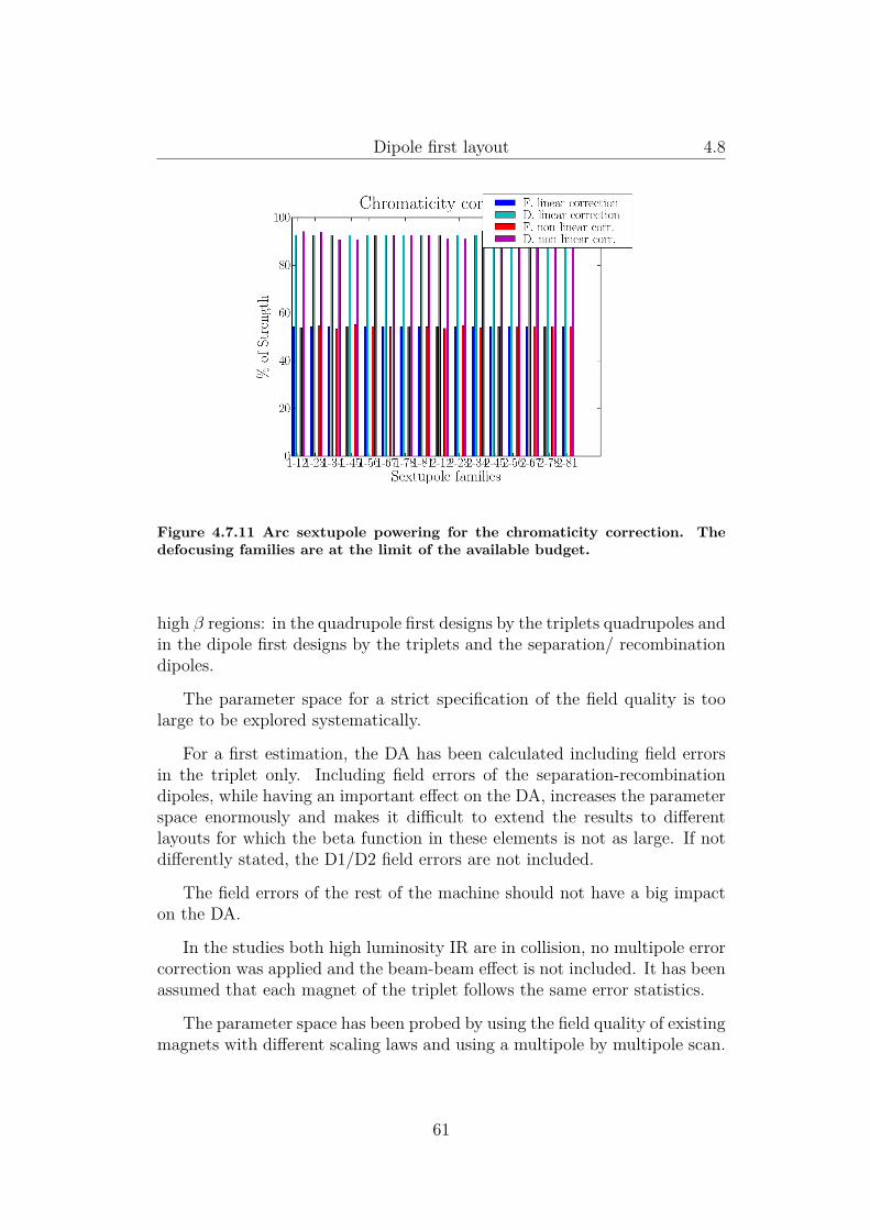
Figure 4.7.11 shows the percentage values of the arc sextupoles requiredfor the chromaticity correction. The defocusing values are bigger than the
59

Dipole first layout 4.8
Figure 4.7.10 Chromatic beta-beating at δ = 3 · 10−4 for the dipole first layout.The beta-beating is four times larger with respect to the nominal values.
focusing one because the dispersion is smaller in the location in which theyare placed. They use all the available budget.
An attempt to correct the chromaticity (see [dMBR06]) with local sex-tupoles in the triplet failed due to the large geometric aberrations arisingfrom the strong sextupolar field required for the correction. These compo-nents could be compensated by another set of families located where disper-sion vanishes and at π phase advance, but there are no suitable places fortheir installation. The sextupolar field in the triplet can be reduced by alocal increase of the dispersion, but the non-linear dispersion emerging fromthe process spoils the efficiency of the local compensation.
4.8 Dynamic apertureThe dynamic aperture (DA) is estimated by tracking an off-momentum (δ =0.27 · 10−3) particle distribution 105 turns in 60 realizations of the machineusing a statistical model of the multipole field error distribution. The min-imum DA among the 60 realizations should give the real dynamic apertureof the machine within a factor of 2 (see the LHC design report [BCL+04]).A simulated DA of 12σ is therefore satisfactory because the beam-beam in-teractions and the collimators will limit the aperture to 6σ anyway.
At collision the DA is dominated by the field quality of the elements in the
60
Dipole first layout 4.8
Figure 4.7.11 Arc sextupole powering for the chromaticity correction. Thedefocusing families are at the limit of the available budget.
high β regions: in the quadrupole first designs by the triplets quadrupoles andin the dipole first designs by the triplets and the separation/ recombinationdipoles.
The parameter space for a strict specification of the field quality is toolarge to be explored systematically.
For a first estimation, the DA has been calculated including field errorsin the triplet only. Including field errors of the separation-recombinationdipoles, while having an important effect on the DA, increases the parameterspace enormously and makes it difficult to extend the results to differentlayouts for which the beta function in these elements is not as large. If notdifferently stated, the D1/D2 field errors are not included.
The field errors of the rest of the machine should not have a big impacton the DA.
In the studies both high luminosity IR are in collision, no multipole errorcorrection was applied and the beam-beam effect is not included. It has beenassumed that each magnet of the triplet follows the same error statistics.
The parameter space has been probed by using the field quality of existingmagnets with different scaling laws and using a multipole by multipole scan.
61

Dipole first layout 4.8
4.8.1 DA from measured errorsThe present magnet production is used as a reference for the field qualityin the tracking studies. The present MQXB is used as prototype for a highgradient quadrupole and the present MQY is used as prototype for a largeaperture quadrupole.
Two different scaling laws for the multipole errors are applied. The firstis a uniform scaling. The second is expressed by the equation
bn(d1) = (d0/d1)nbn(d0), (4.8.1)where bn(d1) is the relative multipole error of order n (n = 0 is a dipole) fora magnet of aperture d1 and the bn(d0) is the relative multipole error for amagnet of aperture d0. The reference radius of bn(d1) and bn(d0) is the same.This equation (see [BKT07]) takes into account the geometric scaling of therelative multipoles and the coil precision which does not scale.
Figure 4.8.12 Triplet field quality used for the tracking studies. It is equivalentto the present production of the MQXB. The resulting DA is 3σ. If the errorsare scaled uniformly by 10%, the resulting DA is 8.3σ.
Figures 4.8.12, 4.8.13, 4.8.14 show the field quality used for several track-ing studies and the resulting DA.
4.8.2 Multipole by multipole analysisAn upper bound on the minimum DA can be found by probing one multipoleerror at the time.
62

Dipole first layout 4.8
Figure 4.8.13 Triplet field quality used for the tracking studies. It is equivalentto the present production of the MQY scaled by Eq. 4.8.1. The resulting DAis 2σ.
The DA follows a simple scaling law (see [Zie95]) when there is a singlemultipole error in a machine:
log(dn) ∼ −1
n− 2 . (4.8.2)
where dn is the DA in terms of sigma due field errors of order n.Figure 4.8.15 and 4.8.16 show the dependence of the DA from the mul-
tipole strength where the multipole strength is expressed in term of relativemultipole error at two different reference radius.
The curves reproduce the theoretical scaling law. The plot looks morenatural when the reference radius is 12σ ' 34mm.
The multipoles b6, b8, b10 are dominant and the same effect is observedin the simulation for the nominal LHC.
A tracking study where all the multipoles are set to 1 unit at 34 mm ref-erence radius has been performed and the results shows that the combinationof the effects of the single multipoles lead to a DA of 4.5σ.
As comparison the DA of the nominal LHC without multipole error cor-rection is 14σ.
The results presented here demonstrated that this dipole first layout hasan extreme sensitivity to the field quality of the triplet. The specification ofthe required field errors are beyond the technology reach. Even an efficient
63

Dipole first layout 4.8
Figure 4.8.14 Separation recombination dipole field quality used for the track-ing studies. It is equivalent to the present production of the cold D2. Thetriplets has the field quality of the MQXB as showed in Fig. 4.8.12. Theresulting DA is 0.8σ. If the errors are scaled uniformly by 10%, the resultingDA is 6σ.
corrector package allowed by the separated magnetic channel of dipole firstlayouts will hardly compensate the field error and bring the DA to acceptablelevels.
64

Dipole first layout 4.8
Figure 4.8.15 DA when only a multipole is active as function of the multipoleerrors.The reference radius is 17mm.
Figure 4.8.16 DA when only a multipole is active as function of the multipoleerrors.The reference radius is 34mm.
65

Dipole first layout 4.8
Figure 4.8.17 Triplet field quality used for the tracking studies. It is equivalentto 1 unit at 34mm reference radius. The resulting DA is 4.5σ.
66
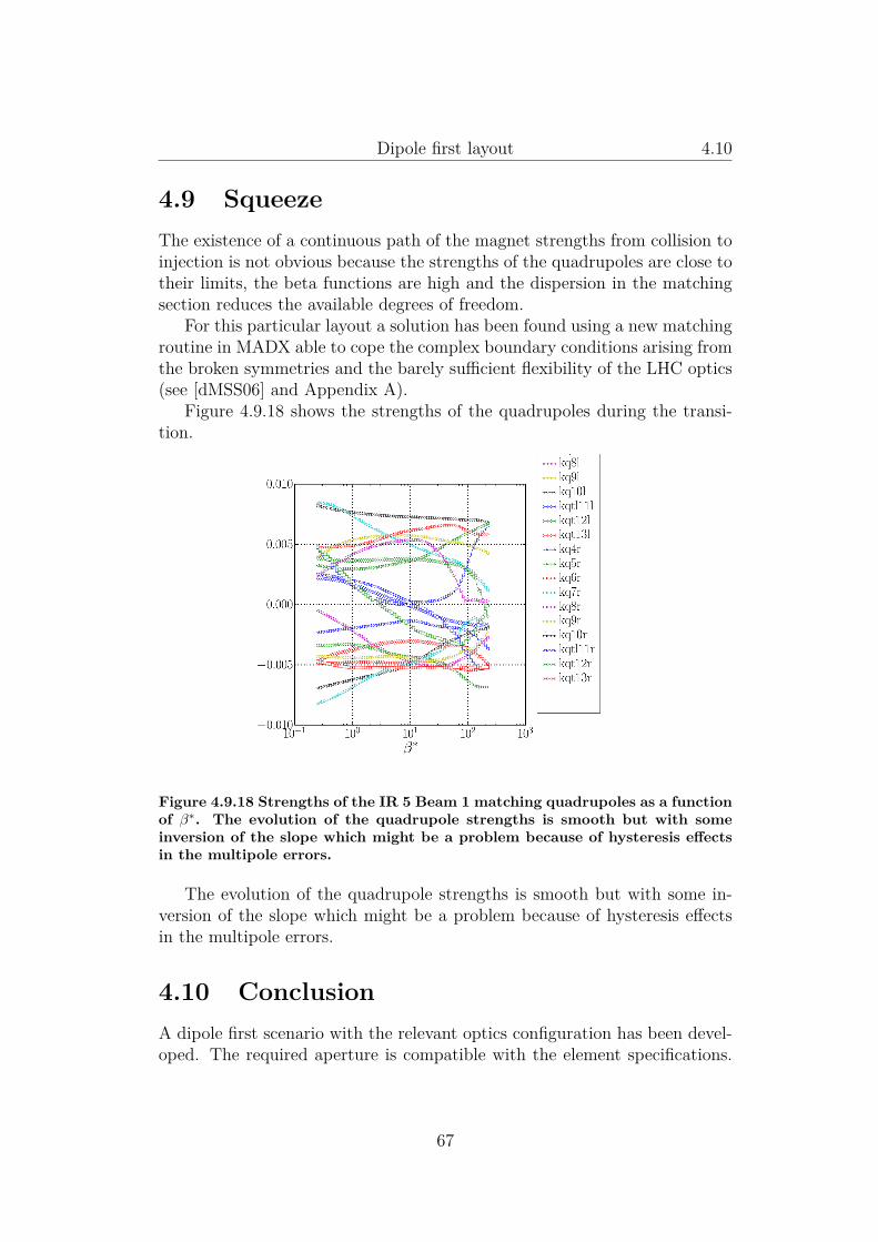
Dipole first layout 4.10
4.9 SqueezeThe existence of a continuous path of the magnet strengths from collision toinjection is not obvious because the strengths of the quadrupoles are close totheir limits, the beta functions are high and the dispersion in the matchingsection reduces the available degrees of freedom.
For this particular layout a solution has been found using a new matchingroutine in MADX able to cope the complex boundary conditions arising fromthe broken symmetries and the barely sufficient flexibility of the LHC optics(see [dMSS06] and Appendix A).
Figure 4.9.18 shows the strengths of the quadrupoles during the transi-tion.
Figure 4.9.18 Strengths of the IR 5 Beam 1 matching quadrupoles as a functionof β∗. The evolution of the quadrupole strengths is smooth but with someinversion of the slope which might be a problem because of hysteresis effectsin the multipole errors.
The evolution of the quadrupole strengths is smooth but with some in-version of the slope which might be a problem because of hysteresis effectsin the multipole errors.
4.10 ConclusionA dipole first scenario with the relevant optics configuration has been devel-oped. The required aperture is compatible with the element specifications.
67

Dipole first layout 4.10
Q5 should be replaced with an MQY magnet type. The crossing schemes arecompletely managed by D1/D2 and there is no dispersion mismatch due thecrossing angle.
The linear and second order chromaticity can be corrected by the sex-tupoles in the arcs. The third order chromaticity poses a limit for theoperational margins (i.e. chromaticity measurement). The off-momentumbeta-beat is under control in the triplet but not in the arc. It should bepossible to compensate it using the available budget of sextupole strength.
The field quality of the present magnet production alone cannot assurethe required DA. The better field quality expected from a large aperturedoes not help. b3 seems responsible for the lowest DA but scales quickly.b6, b8, b10 scale slowly and might represent a bottle neck. The multipoleerrors should be smaller than 1 unit at 34mm for upgrade scenarios where themaximum beta function is larger than 18km. An effective corrector packageis needed to reach the required DA.
The radiation damage due the debris has not been addressed yet. Thelayout allows a natural magnetic TAS (racetrack magnets) for the chargeddebris. It is not clear how to cope with neutral debris.
In conclusion the dipole first layout studied, while assuming an optimisticimprovement of the magnet technology, requires extremely tight field qualityspecification in order to preserve the long term stability. The chromatic aber-rations are just on the limit of ability to correct them and high order termsmay reduce the performance of the LHC. The layout assumes optimisticallythat the heat load and radiation damage can be reduced by an optimizedprotection systems whose feasibility has not demonstrated yet.
For these reasons the dipole first options has been considered too challeng-ing to implement in practice . In order to make a comparison, the followingchapter will study quadrupole first options whose main driving criteria is thetechnical feasibility using the existing technology.
68

Chapter 5
Quadrupole first layouts
5.1 IntroductionIn this chapter I discuss quadrupole first layout options. I developed andused an analytical tool for a parameter survey of the performance of thequadrupole first layout options and for designing optimized layouts. I studieddifferent realistic layouts that are designed to address different design criteria.The advantages and drawbacks of quadrupole first options are analyzed bystudying the performance of the layouts.
5.2 MotivationAs discussed in the Ch. 3 some of the limitations of the nominal interactionregion are:
• aperture limitations (see Sec. 3.4.1);
• heat deposition and radiation damage (see Sec. 3.4.4 and 3.4.5);
• field quality (see Sec. 3.4.2 and 3.2.3);
Quadrupole first layout options try to overcome these limitations by usinglonger and weaker magnets requiring magnets compatible with the existingtechnology.
5.3 Optimization of triplet layoutThe design of quadrupole first layouts requires a careful optimization of thefocusing system assembly.
69

Quadrupole first layouts 5.3
First results (see [dMB06]) gave an indication that weaker and longermagnets can fulfill the requirements of the upgrade with existing magnettechnology.
However, these type of layouts enhance the chromatic effect and integra-tion issues with the matching section, which are already enhanced by thereduction of β∗, because the beta function in the triplet becomes larger ascompared to focusing systems which uses short and stronger magnets.
Therefore, it is important to find the final focus layouts which minimizethe beta function in the quadrupoles. At this stage of the design, it is alsoimportant to identify the theoretical limitations in order to ensure that thefound solutions are optimal and also for giving directions to technology R&D.
The analysis that follows is not limited to triplets only, but tries to studymultiplets with any number of quadrupoles. From now on I will call finalfocus system the set of magnets that focus the beam before the collisionpoint. In this sense the LHC triplets are a final focus system.
Several papers and reports have been written on the design and opti-mization of quadrupole multiplets topic, see [Reg67a], [Reg67b]. Althoughthe results are useful as calculation tools for the analysis of a layout (in par-ticular when the computational resources were limited), they are not suitedfor the design process of a final focus system for the LHC due to the complex-ity of the formulas which relate the layout parameters with the performancegoals.
An approach, used in particular for linear collider by taking advantage ofthe symmetries in the layout and using thin lens approximation, (e.g. [BS84],[BS87] and more recently [RS01]) allows to optimize the chromatic and ge-ometric aberrations by using non-linear elements and to achieve very smallspot size, but leads to longer and more complex structures compared to theones involving only linear elements. In circular colliders, this approach hasnot been yet proved to be satisfactory due to the space limitations which donot allow efficient layouts and to a non-exact cancellation of the aberrationswhich limits the dynamic aperture (see [dMBR06]).
Other studies used several approximations (e.g. thin lens approximationin [dG97] and [dG98] ) and restricted the analysis to some particular cases(e.g. coarse parameter scan for the SSC in [Peg84] or symmetric triplets forthe LHC in [dG97], [dG98] and [KRT07]) in order to decrease the complexityof the equations and reduce the dimensionality of the parameter space. Thisstrategy exposes the studies to the chance of missing the true optimum anddoes not answer the question of what are the limitations induced by a magnettechnology independently on the details of a given layout. In fact, the thinlens approximation is not always accurate and usually requires a refinementusing the exact thick lens theory that spoils the generality of the results.
70

Quadrupole first layouts 5.3
A symmetric triplet is a layout that offers good performance (e.g. in thenominal LHC), but not in all possible scenarios.
We will now see how to write the equations needed to solve for designingan optimized final focus systems.
5.3.1 Final focus designFinal focus systems are supposed to invert the sign of the divergence of thebeam (x′(s) and y′(s)) which tends to defocus the beam when it is seencoming from the IP.
In terms of Twiss parameter the focusing system must invert the sign of αin both plane. The exact values for α at the of the final focus system dependson the peak beta function and the position and aperture of the quadrupolesin the matching section.
The conditions for α translate in two equations. These equations can berelaxed in inequalities, assuming that the matching section will be able toabsorb a range of values. For the LHC this assumption is weak for the reasondiscussed in Sec. 3.4.7.
Initial conditions
The design of a final focus system starts from the definition of the initialcondition in the IP. Section 2.3 shows that the transverse beam sizes atthe IP of the colliding beams must be equal for maximizing the luminosity.The transverse beam sizes at the IP depends on the vertical and horizontalemittance and vertical and horizontal beta function.
Hadron machines exhibits the same emittance in both planes becausethere is no strong natural mechanism that affect the emittance in one partic-ular plane, as opposed to lepton machines where the synchrotron radiationdamps the motion only in the horizontal plane. It implies that both beamsmust have the same beta functions.
Section 2.3.4 shows that elliptical beams optimize the luminosity, but itis not easy to generate elliptical beams using quadrupole first layouts in theLHC. The reason is that the region occupied by the beam must be as roundas possible to use efficiently the round aperture of the quadrupole. In caseof quadrupole first layouts both beam uses the same quadrupole field, butas the charge is the same but the momentum opposite, the two beams willexperience opposite force. For instance, if a quadrupole is focusing for Beam1 in the one plane, it will be defocusing for Beam 2 in the opposite plane.This symmetry implies that if one optimize the aspect ratio of Beam 1 tobe round in the triplet and elliptic in the IP, it will automatically distort
71

Quadrupole first layouts 5.3
Beam 2 that will not be optimized as well. Only round beams at the IPoptimize the aperture of the quadrupole. There is then a trade off betweenthe ellipticity that optimize the luminosity and the roundness that optimizesthe aperture. For the LHC, the particular shape of the beam screen whichhas not a circular symmetry allow an optimization of both the aperture andthe luminosity as shown in [Far09] using slight elliptic beams.
In conclusion optimized layouts should generate round beams with thesame beta function in both planes, therefore in the literature it is commonto refer to β∗ has a single quantity.
Minimizing the peak beta function
For finding the layout that minimizes the peak β function with the limita-tion that the peak field in the coil is fixed, it would be necessary to havemagnets whose aperture and gradient be a continuous function of s. This isnot possible for technological reasons, therefore we have to assume that thegradient and the aperture are fixed within a magnet module.
In order to generate round beam, final focus system must provide ap-proximately the same focusing strength in both planes. Only a set of threeor more quadrupoles can guarantee equal focusing properties in both planes,therefore we will concentrate on multiplets with a number of quadrupoleslarger than 3.
This assumption simplifies the optimization problem, but it would requiredifferent magnets with different cross sections. For cost reasons in terms ofR&D and spare policies , it would be better to use magnet with the sameaperture, the same gradient and the same length. In this way the number ofparameters reduces and the effectiveness of the optimization reduces as well.In the rest of the chapter we will see several options with different balancesof modularity and optimizations.
Using these assumptions the optimization problem translates in imposingthat the peak of the beta functions and the absolute value of the gradientwill assume all the same value. In this way all the quadrupoles will exercisethe all the available focusing leverage because the edge of the beam will seealways the maximum bending field. The number of peak of the beta functiondepends on the number of quadrupoles in the multiplets. For triplets thepeaks are 2 because the beam should see a bending field of opposite polarityin two planes (see Fig. 5.3.2). For quadruplets the number of peaks are 3and so on.
The requirements for optimization translate in n − 2 equations where nis the number of quadrupoles.
72

Quadrupole first layouts 5.3
5.3.2 ParametersIn conclusion for a given multiplet optimization we have n+1 equations andn+1 parameters. The parameters are n lengths of the quadrupoles li and thenormalized gradient k. The layout equations depend on the initial conditionL∗, β∗, which determine the boundary conditions for the Twiss parametersat the beginning of the final focus system. The final conditions for α atthe end of the final focus system represent other two parameters. Howevertheir values are extremely difficult to specify because they depend on theability of the matching section to manipulate the beta function using thestrengths of the quadrupole (20 parameters in total) while being compatiblewith the hardware constraints. No study has been done yet to clearly specifythose conditions, because the set of allowed values of the matching sectionparameter strengths has the form of not connected hyper surfaces of a largenumber of dimensions.
In order to continue the general treatment we assume that at the bound-ary of the final focus αx = αy = 0. In other words we will now look for pointto parallel final focusing systems, where the point is the IP and the beamtrajectories are become parallel after the focus system. These hypothesisallow us to find the minimum beta function that a final focus can achievein theory. Any focusing boundary conditions for which α > 0 will resultsin a larger peak function because the quadrupoles must focus more, thus belonger (the peak field is fixed) thus they defocus more in the other plane andthey make the peak beta grow.
Another simplifying hypothesis is to leave no empty space between thequadrupoles. While technologically impossible, the hypothesis allow a gen-eral treatment of the problem. As additional drift spaces result in an in-crease of the beta function, gap-less final focus system will always featuresthe smallest possible beta peaks.
Using gap-less parallel to point focusing system the problem depends nowonly on β∗, L∗, k(s) and the quadrupoles lengths li.
5.3.3 Approximation of the equationsAs explained in Sec. 3.2.2, Eq. 3.2.14 or Eq. 3.2.16 can be used to find thedependance of the beta functionon the focusing properties of a lattice k(s).There are several analytical and numerical methods for solving this equationusing a matrix approach (see for instance [CT99]). The challenge is to findparameter dependent solutions.
A full analysis of the problem can be found in [dM07a] and referencetherein. The strategy explained and adopted in this paper use a well justi-
73

Quadrupole first layouts 5.3
fied approximation that simplifies the equations and allows write the problemin dimensionless quantities. The dimensionless problem can be solved numer-ically and the actual quantities can be scaled back.
In the following part I sketch the main passages.Let wx =
√βx and wy =
√βy, then using Eq. 3.2.16:
w′′x(s) + k(s)wx(s)−1
w3x(s)
= 0 (5.3.1)
w′′y(s)− k(s)wy(s)−1
w3y(s)
= 0, (5.3.2)
where k(s) is the normalized quadrupole strength and the sign changes de-pending on the plane.
In a final focus system, the high order term can be neglected because1/w3 is often a small number compared to the variation of w over s andk(s)wx(s) in a focus system. Last equations (Eq. 5.3.1 and 5.3.2 ) assumethe form of
w′′(s)± k(s)w(s) = 0 (5.3.3)
and, if k is constant, a solution has the form of
w(s) = w0 cos(s√|k|) + w′0√
|k|sin(s
√|k|) (5.3.4)
or
w(s) = w0 cosh(s√|k|) + w′0√
|k|sinh(s
√|k|) (5.3.5)
, depending on the sign of ±k(s).A first application allows to find the maximum of β inside a focusing
quadrupole. If the approximation is valid and if this maximum is not triviallyon one of the two extremities, the maximum β in a quadrupole can be foundsolving the system:
wm = w(sm) = w0 cos(sm√|k|) + w′0√
|k|sin(sm
√|k|) (5.3.6)
0 = w′(sm) = −w0
√|k| sin(sm
√|k|) + w′0 cos(sm
√|k|). (5.3.7)
74

Quadrupole first layouts 5.3
which is equivalent to
tan(sm√|k|) = w′0
w0
√|k|
= − α0
β0
√|k|
(5.3.8)
βm = w2m = w2
0 + w′0√|k|
2
= β0 −α0
β0k(5.3.9)
where βm = w2m is the maximum β, sm is the location where the maximum
occurs, w0 =√β0 and w′0 = −α0/w0 are the initial conditions at the begin-
ning of the quadrupole.
5.3.4 NormalizationWe can now define dimensionless quantities θ, w(θ) defined by
θ = s√|k| w(s) = w(θ) w′(θ = 0) = 1 (5.3.10)
In this case Eq. 5.3.1 and 5.3.2 become:
w′′(θ) + k(θ)w(θ) = 0, (5.3.11)
where k(θ) = ±1 depending whether at θ there is a focusing or defocusingquadrupole and the solution are a series of circular and hyperbolic rotations(see for instance Fig. 5.3.1).
As Eq. 5.3.11 is linear and homogeneous, the solution depends only onthe ratio of the initial conditions that is
w0/w′0 =
√|k|w(L∗)/w′(L∗) = L∗
√|k| (5.3.12)
, because
w(L∗) = L∗/√β∗ w′(L∗) = 1/
√β∗ (5.3.13)
.
5.3.5 ScalingsUsing this property we can solve the optimization problem using the initialconditions w′0 = 1 and varying w0 from 0 to ∞ and use
L∗√|k| = w0 (5.3.14)
w(s) = w(θ)√β∗√|k| (5.3.15)√
|k|li = θi, (5.3.16)
75

Quadrupole first layouts 5.3
Figure 5.3.1 Phase space diagram for a point to parallel constant gradienttriplet with initial condition w0 = sin(θ0), w′0 = cos(θ0), θ0 = π/4. The curvesshow w =
√β in the (w,w′) space. The black curve (x) is composed by a
sequence of a circular, hyperbolic and again circular rotation which representsa sequence of a focusing, defocusing and again focusing quadrupole. The redcurve on the contrary (y) is composed by a hyperbolic, circular and hyperbolicrotations. The circular rotation for the y coordinate and the last circularrotation for x on the right side of the figure overlaps because one has imposedthat max(βx) = max(βy). The point (wm, 0) identifies the maximum β.
76
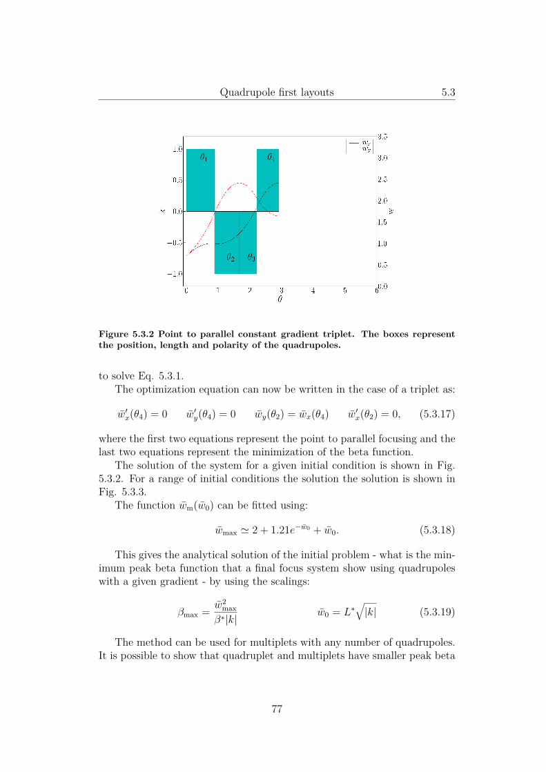
Quadrupole first layouts 5.3
Figure 5.3.2 Point to parallel constant gradient triplet. The boxes representthe position, length and polarity of the quadrupoles.
to solve Eq. 5.3.1.The optimization equation can now be written in the case of a triplet as:
w′x(θ4) = 0 w′y(θ4) = 0 wy(θ2) = wx(θ4) w′x(θ2) = 0, (5.3.17)
where the first two equations represent the point to parallel focusing and thelast two equations represent the minimization of the beta function.
The solution of the system for a given initial condition is shown in Fig.5.3.2. For a range of initial conditions the solution the solution is shown inFig. 5.3.3.
The function wm(w0) can be fitted using:
wmax ' 2 + 1.21e−w0 + w0. (5.3.18)
This gives the analytical solution of the initial problem - what is the min-imum peak beta function that a final focus system show using quadrupoleswith a given gradient - by using the scalings:
βmax = w2max
β∗|k|w0 = L∗
√|k| (5.3.19)
The method can be used for multiplets with any number of quadrupoles.It is possible to show that quadruplet and multiplets have smaller peak beta
77

Quadrupole first layouts 5.3
Figure 5.3.3 Solution for a triplet final focus system. The figure shows thenormalized lengths θi = li
√|k| and the maximum w =
√β as a function of the
initial conditions parameterized according to w0 = L∗√|k|.
functions with respect to the triplets, but they results in much longer struc-ture. The chromatic aberrations, on the contrary, do not depend on thenumber of quadrupoles in the multiplets. The triplets therefore represent afavorable solution.
5.3.6 Parameter spaceUsing Eq. (5.3.19 and 5.3.18, it is possible to plot the maximum beam sizeof the beam in the triplet as a function of the gradient using the simplifiedmodel. This function divides the plane in a region where the focusing systemsthat have a negative focal length (above the black line in Fig. 5.3.4) and theone having positive focal length.
It is possible to draw in the same plot the region of the aperture andgradient compatible with NbTi magnets (red region). A rough estimateimpose a the peak field of 8 T at the edge of the beam region diameter adefined by a = 33σ + 22 mm.
Figure 5.3.4 shows that if the gradient decrease the aperture requiredby the beam increases slower than the aperture compatible with a givenpeak field. It implies that the smaller is the gradient, the larger will be theaperture margins. The clear advantage of low gradient quadrupole magnetsis limited by the fact that the quadrupoles needs to be longer, the beta
78

Quadrupole first layouts 5.3
Figure 5.3.4 Triplet parameters space for the LHC upgrade. The intersectionof the three shaded regions contains all the possible apertures and gradientscompatible with a final focus system using NbTi quadrupoles. The blue regionrepresents the intrinsic focusing limitations of a triplet assemblu. The redregion represents the limitation of the NbTi technology that cannot hold peakfield in the coil larger than 8 T. The gray region represents the limitationsof the intrisic aberrattions (natural chromaticity and long range beam beaminteractions) of the final focus system.
79

Quadrupole first layouts 5.4
functions become larger and the chromatic aberrations increase. Anotherdisadvantage is that the number of long range interaction increases as well.For this reason Fig. 5.3.4 show another region (blue) delimited by a linewhich represent a rough estimation of the above mentioned limits.
The simplified model gives an indication of the parameters of possiblefocusing systems. However a realistic implementation is necessary to testthe hypothesis and identify further limitations.
5.4 Four flavors of quadrupole first layoutsFour layouts that span the parameter space and modularity for NbTi tech-nology are proposed and studied extensively in order identify and quantifythe merits and challenges.
A study has been performed to identify the possibilities for a replacementof the nominal triplet ( see [dM07a]). Four different layouts have been pro-posed (see [KRT07] and [BdMO07]) in order to explore the parameter spaceand identify the benefits and limitations of several design criteria.
Once the gradient is fixed, is necessary to introduce gaps between thequadrupoles in order to make room for coil ends that do not contribute tothe field and magnet interconnections. Additional room can be reserved forcorrector packages.
The optimal quadrupole lengths are in general different for every unit; onehas to trade the aperture margins and the overall lengths with the possibilityof using equal sized modules that reduce the cost of the equipment in termsof R&D and spare policy. It is worth noting that the nearest quadrupole tothe IP always requires a smaller aperture. Therefore it is possible to use astronger quadrupole with a smaller aperture and the same peak field withrespect to the other units resulting in a gain in the overall length and thebeta peak. Also in this case it is possible to trade this optimization with thecost of the equipment and the spare policy. In addition the larger aperturemargins of the first unit can be used to install thick shielding tubes thatprotects the coils from the debris coming from the collisions.
Four different layouts (see Fig. 5.4.5, 5.4.6, 5.4.7, 5.4.8) were designedand studied using different gradients and modularity options.
All data and analysis are collected in [dMT], only a selection is showedin the following parts.
Compact This option (see Fig. 5.4.5) uses a triplet layout and the lowestpossible gradient compatible with tolerable aberrations. The overalllength is minimized (the name comes from there) using an optimized
80

Quadrupole first layouts 5.4
Figure 5.4.5 Upgraded IR layout: “Compact”. The layout is optimized tofeature the largest aperture margin and be as compact as possible.
Figure 5.4.6 Upgraded IR layout: “Modular”. The layout is designed to havethe quadrupole modules of the same lengths.
81

Quadrupole first layouts 5.4
Figure 5.4.7 Upgraded IR layout: “Lowbetamax”. The layout is designed toreduce the peak beta function.
Figure 5.4.8 Upgraded IR layout: “Symmetric”. The layout is designed tohave the smallest peak beta function compatible with only two module lengths.[KRT07]) .
82

Quadrupole first layouts 5.5
gradient for Q1 and optimized lengths for Q1, Q2 and Q3. The gapbetween the quadrupoles is 1 m for the interconnection (a recent study[Par] established that the minimum distance between quadrupoles intwo different cryostats is 1.3 m but smaller in case they share thesame cryostats). In order to find a suitable collision optics an addi-tional Q6 module has been installed. This layout has been proposed in[BdMO07].
Modular This option (see Fig. 5.4.6,) uses a quadruplet design with anintermediate gradient. All the modules have the same length (the namecomes from there) but the first two have a larger gradient implyingeither a reduced aperture for the first two modules or reduced aperturemargins in the other modules. The gap between the quadrupoles is 1 m.An advantage of this option is the large set of gaps that can be usedfor mask absorbers or corrector magnets. In order to find a suitablecollision optics an additional Q6 module has been installed. This layouthas been proposed in [BdMO07].
Lowbetamax This option (see Fig. 5.4.7,) uses a triplet layout and thehighest gradient compatible with some additional aperture margin inthe triplet. The first element uses a reduced aperture and modulesof three different lengths. These choices limit the peak of the betafunction in the triplet (the name comes from there). No additionalquadrupole modules are installed. This layout has been proposed in[BdMO07].
Symmetric This option (see Fig. 5.4.7,) uses a triplet layout and the high-est gradient compatible with some additional aperture margin in thetriplet. This option uses only two different modules of different lengthbut same aperture and gradient. The modules are arranged almostsymmetrically with respect to the center of the triplet assembly (thename comes from there). The gaps are the same with respect to thenominal layout. This triplet layout first appeared in [KRT07].
These options do not cover all the possibilities and should be consid-ered working hypothesis for identifying merits and limitations for the severaloptions in terms of gradient and modularity.
The layout data is summarized in Table 5.1:For these layouts collision optics with crossing schemes for the entire LHC
have been developed. As an example see Fig. 5.4.9.
83

Quadrupole first layouts 5.5
Compact Modular Lowbetamax SymmetricL* [m] 23 23 24 23Gradient [T/m] 91,68 115,88,82,84 168,122 122Module L [m] 12.2,14.6,11 4.8 7.4,5.7,4.9 9.2,7.8Total L [m] 55 68 40 41LRBB 23 26 19 19Aper. MQX [mm] 170,220 130,170 90,130 130B.S. MQX [mm] 74,79;99,104 54,59;99,104 34,39;54,59 54,59B.S. D1 [mm] 50,64;45,64 50,64;45,64 50,64;45,64 50,64;45,64
Table 5.1 Layout parameters for different LHC interaction region layouts.Some layouts that require different gradients and modules lengths. The beamscreen apertures are given in term of half gap and radius and for the MQXthe two couples refer to the two apertures. The quadrupole apertures wereproposed in [BT] . The D1 apertures are proposed in [Far] .
Figure 5.4.9 Collision optics for Beam 1 in IR 5 for a quadrupole first layouts.
84
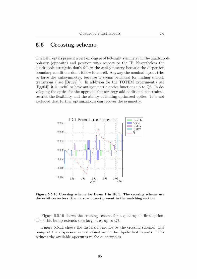
Quadrupole first layouts 5.6
5.5 Crossing scheme
The LHC optics present a certain degree of left-right symmetry in the quadrupolepolarity (opposite) and position with respect to the IP. Nevertheless thequadrupole strengths don’t follow the antisymmetry because the dispersionboundary conditions don’t follow it as well. Anyway the nominal layout triesto force the antisymmetry, because it seems beneficial for finding smoothtransitions ( see [Bru99] ). In addition for the TOTEM experiment ( see[Egg04]) it is useful to have antisymmetric optics functions up to Q6. In de-veloping the optics for the upgrade, this strategy add additional constraints,restrict the flexibility and the ability of finding optimized optics. It is notexcluded that further optimizations can recover the symmetry.
Figure 5.5.10 Crossing scheme for Beam 1 in IR 1. The crossing scheme usethe orbit correctors (the narrow boxes) present in the matching section.
Figure 5.5.10 shows the crossing scheme for a quadrupole first option.The orbit bump extends to a large area up to Q7.
Figure 5.5.11 shows the dispersion induce by the crossing scheme. Thebump of the dispersion is not closed as in the dipole first layouts. Thisreduces the available apertures in the quadrupoles.
85

Quadrupole first layouts 5.7
Figure 5.5.11 Parasitic dispersion Beam 1 in IR 1. The parasitic dispersiongenerated by the crossing scheme.
5.6 Mechanical aperture
The quantity n1 (which gives the required distance in sigma of the primarycollimator, see [BCL+04] and Sec. 3.4.1) has been used for evaluating theaperture margins in the interaction region. The aperture model is indicatedfor the new elements in Table 5.1. For the rest of the elements the aperturemodel is the same as the one of the official LHC optics with few exceptionsfor D2 Q4 and Q5. The aperture of these elements has been optimized forthe injection optics with a particular orientation of the beam screen. Incase of the upgraded optics the beta functions and as a consequence thecrossing scheme pose tighter constraints at collision. The beam screens areconsequently rotated in the locations where it is possible to increase aperturemargins.
The apertures are computed using closed orbit tolerances of 3 mm, en-ergy spread of δ = 0.00086 and nominal aperture tolerances. Additionalinformations are given in [Far07].
The results are summarized in Tab. 5.2 from which it is possible to seethat the lower gradient options (Compact and Modular), while offering largeaperture margins in the triplet, show aperture bottlenecks in the matchingsection. The higher gradient options (Lowbetamx and Symmetric), on thecontrary, offer a better balance of the aperture margins.
86

Quadrupole first layouts 5.7
Compact Modular Lowbetamax Symmetric LHCMQX, ap 1 20.026 14.141 7.821 15.466 7.215MQX, ap 2 16.953 12.633 8.830 8.438 6.845D1 5.303 6.379 7.607 7.323 7.431D2 5.372 4.271 7.959 6.518 15.152Q4 7.387 6.432 8.685 7.184 15.615Q5 4.701 3.859 10.425 7.028 16.871
Table 5.2 Aperture bottlenecks for the upgrade optics and the nominal LHCin terms of n1
Figure 5.6.12 Aperture for Beam 1 in IR 1 in terms of n1.
87

Quadrupole first layouts 5.8
Figure 5.6.13 Aperture for Beam 1 in IR 1 in terms of n1 with the beam screenrotated starting from D2. It is possible to note the gain of a aperture marginwith respect the non rotated option showed in Fig. 5.6.12.
5.7 ChromaticityThe upgrade optics present stronger chromatic effects with respect to thenominal layout due the reduction of β∗ which implies a stronger impact ofquadrupole errors in the final focusing system.
Table 5.3 shows the values for the required strengths of the arc sextupolesfor compensating the first order chromaticity and the off momentum betabeating for two different energy errors.
The results show that, while the natural chromaticity is still correctableby the arc sextupoles, the off momentum beta beat increases by a factor of3 to 5 with respect to the nominal values. It is not clear whether the rest ofthe LHC subsystems can cope with such a large beating or if this effect canbe corrected while keeping acceptable flexibility in the machine.
5.8 Dynamic apertureIn collision the dynamics aperture (DA) is dominated by the non linear fieldsin the interaction region. The larger contribution to the reduction of DA isthe “other” beam which should reduce the DA to 6σ.
Another important contribution comes from the field imperfections in
88

Quadrupole first layouts 5.8
Figure 5.7.14 Chromatic change of the tune for a quadrupole first layout. Thenon linear terms are much stronger with respect to the nominal values.
Figure 5.7.15 Chromatic beta-beating at δ = 3 · 10−4 for a quadrupole firstlayout. The beta-beating is three times larger with respect to the nominalvalues.
89

Quadrupole first layouts 5.9
Compact Modular Lowbetamax Symmetric LHCSextupoles [%] 88,56 87,58 74,46 75,46 48,28Beat. δ = 3 · 10−4 [%] 40 40 30 30 10Beat. δ = 8 · 10−4 [%] 150 150 100 105 30
Table 5.3 Chromatic aberrations for the upgrade optics and the nominal LHC.The first row show the required strength of the arc sextupoles for compensatingthe first order chromaticity, while the last two rows present the off momentumbeta beating for two different energy error.
Compact Modular Lowbetamax Symmetric LHCFull 16 11 14 12 12Triplet only 22 17 14 12Triplet excluded 16 11 20 16
Table 5.4 Minimum DA over 60 seeds without beam beam effect and fieldimperfections of D1 and D2. The second row and the third row show theDA excluding in addition all field imperfections but the triplet and the tripletrespectively. The field quality for the triplets is estimated using the resultsshowed in [KRT07].
large beta area (i.e. triplets, D1, D2 and the first elements of the matchingsection). For the LHC it has been estimated that for preserving the DA to 6σincluding beam beam, the minimum DA over 60 seeds without beam beameffect should be larger than 12σ (see [BCL+04]).
In case of the upgrade it is important to design magnets with a fieldquality that preserve a DA of 12σ. Estimates for the field quality of newmagnets can be found using the scaling laws presented in [KRT07] and theexisting production for the LHC.
Table 5.4 shows the results of the DA studies for the four upgrade opticsand the LHC.
Designs with larger aperture margins present larger DA when only tripletserror are included. In case of aperture bottlenecks in the matching section,the field quality of those elements starts to be the dominant one. These twofacts explain the large differences between the Compact and Modular designwith respect to the Lowbetamax and Symmetric. The differences betweenthe Symmetric and Lowbetamax, very similar in terms of field quality, couldbe explained by the averaging effect of a different number of modules andthe uncertainty of the method.
90

Quadrupole first layouts 5.10
5.9 Transition to injectionAn optics with β∗ > 5 m is required at injection because the transverseemittance is four time larger. A set of transition optics should be found inorder change the IR configuration from injection to collision. The quadrupolesettings should smoothly change in order to accommodate the restrictions inthe power supplies. The transition optics should also have the same phaseadvance in order keep the tune of machine stable.
For the LHC the set of transition optics is hard to find because of the limi-tations in the maximum current of the magnets and limitations of mechanicalaperture in the LSS. Without one of these two limitations is very straight-forward to find a solution because the number of parameters are larger thanthe number of constraints. The parameters are not truly independent andthe solution may or may not exist in case of limitations of aperture, whichtranslates in limitations of the maximum beta in some location, and limi-tations of quadrupole strengths, which translate in limitations of tunability(roughly proportional to the product βk).
A preliminary study shows that is possible to keep the phase advance ofthe insertion for a large range of β∗ only for Lowbetamax and Symmetric.
5.10 ConclusionThe development of four different optics showed the actual limitations andchallenges for quadrupole first layouts.
The results presented so far show that the Lowbetamax option show thebest overall performance closely followed by the Symmetric option whichoffers a simpler tough less flexible design. Both options can be further opti-mized to gain aperture margins and represent a good starting point for thefinal design.
The studies pointed to outstanding issues that need to be further inves-tigated.
Aperture bottleneck have been identified in D1, D2, Q4, Q5. The lim-itation in D1 is avoidable and requires a new design for the dipole. Thelimitations for D2, Q4, Q5 depend on the triplet layout. A further opti-mization can reduce the problem but on one hand the triplets have a limitednumber of free parameters to use and on the other hand the LSS is notflexible enough to accept all possible optics function that merely fulfill theaperture requirements. This limitation is more severe for the Compact andModular options, while is presumably fixable for the Symmetric option andbarely acceptable for the Lowbetamax option.
91

Quadrupole first layouts 5.10
The impact of the larger off momentum beta beat and the third orderchromaticity need to studied. It is a global quantity and it may affect otherLHC subsystem (e.g the collimation system).
The presented solution even though were designed to be as realistic aspossible, represents an effort to study the possibilities and implication ofseveral design criteria: gradient and aperture of the quadrupoles, number ofmodules, triplet or quadruplet design.
The analysis presented is not exhaustive. For a more realistic designmany refinements are need. In particular it is important to check whether theheat load and radiation damage levels are compatible with the new elementsand redesign the final focus system for increasing the aperture margins andreserving the right locations for correctors and diagnostics (orbit correctorand BPM).
92

Chapter 6
Conclusions
An upgrade of the LHC interaction regions allows to increase the luminosityby a factor of 1.6 (up to 2) with respect to the nominal performance. Theupgrade of the IR affects a limited part of the LHC and it has fewer sideaffects with respect to other means of increasing the luminosity (e.g. bunchintensity and number of bunches).
The upgrade of the LHC interaction region aims at a reduction of beamtransverse size at the IP by reducing β∗ from 55 cm to 25 cm. The presentIR cannot reach β∗ = 25 cm because the focus system close to the IP (i.e.triplet) has limitations in the mechanical aperture of the quadrupoles magnet.In addition the present layout is designed to be protected from the debriscoming from the IP only for the ultimate luminosity, therefore an upgrade ofthe luminosity will certainly require a redesign of the particle absorbers.
Being aware of those limitations, two design schemes are proposed andstudied, the dipole first layouts and the quadrupole first layouts, which ad-dress some of the limitation of the present layout.
The dipole first layouts modify the structure of the present layout and ex-change the position of the focusing system and the separation recombinationdipoles. The dipoles can act as absorbers because of the spectrometer effect.Their position reduces the number of parasitic interactions between the twobeams that is a source of reduction of beam lifetime. This advantages arecounterbalanced by the drawbacks of having the focusing system farther fromthe IP. It implies a growth of the beam size and beta function. The large betafunctions are a source of chromatic aberrations, sensitivity to magnet fieldimperfections and aperture bottlenecks in the matching section. In order tocope with these limitations, the layout studied in the thesis assume mag-net parameters at the edge of the theoretical limit of the Nb3Sn technology,currently under active development. Nevertheless the overall performance ofthe dipole first layout studied in the thesis proved that the implementation
93

Conclusions 6.0
is still challenging.Quadrupole first layouts represent instead a viable option for an upgrade.
A quadrupole first layout does not imply a change of the structure of theinteraction region, but an optimization of the focus system. It has beenassumed that the magnet should use NbTi magnets, the technology usedin the LHC that is proved feasible as of today in order to design optionsthat are practically realizable. In this case the challenge is to find optionswith better performance as compared to the nominal LHC using the sametechnology. The only difference is an increase of experience in manufacturingNbTi magnets, as compared to the one at the time the LHC was designed.The thesis shows the development of an analytical method that allows tofind the intrinsic limitations of a focusing system. Using this information,together with the limitations of the NbTi technology and the one comingfrom the beam dynamics, it is possible to define a region of parametersthat fulfill the requirements of the upgrade and are compatible with theexisting technology. The analytical method gives also indications on how toconstruct optimized layouts and it has been used to design and study realisticimplementations of quadrupole first layouts. In particular it was possible todemonstrate that longer and weaker quadrupoles allow a reduction of thetransverse beam size at the IP and at the same time an increase of theaperture margins.
The implementations address several design criteria such as large aperturemargins for extending the flexibility and reducing the energy deposited in themagnet coils, modular design to reduce the number of spares magnet andtherefore the overall cost of the upgrade and finally reducing the intrinsicaberrations and avoid aperture bottlenecks in the matching section. Theanalysis showed that some of the options require additional changes in thematching section, while others reach the upgrade goals by changing a limitednumber of quadrupoles.
These results contributed to the approval of a CERN project that aims atbringing the LHC to ultimate performance by implementing a low gradientquadrupole first layout.
94

Appendix A
Optimization tools foraccelerator optics
A.1 IntroductionA new matching algorithm and a new matching mode have been developedand implemented for MadX [SIG]. The new algorithm, called JACOBIAN,is able to solve a generalized matching problem with an arbitrary number ofvariables and constraints. It aims at solving the corresponding least squareproblem. The new mode, called USE_MACRO, allows the user to con-struct his own macros and expressions for the definition of the constraintsin a matching problem. The new algorithm combined with the macro con-structs was successfully used for finding optic transitions and a non-linearchromaticity correction. This new approach can be seen as a major upgradeof the matching capabilities of MadX taking advantage of various moduleslike TWISS, PTC,TRACK, SURVEY, APERTURE, and so on.
MadX provides several other matching algorithms:
• LMDIF: fast but limited to problems where the number of variables isnot greater than the number of constraints and the constraints aredifferentiable,
• SIMPLEX: suited for problems where the constraints are differentiable,slower then LMDIF, not always suited for constrained problems forwhich solutions tend to go far from the starting point;
The new matching routines JACOBIAN has been developed in order toprovide solutions for:
• problems for an arbitrary number of variables and constraints,
95

Optimization tools for accelerator optics A.2
• constrained problems where it is interesting to find the closest solutionfrom the starting point,
• constraints on the variation of a variable (see SLOPE option in VARYcommand [SIG]);
MadX can match quantities calculated by the twiss command and storedin the TWISS or SUMM table. A new mode USE_MACRO has been developedto let the user define its own observables using all available MadX modules.
A.2 Optimization and least-sqaure fittingAn optimization problem can be written as:
f(x) A function Rn : R to be minimized
ci(x) = 0, i ∈ E A set of equalities to be fulfiled
ci(x) ≥ 0, i ∈ I A set of inequalities to be fulfiled
The function f can be expanded in Taylor series, therefore
f(x+ p) = f(x) +∇f(x+ tp)Tp t ∈ [0, 1] (A.2.1)
f(x+ p) = f(x) +∇f(x)Tp+ 12p
T∇2f(x+ tp)p t ∈ [0, 1]. (A.2.2)
x∗ is local minimizer if
∇f(x∗) = 0 ∇2f(x∗)positive semidefinite (A.2.3)
A set S is convex if for every x, y ∈ S, αx+(1−α)y ∈ S for all α ∈ [0, 1].A function f is convex if for every x, y ∈ S, f(αx+(1−α)y) ≤ αf(x)+ (1−α)f(y) for all αin[0, 1].
If a function is convex a local minimizer is also a global minimizer.A least square problem is defined if f is
f(x) = 12∑
ri(x)2 = 12 |r(x)| (A.2.4)
If J(x) = ∂ri∂xj
is the Jacobian then
∇f(x) = J(x)T r(x) ∇2f(x) = J(x)TJ(x) + r(x)T∇2r(x) (A.2.5)
96

Optimization tools for accelerator optics A.3
If r(x) are linear
x∗ =∑σi 6=0
uTi r
σivi +
∑σi=0
τivi (A.2.6)
If τi = 0 then x∗ is the solution which minimizes |x∗|.
A.3 Singular value decompositionA m× n rectangular matrix M can always be decomposed in
M = UΣV ∗ (A.3.1)
where U is a m×m matrix, Σ is a m× n diagonal matrix and V is a n× nmatrix.
IfM is a linear transformation a M−→ b the following commutative diagramapplies:
aM−−−→ byV yU
αΣ−−−→ β
(A.3.2)
If vi is the ith column of V , σi is the ith element of the Σ diagonal andui the ith column of U then
b =∑i
uiσiv∗i a (A.3.3)
or
Mvi = σiui (A.3.4)
The pseudo inverse of M can be calculated by:
M−1 = V Σ+U∗ (A.3.5)
M−1ij =
min(n,m)∑t=1
Vit1SttUtj, (A.3.6)
where Σ+ is Σ∗ with nonzero entries replaced by their reciprocal.If the singular values are sorted in crescent order and s is the index of
the last non-zero singular value then:
97

Optimization tools for accelerator optics A.4
• u1, . . . , us span the range of M−1
• us+1, . . . , um span the null space of M−1
• v1, . . . , vs span the range of M
• vs+1, . . . , vn span the null space of M
A.4 JACOBIAN algorithm
AlgorithmThe algorithm is based on the Newton-Raphson method.
A matching problem can be defined as
c = f(v)
where c is the vector of the c constraints, v is the vector of the v variablesand f is vector field representing accelerator quantities.
If c0 = f(v0) is a solution for c0 close to c then
c = c0 + DfDv (v0)δv +O
(|δv|2
)and the solution can be found by iterating the equations:
v = v0 + αnδvDfDv = J δv = J−1(c− c0).
where J is the Jacobian of the transformation, δv is the vector whichpoints to the solution, αn is the succession 2−n and n is chosen such thatthe penalty function |c− c0| is smaller than the one of the previous step (seeBISEC in [SIG]).
If J is a c× v matrix and c = v, the system can be solved exactly,if v > c or v < c is solved by a QR or LQ decomposition [ABB+99] yieldingthe minimization of |c− c0| or |δv| respectively.
If a constraint is an inequality:
• it’s removed from the system when it is fulfilled,
• otherwise it is treated as an equality.
At each iteration step, if a variable it is assigned out of its boundaries:
98

Optimization tools for accelerator optics A.4
• if v > c the variable is excluded from the set and linear system is solvedagain,
• if v = c or there were too many exclusions the variable is reseted to itslimit (see STRATEGY in [SIG]).
In addition, before the matching process, the following transformationcan be applied to variable vector:
• a uniform random vector is added to the variables (see RANDOM in [SIG])in order to avoid local minima;
• the variables are moved towards a desired value (see COOL, BALANCE,OPT in [SIG]) in order to force the final solution.
Figure 1 shows the scheme of the algorithm.
USE_MACROThe new mode is based on the idea that:
• the constraints can be user defined expressions,
• the calculations for evaluating these expressions can be defined viamacros.
In this way, every quantity which can be calculated via macros and ex-pressions can be accessed by the user and be used by the matching algorithm.
The expressions can contain algebraic functions of values from the MadXtables through the TABLE construct.
The syntax is slightly different from the old style matching and has 2variants:
• using an already defined macro
m1: macro= {y=(x-3.5)*(x+2)*(x-4); };match,use_macro;
vary,name=x;use_macro: name= m1;constraint,expr= y=0;jacobian,tolerance=1.e-24;
endmatch;
99
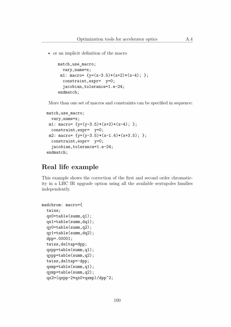
Optimization tools for accelerator optics A.4
• or an implicit definition of the macro
match,use_macro;vary,name=x;
m1: macro= {y=(x-3.5)*(x+2)*(x-4); };constraint,expr= y=0;jacobian,tolerance=1.e-24;
endmatch;
More than one set of macros and constraints can be specified in sequence:
match,use_macro;vary,name=x;
m1: macro= {y=(y-3.5)*(x+2)*(x-4); };constraint,expr= y=0;
m2: macro= {y=(y-3.5)*(x-1.4)*(x+3.5); };constraint,expr= y=0;jacobian,tolerance=1.e-24;
endmatch;
Real life exampleThis example shows the correction of the first and second order chromatic-ity in a LHC IR upgrade option using all the available sextupoles familiesindependently.
madchrom: macro={twiss;qx0=table(summ,q1);qx1=table(summ,dq1);qy0=table(summ,q2);qy1=table(summ,dq2);dpp=.00001;twiss,deltap=dpp;qxpp=table(summ,q1);qypp=table(summ,q2);twiss,deltap=-dpp;qxmp=table(summ,q1);qymp=table(summ,q2);qx2=(qxpp-2*qx0+qxmp)/dpp^2;
100

Optimization tools for accelerator optics A.5
qy2=(qypp-2*qy0+qymp)/dpp^2;};
use,sequence=lhcb1;match,use_macro;vary, name=ksd1.a12b1; vary, name=ksd1.a23b1;vary, name=ksd1.a34b1; vary, name=ksd1.a45b1;vary, name=ksd1.a56b1; vary, name=ksd1.a67b1;vary, name=ksd1.a78b1; vary, name=ksd1.a81b1;vary, name=ksd2.a12b1; vary, name=ksd2.a23b1;vary, name=ksd2.a34b1; vary, name=ksd2.a45b1;vary, name=ksd2.a56b1; vary, name=ksd2.a67b1;vary, name=ksd2.a78b1; vary, name=ksd2.a81b1;vary, name=ksf1.a12b1; vary, name=ksf1.a23b1;vary, name=ksf1.a34b1; vary, name=ksf1.a45b1;vary, name=ksf1.a56b1; vary, name=ksf1.a67b1;vary, name=ksf1.a78b1; vary, name=ksf1.a81b1;vary, name=ksf2.a12b1; vary, name=ksf2.a23b1;vary, name=ksf2.a34b1; vary, name=ksf2.a45b1;vary, name=ksf2.a56b1; vary, name=ksf2.a67b1;vary, name=ksf2.a78b1; vary, name=ksf2.a81b1;use_macro,name=madchrom;constraint,expr= qx1=2;constraint,expr= qy1=2;constraint,expr= abs(qx2)<2;constraint,expr= abs(qy2)<2;jacobian,calls=10,bisec=3;endmatch;
This problem is solved by JACOBIAN in 5 iteration for a total of 160 callsof the macro. The problem could also be solved by the SIMPLEX methodbut solution doesn’t converge. Reducing the number of variables to 4 inorder to use LMDIF brings to a solution which requires 50% more strength forthe sextupoles because JACOBIAN, via the LQ decomposition, solve the leastsquare problems in the iterations.
A.5 ConclusionThe JACOBIAN procedure combined with the USE_MACRO construct has beensuccessfully used for finding smooth optics transitions, estimation of the
101

Optimization tools for accelerator optics A.5
tunability of insertion regions ([SSdMF06]) and for non-linear chromaticitycorrection([dMBR06],[dMB06]).
JACOBIAN performs better than the other methods in case that
• the problem is almost linear and the constraints are differentiable;
• the starting point is close to the solution;
• the problem is such that v > c;
otherwise SIMPLEX or LMDIF provide better results, for problems in whichthe constraints are not differentiable or differentiable respectively.
USE_MACRO extends the optimization capabilities for linear and non-linearoptics, aperture, tracking, resonant driving terms and so on.
102

Optimization tools for accelerator optics A.5
start
apply COOLinit and RANDOM
reset values out of boundaries
compute penalty
end
main loop
repeat
input errors or converged
reset variables out of boundaries
compute penalty
not converged
converged
calculate jacobian
reset solution vector
print jacobian
STRATEGY=2
cut ineffective constraints
invert jacobian
update the starting point
error STRATEGY=1
cut variables
variables out of boudaries
and STRATEGY=3
yes
no
restore cuts
jacobian overdetermined or
too many cuts
Figure A.4.1 Algorithm of JACOBIAN
103

Optimization tools for accelerator optics
104

Bibliography
[ABB+99] E. Anderson, Z. Bai, C. Bischof, S. Blackford, J. Demmeladn J. Dongarra, J. Du Croz, A. Greenbaum, S. Hammarling,A. McKenney, and D. Sorensen. LAPACK Users’ Guide ThirdEdition. 1999.
[BC07] O. Bruening and P. Collier. Building a behemoth. Nature, 448,jul 2007.
[BCG+02] Oliver Sim Bruening, Roberto Cappi, R. Garoby, O. Groebner,W. Herr, T. Linnecar, R. Ostojic, K. Potter, L. Rossi, F. Rug-giero, Karlheinz Schindl, Graham Roger Stevenson, L. Tavian,T. Taylor, Emmanuel Tsesmelis, E. Weisse, and Frank Zim-mermann. LHC luminosity and energy upgrade : A feasibilitystudy. Technical Report LHC-Project-Report-626, CERN, De-cember 2002.
[BCL+04] O. Bruening, P. Collier, P. Lebrun, S. Myers, R. Ostojic,J. Poole, and P. Proudlock. LHC design report. TechnicalReport CERN-2004-003, CERN, 2004.
[BdM07] O. Bruening and R. de Maria. Low gradient triplet layout op-tions. In 3rd CARE-HHH-APD Workshop: Towards a Roadmapfor the Upgrade of the LHC and GSI Accelerator Complex LHC-LUMI-06, 2007.
[BdMO07] O. Bruening, R. de Maria, and R. Ostojic. Low gradient, largeaperture ir upgrade options for the lhc compatible with nb-timagnet technology. LHC-Report 1008, CERN, jun 2007.
[BFMG04] 0. Bruening, S. Fartoukh, and T. Risselada M. Giovannozzi. Dy-namic aperture studies for the lhc separation dipoles. TechnicalReport LHC-Project-Note-349., CERN, Geneva, Jun 2004.
105

Bibliography
[BKT07] B. Bellesia, J. Koutchouk, and E. Todesco. Field quality inlow-beta superconducting quadrupoles and impact on the beamdynamics for the large hadron collider upgrade. PRSTAB,10(062401):8, jan 2007.
[Bru99] O. Bruening. Optics solutions in ir1 and ir5 for ring-1 and ring-2of the lhc version 6.0. Technical Report CERN-LHC-Project-Note-187, CERN, April 1999.
[Bru05] O. Bruening. Possible dipole first options and challenges,September 2005. LHC LUMI 2005 CARE-HHH-APD Work-shop.
[BS84] Karl L. Brown and Roger V. Servranckx. First and secondorder charged particle optics. Technical Report SLAC-PUB-3381, SLAC, July 1984.
[BS87] Karl L. Brown and Roger V. Servranckx. Optics modules forcircular accelerator design. Nuclear Instruments and Methods inPhysics Research Section A: Accelerators, Spectrometers, Detec-tors and Associated Equipment, 258(3):480–502, August 1987.
[BT] F. Borgnolutti and E. Todesco. Quadrupole design forquadrupoles based on lhc nb-ti cables. Private comunication.
[Cha93] W. Chao. Physics of collective beam instabilities in high energyaccelerators. Wiley, New York, NY, 1993.
[CS58] E. D. Courant and H. S. Snyder. Theory of the alternating-gradient synchrotron. Annals of Physics, 1(3):1–48, jan 1958.
[CT99] A. Chao and M. Tigner. Handbook of accelerator physics andengineering. World Scientific, Singapore, 1999.
[CTZ07] R Calaga, R Tomás, and F Zimmermann. Crab cavity option forlhc ir upgrade. In 3rd CARE-HHH-APD Workshop: Towardsa Roadmap for the Upgrade of the LHC and GSI AcceleratorComplex, IFIC, Valencia, Spain, 16 - 20 Oct 2006, page 7 p,2007.
[dG97] E. T. d’Amico and G. Guignard. Analysis of a symmetric tripletand its application to ring insertions. CLIC-Note 341, CERN,May 1997.
106

Bibliography
[dG98] E.T. d’Amico and G. Guignard. Analysis of generic insertionsmade of two symmetric triplets. CERN-SL 98-014, CERN, May1998.
[dM05] R. de Maria. LHC IR upgrade: a dipole first option. In 2ndCARE-HHH-ADP Workshop on Scenarios for the LHC Lumi-nosity Upgrade LHC-LUMI-05, pages 33–39, September 2005.
[dM07a] R. de Maria. Layout design for final focus systems and applica-tions for the lhc interaction region upgrade. LHC-Report 1051,CERN, sep 2007.
[dM07b] R. de Maria. Lhc ir upgrade: Dipole first with chromaticityand dynamic aperture issues. In 3rd CARE-HHH-APD Work-shop: Towards a Roadmap for the Upgrade of the LHC and GSIAccelerator Complex LHC-LUMI-06, 2007.
[dMB06] R. de Maria and O. Bruening. A low gradient quadrupolefirst layout compatible with nbti magnet technology andbeta*= 0.25m. Technical Report CERN-LHC-Project-Report-933, CERN, June 2006. Presented at: European Particle Ac-celerator Conference EPAC’06 , Edinburgh, Scotland, UK , 26- 30 Jun 2006.
[dMBR06] R. de Maria, O. Bruening, and P. Raimondi. LHC IR upgrade:A dipole first option with local chromaticity correction. Tech-nical Report CERN-LHC-Project-Report-934, CERN, June2006. Presented at: European Particle Accelerator ConferenceEPAC’06 , Edinburgh, Scotland, UK , 26 - 30 Jun 2006.
[dMSS06] R. de Maria, F. Schmidt, and P. K. Skowronski. Advances inmatching with mad-x. In Proceedings of ICAP, September 2006.
[dMT] R. de Maria and R. Tomas. Web repository ofir upgrade options. http://care-hhh.web.cern.ch/CARE-HHH/SuperLHC_IRoptics/IRoptics.html.
[DZ07] U Dorda and F Zimmermann. Long-range beam-beam compen-sation with wires. In 3rd CARE-HHH-APD Workshop: Towardsa Roadmap for the Upgrade of the LHC and GSI AcceleratorComplex, IFIC, Valencia, Spain, 16 - 20 Oct 2006, page 3 p,2007.
107

Bibliography
[DZFS] U Dorda, F Zimmermann, W Fischer, and V Shiltsev. Lhcbeam-beam compensation using wires and electron lenses. InPAC07.
[Egg04] K. Eggert. Total cross-section, elastic scattering and diffractiondissociation at the large hadron collider at cern: Totem designreport. Cern-lhcc-2004-002, CERN, January 2004.
[Far] S. Fartoukh. Lss magnet aperture requirements. Presented atLIUWG in 27.09.2007.
[Far99] Stephane Fartoukh. Second order chromaticity correction ofLHC v6.0 at collision. Technical Report cern-lhc-project-report-308, CERN, October 1999.
[Far07] S. Fartoukh. Lss magnet aperture requirements for the lhcinsertion upgrade, a first estimate. Technical Report LHC-PROJECT-Report-1050, CERN, oct 2007.
[Far09] S. Fartoukh. Prospective for flat beam optics. Presented atLHC MAC 15-17 June 2009, 2009.
[FGdMG07] A. Faus-Golfe, R. de Maria, and R. Tomas Garcia. Limits onchromaticity correction. In 3rd CARE-HHH-APD Workshop:Towards a Roadmap for the Upgrade of the LHC and GSI Ac-celerator Complex LHC-LUMI-06, 2007.
[GAG+05] R. C. Gupta, M. Anerella, A. Ghosh, M. Harrison, J. Schmalzle,P. Wanderer, and N. V. Mokhov. Optimization of open mid-plane dipole design for LHC IR upgrade. Particle AcceleratorConference (PAC 05), May 2005.
[Gia99] F. Gianotti. Collider physics: Lhc. Atlas note 2000-001, CERN,sep 1999.
[GMV02] F. Gianotti, M. L. Mangano, and T. Virdee. Physics poten-tial and experimental challenges of the lhc luminosity upgrade.CERN-TH CERN-TH-2002-078, CERN, apr 2002.
[HM03] W. Herr and B. Muratori. Concept of luminosity. In CAS -Intermediate Course on Accelerator Physics, DESY, Zeuthen,Germany, 15 - 26 Sep 2003, 2003.
108

Bibliography
[JO97] J. B. Jeanneret and R. Ostojic. Geometrical acceptance in LHCversion 5.0. CERN-LHC-Project-Note 111, CERN, September1997.
[KAM+07] J-P. Koutchouk, R. Assmann, E. Métral, E. Todesco, F. Zim-mermann, R. de Maria, and G. Sterbini. A concept for thelhc luminosity upgrade based on strong beta* reduction com-bined with a minimized geometrical luminosity loss factor. InProceedings of PAC07, Albuquerque, New Mexico, USA, 2007.
[KRT07] J. P. Koutchouk, L. Rossi, and E. Todesco. A solution for phase-one upgrade of the LHC low-beta quadrupoles based on nb-ti.lhc-project-report 1000, CERN, April 2007.
[Mok05] Nikolai Mokhov. Energy deposition in midplane dipole. InLARP Collaboration Meeting 4, April 2005. Talk.
[Ohm05] K Ohmi. Study of crab cavity option for lhc. In 1st CARE-HHH-APD Workshop on Beam Dynamics in Future Hadron Collid-ers and Rapidly Cycling High-Intensity Synchrotrons, CERN,Geneva, Switzerland, 8 - 11 Nov 2004, 2005.
[Par] V. Parma. Space constraints for the triplet cryostats. Presentedat LIUWG in 18.10.2007.
[Peg84] S. Peggs. Minimising chromaticity in interaction regions withlong weak quadrupoles. In SSC Summer Study, 1984.
[Reg67a] E. Regenstreif. Phase-space transformations by means ofquadrupole multiplets. CERN 67-6, CERN, March 1967.
[Reg67b] E. Regenstreif. Possible and impossible phase-space transfor-mations by means of alternating-gradient doublets and triplets.CERN 67-8, CERN, March 1967.
[RS01] P. Raimondi and Andrei Seryi. Novel final focus design forfuture linear colliders. Phys. Rev. Lett., 86(17):3779 – 3782, apr2001.
[SIG] F. Schmidt, G. Iselin, and H. Grote. Madx manual.http://cern.ch/mad/.
[SJM+06] T Sen, J Jstone, Nikolai Mokhov, W Fischer, Ramesh Gupta,and Ji Qiang. Us-larp progress on lhc ir upgrades. In 2nd
109

Bibliography
CARE-HHH-APD Workshop on Scenarios for the LHC Lumi-nosity Upgrade, Arcidosso, Italy, 31 Aug - 3 Sep 2005, 2006.
[SJRT07] T Sen, J Jstone, V Ranjibar, and R Tomas. Ir upgrade withquadrupoles first and dipoles first. In 3rd CARE-HHH-APDWorkshop: Towards a Roadmap for the Upgrade of the LHCand GSI Accelerator Complex, IFIC, Valencia, Spain, 16 - 20Oct 2006, page 6 p, 2007.
[SSdMF06] P. K. Skowronski, F. Schmidt, R. de Maria, and E. Forest. Newdevelopments of mad-x using ptc. In Proceedings of ICAP 2006,September 2006.
[SSM05] T Sen, J Strait, and N Mokhov. Overview of possible lhc ir up-grade layouts. In 1st CARE-HHH-APD Workshop on Beam Dy-namics in Future Hadron Colliders and Rapidly Cycling High-Intensity Synchrotrons, CERN, Geneva, Switzerland, 8 - 11Nov 2004, 2005.
[TdMZ07] R. Tomas, R. de Maria, and F. Zimmermann. Crab cavity iroptics design with t=8mrad. In 3rd CARE-HHH-APD Work-shop: Towards a Roadmap for the Upgrade of the LHC and GSIAccelerator Complex LHC-LUMI-06, 2007.
[Tüc07] J Tückmantel. Technological aspects of crab cavities. In 3rdCARE-HHH-APD Workshop: Towards a Roadmap for the Up-grade of the LHC and GSI Accelerator Complex, IFIC, Valen-cia, Spain, 16 - 20 Oct 2006, page 6 p, 2007.
[Zie95] Volker Ziemann. Crude scaling laws for the dynamic aperture ofLHC from random non-linear errors. Technical Report CERN-SL-Note-95-20-AP, CERN, February 1995.
[Zim05] F Zimmermann. Beam-beam compensation schemes. In1st CARE-HHH-APD Workshop on Beam Dynamics in Fu-ture Hadron Colliders and Rapidly Cycling High-Intensity Syn-chrotrons, CERN, Geneva, Switzerland, 8 - 11 Nov 2004, 2005.Fulltext not available.
[Zim08] F. Zimmermann. Cern task force on lhc luminosity and en-ergy upgrade, organized by francesco ruggiero, 1st meeting03.07.2001, 2008. private comunication.
110

Bibliography
[ZK06] A V Zlobin and V Kashikhin. Study of 2-in-1 large-aperturenb3sn ir quadrupoles for the lhc luminosity upgrade. InEPAC06, page 3 p, 2006.
111

Bibliography
112

Curriculum VitaeRiccardo de Maria
Personal Data
First name Riccardo
Family name de Maria
Address Brookehaven National LaboratoryBldg 902A, 11973, Upton, NY, USA.
Telephones +41 328 746 1346 (Mobile)
E-Mail [email protected]
Place and Date of Birth Rome, Italy, December 19, 1977
Nationality Italian
Compulsory Military Service Done
Education
2008 PhD at the Ecole Polytechnique federales in Lausanne.Thesis: “LHC Interaction Region Upgrade”.
2004 “Laurea” degree (five years master course), in ElectricalEngineering at “La Sapienza” University of Rome, Italy.Thesis at CERN: “Time Transient Effects in Superconduct-ing Magnets”. Grade: summa cum laude.
2003 “JUAS Accelerator Physics and Accelerator TechnologiesDiploma”,Archamps, France. Grade and ranking respec-tively: A, 3rd/16; A, 1st/20.
1996 High School Degree “Maturita Scientifica”, at “Liceo Scien-tifico Statale Nomentano”, Rome, Italy. Grade: 54/60.
Work Experiences
2008-Today “Toohig” distinguished fellowship at Brookhaven NationalLaboratory, Upton, NY. Supervisor Dr. Steve Peggs.
2005-2008 Doctoral Student at CERN, Accelerator and Beam Depart-ment, in accelerator beam optics. Subject: “LHC Luminos-ity Upgrade”. Supervisor: Dr. Oliver Bruning.
2004 Technical Student at CERN, Accelerator Technologies De-partment, in numerical field computation. Laurea DegreeThesis : “Transient Time Effects in Superconducting Mag-nets”. Supervisor: Dr. Stephan Russenschuck.
1998–2000 Fellowship at “Dipartimento di Energetica”, “La Sapienza”University of Rome, during which I make assistance in us-ing didactic software, development and presentation ofphysics didactic experiences.Supervisor: Prof. Luigi Palumbo.
1

Other Experiences
2001–2003 Student representative at “La Sapienza” University of Rome.
7/1999–10/2000 Compulsory military service.
Honors
2004 EPAC 2004 Grant as outstanding student at JUAS.
1998 and 1999 Fellowship at “Dipartimento di Energetica” at “La Sapienza”University of Rome, Italy.
Research Activities
Beam dynamics and beam optics ( [1], [2], [3], [4], [5],[6], [7], [8], [9], [10], [11], [12] )
Electromagnetic modeling of superconducting magnets ([13], [14] [15], [16] )
Computer codes for beam dynamics and beam optics ([17], [18] )
Vibration measurements and data acquisition ( [19] )
Optimization algorithms ( [18] )
Skills
Numerical computation programming in Fortran (90,77)C/C++, Python. High performance linear algebra routines(BLAS, LAPACK, MKL). Computer algebra and numericalsoftware (Mathematica, Matlab and similar).
Design tool for magnet design and particle dynamics.
Scientific instrumentation for electronics and electromag-netic fields (oscilloscope, network analyzer, digitizer), dataacquisition (LabView, custom development with GPIB, VXI11).
Generic programming also in Java, Perl, Bash. Develop-ment mainly in Unix environments.
Experience in electronic design, control systems and RFengineering.
Foreign Languages
Italian Mother Tongue.
English Fluent in writing and speaking.
French Good.
Rome, June 16, 2008
2

References
[1] R. de Maria. Layout design for final focus systems and applications for thelhc interaction region upgrade. LHC-Report 1051, CERN, sep 2007.
[2] O. Bruening, R. de Maria, and R. Ostojic. Low gradient, large apertureir upgrade options for the lhc compatible with nb-ti magnet technology.LHC-Report 1008, CERN, jun 2007.
[3] O. Bruening and R. de Maria. Low gradient triplet layout options. In 3rdCARE-HHH-APD Workshop: Towards a Roadmap for the Upgrade of the LHCand GSI Accelerator Complex LHC-LUMI-06, 2007.
[4] R. de Maria. Lhc ir upgrade: Dipole first with chromaticity and dynamicaperture issues. In 3rd CARE-HHH-APD Workshop: Towards a Roadmap forthe Upgrade of the LHC and GSI Accelerator Complex LHC-LUMI-06, 2007.
[5] R. Tomas, R. de Maria, F. Ruggiero, and F. Zimmermann. Lhc upgradeir optics web repository. In 3rd CARE-HHH-APD Workshop: Towards aRoadmap for the Upgrade of the LHC and GSI Accelerator Complex LHC-LUMI-06, 2007.
[6] R. Tomas, R. de Maria, and F. Zimmermann. Crab cavity ir optics designwith t=8mrad. In 3rd CARE-HHH-APD Workshop: Towards a Roadmap forthe Upgrade of the LHC and GSI Accelerator Complex LHC-LUMI-06, 2007.
[7] J-P. Koutchouk, R. Assmann, E. Metral, E. Todesco, F. Zimmermann,R. de Maria, and G. Sterbini. A concept for the lhc luminosity upgradebased on strong beta* reduction combined with a minimized geometricalluminosity loss factor. In Proceedings of PAC07, Albuquerque, New Mexico,USA, 2007.
[8] A. Faus-Golfe, R. de Maria, and R. Tomas Garcia. Limits on chromaticitycorrection. In 3rd CARE-HHH-APD Workshop: Towards a Roadmap for theUpgrade of the LHC and GSI Accelerator Complex LHC-LUMI-06, 2007.
[9] R. de Maria and O. Bruening. A low gradient quadrupole first layout com-patible with nbti magnet technology and beta*= 0.25m. Technical ReportCERN-LHC-Project-Report-933, CERN, June 2006. Presented at: Euro-pean Particle Accelerator Conference EPAC’06 , Edinburgh, Scotland, UK ,26 - 30 Jun 2006.
[10] R. de Maria, O. Bruening, and P. Raimondi. LHC IR upgrade: A dipole firstoption with local chromaticity correction. Technical Report CERN-LHC-Project-Report-934, CERN, June 2006. Presented at: European ParticleAccelerator Conference EPAC’06 , Edinburgh, Scotland, UK , 26 - 30 Jun2006.
[11] M. Giovannozzi, R. de Maria, S. Fartoukh, S. Gilardoni, J.-B. Jeanneret,A. Lombardi, Y. Papaphilippou, and T. Risselada. Dynamical aperturestudies for the cern lhc: Comparison between statistical assignment ofmagnetic field errors and actual measured field errors. In Proceedings ofEPAC 2006, Edinburgh, Scotland, 2006.
3

[12] R. de Maria. A general method for final focus system design for circularcolliders. In print on Phys Rev ST Accel and Beams.
[13] B. Auchmann, R. de Maria, S. Russenschuck, and S. Kurz. 2d electromag-netic model of fast-ramping superconducting magnets. In Proceedings ofICAP 2006, Chamonix, France, 2006.
[14] B. Auchmann, R. de Maria, and S. Russenschuck. Comparative study ofinter-strand coupling current models for accelerator magnets. TechnicalReport CERN-AT-2006-11, CERN, June 2006. Presented at: European Par-ticle Accelerator Conference EPAC’06 , Edinburgh, Scotland, UK , 26 - 30Jun 2006.
[15] G. Moritz, J. Kaugerts, G. J. Escallier, G. Ganetis, A. K. Jain, A. Marone,J. F. Muratore, R. Thomas, P. Wanderer, B. Auchmann, R. de Maria,S. Russenschuck, and M. Wilson. Recent test results of the fast-pulsed 4 tcos dipole gsi 001. In Particle Accelerator Conference PAC 2005 , Knoxville,TN, USA , 16 - 20 May 2005, page 683, May 2005.
[16] R. de Maria. Time transient effects in superconducting magnets. MasterThesis for Universita degli Studi di Roma La Sapienza, jul 2004.
[17] P. K. Skowronski, F. Schmidt, R. de Maria, and E. Forest. New develop-ments of mad-x using ptc. In Proceedings of ICAP 2006, September 2006.
[18] R. de Maria, F. Schmidt, and P. K. Skowronski. Advances in matching withmad-x. In Proceedings of ICAP, September 2006.
[19] R. de Maria, T. Kroyer, and V.Shiltsev. Field fluctuation and beam screenvibration measurements in the lhc magnets. In Proceedings of PAC07, Al-buquerque, New Mexico, USA, 2007.
4