IEEE INTERNATIONAL CONFERENCE ON SHAPE MODELING AND APPLICATIONS (SMI) 2010 1

Ridge Extraction from Isosurfaces of Volumetric Data usingImplicit B-Splines

Suraj Musuvathy, Tobias Martin, Elaine CohenSchool of Computing, University of Utah

Abstract—Ridges are extremal curves of principal

curvatures on a surface that indicate salient intrinsic

features of its shape. This paper presents a novel

approach for extracting ridges of improved quality

from isosurfaces of volumetric scalar-valued grids by

converting them to implicit trivariate B-spline repre-

sentations. A robust tracing approach demonstrated

to extract ridges accurately from parametric B-

spline surfaces is extended to extract ridges directly

from the implicit representations resulting in accu-

rate and hence smoother, connected ridge curves as

compared to approaches that extract ridges directly

from discrete representations. This approach can

also be used to extract ridges directly from smooth

representations such as isosurfaces of volumetric B-

Spline CAD models and algebraic functions, and

extended to extract ridges from polygonal meshes,

as demonstrated in the paper. Most of the existing

approaches for ridge extraction address only crests,

a certain subset of the ridges on a surface. The

approach presented in this paper enables extraction

of all types of generic ridges on a surface thereby

presenting a complete solution.

Keywords—ridge; isosurface; volumetric grid;

polygonal mesh; implicit; B-Spline

1. INTRODUCTION

Ridges on a surface are shape intrinsic feature curves

that describe higher order differential properties of sur-

face geometry. Ridges are defined as loci of points where

one of the principal curvatures (κ1 ≥ κ2) attains a local

extremum along its principal direction (t1 or t21)[20],

[43].

φi = 〈∇κi, ti〉 = 0, i = 1 or 2 (1)

This paper refers to φi as the ridge function and to Equa-

tion (1) as the ridge equation. While other definitions

of ridge-like structures in the existing literature include

that of height ridges [15] and watershed ridges [36], we

address the extraction of principal curvature ridges in

this work. Crests, valleys, ravines are other frequently

used terms in the existing literature to describe extremal

curves of curvature. Ravines and valleys are ridges

of κ2. Crests are perceptually salient ridges where κ1

attains a local maximum along its principal direction

1t1 and t2 are 2D vectors representing the coefficients of the basisvectors of the tangent plane of the surface.

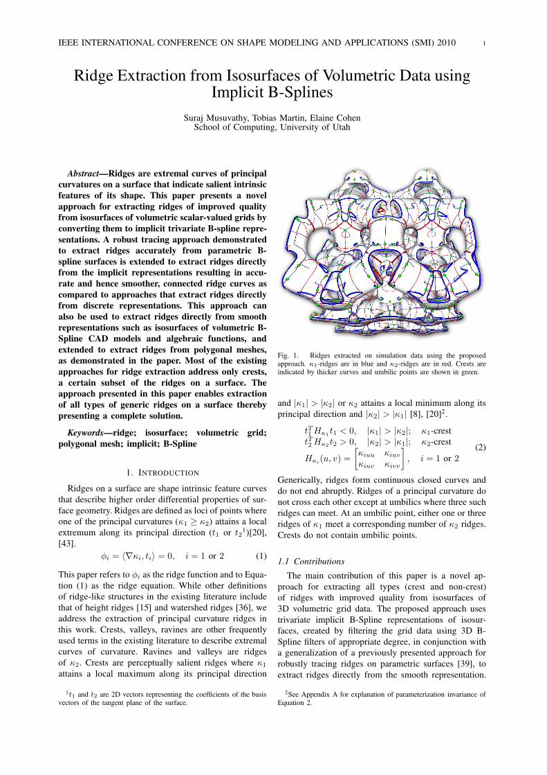
Fig. 1. Ridges extracted on simulation data using the proposedapproach. κ1-ridges are in blue and κ2-ridges are in red. Crests areindicated by thicker curves and umbilic points are shown in green.

and |κ1| > |κ2| or κ2 attains a local minimum along its

principal direction and |κ2| > |κ1| [8], [20]2.

tT1 Hκ1t1 < 0, |κ1| > |κ2|; κ1-crest

tT2 Hκ2t2 > 0, |κ2| > |κ1|; κ2-crest

Hκi(u, v) =

[

κiuu κiuv

κiuv κivv

]

, i = 1 or 2(2)

Generically, ridges form continuous closed curves and

do not end abruptly. Ridges of a principal curvature do

not cross each other except at umbilics where three such

ridges can meet. At an umbilic point, either one or three

ridges of κ1 meet a corresponding number of κ2 ridges.

Crests do not contain umbilic points.

1.1 Contributions

The main contribution of this paper is a novel ap-

proach for extracting all types (crest and non-crest)

of ridges with improved quality from isosurfaces of

3D volumetric grid data. The proposed approach uses

trivariate implicit B-Spline representations of isosur-

faces, created by filtering the grid data using 3D B-

Spline filters of appropriate degree, in conjunction with

a generalization of a previously presented approach for

robustly tracing ridges on parametric surfaces [39], to

extract ridges directly from the smooth representation.

2See Appendix A for explanation of parameterization invariance ofEquation 2.

3D data grids are abundantly available in the form of

medical images (MRI, CT scans), simulation data where

the resulting grids approximate solutions of discretized

partial differential equations and in the field of graphics

and visualization in the form of level set models [6]. The

proposed approach can also be used to extract ridges

directly from smooth implicit surface representations

such as those occurring from isogeometric analyses [23]

and implicit modeling systems [44]. Direct processing

of volumetric grid data avoids potentially difficult prob-

lems associated with extracting isosurfaces in the form

of discrete representations such as polygonal meshes.

Trivariate B-Splines have been previously used for ren-

dering [45] and filtering [34] of volumetric data and

implicit modeling [44]. Our proposed method comple-

ments this approach with a tool for extracting impor-

tant shape features directly from volumetric grids and

smooth implicit surface representations. In this paper,

the proposed approach is demonstrated to extract ridges

directly from medical image data, discrete simulation

data, isosurfaces of volumetric B-Splines occurring from

isogeometric analysis and algebraic functions. Further,

the method is extended to compute ridges from discrete

representations such as polygonal meshes by converting

them to trivariate B-Spline representations.

The consequence of tracing on a smooth representa-

tion is that the extracted ridge curves conform to generic

behavior and are therefore continuous connected curves.

B-Splines act as low pass filters on the data grid and

tends to smooth out high frequency characteristics such

as noise and thus the ridges do not have unexpected

undulations. In addition, a smooth representation allows

robust detection of isolated umbilics, and thus, ridges

around umbilics, to present a complete solution. Figure

1 shows ridges and crests extracted using our approach

from an isosurface of a 3D grid resulting from a simu-

lation. This isosurface has cylindrical regions with near

circular cross-sections that are non-generic. So ridges

can terminate abruptly as they get closer to such regions.

Other types of ridges including elliptic and hyperbolic

ridges are distinguished based on [39] as demonstrated

in Figure 6 (c).

1.2 Applications of Crest and Non-crest Type Ridges

Ridges have been used as landmarks for shape match-

ing and registration [19], [26], [42], [49], as indicators

of the quality of product designs [25], [22], as visual

cues for effective visualization [12], [24], [31] and

several other shape analysis tasks [29], [50]. Most of

the previous applications use crests mainly because there

are few methods for robust extraction of all types of

ridges. Non-crest ridges are more sensitive to subtle

variations in geometry than crests and along with their

topology, indicate higher order local geometric variation.

These local curvature variations may not be desirable for

smooth product designs. Therefore non-crest ridges are

useful for evaluating product designs where undesirable

curvature variations of a freeform surface are detected.

Since these are higher order surface properties, they may

not be immediately perceptible even on high quality

renderings of the objects. Non-crest ridges are useful for

statistical shape analysis tasks over a group of similar

objects such as anatomical organs. Since crests are more

stable, they may occur at very similar locations and

may seem to have similar structure across the group

of objects. In this case, the sensitivity of non-crest

ridges to local geometric variation will reveal additional

geometric differences. In addition, computing the full set

of ridges helps in understanding the relationship between

crests and the topological structure of ridges. Non-

crest ridges may connect two seemingly separate crest

segments. This information is useful for shape analysis

tasks. Umbilics represent important surface features and

have been used for shape fingerprinting [28]. Since non-

crest ridges exhibit topological changes at umbilics,

it is also essential to compute ridges around umbilics

accurately.

1.3 Issues with Extracting Ridges Directly from Discrete

Representations

Earlier approaches for extracting ridges from discrete

data representations, including isosurfaces of volumetric

data and polygonal meshes, tend to result in sets of

disconnected ridge segments or tend to have undesirable

undulations. There are several factors that potentially

contribute to this problem. First, most of the earlier

techniques address only crests. However, crest curves

on a smooth surface can turn into non-crest ridges that

may in turn change back to crests. Extracting only crests

therefore results in a disconnected subset of ridges.

Second, curvatures and derivatives are typically not

available with discrete data and are hence estimated.

Being functions of the second and third order surface

derivatives respectively, this process is very sensitive

to noise. Consequently, the quality of ridges extracted

depends on the quality and consistency with which these

quantities are estimated. In addition, fragmentation of

the ridges can occur due to inconsistent choices of

principal direction vector orientations [21] and when

ridges are near parallel to mesh edges [53]. The aim of

the method presented in this paper is to overcome the

aforementioned problems with the discrete techniques

and to extract all types of ridges on discrete surfaces

for which generic conditions hold.

2. PREVIOUS WORK

We first review previous work on extracting ridges

from discrete representations and then present exist-

ing techniques that address smooth representations. For

discrete representations, estimating curvatures and their

derivatives is a significant challenge. Smooth functions

are typically used to estimate these quantities on the

vertices of the tessellation. Approximate ridge points are

identified on the edges and faces of the tessellation by

linear interpolation of the ridge function estimates at the

2

corresponding vertices. The main improvement of the

proposed approach over existing methods is that ridges

are extracted directly from the smooth representation

resulting in a robust, accurate and complete solution.

Volumetric data. The Marching Lines algorithm [52]

presented a discrete technique to compute ridge curves

on level sets of volumetric scalar fields such as medical

images (MRI, CT scans). The technique computes inter-

section curves of an isosurface and the ridge function φi

on the voxels of the data set. The Gaussian extremality,

which is the product of the ridge functions φ1 and φ2,

was introduced in [51] and used to extract ridges from

3D images. The Gaussian extremality overcomes the

problem of finding consistent principal direction orien-

tations for evaluating the ridge functions. However, κ1

and κ2 ridges cannot be distinguished when computed as

zeros of the Gaussian extremality. This causes additional

errors in determining the topology of ridges around

regions where a κ1 ridge intersects a κ2 ridge as noted

in [10]. An image filtering approach is presented in

[37] to first identify points on an isosurface and classify

them as ridge points if they satisfied the ridge equation.

Curvatures and their derivatives are estimated at required

points using image filters in both techniques. In the work

of [19], parametric B-splines are fit to isosurfaces and a

discrete sampling technique is used to determine ridge

curves on the isosurfaces.

Implicits. A discrete method for computing inter-

sections of an implicit function defining the surface

and the ridge function is presented in [3]. An analytic

solution for computing solutions of a system of equa-

tions describing ridges of a polynomial implicit function

using a singularity theory approach is presented in [4].

The authors suggest using the implicit representation

for discrete data but no results are presented. In our

work, we adopt this idea but use a different approach to

extract ridges using a different representation, piecewise

polynomial implicit B-Splines, that enables a global

representation of large complicated discrete data sets.

Polygonal Meshes. Curvatures and their derivatives

are estimated at mesh vertices by fitting smooth surfaces

locally or over the entire mesh such as compactly

supported radial basis functions [40], polynomials [53],

[10], [48], MLS based implicit functions [27] or using

discrete methods [21], [53]. Ridges are traced by detect-

ing zero crossings of the ridge function on the vertices

and edges of the meshes. Umbilics and ridges around

them are detected in the method presented in [10]. All

other approaches address only crests. Smoothing of the

ridge function (as opposed to the surface) as well as

smoothing crest space curves themselves was proposed

in [21] to obtain crests with fewer undulations. Local

angle measures between end points of crest segments

have been used for connecting disjoint segments[53].

Parametric Surfaces. For smooth surface representa-

tions, curvatures and their derivatives can be computed

exactly at any point. Ridges form continuous curves

on smooth surfaces and extracting them accurately is

more difficult. Three approaches have been presented to

extract ridges curves from smooth parametric surfaces.

A lattice method for single patch polynomial (Bezier)

surfaces is presented [9], [7] where solutions of the ridge

equations are computed on a dense grid of isoparametric

lines. Ridge curves are obtained by connecting ridge

points on the grid. Sampling based methods are pre-

sented in [22], [25], [19], [26], [38] where the ridge

function is evaluated on various tessellations of the

parametric domain and ridges are identified on the

tessellation. A robust tracing method computationally

suitable for complicated B-spline surfaces is presented

in [39]. In this paper, the tracing approach of [39] is

extended for extracting ridges from level sets of implicit

trivariate B-splines.

3. IMPLICIT B-SPLINE REPRESENTATION OF

ISOSURFACES OF VOLUMETRIC DATA

Given a parallelepiped region Ω ⊂ R3, where Ω =

[a1, b1] × [a2, b2] × [a3, b3], let f : Ω → R be a C(4)

trivariate function that maps a point (x1, x2, x3) ∈ Ω to

a scalar value. Given a specific isovalue a ∈ R,

I = (x1, x2, x3) : f(x1, x2, x3) = a (3)

forms an implicit surface also called an isosurface or

level set at isovalue a. In this paper, it is assumed that

∇f 6=[

0 0 0]T ∀(x1, x2, x3) ∈ I in which case the

isosurface is guaranteed to be a 2-manifold [5].

The implicit function theorem states that around every

point on the isosurface there exists a neighborhood in

which the isosurface can be represented as a Monge sur-

face using at least one of (x1, x2), (x2, x3), (x3, x1) as

parameter variables. For example, when ∂f∂x3

6= 0, there

exists a scalar field g(x1, x2) such that the isosurface

can be represented as S(x1, x2) = (x1, x2, g(x1, x2))where f(x1, x2, g(x1, x2)) = a. The first, second and

third order partials of S(x1, x2) are computed using

this framework which are in turn required to evaluate

principal curvatures, principal directions and curvature

gradients at any point (x1, x2, x3) ∈ I as given in Ap-

pendix B. The reader is referred to [47], [52] for deriva-

tion of the formulae for computing principal curvatures,

principal directions and curvature gradients defined on

the implicit surface.

In this paper, f(x1, x2, x3) is a trivariate B-spline

defined as

f(x1, x2, x3) :=

n∑

i=1

ci Bi,d,τ(x1, x2, x3), (4)

where ci ∈ R are the coefficients of a n1 × n2 × n3

control grid and i = (i1, i2, i3) and n = (n1, n2, n3)are multi-indices. Every coefficient has an associated

piecewise polynomial basis function

Bi,d,τ(x1, x2, x3) :=

3∏

j=1

Bij ,dj ,τj(xj), (5)

3

where Bij ,dj ,τj(xj), j = 1, 2, 3 are linearly independent

B-Spline basis functions. Bij ,dj,τj (xj) as defined in

[11] is a piecewise polynomial of degree dj with knot

vector τj = tjknj+dj

k=1 that has local support and is

C(dj−1). In order for the ridge functions φ1 and φ2

to be continuous, third order derivative smoothness is

required (dj = 4). To distinguish crests from other types

of ridges, fourth order derivative smoothness (dj = 5)

is required to compute second derivatives of curvatures.

τj is a uniform and open knot vector, i.e. the first five

and last five knots of τj are aj and bj respectively.

For instance, the result of a CT scan is a uniform grid

of densities. If these densities are used as coefficients ciin Equation (5), the corresponding B-spline basis can

be viewed as a smoothing low pass reconstruction filter

[34] of the samples ci that does not introduce additional

geometric features on the isosurface.

Implicit representations of polygonal meshes are cre-

ated by computing Euclidean distance fields of sur-

rounding regions. Given an unstructured polygonal mesh

boundary T , ci = ±|p′i− pi|2, where pi ∈ Ω corre-

sponds to ci [11] and p′

iis a point on T that is closest

to pi, where the sign of ci depends whether pi lies

within T or not. The implicit surface at distance 0, i.e.

f(x1, x2, x3) = 0 approximates T . Note that if the input

is a point cloud, a corresponding distance field can be

computed.

In addition, given any algebraic function a(x, y, z),there exists a set of coefficients ci such that

a(x, y, z) ≡ f(x, y, z) =

n∑

i=1

ci Bi,d,τ (x, y, z), (6)

defined over the parallelepiped Ω ∈ R3, where the B-

spline basis matches the highest degree of a(x, y, z). The

set of coefficients ci can be derived by a multivariate

version of Marsden’s identity [35].

4. TRACING RIDGES ON ISOSURFACES OF IMPLICIT

B-SPLINES

This section first reviews the approach of [39] for

tracing ridges on parametric B-spline surfaces and then

presents extensions to the algorithm for tracing on level

set isosurfaces of implicit trivariate B-splines.

4.1 Parametric Surfaces

Seed points. Let S(u, v) : R2 → R3 be a C(3)

smooth parametric surface. Seed points for tracing,

including principal curvature extrema and umbilics, are

first computed using efficient subdivision based B-spline

constraint solving techniques [17], [18]. Extrema of

principal curvature trivially satisfy the ridge equation

since the curvature gradient vanishes at such points.

As noted in Section 1, ridges of a particular curvature

can meet only at umbilics. The complexity of resolving

the topology of ridges is significantly reduced when

umbilics are used as seed points. Extremal points of κi

are computed using Equation (7).

∂κi(u, v)

∂u= 0;

∂κi(u, v)

∂v= 0 (7)

Umbilics are computed by obtaining solutions of

Equation (8).

∂Q(u, v)

∂u= 0;

∂Q(u, v)

∂v= 0 (8)

where

Q(u, v) = B2 − 4ACA(u, v) = EG− F 2

B(u, v) = 2FM −GL− ENC(u, v) = LN −M2

(9)

and E, F , G are coefficients of the first fundamental

form of S(u, v), and L, M , N are coefficients of the

second fundamental form of S(u, v) [14]. Note that the

left hand sides (LHS) of Equation (7) are not rational

functions. They are converted to rational functions by

squaring and rearranging terms. The coefficients of the

LHS of the equations are computed using symbolic B-

spline techniques. See [32], [41] for further details.

2

T1

κ1

S(u,v)

T

advance

slide

−ridge

Fig. 2. Tracing ridges by advancing and sliding along principaldirections

Tracing. The ridges of κ1 and κ2 are traced indepen-

dently. Since principal directions Ti = t1iSu + t2iSv ∈R3, i = 1, 2 at a non-umbilic point of the surface are

orthogonal, they are used as local coordinate systems

for tracing. Each trace step consists of two phases, an

advance phase followed by a slide phase, as illustrated

in Fig. 2. From a point on a ridge the advance phase

for a κ1 ridge steps along the T2 direction and the slide

phase steps along the T1 direction until a new ridge point

is reached. Principal directions and curvature gradients

are recomputed at each step. Since a κ1 ridge intersects

the integral curvature lines of T1 transversely except at

turning points, the trace is guaranteed to progress along

the ridge. For a ridge of κ2, the advance is performed

along the T1 direction and the slide is performed along

the T2 direction. At umbilics, limit principal directions

for tracing are computed using the approach presented

in [33], [41]. Details of selecting robust step sizes,

selecting consistent principal direction orientations and

dealing with other issues at umbilics and turning points

4

are presented in [39]. Since tracing is performed in R3,

points at each step are projected back onto the surface

using a two dimensional Newton’s algorithm.

Crests are identified by evaluating the second order

derivatives of the curvatures and testing the crest condi-

tions given in Equation (2) at each point of all extracted

ridges.

4.2 Extension to Implicit Trivariates

The tracing algorithm for implicit trivariates follows

the same framework of advancing and sliding from seed

points. This section presents techniques for addressing

new challenges that arise with computing seed points

and tracing with the implicit trivariate representation.

Curvatures, principal directions and curvature gradients

required for evaluating the ridge function are computed

using a local parameterization of the isosurface given by

the implicit function theorem as presented in Section 3.

Seed points. Extremal points of κi and umbilics are

computed as simultaneous roots of three equations in

three unknowns as given in Equations (10) and (11)

respectively,

f(x1, x2, x3) = a∂κi(x1, x2, x3)

∂x1= 0

∂κi(x2, x2, x3)

∂x2= 0

(10)

f(x1, x2, x3) = a∂Q(x1, x2, x3)

∂x1= 0

∂Q(x1, x2, x3)

∂x2= 0

(11)

wherein the isosurface is locally parameterized using

(x1, x2) and coefficients of the LHS are computed

symbolically. When using the (x1, x2) parameterization,

it is assumed that ∂f∂x3

6= 0 so that the implicit function

theorem is valid. However it is possible that ∂f∂x3

= 0within Ω. Therefore, similar equations are derived for

(x2, x3) and (x3, x1) parameterizations and seed points

are computed using these parameterizations as well. In

practice, obtaining roots of these equations is compu-

tationally very demanding even for reasonably sized

trivariate B-splines. We present techniques to reduce

computation time in Section 5.

Tracing. The following additional issues are ad-

dressed for tracing:

1) At each step of the trace, it is imperative that

the orientation of the normal of the isosurface is

globally consistent since the convention of which

curvature, κ1 or κ2, is the larger one is dependent

on it. Since ∇f is the normal of the global

implicit representation at any point and is oriented

consistently, the normal computed using the local

parametrization of the isosurface (Sx1× Sx2

) is

compared with it. If the directions of the two

vectors are opposite, then κ1, t1, ∇κ1 and κ2,

t2, ∇κ2 are swapped and the signs of κi, ∇κi

i = 1, 2 are changed.

2) It is assumed that ∇f 6=[

0 0 0]

. However, it

is possible that up to two of the quantities fx1,

fx2, fx3

are zero at a point. The algorithm selects

an appropriate parameterization for evaluating the

ridge function at every advance and slide step of

the trace. This enables tracing of ridges passing

through such points and even lying exactly on such

points. All the ridges of the ellipsoid shown in

Figure 6 lie along curves where either fx1, fx2

or

fx3are zero since fxi

= 0 at xi = 0, i = 1, 2, 3.

3) At every step, the trace moves off the isosurface

(along one of the principal directions) and is

projected back onto the isosurface using a standard

technique of iteratively marching along ∇f until

the isosurface is reached.

5. OPTIMIZATION OF SEED POINT COMPUTATION

Robust and efficient subdivision based multivariate B-

Spline constraint solving techniques have been presented

in [17], [18]. These techniques bound the range of

values a function can take, typically using axis aligned

bounding boxes (AABBs) of appropriate dimension,

recursively subdividing if necessary until a user specified

resolution is reached. Then a numerical technique, such

as a multivariate Newton’s method, is used to converge

to more accurate solutions. The subdivision phase re-

quires symbolically computing the coefficients of the

terms in the equations from the coefficients of f . Com-

puting principal curvature extrema and umbilics using

Equations (10) and (11) is computationally demanding

since the equations have a high degree and therefore

symbolic computation of the coefficients of the terms of

the equations is very expensive in terms of both time and

memory. We have developed the following optimizations

to reduce compute time.

First, subregions of the trivariate that

potentially contain the isosurface are extracted.

The domain of the trivariate in Section 3 is

[t1d1+1, t1n1−1] × [t2d2+1, t

2n2−1] × [t3d3+1, t

3n3−1]. Every

knot span subdomain [t1k1, t1k1+1] × [t2k2

, t2k2+1] ×[t3k3

, t3k3+1]k1=n1−2,k2=n2−2,k3=n3−2k1=d1+1,k2=d2+1,k3=d3+1 is extracted

as a Bezier trivariate and retained if the range of

f(x1, x2, x3) within the subdomain contains the

isovalue of interest. The convex hull property of the

trivariate Bezier representation enables an efficient

test of checking the 1D AABB of the coefficients of

f(x1, x2, x3) of the region representing the subdomain

for this purpose. Since the subdomains are typically

very small for a reasonably high resolution data set,

a large number of subdomains are rejected in this

step. Table 1 compares the percentage of subdomains

retained for seed point computation for the various

models used in this paper.

Second, computing coefficients of the LHS of the

equations symbolically is still computationally expen-

sive even though they are in Bezier form. An ex-

5

TABLE 1ISOSURFACE SUBDOMAINS

Model Source Size of trivariate Subdomains % of subdomainscontrol grid with isosurface with isosurface

Skull CT scan 128 x 128 x 128 73447 3.5Silicium Simulation data 34 x 34 x 98 15231 13.4Pensatore Distance field of mesh 57 x 64 x 62 9995 4.4Buddha Distance field of mesh 128 x 52 x 52 15802 4.5

pression tree approach was presented in [17] to re-

duce computational demands of multivariate B-Spline

constraint solvers especially when the different terms

in an equation are functions of different independent

variables. In our work, the high degree terms in the

equations for computing seed points are functions of

the same independent variables x1, x2 and x3. We have

developed a variant of the expression tree approach to

address this situation. The equations are represented as

expression trees as in [17] and coefficients are computed

only for f(x1, x2, x3) and its partial derivatives up to

third order, which are low degree terms. It should be

noted that a term involving a partial derivative of fappears multiple times in the LHS of the equations.

In the expression tree approach of [17], a copy of this

term is stored in every repeated leaf node. This can

lead to redundant subdivisions of each copy. In our

method only one global copy of each term is stored

and only the global copies of the terms are subdivided

during the subdivision step. This approach is similar in

spirit to the idea presented for efficient data structure

management using reference counted pointers but were

proposed for cases when the leaf nodes of an expression

tree are functions of different independent variables. The

AABBs for a subdomain are computed using interval

arithmetic as presented in [17]. In our experiments, we

have found that this reduces computation time by over

an order of magnitude. Constraint solving by computing

the coefficients for a Bezier trivariate subdomain took

about four minutes on average per parameterization.

The optimized approach presented here required a few

seconds.

In addition, as presented in Section 4, in some cases,

seed points may have to be computed for all three

possible parameterizations of the isosurface. However, in

our experiments we noticed that most of the time a single

parameterization is sufficient for a given subdomain.

In order to determine an appropriate parameterization,

we first select one such parameterization xixi⊕1. If the

range of ∂f∂xi⊕2

potentially does not have a zero within

the subdomain, then this parameterization is the only one

used for computing seed points. If ∂f∂xi⊕2

does potentially

have a zero within the subdomain, then one of the other

two candidate parameterizations are similarly tested. It

is possible that ∂f∂x1

, ∂f∂x2

and ∂f∂x3

all potentially have a

zero (but not at the same point) in which case all three

parameterizations are used.

Further, the constraint solver for different subdomains

are executed in parallel since they are independent.

These optimizations significantly reduce time and thus

enable seed point computation for large data sets.

6. RESULTS AND DISCUSSION

We demonstrate the method presented in this paper on

a CT scan, a 3D data grid arising from simulation re-

sults, on implicit B-Spline representations of isosurfaces

resulting from isogeometric analyses on a volumetric

B-Spline model, on algebraic surfaces, and polygonal

meshes. Ridges of κ1 are shown in blue and ridges of

κ2 are shown in red. Crests are shown as thicker curves.

|φi| is used as a measure of the accuracy of the ridges

extracted. A user specified accuracy (typically 10−2 or

10−3) is used as an input parameter for the tracing

algorithm and all ridges extracted in generic regions

using our method satisfy the accuracy requirement.

Our algorithm has been implemented in the Irit

modeling environment [16]. The results presented here

have been generated on an Intel Xeon X7350 processor

with 32 cores and computation times are shown in

Table 2. Since seed point computation for different

subregions are independent processes, a speedup roughly

equal to the number of threads is achieved using a

parallel implementation. Similarly, ridge tracing from

different start points are also independent processes and

a significant speedup could be achieved using a parallel

implementation. However, this has not been currently

implemented.

For comparison, high resolution isosurfaces are ex-

tracted from the trivariate B-Spline representations using

the Marching Cubes algorithm [30], and the method

presented in [10] is used to compute results since this

method extracts ridges as well as crests. We use the

implementation of this algorithm available in CGAL [2].

Figure 3 shows ridges and crests extracted from a CT

scan where the skull isosurface is identified at intensity

value 69.5. This result can be compared to the results in

Figure 15 of [52] and Figures 12, 13 , 19 and 20 of [37]

that show crests extracted from volumetric images of

skulls. Figure 3 shows that our method captures a very

high level of detail with smooth crest curves whereas

previous grid based methods result in a sparse collection

of fragmented crest segments. The crests on the top and

side of the skull correspond to scanning artifacts of the

data set and are accurately captured by our method.

We attempted creating a polygonal mesh representation

of the isosurface using marching cubes but due to the

geometric and topological complexity, the mesh failed

to be suitable for use with the ridge extraction method in

6

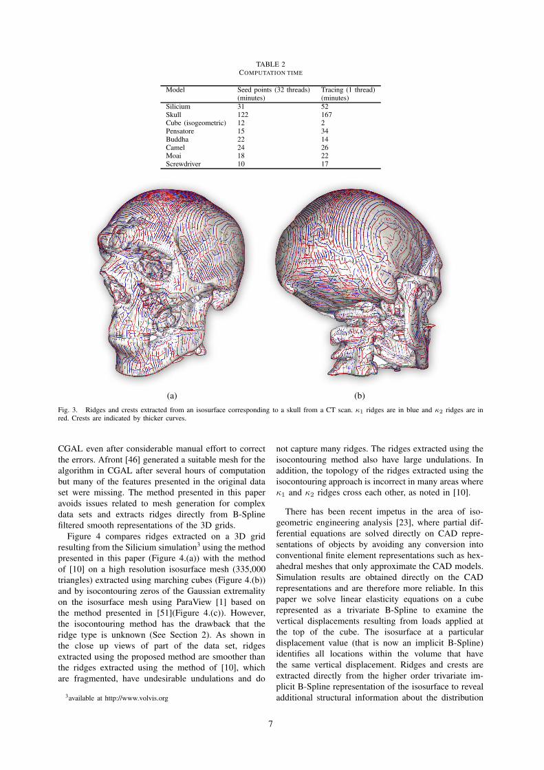
TABLE 2COMPUTATION TIME

Model Seed points (32 threads) Tracing (1 thread)(minutes) (minutes)

Silicium 31 52Skull 122 167Cube (isogeometric) 12 2Pensatore 15 34Buddha 22 14Camel 24 26Moai 18 22Screwdriver 10 17

(a) (b)

Fig. 3. Ridges and crests extracted from an isosurface corresponding to a skull from a CT scan. κ1 ridges are in blue and κ2 ridges are inred. Crests are indicated by thicker curves.

CGAL even after considerable manual effort to correct

the errors. Afront [46] generated a suitable mesh for the

algorithm in CGAL after several hours of computation

but many of the features presented in the original data

set were missing. The method presented in this paper

avoids issues related to mesh generation for complex

data sets and extracts ridges directly from B-Spline

filtered smooth representations of the 3D grids.

Figure 4 compares ridges extracted on a 3D grid

resulting from the Silicium simulation3 using the method

presented in this paper (Figure 4.(a)) with the method

of [10] on a high resolution isosurface mesh (335,000

triangles) extracted using marching cubes (Figure 4.(b))

and by isocontouring zeros of the Gaussian extremality

on the isosurface mesh using ParaView [1] based on

the method presented in [51](Figure 4.(c)). However,

the isocontouring method has the drawback that the

ridge type is unknown (See Section 2). As shown in

the close up views of part of the data set, ridges

extracted using the proposed method are smoother than

the ridges extracted using the method of [10], which

are fragmented, have undesirable undulations and do

3available at http://www.volvis.org

not capture many ridges. The ridges extracted using the

isocontouring method also have large undulations. In

addition, the topology of the ridges extracted using the

isocontouring approach is incorrect in many areas where

κ1 and κ2 ridges cross each other, as noted in [10].

There has been recent impetus in the area of iso-

geometric engineering analysis [23], where partial dif-

ferential equations are solved directly on CAD repre-

sentations of objects by avoiding any conversion into

conventional finite element representations such as hex-

ahedral meshes that only approximate the CAD models.

Simulation results are obtained directly on the CAD

representations and are therefore more reliable. In this

paper we solve linear elasticity equations on a cube

represented as a trivariate B-Spline to examine the

vertical displacements resulting from loads applied at

the top of the cube. The isosurface at a particular

displacement value (that is now an implicit B-Spline)

identifies all locations within the volume that have

the same vertical displacement. Ridges and crests are

extracted directly from the higher order trivariate im-

plicit B-Spline representation of the isosurface to reveal

additional structural information about the distribution

7

(a) (b) (c)

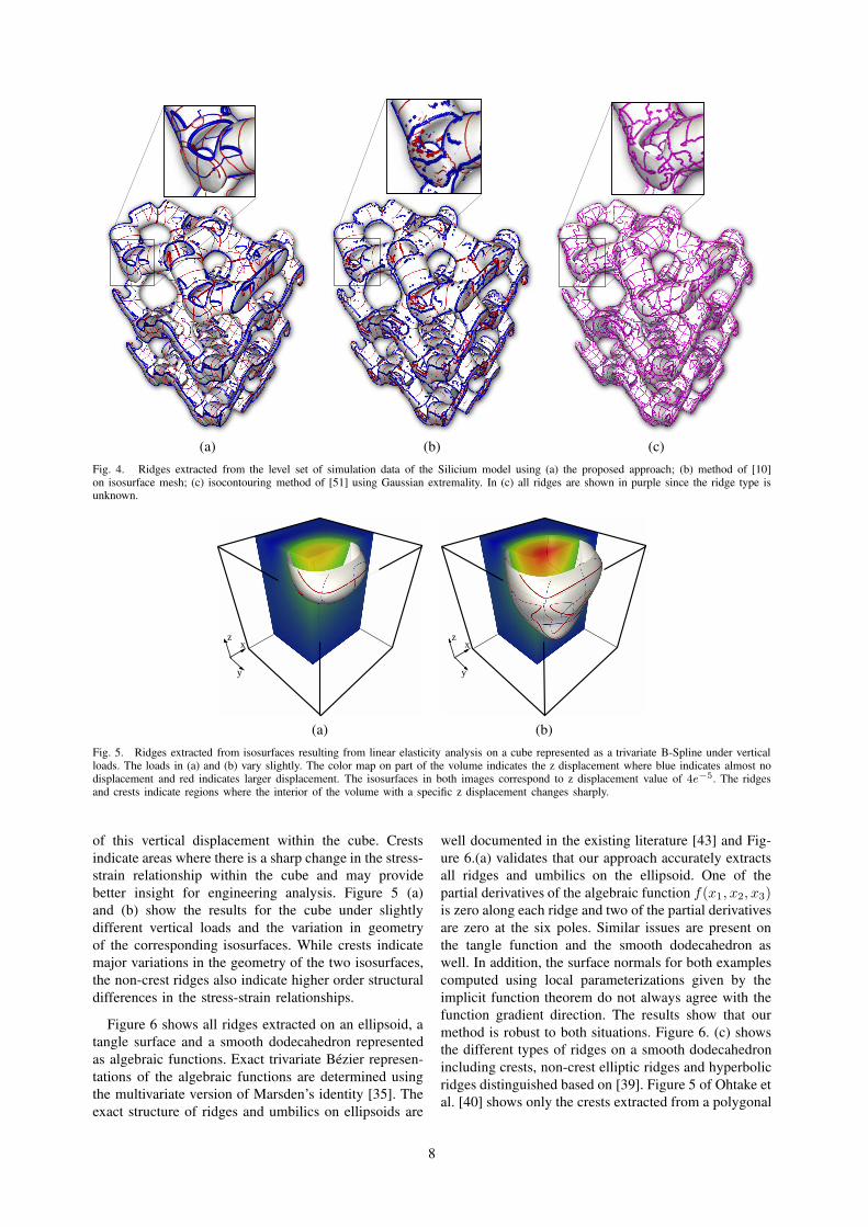
Fig. 4. Ridges extracted from the level set of simulation data of the Silicium model using (a) the proposed approach; (b) method of [10]on isosurface mesh; (c) isocontouring method of [51] using Gaussian extremality. In (c) all ridges are shown in purple since the ridge type isunknown.

zx

y

zx

y

(a) (b)

Fig. 5. Ridges extracted from isosurfaces resulting from linear elasticity analysis on a cube represented as a trivariate B-Spline under verticalloads. The loads in (a) and (b) vary slightly. The color map on part of the volume indicates the z displacement where blue indicates almost nodisplacement and red indicates larger displacement. The isosurfaces in both images correspond to z displacement value of 4e−5. The ridgesand crests indicate regions where the interior of the volume with a specific z displacement changes sharply.

of this vertical displacement within the cube. Crests

indicate areas where there is a sharp change in the stress-

strain relationship within the cube and may provide

better insight for engineering analysis. Figure 5 (a)

and (b) show the results for the cube under slightly

different vertical loads and the variation in geometry

of the corresponding isosurfaces. While crests indicate

major variations in the geometry of the two isosurfaces,

the non-crest ridges also indicate higher order structural

differences in the stress-strain relationships.

Figure 6 shows all ridges extracted on an ellipsoid, a

tangle surface and a smooth dodecahedron represented

as algebraic functions. Exact trivariate Bezier represen-

tations of the algebraic functions are determined using

the multivariate version of Marsden’s identity [35]. The

exact structure of ridges and umbilics on ellipsoids are

well documented in the existing literature [43] and Fig-

ure 6.(a) validates that our approach accurately extracts

all ridges and umbilics on the ellipsoid. One of the

partial derivatives of the algebraic function f(x1, x2, x3)is zero along each ridge and two of the partial derivatives

are zero at the six poles. Similar issues are present on

the tangle function and the smooth dodecahedron as

well. In addition, the surface normals for both examples

computed using local parameterizations given by the

implicit function theorem do not always agree with the

function gradient direction. The results show that our

method is robust to both situations. Figure 6. (c) shows

the different types of ridges on a smooth dodecahedron

including crests, non-crest elliptic ridges and hyperbolic

ridges distinguished based on [39]. Figure 5 of Ohtake et

al. [40] shows only the crests extracted from a polygonal

8

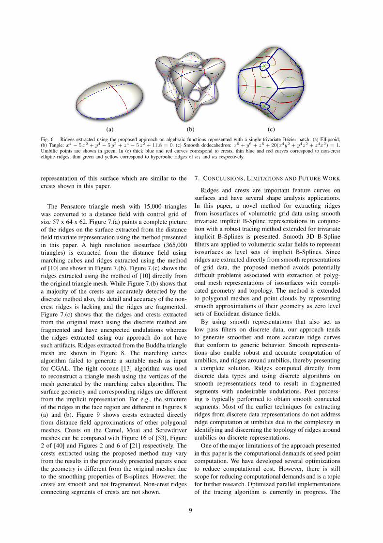
(a) (b) (c)

Fig. 6. Ridges extracted using the proposed approach on algebraic functions represented with a single trivariate Bezier patch: (a) Ellipsoid;(b) Tangle: x4

− 5x2 + y4 − 5 y2 + z4 − 5 z2 + 11.8 = 0. (c) Smooth dodecahedron: x6 + y6 + z6 + 20(x4y2 + y4z2 + z4x2) = 1.Umbilic points are shown in green. In (c) thick blue and red curves correspond to crests, thin blue and red curves correspond to non-crestelliptic ridges, thin green and yellow correspond to hyperbolic ridges of κ1 and κ2 respectively.

representation of this surface which are similar to the

crests shown in this paper.

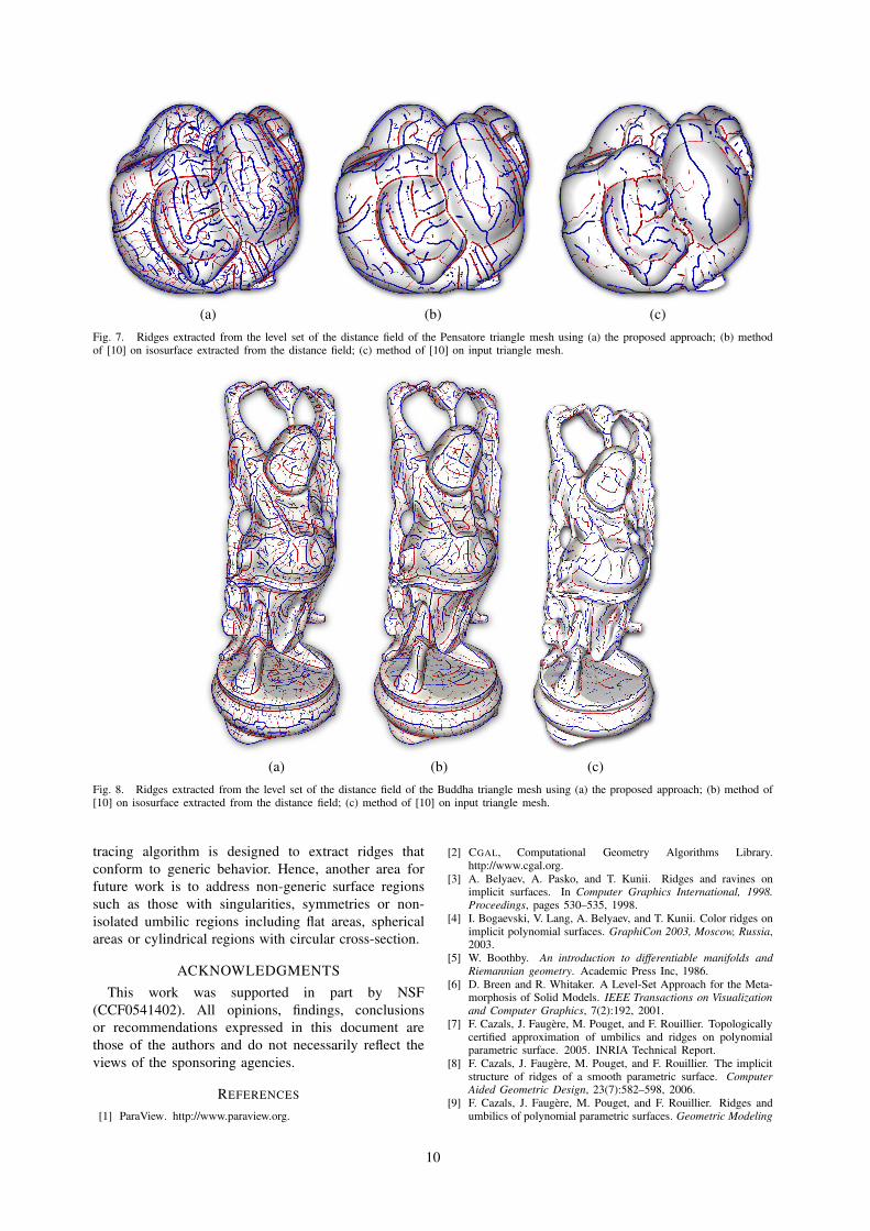
The Pensatore triangle mesh with 15,000 triangles

was converted to a distance field with control grid of

size 57 x 64 x 62. Figure 7.(a) paints a complete picture

of the ridges on the surface extracted from the distance

field trivariate representation using the method presented

in this paper. A high resolution isosurface (365,000

triangles) is extracted from the distance field using

marching cubes and ridges extracted using the method

of [10] are shown in Figure 7.(b). Figure 7.(c) shows the

ridges extracted using the method of [10] directly from

the original triangle mesh. While Figure 7.(b) shows that

a majority of the crests are accurately detected by the

discrete method also, the detail and accuracy of the non-

crest ridges is lacking and the ridges are fragmented.

Figure 7.(c) shows that the ridges and crests extracted

from the original mesh using the discrete method are

fragmented and have unexpected undulations whereas

the ridges extracted using our approach do not have

such artifacts. Ridges extracted from the Buddha triangle

mesh are shown in Figure 8. The marching cubes

algorithm failed to generate a suitable mesh as input

for CGAL. The tight cocone [13] algorithm was used

to reconstruct a triangle mesh using the vertices of the

mesh generated by the marching cubes algorithm. The

surface geometry and corresponding ridges are different

from the implicit representation. For e.g., the structure

of the ridges in the face region are different in Figures 8

(a) and (b). Figure 9 shows crests extracted directly

from distance field approximations of other polygonal

meshes. Crests on the Camel, Moai and Screwdriver

meshes can be compared with Figure 16 of [53], Figure

2 of [40] and Figures 2 and 6 of [21] respectively. The

crests extracted using the proposed method may vary

from the results in the previously presented papers since

the geometry is different from the original meshes due

to the smoothing properties of B-splines. However, the

crests are smooth and not fragmented. Non-crest ridges

connecting segments of crests are not shown.

7. CONCLUSIONS, LIMITATIONS AND FUTURE WORK

Ridges and crests are important feature curves on

surfaces and have several shape analysis applications.

In this paper, a novel method for extracting ridges

from isosurfaces of volumetric grid data using smooth

trivariate implicit B-Spline representations in conjunc-

tion with a robust tracing method extended for trivariate

implicit B-Splines is presented. Smooth 3D B-Spline

filters are applied to volumetric scalar fields to represent

isosurfaces as level sets of implicit B-Splines. Since

ridges are extracted directly from smooth representations

of grid data, the proposed method avoids potentially

difficult problems associated with extraction of polyg-

onal mesh representations of isosurfaces with compli-

cated geometry and topology. The method is extended

to polygonal meshes and point clouds by representing

smooth approximations of their geometry as zero level

sets of Euclidean distance fields.

By using smooth representations that also act as

low pass filters on discrete data, our approach tends

to generate smoother and more accurate ridge curves

that conform to generic behavior. Smooth representa-

tions also enable robust and accurate computation of

umbilics, and ridges around umbilics, thereby presenting

a complete solution. Ridges computed directly from

discrete data types and using discrete algorithms on

smooth representations tend to result in fragmented

segments with undesirable undulations. Post process-

ing is typically performed to obtain smooth connected

segments. Most of the earlier techniques for extracting

ridges from discrete data representations do not address

ridge computation at umbilics due to the complexity in

identifying and discerning the topology of ridges around

umbilics on discrete representations.

One of the major limitations of the approach presented

in this paper is the computational demands of seed point

computation. We have developed several optimizations

to reduce computational cost. However, there is still

scope for reducing computational demands and is a topic

for further research. Optimized parallel implementations

of the tracing algorithm is currently in progress. The

9

(a) (b) (c)

Fig. 7. Ridges extracted from the level set of the distance field of the Pensatore triangle mesh using (a) the proposed approach; (b) methodof [10] on isosurface extracted from the distance field; (c) method of [10] on input triangle mesh.

(a) (b) (c)

Fig. 8. Ridges extracted from the level set of the distance field of the Buddha triangle mesh using (a) the proposed approach; (b) method of[10] on isosurface extracted from the distance field; (c) method of [10] on input triangle mesh.

tracing algorithm is designed to extract ridges that

conform to generic behavior. Hence, another area for

future work is to address non-generic surface regions

such as those with singularities, symmetries or non-

isolated umbilic regions including flat areas, spherical

areas or cylindrical regions with circular cross-section.

ACKNOWLEDGMENTS

This work was supported in part by NSF

(CCF0541402). All opinions, findings, conclusions

or recommendations expressed in this document are

those of the authors and do not necessarily reflect the

views of the sponsoring agencies.

REFERENCES

[1] ParaView. http://www.paraview.org.

[2] CGAL, Computational Geometry Algorithms Library.http://www.cgal.org.

[3] A. Belyaev, A. Pasko, and T. Kunii. Ridges and ravines onimplicit surfaces. In Computer Graphics International, 1998.

Proceedings, pages 530–535, 1998.

[4] I. Bogaevski, V. Lang, A. Belyaev, and T. Kunii. Color ridges onimplicit polynomial surfaces. GraphiCon 2003, Moscow, Russia,2003.

[5] W. Boothby. An introduction to differentiable manifolds and

Riemannian geometry. Academic Press Inc, 1986.

[6] D. Breen and R. Whitaker. A Level-Set Approach for the Meta-morphosis of Solid Models. IEEE Transactions on Visualization

and Computer Graphics, 7(2):192, 2001.

[7] F. Cazals, J. Faugere, M. Pouget, and F. Rouillier. Topologicallycertified approximation of umbilics and ridges on polynomialparametric surface. 2005. INRIA Technical Report.

[8] F. Cazals, J. Faugere, M. Pouget, and F. Rouillier. The implicitstructure of ridges of a smooth parametric surface. ComputerAided Geometric Design, 23(7):582–598, 2006.

[9] F. Cazals, J. Faugere, M. Pouget, and F. Rouillier. Ridges andumbilics of polynomial parametric surfaces. Geometric Modeling

10

(a) (b) (c)

Fig. 9. Crests extracted from the level set of the distance field of the (a) Camel mesh; (b) Moai mesh; (c) Screwdriver mesh.

and Algebraic Geometry, pages 141–159, 2007. Juttler, B. andPiene, R. (eds.).

[10] F. Cazals and M. Pouget. Topology driven algorithms for ridgeextraction on meshes. 2005. INRIA Technical Report.

[11] E. Cohen, R. F. Riesenfeld, and G. Elber. Geometric modelingwith splines: an introduction. A. K. Peters, Ltd., Natick, MA,USA, 2001.

[12] F. Cole, A. Golovinskiy, A. Limpaecher, H. S. Barros, A. Finkel-stein, T. Funkhouser, and S. Rusinkiewicz. Where do peopledraw lines? ACM Transactions on Graphics (Proc. SIGGRAPH),27(3), Aug. 2008.

[13] T. Dey and S. Goswami. Tight cocone: a water-tight surfacereconstructor. Journal of Computing and Information Science inEngineering, 3:302, 2003.

[14] M. Do Carmo. Differential geometry of curves and surfaces.Prentice-Hall Englewood Cliffs, NJ, 1976.

[15] D. Eberly. Ridges in image and data analysis. Kluwer AcademicPub, 1996.

[16] G. Elber. The IRIT modeling environment, version 10.0, 2008.

[17] G. Elber and T. Grandine. Efficient solution to systems ofmultivariate polynomials using expression trees. In IEEE Inter-

national Conference on Shape Modeling and Applications, 2008.

SMI 2008, pages 163–169, 2008.

[18] G. Elber and M. Kim. Geometric constraint solver usingmultivariate rational spline functions. In Proceedings of the sixth

ACM symposium on Solid modeling and applications, pages 1–10. ACM New York, NY, USA, 2001.

[19] A. Gueziec. Large deformable splines, crest lines and matching.In Computer Vision, 1993. Proceedings., Fourth International

Conference on, pages 650–657, 1993.

[20] P. Hallinan, G. Gordon, A. Yuille, P. Giblin, and D. Mumford.Two-and three-dimensional patterns of the face. AK Peters, Ltd.Natick, MA, USA, 1999.

[21] K. Hildebrandt, K. Polthier, and M. Wardetzky. Smooth featurelines on surface meshes. In Symposium on geometry processing,pages 85–90, 2005.

[22] M. Hosaka. Modeling of curves and surfaces in CAD/CAM.Springer, 1992.

[23] T. Hughes, J. Cottrell, and Y. Bazilevs. Isogeometric analy-sis: CAD, finite elements, NURBS, exact geometry and meshrefinement. Computer Methods in Applied Mechanics and

Engineering, 194(39-41):4135–4195, 2005.

[24] V. Interrante, H. Fuchs, and S. Pizer. Enhancing transparentskin surfaces with ridge and valley lines. In Proceedings ofthe 6th conference on Visualization’95. IEEE Computer SocietyWashington, DC, USA, 1995.

[25] M. Jefferies. Extracting Crest Lines from B-spline Surfaces.Arizona State University, 2002.

[26] J. Kent, K. Mardia, and J. West. Ridge curves and shape analysis.In The British Machine Vision Conference 1996, pages 43–52,1996.

[27] S. Kim and C. Kim. Finding ridges and valleys in a discretesurface using a modified MLS approximation. Computer-Aided

Design, 37(14):1533–1542, 2005.

[28] K. Ko, T. Maekawa, N. Patrikalakis, H. Masuda, and F. Wolter.Shape intrinsic fingerprints for free-form object matching. InProceedings of the eighth ACM symposium on Solid modeling

and applications, pages 196–207. ACM New York, NY, USA,2003.

[29] J. Little and P. Shi. Structural lines, TINs, and DEMs. Algorith-mica, 30(2):243–263, 2001.

[30] W. Lorensen and H. Cline. Marching cubes: A high resolution3D surface construction algorithm. In Proceedings of the14th annual conference on Computer graphics and interactive

techniques, page 169. ACM, 1987.

[31] K. Ma and V. Interrante. Extracting feature lines from 3Dunstructured grids. In Visualization’97., Proceedings, pages 285–292, 1997.

[32] T. Maekawa and N. Patrikalakis. Interrogation of differentialgeometry properties for design and manufacture. The Visual

Computer, 10(4):216–237, 1994.

[33] T. Maekawa, F. Wolter, and N. Patrikalakis. Umbilics and linesof curvature for shape interrogation. Computer Aided Geometric

Design, 13(2):133–161, 1996.

[34] S. R. Marschner and R. J. Lobb. An evaluation of reconstructionfilters for volume rendering. In VIS ’94: Proceedings of theconference on Visualization ’94, pages 100–107, Los Alamitos,CA, USA, 1994. IEEE Computer Society Press.

[35] M. J. Marsden. An identity for spline functions with applicationsto variation diminishing spline approximation. J. Approx. Theory,3:7–49, 1970.

[36] J. Maxwell. L. On hills and dales. Philosophical Magazine

Series 4, 40(269):421–427, 1870.

[37] O. Monga and S. Benayoun. Using partial derivatives of 3Dimages to extract typical surface features. Computer Vision and

Image Understanding, 61(2):171–189, 1995.

[38] R. Morris. Symmetry of Curves and the Geometry of Surfaces.PhD thesis, PhD thesis, University of Liverpool, 1990.

[39] S. Musuvathy, E. Cohen, J. Seong, and J. Damon. Tracing Ridgeson B-Spline Surfaces. In Proceedings of the SIAM/ACM Joint

Conference on Geometric and Physical Modeling, 2009.

[40] Y. Ohtake, A. Belyaev, and H. Seidel. Ridge-valley lineson meshes via implicit surface fitting. ACM Transactions on

Graphics, 23(3):609–612, 2004.

[41] N. Patrikalakis and T. Maekawa. Shape interrogation for

computer aided design and manufacturing. Springer, 2002.

[42] X. Pennec, N. Ayache, and J.-P. Thirion. Landmark-based regis-tration using features identified through differential geometry. InI. Bankman, editor, Handbook of Medical Image Processing andAnalysis - New edition, chapter 34, pages 565–578. AcademicPress, Dec. 2008.

[43] I. Porteous. Geometric differentiation: for the intelligence ofcurves and surfaces. Cambridge University Press, 2001.

[44] A. Raviv and G. Elber. Three dimensional freeform sculpting viazero sets of scalar trivariate functions. In SMA ’99: Proceedings

of the fifth ACM symposium on Solid modeling and applications,pages 246–257, New York, NY, USA, 1999. ACM.

11

[45] A. Rockwood. Accurate display of tensor product isosurfaces.In Proceedings of the 1st conference on Visualization’90, page360. IEEE Computer Society Press, 1990.

[46] J. Schreiner, C. Scheidegger, and C. Silva. High quality ex-traction of isosurfaces from regular and irregular grids. IEEE

Transactions on Visualization and Computer Graphics (Proceed-ings Visualization / Information Visualization 2006), 12(5):1205–1212, September-October 2006.

[47] O. Soldea. Global segmentation and curvature analysis of volu-metric data sets using trivariate b-spline functions. IEEE Trans.Pattern Anal. Mach. Intell., 28(2):265–278, 2006. Member-Elber,Gershon and Member-Rivlin, Ehud.

[48] G. Stylianou and G. Farin. Crest lines extraction from 3Dtriangulated meshes. Hierarchical and geometrical methods inscientific visualization, pages 269–281, 2003.

[49] G. Subsol. Crest lines for curve-based warping. Brain Warping,pages 241–262, 1999.

[50] T. Tasdizen and R. Whitaker. Feature preserving variationalsmoothing of terrain data. In Proceedings of the Second IEEEWorkshop on Variational, Geometric and Level Set Methods in

Computer Vision (VLSM’03)(Institute of Electrical and Electron-

ics Engineers, 2003), pages 121–128.[51] J. Thirion. The extremal mesh and the understanding of 3D

surfaces. International Journal of Computer Vision, 19(2):115–128, 1996.

[52] J. Thirion and A. Gourdon. The 3D marching lines algorithmand its application to crest lines extraction. 1992.

[53] S. Yoshizawa, A. Belyaev, H. Yokota, and H. Seidel. Fast andfaithful geometric algorithm for detecting crest lines on meshes.In Computer Graphics and Applications, 2007. PG’07. 15th

Pacific Conference on, pages 231–237, 2007.

APPENDIX A

INVARIANCE OF CREST CONDITIONS

In the neighborhood of any point p on a surface

S(u, v), define σi(u, v) = (u, v, κi(u, v)) i = 1 or

2, where κi is a principal curvature of S(u, v). Let

ti = [ti1 ti2]T such that Ti = ti1Su + ti2Sv is

the principal direction corresponding to κi. Then the

second fundamental form of the surface σi(u, v) in the

ti direction is

IIp(ti) = tTi

[

〈σiuu, nσi〉 〈σiuv , nσi

〉〈σivu, nσi

〉 〈σivv , nσi〉

]

ti

= tTi

[

κiuu κiuv

κiuv κivv

]

ti

(12)

Since the second fundamental form of a surface

is invariant under coordinate transformations [14], the

invariance of the crest conditions follows.

APPENDIX B

DIFFERENTIAL PROPERTIES OF ISOSURFACES

This section summarizes formulae for computing

principal curvatures, principal directions and curvature

gradients of an isosurface (See [47], [52] for details).

Let f(x1, x2, x3) : R3 7−→ R, f ∈ C(4). I =(x1, x2, x3) : f(x1, x2, x3) = a is an isosurface.

Assuming fx36= 0, I can be locally represented as

S(x1, x2) = (x1, x2, g(x1, x2)).

n = Sx1× Sx2

= (fx1

fx3

,fx2

fx3

, 1) (13)

We assume that the surface normal n(x1, x2) of

S(x1, x2) is oriented toward the interior of the region

bounded by S(x1, x2).

The coefficients of the first fundamental form are

given by,

E = 1+f2x1

f2x3

;F =fx1

fx2

f2x3

;G = 1 +f2x2

f2x3

(14)

The coefficients of the second fundamental form are

given by,

L =(2fx1

fx3fx1x3

− fx1x1f2x3

− f2x1fx3x3

)

f2x3

√

f2x1

+ f2x2

+ f2x3

(15)

M = ((fx1fx3

fx2x3+ fx2

fx3fx1x3

−fx1

fx2fx3x3

− f2x3fx1x2

))/

(f2x3

√

f2x1

+ f2x2

+ f2x3)

(16)

N =(2fx2

fx3fx2x3

− f2x2fx3x3

− f2x3fx2x2

)

f2x3

√

f2x1

+ f2x2

+ f2x3

(17)

The principal curvatures, κi, i = 1, 2 are the roots of

the following quadratic equation as given in [11]:

aκ2 + bκ+ c = 0a = EG− F 2

b = 2FM −GL− ENc = LN −M2

(18)

κ1 =−b+

√b2 − 4ac

2a;κ2 =

−b−√b2 − 4ac

2a(19)

a =f2x1

+ f2x2

+ f2x3

f2x3

(20)

b = (fx1x1(f2

x2+ f2

x3) + fx2x2

(f2x1

+ f2x3)+

fx3x3(f2

x1+ f2

x2)− 2fx1

fx2fx1x2

−2fx2

fx3fx2x3

− 2fx3fx1

fx1x3)/

(f2x3

√

f2x1

+ f2x2

+ f2x3)

(21)

c = (f2x1(fx2x2

fx3x3− f2

x2x3) + f2

x2(fx3x3

fx1x1− f2

x1x3)+

f2x3(fx1x1

fx2x2− f2

x1x2)+

2fx1fx2

(fx1x3fx2x3

− fx1x2fx3x3

)+

2fx1fx3

(fx1x2fx2x3

− fx1x3fx2x2

)+

2fx2fx3

(fx1x3fx1x2

− fx1x1fx2x3

))/

(f2x3(f2

x1+ f2

x2+ f2

x3))

(22)

ti =

[

−(M − κiF )L− κiE)

]

or

[

−(N − κiG)M − κiF )

]

i = 1, 2 (23)

∇κi =[

κix1κix2

]T(24)

κix1(x1, x2, g(x1, x2)) = κix1

(x1, x2, x3)−

κix3(x1, x2, x3)(

fx1

fx3

)(25)

12

κix2(x1, x2, g(x1, x2)) = κix2

(x1, x2, x3)−

κix3(x1, x2, x3)(

fx2

fx3

)(26)

13