Riemann–Hilbert problem for bi-orthogonal polynomials

This article has been downloaded from IOPscience. Please scroll down to see the full text article.

2003 J. Phys. A: Math. Gen. 36 4629

(http://iopscience.iop.org/0305-4470/36/16/312)

Download details:

IP Address: 66.194.72.152

The article was downloaded on 15/09/2013 at 09:20

Please note that terms and conditions apply.

View the table of contents for this issue, or go to the journal homepage for more

Home Search Collections Journals About Contact us My IOPscience

INSTITUTE OF PHYSICS PUBLISHING JOURNAL OF PHYSICS A: MATHEMATICAL AND GENERAL

J. Phys. A: Math. Gen. 36 (2003) 4629–4640 PII: S0305-4470(03)54680-7

Riemann–Hilbert problem for bi-orthogonalpolynomials

Andrei A Kapaev

St Petersburg Department of Steklov Mathematical Institute of Russian Academy of Sciences,Fontanka 27, St Petersburg, 191011, Russia

E-mail: kapaev@pdmi.ras.ru

Received 9 October 2002, in final form 4 March 2003Published 8 April 2003Online at stacks.iop.org/JPhysA/36/4629

AbstractThe 3 × 3 matrix Riemann–Hilbert problem for bi-orthogonal polynomialswith the third-degree polynomial potential functions is explicitly constructed.The developed approach can be extended to bi-orthogonal polynomials witharbitrary polynomial potentials.

PACS numbers: 02.30.Zz, 02.30.GpMathematics Subject Classification: 34M50, 34M40

1. Introduction

The classical asymptotic theory of orthogonal polynomials [1, 2] extended to polynomialsorthogonal with respect to the weight exp(−NV (z)) [3–6] has gained essential progress afterintroduction of the Riemann–Hilbert (RH) problem approach [7] and the steepest descentmethod [8]. A particular implementation of these methods to the orthogonal polynomials onthe real line can by found in [9, 10] while orthogonal polynomials on the circle are studiedin [11].

Further extensions of the notion of orthogonal polynomials motivated by a number ofapplications to the random matrix theory, integrable systems, approximation theory andcombinatorics include generalized orthogonal polynomials and bi-orthogonal polynomials.In the former case, the sequence of polynomials is orthogonal with respect to a sequence ofmeasures [12, 13]∫

R

Pn(λ) dρm(λ) = δnm

while in the latter case, two sequences of polynomials are orthogonal to each other with respectto a two-dimensional measure [14–16],∫

R

∫R

Pn(λ)Qm(ξ) dµ(λ, ξ) = δnm.

0305-4470/03/164629+12$30.00 © 2003 IOP Publishing Ltd Printed in the UK 4629

4630 A A Kapaev

In the simplest case, the two-dimensional measure has the form of the product dµ(λ, ξ) =exp(−V (λ)−W(ξ) + λξ) dλ dξ where the polynomials V (λ) andW(ξ) are called potentials.Integration over ξ in the latter two-fold integral yields the sequence of measures, dρm(λ) =φm(λ) dλ = ∫

RQm(ξ) dµ(λ, ξ). The functions φm(λ) here are called dual functions [15].

Generalized and bi-orthogonal polynomials are associated with a completely integrablesystem coming from t-deformations and Virasoro constraints and typically describing certainreductions of the 2-Toda lattice [12–16]. However, although the algebraic properties ofthe generalized and bi-orthogonal polynomials are extensively studied, knowledge of theasymptotic properties of such polynomials is limited. Basically, this is due to the absence ofan adequate formulation of the relevant RH problem. Indeed, even though the 2 × 2 matrixRH problem formulation for the conventional orthogonal polynomials [7] admits a direct 2×2extension to the case of generalized orthogonal polynomials [12], the relevant version forbi-orthogonal polynomials [14] exhibits its non-local nature.

Fortunately, recent study reveals the isomonodromy structure associated with bi-orthogonal polynomials and hence the principal possibility of formulating an n × n matrixRH problem which would have properties similar to those for the 2 × 2 matrix RH problemfor conventional orthogonal polynomials [15]. In what follows, assuming the existence of bi-orthogonal polynomials for the third-degree polynomial potentials, we construct the relevant3 × 3 matrix RH problem, as well as the 3 × 3 RH problem for the dual functions. In spite ofits less physical importance, this case provides us the opportunity to develop the technique inthe simplest non-trivial case. (The bi-orthogonal polynomials for the second-degree potentialsare reduced to classical Hermite polynomials [14]. In some more involved cases such asdegV (λ) > 2, degW(ξ) = 2, the bi-orthogonal polynomials can be expressed in terms ofsemi-classical orthogonal polynomials related to the 2 × 2 matrix RH problem studied in[7, 9–11] and other papers.

We stress that the method explained below can be extended to arbitrary polynomialpotentials. We also point out a particular importance of the paper [17] which is useful for theconstruction and justification of the RH problem for the dual functions in the class of weightswith rational log derivatives.

After the original version of the present paper was posted on the Internet [18], the Montrealgroup presented their methodology for constructing a similar RH problem [19]. Their idea forevaluation of the RH problem for the dual functions based on the study of path integrals concurswith ours but, in contrast to our cubic case, they consider arbitrary polynomial potentials. Asfor the RH problem for the original (wave) function, the authors of [19] rely on the so-calledduality pairing, while our approach is based on the explicit integral representation of thewavefunction.

This paper is organized as follows. In section 2, we recall the matrix differential anddifference equations satisfied by the bi-orthogonal polynomials and their dual functions. Insection 3, we construct fundamental solutions for the differential–difference system for thedual functions which gives rise to the RH problem (equations (22)–(24)) for the dual functions.In section 4, we construct fundamental solutions of the differential–difference system for thebi-orthogonal polynomials and the relevant RH problem (equations (37)–(39)). In section 5,we discuss some properties and implications of the constructed RH problems.

2. Equations for the bi-orthogonal polynomials

Below, we consider monic polynomials pn(λ), qm(ξ) satisfying the orthogonality condition∫γ1

dλ∫γ2

dξpn(λ)qm(ξ) exp(−V (λ)−W(ξ) + tλξ) = h2nδn,m (1)

Riemann–Hilbert problem for bi-orthogonal polynomials 4631

where

V (λ) = 13λ

3 + xλ W(ξ) = 13 ξ

3 + yξ

x, y, t ∈ C, t �= 0; the contours γi, i = 1, 2, are the complex linear combinations of theelementary contours,

γi =2∑j=0

g(i)j �j g

(i)j ∈ C i = 1, 2 (2)

where each �j is the sum of two rays

�j = (exp

(i 2π

3 (j − 2))∞, 0

] ∪ [0, exp

(i 2π

3 (j − 1))∞)

j = 0, 1, 2. (3)

Because �0 + �1 + �2 = 0, one of the parameters, g(1)j (respectively g(2)j ), can be put to

zero and one of the nontrivial parameters, g(i)j , can be normalized to unity. Thus the set ofcontours γj and, therefore, the set of monic bi-orthogonal polynomials are parametrized bythree constant complex parameters. (More general parametrization of the set of contours isintroduced in [19]; however, in our cubic case, both kinds of parametrization are equivalent.We also note that the general cubic potentials can be reduced to the above form using the lineartransformations in λ and ξ .)

We introduce the wavefunctions

ψn(λ) = 1

hnpn(λ) exp(−V (λ)) φm(ξ) = 1

hmqm(ξ) exp(−W(ξ)) (4)

and their Fourier–Laplace images ψn(ξ), φm(λ) called the dual functions [15],

ψn(ξ) =∫γ1

ψn(λ) exp(tλξ) dλ φm(λ) =∫γ2

φm(ξ) exp(tλξ) dξ. (5)

The orthogonality condition (1) now reads∫γ1

dλ∫γ2

dξψn(λ)φm(ξ) exp(tλξ) =∫γ1

ψn(λ)φm(λ) dλ =∫γ2

ψn(ξ)φm(ξ) dξ = δnm. (6)

It implies certain relations between the introduced functions (4) and (5). We refer to [15] forthe general case and present the final result for our particular situation here:

λψn(λ) =n+1∑

m=n−2

an,mψm(λ) ∂λψn(λ) = −tn+2∑

m=n−1

bn,mψm(λ)

∂xψn(λ) =n+1∑m=n

un,mψm(λ) ∂yψn(λ) = −n∑

m=n−1

vn,mψm(λ) (7)

∂tψn(λ) = wnψn(λ)−n−1∑

m=n−3

An,mψm(λ)

ξφm(ξ) =m+1∑

n=m−2

bn,mφn(ξ) ∂ξφm(ξ) = −tm+2∑

n=m−1

an,mφn(ξ)

∂yφm(ξ) =m+1∑n=m

vn,mφn(ξ) ∂xφm(ξ) = −m∑

n=m−1

un,mφn(ξ) (8)

∂tφm(ξ) = wmφm(ξ)−m−1∑n=m−3

An,mφn(ξ)

where the coefficients an,m, bn,m, un,m, vn,m,An,m are described in more detail in [18].

4632 A A Kapaev

Using definition (5) and the equations given above, it is straightforward that the dualfunctions satisfy equations

∂ξ ψn(ξ) =n+1∑

m=n−2

tan,mψm(ξ) ξψn(ξ) =n+2∑

m=n−1

bn,mψm(ξ)

∂xψn(ξ) =n+1∑m=n

un,mψm(ξ) ∂yψn(ξ) = −n∑

m=n−1

vn,mψm(ξ) (9)

∂t ψn(ξ) = −wnψn(ξ) +n+3∑

m=n+1

An,mψm(ξ)

∂λφm(λ) =m+1∑

n=m−2

tbn,mφn(λ) λφm(λ) =m+2∑

n=m−1

an,mφn(λ)

∂yφm(λ) =m+1∑n=m

vn,mφn(λ) ∂xφm(λ) = −m∑

n=m−1

un,mφn(λ) (10)

∂t φm(λ) = −wmφm(λ) +m+3∑n=m+1

An,mφn(λ).

Using the above equations, 3-vectors �n(λ) = (ψn(λ), ψn−1(λ), ψn−2(λ))T , �m(ξ) =

(φm(ξ), φm−1(ξ), φm−2(ξ))T , and dual vectors ψn(ξ) = (ψn(ξ), ψn−1(ξ), ψn−2(ξ))

T ,φm(λ) = (φm(λ), φm−1(λ), φm−2(λ))

T satisfy the following systems of difference anddifferential equations with 3 × 3 matrix coefficients [15],

�n+1(λ) = Rn(λ)�n(λ)∂�n

∂λ(λ) = An(λ)�n(λ)

(11)∂�n

∂x= Un(λ)�n

∂�n

∂y= Vn(λ)�n

∂�n

∂t= Wn(λ)�n

�m+1(ξ) = Qm(ξ)�m(ξ)∂�m

∂ξ(ξ) = Bm(ξ)�m(ξ)

(12)∂�m

∂x= Um�m

∂�m

∂y= Vm�m

∂�m

∂t= Wm�m

�n+1(ξ) = Rn(ξ)�n(ξ)∂�n

∂ξ(ξ) = An(ξ)�n(ξ)

(13)∂�n

∂x(ξ) = Un(ξ)�n(ξ)

∂�n

∂y(ξ) = Vn(ξ)�n(ξ)

∂�n

∂t(ξ) = Wn(ξ)�n(ξ)

�m+1(λ) = Qm(λ)�m(λ)∂�m

∂λ(λ) = Bm(λ)�m(λ)

(14)∂�m

∂x(λ) = Um(λ)�m(λ)

∂�m

∂y(λ) = Vm(λ)�m(λ)

∂�m

∂t(λ) = Wm(λ)�m(λ)

where the expressions for the 3 × 3 matrix coefficients are given in [18].The compatibility conditions of the above equations yield a reduction of the 2-Toda lattice

[12]. On the other hand, this nonlinear system describes the isomonodromy deformations withrespect to the parameters x, y, t ∈ C and n,m ∈ N of the 3 × 3 matrix differential equations

Riemann–Hilbert problem for bi-orthogonal polynomials 4633

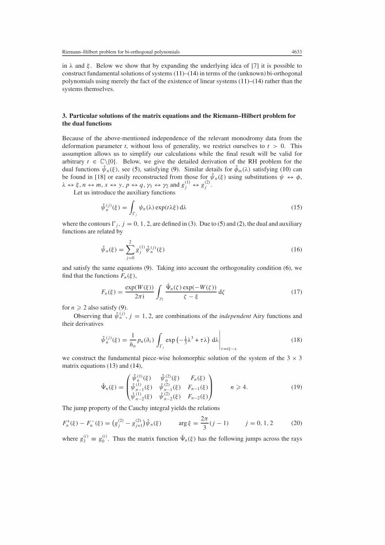
in λ and ξ . Below we show that by expanding the underlying idea of [7] it is possible toconstruct fundamental solutions of systems (11)–(14) in terms of the (unknown) bi-orthogonalpolynomials using merely the fact of the existence of linear systems (11)–(14) rather than thesystems themselves.

3. Particular solutions of the matrix equations and the Riemann–Hilbert problem forthe dual functions

Because of the above-mentioned independence of the relevant monodromy data from thedeformation parameter t, without loss of generality, we restrict ourselves to t > 0. Thisassumption allows us to simplify our calculations while the final result will be valid forarbitrary t ∈ C\{0}. Below, we give the detailed derivation of the RH problem for thedual functions ψn(ξ), see (5), satisfying (9). Similar details for φm(λ) satisfying (10) canbe found in [18] or easily reconstructed from those for ψn(ξ) using substitutions ψ ↔ φ,λ ↔ ξ, n ↔ m, x ↔ y, p ↔ q , γ1 ↔ γ2 and g(1)j ↔ g

(2)j .

Let us introduce the auxiliary functions

ψ(j)n (ξ) =

∫�j

ψn(λ) exp(tλξ) dλ (15)

where the contours�j , j = 0, 1, 2, are defined in (3). Due to (5) and (2), the dual and auxiliaryfunctions are related by

ψn(ξ) =2∑j=0

g(1)j ψ

(j)n (ξ) (16)

and satisfy the same equations (9). Taking into account the orthogonality condition (6), wefind that the functions Fn(ξ),

Fn(ξ) = exp(W(ξ))

2π i

∫γ2

�n(ζ ) exp(−W(ζ ))ζ − ξ

dζ (17)

for n � 2 also satisfy (9).Observing that ψ(j)

n , j = 1, 2, are combinations of the independent Airy functions andtheir derivatives

ψ(j)n (ξ) = 1

hnpn(∂τ )

∫�j

exp(− 1

3λ3 + τλ

)dλ

∣∣∣∣∣τ=tξ−x

(18)

we construct the fundamental piece-wise holomorphic solution of the system of the 3 × 3matrix equations (13) and (14),

�n(ξ) =

ψ(1)n (ξ) ψ(2)

n (ξ) Fn(ξ)

ψ(1)n−1(ξ) ψ

(2)n−1(ξ) Fn−1(ξ)

ψ(1)n−2(ξ) ψ

(2)n−2(ξ) Fn−2(ξ)

n � 4. (19)

The jump property of the Cauchy integral yields the relations

F +n (ξ)− F−

n (ξ) = (g(2)j − g

(2)j+1

)ψn(ξ) arg ξ = 2π

3(j − 1) j = 0, 1, 2 (20)

where g(i)3 ≡ g(i)0 . Thus the matrix function �n(ξ) has the following jumps across the rays

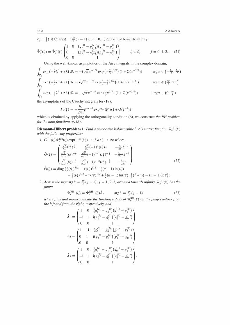
4634 A A Kapaev

�j = {ξ ∈ C: arg ξ = 2π

3 (j − 1)}, j = 0, 1, 2, oriented towards infinity

�+n (ξ) = �−

n (ξ)

1 0(g(2)j − g

(2)j+1

)(g(1)1 − g

(1)0

)0 1

(g(2)j − g

(2)j+1

)(g(1)2 − g

(1)0

)0 0 1

ξ ∈ �j j = 0, 1, 2. (21)

Using the well-known asymptotics of the Airy integrals in the complex domain,∫�0

exp(− 1

3λ3 + τλ

)dλ = −i

√πτ−1/4 exp

(− 23τ

3/2) (1 + O(τ−3/2)) arg τ ∈ (− 2π3 ,

2π3

)∫�1

exp(− 1

3λ3 + τλ

)dλ = i

√πτ−1/4 exp

(− 23τ

3/2)(1 + O(τ−3/2)) arg τ ∈ (2π3 , 2π

)∫�2

exp(− 1

3λ3 + τλ

)dλ = −√

πτ−1/4 exp(

23τ

3/2) (1 + O(τ−3/2)) arg τ ∈ (0, 4π

3

)

the asymptotics of the Cauchy integrals for (17),

Fn(ξ) = − hn

2π iξ−n−1 exp(W(ξ))(1 + O(ξ−1))

which is obtained by applying the orthogonality condition (6), we construct the RH problemfor the dual functions ψn(ξ).

Riemann–Hilbert problem 1. Find a piece-wise holomorphic 3 × 3 matrix function �RHn (ξ)

with the following properties:

1. G−1(ξ)�RHn (ξ) exp(−�(ξ)) → I as ξ → ∞ where

G(ξ) =

√π

hn(tξ)

14

√π

hn(−1)n(tξ)

14 − hn

2π iξ−2

√π

hn−1(tξ)−

14

√π

hn−1(−1)n−1(tξ)−

14 − hn−1

2π i ξ−1

√π

hn−2(tξ)−

34

√π

hn−2(−1)n−2(tξ)−

34 − hn−2

2π i

�(ξ) = diag(

23 (tξ)

3/2 − x(tξ)1/2 + 12 (n− 1) ln(tξ)

− 23 (tξ)

3/2 + x(tξ)1/2 + 12 (n− 1) ln(tξ), 1

3ξ3 + yξ − (n− 1) ln ξ

) ;

(22)

2. Across the rays arg ξ = 2π3 (j − 1), j = 1, 2, 3, oriented towards infinity, �RH

n (ξ) has thejumps

�RH+n (ξ) = �RH−

n (ξ)Sj arg ξ = 2π3 (j − 1) (23)

where plus and minus indicate the limiting values of �RHn (ξ) on the jump contour from

the left and from the right, respectively, and

S1 =

1 0(g(2)1 − g

(2)2

)(g(1)1 − g

(1)2

)−i 1 i

(g(2)1 − g

(2)2

)(g(1)2 − g

(1)0

)0 0 1

S2 =

1 −i(g(2)2 − g

(2)0

)(g(1)1 − g

(1)2

)0 1 i

(g(2)2 − g

(2)0

)(g(1)1 − g

(1)0

)0 0 1

S3 =

1 0(g(2)0 − g

(2)1

)(g(1)0 − g

(1)2

)−i 1 i

(g(2)0 − g

(2)1

)(g(1)1 − g

(1)0

)0 0 1

.

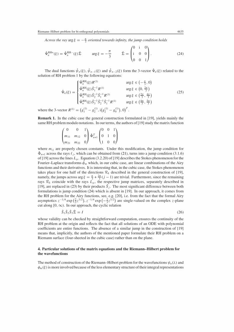
Riemann–Hilbert problem for bi-orthogonal polynomials 4635

Across the ray arg ξ = −π3 oriented towards infinity, the jump condition holds

�RH+n (ξ) = �RH−

n (ξ)� arg ξ = −π3

� =

0 i 0

i 0 0

0 0 1

. (24)

The dual functions ψn(ξ), ψn−1(ξ) and ψn−2(ξ) form the 3-vector �n(ξ) related to thesolution of RH problem 1 by the following equations:

�n(ξ) =

�RHn (ξ)R(1) arg ξ ∈ (− π

3 , 0)

�RHn (ξ)S−1

1 R(1) arg ξ ∈ (0, 2π

3

)�RHn (ξ)S−1

2 S−11 R(1) arg ξ ∈ (

2π3 ,

4π3

)�RHn (ξ)S−1

3 S−12 S−1

1 R(1) arg ξ ∈ (4π3 ,

5π3

)(25)

where the 3-vector R(1) = (g(1)1 − g

(1)2 , i

(g(1)2 − g

(1)0

), 0

)T.

Remark 1. In the cubic case the general construction formulated in [19], yields mainly thesame RH problem modulo notations. In our terms, the authors of [19] study the matrix function

0 0 1

m11 m12 0

m21 m22 0

�T

n+1

0 0 1

0 1 0

1 0 0

where mij are properly chosen constants. Under this modification, the jump condition for�n+1 across the rays �j , which can be obtained from (21), turns into a jump condition (3.1.6)of [19] across the linesLµ. Equation (3.2.20) of [19] describes the Stokes phenomenon for theFourier–Laplace transforms φm which, in our cubic case, are linear combinations of the Airyfunctions and their derivatives. It is interesting that, in the cubic case, the Stokes phenomenontakes place for one half of the directions Rk described in the general construction of [19],namely, the jumps across arg ξ = π

3 + 2π3 (j − 1) are trivial. Furthermore, since the remaining

rays Rk coincide with the rays Lµ, the respective jump matrices, separately described in[19], are replaced in (23) by their products Sj . The most significant difference between bothformulations is jump condition (24) which is absent in [19]. In our approach, it comes fromthe RH problem for the Airy functions, see, e.g. [20], i.e. from the fact that the formal Airyasymptotics z−1/4 exp

(23z

3/2), z−1/4 exp

(− 23z

3/2)

are single-valued on the complex z-planecut along [0,∞). In our approach, the cyclic relation

S1S2S3� = I (26)

whose validity can be checked by straightforward computation, ensures the continuity of theRH problem at the origin and reflects the fact that all solutions of an ODE with polynomialcoefficients are entire functions. The absence of a similar jump in the construction of [19]means that, implicitly, the authors of the mentioned paper formulate their RH problem on aRiemann surface (four-sheeted in the cubic case) rather than on the plane.

4. Particular solutions of the matrix equations and the Riemann–Hilbert problem forthe wavefunctions

The method of construction of the Riemann–Hilbert problem for the wavefunctionsψn(λ) andφm(ξ) is more involved because of the less elementary structure of their integral representations

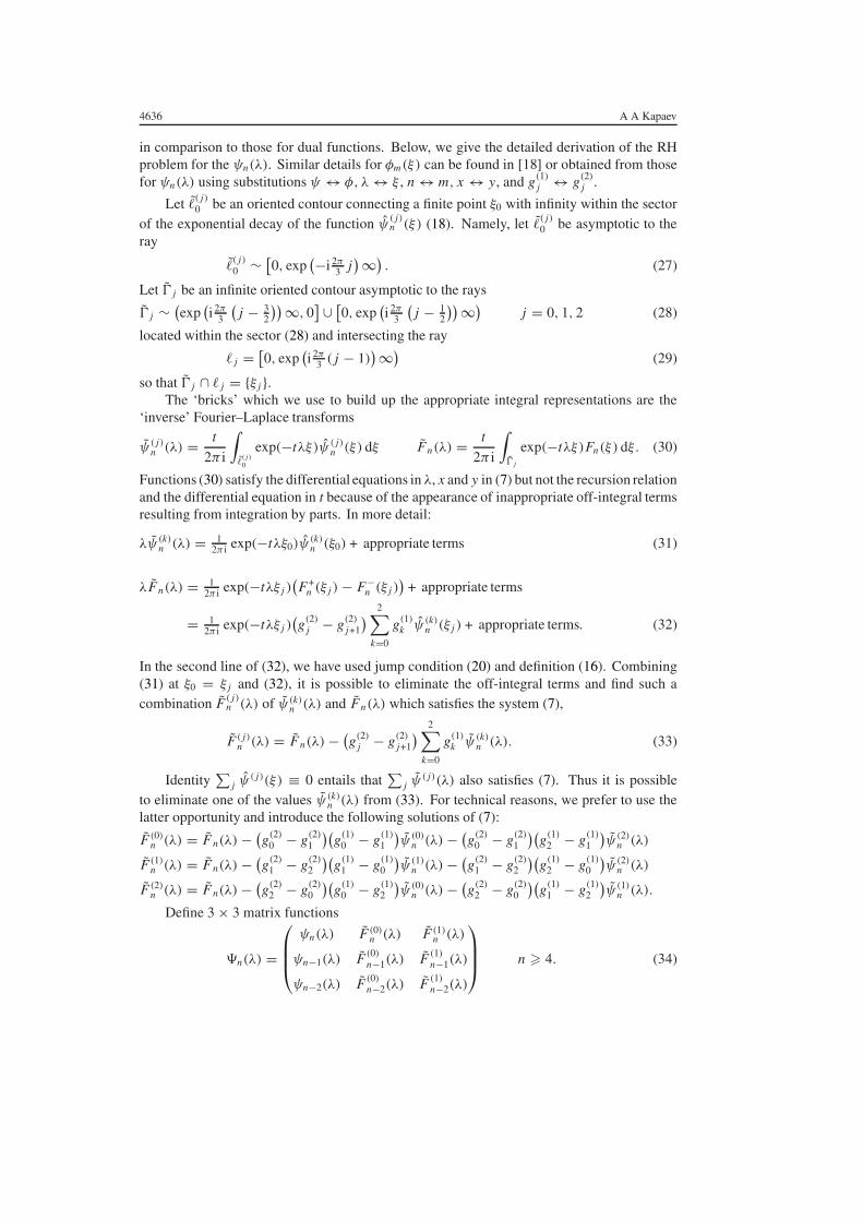
4636 A A Kapaev

in comparison to those for dual functions. Below, we give the detailed derivation of the RHproblem for the ψn(λ). Similar details for φm(ξ) can be found in [18] or obtained from thosefor ψn(λ) using substitutions ψ ↔ φ, λ ↔ ξ , n ↔ m, x ↔ y, and g(1)j ↔ g

(2)j .

Let �(j)0 be an oriented contour connecting a finite point ξ0 with infinity within the sectorof the exponential decay of the function ψ(j)

n (ξ) (18). Namely, let �(j)0 be asymptotic to theray

�(j)

0 ∼ [0, exp

(−i 2π3 j

)∞). (27)

Let �j be an infinite oriented contour asymptotic to the rays

�j ∼ (exp

(i 2π

3

(j − 3

2

))∞, 0] ∪ [

0, exp(i 2π

3

(j − 1

2

))∞)j = 0, 1, 2 (28)

located within the sector (28) and intersecting the ray

�j = [0, exp

(i 2π

3 (j − 1))∞)

(29)

so that �j ∩ �j = {ξj }.The ‘bricks’ which we use to build up the appropriate integral representations are the

‘inverse’ Fourier–Laplace transforms

ψ(j)n (λ) = t

2π i

∫�(j )

0

exp(−tλξ)ψ (j)n (ξ) dξ F n(λ) = t

2π i

∫�j

exp(−tλξ)Fn(ξ) dξ. (30)

Functions (30) satisfy the differential equations in λ, x and y in (7) but not the recursion relationand the differential equation in t because of the appearance of inappropriate off-integral termsresulting from integration by parts. In more detail:

λψ(k)n (λ) = 1

2π i exp(−tλξ0)ψ(k)n (ξ0) + appropriate terms (31)

λF n(λ) = 12π i exp(−tλξj )

(F +n (ξj )− F−

n (ξj ))

+ appropriate terms

= 12π i exp(−tλξj )

(g(2)j − g

(2)j+1

) 2∑k=0

g(1)k ψ

(k)n (ξj ) + appropriate terms. (32)

In the second line of (32), we have used jump condition (20) and definition (16). Combining(31) at ξ0 = ξj and (32), it is possible to eliminate the off-integral terms and find such acombination F (j)n (λ) of ψ(k)

n (λ) and F n(λ) which satisfies the system (7),

F (j)n (λ) = F n(λ)− (g(2)j − g

(2)j+1

) 2∑k=0

g(1)k ψ

(k)n (λ). (33)

Identity∑

j ψ(j)(ξ) ≡ 0 entails that

∑j ψ

(j)(λ) also satisfies (7). Thus it is possibleto eliminate one of the values ψ(k)

n (λ) from (33). For technical reasons, we prefer to use thelatter opportunity and introduce the following solutions of (7):

F (0)n (λ) = F n(λ)− (g(2)0 − g

(2)1

)(g(1)0 − g

(1)1

)ψ(0)n (λ)− (

g(2)0 − g

(2)1

)(g(1)2 − g

(1)1

)ψ(2)n (λ)

F (1)n (λ) = F n(λ)− (g(2)1 − g

(2)2

)(g(1)1 − g

(1)0

)ψ(1)n (λ)− (

g(2)1 − g

(2)2

)(g(1)2 − g

(1)0

)ψ(2)n (λ)

F (2)n (λ) = F n(λ)− (g(2)2 − g

(2)0

)(g(1)0 − g

(1)2

)ψ(0)n (λ)− (

g(2)2 − g

(2)0

)(g(1)1 − g

(1)2

)ψ(1)n (λ).

Define 3 × 3 matrix functions

�n(λ) =

ψn(λ) F (0)n (λ) F (1)n (λ)

ψn−1(λ) F(0)n−1(λ) F

(1)n−1(λ)

ψn−2(λ) F(0)n−2(λ) F

(1)n−2(λ)

n � 4. (34)

Riemann–Hilbert problem for bi-orthogonal polynomials 4637

The asymptotics at infinity of ψn(λ) is elementary

ψn(λ) = λn

hnexp

(− 13λ

3 − xλ)(1 + O(λ−1)). (35)

The asymptotics of F (j)n (λ) can be found using the conventional steepest descent method

F (1)n (λ) = ithn4π3/2

(tλ)−n+1

2 − 14 exp

(− 23 (tλ)

3/2 + y(tλ)1/2)(1 + O(λ−1/2)) +

(g(2)1 − g

(2)2

)

× (g(1)1 − g

(1)0

)λnhn

exp(− 1

3λ3 − xλ

)(1 + O(λ−1)) argλ ∈ (− 2π

3 , 0)

F (1)n (λ) = ithn4π3/2

(tλ)−n+1

2 − 14 exp

(− 23 (tλ)

3/2 + y(tλ)1/2)(1 + O(λ−1/2)) +

(g(2)1 − g

(2)2

)

× (g(1)2 − g

(1)0

)λnhn

exp(− 1

3λ3 − xλ

)(1 + O(λ−1)) argλ ∈ (

0, 2π3

)

F (0)n (λ) = − thn

4π3/2(−1)n(tλ)−

n+12 − 1

4 exp(

23 (tλ)

3/2 − y(tλ)1/2)(1 + O(λ−1/2)) +

(g(2)0 − g

(2)1

)

× (g(1)2 − g

(1)1

)λnhn

exp(− 1

3λ3 − xλ

)(1 + O(λ−1)) argλ ∈ (

0, 2π3

)

F (0)n (λ) = − thn

4π3/2(−1)n(tλ)−

n+12 − 1

4 exp(

23 (tλ)

3/2 − y(tλ)1/2)(1 + O(λ−1/2)) +

(g(2)0 − g

(2)1

)

× (g(1)0 − g

(1)1

)λnhn

exp(− 1

3λ3 − xλ

)(1 + O(λ−1)) argλ ∈ (

2π3 ,

4π3

)

F (2)n (λ) = − ithn4π3/2

(tλ)−n+1

2 − 14 exp

(− 23 (tλ)

3/2 + y(tλ)1/2)(1 + O(λ−1/2)) +

(g(2)2 − g

(2)0

)

× (g(1)0 − g

(1)2

)λnhn

exp(− 1

3λ3 − xλ

)(1 + O(λ−1)) argλ ∈ (

2π3 ,

4π3

)

F (2)n (λ) = − ithn2π3/2

(tλ)−n+1

2 − 14 exp

(− 23 (tλ)

3/2 + y(tλ)1/2)(1 + O(λ−1/2)) +

(g(2)2 − g

(2)0

)

× (g(1)1 − g

(1)2

)λnhn

exp(− 1

3λ3 − xλ

)(1 + O(λ−1)) argλ ∈ (

4π3 , 2π

).

Using the above asymptotics and the linear constraint for F (j)n ,

F (0)n (λ) + F (1)n (λ) + F (2)n (λ) = gFψn(λ)

gF = g(2)0

(g(1)2 − g

(1)1

)+ g(2)1

(g(1)1 − g

(1)0

)+ g(2)2

(g(1)0 − g

(1)2

)(36)

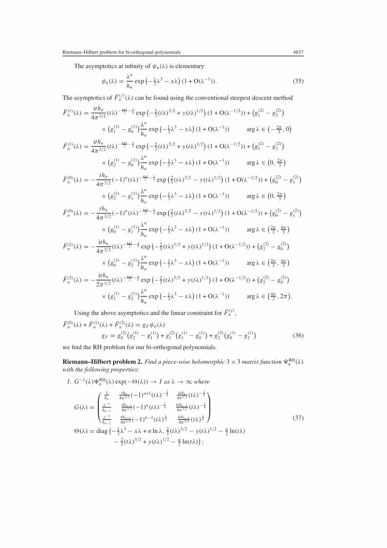
we find the RH problem for our bi-orthogonal polynomials.

Riemann–Hilbert problem 2. Find a piece-wise holomorphic 3 × 3 matrix function�RHn (λ)

with the following properties:

1. G−1(λ)�RHn (λ) exp(−�(λ)) → I as λ → ∞ where

G(λ) =

1hn

thn4π3/2 (−1)n+1(tλ)−

34

ithn4π3/2 (tλ)

− 34

λ−1

hn−1

thn−1

4π3/2 (−1)n(tλ)−14

ithn−1

4π3/2 (tλ)− 1

4

λ−2

hn−2

thn−2

4π3/2 (−1)n−1(tλ)14

ithn−2

4π3/2 (tλ)14

�(λ) = diag(− 1

3λ3 − xλ + n ln λ, 2

3 (tλ)3/2 − y(tλ)1/2 − n

2 ln(tλ)

− 23 (tλ)

3/2 + y(tλ)1/2 − n2 ln(tλ)

) ;

(37)

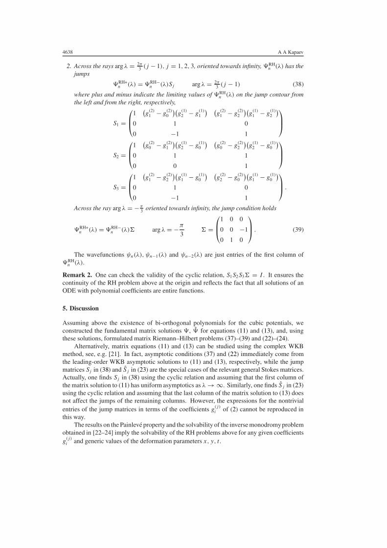
4638 A A Kapaev

2. Across the rays argλ = 2π3 (j − 1), j = 1, 2, 3, oriented towards infinity, �RH

n (λ) has thejumps

�RH+n (λ) = �RH−

n (λ)Sj argλ = 2π3 (j − 1) (38)

where plus and minus indicate the limiting values of �RHn (λ) on the jump contour from

the left and from the right, respectively,

S1 =

1(g(2)1 − g

(2)0

)(g(1)2 − g

(1)1

) (g(2)1 − g

(2)2

)(g(1)1 − g

(1)2

)0 1 0

0 −1 1

S2 =

1(g(2)0 − g

(2)1

)(g(1)2 − g

(1)0

) (g(2)0 − g

(2)2

)(g(1)2 − g

(1)0

)0 1 1

0 0 1

S3 =

1(g(2)1 − g

(2)2

)(g(1)1 − g

(1)0

) (g(2)2 − g

(2)0

)(g(1)1 − g

(1)0

)0 1 0

0 −1 1

.

Across the ray argλ = −π3 oriented towards infinity, the jump condition holds

�RH+n (λ) = �RH−

n (λ)� argλ = −π3

� =

1 0 0

0 0 −1

0 1 0

. (39)

The wavefunctions ψn(λ),ψn−1(λ) and ψn−2(λ) are just entries of the first column of�RHn (λ).

Remark 2. One can check the validity of the cyclic relation, S1S2S3� = I . It ensures thecontinuity of the RH problem above at the origin and reflects the fact that all solutions of anODE with polynomial coefficients are entire functions.

5. Discussion

Assuming above the existence of bi-orthogonal polynomials for the cubic potentials, weconstructed the fundamental matrix solutions � , � for equations (11) and (13), and, usingthese solutions, formulated matrix Riemann–Hilbert problems (37)–(39) and (22)–(24).

Alternatively, matrix equations (11) and (13) can be studied using the complex WKBmethod, see, e.g. [21]. In fact, asymptotic conditions (37) and (22) immediately come fromthe leading-order WKB asymptotic solutions to (11) and (13), respectively, while the jumpmatrices Sj in (38) and Sj in (23) are the special cases of the relevant general Stokes matrices.Actually, one finds Sj in (38) using the cyclic relation and assuming that the first column ofthe matrix solution to (11) has uniform asymptotics as λ → ∞. Similarly, one finds Sj in (23)using the cyclic relation and assuming that the last column of the matrix solution to (13) doesnot affect the jumps of the remaining columns. However, the expressions for the nontrivialentries of the jump matrices in terms of the coefficients g(j)i of (2) cannot be reproduced inthis way.

The results on the Painleve property and the solvability of the inverse monodromy problemobtained in [22–24] imply the solvability of the RH problems above for any given coefficientsg(j)

i and generic values of the deformation parameters x, y, t .

Riemann–Hilbert problem for bi-orthogonal polynomials 4639

Uniqueness of these solutions can be obtained in the usual way. For instance, considerRH problem 2. Introduce the matrix function Y = G−1�RH e−�. It is straightforward thatdetY is an entire function of λ. Moreover, det Y ≡ 1 due to the Liouville theorem andnormalization (37). Consider two solutions�RH and �RH of RH problem 2 and the respectivefunctions Y and Y . The ratio Z = Y Y−1 is an entire function of λ, moreoverZ ≡ I due to theLiouville theorem and normalization (37). Thus �RH ≡ �RH. Uniqueness of the solution toRH problem 1 is similar.

The above discussion of the unique solvability of the RH problems is independent fromthe fact of existence of the bi-orthogonal polynomials assumed in sections 3 and 4. Following[19] and using a determinant representation for the bi-orthogonal polynomials, it is possibleto justify this assumption for arbitrary values of the deformation parameters x, y, t and somegeneric values of g(j)i .

We observe another opportunity to make sure that the set of bi-orthogonal polynomials forany g(j)i and generic x, y, t is not empty. Namely, we conjecture that the solvability of the RHproblems for�RH, �RH,�RH, �RH leads to the existence of bi-orthogonal polynomials. Thisassertion can be obtained as follows. The solution �RH(λ) of RH problem 2 contains in itsfirst column a polynomial vector. The solution �RH(ξ) of RH problem 1 gives rise to a matrixfunction �(ξ) with the jump property (21). Thus the first two columns of �(ξ) are entirefunctions, while the last column admits a Cauchy integral representation. Then the prescribedasymptotics at infinity of the latter yields the orthogonality of a combination of the first twocolumns to ξm exp(−W(ξ)) form < n. To complete the proof it is enough to observe that thefirst two columns of �(ξ) are just Fourier–Laplace transforms of the first column in �RH(λ).

Finally, we note that the RH problems constructed above are useful for the study ofn-large asymptotics of the bi-orthogonal polynomials. The necessary preparatory steps andanticipated results are announced in [25].

Acknowledgments

This work was partially supported by the EPSRC and the RFBR (grant no 02-01-00268). Theauthor thanks J Harnad and M Bertola for stimulating discussions and valuable comments.The author is also grateful to A S Fokas for support and to the staff of DAMTP, University ofCambridge, for the hospitality during his visit.

References

[1] Plancherel M and Rotach W 1929 Sur les valeurs asymptotiques des poynomes d’Hermite Hn(x) =(−1)nex

2/2dn(e−x2/2)/dxn Comment. Math. Helv. 1 227–54[2] Szego G 1939 Orthogonal Polynomials (Providence, RI: American Mathematical Society)[3] Freud G 1976 On the coefficients in the recursion formulae of orthogonal polynomials Proc. R. Ir. Acad. A 76

1–6[4] Nevai P 1986 Geza Freud, orthogonal polynomials and Christoffel functions. A case study J. Approx. Theory

48 3–167[5] Sheen R -C 1987 Plancherel–Rotach-type asymptotics for orthogonal polynomials associated with exp(−x6/6)

J. Approx. Theory 50 232–93[6] Magnus A P 1995 Painleve-type differential equations for the recurrence coefficients of semi-classical orthogonal

polynomials J. Comput. Appl. Math. 57 215–37[7] Fokas A S, Its A R and Kitaev A V 1990 Isomonodromic approach in the theory of two-dimensional quantum

gravity Usp. Mat. Nauk 45 135–6Fokas A S, Its A R and Kitaev A V 1991 Discrete Painleve equations and their appearance in quantum gravity

Comment Math. Phys. 142 313–44

4640 A A Kapaev

Fokas A S, Its A R and Kitaev A V 1992 The isomonodromy approach to matrix models in 2D quantum gravityCommun. Math. Phys. 147 395–430

[8] Deift P A and Zhou X 1993 A steepest descent method for oscillatory Riemann–Hilbert problems. Asymptoticsfor the MKdV equation Ann. Math. 137 295–368

[9] Bleher P M and Its A R 1999 Semiclassical asymptotics of orthogonal polynomials, Riemann–Hilbert problem,and universality in the matrix model Ann. Math. 150 185–266

Bleher P M and Its A R 2002 Double scaling limit in the random matrix model: Riemann–Hilbert approachPreprint math-ph/0201003

[10] Deift P, Kriecherbauer T, McLaughlin K T-R, Venakides S and Zhou X 1999 Uniform asymptotics forpolynomials orthogonal with respect to varying exponential weights and applications to universality questionsin random matrix theory Commun. Pure Appl. Math. 52 1335–425

Deift P, Kriecherbauer T, McLaughlin K T-R, Venakides S and Zhou X 1999 Strong asymptotics of orthogonalpolynomials with respect to exponential weights Commun. Pure Appl. Math. 52 1491–552

[11] Baik J, Deift P and Johansson K 1999 On the distribution of the length of the longest increasing subsequenceof random permutations J. Am. Math. Soc. 12 1119–78 (Preprint math.CO/9810105)

[12] Adler M and van Moerbeke P 2000 Generalized orthogonal polynomials, discrete KP and Riemann–Hilbertproblems Preprint nlin.SI/0009002

[13] van Moerbeke P 2001 Integrable Lattices: Random Matrices and Random Permutations (MSRI PublicationsNo 40) (Cambridge: Cambridge University Press) (Preprint math.CO/0010135)

[14] Ercolani N M and McLaughlin K T-R 2001 Asymptotics and integrable structures for biorthogonal polynomialsassociated to a random two-matrix model Physica D 152–153 232–68

[15] Bertola M, Eynard B and Harnad J 2001 Duality, biorthogonal polynomials and multi-matrix models Preprintnlin.SI/0108049

[16] Zinn-Justin P 2002 HCIZ integral and 2D Toda lattice hierarchy Preprint math-ph/0202045[17] Bertola M 2002 Bilinear semi-classical moment functionals and their integral representation Preprint

math.CA/0205160[18] Kapaev A A 2002 The Riemann–Hilbert problem for the bi-orthogonal polynomials Preprint nlin.SI/0207036[19] Bertola M, Eynard B and Harnad J 2002 Differential systems appearing in 2-matrix models and the associated

Riemann–Hilbert problem Preprint nlin.SI/0208002[20] Its A R and Kapaev A A 2002 The nonlinear steepest descent approach to the asymptotics of the second Painleve

transcendent in the complex domain MathPhys Odyssey 2001, Integrable Models and Beyond (in Honour ofBarry M McCoy) ed M Kashiwara and T Miwa (Progress in Mathematical Physics vol 23) (Boston, MA:Birkhauser) pp 273–311 (Preprint nlin.SI/0108054)

[21] Wasow W 1965 Asymptotic Expansions for Ordinary Differential Equations (New York: Interscience/Wiley)[22] Miwa T 1981 Painleve property of monodromy preserving equations and the analyticity of τ -functions Publ.

Res. Inst. Math. Sci. 17 703–21[23] Malgrange B 1991 Differential Equations with Polynomial Coefficients (Progress in Mathematics vol 96)

(Boston, MA: Birkhauser)[24] Bolibrukh A, Its A R and Kapaev A A On the Riemann–Hilbert–Birkhoff inverse monodromy problem and the

Painleve equations In preparation[25] Kapaev A A 2002 Monodromy approach to the scaling limits in the isomonodromy systems Preprint

nlin.SI/0211022