Embed Size (px)
Citation preview
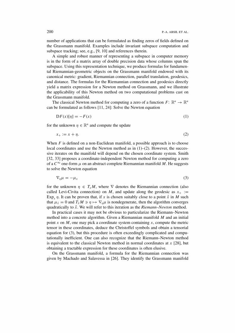
Acta Applicandae Mathematicae 80: 199–220, 2004.© 2004 Kluwer Academic Publishers. Printed in the Netherlands.
199
Riemannian Geometry of Grassmann Manifoldswith a View on Algorithmic Computation
P.-A. ABSIL1,�, R. MAHONY2 and R. SEPULCHRE3
1School of Computational Science and Information Technology, Florida State University,Tallahassee, FL 32306-4120, USA2Department of Engineering, Australian National University, ACT, 0200, Australia3Department of Electrical Engineering and Computer Science, Université de Liège,Bât. B28 Systèmes, Grande Traverse 10, B-4000 Liège, Belgium
(Received: 7 November 2002; in final form: 14 October 2003)
Abstract. We give simple formulas for the canonical metric, gradient, Lie derivative, Riemannianconnection, parallel translation, geodesics and distance on the Grassmann manifold of p-planes inRn. In these formulas, p-planes are represented as the column space of n× p matrices. The Newton
method on abstract Riemannian manifolds proposed by Smith is made explicit on the Grassmannmanifold. Two applications – computing an invariant subspace of a matrix and the mean of subspaces– are worked out.
Mathematics Subject Classifications (2000): 65J05, 53C05, 14M15.
Key words: Grassmann manifold, noncompact Stiefel manifold, principal fiber bundle, Levi-Civitaconnection, parallel transportation, geodesic, Newton method, invariant subspace, mean of sub-spaces.
1. Introduction
The majority of available numerical techniques for optimization and nonlinearequations assume an underlying Euclidean space. Yet many computational prob-lems are posed on non-Euclidean spaces. Several authors [16, 27, 28, 33, 35] haveproposed abstract algorithms that exploit the underlying geometry (e.g., symmet-ric, homogeneous, Riemannian) of manifolds on which problems are cast, but theconversion of these abstract geometric algorithms into numerical procedures inpractical situations is often a nontrivial task that critically relies on an adequaterepresentation of the manifold.
The present paper contributes to addressing this issue in the case, where therelevant non-Euclidean space is the set of fixed dimensional subspaces of a givenEuclidean space. This non-Euclidean space is commonly called the Grassmannmanifold. Our motivation for considering the Grassmann manifold comes from the
� Part of this work was done while the author was a Research Fellow with the Belgian NationalFund for Scientific Research (Aspirant du F.N.R.S.) at the University of Liege.
200 P.-A. ABSIL ET AL.
number of applications that can be formulated as finding zeros of fields defined onthe Grassmann manifold. Examples include invariant subspace computation andsubspace tracking; see, e.g., [9, 10] and references therein.
A simple and robust manner of representing a subspace in computer memoryis in the form of a matrix array of double precision data whose columns span thesubspace. Using this representation technique, we produce formulas for fundamen-tal Riemannian-geometric objects on the Grassmann manifold endowed with itscanonical metric: gradient, Riemannian connection, parallel translation, geodesics,and distance. The formulas for the Riemannian connection and geodesics directlyyield a matrix expression for a Newton method on Grassmann, and we illustratethe applicability of this Newton method on two computational problems cast onthe Grassmann manifold.
The classical Newton method for computing a zero of a function F : Rn → R
n
can be formulated as follows [11, 24]: Solve the Newton equation
DF(x)[η] = −F(x) (1)
for the unknown η ∈ Rn and compute the update
x+ := x + η. (2)
When F is defined on a non-Euclidean manifold, a possible approach is to chooselocal coordinates and use the Newton method as in (1)–(2). However, the succes-sive iterates on the manifold will depend on the chosen coordinate system. Smith[32, 33] proposes a coordinate-independent Newton method for computing a zeroof aC∞ one-form µ on an abstract complete Riemannian manifoldM. He suggeststo solve the Newton equation
∇ηµ = −µx (3)
for the unknown η ∈ TxM, where ∇ denotes the Riemannian connection (alsocalled Levi-Civita connection) on M, and update along the geodesic as x+ :=Expx η. It can be proven that, if x is chosen suitably close to a point x in M suchthat µx = 0 and TxM η �→ ∇ηµ is nondegenerate, then the algorithm convergesquadratically to x. We will refer to this iteration as the Riemann–Newton method.
In practical cases it may not be obvious to particularize the Riemann–Newtonmethod into a concrete algorithm. Given a Riemannian manifold M and an initialpoint x onM, one may pick a coordinate system containing x, compute the metrictensor in these coordinates, deduce the Christoffel symbols and obtain a tensorialequation for (3), but this procedure is often exceedingly complicated and compu-tationally inefficient. One can also recognize that the Riemann–Newton methodis equivalent to the classical Newton method in normal coordinates at x [28], butobtaining a tractable expression for these coordinates is often elusive.
On the Grassmann manifold, a formula for the Riemannian connection wasgiven by Machado and Salavessa in [26]. They identify the Grassmann manifold
RIEMANNIAN GEOMETRY OF GRASSMANN MANIFOLDS 201
with the set of projectors into subspaces of Rn, embed the set of projectors in the
set of linear maps from Rn to R
n (which is an Euclidean space), and endow thisset with the Hilbert–Schmidt inner product. The induced metric on the Grassmannmanifold is then the essentially unique On-invariant metric mentioned above. Theembedding of the Grassmann manifold in an Euclidean space allows the authorsto compute the Riemannian connection by taking the derivative in the Euclideanspace and projecting the result into the tangent space of the embedded manifold.They obtain a formula for the Riemannian connection in terms of projectors.
Edelman, Arias and Smith [14] have proposed an expression of the Riemann–Newton method on the Grassmann manifold in the particular case where µ is thedifferential df of a real function f on M. Their approach avoids the derivationof a formula for the Riemannian connection on Grassmann. Instead, they obtain aformula for the Hessian (∇�1df )�2 by polarizing the second derivative of f alongthe geodesics.
In the present paper, we derive an easy-to-use formula for the Riemannian con-nection ∇ηξ where η and ξ are arbitrary smooth vector fields on the Grassmannmanifold of p-dimensional subspaces of R
n. This formula, expressed in terms ofn × p matrices, intuitively relates to the geometry of the Grassmann manifoldexpressed as a set of equivalence classes of n × p matrices. Once the formula forRiemannian connection is available, expressions for parallel transport and geodes-ics follow directly. Expressing the Riemann–Newton method on the Grassmannmanifold for concrete vector fields ξ reduces to a directional derivative in R
n
followed by a projection.We work out an example where the zeros of ξ are the p-dimensional right-
invariant subspaces of an arbitrary n× n matrix A. This generalizes an applicationconsidered in [14] where ξ was the gradient of a generalized scalar Rayleighquotient of a matrix A = AT. The Newton method for our ξ converges locallyquadratically to the nondegenerate zeros of ξ . We show that the rate of convergenceis cubic if and only if the targeted zero of ξ is also a left-invariant subspace of A.In a second example, the zero of ξ is the mean of a collection of p-dimensionalsubspaces of R
n. We illustrate by a numerical experiment the fast convergence ofthe Newton algorithm to the mean subspace.
The present paper only requires from the reader an elementary backgroundin Riemannian geometry (tangent vectors, gradient, parallel transport, geodesics,distance), which can be read, e.g., from Boothby [6], do Carmo [12] or the introduc-tory chapter of [8]. The relevant definitions are summarily recalled in the text. Con-cepts of reductive homogeneous space and symmetric spaces (see [6, 18, 22, 29]and particularly Sections II.4, IV.3, IV.A and X.2 in the latter) are not needed, butthey can help to get insight into the problem. Although some elementary conceptsof principal fiber bundle theory [22] are used, no specific background is needed.
The paper is organized as follows. In Section 2, the linear subspaces of Rn
are identified with equivalent classes of matrices and the manifold structure ofGrassmann is defined. Section 3 defines a Riemannian structure on Grassmann.
202 P.-A. ABSIL ET AL.
Formulas are given for Lie brackets, Riemannian connection, parallel transport,geodesics, and distance between subspaces. The Grassmann–Newton algorithm ismade explicit in Section 4 and practical applications are worked out in detail inSection 5.
2. The Grassmann Manifold
The goal of this section is to recall relevant facts about the Grassmann manifolds.More details can be read from [6, 13, 15, 19, 36].
Let n be a positive integer and let p be a positive integer not greater than n. Theset of p-dimensional linear subspaces of R
n (‘linear’ will be omitted in the sequel)is termed the Grassmann manifold, denoted here by Grass(p, n).
An element Y of Grass(p, n), i.e., a p-dimensional subspace of Rn, can be
specified by a basis, i.e., a set of p vectors y1, . . . , yp such that Y is the set ofall their linear combinations. If the y’s are ordered as the columns of an n-by-pmatrix Y , then Y is said to span Y and Y is said to be the column space (or range,or image, or span) of Y , and we write Y = span(Y ). The span of an n-by-p matrixY is an element of Grass(p, n) if and only if Y has a full rank. The set of suchmatrices is termed the noncompact Stiefel manifold�
ST(p, n) := {Y ∈ Rn×p : rank(Y ) = p}.
Given Y ∈ Grass(p, n), the choice of a Y in ST(p, n) such that Y spans Y isnot unique. There are infinitely many possibilities. Given a matrix Y in ST(p, n),the set of the matrices in ST(p, n) that have the same span as Y is
YGLp := {YM : M ∈ GLp}, (4)
where GLp denotes the set of the p-by-p invertible matrices. This identifiesGrass(p, n) with the quotient space ST(p, n)/GLp := {YGLp : Y ∈ ST(p, n)}. Infiber bundle theory, the quadruple (GLp,ST(p, n), π,Grass(p, n)) is called a prin-cipal GLp fiber bundle, with the total space ST(p, n), base space Grass(p, n) =ST(p, n)/GLp, group action
ST(p, n)× GLp (Y,M) �→ YM ∈ ST(p, n)
and projection map
π : ST(p, n) Y �→ span(Y ) ∈ Grass(p, n).
See, e.g., [22] for the general theory of principal fiber bundles and [15] for a de-tailed treatment of the Grassmann case. In this paper, we use the notation span(Y )and π(Y ) to denote the column space of Y .
To each subspace Y corresponds an equivalence class (4) of n-by-p matricesthat span Y, and each equivalence class contains infinitely many elements. It is� The (compact) Stiefel manifold is the set of orthonormal n× p matrices.
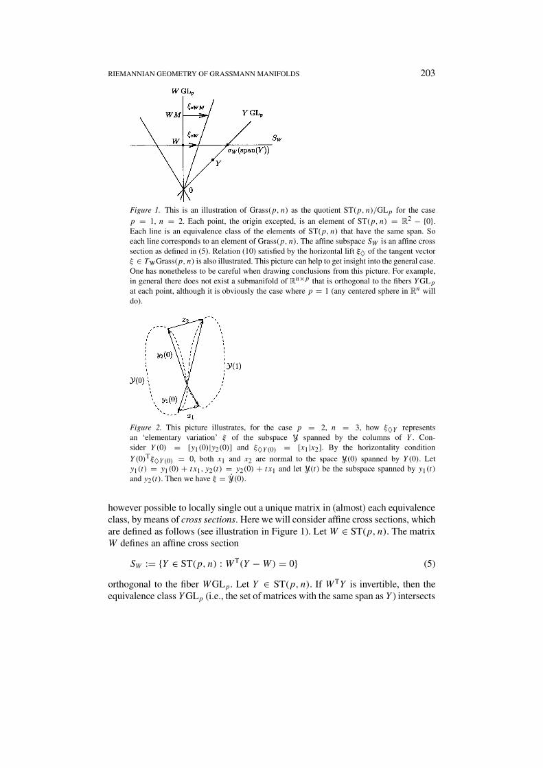
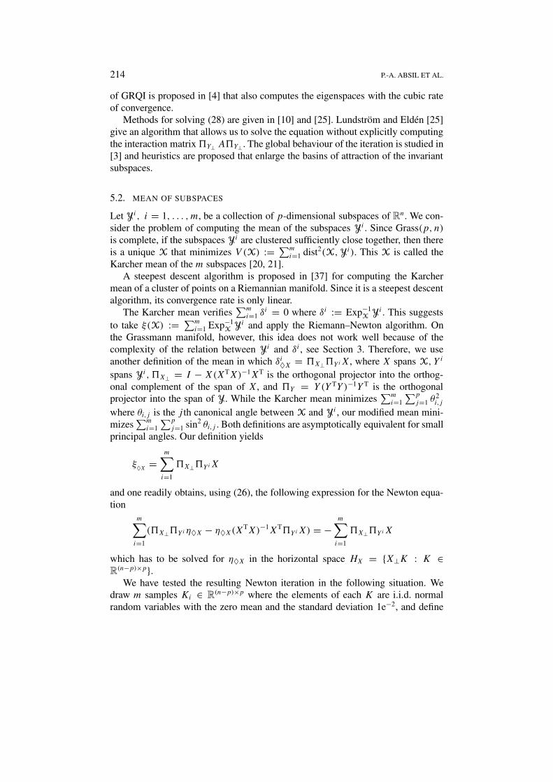
RIEMANNIAN GEOMETRY OF GRASSMANN MANIFOLDS 203
Figure 1. This is an illustration of Grass(p, n) as the quotient ST(p, n)/GLp for the casep = 1, n = 2. Each point, the origin excepted, is an element of ST(p, n) = R
2 − {0}.Each line is an equivalence class of the elements of ST(p, n) that have the same span. Soeach line corresponds to an element of Grass(p, n). The affine subspace SW is an affine crosssection as defined in (5). Relation (10) satisfied by the horizontal lift ξ♦ of the tangent vectorξ ∈ TW Grass(p, n) is also illustrated. This picture can help to get insight into the general case.One has nonetheless to be careful when drawing conclusions from this picture. For example,in general there does not exist a submanifold of R
n×p that is orthogonal to the fibers YGLpat each point, although it is obviously the case where p = 1 (any centered sphere in R
n willdo).
Figure 2. This picture illustrates, for the case p = 2, n = 3, how ξ♦Y representsan ‘elementary variation’ ξ of the subspace Y spanned by the columns of Y . Con-sider Y(0) = [y1(0)|y2(0)] and ξ♦Y (0) = [x1|x2]. By the horizontality conditionY(0)Tξ♦Y (0) = 0, both x1 and x2 are normal to the space Y(0) spanned by Y(0). Lety1(t) = y1(0) + tx1, y2(t) = y2(0) + tx1 and let Y(t) be the subspace spanned by y1(t)
and y2(t). Then we have ξ = Y(0).
however possible to locally single out a unique matrix in (almost) each equivalenceclass, by means of cross sections. Here we will consider affine cross sections, whichare defined as follows (see illustration in Figure 1). LetW ∈ ST(p, n). The matrixW defines an affine cross section
SW := {Y ∈ ST(p, n) : WT(Y −W) = 0} (5)
orthogonal to the fiber WGLp. Let Y ∈ ST(p, n). If WTY is invertible, then theequivalence class YGLp (i.e., the set of matrices with the same span as Y ) intersects
204 P.-A. ABSIL ET AL.
the cross section SW at the single point Y (WTY )−1WTW . IfWTY is not invertible,which means that the span of W contains an orthogonal direction to the span of Y ,then the intersection between the fiber WGLp and the section SW is empty. Let
UW := {span(Y ) : WTY is invertible} (6)
be the set of subspaces whose representing fiber YGLp intersects the section SWThe mapping
σW : UW span(Y ) �→ Y (WTY )−1WTW ∈ SW, (7)
which we will call cross section mapping, realizes a bijection between the subsetUW of Grass(p, n) and the affine subspace SW of ST(p, n). The classical manifoldstructure of Grass(p, n) is the one that, for all W ∈ ST(p, n), makes σW a dif-feomorphism between UW and SW (embedded in the Euclidean space R
n×p) [15].Parameterizations of Grass(p, n) are then given by
R(n−p)×p K �→ π(W +W⊥K) = span(W +W⊥K) ∈ UW ,
where W⊥ is any element of ST(n− p, n) such that WTW⊥ = 0.
3. Riemannian Structure on Grass(p, n) = ST(p, n)/GLp
The goal of this section is to define a Riemannian metric on Grass(p, n) and thenderive formulas for the associated gradient, connection, and geodesics. For an in-troduction to Riemannian geometry, see, e.g., [6, 12], or the introductory chapterof [8].
3.1. TANGENT VECTORS
A tangent vector ξ to Grass(p, n) at W can be thought of as an elementary variationof the p-dimensional subspace W (see [6, 12] for a more formal definition of atangent vector). Here we give a way to represent ξ by a matrix. The principle is todecompose variations of a basisW of W into a component that does not modify thespan, and a component that does modify the span. The latter represents a tangentvector of Grass(p, n) at W .
LetW ∈ ST(p, n). The tangent space to ST(p, n) atW , denoted as TWST(p, n),is trivial: ST(p, n) is an open subset of R
n×p, so ST(p, n) and Rn×p are identical
in a neighbourhood of W , and therefore TWST(p, n) = TWRn×p which is just a
copy of Rn×p . The vertical space VW is by definition the tangent space to the fiber
WGLp, namely,
VW = WRp×p = {Wm : m ∈ R
p×p}.Its elements are the elementary variations of W that do not modify its span. Wedefine the horizontal space HW as
HW := TWSW = {W⊥K : K ∈ R(n−p)×p}. (8)
RIEMANNIAN GEOMETRY OF GRASSMANN MANIFOLDS 205
One readily verifies that HW verifies the characteristic properties of horizontalspaces in principal fiber bundles [15, 22]. In particular, TWST(p, n) = VW ⊕ HW .Note that with our choice of HW,�T
V�H = 0 for all �V ∈ VW and �H ∈ HW .Let ξ be a tangent vector to Grass(p, n) at W and let W span W . According to
the theory of principal fiber bundles [22], there exists one and only one horizontalvector ξ♦W that represents ξ in the sense that ξ♦W projects to ξ via the span opera-tion, i.e., dπ(W)ξ♦W = ξ . See Figure 1 for a graphical interpretation. It is easy tocheck that
ξ♦W = dσW(W)ξ, (9)
where σW is the cross section mapping defined in (7). Indeed, it is horizontal andprojects to ξ via π since π ◦ σW is locally the identity. The representation ξ♦Wis called the horizontal lift of ξ ∈ TW Grass(p, n) at W . The next propositioncharacterizes how the horizontal lift varies along the equivalence class WGLp.
PROPOSITION 3.1. Let W ∈ Grass(p, n), letW span W and ξ ∈ TW Grass(p, n).Let ξ♦W denote the horizontal lift of ξ at W . Then for allM ∈ GLp,
ξ♦WM = ξ♦WM. (10)
Proof. This comes from (9) and the property σWM(Y) = σW(Y)M. ✷The homogeneity property (10) and the horizontally of ξ♦W are characteristic
of horizontal lifts.We now introduce notation for derivatives. Let f be a smooth function between
two linear spaces. We denote by
Df (x)[y] := d
dtf (x + ty) |t=0
the directional derivative of f at x in the direction of y. Let f be a smooth real-valued function defined on Grass(p, n) in a neighbourhood of W . We will use thenotation f♦(W) to denote f (span(W)). The derivative of f in the direction of thetangent vector ξ at W , denoted by ξf , can be computed as
ξf = Df♦(W)[ξ♦W ],where W spans W .
3.2. LIE DERIVATIVE
A tangent vector field ξ on Grass(p, n) assigns to each Y ∈ Grass(p, n) an elementξY ∈ TYGrass(p, n).
206 P.-A. ABSIL ET AL.
PROPOSITION 3.2 (Lie bracket). Let η and ξ be smooth tangent vector fields onGrass(p, n). Let ξ♦W denote the horizontal lift of ξ at W as defined in (9). Then
[η, ξ ]♦W = W⊥[η♦W , ξ♦W ], (11)
where
W⊥ := I −W(WTW)−1WT (12)
denotes the projection into the orthogonal complement of the span of W and
[η♦W , ξ♦W ] = Dξ♦·(W)[η♦W ] − Dη♦·(W)[η♦W ]denotes the Lie bracket in R
n×p.
That is, the horizontal lift of the Lie bracket of two tangent vector fields onthe Grassmann manifold is equal to the horizontal projection of the Lie bracket ofhorizontal lifts of the two tangent vector fields.
Proof. Let W ∈ ST(p, n) be fixed. We prove formula (11) by computing in thecoordinate chart (UW, σW). In order to simplify the notation, let Y := σWY andξY := σW∗YξY. Note that W = W and ξW = ξ♦W . One has
[η, ξ ]♦W = Dξ .(W)[ηW ] − Dη.(W)[ξW ].After some manipulations using (5) and (7), it comes
ξY = d
dtσW�Y + ξ♦Y t� |t=0= ξ♦Y − Y (WTW)−1WTξ♦Y .
Then, using WTξ♦W = 0,
Dξ .(W)[ηW ] = Dξ♦·(W)[ηW ] −W(WTW)−1WTDξ♦·(W)[ηW ].The term Dη.(W)[ξW ] is directly deduced by interchanging ξ and η, and the resultis proved. ✷
3.3. METRIC
We consider the following metric on Grass(p, n):
〈ξ, η〉Y := trace((Y TY )−1ξT♦Yη♦Y ), (13)
where Y spans Y. It is easily checked that expression (13) does not depend on thechoice of the basis Y that spans Y. This metric is the only one (up to multiplicationsby a constant) to be invariant under the action of On on R
n. Indeed,
trace(((QY )TQY)−1(Qξ♦Y )TQη♦Y ) = trace((Y TY )−1ξT♦Yη♦Y )
RIEMANNIAN GEOMETRY OF GRASSMANN MANIFOLDS 207
for all Q ∈ On, and uniqueness is proved in [23]. We will see later that thedefinition (13) induces a natural notion of distance between subspaces.
3.4. GRADIENT
On an abstract Riemannian manifold M, the gradient of a smooth real function fat a point x of M, denoted by grad f (x), is roughly speaking the steepest ascentvector of f in the sense of the Riemannian metric. More rigorously, grad f (x)is the element of TxM satisfying 〈grad f (x), ξ 〉 = ξf for all ξ ∈ TxM. On theGrassmann manifold Grass(p, n) endowed with the metric (13), one checks that
(grad f )♦Y = Y⊥grad f♦(Y )Y TY, (14)
where Y⊥ is the orthogonal projection (12) into the orthogonal complement ofY, f♦(Y ) = f (span(Y )) and grad f♦(Y ) is the Euclidean gradient of f♦ at Y ,given by (grad f♦(Y ))ij = ∂f♦(Y )
∂Yij(Y ). The Euclidean gradient is characterized by
Df♦(Y )[Z] = trace(ZTgrad f♦(Y )), ∀Z ∈ Rn×p, (15)
which can ease its computation in some cases.
3.5. RIEMANNIAN CONNECTION
Let ξ, η be two tangent vector fields on Grass(p, n). There is no predefined way ofcomputing the derivative of ξ in the direction of η because there is no predefinedway of comparing the different tangent spaces TYGrass(p, n) as Y varies. However,there is a prefered definition for the directional derivative, called the Riemannianconnection (or Levi-Civita connection), defined as follows [6, 12].
DEFINITION 3.3 (Riemannian connection). LetM be a Riemannian manifold andits metric be denoted by 〈·, ·〉. Let x ∈ M. The Riemannian connection ∇ on Mhas the following properties: For all smooth real functions f, g on M, all η, η′ inTxM and all smooth vector fields ξ, ξ ′:
(1) ∇f η+gη′ξ = f∇ηξ + g∇η′ξ ,(2) ∇η(f ξ + gξ ′) = f∇ηξ + g∇ηξ ′ + (ηf )ξ + (ηg)ξ ′,(3) [ξ, ξ ′] = ∇ξ ξ ′ − ∇ξ ′ξ ,(4) η〈ξ, ξ ′〉 = 〈∇ηξ, ξ ′〉 + 〈ξ,∇ηξ ′〉.
Properties (1) and (2) define connections in general. Property (3) states thatthe connection is torsion-free, and property (4) specifies that the metric tensor isinvariant by the connection. A famous theorem of Riemannian geometry states thatthere is one and only one connection verifying these four properties. If M is asubmanifold of an Euclidean space, then the Riemannian connection ∇ηξ consistsin taking the derivative of ξ in the ambient Euclidean space in the direction of η
208 P.-A. ABSIL ET AL.
and projecting the result into the tangent space of the manifold. As we show in thenext theorem, the Riemannian connection on the Grassmann manifold, expressedin terms of horizontal lifts, works in a similar way.
THEOREM 3.4 (Riemannian connection). Let Y ∈ Grass(p, n), and Y ∈ ST(p, n)span Y. Let η ∈ TYGrass(p, n), and ξ be a smooth tangent vector field defined ina neighbourhood of Y. Let ξ♦: W �→ ξ♦W be the horizontal lift of ξ as definedin (9). Let Grass(p, n) be endowed with the On-invariant Riemannian metric (13)and let ∇ denote the associated Riemannian connection. Then
(∇ηξ)♦Y = Y⊥∇η♦Y ξ♦, (16)
where Y⊥ is the projection (12) into the orthogonal complement of Y and
∇η♦Y ξ♦ := Dξ♦·(Y )[η♦Y ] := d
dtξ♦(Y+η♦Y t)
∣∣∣∣t=0
is the directional derivative of ξ♦ in the direction of η♦Y in the Euclidean spaceRn×p.
This theorem says that the horizontal lift of the covariant derivative of a vectorfield ξ on Grassmann in the direction of η is equal to the horizontal projection of aderivative of the horizontal lift of ξ in the direction of the horizontal lift of η.
Proof. One has to prove that (16) satisfies the four characteristic properties ofthe Riemannian connection. The two first properties concern linearity in η and ξand are easily checked. The torsion-free property is direct from (16) and (11). Thefourth property, invariance of the metric, holds for (16) since
η〈µ, ν〉 = DY trace((Y TY )−1µT♦Y ν♦Y )(W)[η♦W ]
= trace((WTW)−1DµT♦·(W)[η♦W ]ν♦W + µT
♦WDν♦·(W)[η♦W ])= 〈∇ηµ, ν〉 + 〈µ,∇ην〉. ✷
3.6. PARALLEL TRANSPORT
Let t �→ Y(t) be a smooth curve on Grass(p, n). Let ξ be a tangent vector definedalong the curve Y(·). Then ξ is said to be parallel transported along Y(·) if
∇Y(t)ξ = 0 (17)
for all t , where Y(t) denotes the tangent vector to Y(·) at t .We will need the following classical result of fiber bundle theory [22]. A curve
t �→ Y (t) on ST(p, n) is termed horizontal if Y (t) is horizontal for all t , i.e., Y (t) ∈HY(t). Let t �→ Y(t) be a smooth curve on Grass(p, n) and let Y0 ∈ ST(p, n) spanY(0). Then there exists a unique horizontal curve t �→ Y (t) on ST(p, n) such thatY (0) = Y0 and Y(t) = span(Y (t)). The curve Y (0) is called the horizontal lift ofY(0) through Y0.
RIEMANNIAN GEOMETRY OF GRASSMANN MANIFOLDS 209
PROPOSITION 3.5 (Parallel transport). Let t �→ Y(t) be a smooth curve onGrass(p, n). Let ξ be a tangent vector field on Grass(p, n) defined along Y(·).Let t �→ Y (t) be a horizontal lift of t �→ Y(t). Let ξ♦Y (t) denote the horizontal liftof ξ at Y (t) as defined in (9). Then ξ is parallel transported along the curve Y(·)if and only if
ξ♦Y (t) + Y (t)(Y (t)TY (t))−1Y (t)Tξ♦Y (t) = 0, (18)
where ξ♦Y (t) := ddr ξ♦Y (τ)|τ=t .
In other words, the parallel transport of ξ along Y(·) is obtained by infinitesi-mally removing the vertical component (the second term on the left-hand side of(18) is vertical) of the horizontal lift of ξ along the horizontal lift of Y(·).
Proof. Let t �→ Y(t), ξ and t �→ Y (t) be as in the statement of the proposition.Then Y (t) is the horizontal lift of Y(t) at Y (t) and
∇Y(t)ξ = Y⊥ ξ♦Y (t)
by (16), where ξ♦Y (t) := ddτ ξ♦Y (τ)|τ=t . So ∇Y(t)ξ = 0 if and only if Y⊥ ξ♦Y (t) = 0,
i.e., ξ♦Y (t) ∈ VY(t), i.e., ξ♦Y (t) = Y (t)M(t) for some M(t). Since ξ♦· is hori-zontal, one has Y Tξ♦Y = 0. Thus Y Tξ♦Y + Y Tξ♦Y = 0 and therefore M =−(Y TY )−1Y Tξ♦Y . ✷
It is interesting to notice that (18) is not symmetric in Y and ξ♦. This is ap-parently in contradiction to the symmetry of the Riemannian connection, but oneshould bear in mind that Y and ξ♦ are not expressions of Y and ξ in a fixedcoordinate chart, so (18) need not be symmetric.
3.7. GEODESICS
We now give a formula for the geodesic t �→ Y(t) with the initial point Y(0) =Y0 and initial ‘velocity’ Y0 ∈ TY0Grass(p, n). The geodesic is characterized by∇YY = 0, which says that the tangent vector to Y(·) is parallel transported alongY(·). This expresses the idea that Y(t) goes ‘straight on at constant pace’.
THEOREM 3.6 (Geodesics). Let t �→ Y(t) be a geodesic on Grass(p, n) withRiemannian metric (13) from Y0 with initial velocity Y0 ∈ TY0Grass(p, n). Let Y0
span Y0, let (Y0)♦Y0 be the horizontal lift of Y0, and (Y0)♦Y0(YT0 Y0)
−1/2 = U,V T
be a thin singular value decomposition, i.e., U is n × p orthonormal, V is p × porthonormal, and , is p × p diagonal with nonnegative elements.
Then
Y(t) = span(Y0(YT0 Y0)
−1/2V cos,t + U sin,t). (19)
This expression obviously becomes simpler when Y0 is chosen orthonormal.The exponential Y0, denoted by Exp(Y0), is by definition Y(t = 1).
210 P.-A. ABSIL ET AL.
Note that this formula is not new except for the fact that a nonorthonormal Y0 isallowed. In practice, however, one will prefer to orthonormalize Y0 and use the sim-plified expression. Edelman, Arias and Smith [14] obtained the orthonormal ver-sion of the geodesic formula, using the symmetric space structure of Grass(p, n) =On/(Op ×On−p).
Proof. Let Y(t), Y0, U,VT be as in the statement of the theorem. Let t �→ Y (t)
be the unique horizontal lift of Y(·) through Y0, so that Y♦Y (t) = Y (t). Then theformula for parallel transport (18), applied to ξ := Y, yields
Y + Y (Y TY )−1Y TY = 0. (20)
Since Y (·) is horizontal, one has
Y T(t)Y (t) = 0 (21)
which is compatible with (20). This implies that Y (t)TY (t) is constant. Moreover,equations (20) and (21) imply that d
dt Y (t)TY (t) = 0, so Y (t)TY (t) is constant.
Consider the thin SVD Y (0)(Y TY )−1/2 = U,V T. From (20), one obtains
Y (t)(Y TY )−1/2 + Y (t)(Y TY )−1/2(Y TY )−1/2(Y TY )(Y TY )−1/2 = 0,
Y (t)(Y TY )−1/2 + Y (t)(Y TY )−1/2V,2V T = 0,
Y (t)(Y TY )−1/2V + Y (t)(Y TY )−1/2V,2 = 0
which yields
Y (t)(Y TY )−1/2V = Y0(YT0 Y0)
−1/2V cos,t + Y0(YT0 Y0)
−1/2V,−1 sin,t
and the result follows. ✷As an aside, Theorem 3.6 shows that the Grassmann manifold is complete, i.e.,
the geodesics can be extended indefinitely [6].
3.8. DISTANCE BETWEEN SUBSPACES
The geodesics can be locally interpreted as curves of the shortest length [6]. Thismotivates the following notion of distance between two subspaces.
Let X and Y belong to Grass(p, n) and letX,Y be orthonormal bases for X,Y,respectively. Let Y ∈ UX (6), i.e.,XTY is invertible. Let X⊥Y (X
TY )−1 = U,V T
be an SVD. Let . = atan,. Then the geodesic
t �→ Exp tξ = span(XV cos.t + U sin.t),
where ξ♦X = U.V T, is the shortest curve on Grass(p, n) from X to Y. Theelements θi of. are called the principal angles between X and Y. The columns of
RIEMANNIAN GEOMETRY OF GRASSMANN MANIFOLDS 211
XV and those of (XV cos. + U sin.) are the corresponding principal vectors.The geodesic distance on Grass(p, n) induced by the metric (13) is
dist(X,Y) = √〈ξ, ξ 〉 =√θ2
1 + · · · + θ2p.
Other definitions of distance on Grassmann are given in [14, 4.3]. A classical oneis the projection 2-norm ‖ X− Y‖2 = sin θmax where θmax is the largest principalangle [17, 34]. An algorithm for computing the principal angles and vectors isgiven in [5, 17].
3.9. DISCUSSION
This completes our study of the Riemannian structure of the Grassmann mani-fold Grass(p, n) using bases, i.e., elements of ST(p, n), to represent its elements.We are now ready to give, in the next section, a formulation of the Riemann–Newton method on the Grassmann manifold. Following Smith [33], the functionF in (1) becomes a tangent vector field ξ (Smith works with one-forms, but thisis equivalent because the Riemannian connection leaves the metric invariant [28]).The directional derivative D in (1) is replaced by the Riemannian connection, forwhich we have given a formula in Theorem 3.4. As far as we know, this formulahas never been published, and as we shall see it makes the derivation of the Newtonalgorithm very simple for some vector fields ξ . The update (2) is performed alongthe geodesic (Theorem 3.6) generated by the Newton vector. Convergence of thealgorithms can be assessed, using the notion of distance defined above.
4. Newton Iteration on the Grassmann Manifold
A number of authors have proposed and developed a general theory of Newtoniteration on Riemannian manifolds [16, 28, 32, 33, 35]. In particular, Smith [33]proposes an algorithm for abstract Riemannian manifolds which amounts to thefollowing.
ALGORITHM 4.1 (Riemann–Newton). Let M be a Riemannian manifold, ∇ bethe Levi-Civita connection onM, and ξ be a smooth vector field onM. The Newtoniteration onM for computing a zero of ξ consists in iterating the mapping x �→ x+defined by:
(1) Solve the Newton equation
∇ηξ = −ξ(x) (22)
for η ∈ TxM.(2) Compute the update x+ := Exp η, where Exp denotes the Riemannian expo-
nential mapping.
The Riemann–Newton iteration, expressed in the so-called normal coordinatesat x (normal coordinates use the inverse exponential as a coordinate chart [6]),
212 P.-A. ABSIL ET AL.
reduces to the classical Newton method (1)–(2) [28]. It converges locally quadrat-ically to nondegenerate zeros of ξ , i.e., the points x such that ξ(x) = 0 andTxGrass(p, n) η �→ ∇ηξ is invertible (see the proof in Appendix A).
On the Grassmann manifold, the Riemann–Newton iteration yields the follow-ing algorithm.
THEOREM 4.2 (Grassmann–Newton). Let the Grassmann manifold Grass(p, n)be endowed with the On-invariant metric (13). Let ξ be a smooth vector fieldon Grass(p, n). Let ξ♦ denote the horizontal lift of ξ as defined in (9). Then theRiemann–Newton method (Algorithm 4.1) on Grass(p, n) for ξ consists in iteratingthe mapping Y �→ Y+ defined by:
(1) Pick a basis Y that spans Y and solve the equation
Y⊥Dξ♦(Y )[η♦Y ] = −ξ♦Y (23)
for the unknown η♦Y in the horizontal space HY = {Y⊥K : K ∈ R(n−p)×p}.
(2) Compute an SVD η♦Y = U,V T and perform the update
Y+ := span(YV cos, + U sin,). (24)
Proof. Equation (23) is the horizontal lift of Equation (22) where formula (16)for the Riemannian connection has been used. Equation (24) is the exponentialupdate given in formula (19). ✷
It often happens that ξ is the gradient (14) of a cost function f, ξ = gradf , inwhich case the Newton iteration searches a stationary point of f . In this case, theNewton equation (23) reads
Y⊥D( ·⊥grad f♦(·))(Y )[η♦Y ] = − Y⊥grad f♦(Y ),
where formula (14) has been used for the Grassmann gradient. This equation canbe interpreted as the Newton equation in R
n×p
D(grad f♦(·))(Y )[�] = −grad f♦(Y )
projected onto the horizontal space (8). The projection operation cancels out thedirections along the equivalence class YGLp, which intuitively makes sense sincethey do not generate variations of the span of Y .
It is often the case that ξ admits the expression
ξ♦Y = Y⊥F(Y ), (25)
where F is a homogeneous function, i.e., F(YM) = F(Y )M. In this case, theNewton equation (23) becomes
Y⊥DF(Y )[η♦Y ] − η♦Y (Y TY )−1Y TF(Y ) = − Y⊥F(Y ), (26)
where we have taken into account that Y Tη♦Y = 0 since η♦Y is horizontal.
RIEMANNIAN GEOMETRY OF GRASSMANN MANIFOLDS 213
5. Practical Applications of the Newton Method
In this section, we illustrate the applicability of the Grassmann–Newton method(Theorem 4.2) in two problems that can be cast as computing a zero of a tangentvector field on the Grassmann manifold.
5.1. INVARIANT SUBSPACE COMPUTATION
Let A be an n× n matrix, and let
ξ♦Y := Y⊥AY, (27)
where Y⊥ denotes the projector (12) into the orthogonal complement of the spanof Y . This expression is homogeneous and horizontal, therefore it is a well-definedhorizontal lift and defines a tangent vector field on Grassmann. Moreover, ξ(Y) =0 if and only if Y is an invariant subspace of A. Obtaining the Newton equation(23) for ξ defined in (27) is now extremely simple: the simplification (25) holdswith F(Y ) = AY , and (26) immediately yields
Y⊥(Aη♦Y − η♦Y (Y TY )−1Y TAY) = − Y⊥AY (28)
which has to be solved for η♦Y in the horizontal space HY (8). The resulting iter-ation, (28)–(24), converges locally to the nondegenerate zeros of ξ , which are thespectral� right-invariant subspaces ofA; see [1] for details. The rate of convergenceis quadratic. It is cubic if and only if the zero of ξ is also a left-invariant subspaceof A (see Appendix B). This happens in particular when A = AT.
Edelman, Arias and Smith [14] consider the Newton method on Grassmann forthe Rayleigh quotient cost function f♦(Y ) := trace((Y TY )−1Y TAY), assumingA = AT. They obtain the same Equation (28), which is not surprising since it canbe shown, using (14), that our ξ is the gradient of their f .
Equation (28) also connects with the method proposed by Chatelin [7] for re-fining invariant subspace estimates. She considers the equation AY = YB whosesolutions Y ∈ ST(p, n) span invariant subspaces of A and imposes a normalizationcondition ZTY = I on Y , where Z is a given n × p matrix. This normalizationcondition can be interpreted as restricting Y to a cross section (5). Then she appliesthe classical Newton method for finding solutions of AY = YB in the cross sectionand obtains an equation similar to (28). The equations are in fact identical if thematrix Z is chosen to span the current iterate. Following Chatelin’s approach, theprojective update Y+ = span(Y +η♦Y ) is used instead of the geodesic update (24).
The algorithm with projective update is also related to the GrassmannianRayleigh quotient iteration (GRQI) proposed in [2]. The two methods are identicalwhen p = 1 [31]. They differ when p > 1, but they both compute eigenspaces ofA = AT with the cubic rate of convergence. For arbitrary A, a two-sided version� A right-invariant subspace Y of A is termed spectral if, given [Y | Y⊥] orthogonal such that Y
spans Y, YTAY and YT⊥AY⊥ have no eigenvalue in common [30].
214 P.-A. ABSIL ET AL.
of GRQI is proposed in [4] that also computes the eigenspaces with the cubic rateof convergence.
Methods for solving (28) are given in [10] and [25]. Lundström and Eldén [25]give an algorithm that allows us to solve the equation without explicitly computingthe interaction matrix Y⊥ A Y⊥ . The global behaviour of the iteration is studied in[3] and heuristics are proposed that enlarge the basins of attraction of the invariantsubspaces.
5.2. MEAN OF SUBSPACES
Let Yi , i = 1, . . . , m, be a collection of p-dimensional subspaces of Rn. We con-
sider the problem of computing the mean of the subspaces Yi . Since Grass(p, n)is complete, if the subspaces Yi are clustered sufficiently close together, then thereis a unique X that minimizes V (X) := ∑m
i=1 dist2(X,Yi). This X is called theKarcher mean of the m subspaces [20, 21].
A steepest descent algorithm is proposed in [37] for computing the Karchermean of a cluster of points on a Riemannian manifold. Since it is a steepest descentalgorithm, its convergence rate is only linear.
The Karcher mean verifies∑mi=1 δ
i = 0 where δi := Exp−1X Yi . This suggests
to take ξ(X) := ∑mi=1 Exp−1
X Yi and apply the Riemann–Newton algorithm. Onthe Grassmann manifold, however, this idea does not work well because of thecomplexity of the relation between Yi and δi , see Section 3. Therefore, we useanother definition of the mean in which δi♦X = X⊥ YiX, where X spans X, Y i
spans Yi , X⊥ = I − X(XTX)−1XT is the orthogonal projector into the orthog-onal complement of the span of X, and Y = Y (Y TY )−1Y T is the orthogonalprojector into the span of Y. While the Karcher mean minimizes
∑mi=1
∑p
j=1 θ2i,j
where θi,j is the j th canonical angle between X and Yi , our modified mean mini-mizes
∑mi=1
∑p
j=1 sin2 θi,j . Both definitions are asymptotically equivalent for smallprincipal angles. Our definition yields
ξ♦X =m∑i=1
X⊥ YiX
and one readily obtains, using (26), the following expression for the Newton equa-tion
m∑i=1
( X⊥ Yiη♦X − η♦X(XTX)−1XT YiX) = −m∑i=1
X⊥ YiX
which has to be solved for η♦X in the horizontal space HX = {X⊥K : K ∈R(n−p)×p}.
We have tested the resulting Newton iteration in the following situation. Wedraw m samples Ki ∈ R
(n−p)×p where the elements of each K are i.i.d. normalrandom variables with the zero mean and the standard deviation 1e−2, and define
RIEMANNIAN GEOMETRY OF GRASSMANN MANIFOLDS 215
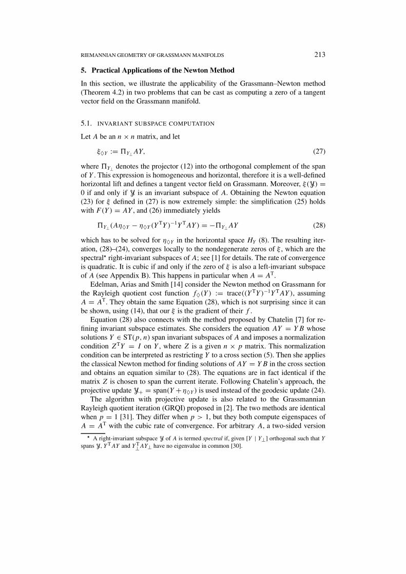
Table I.
Newton X+ = X − gradV/m
Iterate number ‖ ∑mi=1 δ
i dist(X,Y0) ‖∑mi=1 δ
i dist(X,Y0)
0 2.4561e + 01 2.9322e − 01 2.4561e + 01 2.9322e − 01
1 1.6710e + 00 3.1707e − 02 1.9783e + 01 2.1867e − 01
2 5.7656e − 04 2.0594e − 02 1.6803e + 01 1.6953e − 01
3 2.4207e − 14 2.0596e − 02 1.4544e + 01 1.4911e − 01
4 8.1182e − 16 2.0596e − 02 1.2718e + 01 1.2154e − 01
300 5.6525e − 13 2.0596e − 02
Yi = span([IpKi
]). The initial iterate is X := Y1 and we define Y0 = span(
[Ip0
]).
The experimental results are shown on Table I.
6. Conclusion
We have considered the Grassmann manifold Grass(p, n) of p-planes in Rn as the
base space of a GLp-principal fiber bundle with the noncompact Stiefel manifoldST(p, n) as the total space. Using the essentially unique On-invariant metric onGrass(p, n), we have derived a formula for the Levi-Civita connection in termsof horizontal lifts. Moreover, formulas have also been given for the Lie bracket,parallel translation, geodesics, and distance between p-planes. Finally, these resultshave been applied to a detailed derivation of the Newton method on the Grassmannmanifold. The Grassmann–Newton method has been illustrated by two examples.
Appendix A. Quadratic Convergence of Riemann–Newton
For completeness we include the proof of quadratic convergence of the Riemann–Newton iteration (Algorithm 4.1). Our proof significantly differs from the proofpreviously reported in the literature [33]. This proof also prepares the discussionon cubic convergence cases in Appendix B.
Let ξ be a smooth vector field on a Riemannian manifoldM and let ∇ denote theRiemannian connection. Let z ∈ M be a nondegenerate zero of the smooth vectorfield ξ (i.e. ξz = 0 and the linear operator TzM η �→ ∇ηξ ∈ TzM is invertible).Let Nz be a normal neighbourhood of z, sufficiently small so that any two pointsof Nz can be joined by a unique geodesic [6]. Let τxy denote the parallel transportalong the unique geodesic between x and y. Let the tangent vector ζ ∈ TxM bedefined by Expx ζ = z. Define the vector field ζ onNz adapted to the tangent vector
216 P.-A. ABSIL ET AL.
ζ ∈ TxM by ζy = τxyζ . Applying Taylor’s formula to the function λ �→ ξExpx λζ
yields [33]
0 = ξz = ξx + ∇ζ ξ + 1
2∇2ζ ξ + O(ζ 3), (29)
where ∇2ζ ξ := ∇ζ (∇ζ ξ ). Subtracting Newton equation (22) from Taylor’s formula
(29) yields
∇(η−ζ )ξ = ∇2ζ ξ + O(ζ 3). (30)
Since ξ is a smooth vector field and z is a nondegenerate zero of ξ , and reducingthe size of Nz if necessary, one has
‖∇αξ‖ � c1‖α‖,‖∇2
αξ‖ � c3‖α‖2
for all y ∈ Nz and α ∈ TyM. Using these results in (30) yields
c1‖η − ζ‖ � c2‖ζ‖2 + O(ζ 3). (31)
From now on the proof significantly differs from the one in [33]. We will shownext that, reducing again the size of Nz if necessary, there exists a constant c4 suchthat
dist(Expy α,Expy β) � c4‖α − β‖ (32)
for all y ∈ Nz and all α, β ∈ TyM small enough for Expy α and Expy β to be inNz. Then it follows immediately from (31) and (32) that
dist(x+, z) = dist(Expy η,Expy ζ )
� ‖η − ζ‖ � c2
c1‖ζ‖2 + O(ζ 3) = O(dist(x, z)2)
and this is the quadratic convergence.To show (32), we work in local coordinates covering Nz and use tensorial
notation (see, e.g., [6]), so, e.g., ui denotes the coordinates of u ∈ M. Considerthe geodesic equation ui + <ijk(u)u
i uj = 0 where < stands for the (smooth)Christoffel symbol, and denote the solution by φi[t, u(0), u(0)]. Then (Expy α)
i =φi[1, y, α], (Expy β)
i = φi[1, y, β], and the curve γ i: τ �→ φi[1, y, α+τ(β−α)]verifies γ i(0) = (Expy α)
i and γ i(1) = (Expy β)i . Then
dist(Expy α,Expy β)
�∫ 1
0
√gij [γ (τ)]γ i (τ )γ j (τ ) dτ (33)
=∫ 1
0
√gij [γ (τ)] ∂φ
i
∂uk[1, y, α + τ(β − α)]∂φ
i
∂u@[1, y, α + τ(β − α)](βk − αk)(β@ − α@) dτ
� c′√δk@(β
k − αk)(β@ − α@) (34)
� c4
√gk@[y](βk − αk)(β@ − α@) (35)
= c4‖β − α‖.
RIEMANNIAN GEOMETRY OF GRASSMANN MANIFOLDS 217
Equation (33) gives the length of the curve γ (0, 1), for which dist(Expy α,Expy β)is a lower bound. Equation (34) comes from the fact that the metric tensor gij andthe derivatives of φ are smooth functions defined on a compact set, thus bounded.Equation (35) comes because gij is nondegenerate and smooth on a compact set.
Appendix B. Cubic Convergence of Riemann–Newton
We use the notation of the previous section.If ∇2
αξ = 0 for all tangent vectors α ∈ TzM, then the rate of convergence of theRiemann–Newton method (Algorithm 4.1) is cubic. Indeed, by the smoothness ofξ , and defining ζx such that Expx ζ = z, one has ∇2
ζ ξ = O(ζ 3), and substitutingthis into (30) gives the result.
For the sake of illustration, we consider a particular case whereM is the Grass-mann manifold Grass(p, n) of p-planes in R
n, A is an n × n real matrix and thetangent vector field ξ is defined by the horizontal lift (27)
ξ♦Y = Y⊥AY,
where Y⊥ := (I − YY T). Let Z ∈ Grass(p, n) satisfy ξZ = 0, which happensif and only if Z is a right-invariant subspace of A. We show that ∇2
αξ = 0 forall α ∈ TZGrass(p, n) if and only if Z is a left-invariant subspace of A (whichhappens, e.g., when A = AT).
Let Z be an orthonormal basis for Z, i.e., ξ♦Z = 0 and ZTZ = I . Let α♦Z =U,V T be a thin singular value decomposition of α ∈ TZGrass(p, n). Then thecurve
Y (t) = ZV cos,t + U sin,t
is horizontal and projects through the ‘span’ operation to the Grassmann geodesicExpZ tα . Since by definition the tangent vector of a geodesic is parallel transportedalong the geodesic, the adaptation α of a verifies
α♦Y (t) = Y (t) = U, cos,t − ZV, cos,t.
Then one obtains successively
(∇αξ )♦Y (t) = Y(t)⊥Dξ♦(Y (t))[α♦Y (t)]= Y(t)⊥
d
dt Y(t)⊥AY(t)
= Y(t)⊥AY (t)− Y(t)⊥Y (t)Y (t)TAY(t)and
∇2αξ = (∇α∇αξ )♦Z
= Z⊥d
dt(∇αξ )♦Y (t)|t=0
218 P.-A. ABSIL ET AL.
= − Z⊥AY (0)− Z⊥Y (0)Y (0)TAY (0) −
− Z⊥ Y (0)(Y (0)TAY(0)+ Y (0)TAY (0))
= −2U,V TZTAU,,
where we have used Y⊥Y = 0, ZTU = 0, UTAZ = Z⊥AZ = 0. This lastexpression vanishes for all α ∈ TZGrass(p, n) if and only if UTATZ = 0 for all Usuch that UTZ = 0, i.e., Z is a left-invariant subspace of A.
Acknowledgements
The first author thanks P. Lecomte (Universite de Liege) and U. Helmke andS. Yoshizawa (Universitat Wurzburg) for useful discussions.
This paper presents research partially supported by the Belgian Programme onInter-university Poles of Attraction, initiated by the Belgian State, Prime Minister’sOffice for Science, Technology and Culture. Part of this work was performed whilethe first author was a guest at the Mathematisches Institut der Universität Würzburgunder a grant from the European Nonlinear Control Network. The hospitality ofthe members of the institute is gratefully acknowledged. The work was completedwhile the first and last authors were visiting the department of Mechanical andAerospace Engineering at Princeton University. The hospitality of the members ofthe department, especially Prof. N. Leonard, is gratefully acknowledged. The lastauthor thanks N. Leonard and E. Sontag for a partial financial support under USAir Force Grants F49620-01-1-0063 and F49620-01-1-0382.
References
1. Absil, P.-A.: Invariant subspace computation: A geometric approach, Ph.D. thesis, Faculté desSciences Appliquées, Université de Liège, Secrétariat de la FSA, Chemin des Chevreuils 1(Bât. B52), 4000 Liège, Belgium, 2003.
2. Absil, P.-A., Mahony, R., Sepulchre, R. and Van Dooren, P.: A Grassmann–Rayleigh quotientiteration for computing invariant subspaces, SIAM Rev. 44(1) (2002), 57–73.
3. Absil, P.-A., Sepulchre, R., Van Dooren, P. and Mahony, R.: Cubically convergent iterations forinvariant subspace computation, SIAM J. Matrix Anal. Appl., to appear.
4. Absil, P.-A. and Van Dooren, P.: Two-sided Grassmann–Rayleigh quotient iteration, SIAM J.Matrix Anal. Appl. (2002), submitted.
5. Björk, Å. and Golub, G. H.: Numerical methods for computing angles between linearsubspaces, Math. Comp. 27 (1973), 579–594.
6. Boothby, W. M.: An Introduction to Differentiable Manifolds and Riemannian Geometry,Academic Press, 1975.
7. Chatelin, F.: Simultaneous Newton’s iteration for the eigenproblem, Computing 5(Suppl.)(1984), 67–74.
8. Chavel, I.: Riemannian Geometry – A Modern Introduction, Cambridge Univ. Press, 1993.9. Common, P. and Golub, G. H.: Tracking a few extreme singular values and vectors in signal
processing, Proc. IEEE 78(8) (1990), 1327–1343.10. Demmel, J. W.: Three methods for refining estimates of invariant subspaces, Computing 38
(1987), 43–57.
RIEMANNIAN GEOMETRY OF GRASSMANN MANIFOLDS 219
11. Dennis, J. E. and Schnabel, R. B.: Numerical Methods for Unconstrained Optimizationand Nonlinear Equations, Prentice Hall Series in Computational Mathematics, Prentice-Hall,Englewood Cliffs, NJ, 1983.
12. do Carmo, M. P.: Riemannian Geometry, Birkhäuser, 1992.13. Doolin, B. F. and Martin, C. F.: Introduction to Differential Geometry for Engineers, Mono-
graphs and Textbooks in Pure and Applied Mathematics 136, Marcel Deckker, Inc., New York,1990.
14. Edelman, A., Arias, T. A. and Smith, S. T.: The geometry of algorithms with orthogonalityconstraints, SIAM J. Matrix Anal. Appl. 20(2) (1998), 303–353.
15. Ferrer, J., García, M. I. and Puerta, F.: Differentiable families of subspaces, Linear AlgebraAppl. 199 (1994), 229–252.
16. Gabay, D.: Minimizing a differentiable function over a differential manifold, J. Optim. TheoryAppl. 37(2) (1982), 177–219.
17. Golub, G. H. and Van Loan, C. F.: Matrix Computations, 3rd edn, The Johns Hopkins Univ.Press, 1996.
18. Helgason, S.: Differential Geometry, Lie Groups, and Symmetric Spaces, Pure Appl. Math. 80,Academic Press, Oxford, 1978.
19. Helmke, U. and Moore, J. B.: Optimization and Dynamical Systems, Springer, 1994.20. Karcher, H.: Riemannian center of mass and mollifier smoothing, Comm. Pure Appl. Math.
30(5) (1977), 509–541.21. Kendall, W. S.: Probability, convexity, and harmonic maps with small image. I. Uniqueness and
fine existence, Proc. London Math. Soc. 61(2) (1990), 371–406.22. Kobayashi, S. and Nomizu, K.: Foundations of Differential Geometry, Vol. 1, 2, Wiley, 1963.23. Leichtweiss, K.: Zur riemannschen Geometrie in grassmannschen Mannigfaltigkeiten, Math.
Z. 76 (1961), 334–366.24. Luenberger, D. G.: Optimization by Vector Space Methods, Wiley, Inc., 1969.25. Lundström, E. and Eldén, L.: Adaptive eigenvalue computations using Newton’s method on the
Grassmann manifold, SIAM J. Matrix Anal. Appl. 23(3) (2002), 819–839.26. Machado, A. and Salavessa, I.: Grassmannian manifolds as subsets of Euclidean spaces, Res.
Notes in Math. 131 (1985), 85–102.27. Mahony, R. E.: The constrained Newton method on a Lie group and the symmetric eigenvalue
problem, Linear Algebra Appl. 248 (1996), 67–89.28. Mahony, R. and Manton, J. H.: The geometry of the Newton method on non-compact Lie
groups, J. Global Optim. 23(3) (2002), 309–327.29. Nomizu, K.: Invariant affine connections on homogeneous spaces, Amer. J. Math. 76 (1954),
33–65.30. Ran, A. C. M. and Rodman, L.: A class of robustness problems in matrix analysis, In: D.
Alpay, I. Gohberg, and V. Vinnikov (eds), Interpolation Theory, Systems Theory and RelatedTopics, The Harry Dym Anniversary Volume, Operator Theory: Advances and Applications134, Birkhäuser, 2002, pp. 337–383.
31. Simoncini, V. and Elden, L.: Inexact Rayleigh quotient-type methods for eigenvalue computa-tions, BIT 42(1) (2002), 159–182.
32. Smith, S. T.: Geometric optimization methods for adaptive filtering, Ph.D. thesis, Division ofApplied Sciences, Harvard University, Cambridge, MA, 1993.
33. Smith, S. T.: Optimization techniques on Riemannian manifolds, In: A. Bloch (ed.), Hamil-tonian and Gradient Flows, Algorithms and Control, Fields Institute Communications, Vol. 3,Amer. Math. Soc., 1994, pp. 113–136.
34. Stewart, G. W.: Error and perturbation bounds for subspaces associated with certain eigenvalueproblems, SIAM Rev. 15(4) (1973), 727–764.
35. Udriste, C.: Convex Functions and Optimization Methods on Riemannian Manifolds, KluwerAcad. Publ., Dordrecht, 1994.
220 P.-A. ABSIL ET AL.
36. Wong, Y.-C.: Differential geometry of Grassmann manifolds, Proc. Nat. Acad. Sci. U.S.A. 57(1967), 589–594.
37. Woods, R. P.: Characterizing volume and surface deformations in an atlas framework: Theory,applications, and implementation, NeuroImage 18(3) (2003), 769–788.