Riemer PhD 2000

7/18/2019 Riemer PhD 2000

http://slidepdf.com/reader/full/riemer-phd-2000 1/285

MODELING CATHODIC PROTECTION FOR PIPELINE NETWORKS

By

DOUGLAS P. RIEMER

A DISSERTATION PRESENTED TO THE GRADUATE SCHOOL

OF THE UNIVERSITY OF FLORIDA IN PARTIAL FULFILLMENT

OF THE REQUIREMENTS FOR THE DEGREE OF

DOCTOR OF PHILOSOPHY

UNIVERSITY OF FLORIDA

2000

7/18/2019 Riemer PhD 2000


ACKNOWLEDGEMENTS

This work was jointly supported by the Pipeline Research Council Interna-

tional and the Gas Research Institute through Contract Number PR-101-9512.

ii

7/18/2019 Riemer PhD 2000


TABLE OF CONTENTS

Page

ACKNOWLEDGEMENTS . . . . . . . . . . . . . . . . . . . . . . . . . . . ii

LIST OF TABLES . . . . . . . . . . . . . . . . . . . . . . . . . . . . . . . . viii

LIST OF FIGURES . . . . . . . . . . . . . . . . . . . . . . . . . . . . . . . x

KEY TO SYMBOLS . . . . . . . . . . . . . . . . . . . . . . . . . . . . . . . xix

ABSTRACT . . . . . . . . . . . . . . . . . . . . . . . . . . . . . . . . . . . xxi

CHAPTERS

1 PIPELINES AND CATHODIC PROTECTION . . . . . . . . . . . . . . 1

1.1 Introduction . . . . . . . . . . . . . . . . . . . . . . . . . . . . . . . . 11.2 Electrode Kinetics (Butler-Volmer) . . . . . . . . . . . . . . . . . . . 7

1.3 Mixed Potential Kinetics . . . . . . . . . . . . . . . . . . . . . . . . . 101.4 Application to Corrosion in an Electrolyte . . . . . . . . . . . . . . 111.5 Passivation and Film Formation . . . . . . . . . . . . . . . . . . . . . 121.6 Coatings . . . . . . . . . . . . . . . . . . . . . . . . . . . . . . . . . . 131.7 Anode Polarization . . . . . . . . . . . . . . . . . . . . . . . . . . . . 16

1.7.1 Galvanic Anodes . . . . . . . . . . . . . . . . . . . . . . . . . 161.7.2 Impressed Current Anodes . . . . . . . . . . . . . . . . . . . 17

1.8 Conclusions . . . . . . . . . . . . . . . . . . . . . . . . . . . . . . . . 19

2 MATHEMATICAL DEVELOPMENT . . . . . . . . . . . . . . . . . . . 21

2.1 Soil Domain . . . . . . . . . . . . . . . . . . . . . . . . . . . . . . . . 21

2.2 Justification of Dilute Approximation . . . . . . . . . . . . . . . . . 242.3 Internal Domain . . . . . . . . . . . . . . . . . . . . . . . . . . . . . . 252.4 Quasipotential Transformation . . . . . . . . . . . . . . . . . . . . . 262.5 Conclusions . . . . . . . . . . . . . . . . . . . . . . . . . . . . . . . . 28

iii

7/18/2019 Riemer PhD 2000


3 SOLUTION OF GOVERNING PDE . . . . . . . . . . . . . . . . . . . . 29

3.1 Boundary Element Method Development . . . . . . . . . . . . . . . 303.2 Symmetric Galerkin Boundary Element Method . . . . . . . . . . . 32

3.3 Boundary Conditions . . . . . . . . . . . . . . . . . . . . . . . . . . . 343.3.1 Bare Steel . . . . . . . . . . . . . . . . . . . . . . . . . . . . . 343.3.2 Coated Steel . . . . . . . . . . . . . . . . . . . . . . . . . . . . 353.3.3 Anodes . . . . . . . . . . . . . . . . . . . . . . . . . . . . . . . 35

3.4 Infinite Domains . . . . . . . . . . . . . . . . . . . . . . . . . . . . . 363.5 Half Spaces . . . . . . . . . . . . . . . . . . . . . . . . . . . . . . . . . 373.6 Layers . . . . . . . . . . . . . . . . . . . . . . . . . . . . . . . . . . . 383.7 Development of Finite Element Method for Internal Domain . . . . 41

3.7.1 Pipe Shell Elements . . . . . . . . . . . . . . . . . . . . . . . . 433.7.2 Applying Elements to the FEM . . . . . . . . . . . . . . . . . 44

3.8 Bonds and Resistors . . . . . . . . . . . . . . . . . . . . . . . . . . . . 46

3.9 Coupling BEM to FEM . . . . . . . . . . . . . . . . . . . . . . . . . . 473.10 Current Flow in the Pipe . . . . . . . . . . . . . . . . . . . . . . . . . 483.11 Conclusions . . . . . . . . . . . . . . . . . . . . . . . . . . . . . . . . 54

4 APPLYING KINETICS TO THE BEM AND FEM . . . . . . . . . . . . 55

4.1 Pipe Discretization . . . . . . . . . . . . . . . . . . . . . . . . . . . . 554.1.1 Discretization of the Boundary Element Method . . . . . . . 564.1.2 Discretization of the Finite Element Domain . . . . . . . . . 58

4.2 Self-Equilibration . . . . . . . . . . . . . . . . . . . . . . . . . . . . . 594.3 Multiple CP Systems . . . . . . . . . . . . . . . . . . . . . . . . . . . 604.4 Coating Holidays . . . . . . . . . . . . . . . . . . . . . . . . . . . . . 614.5 Nonlinear Boundary Conditions without Attenuation in the Pipe

Steel . . . . . . . . . . . . . . . . . . . . . . . . . . . . . . . . . . . . 624.6 Nonlinear Boundary Conditions with Attenuation in the Pipe Steel 664.7 Solution by Successive Substitutions . . . . . . . . . . . . . . . . . . 674.8 Solution of Combined System by Newton-Raphson Technique . . . 684.9 Variable Transformation to Stabilize Convergence . . . . . . . . . . 714.10 Conclusions . . . . . . . . . . . . . . . . . . . . . . . . . . . . . . . . 74

5 MESH GENERATION . . . . . . . . . . . . . . . . . . . . . . . . . . . 75

5.1 Basic Mesh . . . . . . . . . . . . . . . . . . . . . . . . . . . . . . . . . 76

5.1.1 Discretization and Shape Functions . . . . . . . . . . . . . . 765.1.2 Continuity of the Shape Functions . . . . . . . . . . . . . . . 785.1.3 Quadratic Iso-Parametric Rectangles . . . . . . . . . . . . . . 815.1.4 Quadratic Triangles . . . . . . . . . . . . . . . . . . . . . . . . 83

5.2 Long Pipes . . . . . . . . . . . . . . . . . . . . . . . . . . . . . . . . . 845.3 Holidays . . . . . . . . . . . . . . . . . . . . . . . . . . . . . . . . . . 85

5.3.1 Round Holidays . . . . . . . . . . . . . . . . . . . . . . . . . 86

iv

7/18/2019 Riemer PhD 2000


5.3.2 Rectangular Holidays . . . . . . . . . . . . . . . . . . . . . . 915.4 Pipe Crossings and Shadowing . . . . . . . . . . . . . . . . . . . . . 925.5 Soil Type Divisions . . . . . . . . . . . . . . . . . . . . . . . . . . . . 925.6 Conclusions . . . . . . . . . . . . . . . . . . . . . . . . . . . . . . . . 95

6 SOLUTION ACCURACY . . . . . . . . . . . . . . . . . . . . . . . . . 96

6.1 Sources of Error . . . . . . . . . . . . . . . . . . . . . . . . . . . . . . 966.2 Integration Accuracy . . . . . . . . . . . . . . . . . . . . . . . . . . . 976.3 Integration Techniques . . . . . . . . . . . . . . . . . . . . . . . . . . 98

6.3.1 Adaptive Integration . . . . . . . . . . . . . . . . . . . . . . . 996.3.2 Singular Integrals . . . . . . . . . . . . . . . . . . . . . . . . . 101

6.4 Matrix Inversions . . . . . . . . . . . . . . . . . . . . . . . . . . . . . 101

7 MODEL VERIFICATION . . . . . . . . . . . . . . . . . . . . . . . . . 103

7.1 Primary Current Distribution to a Disk . . . . . . . . . . . . . . . . . 1047.1.1 Disk in a Half Space . . . . . . . . . . . . . . . . . . . . . . . 1047.1.2 Disk-Shaped Coating Holiday . . . . . . . . . . . . . . . . . 106

7.2 Comparison to the Solution of Kasper . . . . . . . . . . . . . . . . . 1087.3 Dwight’s Equation . . . . . . . . . . . . . . . . . . . . . . . . . . . . 108

8 SOLUTION VISUALIZATION AND INTERFACE DESIGN . . . . . . . 113

8.1 Interface Design . . . . . . . . . . . . . . . . . . . . . . . . . . . . . . 1138.2 Data Visualization . . . . . . . . . . . . . . . . . . . . . . . . . . . . . 1158.3 2D Solution Visualization . . . . . . . . . . . . . . . . . . . . . . . . 116

8.4 3D Visualization . . . . . . . . . . . . . . . . . . . . . . . . . . . . . . 1198.4.1 Using OpenGL . . . . . . . . . . . . . . . . . . . . . . . . . . 1198.4.2 Coding OpenGL for BEM and FEM Meshes . . . . . . . . . . 123

8.5 Visual Feedback . . . . . . . . . . . . . . . . . . . . . . . . . . . . . . 124

9 COMPUTATIONAL PERFORMANCE . . . . . . . . . . . . . . . . . . 125

9.1 Parrallel Computing Methods . . . . . . . . . . . . . . . . . . . . . . 1259.2 Processor Arrays . . . . . . . . . . . . . . . . . . . . . . . . . . . . . 1269.3 Distributed Computation Methods . . . . . . . . . . . . . . . . . . . 1279.4 Communication Between Computers . . . . . . . . . . . . . . . . . . 1289.5 Improving Performance by Separating Calculation Code . . . . . . 1299.6 Benchmarks and Scaling . . . . . . . . . . . . . . . . . . . . . . . . . 1309.7 Hard Drive Performance . . . . . . . . . . . . . . . . . . . . . . . . . 1349.8 High Performance Libraries . . . . . . . . . . . . . . . . . . . . . . . 136

v

7/18/2019 Riemer PhD 2000


10 HOLIDAY EFFECTS . . . . . . . . . . . . . . . . . . . . . . . . . . . . 137

10.1 Single Pipes . . . . . . . . . . . . . . . . . . . . . . . . . . . . . . . . 13810.2 Two Pipes with a Coating Flaw . . . . . . . . . . . . . . . . . . . . . 140

10.3 Pipes Exhibiting Stray Current . . . . . . . . . . . . . . . . . . . . . 14210.4 Soil Surface On-Potentials . . . . . . . . . . . . . . . . . . . . . . . . 14610.5 Adjacent Holidays . . . . . . . . . . . . . . . . . . . . . . . . . . . . 147

11 COUPONS . . . . . . . . . . . . . . . . . . . . . . . . . . . . . . . . . 150

11.1 Introduction . . . . . . . . . . . . . . . . . . . . . . . . . . . . . . . . 15011.2 Boundary Condition Parameters . . . . . . . . . . . . . . . . . . . . 15311.3 Approach . . . . . . . . . . . . . . . . . . . . . . . . . . . . . . . . . . 15411.4 Results and Discussion . . . . . . . . . . . . . . . . . . . . . . . . . . 15611.5 Coupon Performance Diagram . . . . . . . . . . . . . . . . . . . . . 16111.6 Conclusion . . . . . . . . . . . . . . . . . . . . . . . . . . . . . . . . . 163

12 TANK BOTTOMS . . . . . . . . . . . . . . . . . . . . . . . . . . . . . 165

12.1 Tank Bottom Mesh . . . . . . . . . . . . . . . . . . . . . . . . . . . . 16612.2 Model for oxygen consumption . . . . . . . . . . . . . . . . . . . . . 16812.3 Implementation . . . . . . . . . . . . . . . . . . . . . . . . . . . . . . 17212.4 Results . . . . . . . . . . . . . . . . . . . . . . . . . . . . . . . . . . . 173

12.4.1 Remote Ground-bed . . . . . . . . . . . . . . . . . . . . . . . 17312.4.2 Distributed Anodes . . . . . . . . . . . . . . . . . . . . . . . . 17812.4.3 Ribbon Anodes . . . . . . . . . . . . . . . . . . . . . . . . . . 184

12.5 Conclusions . . . . . . . . . . . . . . . . . . . . . . . . . . . . . . . . 191

13 MULTIPLE SOIL DOMAINS . . . . . . . . . . . . . . . . . . . . . . . 193

13.1 Continuity Equations . . . . . . . . . . . . . . . . . . . . . . . . . . . 19313.2 Implementation . . . . . . . . . . . . . . . . . . . . . . . . . . . . . . 19513.3 Steel Resistance in Multiple Soil Domains . . . . . . . . . . . . . . . 197

14 CONCLUSIONS AND FUTURE WORK . . . . . . . . . . . . . . . . . 200

14.1 Conclusions . . . . . . . . . . . . . . . . . . . . . . . . . . . . . . . . 20014.2 Future Work . . . . . . . . . . . . . . . . . . . . . . . . . . . . . . . . 201

APPENDICES

A PARTIAL DERIVATIVES OF THE BOUNDARY CONDITIONS . . . . 203

vi

7/18/2019 Riemer PhD 2000


B OpenGL CODE . . . . . . . . . . . . . . . . . . . . . . . . . . . . . . 205

B.1 The OpenGL Device . . . . . . . . . . . . . . . . . . . . . . . . . . . 205B.2 The Drawing Cycle . . . . . . . . . . . . . . . . . . . . . . . . . . . . 208

B.3 Platform Independent Code . . . . . . . . . . . . . . . . . . . . . . . 209B.4 Using the Mouse for Interaction . . . . . . . . . . . . . . . . . . . . . 212B.4.1 Orienting an Object . . . . . . . . . . . . . . . . . . . . . . . . 212B.4.2 Selecting Objects . . . . . . . . . . . . . . . . . . . . . . . . . 218

C CODE STRUCTURE . . . . . . . . . . . . . . . . . . . . . . . . . . . . 222

C.1 Interface . . . . . . . . . . . . . . . . . . . . . . . . . . . . . . . . . . 222C.1.1 Data Management . . . . . . . . . . . . . . . . . . . . . . . . 224C.1.2 Data Interaction . . . . . . . . . . . . . . . . . . . . . . . . . . 227

C.2 Calculation Engine . . . . . . . . . . . . . . . . . . . . . . . . . . . . 232C.2.1 Assembly of Boundary Element Matrices . . . . . . . . . . . 232C.2.2 Assembly of Finite Element Matrices . . . . . . . . . . . . . . 233C.2.3 Solution of Nonlinear System . . . . . . . . . . . . . . . . . . 234C.2.4 Soil Surface On-Potentials . . . . . . . . . . . . . . . . . . . . 239

C.3 Remote Integration . . . . . . . . . . . . . . . . . . . . . . . . . . . . 239C.3.1 Interface Definition . . . . . . . . . . . . . . . . . . . . . . . . 240C.3.2 Data Marshaling . . . . . . . . . . . . . . . . . . . . . . . . . 242C.3.3 Server Side . . . . . . . . . . . . . . . . . . . . . . . . . . . . . 243C.3.4 Client Side . . . . . . . . . . . . . . . . . . . . . . . . . . . . . 245

REFERENCES . . . . . . . . . . . . . . . . . . . . . . . . . . . . . . . . . . 252

BIOGRAPHICAL SKETCH . . . . . . . . . . . . . . . . . . . . . . . . . . . 263

vii

7/18/2019 Riemer PhD 2000


LIST OF TABLES

Table page

1.1 Parameters for common galvanic anodes. . . . . . . . . . . . . . . . 17

1.2 Parameters for the oxygen and chlorine evolution reactions. . . . . 19

5.1 Error of Constant, Linear, and Quadratic elements in representinga circle whose circumference is π and has unit diameter. . . . . . . . 78

9.1 Comparison of location of integration source code. . . . . . . . . . . 129

9.2 Normalized benchmark result data for many types of computers. . 131

9.3 An example run of the scaling of a heterogeneous distributed com-puter. . . . . . . . . . . . . . . . . . . . . . . . . . . . . . . . . . . . . 133

9.4 An second example run of the scaling of a heterogeneous distributedcomputer. This run shows better scaling because the load fromother users was less. . . . . . . . . . . . . . . . . . . . . . . . . . . . 134

9.5 Conditions used for all hard drive performance tests . . . . . . . . . 135

9.6 Implementing Vector operations in the Residual Vector Calculation 135

9.7 Implementing Vector operations in building the A matrix . . . . . . 135

11.1 Polarization parameters used in the model. . . . . . . . . . . . . . . 153

11.2 Coating parameters used in model. Note: These parameters were

determined after water uptake of the coating. . . . . . . . . . . . . . 154

11.3 Results of two coupon model. The small coupon used a polariza-tion curve with i lim,O2

= 1.0 µA/cm2 (curve 1). The large couponused ilim,O2

that was an order of magnitude smaller (curve 2). . . . . 160

viii

7/18/2019 Riemer PhD 2000


11.4 Results of two coupon model. The large coupon used a polariza-tion curve with i lim,O2

= 1.0 µA/cm2 (curve 1). The small couponused a ilim,O2

that was an order of magnitude lower(curve 2). . . . . 160

ix

7/18/2019 Riemer PhD 2000


LIST OF FIGURES

Figure page

1-1 Post explosion flare-off of leaking gas from a burst pipeline. The burst was later attributed to corrosion weakened walls of the pipe. 2

1-2 Failed section of the butane pipe. a) an overview showing the sizeof the ruptured seam; b) a closeup of the failed section of pipe. The

burst seam in the pipe followed a line of severe corrosion. . . . . . 3

1-3 Pipe and anode system used for cathodic protection of buried pipelines.The anode is the smaller vertical cylinder on the right. The redcylinder in-line with the connecting wire is a resistor that is usu-ally inserted in the circuit to control the amount of current drivento the pipe in order to limit hydrogen evolution. . . . . . . . . . . . 5

1-4 Pouraix diagram for iron. . . . . . . . . . . . . . . . . . . . . . . . . 13

1-5 Diagram of coating model. . . . . . . . . . . . . . . . . . . . . . . . . 14

1-6 Typical polarization curves associated with bare and coated steel. . 16

3-1 Symmetric integration. Lines between the two circles represent theGreen’s function relation between the two integration points onthe surfaces dΓ i and dΓ j . . . . . . . . . . . . . . . . . . . . . . . . . . 34

3-2 Reflections of Green’s function to account for boundaries with zeronormal current. . . . . . . . . . . . . . . . . . . . . . . . . . . . . . . 39

3-3 Rectangular enclosure created with a primary Green’s function and6 reflections. . . . . . . . . . . . . . . . . . . . . . . . . . . . . . . . . 40

3-4 Total cathodic current driven to a pipe with an underlying non-conducting region. . . . . . . . . . . . . . . . . . . . . . . . . . . . . 40

3-5 Fit of the data from Figure 3-4 to i = −0.064√ r + 0.2118. . . . . . . . . . 42

x

7/18/2019 Riemer PhD 2000


3-6 Diagram of the shell element used to calculate the potential dropwithin the pipe steel. The element is assumed to have no variationin the ζ direction. The curvilinear coordinate system is displayedon top of the element. . . . . . . . . . . . . . . . . . . . . . . . . . . . 43

3-7 Black lines connecting pipes and anode are bonds. The red cylin-ders represent resistors. They are modeled as 1-D finite elementsthat connect to the bond connection points. . . . . . . . . . . . . . . 47

3-8 Normalized current vectors drawn on top of the pipe. Three com-ponents of the vectors are calculated in cartesian coordinates eventhough the flow of current is only in two directions. The fact thatthe vectors are always tangent to the pipe indicates that the coor-dinate transformation was done correctly. . . . . . . . . . . . . . . . 53

4-1 Newton-Raphson line search flow diagram. . . . . . . . . . . . . . . 65

5-1 Type of mesh needed for model. Three pipes are shown passingthrough a point where the soil conductivity changes. . . . . . . . . 75

5-2 Circle discretized with 8 linear triangular elements. The area is

2√

2r2 for the 8 triangles which is a 10.% error. . . . . . . . . . . . . 77

5-3 Four quadratic elements with eight degrees of freedom represent-

ing a circle. . . . . . . . . . . . . . . . . . . . . . . . . . . . . . . . . . 79

5-4 Continuity of the basis functions. Two elements are shown. Basisfunctions that share a node with a value of one must be continuous. 80

5-5 Use of triangles to increase the degrees of freedom in the centerregion while maintaining C0 continuity. . . . . . . . . . . . . . . . . 81

5-6 Quadratic iso-parametric rectangular parent element. Numberingof nodes and shape functions given in figure. . . . . . . . . . . . . . 82

5-7 Quadratic iso-parametric triangular parent element. Numberingof nodes and shape functions given in figure. . . . . . . . . . . . . . 83

5-8 Decrease of element aspect ratio at a boundary condition change. . 85

xi

7/18/2019 Riemer PhD 2000


5-9 Current density distribution on a circular holiday. Parameter J is afunction of the average current density iavg, the inverse Tafel slopeαc FRT

, the holiday radius ro, and the soil resistivity κ. . . . . . . . . . . 87

5-10 A mesh that includes two round holidays. This is the output froma standard mesh generator. Further processing is needed to mapthe mesh to a pipe and adjust the holidays so they are round. . . . . 88

5-11 The same mesh as shown in Figure 5-10. Here the elements for theholiday have been removed. The elements have been divided intofour triangles to illustrate the locations of the center nodes on eachside of the triangles. . . . . . . . . . . . . . . . . . . . . . . . . . . . 89

5-12 The same mesh as shown in Figures 5-10 and 5-11. The nodes on aholiday boundary that did not lie on the circle defining the holiday

have been moved for the large holiday. The task has not yet beendone for the small holiday. . . . . . . . . . . . . . . . . . . . . . . . 90

5-13 A gouge at the bottom of a pipe that was meshed using rectangularelements. . . . . . . . . . . . . . . . . . . . . . . . . . . . . . . . . . 90

5-14 Closeup of one edge of a rectangular holiday where two triangleshave been used to increase the element density of the holiday. . . . 91

5-15 Mesh at a crossing of two pipes. Both pipes have the highest den-sity of elements at the crossing point. . . . . . . . . . . . . . . . . . . 93

5-16 Output of the Delauny mesh generator when creating a division between two soil domains. The holes for the pipes need post-processing before the mesh can be used. . . . . . . . . . . . . . . . . 94

5-17 Completed mesh with pipes passing through soil type division. . . 94

6-1 Sub-element with a high aspect ratio subdivided by the adaptiveintegration routine to reduce the aspect ratio of the subsections. . . 100

6-2 Sub-element with a desired aspect ratio subdivided by the adap-tive integration routine. . . . . . . . . . . . . . . . . . . . . . . . . . 100

xii

7/18/2019 Riemer PhD 2000


7-1 Primary current distribution on a disk electrode in a half-plane.Model solution at center of disk is within 2.0% of the analytic so-lution of i/iavg = 0.5. This view is looking along the z axis towardthe disk. . . . . . . . . . . . . . . . . . . . . . . . . . . . . . . . . . . 105

7-2 Comparison of primary current distribution on a disk electrode ina half-plane. Red line without circles is the analytic solution, blueline is the numerical solution from the disk shown in Figure 7-1. . 105

7-3 Disk holiday on a pipe. Shading corresponds to the off-potential.Note the draw-down of potential in the coated region around theholiday. . . . . . . . . . . . . . . . . . . . . . . . . . . . . . . . . . . 106

7-4 Comparison of current density at the center of a disk electrode ina half-plane (solid line) to that of a disk shaped holiday on a pipe

(circles). . . . . . . . . . . . . . . . . . . . . . . . . . . . . . . . . . . 107

7-5 Solution to the current distribution on a cylinder given by Kasper.Plot represents the ratio of the maximum to minimum current den-sity. At infinite separation, the ratio becomes 1. . . . . . . . . . . . . 109

7-6 Distribution of current around half the circumference when thecylinders are placed at 3.0 diameters separation. The ratio of themax current to the min is 0.72. Kasper’s solution is 0.78 . . . . . . . 110

7-7 Error in Dwight’s equation as a function of the separation of two

cylinders. Solution given by the 3 dimensional model approachesDwight’s solution at large separation. The difference between Dwight’ssolution and the model is due to end effects. . . . . . . . . . . . . . 111

8-1 A screen shot and movie (click on image above) that shows some of the interactive graphics techniques needed for three dimensionalgeometry. . . . . . . . . . . . . . . . . . . . . . . . . . . . . . . . . . . 113

8-2 A screen shot of the basic window used for the interface to themodel. The window contains elements familiar to anyone who

uses MicrosoftWindows. . . . . . . . . . . . . . . . . . . . . . . . 114

8-3 A screen shot of the basic window with an empty model. The win-dow has two parts: the first is for control and feedback, the otheris for data display in 3 dimensions. . . . . . . . . . . . . . . . . . . . 115

xiii

7/18/2019 Riemer PhD 2000


8-4 Red line represents the points of the pipe surface that are extractedto create a X-Y plot. X values are the how far from the startingend of the pipe the value of the potential, current, off-potential, orcorrosion current is taken. . . . . . . . . . . . . . . . . . . . . . . . . 117

8-5 The red line represents the points of the pipe surface that are ex-tracted to create a X-Y plot. X values are the how far from the start-ing end of the pipe the value of the potential, current, off-potential,or corrosion current is taken. . . . . . . . . . . . . . . . . . . . . . . 118

8-6 Shaded mesh of boundary element calculation grid. OpenGL al-lows instant visual inspection of the mesh for correctness. . . . . . . 121

8-7 Same view as figure 8-6 on page 121, with four times the number of elements. This has been done to better approximate the quadratic

nature of the real elements using linear interpolation for the graph-ics elements. . . . . . . . . . . . . . . . . . . . . . . . . . . . . . . . . 122

9-1 Plot of performance vs expected performance for a distributed com-puter. . . . . . . . . . . . . . . . . . . . . . . . . . . . . . . . . . . . . 129

10-1 Pipe that exhibits many coating holidays. Pipe was coated in thelate 60’s and dug up in 1996. . . . . . . . . . . . . . . . . . . . . . . . 137

10-2 Off-potential distribution for a large holiday in a good quality coat-ing. The edge of the coating next to the holiday does not meet the-850 mV criterion while the holiday does. Even so, the corrosionrate at the holiday is much higher than at any of the coated sections. 139

10-3 Current density and potential distribution around the circumfer-ence of a pipe through a holiday. Zero degrees is the top of thepipe. The blue line is the current density. . . . . . . . . . . . . . . . 140

10-4 Current density and potential distribution around the circumfer-ence of a pipe through an under-protected holiday. Zero degrees

is the top of the pipe. The blue line is the current density. . . . . . . 141

10-5 Current density and potential distribution around the circumfer-ence of a pipe at the spot closest to the under-protected holiday onthe neighboring pipe. Zero degrees is the top of the pipe. The blueline is the current density. . . . . . . . . . . . . . . . . . . . . . . . . 142

xiv

7/18/2019 Riemer PhD 2000


10-6 Distant view of a under-protected holiday. Lower right portion of pipe with holiday is also exhibiting stray current. . . . . . . . . . . 143

10-7 Closeup of an under-protected holiday. . . . . . . . . . . . . . . . . 144

10-8 Current Density around pipe in area exhibiting stray current inFigure 10-7. Positive current densities are anodic. . . . . . . . . . . 145

10-9 Potential distribution around pipe at center of section exhibitingstray current and at end of section where all parts of the circumfer-ence of the pipe are cathodic. . . . . . . . . . . . . . . . . . . . . . . 145

10-10Distant view of soil surface on-potentials over an under-protectedholiday. . . . . . . . . . . . . . . . . . . . . . . . . . . . . . . . . . . . 146

10-11Distant view of soil surface on-potentials with a portion of the soilsurface removed to see the pipe. The soil surface on-potential onlyindicates the presence of the anodes. The holiday is not seen. . . . . 147

10-12Setup for calculation of a pinhole holiday next to a large holiday. . 148

10-13Off-potential distribution of a pinhole holiday next to a large hol-iday. The large holiday is under-protected by standard criteriawhile the pinhole is well protected. . . . . . . . . . . . . . . . . . . . 149

11-1 Schematic representations of the two cylindrical coupons used inthe simulations: a) large coupon with a surface area of ∼ 50 cm2;and b) smaller coupon with a surface area of 9.5 cm2 . . . . . . . . . 155

11-2 Large coupon - Difference between the most positive potential of the holiday and the coupon at three different rectifier outputs thatresult in the coupon potential being measured at -750, -850 and-950 mV (CSE). The negative sign on y-axis label indicates the hol-iday is at a potential cathodic to the coupon. The lack of a signindicates the opposite. Panels a) through d) correspond to differ-ent values of ξ = Aholiday/ Acoupon. . . . . . . . . . . . . . . . . . . . . 157

xv

7/18/2019 Riemer PhD 2000


11-3 Small coupon - Difference between the most positive potential of the holiday and the coupon at three different rectifier outputs thatresult in the coupon potential being measured at -750, -850 and-950 mV (CSE). The negative sign on y-axis label indicates the hol-

iday is at a potential cathodic to the coupon. The lack of a signindicates the opposite. Panels a) through d) correspond to differ-ent values of ξ = Aholiday/ Acoupon. . . . . . . . . . . . . . . . . . . . . 158

11-4 Coupon performance diagram for coupons placed in the same soilenvironment as the pipeline coating defects that expose bare steel.The soil resistivity was 10,000 Ω cm. Black symbols correspondto calculations where a protected coupon corresponded to a pro-tected coating holiday. Open symbols correspond to calculationswhere the coupon could indicate adequate protection for pipeswith coating holidays that are seriously underprotected. The gray

symbols correspond to cases where the coupon reading is not con-servative, but the error was less than 15 mV. . . . . . . . . . . . . . . 162

12-1 High resolution mesh used for the boundary element mesh. . . . . 167

12-2 Oxygen concentration profile within the soil at several values of

the scaling parameter R

k /D. . . . . . . . . . . . . . . . . . . . . . 171

12-3 Potential distribution when the oxygen concentration is uniformat its largest value. This condition occurs when the tank has been

recently filled after being empty. The grid spacing is 10 ft square. . 175

12-4 Radial potential and current density distribution when the oxygenconcentration is uniform and at c∞. Potential is given by the redline. The black line indicates where a uniform current density dis-tribution would be. . . . . . . . . . . . . . . . . . . . . . . . . . . . . 176

12-5 Potential distribution when the oxygen concentration follows the

profile given in Figure 12-2 corresponding to R

k /D = 2.0. Thegrid spacing is 10 ft square. . . . . . . . . . . . . . . . . . . . . . . . 177

12-6 Radial potential and current density distribution when the oxygenconcentration follows the profile given in Figure 12-2 correspond-

ing to R

k /D = 2.0. Potential is given by the red line. The blackline indicates where a uniform current density distribution would

be. . . . . . . . . . . . . . . . . . . . . . . . . . . . . . . . . . . . . . . 178

xvi

7/18/2019 Riemer PhD 2000


12-7 Potential distribution with distributed anodes and uniform oxygenconcentration profile. . . . . . . . . . . . . . . . . . . . . . . . . . . . 180

12-8 Current density distribution on tank bottom with distributed an-

odes and uniform oxygen concentration. . . . . . . . . . . . . . . . . 180

12-9 Potential distribution with distributed anodes and nonuniform oxy-gen concentration profile. . . . . . . . . . . . . . . . . . . . . . . . . 182

12-10Potential and current density distribution on a tank bottom withdistributed anodes and nonuniform oxygen concentration. . . . . . 182

12-11Potential distribution with distributed anodes, underlying insulat-ing layer at 2 ft and uniform oxygen concentration profile. . . . . . 183

12-12Potential distribution with distributed anodes, underlying insulat-ing layer at 2 ft and nonuniform oxygen concentration profile. . . . 184

12-13Tank bottoms with 5 and 11 parallel impressed current anodes. . . . 185

12-14Potential distribution for tank bottoms with 5 and 11 parallel im-pressed current anodes with secondary containment. . . . . . . . . 186

12-15Axial current density distributions on anodes for both the 5 and 11anode cases. . . . . . . . . . . . . . . . . . . . . . . . . . . . . . . . . 188

12-16Potential and corrosion current distribution for tank bottoms with5 parallel impressed current anodes with no secondary containment.188

12-17Potential distribution for tank bottoms with 5 and 11 parallel im-pressed current anodes and secondary containment with nonuni-form oxygen distribution. . . . . . . . . . . . . . . . . . . . . . . . . 189

12-18Potential distribution for tank bottoms with 5 and 11 parallel im-pressed current anodes with nonuniform oxygen distribution. . . . 190

13-1 Plane meshed for a soil type change. Three pipes are shown pass-ing through a point where the soil conductivity changes. . . . . . . 194

13-2 Three domain model setup utilizing two soil division meshes. Thesoil surface grid is drawn using 1 mile squares. There are two pipesof 24 in diameter in a 50 ft right-of-way. . . . . . . . . . . . . . . . . 198

xvii

7/18/2019 Riemer PhD 2000


B-1 A movie demonstrating how the user can use the middle mouse button the change the OpenGL view of two pipelines. This is oneof the modes of movement. The movie is accessed by clicking onthe above image. . . . . . . . . . . . . . . . . . . . . . . . . . . . . . 214

C-1 Interface with two section:One for feedback and control, one for3D data display. . . . . . . . . . . . . . . . . . . . . . . . . . . . . . . 223

C-2 Console Window . . . . . . . . . . . . . . . . . . . . . . . . . . . . . 228

xviii

7/18/2019 Riemer PhD 2000


KEY TO SYMBOLS

Φ = Potential and potential distribution

V = Voltage distribution in the pipe steel and anode material

i = Current density

Ei = Equilibrium potential for species i

β i = Tafel slope

F = Faraday’s constant

R = Gas constant

T = Temperature

k = Kinetic parameter

κ = Conductivity

ci = Concentration of species i

t = Time

J i = Flux vector of species due to fields

Ni = Net flux vector of species i

Ri = Rate of generation of species i

Di = Diffusion coefficient for species i

zi = Charge on species i

ui = Mobility of species i

I = Ionic strength

xix

7/18/2019 Riemer PhD 2000


qi = Kirchhoff transformation variable for species i

Q = Quasi-potential

Ω = Domain for which a differential equation applies

Γ = Boundary of a domain

n = Outward normal vector of boundary

w = Arbitrary weighting function

G = Green’s function

ξ = Source point in Green’s function

x = Field point in Green’s function

δ = Dirac delta function

r = Euclidian distance between two points

G = Matrix of coefficients from the right hand integral of 3-9

H = Matrix of coefficients from the left hand integral of 3-9

A = Matrix of columns from the H and G matrices

Ψ = defined as V −Φ

n = Outward normal vector of boundary

K = Matrix resulting from Finite Element Method

n = total number of nodes in a problem

ne =

total number of elements in a problem

nen = number of nodes in an element

nce = number of elements having a given node in common

xx

7/18/2019 Riemer PhD 2000


Abstract of Thesis Presented to the Graduate School

of the University of Florida in Partial Fulfillment of theRequirements for the Degree of Doctor of Philosophy

MODELING CATHODIC PROTECTION FOR PIPELINE NETWORKS

By

Douglas P. Riemer

December 2000

Chair: Dr. Mark E. Orazem

Major Department: Chemical Engineering

An extensive network of buried steel pipelines is used throughout the world

to transport natural gas and liquid petroleum products. In the United States

alone, there are over 1.3 million miles of pipe used to transport natural gas. Fail-

ure to prevent external corrosion of pipelines can have disastrous consequences.

A butane line explosion, which cost the lives of two persons, was caused by exter-

nal corrosion attributed to inadequate cathodic protection. Proper cathodic pro-

tection is particularly important today because the pipelines constructed during

the construction boom of the 1960s and 1970s are aging, and the encroachment of

suburban housing construction increases the potential for property damage and

loss of life.

Standard cathodic protection design equations, based on the assumptions

that pipes are isolated and have a uniform bare metal surface, are not valid for

modern complex pipeline networks. The object of this work was to develop a

xxi

7/18/2019 Riemer PhD 2000


mathematical model that can describe correctly the complex interactions seen in

cathodic protection of complex pipeline networks. The governing differential

equation is solved in 3-dimensions for the conductance of current through thesoil, steel, and connections between pipes and anodes. The model accounts for

the kinetics of the corrosion, mass-transfer-limited oxygen reduction, and hydro-

gen evolution reactions. It also accounts for the nonuniform current and potential

distributions due to pipe-pipe interactions, coating flaws, and anode locations.

Current and potential distributions are calculated around the circumference and

along the length of the pipes.This dissertation describes the solution techniques needed to solve the sys-

tem of equations that couple nonlinear reaction kinetics, passage of current through

soil, and passage of current through pipeline steel. Sample calculations will be

presented to show the complicated nature of the interactions between adjacent

pipelines.

xxii

7/18/2019 Riemer PhD 2000


CHAPTER 1PIPELINES AND CATHODIC PROTECTION

1.1 Introduction

Since the beginning of the 20th century, petroleum products and natural gas

have been transported over long distances by buried steel pipelines. There are

over 1.28 million miles of buried steel main-line pipe for the transport of natural

gas alone. 1 There are, in addition, 170,000 miles of pipeline for transport of crude

oil and refined products.2

These pipes are generally in soil environments which contain oxygen in an

electrolyte and therefore are subject to corrosion. By the late 1920s, the number of

leaks had begun to increase alarmingly, and, by the early 1930s, all major pipeline

owners were providing some measure of corrosion mitigation to their pipelines,

including application of coatings and cathodic protection.3 The application of cor-

rosion mitigation strategies has in general been successful. Most pipeline failures

are now attributed to mechanical damage. Nevertheless, over a six-year period,

(1994-1999), 408 separate incidents were attributed to corrosion, resulting in a net

loss of $75 million and 4 lives.∗ Additional failures, later deemed to have been

caused by corrosion, are listed under “other.” It is therefore difficult to assess,

∗ Data compiled from the U.S. Office of Pipeline Safety statistics for 1994-1999 for transmission

and distribution of liquid petroleum products and natural gas.

1

7/18/2019 Riemer PhD 2000


2

Figure 1-1: Post explosion flare-off of leaking gas from a burst pipeline. The burstwas later attributed to corrosion weakened walls of the pipe.2

from government statistics, the net loss of property and life that can be attributed

to failure to provide proper corrosion protection.

For example, a pipeline that ran through a residential neighborhood in a small

Texas valley burst releasing butane in 1996.2 Two persons tried to escape by

driving away, but the ignition system of their vehicle ignited the vapor cloud,

killing them. The post explosion results of the effects of unmitigated corrosion

are shown in Figure 1-1.

Investigation of the section of pipe showed that the burst was caused by weak-

ening of the steel through corrosion from the outside of the pipe Figures 1.2(a)

and 1.2(b). It was determined in the investigation that the cathodic protection

systems were not properly maintained to U.S. DOT standards. The pipeline op-

erating company was fined (January 2000) 30 million dollars for this and other

non-fatal leaks.4

There are other examples of catastrophic failure due to corrosion, but the

larger problem is often small leaks due to coating failure and insufficient cathodic

protection. There are currently 7 bills before congress (October 2000) that address

7/18/2019 Riemer PhD 2000


3

(a)

(b)

Figure 1-2: Failed section of the butane pipe. a) an overview showing the size of the ruptured seam; b) a closeup of the failed section of pipe. The burst seam in

the pipe followed a line of severe corrosion.2

7/18/2019 Riemer PhD 2000


4

pipeline safety. The joint bill5 and amendments6 propose new research that in-

cludes a call for better understanding of corrosion and cathodic protection of

pipelines.Typically such catastrophic failures are prevented by aggressive monitoring of

the cathodic protection systems coupled with inspection of suspect regions of the

pipeline. Yet, wall loss due to corrosion is sometimes evident even on pipes that,

according to standard CP monitoring techniques, are nominally well protected.

There is clearly a need to improve our understanding of cathodic protection. The

issue of cathodic protection is particularly relevant today because the pipelinesconstructed during the construction boom of the 1960s and 1970s are aging, and

the encroachment of suburban housing construction increases the potential of

property damage and loss of life. The design of cathodic protection systems is

complicated by the current practice of placing an increasing number of pipes in a

right-of-way, and by the increasing number of crossings due to more pipes being

laid. The combination of these factors greatly increases the potential for stray

current effects.

Cathodic protection is a means in which an undesirable reaction is replaced by

a more desirable one on another surface. In the case of buried metallic structures,

the undesirable reaction is the dissolution of the metal.

M → Mn++ ne− (1-1)

Cathodic protection works by having a second surface within the conductive soil

or electrolyte at a more negative potential than the pipe steel would have. This

surface is then connected to the pipe with a wire as shown in Figure 1-3.

7/18/2019 Riemer PhD 2000


5

Figure 1-3: Pipe and anode system used for cathodic protection of buriedpipelines. The anode is the smaller vertical cylinder on the right. The red cylinderin-line with the connecting wire is a resistor that is usually inserted in the circuitto control the amount of current driven to the pipe in order to limit hydrogenevolution.

7/18/2019 Riemer PhD 2000


6

Since the anode and pipe are electrically linked, the more active (negative)

surface will tend to favor a reduction reaction, while an oxidation reaction will

be favored on the more positive surface. With careful selection of anode metals,the rate of oxidation of the pipe steel can be reduced to a level which will result

in a much longer service life.

High resistance coatings are used on most pipelines to reduce the amount

of current necessary to protect the pipeline. However, the introduction of nicks

and scrapes which expose bare steel cannot be avoided during installation. Its

is therefore absolutely necessary to use cathodic protection (CP) on coated pipessince experience has shown that not using CP results in accelerated failure.7 Even

though CP is necessary for coated pipes, the cost savings when coatings are used

makes the practice desirable.

A better understanding of the behavior of a coated pipeline under cathodic

protection can be obtained by solving a mathematical model of the governing

differential equations. A model is usually set up in a rectangular domain where

the boundary conditions are constant on any given side. However, the boundary

conditions for pipelines under cathodic protection are not uniform or constant on

any plane (i.e., Φ= 0V at z = 1ft or n · ∇Φ = 1µA/cm2 at r = R). There are three

reasons for this. The first is that the pipes are cylindrical. Laplace’s equation for

right circular parallel cylinders can be solved analytically if the boundary condi-

tion is constant on the surface of the pipe.8 However, this method of solution can-

not be used for the problem treated here because the anodes do not run parallel

to the pipe (see Figure 1-3). Second, coating failures can be discrete. One cannot

use the uniform boundary condition (Φ= c at z = 0 or n · ∇Φ= c at r = R) since

7/18/2019 Riemer PhD 2000


7

the potential and current density will be different for a discrete holiday than for

coated steel. The boundary conditions are nonlinear mathematical expressions

that relate the net current density of the chemical reactions on the pipe surface tothe potential driving force.

1.2 Electrode Kinetics (Butler-Volmer)

Some assumptions about the knowledge of the reader are made in the fol-

lowing sections. It is assumed he has a basic knowledge of electrochemistry.

Good sources of the necessary concepts can be found in Bockris and Reddy9, 10

and in Bard and Faulkner.11 The best treatment of the mathematics describing the

physics is in Newman.12

The first step taken in developing a mathematical model for cathodic protec-

tion of steel is to understand the role of the electrochemical reactions that take

place on the steel and anode surfaces.

Bockris et al. 13 have developed a pH-dependent mechanism for an iron elec-

trode. They proposed that the electrochemical reactions that take place on the

surface of an electrode may be developed in the following way:

Iron corrodes according to two mechanisms depending on the pH. Buried

structures under cathodic protection in soil form alkaline environments.3 The cor-

rosion step for high pH values is

Fe+ 2OH− R.D.S.−−−→ Fe(OH)2 + 2e− (1-2)

and

Fe(OH)2 Fe2++ 2OH− (1-3)

7/18/2019 Riemer PhD 2000


8

where R. D. S. stands for Rate-Determining Step. The sum of reactions (1-2) and

(1-3) results in the net reaction

Fe Fe2++ 2e− (1-4)

which is an anodic reaction when the reaction proceeds from left to right.

For iron deposition the reactions are written as

Fe(OH)2 Fe2++ 2OH− (1-5)

and

Fe(OH)2 + 2e− R.D.S.−−−→ Fe+ 2OH− (1-6)

which are cathodic reactions when proceeding from left to right.

Newman provides a development for reactions with multiple single electron

steps in Chapter 8 of his text.12 The anodic current density as a function of pH

and potential was given by Bockris et al. to be13

ia = k a,FeaOH−e[VF

RT ] (1-7)

where k a,FE is the kinetic rate constant, aOH− is the activity of OH− ions, V is de-

fined as Φmetal −Φsolution, F is Faraday’s constant (96487 coulombs /equiv), R is

the Gas Constant and T is temperature. The activity of the OH− ions is linear

with respect to pH.

The cathodic current was given by

ic = k c,FeaFe2+aOH−e[ −VFRT ] (1-8)

where aFe2+ is the activity of Fe2+ ions, and the net current density i is given by

i = ia + ic (1-9)

7/18/2019 Riemer PhD 2000


9

At equilibrium, where only equations (1-7)and(1-8) are taking place, the equi-

librium potential V o can be found by equating equations (1-7) and (1-8) and solv-

ing for V V o =

RT

F ln

κc,FeaFe2+

κa,Fe

(1-10)

where V o is defined as the equilibrium potential. Then the exchange current den-

sity can be defined to be

io = κa,FeaOH−e[ V o FRT ] (1-11)

using the anodic term. The cathodic term would have the same current density

at V o. Substituting in the expression for V o into equation (1-11) obtains the proper

expression

io = κ1/4a,Feκ3/4

c,Fea3/4

Fe2+aOH − (1-12)

Equation (1-9 can be rewritten in terms of the exchange current density as

i = io

e[ VF

RT ] − e[ −VFRT ]

(1-13)

or

i = io2sinh

VF

RT

(1-14)

The number of unknowns in equation (1-13) can be reduced by changing the

base from e to 10 and defining Tafel slopes as

β a =2.303F

RT (1-15)

β c = 2.303FRT

(1-16)

and then moving all pre-exponential terms into the exponent to get

i = 10[ V −Eaβ a ] − 10[ V −Ec

β c ] (1-17)

7/18/2019 Riemer PhD 2000


10

where Ea is fit to experimental data. Using large-scale experiments, ARCO per-

sonnel found values of Ea to be around -0.56 V referenced to Cu/CuSO4.14

1.3 Mixed Potential Kinetics

For freely corroding systems, conservation of charge requires that the anodic

corrosion reaction, e.g.

Fe → Fe2++ 2e− (1-18)

be balanced by a cathodic reaction such as

O2 + 2H2O+ 4e− → 4OH− (1-19)

which is called the oxygen-reduction reaction. The expression for the rate of

the oxygen reaction can also be assumed to be Tafelian in nature. Thus, a two-

parameter expression can be obtained in the same way as was done for the iron

reactions. When an active metal anode (Zn or Mg) is connected to a pipe, the po-

tential shifts sufficiently negative and a second cathodic reduction reaction takes

place

2H2O+ 2e− → H2 + 2OH− (1-20)

Reaction (1-20) is commonly called the hydrogen evolution reaction. The mecha-

nism of the hydrogen evolution reaction is currently a topic of research.15, 16, 17, 18, 19

The hydrogen evolution reaction follows Tafel kinetics so an equation of the same

type as the cathodic reaction for iron is used. It also can have the number of un-

knowns reduced to two following equation (1-17)

i = 10

V −Ea,H2

β a,H2

− 10

V −Ec,H2

β c,H2

(1-21)

7/18/2019 Riemer PhD 2000


11

The corrosion potential V corr is the potential difference between a reference

electrode and a freely corroding surface. The corrosion potential differs from

equilibrium potential described by equation (1-10) because more than one reac-tion takes place. The corrosion potential is also a function of the oxygen con-

tent and transport characteristics for oxygen within the electrolyte of the sys-

tem. When the level of oxygen is low, a more negative corrosion potential is seen

which can be associated with a lower corrosion rate.

The total current is given by the sum of equations of the form of (1-17). There

is one for each reaction, and the sum can be written as

i = 10

V −Ea,Fe

β a,Fe

− 10

V −Ec,Fe

β c,Fe

+

10

V −Ea,O2

β a,O2

− 10

V −Ec,O2

β c,O2

+

10

V −Ea, H 2

β a, H 2

− 10

V −Ec, H 2

β c, H 2

(1-22)

Equation (1-22) can often be simplified by observing that some terms can be ig-

nored in the potential range of interest. A corrosion potential may be calculated

from this equation by setting it equal to zero and solving for V = V corr. This is the

same potential that is measured under a zero current experimental condition. A

potential is taken with a reference electrode just outside the surface of the metal.

1.4 Application to Corrosion in an Electrolyte

If there are two different interconnected metals contained in a continuous elec-

trolyte, one metal will corrode at a higher rate than it would alone while the other

metal will corrode at a lower rate. If the kinetics are known, they can be used as

boundary conditions in a numerical method. Equations of the form of (1-22) are

7/18/2019 Riemer PhD 2000


12

used to describe the kinetics at the boundary. Often, one of the reactions will

have a mass-transfer limitation. This is because the reactant must come from the

electrolyte. One common form is one that was published by Nisoncioglu20, 21, 22

and adapted for steady state soil systems by Yan et al. 23 and Kennelly et al. 24 For

bare steel it takes the form

i = 10V −Φ−EFe

β Fe −

1

ilim,O2

− 10

V −Φ−EO2β O2

−1

− 10

−(V −Φ−E H 2)

β H 2 (1-23)

where ilim,O2 is the mass transfer limited current density for oxygen reduction.

This means that the portion of the current due to oxygen reduction cannot exceed

the value ilim,O2. There is no such limitation for the hydrogen-evolution-reaction,

since it is assumed that there is always sufficient water next to the pipe for that

reaction to proceed under kinetic limitation.

1.5 Passivation and Film Formation

The production of OH− by oxygen reduction and hydrogen evolution reac-

tions (1-19) and (1-20), respectively, increases the value of pH at the pipe surface.

The pH on bare steel has been reported to be on the order of 10-12. 3 This is be-

cause the by product of corrosion is the formation of hydroxide ions. At this pH

level, Fe(OH)2 becomes insoluble and forms a film on the surface of the metal.

Such films can block the transport of oxygen and cause the corrosion potential to

change.25

One may use a Pourbaix diagram to determine what films are stable (if

any) at a given pH (see Figure 1-4).

7/18/2019 Riemer PhD 2000


13

Figure 1-4: Pouraix diagram for iron.25

1.6 Coatings

To reduce the amount of current required to provide cathodic protection, coat-

ings are applied to the steel surface before burial. These coatings are usually

polymers but can sometimes be cement-based products.

When a coating is applied to a buried pipeline, cathodic protection must be

used, or the pipeline will experience perforation due to corrosion in a far shorter

time than would be experienced if the pipe were left bare. Isolated faults in the

coating (holidays) can form a galvanic couple with the coated parts, accelerating

the corrosion rate of the holiday.

It is then necessary to model the behaviour of coatings and the steel under the

coating when under cathodic protection. It is known that some current will pass

through some coatings after they have absorbed water.26, 27, 28, 29, 30 Corfias et al.

have shown that the pore structure expands as the coating absorbs water. 27 They

also shown that the conductivity greatly increases with immersion time.

7/18/2019 Riemer PhD 2000


14

Φinner

Φinner

Φouter

Φouter

Coating as a solid transport

inhibiter with diminished

diffusion coefficients

Coating with pores that

allow tranport of ions and

O2

Figure 1-5: Diagram of coating model.

Riemer and Orazem have modified equation (1-23) to take into account the

existence of an electrically resistive diffusion barrier.31, 32 This barrier may be an

insoluble oxide film or a polymeric coating applied before the pipe was buried.

Figure 1-5 shows two possible behaviours of a conducting coating model. The

left side of the figure shows a uniform diffusion/electrical barrier. The right side

shows a barrier with small micropores through which an electrolyte can flow and

form an electrical connection.The Potential drop through the film or coating can be expressed as 33

i =Φ−Φin

ρδ (1-24)

whereΦ is the potential in the electrolyte next to the coating,Φin is the potential at

the underside of the coating just above the steel, ρ is the resistivity of the coating

and δ is the thickness of the coating. The current density can also be written

in terms of the electrochemical reactions that take place under the coating if the

7/18/2019 Riemer PhD 2000


15

coating is viewed as either a porous structure or as a uniform diffusion barrier

i = Apore

A

10

V −Φin−EFeβ Fe −

1

(1

−αblock ) ilim,O2

− 10

V −Φin−EO2β O2

−1

− 10

−(V −Φin−E H 2 )β H 2

(1-25)

where Apore

A is the effective surface area available for reactions, and αblock is the

reduction to the transport of oxygen through the barrier. It is also assumed that

the coating has absorbed enough water that the hydrogen evolution reaction is

not mass-transfer limited. Equations (1-24) and (1-25) are solved simultaneously

to get a value of the current density. The current density is eliminated to give

A (Φ−Φin)

Aporeρfilmδ film= 10

V −Φin−EFeβ Fe −

1

(1 − α block) ilim,O2

− 10V −Φin−EO2

β O2

−1

− 10−(V −Φin−EH2 )

β H2

(1-26)

which is solved by a Newton-Ralphson method to get Φin. The current density

can subsequently be readily calculated from equation (1-24).

Recent work by NOVA Gas34 and CC Technologies,29, 35, 36 showed that the

coatings on steel pipe form a diffusion barrier when placed in aqueous environ-

ments and that the coating absorbs water. They have shown that it is possible to

polarize slightly the steel under a disbonded coating.

Examples of polarization curves associated with equations (1-23) and (1-25)

are given in Figure 1-6. The corrosion potential can be calculated from equation

(1-25) since there is no current through the coating. If (1 − α block) is smaller than

the pore ratio, then the metal will be more active than bare steel. If they are the

same, then the coated pipe and bare steel will have the same corrosion potential.

If (1 − α block) is larger than the pore ratio, the metal under the coating will be more

noble than bare steel and form a galvanic couple that enhances the corrosion rate

of the holiday with no CP.

7/18/2019 Riemer PhD 2000


16

Potential (V CSE)

-1.50 -1.25 -1.00 -0.75 -0.50 -0.25

C u r r e n t D e n s i t y ( µ A / c m

2 )

10-10

10-9

10-8

10-7

10-6

10-5

10-4

10-3

10-2

10-1

100

High Oxygen Blocking

Low Oxygen Blocking

Bare Steel

Figure 1-6: Typical polarization curves associated with bare and coated steel.

1.7 Anode Polarization

Anodes undergo similar electrochemical processes as the pipes. The corro-

sion term can again be expressed as one half of an oxidation-reduction reaction

where the half of interest is the corrosion (oxidation) of the anode material. Both

galvanic and impressed current anodes are used.

1.7.1 Galvanic Anodes

A galvanic anode is a metal that is more active than the metal that needs to be

protected. For carbon steel, zinc and magnesium are used in soil environments

and aluminum is used in sea water. Aluminum does not have a large enough

driving force to be effective in soil where the resistivity is much higher.

A simple model for a galvanic anode would be:

i = iO2

10(V −Φ−Ecorr)/β anode − 1

(1-27)

7/18/2019 Riemer PhD 2000


17

Table 1.1: Parameters for common galvanic anodes.7

Anode Type Eeql (mV CSE) β (mV/decade) iO2 (µA/cm2)

Al -1.0 60 1.0

Zn -1.1 60 1.0Mg (Standard) -1.5 60 1.0

Mg (High Potential) -1.75 60 1.0

where iO2 is the mass-transfer-limited current density for oxygen reduction, Ecorr

is the free corrosion (equilibrium) potential of the anode and β is the Tafel slope

for the anode corrosion reaction. Hydrogen evolution was ignored for galvanic

anodes because it only makes a small contribution to the net current at operating

potentials.

The reduction reaction term (the negative contribution to equation (1-27)) was

assumed to be constant because the operating conditions are such that the re-

duction is always mass-transfer-limited. The reaction is mass-transfer-limited

because the driving force for the reduction reaction is higher than that for steel

which when freely corroding, is at the mass-transfer-limitation.

The three parameters of the model are generally known for all types of gal-

vanic anodes. Some typical values are given in Table 1.1.

1.7.2 Impressed Current Anodes

Impressed current anodes do not obtain their driving force from the activity

of one metal relative to another. Instead, an outside current source such as a

rectifier provides the activity. This means that the current densities obtainable on

impressed current systems are usually an order of magnitude higher than can be

obtained with galvanic anodes.

7/18/2019 Riemer PhD 2000


18

Impressed current systems consist of a dimensionally stable anode connected

to the positive terminal of a direct-current (DC) rectifier. The negative terminal

of the rectifier is connected to the pipe. The rectifier can then be used to push thepotential of the anode to any desired potential that is more negative than the pipe.

Impressed current system can protect a much longer section of pipe because they

can provide a larger potential driving force for current flow in the soil. They also

can be used to greater effect in highly resistive soils.

Since the anodes do not react, the usual reaction of metal dissolution, equa-

tion (1-4), is not appropriate. The most likely reactions are water oxidation andchloride oxidation. They proceed respectively as follows

2H2O → O2 + 4H++ 4e− (1-28)

and

2Cl− → Cl2 + 2e− (1-29)

The model for an impressed current anode is similar to that for galvanic an-

odes. An additional term is added to the exponent to account for the potential

setting of the rectifier, i.e.,

i = iO2

10(V −Φ−V rectifier−EO2 )/β O2 − 1

(1-30)

where V rectifier is the voltage added by the rectifier, V is the voltage of the anode,

Φ is the voltage just outside the surface of the anode, EO2 is the equilibrium po-tential for the oxygen evolution reaction, and β O2

is the tafel slope for the oxygen

evolution reaction.

7/18/2019 Riemer PhD 2000


19

Table 1.2: Parameters for the oxygen and chlorine evolution reactions.25

reaction Equil Potential (E) Tafel Slope (β )O2 evolution -172 mV (CSE) 100 mV/decade

Cl2 evolution 50 mV (CSE) 100 mV/decade

If chloride ions are present, reaction (1-29) can occur which is the chlorine

evolution reaction. the reaction occurs in environments such as salt mashes and

estuaries where there is salt in the soil.

Parameters for reactions (1-28) and (1-29) are given in Table 1.2 except for iO2

which must be determined experimentally.

1.8 Conclusions

This chapter has presented the problems facing engineers combating corro-

sion of buried pipelines. Cathodic protection is used to slow the rate of corrosion

but is not well understood for complicated pipeline networks. To further the

understanding of the operation of cathodic protection systems, a mathematical

model has been developed under the constraints of the kinetics are transport as-

sociated with corrosion in a soil system.

The model is developed in the next three chapters under the assumption that

the reader is familiar with the principles of the calculus of variations, vectors and

tensors, and transport in electrolytes. Chapter 11 of Newman’s text provides a

good introduction to transport in electrolytes.12 Aris provides an excellent treatise

on vectors and tensors.37

Furthermore, the appendices assume the reader is well instructed in the C and

C++ programing languages and Microsoft R Windows program development.

There are several good sources for C and especially C++ programing informa-

7/18/2019 Riemer PhD 2000


20

tion. One standard textbook is by Deitel and Deitel.38 One of the best books to

convey the concepts and power of C++ is by Bruce Eckel. 39 There are a myriad

of books that concern themselves with how to write Microsoft Windows basedapplications. Almost any bookstore will have an entire aisle devoted to them.

The mathematical model for cathodic protection of pipeline networks is re-

ported in the next chapters. Chapter 2 shows the derivations for the equations

that describe the flow of current through the soil and through the pipe steel.

Chapter 3 describes the numerical techniques that were used to solve the differ-

ential equations. Finally, Chapter 4 goes into the details of applying the nonlinearmathematical expressions for the kinetics of pipes under cathodic protection as

boundary conditions for the differential equations. Chapter 4 also describes how

addition equations and unknowns are added to the numerical method to describe

several more aspects of the physics that are not accounted for in the differential

equations derived in Chapter 2, such as multiple independent cathodic protec-

tion systems within the same environment.

Results of the model and their implications for design of cathodic protection

systems are reported in Chapters 10 to 12. Specifically, Chapter 10 shows how

holidays affect neighboring pipes and other holidays in the vicinity.

The intervening chapters discuss how the model was verified, and how per-

formance and accuracy were obtained.

7/18/2019 Riemer PhD 2000


CHAPTER 2MATHEMATICAL DEVELOPMENT

The model for cathodic protection must account for the flow of current in the

soil, in the pipes, and in the circuitry. Until recently, most models of cathodic

protection of pipelines assumed that the pipe steel was an equipotential surface.

While it may be true for small electrodes with high conductivities and low cur-

rent densities, long pipes exhibit a non-negligible potential difference along the

steel.3, 7, 40

Therefore, there are two separate domains for the flow of current. The first is

the soil domain up to the surfaces of the pipes and anodes. The boundary condi-

tions for the soil domain are the kinetics of the corrosion reactions as described

in section 1.2. The second domain is the internal pipe metal, anode metal and

connecting wires for the return path of the cathodic protection current.

2.1 Soil Domain

The corrosion problem discussed in Chapter 1 serves as the boundary condi-

tions for the soil domain which is governed by Laplace’s equation. The equation

can be derived by imposing conservation of charge on Ohm’s Law. Ohm’s Law

is given by

i =−κ∇Φ (2-1)

where i is the current density vector, κ is the conductivity of the domain and Φ

is the potential distribution through the domain. Conservation of charge in the

21

7/18/2019 Riemer PhD 2000


22

bulk yields

∇ · i = 0 (2-2)

The result in terms of potential and constant conductivity is

∇2Φ= 0 (2-3)

which is known as Laplace’s equation.

The solution can also be obtained by performing a material balance over a

small volume element

∂ ci

∂ t =− (∇ · N i)+ Ri (2-4)

where ci is the concentration of species i, N i is the net flux vector for species i

and Ri is the rate of generation of species i due to homogeneous reactions. In

a dilute electrolyte, the flux for any species can be written as the sum of three

contributions: convection, diffusion and migration:

N i = vc

−Di

∇ci

− ziui Fci

∇Φ (2-5)

where v is the fluid velocity, Di is the diffusion coefficient for species i, zi is the

charge on species i, ui is the mobility, F is Faraday’s constant, and Φ is the po-

tential. The mobility is related to the diffusion coefficient by the Nerst-Einstein

equation

Di = RTui (2-6)

The current density i, that results from equations (2-4) and (2-5) can be expressed

as

i = F∑i

zi N i (2-7)

which is the charge flux within the continuum.

7/18/2019 Riemer PhD 2000


23

A derivation of the governing differential equation can be obtained by making

two assumptions concerning the electrolyte. Under the assumption of electro-

neutrality

∑i

zici = 0 (2-8)

and that heterogeneous reactions only take place at the boundaries, then one can

multiply equation (2-4) by Fzi and sum over all species.12 The final assumption is

that each of the species in the domain has a uniform concentration distribution.

This causes the diffusion term to vanish and the convection term to sum to zero

by equation ( 2-8)

∇ ·v

F∑

i

zici

= 0 (2-9)

The reaction terms also sum to zero because of charge conservation in a homoge-

neous reaction

F∑i

zi Ri = 0 (2-10)

The term involving the time derivative also sums to zero

∂

∂ t

F∑

i

zici

= 0 (2-11)

This leaves a time independent equation

∇ ·

F

∑

i

z2i uici

∇Φ= 0 (2-12)

where the conductivity κ

κ = F2∑i

z2i uici (2-13)

is a constant due to uniform concentration. Equation (2-12) then reduces to Laplace’s

equation

∇2Φ= 0 (2-14)

7/18/2019 Riemer PhD 2000


24

2.2 Justification of Dilute Approximation

The electrolyte must be dilute for equations (2-5) and (2-6) to hold. For soil

environments, the assumption that the soil is dilute can be justified by calcu-

lating the ionic strength. A soil with a low resistivity will be in the range of

ρ = 1000Ωcm. The ionic strength is defined to be

I =1

2∑i

z2i ci (2-15)

The conductivity of an electrolyte is given in terms of mobility by

κ = F2∑i

z2i uici (2-16)

and in terms of diffusivities by

κ =F2

RT ∑i

z2i Dici (2-17)

The diffusivity of a typical species is10−5(cm2/s). The conductivity is then written

as

κ =1ρ =

F2DRT ∑i

z2i ci (2-18)

Substituting for the sum in equation (2-18), with equation (2-15), and accounting

for the porosity of the soil an expression for the ionic strength is obtained:

I =RT

2F2Dρ1.5 (2-19)

Using typical values of T = 290K, and D, and ρ taking values as above, a value

for the ionic strength is:

I = 0.013mol

l (2-20)

Since this value is closer to a maximum value in soil environments, the dilute

solution approximations used in equation (2-5) holds.

7/18/2019 Riemer PhD 2000


25

2.3 Internal Domain

The resistivity of pipe steel is 9.6 x 10−6Ωcm. For an 18 inch diameter pipe,

the resistance per linear foot of pipe is about 2.3 x 10−6 Ωft

. If 10 Amps must travel

5 miles on this pipe, the potential drop in the steel must be 600 mV which is a

significant potential drop. Therefore the assumption that there is no potential

drop in the pipe steel made by Esteban et al. cannot be made for long pipes.33 The

amount of pipe modeled by Esteban was approximately 40 ft.

The flow of current through the pipe steel, anodes and connecting wires is

also governed by the 3D Laplace equation

∇ · (κ∇V ) = 0 (2-21)

where V is the departure of the potential of the metal from an uniform value

and κ is the material conductivity. κ does not necessarily have to be uniform.

For instance, the wire connecting the pipe the anode will be made of a different

material i.e., copper.

Equation (2-21) can be derived following the approach presented in section 2.1

if one treats electrons as a species.12 On a pipe surface, the analysis must account

for injection of current through bonds and through the pipe wall itself. If the

wires can be assumed to be well insulated, the potential drop though a wire can

be obtained by Ohm’s law

∆V = IR = I ρ L A (2-22)

where R is the resistance of the wire, ρ is the electrical resistivity, L is the length

of wire, and A is the cross-sectional area.

7/18/2019 Riemer PhD 2000


26

2.4 Quasipotential Transformation

As described in section 2.1, use of Laplace’s equation is predicated on the

assumption that concentrations of ionic species are uniform. This assumption,

which is generally valid, does not apply within a diffusion layer (about 50 µm

in thickness41) near the pipe and anode where electrochemical reactions generate

large surface concentrations of ionic species. The relaxation of the assumption of

a uniform concentration is possible within the context of the boundary element

formulation by use of the quasipotential formulation.42, 43, 44, 45

The basic assumptions of the quasipotential transformation are that convec-

tion can be neglected, the system is at steady-state, and that concentration and

potential can be written as single valued functions of a common variable, qi.

Equation (2-5) therefore appears as the Nernst-Planck equation

J i =−Di∇ci − ziui Fci∇Φ (2-23)

Since ci is a function of Φ,

∇ci =dci

dΦ∇Φ (2-24)

thus

J i =

−Di

dci

dΦ − ziui Fci

∇Φ (2-25)

Under the assumption that the diffusion coefficient is constant,

J i = f i(Φ)∇Φ (2-26)

where

f i(Φ) =−Di

−Di

dci

dΦ − z i F

RT ci

(2-27)

7/18/2019 Riemer PhD 2000


27

A new variable, obtained through the Kirchhoff transformation,43 has the prop-

erties

−∇qi=

f i(Φ

)∇Φ

(2-28)

and

qi =− Φ

0 f i(Φ)dΦ (2-29)

which allows the flux for species i to be written as

J i =−∇qi (2-30)

The current density is given by the sum of contributions from the flux of each of

the charged species, i.e.,

i = F∑i

zi J i (2-31)

Equation (2-31) can be written in terms of the transformation variable as

i = −F∑i

zi∇qi (2-32)

The quasipotential is defined to be

Q = F∑i

ziqi (2-33)

such that

i =−∇Q = F∑i

zi J i (2-34)

Under the assumption that charge is conserved, ∇ · i = 0, and Q is seen to satisfy

Laplace’s equation

∇2Q = 0 (2-35)

The quasipotential could be used to correct for local concentration gradients

by patching an inner solution of Laplace’s equation for Q to an outer solution of

7/18/2019 Riemer PhD 2000


28

Laplace’s equation for Φ. The correction can be expected to be on the order of

the diffusion potential for the estimated concentration gradients, and this correc-

tion is typically less than 40 mV. The importance of the transformation is not somuch in the correction it gives to the calculated potential but the insight it leads to

changes in the local electrolyte chemistry caused by electrochemical reactions.46

The pH at the surface of the pipe was calculated by Allahar and Orazem to reach

values as high as 12 when the solution far from the pipe had a pH value of 7. 46

Such dramatic changes in pH have significant influence on deposition of corro-

sion products or calcareous films.

2.5 Conclusions

Through the developments in sections 2.1 and 2.4, a complete model for cur-

rent transport through the soil for pipes under cathodic protection is obtained.

The quasipotential transformation accounts for the necessary effects of concen-

tration gradients near the surface of the pipes and anodes. However, it is desired

to not have to break the domain into two parts, one where convection is impor-

tant and one where it is not. Through experiments by Jeffers, the thickness of the

region that is governed by the quasipotential transformation is only a few mi-

crons. Therefore, because the parameters of the expressions for the kinetics are fit

to experimental data and because they contains expressions to account for trans-

port effects, the region governed by the quasipotential transformation is lumped

into the boundary condition.

7/18/2019 Riemer PhD 2000


CHAPTER 3SOLUTION OF GOVERNING PDE

Laplace’s equation has been solved for many boundary conditions and do-

mains.47 In the case of this research it is desired to be able to solve this equation for

arbitrary arrangements of pipes and anodes within the domain. It is also desired

to introduce the nonlinear boundary conditions that arise from the chemistry at

the boundaries as discussed in Chapter 1.

The first task is to find a method to solve the differential equation given ar-

bitrary boundary geometry. One way is to use complex transformations to map

the boundaries to a form for which a solution exists. Moulton first described the

technique for conduction of current through a solid.48 Bowman supplies details

for analytic solutions using the Schwaz-Christoffel transformation.49 Orazem and

Newman provide a semi-analytical implementation of the Schwarz-Christoffel

transformation for the more complicated structure of a slotted electrode.50 Orazem

used the technique for a compact tension fracture specimen51 which was later

further refined.52 Diem et al. take the semi-analytical technique a step further by

allowing for insulating surfaces to form an arbitrary angle with the electrode.53

Unfortunately, there are not enough of these transformations to cover all the

possible configurations of pipes within a domain. Also, the soil domain is not

bounded. The other way to solve the equation is to use a completely numerical

technique. Of the available techniques, the boundary element method is very

attractive. It can provide the same level of quality as the Schwarz-Christoffel

29

7/18/2019 Riemer PhD 2000


30

transformations while not being restricted to any geometry. The method only

solves the governing equation on the boundaries. This is ideal for corrosion prob-

lems since all the activity takes place at the boundaries. Brebbia first applied the boundary element method for potential problems governed by Laplace’s equa-

tion.54 Aoki and also Telles provided the first practical demonstrations of utilizing

the boundary element method with simple nonlinear boundary conditions.55, 56

Zamani and Chuang demonstrated optimization of cathodic current through ad-

justment of anode location.57

The pipe steel domain is solved using the finite element method. Brichaufirst demonstrated the technique of coupling a finite element solution for pipe

steel to a boundary element solution for the soil.58 He also demonstrated stray

current effects from electric railroad interference utilizing the same solution form-

ulation.59 However, Brichau’s method was limited in that it assumed that the

potential and current distributions on the pipes and anodes were axisymmetric

allowing only axial variations. Since it is desired to have a solution for the current

and potential distributions both around the circumference and along the length

of the pipe, Brichau’s method must be modified. Aoki presented a technique

similar to Brichau’s that included optimization of anode locations and several

soil conductivity changes for the case of a single pipe with no angular variations

in potential and current distributions.60, 61

3.1 Boundary Element Method Development

The boundary element method can be derived from the same technique used

to obtain the classical finite element method. One starts by writing a variational

7/18/2019 Riemer PhD 2000


31

or weighted residual of the governing differential equation. If the PDE takes the

form

∇2

u − f =

0 (3-1)

where f is a forcing term that is a function of position only, then one would write

the weighted residual as

Ω

w∇2u − f

dΩ= 0,∀w (3-2)

where Ω is the domain and w is any weighting function. In the case of Laplace’s

equation, f = 0 and u = Φ; thus

Ω

w∇2ΦdΩ= 0,∀w (3-3)

This equation holds for all weighting functions w. Equation (3-3) is integrated

analytically by using the divergence theorem

Ω

∇w∇ΦdΩ− Γ

w ( n · ∇Φ) dΓ = 0, ∀w (3-4)

with Γ being the boundary of the domain. Equation (3-4) is classical weak form

of the finite element method for Laplace’s equation. At this stage, the boundary

element method development departs from the finite element method by using

a second application of the divergence theorem. The highest order derivative is

thereby moved to the weighting function, i.e.,

Ω

Φ∇2wdΩ− Γ

w ( n · ∇Φ) dΓ + Γ

Φ ( n · ∇w) dΓ = 0, ∀w (3-5)

At this point the weighting function function needs to be specified to show why

the second application of the divergence theorem was done. If one observes that

the solution to the equation

∇2Gi, j + δ i = 0 (3-6)

7/18/2019 Riemer PhD 2000


32

is the Greens function for Laplace’s equation, one can simplify equation (3-5) by

picking the weighting function to be the Green’s function.62 The first integral in

equation (3-5) becomes Ω

Φ (−δ i) dΩ=−Φi (3-7)

Substitution of equation(3-7) into equation (3-5) yields a simpler equation valid

within the domain

Φi +

Γ

Φ

n · ∇Gi, j

dΓ =

Γ

Gi, j ( n · ∇Φ) dΓ (3-8)

where the highest order derivative has been removed and all the integrals are

along the boundaries only. Equation (3-8) is still exact in so far as the Green’s

function is known and is valid for determining the values of the potential at any

interior point in the domain given that the potential and current density distri-

butions on the boundary are known. This implies that, for Laplace’s equation,

values of interior points are fully specified by integrals along the boundary only.

The last step in deriving the Boundary Element method is to take Φi to the

boundary. A Cauchy principle value is introduced in the integral on the left side

of equation (3-8). It is usually represented by a constant appearing in front of the

first term in equation (3-8)

ciΦi +

Γ

Φ

n · ∇Gi, j

dΓ =

Γ

Gi, j ( n · ∇Φ) dΓ (3-9)

For a smooth surface at the point i, the constant, ci, is equal to π.63

3.2 Symmetric Galerkin Boundary Element Method

The direct Boundary Element Method as described above results in dense,

non-symmetric matrices. Even though the diagonals of the matrices have the

7/18/2019 Riemer PhD 2000


33

largest magnitude, they are not diagonally dominant. This means that the fast

iterative techniques of solving Ax = b cannot be used. A form of the boundary

element method that is symmetric has been developed.64

Symmetric formula-tions are possible because both the Greens function for Laplace’s equation and

its normal derivatives are symmetric. The method can be derived as follows:65

start with the standard boundary element formulation (equation (3-8)) and take

the normal derivative of it with respect to the source point (point i)

ni · ∇Φi +

Γ

Φ ni · ∇ n j · ∇Gi, jdΓ = Γ ni · ∇Gi, j n j · ∇ΦdΓ (3-10)

which is known as the hyper-singular boundary integral formulation. It is called

hyper-singular because the highest order singularity is greater than two. The

next step is to multiply through equations (3-8) and (3-10) by the shape function,

φ, of the source element, i, and integrate the resulting equations over the entire

boundary

Γ

φiΦidΓ i + Γ

φi Γ Φ

n · ∇Gi, j

dΓ jdΓ i = Γ

φi Γ

Gi, j ( n · ∇Φ) dΓ jdΓ i (3-11)

and

Γ

φiκ ( ni · ∇Φi) dΓ i + Γ

φi

Γ

Φκ

ni · ∇

n j · ∇Gi, j

dΓ jdΓ i =

Γ

φi

Γ

ni · ∇Gi, j

κ

n j · ∇Φ

dΓ jdΓ i (3-12)

The additional outer integration now results in a symmetric matrix on the left

side. Equation (3-11) is written on Dirichlet surfaces and equation (3-12) is written

for Neumann surfaces. The symmetry of the left-hand-side matrix is only seen

when all the unknown variables have been moved to the left hand side. The

integration can be more easily seen in Figure 3-1 on page 34.

7/18/2019 Riemer PhD 2000


34

∫ dΓ i

∫ dΓ j

Figure 3-1: Symmetric integration. Lines between the two circles represent theGreen’s function relation between the two integration points on the surfaces dΓ iand dΓ j .

The symmetric positive definite system of equations resulting from this method

can now utilize Cholesky decomposition for their solution. This method is signif-

icantly faster than LU decomposition which is needed for the standard boundary

element method. However, the symmetric Galerkin boundary element method

can only be used when the boundary conditions are constant. The symmetry falls

apart for nonlinear boundary conditions as demonstrated in Chapter 4.

3.3 Boundary Conditions

The form of the boundary conditions for steel pipe under cathodic protection

have been developed in Chapter 1. They take three possible forms one for bare

steel, one for coated steel and one for anodes.

3.3.1 Bare Steel

For the static problem, the boundary condition relates the potential difference

between the steel and the soil just outside the outer Helmholtz plane, V −Φ, to

the current density, i = κ n · ∇Φ at the soil - pipe interface. The expression for the

7/18/2019 Riemer PhD 2000


35

corrosion kinetics developed in Chapter 1, equation (1-23), is used for sections

of the buried structure where bare steel is exposed to the soil (coating holiday or

uncoated pipe).

3.3.2 Coated Steel

Coated steel has a transport barrier in the form of the coating. The coating is

also bonded to the steel and therefore many of the reaction sites are blocked. The

equation developed in Chapter 1 also relates the net current density at the pipe

- soil interface to the voltage difference between the pipe steel at the interfaceand the potential in the soil just above the interface (past the outer Helmholtz

plane). The expression, equation (1-26), also introduces an inner potential which

is defined to be the potential at the coating - steel interface. This is the potential

that is used to drive the kinetics.

3.3.3 Anodes

The boundary conditions for the anodes must be an essential type boundary

condition in order to have a well-posed problem. An essential type boundary

condition is one imposed on the potential at the boundary. A condition imposed

on the normal flux at the boundary would be referred to as a natural boundary

condition. However, the equations describe the reactions on the anode are also

nonlinear functions of the potential. Equation (1-27) can be quickly solved for thepotential

V −Φ = Eeql + β anode log

i/iO2+ 1

(3-13)

7/18/2019 Riemer PhD 2000


36

which can then serve as an essential boundary condition. Many cathodic pro-

tection systems may not have a galvanic anode but an impressed current anode.

The equation for the current density for impressed current anodes, equation (1-30) can also be rewritten in where i is the independent variable

V −Φ = EO2+V rectifier + β O2

log

i/ieql + 1

(3-14)

Equations (3-13) an d(3-14) are then used to form a well-posed problem definition

for the solution the governing differential equations.

3.4 Infinite Domains

Everything done to this point has been done under the assumption that the

boundary encloses the domain. In many situations, the domain lies outside the

boundary. In order to get a solution for this situation, it is necessary to introduce

a second boundary, Γ , placed around the surface of interest and centered on the

source point on that surface. Adding the enclosing boundary to equation (3-9),

one obtains

ciΦi +

Γ

Φ

n · ∇Gi, j

dΓ +

Γ

Φ

n · ∇Gi, j

dΓ =

Γ

Gi, j ( n · ∇Φ) dΓ + Γ

Gi, j ( n · ∇Φ) dΓ (3-15)

If the radius of the new boundary is taken to infinity the limit of the integrals

over the external boundary are taken to infinity

limR→∞

Γ

Φ

n · ∇Gi, j

dΓ −

Γ

Gi, j ( n · ∇Φ) dΓ

(3-16)

When integrating across this boundary the integral will be

− Γ ∞Φ

n · ∇Gi, j

dΓ ∞ = H i,∞ = 4πΦ (3-17)

7/18/2019 Riemer PhD 2000


37

where the minus sign indicates the direction of the normal vector. The other

integral vanishes as the limit is taken. The value of integral in (3-17) can be more

easily seen if it is transformed to spherical coordinates

limr→∞

−

π

0

2π

0

Φ

r2

r2 sin φ

dθdφ

= 4πΦ (3-18)

where r is also the normal vector since the surface is a sphere centered at a source

point. Φ at infinity is often assumed to be zero; thus satisfying the zero radiation

condition at infinity exactly.

3.5 Half Spaces

A half space is simply an infinite domain split by a plane. The half space is the

space lying on one side of the plane. If either the Dirichlet or Neumann condition

vanishes at the plane, the Green’s function presents an interesting opportunity

to satisfy that condition exactly with a very small additional computation when

evaluating the kernels of the integrals. This is done by making use of the Green’s

functions reflection properties.63, 64, 65, 66 In the case of buried pipelines, the Neu-

mann condition vanishes at the plane boundary, that is there is no current flowing

out of the soil into the air, and none is flowing from the air into the soil.

If one starts with the boundary condition on the plane being zero normal cur-

rent and places a source at x and its reflection about the plane at x, one may

write66

σ (x) ( n · ∇G (x, ξ ))+ σ

x n · ∇G

x, ξ = 0 (3-19)

which implies that the two source intensities σ(x), and σ(x) are equal and have

the same sign. The sign is the same because the outward normal vectors have

7/18/2019 Riemer PhD 2000


38

opposite signs. The final form of the Green’s function is

Gi, j =1

4πr(xi, x j)+

1

4πr(xi, x j)

(3-20)

where x j is the reflected source point.

3.6 Layers

Layers are created using the same types of Green’s function reflections as de-

scribed above. The only restriction being that one of the two boundary condi-

tions at the interface between the two layers must be zero (either Φ = 0 V or

n · ∇Φ = 0µA/cm2).66 In the context of cathodic protection of buried pipelines,

the only boundary condition that has physical meaning is a zero normal current

condition since there is no easy way to have an arbitrary plane within the elec-

trolyte that has a potential equal to zero. Including a plane with a zero Neuman

(natural) condition implies that there is one region in which current may flow

that is bounded by regions of zero conductivity whose boundaries are defined by

the Green’s function reflections. An example would be an underlying rock layer

which has zero conductivity.

The resulting functions can be obtained by using equations of the form of (3-

19). The Green’s function in three dimensions would then be of the form

Gi, j =

Reflections+1

∑k

1

4πr(xi, x j,k ) (3-21)

where the index k > 1 refers to the reflection about some plane k . For k = 1, x j,k is

the field point on the real object. If the soil surface is the only reflection used, the

result is the same as equation (3-20).

7/18/2019 Riemer PhD 2000


39

Air

Soil

Rock

r ' '

Source

r

r '

Reflection

Reflection

Figure 3-2: Reflections of Green’s function to account for boundaries with zeronormal current.

An example of a pipeline in a halfspace with an underlying rock layer is

shown in Figure 3-2 on page 39. There are two reflections used. The first is to

account for the zero normal current at the air soil interface. This is represented

by the dashed pipe in the air. The second reflection is to account for the zero

normal current at the rock soil interface and is represented by the lower dashed

pipe.

A model was run where the non-conducting layer was placed at a couple of

inches below the pipe and slowly moved away from the pipe. The total cathodic

current that the pipe received from the anode was calculated with no other pa-

rameters changed except for the depth of the non-conducting layer. A plot of the

total current is given in Figure 3-4.

The influence of the nonconducting layer on the current delivered to a pipe

is seen in Figure 3-4. For these calculations, the anode was placed far from the

7/18/2019 Riemer PhD 2000


40

Figure 3-3: Rectangular enclosure created with a primary Green’s function and 6reflections.

0.15

0.17

0.19

0.21

0 50 100 150 200

Depth of zero conductivity (ft)

T o t a l C u r r e n t ( A m p

s )

Figure 3-4: Total cathodic current driven to a pipe with an underlying non-conducting region.

7/18/2019 Riemer PhD 2000


41

pipe such that the current distribution around the circumference of the pipe was

affected only by the screening of the insulating ledge. The total current tended

toward that predicted by Dwight’s formula as the distance between the ledge andthe pipe increased. As seen in Figure 3-5, the current increased with the distance

according to

I = I r→∞ − a√ r

(3-22)

where a is a fitted parameter that depends on the geometry and soil resistance

and I r→∞ is the value obtained from Dwight’s formula which does not account

for the presence of a nonconducting layer.

The data used in Figure 3-4 was then then fit to the equation

i =a√

r+ ir=∞ (3-23)

where a is a fit parameter that contains the area of the pipe, the soil resistivity,

the applied voltage of the anode, etc. After calculating a linear fit, the data can be

plotted again along with the line representing the linear fit.

3.7 Development of Finite Element Method for Internal Domain

The finite element method has been selected for the domain of the pipe steel,

copper connection wires, and internal anode material. It is ideal for completely

bounded domains where the material properties change from one location to an-

other, i.e., current flow from the pipe to the copper wire connecting the pipe to

the anode.

The development of the finite element method for the pipe steel domain starts

by writing a weighted residual for the strong form of Laplace’s equation given in

7/18/2019 Riemer PhD 2000


42

i = -0.064/sqrt(r) + 0.2118

R2 = 0.9789

0

0.05

0.1

0.15

0.2

.

0 0.2 0.4 0.6 0.8 1

1/sqrt(depth)

T o t a l C u r r e n t (

A m p s )

Figure 3-5: Fit of the data from Figure 3-4 to i = −0.064√ r + 0.2118.

equation (2-21) Ω

w∇ · κ · ∇VdΩ= 0 (3-24)

where w is any weighting function. For pipe steel, κ is just a constant times an

identity matrix

κ = κ

1 0 0

0 1 0

0 0 1

(3-25)

with step changes in κ when the type of metal changes. After substituting the

material properties into equation (3-24) and integrating by parts using the diver-

gence theorem, the following Weak Form is obtained

Ω

κ∇w · ∇Vdxdydz =− wκ ( n · ∇V ) ds (3-26)

where n is the outward normal vector from the boundary of the domain. The do-

main is divided into elements using piecewise continuous polynomial isopara-

7/18/2019 Riemer PhD 2000


43

Figure 3-6: Diagram of the shell element used to calculate the potential dropwithin the pipe steel. The element is assumed to have no variation in the ζ direc-tion. The curvilinear coordinate system is displayed on top of the element.

metric shape functions. The shape functions approximate the geometry and so-

lution, V , over the elements. The discritized form of equation (3-26) is

n

∑ j=1

(e)

κ∇φ(e)i · ∇φ(e)

j dxdydz

V j =−

κφ(e)

i ( n · ∇V )(e)i ds (3-27)

where κ is the scalar component of the property tensor, φi is a shape function and

the sum goes from 1 to the total of all the shape functions of all the elements.

3.7.1 Pipe Shell Elements

A special type of thin shell elements is introduced here and shown in Figure

3-6. They are specifically designed for potential problems on shells where the

absolute value of the material property (κ in equation (3-27)) is large.

The elements are defined in orthonormal curvilinear coordinates, ξ , η , and ζ

where ξ and η define the outside surface of the pipe and ζ is the outward normal.

ζ is obtained through the cross product ξ

×η.

Variations of the potential in the ζ direction are assumed to be negligible be-

cause the scale of the problem is many orders of magnitude greater in the ξ and η

directions. Variations of the potential parallel to the surface are allowed to vary in

a piece-wise continuous way using bi-quadratic shape functions for the elements.

7/18/2019 Riemer PhD 2000


44

These functions are obtained through the product of two Lagrange interpolating

polynomials of the same order, one in ξ and one in η. The result is a family of el-

ements with square parent elements. They include the four-node linear element,the nine-node quadratic element, the 16 node cubic element, etc.

3.7.2 Applying Elements to the FEM

The integral (3-27) must be transformed to the curvilinear coordinate system

of the parent elements. A differential volume, dxdydz can be transformed to the

curvilinear system by the determinate of the Jacobian of the coordinate transfor-mation

dxdydz = | J| dξ dη dζ (3-28)

where J is the Jacobian.

The Jacobian is composed of the partial derivatives of the coordinates x, y and

z with respect to each of the curvilinear coordinates

J =

∂ x∂ξ

∂ y∂ξ

∂ z∂ξ

∂ x∂η

∂ y∂η

∂ z∂η

∂ x∂ζ

∂ y∂ζ

∂ z∂ζ

(3-29)

Integral (3-27) transformed to the curvilinear coordinate system is

∑i

Ω(e)∑

k

∂φi

∂ xk

κ · ∂ φ j

∂ xk

| J|dξ dη dζ

=−

Γ (e)

wκ ( n · ∇V ) ds (3-30)

where xk is one of the cartesian coordinates, | J| is the determinate of the Jacobian,

s is the surface of the element n is the outward normal vector from the surface,

and Ω(e) is the domain of the parent element. The limits of integration in the

parent element are from -1 to +1 for all three of the coordinates. For the special

7/18/2019 Riemer PhD 2000


45

shell elements used for pipes, the integral is only performed numerically over

the surface dξ dη which is then scaled by the physical thickness of the shell h, the

result of the integral over ζ . This requires the Jacobian to be modified to a surface Jacobian. In this case it is simply the square root of the magnitude of the Jacobian.

Rewriting equation (3-30), the two dimensional integral over the surfaces of the

pipes is obtained

∑i

h

Ω(e)∑

k

∂φi

∂ xk

κ · ∂ φ j

∂ xk

| J|dξ dη

=−

Γ (e)

wκ ( n · ∇V ) ds (3-31)

with the thickness of the steel, h, a parameter. The normal vector has the same

direction as the one from the boundary element method.

Partial derivatives in equation (3-31) with respect to cartesian coordinates

need to be expressed in terms of the curvilinear coordinates. Using the chain

rule, but starting from the derivatives in cartesian coordinates, one writes

∂φ∂ x

∂ x∂ξ +

∂φ∂ y

∂ y∂ξ +

∂φ∂ z

∂ z∂ξ

∂φ∂ x

∂ x∂η +

∂φ∂ y

∂ y∂η +

∂φ∂ z

∂ z∂η

∂φ∂ x

∂ x∂ζ +

∂φ∂ y

∂ y∂ζ +

∂φ∂ z

∂ z∂ζ

=

∂φ∂ξ

∂φ∂η

∂φ∂ζ

(3-32)

or, in terms of the Jacobian

J

∂φ∂ x

∂φ∂ y

∂φ∂ z

=

∂φ∂ξ

∂φ∂η

∂φ∂ζ

(3-33)

Since φ is a function of ξ , η , and ζ , the partial derivatives of φ with respect to the

cartesian coordinates can be found by inverting the Jacobian.

∂φ∂ x

∂φ∂ y

∂φ∂ z

= J−1

∂φ∂ξ

∂φ∂η

∂φ∂ζ

(3-34)

7/18/2019 Riemer PhD 2000


46

If J−1i, j is the element from the ith row and the jth column of the inverse of the

Jacobian, then the needed partial derivatives can be expanded to

∂φi

∂ x = ( J −1)11 ∂φi

∂ξ + ( J −1)12 ∂φi

∂η + ( J −1)13 ∂φi

∂ζ ∂φi

∂ y = ( J −1)21

∂φi

∂ξ + ( J −1)22

∂φi

∂η + ( J −1)23

∂φi

∂ζ

∂φi

∂ z = ( J −1)31

∂φi

∂ξ + ( J −1)32

∂φi

∂η + ( J −1)33

∂φi

∂ζ (3-35)

The assumption that the thickness of the shell is small with respect to the ra-

dius and length of the shell means that there is negligible variation in the poten-

tial in the ζ direction. Therefore, all terms in equation (3-35) that involve partial

derivatives with respect to ζ can be assumed to be equal to zero. All of the terms

in equation (3-31) can be evaluated numerically. Since the shape functions for

the geometry and solution vary quadratically in the ξ and η directions, a nine-

point Gauss rule (3x3) applied in both directions will give an exact (to machine

precision) result.

3.8 Bonds and Resistors

Bonds and resistors are used to electrically tie two pipes or a pipe and an an-

ode together. They are implemented as a linear 1-D element that goes between the

connection node on one pipe to the connection node on the second pipe. There-

fore, no extra nodes are introduced. The material property is set by accounting

for the real length and gauge of the wire that ties the pipes together. If a resistor

is specified within the wire, it is added to the total resistance of the bond. An

illustration of a bond is given in Figure 3-7. The red cylinders represent a resistor

7/18/2019 Riemer PhD 2000


47

Figure 3-7: Black lines connecting pipes and anode are bonds. The red cylindersrepresent resistors. They are modeled as 1-D finite elements that connect to the

bond connection points.

that is sometimes added in series with the bond. If one is not used, its value of

resistance is set to zero.

For a 1-D element, a one-dimensional version of Laplace’s is used. The devel-opment for the linear 1-D element is done in the same way as in section 3.7. The

result of the integration over the bond is the total conductance of the bond or

K e =

1

R−1R

−1R

1R

(3-36)

where R is the total resistance of the bond.

3.9 Coupling BEM to FEM

The finite element domain is coupled to the boundary element domain at the

interface between the two domains. Ohm’s Law holds within each domain as

7/18/2019 Riemer PhD 2000


48

stated in section 2.1. Therefore, at any arbitrary surface that forms a boundary

between two domains it can be shown that the flux on either side of the boundary

is related by the material property.

κ1 n · ∇Φ1 = κ2 n · ∇Φ2 (3-37)

which is simply a balance on charge at the pipe/soil interface, where κ is the

material property. For potential problems, κ is the conductivity of the material in

Mho/m. Using the variables for potential in the pipe, V , and potential in the soil,

Φ, the interface condition is written as

( n · ∇V ) =κsoil

κsteel( n · ∇Φ) (3-38)

where the quantity n · ∇V is used in the finite element load integral.

Equation (3-38) can be inserted into equation (3-31) to obtain

∑i

h

Ω(e)∑

k

∂φi

∂ xk

κ · ∂ φ j

∂ xk

| J|dξ dη

=−

Γ (e)

wκsoil ( n · ∇Φ) ds (3-39)

The right side of equation (3-39) links the soil domain to the steel domain through

the current density generated by the kinetics of the corrosion reaction at the steel

surface given by equations (1-23) and (1-26).

3.10 Current Flow in the Pipe

In addition to using false-color surfaces to indicate potential or current density

normal to the surface, Figure 3-7 includes vectors laid on the surface of the pipe

which represent the direction and relative magnitude of the current flowing in the

pipe steel. Calculation of the current density within the pipeline steel can be used

to isolate regions of inadequate protection, to identify the electrical midpoint, and

7/18/2019 Riemer PhD 2000


49

to determine the direction of current flowing through a bond. The method for

calculating the current within the pipes is presented in this section.

The value of the two components of the current in the parent element at eachof the four optimal Gauss points is found by differentiating the shape functions

which describe the potential in the steel, i.e.,

iξ (ξ, η) =−κ9

∑k =1

V k

∂φk

∂ξ (3-40)

and

iη(ξ, η) =−

κ9

∑k =1

V k

∂φk

∂η (3-41)

Since the current vector is needed in cartesian coordinates, but the currents are

only known in the curvilinear system as above, the Jacobian of the coordinate

transformation must be used to get the three partial derivatives in cartesian co-

ordinates (see equations (3-32) and (3-34)). The values of the current are found at

each of the optimal sampling points through

ix,I =−κ ∂ V I

∂ x = ( J −1)11iξ (ξ I , ηI )+ ( J −1)12iη(ξ I , ηI ) (3-42)

for the x component,

i y,I = −κ∂ V I


for the y component, and

i z,I =−κ ∂ V I


for the z component, where (ξ I , ηI ) are the optimal current sampling points and

iξ and iη are defined in equations (3-40) and (3-41), respectively.

7/18/2019 Riemer PhD 2000


50

The values of the flux at the nodes are found by fitting three planes to the

three components of the four optimal values of the current by the equation

ix(ξ, η) = c1 + c2ξ + c3η (3-45)

where the constants are found through a least squares regression. Therefore, a

transformation matrix is needed to perform the regression

inodes = [TR] ioptimal (3-46)

where ioptimal is a 4-by-3 matrix and inodes is a 9-by-3 matrix, hence [TR] is a 9-by-4

regression matrix. To find [TR], the error of fitting a plane to the current at each

node is minimized through the sum of squares

ex =

IV

∑k =I

[c1 + c2ξ k + c3ηk − ik ]2 (3-47)

where ex is the error in the x component of i. Two more equations of the form

of equation (3-47) are written for the y and z components of i. The error is mini-

mized for each component by setting

∂ ex

∂ c j= 0 (3-48)

which yieldsIV

∑k =I

[c1 + c2ξ k + c3ηk − ik ] = 0 (3-49)

for j = 1IV

∑k =I

[c1 + c2ξ k + c3ηk − ik ]ξ = 0 (3-50)

for j = 2, andIV

∑k =I

[c1 + c2ξ k + c3ηk − ik ]η = 0 (3-51)

7/18/2019 Riemer PhD 2000


51

for j = 3. Equations (3-49) through (3-51) can be written in matrix form as

∑

k =IV k =I 1 ∑

k =IV k =I ξ k ∑

k =IV k =I ηk

∑k =IV k =I ξ k ∑

k =IV k =I ξ k ξ k ∑

k =IV k =I ξ k ηk

∑k =IV k =I ηk ∑

k =IV k =I ξ k ηk ∑

k =IV k =I ηk ηk

c1

c2

c3

=

1 1 1 1

ξ I ξ I I ξ I I I ξ IV

ηI ηI I ηI I I ηIV

iI

iI I

iI I I

iIV

(3-52)

or in matrix notation as

[P]c = [Q]ioptimal (3-53)

Then c for each component of i can be written as

c = [P]−1[Q]ioptimal (3-54)

For the optimal Gauss points, ± 1√ 3

, ± 1√ 3, [P] is

[P] =

4 0 0

0 43

0

0 0 43

(3-55)

and [Q] is

[Q] =

1 1 1 1

1−√

31

−√ 3

1√ 3

1√ 3

1−√

31√

31

−√ 3

1√ 3

(3-56)

so that [P]−1[Q] is

[P]−1[Q] =1

4

1 1 1 1

−√ 3 −√

3√

3√

3

−√ 3

√ 3 −√

3√

3

(3-57)

7/18/2019 Riemer PhD 2000


52

The 9 nodal values of the flux are then found from equation (3-45) and written

in matrix form as

i1

i2

i3

i4

i5

i6

i7

i8

i9

=

1

−1

−1

1 0 −1

1 1 −1

1 −1 0

1 0 0

1 1 0

1

−1 1

1 0 1

1 1 1

c1

c2

c3

(3-58)

Upon substituting the values of c j from equation (3-54), the transformation matrix

becomes

[TR] =1

4

1+ 2√

3 1 1 1 − 2√

3

1 +√

3 1 − √ 3 1+

√ 3 1 − √

3

1 1 − 2√ 3 1+ 2√ 3 1

1 +√

3 1+√

3 1 − √ 3 1 − √

3

1 1 1 1

1 − √ 3 1 − √

3 1+√

3 1+√

3

1 1+ 2√

3 1 − 2√

3 1

1 − √ 3 1+

√ 3 1 − √

3 1+√

3

1 − 2√ 3 1 1 1+ 2√ 3

(3-59)

Thus, the three components of the flux are found through

ixnodes = [TR]ixoptimal (3-60)

7/18/2019 Riemer PhD 2000


53

Figure 3-8: Normalized current vectors drawn on top of the pipe. Three compo-nents of the vectors are calculated in cartesian coordinates even though the flow

of current is only in two directions. The fact that the vectors are always tangentto the pipe indicates that the coordinate transformation was done correctly.

i ynodes = [TR]i yoptimal (3-61)

and

i znodes = [TR]i zoptimal (3-62)

The production code normalizes the current vectors by the largest current vector

when they are drawn to the screen. An example of the vectors that are calculated

with the above method is shown in Figure 3-8. The concepts presented in this

section represent an extension of the methods described by Burnett.67

7/18/2019 Riemer PhD 2000


54

3.11 Conclusions

This chapter has presented the numerical method for solution of the govern-

ing differential equations within the soil domain and within the steel domain.

Special elements have been introduced to simplify the solution for the potential

distribution within the pipe steel. Techniques have also been introduced to deal

with the soil surface and underlying rock ledge without the need to discretize

those boundaries. The reason is that both boundaries have a normal current den-

sity equal to zero, which can be explicitly handled by the Green’s function for

Laplace’s equation.

The boundary conditions for the differential equations and the coupling be-

tween the steel and soil domains have been briefly mentioned for completeness.

Details of the application of the boundary conditions to the numerical methods

and coupling of the two domains are contained in the next chapter.

7/18/2019 Riemer PhD 2000


CHAPTER 4APPLYING KINETICS TO THE BEM AND FEM

A numerical method has been developed in Chapter 3 for solution of the gov-

erning differential equations for pipelines under cathodic protection. Now, the

soil domain boundaries must be divide into elements and the pipe steel domain

must be divided into finite volumes. The volumes will use the elements described

in section 3.7.1, so that the loads (current density) at the boundary with the soil

domain will match what is calculated in the soil domain.

While the boundary conditions have been mentioned in section 3.3, it is not

been explained how they are applied to the numerical method. This chapter cov-

ers the application of the boundary condition to the numerical methods in detail.

4.1 Pipe Discretization

New pipelines are often placed very close to old pipes because there are a lim-

ited number of right-of-way corridors. The need to place pipelines in close prox-

imity means there is a strong possibility of pipes interfering with the protective

current being supplied to other pipes. To account adequately for any variations

in the current and potential distributions, the pipes need to be discritized in both

the angular and axial directions. This allows any type of distributions to be ap-

proximated by the basis functions. It also makes the matrices generated by the

BEM very large.

55

7/18/2019 Riemer PhD 2000


56

4.1.1 Discretization of the Boundary Element Method

Equation (3-9) may now be applied to a surface that has its boundaries broken

up into individual finite elements (see Chapter 5 for details of the mesh genera-

tion). The solution to the differential equation can be represented by approxi-

mate functions on each individual element. Example functions may be 0th order

or constant value, 1st order or linear, etc. The simplest case is the constant ele-

ment. The value of Φ is assumed to be constant across each element. Then one

can write an equation of the form of (3-9) for each degree of freedom that makes

up the surface and where the subscript i refers to the element number. The inte-

grals are broken up into N sub-intervals corresponding to N elements that when

summed together form the complete integral over the entire boundary

ciφi +∑ j

Γ j

Φ

n · ∇Gi, j

dΓ j =∑

j

Γ j

Gi, j ( n · ∇Φ) dΓ j (4-1)

When constant element are used, the unknown element potentials and normal

current densities can be brought outside the integrals. Since a well posed problem

has one half of the boundary conditions specified, the result is N equations with

N unknowns.

Since it is desired to be able to change the boundary condition type as well as

value, the notation used here will denote the matrix resulting from the left hand

integral as H and the right side as G

H Φ= G ( n · ∇Φ) (4-2)

where n · ∇Φ is the normal current density divided by the conductivity at the

boundary.

7/18/2019 Riemer PhD 2000


57

The diagonal elements of the matrix H are often unknown at this point be-

cause linear or higher order elements have been used and the constant ci in equa-

tion (4-1) is know only as a Cauchy principle value. A theorem by Gibbs can beused to easily find the values of the diagonal.68 The theorem states that for any

domain governed by Laplace’s equation, if the potential is the same everywhere

throughout the domain and that the gradient of the potential at any boundary

of the domain including infinity if it exists is equal to zero, then the gradient of

the potential is equal to zero everywhere within the domain. The theorem is im-

plemented by setting a uniform potential equal to one throughout the domain.Then the gradients of potential are known to be zero everywhere which leads to

the matrix equation H 1,1 H 1,2

H 2,1 H 2,2

1

1

=

0

0

(4-3)

where the diagonal terms are unknown. The diagonal terms are now specified

by the negative sum of the off-diagonal terms of each row

H i,i = −∑ j=i

H i, j (4-4)

where j goes from one to the number of terms in a row.

When the known boundary conditions are applied, columns are swapped be-

tween the two matrices such that all the known variables are on the right side.

If the resulting matrix is multiplied against the known boundary conditions, a

standard linear system is obtained

Ax = b (4-5)

The solution to this system of equations yields the necessary unknown boundary

conditions. Following the solution on the boundary, the value of the potential

7/18/2019 Riemer PhD 2000


58

may be obtained at any point within the domain by use of equation ( 3-8). In this

case Φi is the unknown potential inside the domain, and Φ, and ( n · ∇Φ) are the

solutions and known boundary conditions found previously.If one wishes to obtain current densities within the domain, a little more work

is needed. The gradient of equation (3-8) is taken to get the components of the

current density vector within the domain

∇Φi +

Γ

Φ∇ n · ∇Gi, j

dΓ =

Γ

∇Gi, j ( n · ∇Φ) dΓ (4-6)

One immediately notices that the nabla operator has been taken inside the inte-

grals. This can be done because the limits of the integral are not affected. The

first integral in equation (4-6) does not vanish. The reason for this is that the nor-

mal derivative of the Green’s function has been taken at the boundary and so one

does not obtain the Laplacian of the Green’s function.

Equation (4-6) can be split into 3 separate equations, one for each component

of the current density vector. This equation is commonly referred to as the hyper-

singular boundary element method because it contains a 1/r3 singularity. This

singularity never appears if the interior point chosen is sufficiently far from the

boundary.

4.1.2 Discretization of the Finite Element Domain

The finite element domain is discretized using the same surface mesh that is

used in the boundary element method. This means there is a one-to-one corre-

spondence between the degrees of freedom for the boundary element method

in the soil domain and the finite element method in the pipe/anode interior do-

main. It also assumes that the diffusion length at the pipe surface is negligibly

7/18/2019 Riemer PhD 2000


59

small compared to the size of a pipe or holiday. Therefore, it can be assumed that

the point at which Φ is evaluated in the Boundary Element Method, is approxi-

mately the spot where V is evaluated and the same nodal locations can be usedin both methods.

The match-up is necessary to simplify the evaluations of the boundary condi-

tions, equations (1-23) and (1-26). The boundary conditions use both the solution

from the finite element method in the steel and the solution from the boundary

element method in the soil. The difference between the two solutions, V −Φ,

provides the driving force for the reactions.

4.2 Self-Equilibration

Cathodic protection systems by nature, do not loose or gain electrons from

their surroundings. In other words, charge is conserved. The boundary ele-

ment formulation as developed in Chapter 3 will not show this feature without

some modification. Instead of having a specified potential at infinity (most often

set to zero) which serves as an infinite source or sink for charge, an unknown

value of potential at infinity is used such that no current enters or leaves through

that boundary. To implement this condition, an extra equation is added to the

system56, 69

∑i

Γ i

κ n · ∇ΦdΓ i = 0 (4-7)

Equation (4-7) simply states that there is no current lost to or gained from infinity.

The left hand side is added as a new row at the bottom of theG matrix of equation

(4-2), while the matrix H in (4-2) receives a row of zeros. A column is added

to the H matrix which corresponds to the unknown potential at infinity. The

7/18/2019 Riemer PhD 2000


60

values that are placed in this column come from equation (3-17) and are all 4π or

1 depending on where the 4π from the Green’s function is placed. This would

make the H matrix singular because there is still a row of zeros in it. However,that would only be the case if Neumann type boundary conditions are specified

everywhere. The Neumann problem results in an infinite number of solutions

that differ by a constant. Therefore, at least one element in the system must have

a Dirichlet boundary condition to make the H matrix nonsingular and result in a

unique solution.

4.3 Multiple CP Systems

Riemer and Orazem describe in detail the development needed to model in-

teractions among CP systems.32 To allow stray current to occur between separate

CP systems, additional rows of the type in equation (4-7) can be added.70 For

each separate CP system, one extra column in the H matrix is also added. The

appearance of the matrices for 2 CP systems in the same domain will be

G =

G1,1 G1,2 G1,3 G1,4

G2,1 G2,2 G2,3 G2,4

0 0 A3 A4

A1 A2 0 0

(4-8)

H =

H 1,1 H 1,2 0 1

H 2,1 H 2,2 1 0

0 0 0 0

0 0 0 0

(4-9)

7/18/2019 Riemer PhD 2000


61

with the column matrix u given by

u =

u1

u2

u∞,System2

u∞,System1

(4-10)

and the column matrix q defined in the usual way. When there are two or more

CP systems within a domain, a Dirichlet condition on at least one element in each

CP system must be specified to prevent the H matrix from being singular. The

added equations and unknown potentials at infinity are sufficient to allow several

CP system to interact with each other while enforcing that the total current on

each CP system sum to zero.

4.4 Coating Holidays

A coating holiday is a small region of pipe where the coating has somehow

been removed. This can happen during handling, back fill, or digging in the

region of the pipe. In this way, bare steel is exposed to the corrosive soil envi-

ronment. Without cathodic protection, such exposed areas corrode very rapidly.

The design equations of Morgan are incapable of handling nonuniform poten-

tial and current distribution in the angular direction. Therefore another solution

method is needed. Early attempts at solving this problem used finite elements.24

While the method used had a 15% error in the sum of all current being zero, it did

show that the majority of current entered the pipe through the holiday. Bound-

ary element techniques fared much better at correctly calculating the current.33

Kennelly et al. used constant triangular elements to represent the potential and

7/18/2019 Riemer PhD 2000


62

current distributions.24 This meant a great many triangles were needed where

the discontinuities in the boundary conditions occurred in order to represent the

sharp profile of the solution in these regions. Therefore, only small sections of pipe (about 20 feet) could be modeled successfully when holidays were to be

included.

To include holidays in the boundary element model, one must have a group

of elements whose outside boundary form the edge of the holiday. Since it has

been stated that the discontinuity of the solution at the holiday/coating boundary

results in a very sharp curve in the solution, there must be sufficient elements inthe neighborhood of the boundary condition change such that the solution can

be adequately represented by their basis functions.

4.5 Nonlinear Boundary Conditions without Attenuation in the Pipe Steel

The boundary conditions described in Chapter 1 are nonlinear and require

special methods to enforce them in the boundary element method. Aoki et al.

describe a method to address nonlinear boundary conditions.71

First, it is assumed that V is zero everywhere, in all of the pipes and anodes.

This assumption is justified if the conductivity of the steel of the pipes is several

orders of magnitude greater than that of the soil environment and the pipes are

short. The pipe length is constrained by the requirement that there be no ap-

preciable potential drop from one end of the pipe to the other as compared to

the smallest potential drop through the soil between any two points between an

anode and pipe.

7/18/2019 Riemer PhD 2000


63

Then, the procedure is to do a Taylor series expansion of equation (4-2) around

the known boundary conditions. A Newton-Raphson iterative procedure is ob-

tained. One starts by writing a residual after the columns corresponding to theunknown boundary conditions have been moved into the matrix H

RResidual = H

n · ∇Φ· · · · · · · · ·

Φ

−G

Φ

· · · · · · · · · n · ∇Φ= f (Φ)

(4-11)

The residual results because only a nonlinear relationship is know between Φ

and n · ∇Φ so Φ must be guessed in order to obtain the known boundary condi-

tion n · ∇Φ. Therefore equation (4-2) does not hold. For exposed steel in a soil

environment under cathodic protection, that relationship may be of the form of

equation (1-23). The Taylor series expansion truncated at the linear term gives

0 = H

Φ

(k )i

· · ·( n · ∇Φ)(k )

i

+

∆Φ

(k )i

· · · · · ·∆( n · ∇Φ)(k )

i

−G

Φ(k )i

· · · · · · · · ·− f iΦ

(k )i

+

0

· · · · · · · · · · · · · · ·−∂ f i

Φ

(k )i

∂ Φ ∆( n · ∇Φ)(k )

i

(4-12)

The residual error, RResidual, is obtained by subtracting equation (4-11) from equa-

tion (4-12)

RResidual =

− H +G

0 ... 0

· · · · · · · · ·· · · · · · · · ·0

...

−∂ f i

Φ

(k )i

∂ Φ

∆Φ(k )i

· · · · · · · · ·∆ ( n · ∇Φ)(k )

i

(4-13)

7/18/2019 Riemer PhD 2000


64

The matrix containing−∂ f i

Φ

(k )i

/∂ Φ

is an m × n diagonal matrix which is

obtained from the polarization curves (see Appendix A). Since G is an n × m

matrix, the resultant that is added to the H matrix is square. The new values of Φ

and n · ∇Φ are obtained from:

Φ(k +1)i = Φ

(k )i + ∆Φ

(k )i

( n · ∇Φ)(k +1)i = ( n · ∇Φ)(k )

i + ∆( n · ∇Φ)(k )i (4-14)

The new values can be substituted back into equation (4-11) to obtain a new resid-

ual. The process is repeated until the residual is sufficiently small.

It should be noted that the above method will often fail if the initial guess is

not close enough to the solution. Therefore a line search method is needed to

insure convergence.72 The method works by defining an objective function that

must be reduced at each iteration of the technique

g := R21 + · · ·+ R2

n (4-15)

A subroutine takes the column matrix containing the Newton-Raphson step and

updates the unknown variables according the the function

x = xold + λ∆ x (4-16)

where x is the column matrix of unknown variables (Φ and n · ∇Φ) and λ is a

number with a value 0 < λ

≤1. The method is illustrated schematically in Figure

4-1. The initial calculation is done with the full Newton step (λ = 1). If the sum

of squares or the residual error, g, obtained from equation (4-15) is reduced, the

updated values of x are accepted. If g is not reduced, a smaller value of λ is

selected using the same Newton step and a new residual and objective function

7/18/2019 Riemer PhD 2000


65

guess x

Calulate

Objective

Function

Calulate

Newton Step

Calulate

Objective

Function

Objective

smaller?

Get λ

No

Yes

Stopping

criteria met?

Yes

Done

Is λ too

small?

No

Cannot

converge

Yes

No

Figure 4-1: Newton-Raphson line search flow diagram.

7/18/2019 Riemer PhD 2000


66

calculated. This is repeated until the objective function is reduced from that of

the previous iteration. Then the boundary conditions are recalculated and a new

Jacobian is calculated and the method is repeated until the residual, g is closeenough to zero to stop. At any point in the method,if a value of λ cannot be

found such that g is reduced, the method fails.

4.6 Nonlinear Boundary Conditions with Attenuation in the Pipe Steel

The external load integral from the finite element method can be written for

each node as a sum of contributions from each element that has that node in

common

f i =nce

∑=1

− Γ (e)

w,iκsoil ( n · ∇Φ) ds (4-17)

where f i is the load for node i and nce is the number of contributing elements

to the load at node i. This integral must be evaluated across all nodes on all

surfaces of all structures in the model. Since the value of n ·∇Φ is either a known

or unknown boundary condition from the boundary element method, and the

kinetics of the electrochemistry, it must be factored out of the integral. Using the

shape functions that describe the values of n · ∇Φ across each element in terms

of the nodal values n · ∇Φ and the weights, one can rewrite equation (4-17) as

f i =nce

∑=1

− Γ (e)

w,iκsoil

nen

∑k =1

φ,k (s) ( n · ∇Φ),k ds (4-18)

where nen is the number of nodes in the element, ( n · ∇Φ)k is the nodal value

of the normal electric field within the element n, and φ(s)k is the shape function

whose value is one at node k . Using the property of integrals that an integral of a

7/18/2019 Riemer PhD 2000


67

sum is the sum of integrals, equation (4-18) can be rewritten as

f i =nce

∑=1

nen

∑k =1

− Γ (e)

w,iκsoilφ,k (s) ( n · ∇Φ),k ds (4-19)

Equation (4-19) can then be written in matrix form as

f i =

. . . −

Γ (e)

w,iκsoilφ,k (s)ds . . .

( n · ∇Φ)1,1

...

( n · ∇Φ)ne,nen

(4-20)

or

f i = ˆ F i [ n · ∇Φ] (4-21)

These sub-matrices are then assembled with the right hand column matrix from

equation (4-2) to form the global finite element system

K [V ] = ˆ F [ n · ∇Φ] (4-22)

where ˆ F is a matrix formed from the assembly of equation ( 4-21) such that the

column matrix corresponding to the Boundary Element Method is formed on the

right hand side. ˆ F is not symmetric.

4.7 Solution by Successive Substitutions

The first attempt to couple the FEM to the BEM, was to use a successive sub-

stitutions approach. The idea was to assume an initial value of the voltage in

the pipe steel to be zero everywhere. Then the current density distribution was

calculated using the BEM. The result was the values of the load vector, [ n · ∇Φ]

needed in equation (4-22). Then, updated values of V were determined using

the FEM as shown in equation (4-22). The advantage of the technique is that

7/18/2019 Riemer PhD 2000


68

the sparse symmetry of the matrix K is preserved so that a Cholesky decomposi-

tion can be used. The drawback, is that the iterative application of the nonlinear

polarization curves must be repeated for every update of V . Unfortunately, thesimplistic approach of successive substitution failed to converge for all but the

simplest case of a single short well-coated pipe. Also, the approach took a great

deal of time to converge because of the multiple applications of the nonlinear

boundary conditions within the BEM.

4.8 Solution of Combined System by Newton-Raphson Technique

The set of variables that appear in the combined soil domain metal domain

problem are potentials outside the surface of all pipes or tanks (Φ), unknown

normal electric field on anodes ( n · ∇Φ), and unknown potential difference (V −Φ) for coated and bare protected structures. Introduction of the attenuation code

from equation (4-22) to the problem introduces n more equations and n more

unknowns where n is the number of nodes used to describe the boundary mesh

for the problem. The total number of algebraic equations to be solved is now

2n+ k , where k is the number of separate CP systems.

The coupled methods are placed into a global matrix system and one instance

of equation (4-7) is added for self-equilibriation of each CP system

H p, p H a, p 0 0 −4π

H p,a H a,a 0 0 −4π

0 0 K p 0 0

0 0 0 K a 0

0 0 0 0 0

Φ p

Φa

V p

V a

Φ∞

=

G p, p Ga, p

G p,a Ga,a

ˆ F p 0

0 ˆ F a

A p Aa

n · ∇Φ p

n · ∇Φa

(4-23)

7/18/2019 Riemer PhD 2000


69

where the subscripts a and p refer to anodes and pipe respectively, double sub-

scripts are from the boundary element method and refer to where the collocation

point and field point lie respectively, and A is the area of each section.The columns of equation (4-23) are sorted such that all of the unknown vari-

ables are on the left hand side. For anodes, the unknown variable is the current

density ( n · ∇Φ), and for all other structures it is the potential (Φ). The reordered

system then looks like

H p, p −Ga, p 0 0 −4π

H p,a −Ga,a 0 0 −4π

0 0 K p 0 0

0 − ˆ F a 0 K a 0

0 − Aa 0 0 0

Φ p

n · ∇Φa

V p

V a

Φ∞

=

G p, p − H a, p

G p,a − H a,a

ˆ F p 0

0 0

A p 0

n · ∇Φ p

Φa

(4-24)

where the column matrix on the left hand side is the set of unknown variables

and the column matrix on the right side is the set of known boundary conditions.Equation (4-24) can be rewritten as

[ A]

Φ p

n · ∇Φa

V p

V a

Φ∞

= [B]

n · ∇Φ p

Φa

(4-25)

where A and B correspond to the matrices in equation (4-24).

If the boundary conditions are constant, the unknown variables can be ob-

tained by a simple matrix inversion. For problems in electrochemistry, the set of

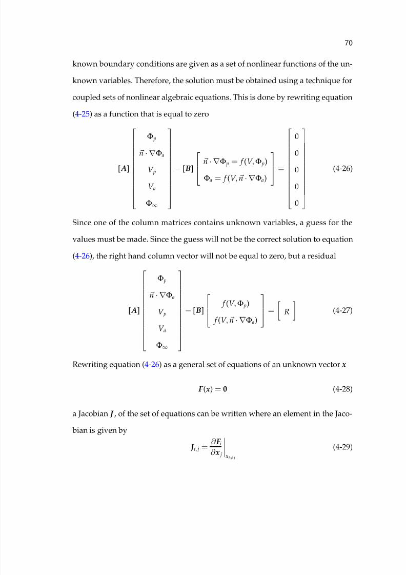
7/18/2019 Riemer PhD 2000


70

known boundary conditions are given as a set of nonlinear functions of the un-

known variables. Therefore, the solution must be obtained using a technique for

coupled sets of nonlinear algebraic equations. This is done by rewriting equation(4-25) as a function that is equal to zero

[ A]

Φ p

n · ∇Φa

V p

V a

Φ∞

− [B]

n · ∇Φ p = f (V ,Φ p)

Φa = f (V , n · ∇Φa)

=

0

0

0

0

0

(4-26)

Since one of the column matrices contains unknown variables, a guess for the

values must be made. Since the guess will not be the correct solution to equation

(4-26), the right hand column vector will not be equal to zero, but a residual

[ A]

Φ p

n

· ∇Φa

V p

V a

Φ∞

− [B]

f (V ,Φ p)

f (V , n · ∇Φa)

= R

(4-27)

Rewriting equation (4-26) as a general set of equations of an unknown vector x

F ( x) = 0 (4-28)

a Jacobian J , of the set of equations can be written where an element in the Jaco-

bian is given by

J i, j =∂ F i∂ x j

x= j

(4-29)

7/18/2019 Riemer PhD 2000


71

Then the Newton-Raphson iteration can be performed as in section 4.5 on

page 62 to obtain the solution vector x such that equation (4-28) holds. Again the

line search is necessary for the the method to work. However, in most non-trivialcases, even the line searches fail.

In order to get the method to converge to a solution, many techniques were

tried including the minimal residual techniques such as the modified Powell

method,73 Levenberg-Marquort techniques and other methods such as the conju-

gate gradient method. These techniques would converge sometimes if the guess

was nearly the correct value.

4.9 Variable Transformation to Stabilize Convergence

The system of equation that result from Φ, V , i as the set of variables for the

solution has very poor convergence characteristics. Great effort was required

to bring the system to convergence. Standard line searches and even minimal

residual techniques failed to converge.

A simple variable transformation has been developed that enables good con-

vergence properties using the simple line search method. The variable transfor-

mation needed can be seen easily from the equations used to describe the kinetics

i = 10V −Φ−EFe

β Fe −

1

ilim,O2

+ 10

V −Φ−EO2β O2

−1

10− V −Φ−EH2

β H2 (4-30)

In equation (4-30), the difference V −Φ appears many times. A simple transfor-

mation can be written

Ψ= V −Φ (4-31)

7/18/2019 Riemer PhD 2000


72

where Ψ represents the driving force for the electrochemical kinetics. The vari-

able V is then chosen as the dependent variable and rewritten as

V =Ψ+Φ (4-32)

All of the equations used for the kinetics, bare metal (1-23), coated metal (1-26),

galvanic anodes (1-27), and impressed current anodes (1-30) can be rewritten in

terms of the new variable. For bare metal, one obtains

i = 10Ψ−EFe

β Fe −

1

ilim,O2

+ 10

Ψ−EO2β O2

−1

10−Ψ−EH2

β H2 (4-33)

for coated metal there are two simultaneous equations in two unknowns that

describe the current density

i =− (Φ−Φin)

ρfilmδ film(4-34)

and

i = Apore

A10

Ψ+Φ−Φin−EFeβ Fe

− 1

(1 − α block) ilim,O2 −10

Ψ+Φ−Φin−EO2β O2

−1

−10

−(Ψ+Φ−Φin−EH2 )β H2

(4-35)

for galvanic anodes

Ψ= Eanode + β anode log(i/icorr + 1) (4-36)

and finally for impressed current anodes

Ψ=

V

rectifier+ E

O2

+ β O2

log(i/icorr

+ 1) (4-37)

where V rectifier is the known setting for the rectifier.

The set of equations for the finite element method must also be rewritten as

K [Ψ+Φ] = f

(4-38)

7/18/2019 Riemer PhD 2000


73

where f and K do not change. The boundary element method is not changed.

The set of equations that is solved becomes:

0 0 H p, p H a, p −4π

0 0 H p,a H a,a −4π

K p 0 K p 0 0

0 K a 0 K a 0

0 0 0 0 0

Ψ p

Ψa

Φ p

Φa

Φ∞

=

G p, p Ga, p

G p,a Ga,a

ˆ F p 0

0 ˆ F a

A p Aa

n · ∇Φ p

n · ∇Φa

(4-39)

At this point the essential boundary condition for V (Ψ+Φ) is applied. There is

one degree of freedom in the problem for this potential so one node on one pipe

is selected to have a 0 potential. This is done be replacing the FEM equation for

the single selected node in the system given by equation (4-39) with the equation

Ψ+Φ= 0 (4-40)

The FEM equation (lower half of the system) is replaced because that is where the

degree of freedom in the reference potential is. If there are multiple CP systems,then there must be an equal number of essential boundary conditions on Ψ+Φ.

Once the equations are set up, all unknown variables are placed on the left-hand-

side, which are Φ and Ψ for cathodes (pipes, tank bottoms, ship hulls, etc.) and

n · ∇Φ and Φ for anodes. The reordered system of equations is

0 −Ga, p H p, p H a, p −4π

0 −Ga,a H p,a H a,a −4π K p 0 K p 0 0

0 − ˆ F a 0 K a 0

0 − Aa 0 0 0

Ψ p

n · ∇Φa

Φ p

Φa

Φ∞

=

G p, p 0

G p,a 0ˆ F p 0

0 − K a A p 0

n · ∇Φ p

Ψa

(4-41)

7/18/2019 Riemer PhD 2000


74

The above system of equations is then solved using the same technique as de-

scribed in section 4.5. This system has excellent convergence characteristics and

uses about the same number of iterations as the method without attenuation.

4.10 Conclusions

A method has been developed to model cathodic protection of complicated

pipeline networks. It utilizes the boundary element method to solve Laplac’s

equation within the soil and it accounts for the non-zero voltage drop in long

pipes using a finite element solution.

A new variable transformation has been described to stabilize the conver-

gence of the application of the nonlinear boundary conditions.

There are still some issues to be dealt with in the development of a working

model. The creation of an optimized mesh is treated in the next chapter. Verifica-

tion of the solution techniques is done in Chapter 7.

7/18/2019 Riemer PhD 2000


CHAPTER 5MESH GENERATION

Figure 5-1: Type of mesh needed for model. Three pipes are shown passingthrough a point where the soil conductivity changes.

The Boundary Element Method (BEM) and the Finite Element Method (FEM)

rely on a mesh in order to solve the differential equations. A mesh is a set of

lines, triangles, rectangles or other shapes that when pieced together, form the

boundaries of the geometry of interest. The finite element method also must have

the domain enclosed by the boundaries divided up into these shapes. The BEM

needs a mesh on the boundaries only. These shapes are called elements hence the

name of the numerical methods.

Elements use a shape function to approximate the solution along the geom-

etry described by the element. The number of elements should be sufficient to

75

7/18/2019 Riemer PhD 2000


76

allow the shape functions to approximate the solution to the governing differen-

tial equation.

One of the most difficult problems to address in computer code is how to dis-cretize an object such that the solution obtained from the BEM and FEM contains

a desired minimum level of information. For a discretization method to succeed,

it must not only be able to describe the solution accurately, but must also describe

the geometry sufficiently well so that the solution can be obtained.

5.1 Basic Mesh

The basic mesh must account for the current and potential distribution both

axially and around the circumference of the pipe. It is accomplished be divid-

ing the pipe surface (boundary to the soil domain) into 2-dimensional elements

that are piece-wise continuous. The elements are not planar. They are wrapped

onto the pipe geometry like wrapping paper to a gift. Therefore the elements

are 2-dimensional only in a curvi-linear coordinate system. A coordinate trans-

formation must be derived to map the 2-dimensional curvi-linear system to the

3-dimensional cartesian system where the differential equation is solved. In the

curvi-linear system, the element is called the parent element since all the elements

have the same size and shape in that system.

5.1.1 Discretization and Shape Functions

The family of elements that use the same basis (shape) functions to describe

the geometry over the surface of the element as well as the solution to the dif-

ferential equation over the element are called iso-parametric elements.67, 74 These

7/18/2019 Riemer PhD 2000


77

Figure 5-2: Circle discretized with 8 linear triangular elements. The area is 2√

2r2

for the 8 triangles which is a 10.% error.

elements have been used in the code that has been developed. The choice of el-

ement shape has been dictated by the geometry being represented. The element

that best fits the sides of a cylinder is a quadrilateral element while triangles are

best used on the ends. The only remaining issue then is to choose how manynodes and therefore the order of the basis polynomials used to describe the vari-

ation of the geometry and solution over the individual elements.

Basis functions considered for the elements were: 1) constant, 2) linear, 3)

quadratic, and 4) cubic. Of these, the curved functions, quadratic and higher,

make the most sense because of the curvature of the geometry. They also make

sense for representing the solution since they can more easily describe the curve

heading into the singularity in the current density that occurs at junctions be-

tween different boundary conditions where the angle of the geometry at the junc-

tion is not 90 degrees. Table 5.1 shows the capability of 3 types of elements to rep-

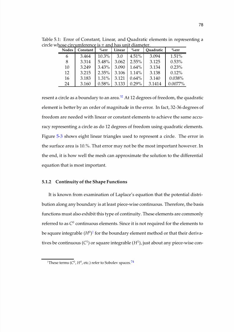
7/18/2019 Riemer PhD 2000


78

Table 5.1: Error of Constant, Linear, and Quadratic elements in representing acircle whose circumference is π and has unit diameter.

Nodes Constant %err Linear %err Quadratic %err

6 3.464 10.3% 3.0 4.51% 3.094 1.51%8 3.314 5.48% 3.062 2.55% 3.125 0.53%10 3.249 3.43% 3.090 1.64% 3.134 0.23%12 3.215 2.35% 3.106 1.14% 3.138 0.12%16 3.183 1.31% 3.121 0.64% 3.140 0.038%24 3.160 0.58% 3.133 0.29% 3.1414 0.0077%

resent a circle as a boundary to an area.32 At 12 degrees of freedom, the quadratic

element is better by an order of magnitude in the error. In fact, 32-36 degrees of

freedom are needed with linear or constant elements to achieve the same accu-

racy representing a circle as do 12 degrees of freedom using quadratic elements.

Figure 5-3 shows eight linear triangles used to represent a circle. The error in

the surface area is 10.%. That error may not be the most important however. In

the end, it is how well the mesh can approximate the solution to the differential

equation that is most important.

5.1.2 Continuity of the Shape Functions

It is known from examination of Laplace’s equation that the potential distri-

bution along any boundary is at least piece-wise continuous. Therefore, the basis

functions must also exhibit this type of continuity. These elements are commonly

referred to as C0 continuous elements. Since it is not required for the elements to

be square integrable ( H 0)† for the boundary element method or that their deriva-

tives be continuous (C1) or square integrable ( H 1), just about any piece-wise con-

†These terms (C0, H 0, etc.) refer to Sobolev spaces.74

7/18/2019 Riemer PhD 2000


79

1 0.8 0.6 0.4 0.2 0 0.2 0.4 0.6 0.8 11

0.8

0.6

0.4

0.2

0

0.2

0.4

0.6

0.8

1

Figure 5-3: Four quadratic elements with eight degrees of freedom representinga circle.

7/18/2019 Riemer PhD 2000


80

0 10

20 30

40 50

0

10

20

0

0.5

1

Figure 5-4: Continuity of the basis functions. Two elements are shown. Basisfunctions that share a node with a value of one must be continuous.

tinuous function could be used as the basis functions. However, the finite ele-

ment method used within the steel of the pipe must use square integrable ( H 0)

shape functions.74 It is also necessary to have the solutions between the soil and

steel match up. Therefore the same element needs to be used in both numerical

methods. Lagrange polynomial basis functions are very well developed in the

literature,67, 74 and are often needed for boundary element methods.63 They work

well for FEM, so they are used when rectangular shapes are needed such as the

walls of the pipe. In the case of this code, quadratic Lagrangian iso-parametric

elements are used which exhibit the necessary quality of H 0 continuity.

It is often required to include triangular elements to properly describe the

geometry. The triangles must be piece-wise continuous and be continuous with

any rectangular elements they may be in contact with. Quadratic iso-parametric

triangles are used for this purpose. They exhibit C0 continuity with the Lagragian

type elements. The triangles can then be used to increase or decrease the local

7/18/2019 Riemer PhD 2000


81

Figure 5-5: Use of triangles to increase the degrees of freedom in the center region

while maintaining C0

continuity.67

density of nodes while maintaining continuity throughout the boundary. They

can also be used to describe difficult shapes such as coating holidays, ends of

pipes, and tank bottoms. Figure 5-5 shows how triangular elements can be used

to increase the density of elements in a small region. Small regions occur any

time a holiday is placed on the pipe.

5.1.3 Quadratic Iso-Parametric Rectangles

Quadratic Lagrangian iso-parametric rectangular elements are used for most

of the mesh that constitutes the pipes and anodes. The parent element contains 9

nodes and nine shapes functions. The geometry and solution is written in terms

of the shape functions, i.e.

u(η, ξ ) =9

∑i=1

φi(η, ξ )ui (5-1)

where φ i is the shape function and η and ξ are homogeneous coordinates in the

parent element that take values from -1 to 1, u is the quantity of interest such as

7/18/2019 Riemer PhD 2000


82

ξ

η

1 2 3

4 5 6

7 8 9

Figure 5-6: Quadratic iso-parametric rectangular parent element. Numbering of nodes and shape functions given in figure.

the x coordinate or the solution to the differential equation, and ui is the value of

the quantity of interest at node i. The nodes are numbered as in Figure 5-6. The

shape functions corresponding to each node are given respectively

φ1 =1

4

η(η

−1)ξ (ξ

−1) (5-2)

φ2 =1

2(1 − η2)ξ (ξ − 1) (5-3)

φ3 =1

4η(1+ η)ξ (ξ − 1) (5-4)

φ4 =1

2η(η − 1)(1 − ξ 2) (5-5)

φ5 = (1 − η2)(1 − ξ 2) (5-6)

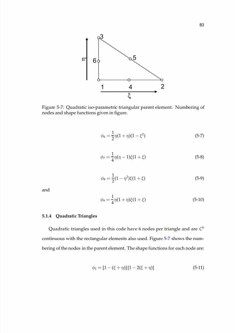
7/18/2019 Riemer PhD 2000


83

1 4 2

5

3

6

ξ

η

Figure 5-7: Quadratic iso-parametric triangular parent element. Numbering of nodes and shape functions given in figure.

φ6 =1

2η(1+ η)(1 − ξ 2) (5-7)

φ7 =1

4η(η − 1)ξ (1+ ξ ) (5-8)

φ8 =12

(1 − η2)ξ (1+ ξ ) (5-9)

and

φ9 =1

4η(1+ η)ξ (1+ ξ ) (5-10)

5.1.4 Quadratic Triangles

Quadratic triangles used in this code have 6 nodes per triangle and are C0

continuous with the rectangular elements also used. Figure 5-7 shows the num-

bering of the nodes in the parent element. The shape functions for each node are:

φ1 = [1 − (ξ + η)] [1 − 2(ξ + η)] (5-11)

7/18/2019 Riemer PhD 2000


84

φ2 = ξ (2ξ − 1) (5-12)

φ3 = η(2η − 1) (5-13)

φ4 = 4ξ [1 − (ξ + η)] (5-14)

φ5 = 4ξη (5-15)

and

φ6 = 4η [1 − (ξ + η)] (5-16)

5.2 Long Pipes

Long pipes must be meshed with a minimum number of nodes, yet account

for the nature of the solution. If elements of an aspect ratio of one are used to

create the mesh for the entire pipe, only very short sections of pipe could be

modeled before memory limitations of the computer would be exceeded. There-

fore, the aspect ratio of any element cannot be restricted to something near one.

In fact, the aspect ratios need to be as large as 5000 to 1 (length to width) to model

the complete potential and current distributions for long pipes with the limited

resources available on a PC (October, 2000 - 1GB RAM). However, there are se-

vere numerical difficulties encountered with elements of these aspect ratios. The

solution to these problems is addressed in section 6.2.

High aspect-ratio elements cannot be used at the ends of the pipe or where

there is a change in the nature of the boundary condition i.e., a change in the

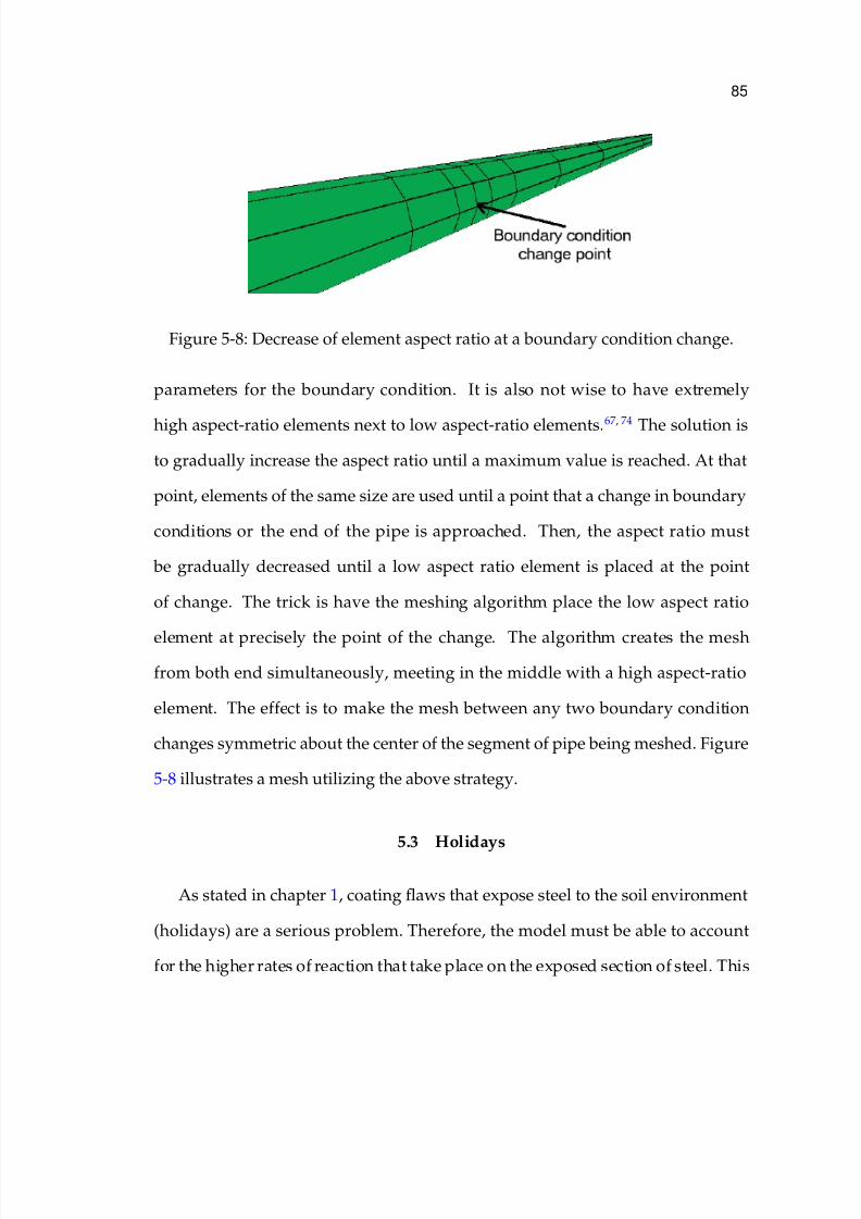
7/18/2019 Riemer PhD 2000


85

Figure 5-8: Decrease of element aspect ratio at a boundary condition change.

parameters for the boundary condition. It is also not wise to have extremely

high aspect-ratio elements next to low aspect-ratio elements.67, 74

The solution is

to gradually increase the aspect ratio until a maximum value is reached. At that

point, elements of the same size are used until a point that a change in boundary

conditions or the end of the pipe is approached. Then, the aspect ratio must

be gradually decreased until a low aspect ratio element is placed at the point

of change. The trick is have the meshing algorithm place the low aspect ratio

element at precisely the point of the change. The algorithm creates the mesh

from both end simultaneously, meeting in the middle with a high aspect-ratio

element. The effect is to make the mesh between any two boundary condition

changes symmetric about the center of the segment of pipe being meshed. Figure

5-8 illustrates a mesh utilizing the above strategy.

5.3 Holidays

As stated in chapter 1, coating flaws that expose steel to the soil environment

(holidays) are a serious problem. Therefore, the model must be able to account

for the higher rates of reaction that take place on the exposed section of steel. This

7/18/2019 Riemer PhD 2000


86

is done through the kinetic expressions used as the boundary conditions. Since

any individual element must have the same boundary condition expression, the

mesh must provide entire elements that define the size and location of a holiday.Also, when using second order polynomials to describe the solution over any

individual element, more than one element is needed on the holiday to account

properly for the nonuniform current distribution. The sample calculations pre-

sented in Figure 5-9 illustrate the need for refined meshing of coating holidays.

For even small values of J = −αc Froiavg/RT κ, a single second order polynomial

cannot adequately represent the solution. Therefore, the diameter of the holidayneeds at least two quadratic elements for small values of J and four or more for

larger values.

Holidays are meshed is two possible ways. If the holiday is round, it is easiest

to use a constrained Dalauny mesh generator.75, 76 If the holiday is not round such

as a gouge in the coating due to mechanical damage, a different approach uses

rectangular elements is used.

5.3.1 Round Holidays

For the this model, the method that was used to generate a Dalauny mesh

comes from Jonathan Richard Shewchuck.77 The code is publically available with

documentation (October, 2000).78 The generator takes an input of a planar straight

line graph (PSLG). It then creates a mesh of linear or quadratic triangles that

conform to the mesh.

The generator is included as a black-box library function in the program. The

author of the code provided a simple interface to the generator that utilized the

7/18/2019 Riemer PhD 2000


87

0

0.2

0.4

0.6

0.8

1

1.2

1.4

1.6

1.8

0 0.2 0.4 0.6 0.8 1

r/r o

i / i a v g

J=1.92

J=3.30

J=4.88J=0.35

J=-αcFr oiavg/RTκ

Figure 5-9: Current density distribution on a circular holiday. Parameter J is afunction of the average current density iavg, the inverse Tafel slope αc F

RT , the holiday

radius ro, and the soil resistivity κ.

7/18/2019 Riemer PhD 2000


88

Figure 5-10: A mesh that includes two round holidays. This is the output froma standard mesh generator.77 Further processing is needed to map the mesh to apipe and adjust the holidays so they are round.

same command line options as the stand-alone code. The PSLG input is created

as the boundary to the region being divided into elements. This is usually a

rectangle, a circle, or a half circle which are trivial to create and a list of holes

(holidays) that must be included. The output is then the mesh created by the

library.

The output of the generator is not ideally suited for for a pipe. The code gen-

erates a mesh that is on a 2-dimensional plane as in Figure 5-10. The mesh must

then be post-processed in order to have all the desired properties. The holidays

are dealt with first. The output along the edge of the holiday is a piece-wise set of

straight lines. Since the elements are quadratic in nature, a better job can be done

by moving the center node of each line segment onto the circle used to define the

holiday. As seen in Figure 5-3, the quadratic nature of each side of the element

can be utilized to more closely follow the correct geometry.

7/18/2019 Riemer PhD 2000


89

Figure 5-11: The same mesh as shown in Figure 5-10. Here the elements for theholiday have been removed. The elements have been divided into four trianglesto illustrate the locations of the center nodes on each side of the triangles.

Figure 5-11 shows the locations of the center nodes on each side of an ele-

ment by subdividing each element up into four smaller elements using the center

nodes. Segments of the holiday boundary are seen to bee straight lines consist-

ing of two segments. After the nodes at the center of the lines are moved to their

proper positions, the circle is defined as best that can be done with a fixed number

of quadratic line segments see Figure 5-12. The movement can be done so long

as the angle at any corner of the triangle is greater than 0 degrees. In fact, it is de-

sirable to have the angles of all the corners of the elements be greater than about

15 degrees.67 This avoids numerical difficulties with large aspect ratio triangles

when blind Gaussian integration is used. The problem is greatly alleviated using

integration techniques described in section 6.2.

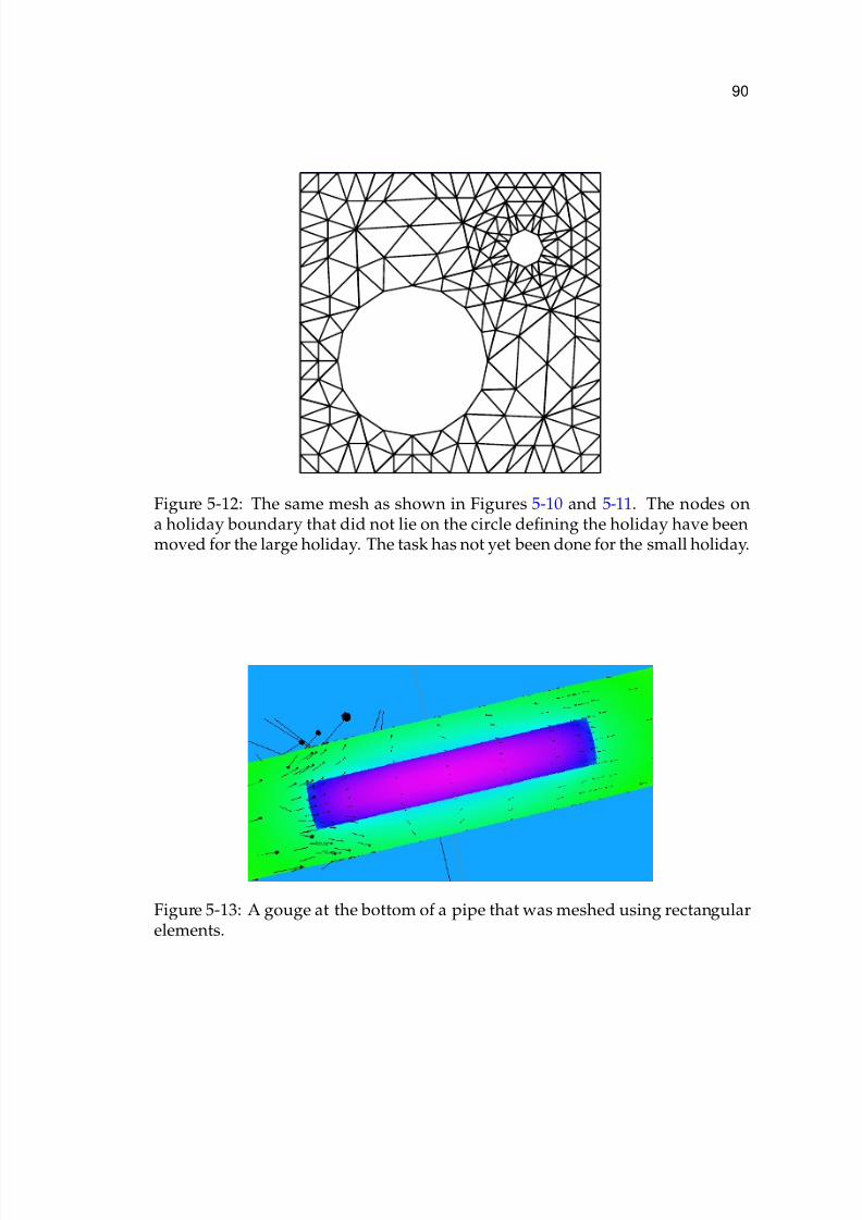
7/18/2019 Riemer PhD 2000


90

Figure 5-12: The same mesh as shown in Figures 5-10 and 5-11. The nodes ona holiday boundary that did not lie on the circle defining the holiday have beenmoved for the large holiday. The task has not yet been done for the small holiday.

Figure 5-13: A gouge at the bottom of a pipe that was meshed using rectangularelements.

7/18/2019 Riemer PhD 2000


91

Figure 5-14: Closeup of one edge of a rectangular holiday where two triangleshave been used to increase the element density of the holiday.

5.3.2 Rectangular Holidays

Rectangular holidays such as a gouge, use a different mesh technique. In

order to adequately approximate the current and potential distribution across

the gouge, three elements are needed. Along the length of the gouge, a minimum

of three elements would be needed. Because the shape of a gouge is roughly

rectangular, it is best to use the rectangular elements to create the mesh. In this

case triangular elements are used to increase the element density at the holiday as

described in section 5.1.2. Two triangles are placed at either end of the holiday to

increase the number of elements across the holiday from one to three. See Figure

5-14 for details of the arrangement.

There are a number of problems placing holidays on the pipe. For both mesh-

ing practices described, there can be some distortion of the pipe surface due to

wrapping the planar elements to the pipe. It is most often seen as a ripple in the

surface near the edge of the holiday. Great effort has been made to minimize the

7/18/2019 Riemer PhD 2000


92

unwanted effect, but if too few nodes are specified to mesh the circumference of

the pipe, the problem is exacerbated.

5.4 Pipe Crossings and Shadowing

When two pipes cross, attention must be paid to the nature of the mesh gen-

erated. Both pipes must account for, in their solution, the effect of the close ap-

proach of the other pipe. Pipeline operating companies can attest to the fact that

the pipes will greatly interfere with each other and that special precautions are

needed.

In order to account for the close approach of another pipe in the solution,

the mesh must be adjusted. There must be sufficient nodes located at the point of

closest approach, but too many nodes is a waste of computer time. For simplicity,

the same technique used for a change in coating properties is used. At the point

of crossing, a coating property change in placed to force the mesh generator to in-

crease the element density at that point, see Figure 5-15. With the addition of the

extra elements, the model has the flexibility in the solution to closely approximate

the solution at the crossing.

5.5 Soil Type Divisions

The boundary element method must have the boundary of changes in bulk

properties meshed. For applications to pipelines contained in semi-infinite do-

mains, the boundary that is to be divided into elements extends to infinity. Mesh

generators cannot create a mesh that extends to infinity with standard elements.

Therefore, a mesh is created that extends sufficiently far into the domain such

7/18/2019 Riemer PhD 2000


93

Figure 5-15: Mesh at a crossing of two pipes. Both pipes have the highest densityof elements at the crossing point.

that most of the variations in potential and current density have died out. At the

end of this mesh, a special element known as an infinite element is placed. The

classic definitions for infinite elements are given by Beer.79

Soil divisions may need to have holes in the mesh to allow pipes the passthrough. Since the location and number of pipes is arbitrary, the same mesh

generator used to create holidays is used.77 Sample output of the mesh generator

is shown in Figure 5-16.

Pipes are added to the mesh such that the nodes of the pipe at the point of

crossing the soil type division, match exactly the nodes at the edges of the holes

in the division. A completed mesh with pipes is shown in Figure 5-17.

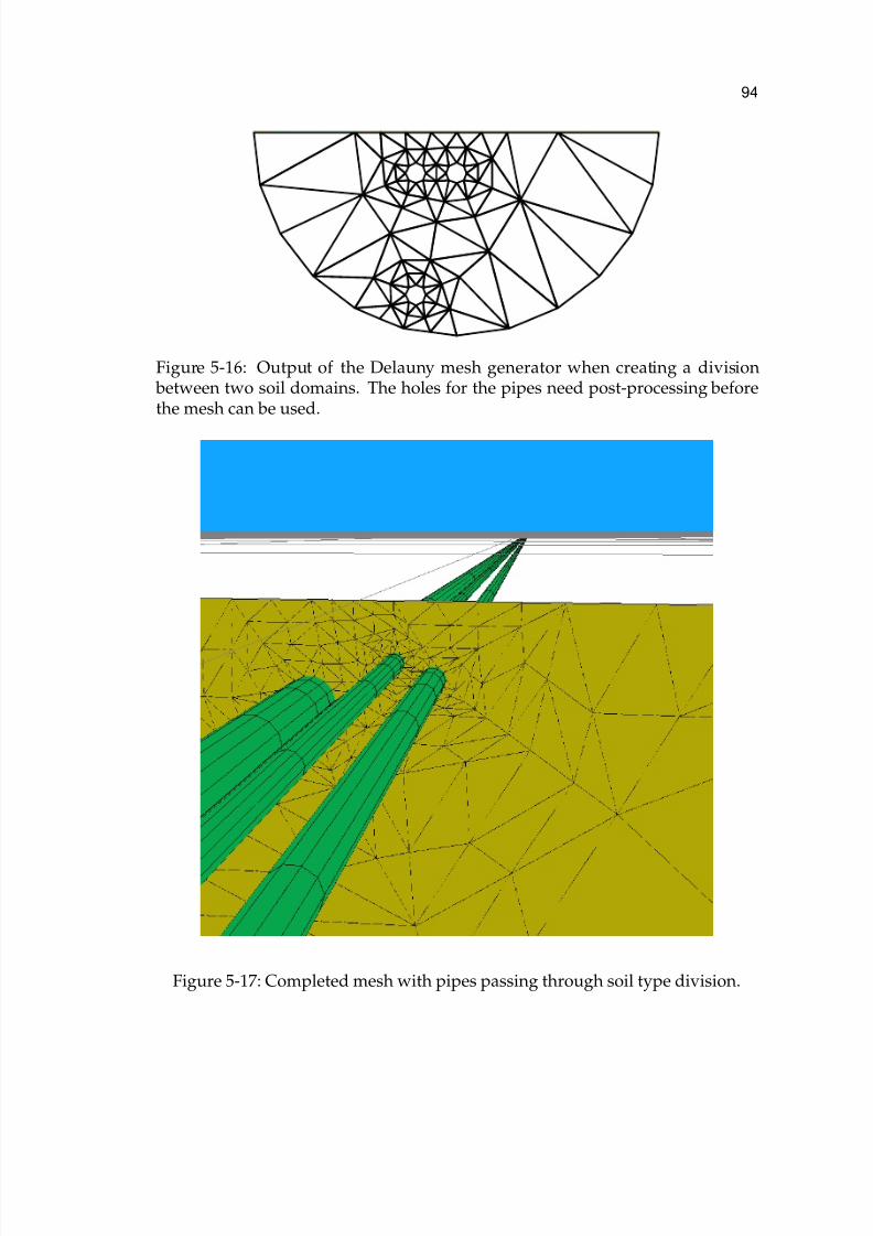
7/18/2019 Riemer PhD 2000


94

Figure 5-16: Output of the Delauny mesh generator when creating a division between two soil domains. The holes for the pipes need post-processing beforethe mesh can be used.

Figure 5-17: Completed mesh with pipes passing through soil type division.

7/18/2019 Riemer PhD 2000


95

5.6 Conclusions

The generation of the boundary element and finite element mesh is a critical

component for the solution of the differential equations describing cathodic pro-

tection of pipelines. The solution obtained form the BEM and FEM can only be

trusted if the underlying mesh is of sufficient quality such that the shape func-

tions can closely approximate the true solution. The next two chapter discuss

how errors using the type of mesh described in this chapter can be reduced and

how the solution has been verified.

7/18/2019 Riemer PhD 2000


CHAPTER 6SOLUTION ACCURACY

There are a great many factors that affect the accuracy of a solution obtained

by the Boundary Element Method. These include the basis (shape) functions used

to approximate the solution on the finite element, the size and location of an

element, and the numerical method used to evaluate the integrals seen in the

method - equation (3-9) in the Chapter 2 on page 32.

6.1 Sources of Error

Errors in the boundary element method come from several sources. They can

be discretization, integration,80, 81, 82, 83, 84, 85, 86 shape function choice, and matrix

inversions. Of these, discretization and integration can be the largest source of

error if not handled carefully.

Discretization presents a tricky balance between minimizing the size of the

matrices and having elements whose shape function adequately approximates

the solution to the PDE on the element for which it is applied. Choosing a shape

function - element size pair that cannot represent the solution to a given error

level can greatly affect the solution throughout the domain. This is because the

boundary element method applied to any given point in the domain or on the

boundary is a function of all the points on the boundary, including the point

itself if it is on the boundary.

96

7/18/2019 Riemer PhD 2000


97

Another source of error is representing the discontinuity in the derivative at

junctions between different boundary conditions. This error can be conveniently

eliminated if one is willing to expand the size of one the matrices.62

Integration presents one of the most difficult and time consuming aspects of

the Boundary Element Method. There have been many papers devoted to eas-

ing the difficulty and improving the accuracy of the results.80, 81, 82, 83, 84, 85, 86, 87, 88, 89

The reason for this is that the integration kernel (in 3D) contains a weak singu-

larity (1/r) and a strong singularity (1/r2) which must be evaluated in a Cauchy

principle value sense.

6.2 Integration Accuracy

Since the kernel is not a polynomial, a Gaussian integration scheme cannot

be found to evaluate it exactly. However, early implementations of BEM sim-

ply used a basic Gaussian quadrature to evaluate the singular integrals.82 After

recognizing that the results of the integrals were the major source of error, sev-

eral techniques have been utilized to remove the singularity. For simple shape

functions and elements, a transformation to polar coordinates on the boundaries

may be used to evaluate the weakly singular integrals.81, 82 However, the strongly

singular integrals cannot be evaluated easily. All of the strongly singular inte-

grals are located on the diagonal of the H matrix (see section 4.1.1 for details of

this matrix). For these integrals there are two choices if the physics of the prob-

lem warrant. The first and easiest is to make use of a unit displacement or a

constant potential distribution solution which is due to Gibbs.68 If the body is

not elasto-plastic in nature (mechanics) or does not store charge in the domain

7/18/2019 Riemer PhD 2000


98

(steady-state), then the solution to the normal flux at the boundary is known to

be zero. This gives the equation

H I = 0 (6-1)

where I is a column matrix all of whose elements are 1’s. Then the unknown

strongly singular integral, of which there is only 1 per row, can be solved explic-

itly by the equation

H i,i =∑ j=i

H i, j (6-2)

The second technique is to solve the Cauchy principle value explicitly. There are

techniques for doing this for the direct boundary element method described by

Guiggianni 83, 84 and for the Symmetric Galerkin Boundary Element Method by

the same author. 90

6.3 Integration Techniques

There are several ways to improve the accuracy of a given integral over an

arbitrary element. The easiest is to increase the order of the Gaussian quadrature.

This technique though, can never integrate a weakly singular integral since it

cannot be represented as a finite order polynomial.

Two dimensional Gaussian quadrature can be used to speed up the calcula-

tions significantly. Cools et al.91 have made available general integration source

code for a variety of two-dimensional shapes. They term two-dimensional Gauss

rules as “Cubature.”

Singular integrals can benefit from a change of the coordinate system to polar

coordinates. Polar coordinates reduce the order of the singularity by one. For

7/18/2019 Riemer PhD 2000


99

the 1/r dependence of the G integral, the singularity is removed as well as all

dependence on 1/r as one approaches the singularity. For the 1/r2 dependence

of the H integral, it is now possible to get a rapidly converging result.

6.3.1 Adaptive Integration

The final choice made for this project was to use a specially modified form

of a two dimensional cubature rewritten for an adaptive scheme. The possibility

of having extremely large aspect ratios in the elements to be integrated required

modifications of published integration subroutines. This also meant that stan-dard routines like IMSL could not be used.92 The routines that are used are based

on a 1-dimensional algorithm93 distributed by NIST at.94 The routine was mod-

ified to solve 2-D integrals by using Gauss-Kronrod cubature formula95 and to

take into account the high aspect ratios. The modified subroutine takes any arbi-

trary triangle and seeks to subdivide it such that the subdivisions are performed

in the area with the largest error contribution to the total error for that element. Italso tries to extrapolate the subdivisions with a nonlinear algorithm to reduce the

amount of computational time. The Gauss-Kronrod 2-D integration rules provide

a value for the integral over a certain specified geometric shape and an estimate

of the error in the integration. This is accomplished by actually having two inte-

gration rules of different order, where the higher order formula is a super-set of

the other. This means that for a 13-15 rule, 13 points form the lower order rule

and the addition of only two more points to the rule gives the 15 point formula.

It is computationally cheap because the first 13 points of the 15 point rule are

identical to the 13 point rule. Adapting the integration routine for high aspect

7/18/2019 Riemer PhD 2000


100

Section 1 Section 2

Figure 6-1: Sub-element with a high aspect ratio subdivided by the adaptive in-tegration routine to reduce the aspect ratio of the subsections.

Section 1 Section 2

Section 3 Section 4

Figure 6-2: Sub-element with a desired aspect ratio subdivided by the adaptiveintegration routine.

ratio elements is very straight forward. After finding the subsection that has the

largest error contribution, the aspect ratio of the real sub-element is calculated.

If the ratio is greater than 2 or less than 0.5, the element is divided into two sub-

sections such that the aspect ratio of the sub-sections is reduced (or enlarged) to

bring it closer to the desired range. If the aspect ratio is already within the desired

range, the section is sub-divided into 4 sub-sections.

By implementing the modifications to the adaptive integration routine based

on the aspect ratio of the sub-sections, a order-of -magnitude performance im-

provement was achieved while maintaining the same accuracy.

A new technique has been introduced by Karafiat that could reduce the time

to complete the integration by another order of magnitude.89 This method moves

7/18/2019 Riemer PhD 2000


101

the vertices of a small number of sub-triangles to optimize the effect of the quadra-

ture. However, there is some ambiguity in the cost function that places these

nodes, in that a local minimum can be found without obtaining the global mini-mum. Also, the technique was only described for a case where the singularity lies

in the same transformed plane as the element itself. For 3D models of pipelines,

the singularity may be located anywhere (i.e. above the center of the element) in

which case the algorithm fails.

6.3.2 Singular Integrals

Singular integrals are handled by first insuring that the point of singularity

is at a vertex. This is done by breaking the domain of integration manually into

several subsections such that the singularity is on a desirable vertex. Second, it is

important for accuracy that the subsections that actually contain the singularity

have an aspect ratio of 1.0. For instance, suppose a quadratic Lagrangian element

is to be integrated, and the singularity is at the lower left corner. The element isthen broken into 3 separate integration domains. One that contains the singular-

ity and two the are “nearly singular” because of the proximity of the singularity.

The subsection with the singularity is integrated in polar coordinates to reduce

the order of the singularity, while the other two subsections are integrated using

the standard adaptive integration.

6.4 Matrix Inversions

The solution of Ax = b is another source of error. For large systems of equa-

tions, Gaussian elimination is a very poor choice on computers. The reason for

7/18/2019 Riemer PhD 2000


102

this is the enormous propagation of round-off errors in the solution column b.

Every division used in Gaussian elimination increases the error of a particular

element. That error is added to every other element in the column through therow operation used to eliminate elements in the matrix A. This is repeated during

back-substitution which carries the error back up through the column to elements

which might have a lower contribution from round-off error.

LU decomposition can reduce the error to a reasonable level. This is because

of the significant reduction of round-off error of the b vector. The implementa-

tion used in the code is a standard subroutine from LAPACK named dgesv andits dependencies.96 This subroutine makes extensive use of BLAS (Basic Linear

Algebra Subroutines).97 The source code for these libraries can be found on the

world-wide-web at the locations given in the references. These subroutines can

be linked together to perform almost any type of linear algebra function. There

is an added benefit in that the BLAS routines have been highly optimized for al-

most all computing platforms and are freely available. The optimized versions

can have a performance impact of 2 to 16 over just compiling the basic source

code. The libraries for Intel processors running a Win32 operating system can

also be obtained on the world-wide-web.98 At the time of this writing (October,

2000), Intel had not posted the libraries for the Linux/FreeBSD environments yet

although beta versions were available for testers.

7/18/2019 Riemer PhD 2000


CHAPTER 7MODEL VERIFICATION

After the code has been written to solve a differential equation, it is important

to benchmark it against known solutions. The code used herein solves Laplace’s

equation in a half space. There are two analytic solutions to Laplaces equation

for a half space that have been used to verify different portion of the code. The

first is due to Newman where a disk electrode is placed on the plane defining a

half-space and the primary current distribution is found. This solution provides a

test on the quality of the solution to Laplace’s equation.99 It contains a singularity

in the solution that causes the current density at the edge of the disk to approach

infinity. Most numerical solutions have a great deal of difficulty obtaining this

solution.

The second analytic solution is due to Kasper.8 This solution is directly rele-

vant to pipes because it solves Laplace’s equation for two parallel infinitely long

cylinders. This solution shows the importance of the solution around the cir-

cumference of the pipe and can give an indication of the “fineness” of the mesh

needed around the circumference of the pipe.

A third related solution is from Dwight.3 His equation is used to find the re-

sistance between a metal electrode and a point at infinity. It assumes constant

potential along the entire surface of the electrode.

103

7/18/2019 Riemer PhD 2000


104

7.1 Primary Current Distribution to a Disk

Newman’s solution to Laplace’s equation for the primary current distribution

of a disk electrode in a half-space containing and a counter-electrode at a great

distance away is given by99

i

iavg=

0.5 1+ (r/ro)2

(7-1)

where ro is the radius of the disk, i is the current density at a distance r from

the center of the disk and iavg is the average current density for the entire disk.

The disk is placed on the plane that defines the half-space. The counter-electrode

must be at a great distance so that it does not interfere with the current distri-

bution. It also should have a greater surface area than the electrode so that the

ohmic control is at the electrode.

7.1.1 Disk in a Half Space

The first comparison to the analytic solution given in equation (7-1) is for a

model setup that is nearly identical to that used in obtaining equation (7-1). The

model setup is shown in Figure 7-1. The model used a disk of 15.24 meters diam-

eter. The anode was placed 500 meters from the disk. Hydrogen evolution Tafel

kinetics were used for the boundary condition. At a sufficient current level, the

distribution should approach the primary distribution given by equation (7-1).12

For hydrogen evolution, the numerical calculation approached the primary dis-

tribution when the average current density was about 0.75µA/cm2. The results of

the calculation and the analytic solution are plotted together in Figure 7-2, where

the solid line represents the analytic solution. The results show excellent agree-

7/18/2019 Riemer PhD 2000


105

Figure 7-1: Primary current distribution on a disk electrode in a half-plane.Model solution at center of disk is within 2.0% of the analytic solution of i/iavg =

0.5. This view is looking along the z axis toward the disk.

0.1

1

10

0.001 0.01 0.1 1

1-r/r o

i / i a v g

Figure 7-2: Comparison of primary current distribution on a disk electrode ina half-plane. Red line without circles is the analytic solution, blue line is thenumerical solution from the disk shown in Figure 7-1.

7/18/2019 Riemer PhD 2000


106

Figure 7-3: Disk holiday on a pipe. Shading corresponds to the off-potential.Note the draw-down of potential in the coated region around the holiday.

ment with the analytic solution over all but the edge of the disk. The difficulty at

the edge is that a numerical method cannot approximate infinity very well. When

the solution is placed on a log-log plot, a straight line should be seen as 1 − r/ro

approaches zero. A good approximation to the straight line is made when the the

mesh is sufficiently fine at the edge. This fact must be taken into account when

creating the mesh for the calculation (see Chapter 5).

7.1.2 Disk-Shaped Coating Holiday

Since holidays are an important part of the model, it is important to see if a

disk shaped holiday on a pipe also responds as theory predicts. A holiday was

placed on a 10 mile long pipe of 18 inches diameter. A portion of the pipe with the

holiday is shown in Figure 7-3. A single anode was placed 150 meters from the

pipe. The anode output was adjusted to obtain certain values of the parameter J

7/18/2019 Riemer PhD 2000


107

0.5

0.6

0.7

0.8

0.9

1

1.1

0 2 4 6 8 10

J

i / i

a v g

( c e n t e r

)

Figure 7-4: Comparison of current density at the center of a disk electrode in ahalf-plane (solid line) to that of a disk shaped holiday on a pipe (circles).

which is defined for Tafel kinetics as

J =2.303

β c

roiavg

κ (7-2)

where β c is the cathodic tafel slope for the hydrogen evolution reaction, ro is theradius of the holiday, iavg is the average current density on the holiday, and κ is

the soil conductivity.

A comparison is also made between a disk-shaped holiday and a disk in a

half-plane. The results of the calculation are shown in Figure 7-4. The mesh for

the holiday used two elements in the radial direction from the center of the hol-

iday and eight elements in the angular direction with a total of 15 quadratic tri-

angles (see Figure 10.12(b) for an example of the mesh). The results demonstrate

that at least the center of the disk is modeled correctly.

7/18/2019 Riemer PhD 2000


108

7.2 Comparison to the Solution of Kasper

Kasper8 has provided a solution to Laplace’s equation for 2 parallel right-

cylinders that are not concentric. The solution assumes a constant potential dis-

tributions around each cylinder and is given in terms of the ratio of the maximum

to the minimum current density Figure 7-5.

Kasper also assumed that the cylinders were infinitely long and therefore

solved the 2 dimensional problem. To approximate this assumption in a three

dimensional model, an aspect ratio for the cylinders of 1000 to 1 was used. The

ability of the 3 dimensional model to handle such an aspect ratio and provide an

accurate solution is discussed in Chapter 6.

A plot of the current distribution for the case of the cylinders being placed

with a separation of 3 time the diameter is given in Figure 7-6. The ratio of the

minimum to the maximum current density calculated was 0.72 as compared to

Kasper’s analytic value of 0.78.

7.3 Dwight’s Equation

A final verification is made with Dwight’s equation. Dwight’s equation was

developed as an anode resistance formula. This means that one calculates a re-

sistance with this formula by using the resistivity of the surrounding soil and the

surface area of the anode/pipe. After the resistances of a pipe - anode pair is

calculated, the amount of current required to achieve a certain potential shift is

obtained through the use of the basic form of Ohm’s Law, V = IR, where V is the

potential shift of the pipe from the anode and R the the series resistance of the

anode and pipe.

7/18/2019 Riemer PhD 2000


109

0

0.1

0.2

0.3

0.4

0.5

0.6

0.7

0.8

0.9

1

0 1 2 3 4 5

Distance between cylinders in terms of the diameter

R

a t i o o f m i n i m u m t o

m a x i m u m c u

r r e n t d e n s i t i e

Figure 7-5: Solution to the current distribution on a cylinder given by Kasper.Plot represents the ratio of the maximum to minimum current density.8 At infiniteseparation, the ratio becomes 1.

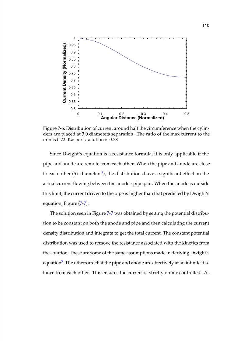
7/18/2019 Riemer PhD 2000


110

0.5

0.55

0.6

0.65

0.7

0.75

0.8

0.85

0.9

0.95

1

0 0.1 0.2 0.3 0.4 0.5

Angular Distance (Normalized)

Figure 7-6: Distribution of current around half the circumference when the cylin-ders are placed at 3.0 diameters separation. The ratio of the max current to themin is 0.72. Kasper’s solution is 0.78

Since Dwight’s equation is a resistance formula, it is only applicable if the

pipe and anode are remote from each other. When the pipe and anode are close

to each other (5+ diameters8), the distributions have a significant effect on the

actual current flowing between the anode - pipe pair. When the anode is outside

this limit, the current driven to the pipe is higher than that predicted by Dwight’s

equation, Figure (7-7).

The solution seen in Figure 7-7 was obtained by setting the potential distribu-

tion to be constant on both the anode and pipe and then calculating the current

density distribution and integrate to get the total current. The constant potential

distribution was used to remove the resistance associated with the kinetics from

the solution. These are some of the same assumptions made in deriving Dwight’s

equation3. The others are that the pipe and anode are effectively at an infinite dis-

tance from each other. This ensures the current is strictly ohmic controlled. As

7/18/2019 Riemer PhD 2000


111

0.01

0.1

1 10 100 1000 10000

Separation (pipe diameters)

T o t a l C u r r e n t ( A m

p s )

0

10

20

30

40

50

60

70

80

9058 ft Pipe/Anode

Dwight’s Equation

Error

Figure 7-7: Error in Dwight’s equation as a function of the separation of two cylin-ders. Solution given by the 3 dimensional model approaches Dwight’s solutionat large separation. The difference between Dwight’s solution and the model isdue to end effects.

7/18/2019 Riemer PhD 2000


112

can be seen in Figure 7-7, the model approaches Dwight’s solution as the pipes

are moved far from each other.

7/18/2019 Riemer PhD 2000


CHAPTER 8SOLUTION VISUALIZATION AND INTERFACE DESIGN

Figure 8-1: A screen shot and movie (click on image above) that shows some of the interactive graphics techniques needed for three dimensional geometry.

8.1 Interface Design

The interface to the model has been designed as a Microsoft Windows ap-

plication following guidelines given in “Programming the Windows 95 User In-

terface ”100 and “The Windows Interface Guidelines for Software Design”. 101

The guidelines describe how the user should interact with the data using the

mouse and keyboard. However, these two books do not provide information in

113

7/18/2019 Riemer PhD 2000


114

Figure 8-2: A screen shot of the basic window used for the interface to the model.

The window contains elements familiar to anyone who uses Microsoft Win-dows.

interaction with 3-dimensional data. For this, other sources are needed and are

described in section 8.4.

The interface starts with some common elements that most programs use and

with which most users would be familiar. First there is the main window as

shown in Figure 8-2. The window contains both a standard and application spe-

cific tool bar, a menu, and at the bottom, a status bar. The standard toolbar sup-

ports common functions such as opening and saving models. The top title bar

has the standard button to control the size of the window. The main part of the

window is where the models and their interface elements will be displayed.

A model is displayed in the main window when either a new one is created,

or one is opened. The model windows is divided into two parts (see Figure 8-3).

The left part has dual purpose. The first is calculation control and feedback, the

other is for controls related the the right section. The right-hand section is for

3-dimensional display of the model data and solutions.

7/18/2019 Riemer PhD 2000


115

Figure 8-3: A screen shot of the basic window with an empty model. The windowhas two parts: the first is for control and feedback, the other is for data display in3 dimensions.

8.2 Data Visualization

A solution of a PDE is only useful if one can examine it and derive useful

conclusion from it. One of the simplest ways to examine a solution is to plot

it versus position in the domain. This works well for a 1-D problem, but what

should be done in a 2D or 3D problem? It is possible to use a 3D graph to plot the

solution of a 2D problem on the z axis for a rectangular domain, but these types of

plots are difficult to use and precise information cannot be obtained from them.

There are no 4D graphs.

A solution to the problem is to use a 3D drawing of the domain and bound-aries. The boundaries are then colored using a color scale that corresponds to the

solution. Vectors can be overlaid on the surface to indicate flux directions (see

7/18/2019 Riemer PhD 2000


116

Figure 8-1). This technique requires the ability to interact with the data since not

all of the data can be seen simultaneously.

8.3 2D Solution Visualization

Two dimensional problems are straight forward when solutions are obtained

by the boundary element method. Since the techniques solves for the unknown

essential or natural boundary conditions, a plot of the solutions along the bound-

ary can be made.

The most meaningful plots of the solutions are either one along the length

(axial) of the pipe at a particular angle, or a plot along the circumference at some

point along the length. Extracting the necessary data involves interpolating be-

tween the nodes where the solution is known.

The first case, which is shown in Figure 8-4, is relatively simple. Here, one

simply determines the desired angular position to display and then interpolate

between the nodes where the solution is known using the shape functions of the

elements which define the variation between the nodes.

The second case is significantly more complicated. Again, one should extract

the data for the plot such that the angle from the the top of the pipe does not

change as one moves along the length extracting the data. However, as seen in

Figure 8-5, the mesh may not be regular along the surface of the pipe. Also, the

density of nodes changes in the region of the holidays, meaning simple book-

keeping that can be used to make a plot from the data in Figure 8-4 cannot be

done.

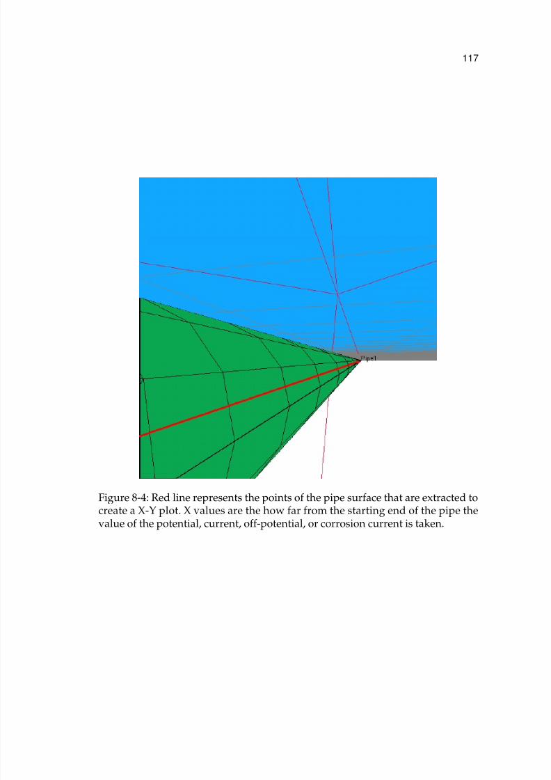
7/18/2019 Riemer PhD 2000


117

Figure 8-4: Red line represents the points of the pipe surface that are extracted tocreate a X-Y plot. X values are the how far from the starting end of the pipe thevalue of the potential, current, off-potential, or corrosion current is taken.

7/18/2019 Riemer PhD 2000


118

Figure 8-5: The red line represents the points of the pipe surface that are extractedto create a X-Y plot. X values are the how far from the starting end of the pipe thevalue of the potential, current, off-potential, or corrosion current is taken.

7/18/2019 Riemer PhD 2000


119

If rectangular holidays are used, a techniques can be devised to extract the

plot data with several extra bookkeeping structures that must be created at the

time the mesh is generated. When rectangular holidays are used, the mesh isgenerated using successive circles of nodes. If the center point, and angle of each

circle of nodes is saved along with the number of nodes that make up each circle,

then once the angular position on the pipe where the plot data is to extracted

is calculated, the plot data can be extracted one node circle at a time. At each

node circle, a calculation must be done to find the element the plot line passes

through and then the homogeneous coordinates for that point. The homogeneouscoordinates can then be used with the same element to get the desired solution

value - potential or current density.

8.4 3D Visualization

For a 3D model it is necessary to be able to visually examine the mesh for

correctness. The best available method to accomplish this is OpenGL. OpenGL

is a set of libraries distributed by Silicon Graphics in the form of an Application

Programming Interface(API) that allow an object to be drawn with correct depth

and perspective.102 If the video card is fast enough, it also can be made to be

interactive. This means that a user of the model can use a mouse to change the

viewing angle and distance from the object of interest in a true interactive fashion.

8.4.1 Using OpenGL

The code has been written using interactive techniques described by Hall and

Forsyth in their book “Interactive 3D Graphics in Windows”.103 The techniques

7/18/2019 Riemer PhD 2000


120

describe how to take the viewer into account when designing the interface. For

instance, using the mouse to control how objects move within the display is crit-

ical. The mouse is only capable of a 2-dimensional motion, but the objects mustmove in three-space in a natural intuitive way. The solution is to have several

modes of movement: zoom in/out, rotate, translate, and as a new technique in

this software, depth control. By selecting the mode of motion, movement of the

object is then restricted to that mode.

Hall and Forsyth also supplied a toolkit to learn the techniques.104 The code in

the toolkit was not used for the development of this software. Only the OpenGLAPI (application programing interface) was used.105, 106 This meant that the code

would be portable across platforms that support the OpenGL API. However,

code for other parts of the graphical user interface are not portable. Therefore

the code was separated into two distinct sections: portable code which contains

the geometry engine and most of the OpenGL drawing primitives, and non-

portable code which contains the interface elements such as windows, menus,

dialog boxes etc.

OpenGL can draw only primitive objects made up of planar triangles, poly-

gons (subdivided into planar triangles), lines and points. The boundary element

method and finite element method also uses polygons to represent the geome-

try so OpenGL is ideally suited to the task. Additionally, OpenGL can shade the

polygons, lines, and points using garuad shading based on colors specified at

the vertices of the primitive. Garaud shading is a determining the color at any

point in a triangle by linear interpolation of the colors at the vertices using the

luminescence, or RGB color model.

7/18/2019 Riemer PhD 2000


121

Figure 8-6: Shaded mesh of boundary element calculation grid. OpenGL allowsinstant visual inspection of the mesh for correctness.

Drawing the objects as they are created (meshed) provides the user with an

excellent method for feedback on its correctness. Then, if an object has been

misplaced, the user knows immediately and can fix the problem before time is

wasted with a calculation.

OpenGL uses linear interpolation schemes and is only fast when linear poly-

gons are used. This means that the polygon lies in a single plane in cartesian

coordinates. To alleviate this problem somewhat, the grid used for the calcula-

tion can be divided up into smaller sub-units over which the linear interpolation

can be applied. For instance, a nine-node Lagrangian element can be divided into

four four-node polygons each of which has a linear interpolation done, and are

then assembled piece-wise back into the surface.

7/18/2019 Riemer PhD 2000


122

Figure 8-7: Same view as figure 8-6 on page 121, with four times the number of elements. This has been done to better approximate the quadratic nature of thereal elements using linear interpolation for the graphics elements.

Figure 8-6 shows a view of a pipe with each quadratic Lagrange element di-

vided up into four linear four-sided polygons. This method does not provide a

true estimate of the paraboloid that describes the curvature of each element.

A better way to visualize the true variation of each element in both geometry

and values of potential and current when restricted to piece-wise linear 2D sur-

faces is to break each real element into 16 linear surfaces. Such a subdivision is

shown in Figure 8-7. Here, one can see how well a small number of quadratic

elements can approximate curved surfaces.

7/18/2019 Riemer PhD 2000


123

8.4.2 Coding OpenGL for BEM and FEM Meshes

Most of the code for the program was written as a set of C++ classes. Follow-

ing the philosophy of C++, objects should be self contained black boxes when

complete. One of the necessary functions of all geometry objects is that they can

draw themselves into the OpenGL rendering engine. Therefore the base class

of all geometry classes contains a method Render(PARAMS *pParams) which

handles drawing tasks for all derived geometry objects. The single argument

contains some necessary information such as whether to use shaded polygons or

a wireframe and if shaded, which color set to use (potential, current, corrosion

current, etc.) This bases class maintains the list of nodes and elements used to

describe the geometry.

An example Render routine that draws a wire frame is given in Appendix B.

Before Render is called, the OpenGL engine is told how all polygons sent to

it should be rendered. For wire frame it would be:

glPolygonMode(GL_FRONT_AND_BACK,GL_LINE);

Other commands can tell the engine to fill the polygons with a color, or to inter-

polate the color at every point within the polygon by the colors at the vertices.

Setting up the OpenGL engine is platform dependent and one should refer to

the appropriate literature for their platform. Because of this, the setup for this

software is contained in the interface code. Appendix B has the setup necessaryfor the Microsoft platform.

7/18/2019 Riemer PhD 2000


124

8.5 Visual Feedback

Feedback of the results of a calculation to the user can be done in a number

of ways. The first is to use an object that the field engineer will be familiar with,

a Cu/CuSO4 reference electrode. The electrode can then be moved over the sur-

face of a pipe to get a reading of the desired quantity. Unlike a real reference

electrode, a software version can output more than just a potential. The reference

electrode used in model provides on-potential, off-potential, net current, and cor-

rosion current.

7/18/2019 Riemer PhD 2000


CHAPTER 9COMPUTATIONAL PERFORMANCE

Computer performance for the boundary element method is a very active area

of research.107 Since most of the computational time is spent evaluating the inte-

grals in equation (3-9) on page 32, it is the best place to look for performance

improvements. One of the best ways to improve the speed after algorithms

have been optimized is to use a parallel computer architecture. Since it is much

cheaper to hook several single cpu machines together with a network than to buy

a multi-CPU machine and that such arrangements are readily available in most

university and industrial settings, this approach will be used.

9.1 Parrallel Computing Methods

There are several ways to break down the Boundary Element Method into

tasks that can be executed in parallel.

The smallest tasks that can be executed in parallel are the calculation of the

individual Gauss-Kronrod points. In this method, each CPU available evaluates

one point until all the points have been calculated. For this method to be effi-

cient, an extremely high speed bus, cache and memory must be present or all of

the CPUs may have to wait for one CPU to put its result into memory to allow

calculation of the final value of the integral can be calculated. This method is very

efficient on vector type computers(Cray C-90, Y-MP) and on shared memory pro-

cessor arrays (SGI Origin 2000, Intel Paragon). Each processor caches its gauss

125

7/18/2019 Riemer PhD 2000


126

point data and instructions and simply receives the physical element where the

point will be evaluated. This allows for efficient use of CPU power but requires

very precise timing. It fairs very poorly in distributed environments.The next level up in the size of a parallel task is for each CPU to perform an

entire single integration. In this scenario, each cpu receives a set of data necessary

to complete a single integral. This integral forms a single entry in one of the

matrices in equation (4-2). This method also works well in small processor arrays

and for small distributed memory computers. The downside of this method is

that the ratio of time spent communicating between processors to the time spentin calculation higher.

A further enhancement to the previous method is to calculate all the integrals

associated with a point-element pair. In the case of a 3D problem using linear

triangles, there would be 6 integrals to be done using a single set of data. If

quadratic Lagrangian elements are used the number jumps to 18 integrals. At

this level, the ratio of communication to calculation has been minimized. It is

now a matter of determining when the communication takes place. One can as-

sign a CPU a block of point-element pairs and send all the necessary data at the

beginning of the calculation. Another choice would be to send the point-element

pairs immediately after each set of integrals have been completed and results

returned.

9.2 Processor Arrays

These types of computers are made up of a single large block of physical mem-

ory with a large number of processors having access to the memory. The SGI

7/18/2019 Riemer PhD 2000


127

Origin 2000 and Intel Paragon are examples of these types of computers. They

have the potential of being the fastest of all types of supercomputers. Generally,

the use the first of the parallel techniques as described above.

9.3 Distributed Computation Methods

This class of computer is actually many separate computers linked by a stan-

dard networking system. Instead of being able to directly address another proces-

sor in the computer, a software layer is required to perform the communication.

Another problem, is that the memory is also distributed, so any data needed by

the a processor must also be sent along with the calculation commands. This

means that the level at which the parallelism is made must be at a coarser level

than what is typically done with a processor array type computer.

The point at which the parallelism is applied depends greatly on the overhead

of communicating the necessary data and calculation commands to the comput-

ers making up the parallel machine. It is important that the overhead of commu-

nicating is less than the time required to perform the calculation or the gain of

having multiple CPUs is lost.108 Many people have solved this problem by sim-

ply assigning each machine a large block of the matrices that appear in equation

(4-2). The method assumes that all the CPUs have the same performance capabil-

ities and that no other processes are running. It also does not allow for any error.

If for some reason one of the computers crashes, shuts down or loses contact with

the rest of the computers, the entire calculation must be restarted.

There are several codes available to handle the data and command communi-

cation between networks of computers linked into a single distributed computer.

7/18/2019 Riemer PhD 2000


128

These include Parallel Virtual Machine (PVM), and Message Passing Interface

(MPI). For the work done here a new approach has been taken. The new method

makes use of a faster and lower level interface for inter-computer communica-tion called Remote Procedure Call (RPC). RPC allows a computer program to call

a subroutine that actually runs on a separate computer. Section C.3 of Appendix

C contains details for writing RPC code to separate functions onto several com-

puters.

9.4 Communication Between Computers

Computers forming the parallel machine must have a method to communi-

cate data to each other. The communication can be greatly simplified if takes a

master/slave approach to the problem. This approach can also be referred to as

a star configuration with the master computer at the center of the star.

In a star configuration, the master computer takes the input from the user and

constructs the mesh for the problem. Boundary conditions are supplied by the

user. The master computer then splits up the calculation according to the parallel

method being used and sends tasks out to each computer in the star. When the

outer point computers complete the assigned task, they return the results to the

central computer. The central computer compiles the various result to form the

complete solution. Code for the communication on both the client and server

side of the RPC is contained in section C.3 of Appendix C.

A plot of the performance of a distributed network of computers using RPC

as the low-level communications layer is shown if Figure 9-1.

7/18/2019 Riemer PhD 2000


129

0

400

800

1200

0 400 800 1200

Expected Value (MFLOPS)

A c t u a l S c a l i n g ( M F L

O P S )

Figure 9-1: Plot of performance vs expected performance for a distributed com-puter.

Table 9.1: Comparison of location of integration source code.

Calculation module used Time to complete Calculation

Compiled into main program 00:02:47Small separate program 00:01:21

9.5 Improving Performance by Separating Calculation Code

A very interesting by product of separating the calculation of the integrals into

a separately compiled program that can run on many computers simultaneously,

is that on a stand alone setup, the performance can be substantially improved.

This is done by installing the remote module on the stand-alone machine and

telling the main program to use its own remote module. A simple test gave the

results in Table 9.1. The reason for the difference is fairly simple. The amount

of data needed by the small integration module is very small and can usually

7/18/2019 Riemer PhD 2000


130

fit within the CPU cache. This is referred to as good locality of data. The main

program also has to keep track of where in the main matrices the data returned

by the integration is to be placed, and update information to the user.

9.6 Benchmarks and Scaling

In a heterogeneous computing environment a method is needed to gauge the

efficiency of adding more machines to the effort. A consistent method must be

used to determine the efficiency of process and the computational power applied

to solve the problem.

To evaluate the system of computers used to perform the boundary element

calculations, a benchmark is performed using one computer to determine the

number of FLOPS needed to complete an example calculation. Then each com-

puter was timed using a random selection of integrals to establish what its maxi-

mum stand-alone performance would be. The results have been normalized and

are shown in Table 9.2. These results have been checked by using them to pre-

dict the time required to solve a real problem and have been found to be accurate

to within 5%. By normalizing the result with respect to the master computer,

any differences that may have occurred because of the selection of integrals is

removed. Since the total FLOPS used to complete the calculation are known, the

real throughput of the parallel computer can be estimated.

Evaluation of the heterogeneous distributed computer was done using an ac-

tual model of a coated pipeline with coating holidays and a 5 anode ground bed.

The total number of floating point operations needed to evaluate all of the inte-

grals in equation 3-9 amounted to 143,500 mega-FLOPS. A machine with a sus-

7/18/2019 Riemer PhD 2000


131

Table 9.2: Normalized benchmark result data for many types of computers.

Machine Processor OS and RAM Result

1 Pentium II 300Mhz NT 4.0, 384MB 1.02 Alpha 21164, 300Mhz NT Server 4.0, 128MB 0.9763 Pentium II 300Mhz NT 4.0, 128MB 0.9234 Pentium, 133Mhz NT 4.0, 32MB 0.298

5 Pentium 84Mhz NT 4.0, 32MB 0.0886 Pentium 200Mhz NT 4.0, 32MB 0.4397 Pentium 225Mhz NT 4.0, 32MB 0.4948 Pentium 200Mhz Windows 98, 32MB 0.4119 Pentium 133Mhz NT 4.0, 32MB 0.296

10 Pentium 100Mhz NT 4.0, 32MB 0.22511 Pentium 100Mhz NT 4.0, 32MB 0.29712 Dual Pentium 200 NT 4.0, 128MB 0.80613 Pentium 133Mhz Window 95, 48MB 0.29214 AMD K6 300Mhz NT 4.0, 64MB 0.41915 Pentium 83Mhz NT 4.0, 40MB 0.100

16 i486 66hz NT 4.0, 32MB 0.03017 Pentium 120Mhz NT 4.0, 48MB 0.29618 Pentium 133Mhz NT 4.0, 64MB 0.29619 Pentium Pro 200 NT 4.0, 128MB 0.55320 Pentium 200Mhz NT 4.0 Server, 64MB 0.45021 Pentium II 233Mhz NT 4.0, 64MB 0.74722 Pentium II 233Mhz NT 4.0, 128MB 0.77323 Pentium 200Mhz NT 4.0, 32MB 0.40724 Pentium 200Mhz NT 4.0, 64MB 0.44225 Pentium II 233Mhz NT 4.0, 64MB 0.762

7/18/2019 Riemer PhD 2000


132

tained through-put of 100 mega-FLOPS/sec would need ∼25 minutes to com-

plete the calculation.

A timing mechanism was built into the software to check the wall-clock time before and after the calculation was done. Using the time and the number of float-

ing point operations needed, an average through-put for the distributed com-

puter could be found.

The procedure used to build a performance scaling line was to run the model

first on the master only to get the first point in the line. Then machines were

added to the distributed computer, 1 at a time, with the model being run onceas each computer was added. To eliminate any effect that the order of adding

computers may have on the shape of the line, several runs were made of adding

all of the available computers using a different random order of machine addition

for each run. An example run is shown in Table 9.3.

Often, with distributed machines, the actual node in the machine may be used

for some job by another user. This effect can be seen in the center section of rows

in Table 9.3. Those machines that are under heavy use by other users contribute

very little to the distributed computer. On the other hand, if there is very little

external activity, the performance scales very well. An abbreviated table of data

is shown in Table 9.4. Figure 9-1 shows the pooling of several runs of the type

shown in table 9.3. In this case, linear scaling through all of the machines is

seen up to about 800 mega-FLOPS which corresponds to 12.5 times the speed

of the master computer. Scaling is still good through the tested range of 1100

mega-FLOPS or 17.2 times the master computer speed.

7/18/2019 Riemer PhD 2000


133

Table 9.3: An example run of the scaling of a heterogeneous distributed computer.Computers are added one by one and the model is timed with each additionalcomputer. This particular run was done when many of the workstations werealso being utilized by other users.

Order Expected Pwr Time Actual Pwr Expected MFLPS Actual MFLPS

1 1.00 1.00 63.99 63.9922 2.51 859.2 2.61 160.5 167.07 3.77 569.0 3.94 241.2 252.2

11 4.10 518.2 4.33 262.4 276.910 4.51 479.0 4.68 288.7 299.624 5.45 420.0 5.34 348.4 341.720 5.81 394.0 5.69 371.6 364.226 6.43 356.0 6.30 411.8 403.118 6.55 350.0 6.41 419.1 410.021 6.88 337.0 6.65 440.3 425.814 8.07 284.0 7.90 516.4 505.38 8.56 268.0 8.37 547.7 535.4

17 9.04 255.1 8.79 578.3 562.43 10.4 226.2 9.92 662.4 634.5

19 10.9 225.0 9.97 700.1 637.613 11.3 220.0 10.2 721.4 652.24 12.1 225.2 9.96 772.0 637.2

27 12.7 218.0 10.3 812.5 658.328 12.9 229.2 9.79 822.8 626.216 13.0 209.2 10.7 832.5 685.915 13.5 193.0 11.6 864.3 743.523 14.5 176.0 12.7 924.6 815.325 15.0 183.0 12.3 959.1 784.19 15.5 177.0 12.7 994.5 810.72 16.5 170.0 13.2 1058 844.0

12 16.8 165.1 13.6 1075 869.0

7/18/2019 Riemer PhD 2000


134

Table 9.4: An second example run of the scaling of a heterogeneous distributedcomputer. This run shows better scaling because the load from other users wasless.

Order Expected Pwr Time Actual Pwr Expected MFLPS Actual MFLPS

1 1.00 1.00 63.99 63.9922 2.51 839.3 2.67 160.5 171.03 3.82 586.0 3.83 244.6 244.9...

... ...

... ...

...19 9.56 251.0 8.93 612.0 571.7...

... ...

... ...

...4 16.8 140.1 16.0 1075 1025

It is apparent that this method will scale up to the greatest amount of free

CPU time available on all of the machines within a distributed computer. This

will happen irregardless of the load placed by other users.

9.7 Hard Drive Performance

Loading and saving data from persistent storage can be a source of slow per-

formance. If data is not written or read as a continuous stream, performance can

degrade by over a factor of 100. It is also advantageous to have only one of the

matrices ( H or G) in RAM at any time and to have both matrices only in persis-

tent storage when forming the A matrix. This can increase the size of the solvable

problem by a factor of √

2.

Since it will be necessary to swap columns between the H and G matrices, it

is best to store these matrices in the FORTRAN style column major order. This is

opposed to C/C++, where the natural form is row major. Some experiments were

done using a small set of matrices and a large set. The first experiment involved

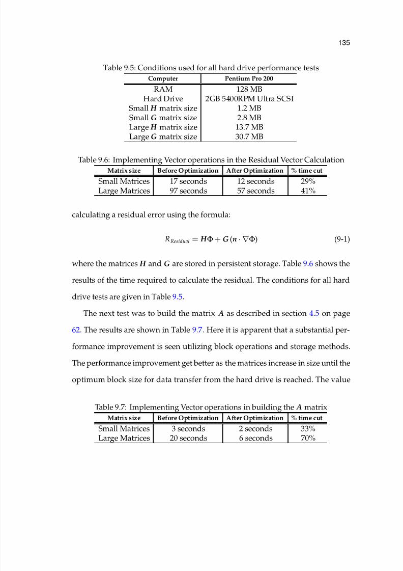
7/18/2019 Riemer PhD 2000


135

Table 9.5: Conditions used for all hard drive performance tests

Computer Pentium Pro 200

RAM 128 MB

Hard Drive 2GB 5400RPM Ultra SCSISmall H matrix size 1.2 MBSmall G matrix size 2.8 MBLarge H matrix size 13.7 MBLarge G matrix size 30.7 MB

Table 9.6: Implementing Vector operations in the Residual Vector Calculation

Matrix size Before Optimization After Optimization % time cut

Small Matrices 17 seconds 12 seconds 29%Large Matrices 97 seconds 57 seconds 41%

calculating a residual error using the formula:

RResidual = H Φ+G (n · ∇Φ) (9-1)

where the matrices H and G are stored in persistent storage. Table 9.6 shows the

results of the time required to calculate the residual. The conditions for all hard

drive tests are given in Table 9.5.The next test was to build the matrix A as described in section 4.5 on page

62. The results are shown in Table 9.7. Here it is apparent that a substantial per-

formance improvement is seen utilizing block operations and storage methods.

The performance improvement get better as the matrices increase in size until the

optimum block size for data transfer from the hard drive is reached. The value

Table 9.7: Implementing Vector operations in building the A matrix

Matrix size Before Optimization After Optimization % time cut

Small Matrices 3 seconds 2 seconds 33%Large Matrices 20 seconds 6 seconds 70%

7/18/2019 Riemer PhD 2000


136

varies from drive to drive but is usually between 16K and 64K. 64K corresponds

to 8192 double precision floating point numbers.

9.8 High Performance Libraries

CPU manufacturers often make special high performance libraries available

for their processors. Intel has built a set of well tuned libraries as made them

freely usable in compiled form.98 These libraries have the added benefit in that

they can utilize more than one processor on the machine where the code is run.

Intel’s data shows linear scaling of CPU efficiency on up to four processors. The

code has been tested for this work on single and dual processor machines and

linear scaling is seen.

Intel also supplies optimized math functions such as ln, exp, sin and cos. A

factor of 2 improvement over the stdlibc routines that accompany all compilers

can be seen.

7/18/2019 Riemer PhD 2000


CHAPTER 10HOLIDAY EFFECTS ON SINGLE PIPES AND PIPELINE NETWORKS

The goal of this research was to be able to predict the effects seen in current

and potential distributions in pipeline networks. One contributing item was coat-

ing holidays. Coating holidays are a small sections of the pipe where the coating

has somehow been removed from the pipe and bare steel is exposed to the soil

environment (see Figure 10-1).

Figure 10-1: Pipe that exhibits many coating holidays. Pipe was coated in the late60’s and dug up in 1996.2

The early work by Kennelly et al. 109 and Orazem et al. 110 on modeling the

influence of coating holidays employed the Finite Element Method. While their

results showed that the majority of current from the CP system went to the hol-

iday, there was a significant error in the closure of current (3% to > 12%) when

modeling holidays.109 Thus, their work demonstrated the weakness of using the

classical finite element method where the flux is calculated from potential gradi-

137

7/18/2019 Riemer PhD 2000


138

ents. In subsequent work, a boundary-element approach was used to model the

role of coating holidays.33, 111, 112 The geometry considered was a single pipeline

protected by sacrificial ribbon anodes such as those used for the Trans-Alaskapipeline. As constant triangular elements were used to discretize the surfaces, a

large number of triangles were required to model properly the discontinuity of

the current near the coating-holiday edge. Their work supported the conclusion

that it is much more difficult to drive current to a holiday than to a uniformly poor

coating. The results of the model for a pipe protected by ribbon anodes showed

that the variation of potential around the pipe at a holiday can be as large as 550-650mV. This value is the difference between the most cathodic potential on the

coated pipe and the most anodic potential at the holiday. Numerical difficulties

limited the application of the model to short sections of pipe (<40 ft.).

10.1 Single Pipes

The first effect of holidays to investigate is to see how the current and po-

tential distributions are effected by the presence of a holiday on a single pipe.

Orazem et al. 110 first demonstrated the effects. Figure 10-2 shows a large holiday

in an 18in-diameter pipe. The pipe is protected by a remote impressed-current CP

system operating at -10 volts from the connection to the pipe. At the edge of the

coating next to the holiday, the off-potential reading dips by 30 mV to -850 mV

Cu/CuSO4 which is marginally protected. The holiday has the greatest potential

at the center, -863 mV Cu/CuSO4. It might be expected that the coated region

close to the edge of the holiday is in the worst shape. However, the corrosion rate

is what is most important. Examining the corrosion rate at the center of the holi-

7/18/2019 Riemer PhD 2000


139

Figure 10-2: Off-potential distribution for a large holiday in a good quality coat-ing. The edge of the coating next to the holiday does not meet the -850 mV cri-terion while the holiday does. Even so, the corrosion rate at the holiday is muchhigher than at any of the coated sections.

day reveals that it is corroding at a rate that is 3 orders of magnitude higher than

that under the coating. The reason for the low rate under the coating is that the

coating causes the rate of oxygen transport to be decreased and it adheres to the

steel substrate. Recent experiments by Corfias et al. have begun to characterize

the transport of electrolytes through coating, and how water uptake affects pore

size, adherence properties and transport.27 They have shown that electrochemical

reactions (corrosion, oxygen reduction, etc.) are taking place at the steel surface

and the rates are reduced by the coating.

If the CP system output is increased, the phenomenon seen in Figure 10-2 is

still observed with larger variations in the off-potential of the coating. A plot of

the angular potential and current distributions around the pipe at the holiday

is given in Figure 10-3. In this case the off-potential of the coating exhibits a 50

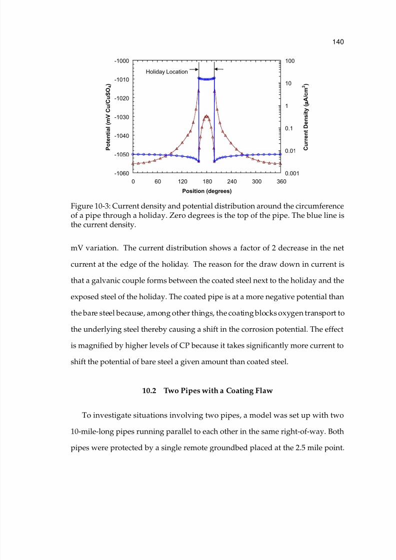
7/18/2019 Riemer PhD 2000


140

-1060

-1050

-1040

-1030

-1020

-1010

-1000

0 60 120 180 240 300 360

Position (degrees)

P o t e n t i a l ( m V C u / C u

S O 4 )

0.001

0.01

0.1

1

10

100

C u r r e n t D e n s i t y ( µ µ µ µ A / c m

2 )

Holiday Location

Figure 10-3: Current density and potential distribution around the circumferenceof a pipe through a holiday. Zero degrees is the top of the pipe. The blue line isthe current density.

mV variation. The current distribution shows a factor of 2 decrease in the net

current at the edge of the holiday. The reason for the draw down in current is

that a galvanic couple forms between the coated steel next to the holiday and the

exposed steel of the holiday. The coated pipe is at a more negative potential than

the bare steel because, among other things, the coating blocks oxygen transport to

the underlying steel thereby causing a shift in the corrosion potential. The effect

is magnified by higher levels of CP because it takes significantly more current to

shift the potential of bare steel a given amount than coated steel.

10.2 Two Pipes with a Coating Flaw

To investigate situations involving two pipes, a model was set up with two

10-mile-long pipes running parallel to each other in the same right-of-way. Both

pipes were protected by a single remote groundbed placed at the 2.5 mile point.

7/18/2019 Riemer PhD 2000


141

-850

-800

-750

-700

-650

-600

-550

0 60 120 180 240 300 360

Position (degrees)

O f f - P o t e n t i a l ( m V C u / C u S O 4 )

0.00001

0.0001

0.001

0.01

0.1

1

10

C u r r e n t D e n s i t y ( µ µ µ µ A

/ c m

2 )

Holiday Location

Figure 10-4: Current density and potential distribution around the circumferenceof a pipe through an under-protected holiday. Zero degrees is the top of the pipe.The blue line is the current density.

The coating of the flawed pipe was assumed to be aged. The adjacent pipe was

assumed to have a high-quality coating.

Figure 10-4 shows the potential and current density distribution around the

circumference of the pipe at the point of the holiday. The holiday is under-

protected at the center and is corroding at a rate of about 0.5 mils per year. The

current density near the holiday is an order of magnitude smaller than that seen

far from the holiday.

The adjacent pipe shows some effects of the neighboring coating holiday. Fig-

ure 10-5 shows the off-potential and current density distributions for the well-

coated pipe. The effect of the holiday is apparent but it is not to the extent of

that seen for the pipe with the holiday. The effect is called shadowing. The cusp

seen at the distributions is a numerical effect due to the joint between elements

occurring exactly at the point of closest approach. The effect can be removed by

7/18/2019 Riemer PhD 2000


142

-850

-845

-840

-835

0 60 120 180 240 300 360

Position (Degrees)


0.00015

0.00016

0.00017

0.00018

0.00019

0.0002

C u r r e n t D e n s i t y ( µ µ µ µ A

/ c m

2 )

Figure 10-5: Current density and potential distribution around the circumferenceof a pipe at the spot closest to the under-protected holiday on the neighboringpipe. Zero degrees is the top of the pipe. The blue line is the current density.

changing the number of elements used to create the mesh around the circumfer-

ence of the pipe such that the center point of an element is at the point of closest

approach.

20 feet away from the holiday, the potential distribution on the well-coated

pipe is much closer to uniform and all points around the circumference are pro-

tected. Even though the section of pipe closest to the holiday has fallen below the

-850 mV criteria, the rate of corrosion under the coating is negligible.

10.3 Pipes Exhibiting Stray Current

A technique to allow the possibility of stray current between different CP sys-

tems was developed Section 4.3. A pipeline network was setup as shown in Fig-

ure 10-6. For this system, two pipes were placed adjacent to each other with one

7/18/2019 Riemer PhD 2000


143

Figure 10-6: Distant view of a under-protected holiday. Lower right portion of pipe with holiday is also exhibiting stray current.

pipe leaving the right-of-way at a 45 degree angle 1 mile from the starting point

of the model. The diverging pipe was given two different coatings of the form of

equations (1-24) an d(1-25). One was for the section that ran parallel to the second

pipe with parameters to emulate an “aged” coating. The other section consisting

of the part diverging away from the second pipe was given a new coating similar

to the original. The second pipe was considered to have a new coating except

for a holiday at the bend in the pipe. The two pipes have separate CP systems

consisting of distributed groundbeds that are relatively close to each other. This

scenario can be thought of as an old oil pipeline and a new gas pipeline sharing a

portion of a single right-of-way. The model was used to examine the point where

the two pipelines merged into a single right-of-way.

A small portion of the pipes being modeled is shown in Figure 10-7. The shad-

ing represents the calculated potential distribution around the pipe. The stray

current associated with the two CP systems caused a portion of well-coated pipe

7/18/2019 Riemer PhD 2000


144

Figure 10-7: Closeup of an under-protected holiday.

to serve as an anode, delivering current to the poorly-coated pipe. This effect is

seen more clearly in Figure 10-8 where the current distribution around the well-

coated pipe is presented as a function of angular position. The corresponding

potential distribution is given in Figure 10-9 for a section of the pipe exhibiting

stray current effects and for a section of the pipe farthest from the section of the

pipe that exhibits stray current effects. In the region where stray current effects

are evident, the entire pipe falls below the -850 mV Cu/CuSO4 protection cri-

terion. The point closest to the neighboring poorly-coated pipe is anodic, and

the section opposite the neighboring pipe is at only slightly cathodic potentials.

These results can be compared to the current distribution given in Figure 10-8

where the positive current is anodic.

Even in the section of the pipe that was not driven to anodic currents by the

interference between CP systems, the pipe is not adequately protected in the re-

gion that is closest to the neighboring pipe. For this system, rectifier settings

7/18/2019 Riemer PhD 2000


145

Position (degrees)0 90 180 270 360

C u r r e n t D e n s i t y ( µ A / c m

2 )

-1

0

1

2

Figure 10-8: Current Density around pipe in area exhibiting stray current in Fig-ure 10-7. Positive current densities are anodic.

Position (degrees)

0 90 180 270 360

P o t e n t i a l ( m V C u / C u S O 4

)

-1000

-900

-800

-700

-600

-500

Point farthest fromneighboring pipe Point closest to

neighboring pipe-850 mV Cu/CuSO

4

Figure 10-9: Potential distribution around pipe at center of section exhibitingstray current and at end of section where all parts of the circumference of thepipe are cathodic.

7/18/2019 Riemer PhD 2000


146

Figure 10-10: Distant view of soil surface on-potentials over an under-protectedholiday.

could be found that would cause the entire system to meet or exceed the -850

mV Cu/CuSO4 criterion, but, in doing so, a significant portion of the pipeline

was over-protected. Satisfactory protection for this case was achieved only when

the pipes were bonded such that stray current effects were eliminated. Again, the

smooth distributions presented in Figure 10-8 and Figure 10-9 reflect the accuracy

of the meshing and the adaptive integration schemes used in these calculations.

10.4 Soil Surface On-Potentials

Soil surface on-potential distributions were calculated for the pipes exhibiting

stray current described in section 10.3. If there is going to be much to see in an on-

potential survey of the pipe, the results of section 10.3 should show it. Figures 10-

10 and 10-11 show the on-potential distributions. Figure 10-11 has been split so it

is apparent where the pipes are located with respect to the soil surface calculation.

On-potential surveys near the anodes tend to only show the anodes. This is made

7/18/2019 Riemer PhD 2000


147

Figure 10-11: Distant view of soil surface on-potentials with a portion of the soilsurface removed to see the pipe. The soil surface on-potential only indicates thepresence of the anodes. The holiday is not seen.

apparent in the calculations. The interference of the anodes masks the behaviour

of the pipes and even the stray current situation. The only indications of the pipe

are in the upper left corner where a portion of the well-coated/well-protected

section of pipe is seen.

10.5 Adjacent Holidays

An issue brought up in discussions with pipeline operators was whether an

under-protected large coating holiday next to a small holiday would adversely ef-

fect the small holiday. To test the idea, a model was setup with two holidays very

close to each other (see Figure 10-12). The large holiday exposed 17.7 cm2 bare

steel. The small holiday exposed 12.6 mm2 of steel. The holidays were placed

with 2.91 cm space between them. This was the closest that two holidays could

be placed using the mesh generator. Both holidays were assumed to have the

7/18/2019 Riemer PhD 2000


148

(a) Dimensions (b) Mesh

Figure 10-12: Setup for calculation of a pinhole holiday next to a large holiday: a)the dimensions of the holidays and b) the automatically generated mesh for theholidays.

same polarization curve (equation (1-23)) and parameters. The CP system was

set such that the large holiday was under-protected. Figure 10-13 shows the off-

potential distribution of the two holidays. From the color scale, it is apparent that

all but the edges of the large holiday are under-protected. The small holiday re-

mains well protected even though it is close to a holiday that is under-protected.

Therefore, the situations that should concern pipeline operators are large coat-

ing holidays. These are the most difficult to protect so monitoring systems need

to indicate when a problem will occur on a large holiday versus a small one.

Chapter 11 discusses one monitoring technique and how the size of holidays af-

fect the technique.

7/18/2019 Riemer PhD 2000


149

Figure 10-13: Off-potential distribution of a pinhole holiday next to a large holi-day. The large holiday is under-protected by standard criteria while the pinholeis well protected.

7/18/2019 Riemer PhD 2000


CHAPTER 11COUPONS

Coupons are a small piece of pipeline grade steel placed in the same soil envi-

ronment as the pipeline. The coupon is connected to the CP system through a test

station so the polarization level of the coupon can be monitored without affect-

ing the CP provided to the pipe. It is thought that a coupon represents a holiday

of similar size. Mathematical models were used to explore the conditions un-

der which a coupon provides a conservative assessment of the level of cathodic

protection provided to holidays on coating buried structures. The most conserva-

tive assessment of cathodic protection was obtained when the area of the coupon

was larger than the area of the largest expected holiday. The performance of the

coupon as a monitor of cathodic protection was found to be strongly influenced

by the availability of oxygen in the soil.

11.1 Introduction

The true off-potential of holidays on cathodically protected buried pipelines

can be difficult to ascertain. Normally, all that can be obtained is the off-potential

of the pipeline itself which is said to represent some kind of a weighted average

of the true off-potential of all the holidays. When one cannot remove all sources

of current, it is not possible to get an off-potential measurement. Such compli-

cating factors include direct bonded galvanic anodes, telluric currents, and stray

currents.

150

7/18/2019 Riemer PhD 2000


151

The pipeline off-potential may not be representative of the off-potential at a

large holiday if there are many smaller holidays also on the pipe which sum

to a similar area as the larger holiday. One solution to this problem is to use acoupon. Coupons have been proposed to be an alternative or a complement to

direct measurement of off-potentials for assessing cathodic protection of buried

structures.113, 114, 115 The coupon can be connected to the pipe or CP system through

a test station in such a way that all sources of current to the coupon may be turned

off without disrupting the current to the pipeline. It has been recommended

that a coupon be as similar as possible to a section of the actual structure be-ing protected.3, 114 However, there has been little theoretical work done to show

the relationship between a holiday of a given size on a pipeline and a coupon.

Stears et al.114 and Lawson and Thompson115 showed that the off-potentials

measured for coupons varied with location relative to the pipeline. This result

can be attributed to differences in soil environments. The mass-transfer-limited

current density for reduction of oxygen has a critical influence on the corrosion

potential, and variations due to differences in moisture content or soil composi-

tion will influence the coupon off-potential. Coupon configuration, location, and

size can also influence coupon readings. Lawson and Thompson115 observed that

small coupons tended to be polarized more than large coupons. This observation

is consistent with the calculations presented by Orazem et al.33, 109, 110, 111 Lawson

and Thompson115 also reported that in some cases, the coupon off-potential was

significantly more negative than the off-potential of the pipe, suggesting that the

exposed surface area was greater on the pipe than on the coupon. The differ-

ence between coupon and pipe off-potentials was influenced by the amount of

7/18/2019 Riemer PhD 2000


152

cathodic protection current applied, although no general trend could be identi-

fied. The difference between coupon and pipe off-potential was generally small,

but, in some cases, was on the order of 200 mV. The biggest differences were seenfor cases where the coupon reading of -780 mV indicated that a 200 mV potential

shift criterion was met but where the pipe off-potential of -580 mV suggested that

the pipe was underprotected.

Safe utilization of coupons for assessing the level of protection afforded by

a cathodic protection system requires a better understanding of the factors that

influence the coupon readings relative to pipe condition. This work takes a first-principles approach to identify the relationship between the off-potential of a

coupon and the off-potential of a holiday through the solution of the governing

differential equations. Recently published experimental work 114, 115 provides a

basis for comparison to the models. Their work indicates that there should be a

relationship between the shift in the off-potential of a coupon due to a change in

the setting of a rectifier and the change in the off-potential of a pipe with coating

holidays and that they both change in the same direction.

It should be noted that, because the calculations provide detailed results for

individual holidays, the modeling approach presented here should yield greater

insight into the relationship among coupons and holidays than can be obtained

from experiments conducted on pipelines where measured off-potentials reflect

a weighted average of the behavior of all holidays.

7/18/2019 Riemer PhD 2000


153

Table 11.1: Polarization parameters used in the model.41

Parameter Values

ilim,O2 0.1, 1.0, 3.16, 10.0 µA/cm2

EFe -526 mV(CSE)β Fe 59 mV/decadeEO2

-104 mV(CSE)β O2

59 mV/decadeEH2

-955 mV(CSE)β H2

118 mV/decade

11.2 Boundary Condition Parameters

The model is capable of assigning different individual polarization curves to

each coupon and holiday. A coupon with a new bright finish, for example, would

be characterized by a polarization curve with a large mass-transfer-limited cur-

rent density for oxygen reduction; whereas, to account for the presence of scale

deposits, a holiday on an old pipe would be characterized by a polarization curve

with a smaller mass-transfer-limited-current density for oxygen reduction. The

code can also handle many holidays on the same pipe, each sized differently and

with different polarization curves.

The polarization curve used for bare metal surfaces (coupons and holidays)

was equation (1-23). The parameter values for equation (1-23) are given in Table

(11.1).

The coating was modeled using a set of equations given in Chapter 1. The

values in Table 11.1 were used for the polarization behavior of the steel beneath

the coating and the addition parameters listed in Table 11.2 determined from ex-

perimental data.24, 111

7/18/2019 Riemer PhD 2000


154

Table 11.2: Coating parameters used in model. Note: These parameters weredetermined after water uptake of the coating.116

Parameter Values A/ Apore 1000ρ 5 × 109 Ohm-cmδ 20 mil

α block 0.99 (99% effective)

11.3 Approach

The pipeline used for the model was 6.44 km in length and had a diameter

of 457 mm. The pipe was protected by a single impressed current ground bed at

one end of the pipe section. The holiday-free sections of the pipe were assumed

to have a uniform 0.5 mm (20 mil) FBE coating. Coating holidays were assumed

to expose bare steel. The anode used for this model was an impressed-current

ground bed, sized at 76 mm OD and 15.25 m length. Its current output could

be adjusted until the desired reading of the off potential for the coupon was ob-

tained.

Two coupon designs were used for the simple cases. The first was a band

of bare steel of length 6.35 cm on a 5.08 cm diameter pipe which follows the

design described by Stears et al.114 The second was a 1.27 cm rod with an exposed

tip of 2.5 cm which follows the design described by Lawson and Thompson.115

Schematic representations of the coupons are given in Figures 11.1(a) and 11.1(b)

respectively.

Two sets of calculations were performed. One set involved a single holiday

with a single coupon. The coupon was placed 6 meters from the holiday with 1.2

m top cover over the exposed portion. For each of the coupon types, four ratios

7/18/2019 Riemer PhD 2000


155

(a) (b)

Figure 11-1: Schematic representations of the two cylindrical coupons used in thesimulations: a) large coupon114 with a surface area of ∼ 50 cm2; and b) smallercoupon115 with a surface area of 9.5 cm2.

of the holiday area to the coupon area were used. For each of these cases, four

different polarization curves were used. Finally the current output of the anode

was adjusted iteratively such that the average off-potential of the coupon was -

750, -850, or -950 mV CSE. The calculation matrix therefore included 96 different

cases.

The more complicated scenario involved the same pipe and anode, but the

pipe was assumed to have five coating holidays of different sizes. Three of the of

them were placed at the top of the pipe (0o), and the remaining two were placed at

the bottom (180o). The bottom of the pipe was assumed to rest in water-saturated

soil while the top was assumed to be in dry soil. To simulate the influence of

water level, the holidays at the bottom of the pipe were assigned a polarization

7/18/2019 Riemer PhD 2000


156

curve with a i lim,O2 that was an order of magnitude lower than that used for the

holidays at the top of the pipe.

The design of the large coupon was changed for the more complicated sce-nario. From the results of the first simulations, it was apparent that there may

be an effect associated with the geometry of the coupon. To provide a prelimi-

nary exploration of the role of coupon design, the large coupon was redesigned

to match closely the design of the small coupon, Figure 11.1(b), but with the same

surface area as the original coupon.

11.4 Results and Discussion

The difference between the measured potential of the coupon and the most

positive potential on the holiday is presented in Figure 11-2 for the large coupon.

The corresponding results for the small coupon are given in Figure 11-3.

The presentation of calculated results as the difference between the measured

potential of the coupon and the most positive potential seen on the holiday em-

phasizes the behavior of the system where the corrosion rate is the highest. The

sign on the y-axis indicates whether the holiday is at a more cathodic potential

(negative sign in front) or at a more anodic potential than the coupon. Both sets

of simulations used the same convention.

As seen in Figures 11-2 and 11-3, the coupon does not provide an exact mir-

roring of the behavior of the holidays. As reported by Lawson and Thompson,115

a change in the rectifier output results in a similar shift in the off-potential of the

coupon and the holiday. The reliability of the coupon off-potential as an indi-

cator of the holiday off-potential depends strongly on the availability of oxygen

7/18/2019 Riemer PhD 2000


157

Potential of Coupon (mV CSE)

-1000 -950 -900 -850 -800 -750 -700

Φ H o l i d a y

- Φ C o u p o n

( m V )

1

10

100

1000

0.1 µ A/cm2

1.0 µ A/cm2

3.16 µ A/cm2

10.0 µ A/cm2

(a) ξ = 1.3


-1000 -950 -900 -850 -800 -750 -700

Φ H o l i d a y

- Φ C o u p o n

( m V )

1

10

100

1000

0.1 µ A/cm2

1.0 µ A/cm2

3.16 µ A/cm2

10.0 µ A/cm2

(b) ξ = 1.0


-1000 -950 -900 -850 -800 -750 -700

− ( Φ H o l i d a y

- Φ C o u p o n

) ( m V )

1

10

100

10000.1 µ A/cm

2

1.0 µ A/cm2

3.16 µ A/cm2

10.0 µ A/cm2

(c) ξ = 0.1


-1000 -950 -900 -850 -800 -750 -700

−

( Φ H o l i d a y

- Φ C o u p o n

) ( m V )

1

10

100

1000

0.1 µ A/cm2

1.0 µ A/cm2

3.16 µ A/cm

2

10.0 µ A/cm2

(d) ξ = 0.01

Figure 11-2: Large coupon - Difference between the most positive potential of the holiday and the coupon at three different rectifier outputs that result in thecoupon potential being measured at -750, -850 and -950 mV (CSE). The negative

sign on y-axis label indicates the holiday is at a potential cathodic to the coupon.The lack of a sign indicates the opposite. Panels a) through d) correspond todifferent values of ξ = Aholiday/ Acoupon.

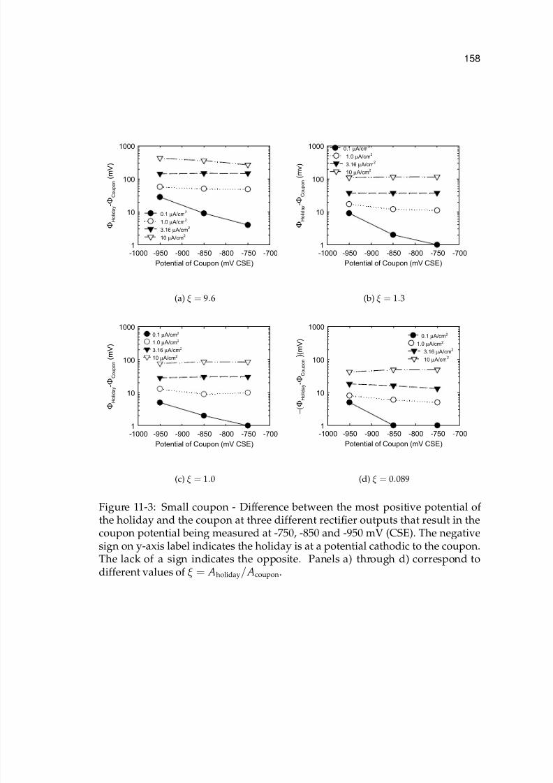
7/18/2019 Riemer PhD 2000


158


-1000 -950 -900 -850 -800 -750 -700

Φ H o l i d a y

- Φ C o u p o n

( m V )

1

10

100

1000

0.1 µ A/cm2

1.0 µ A/cm2

3.16 µ A/cm2

10 µ A/cm2

(a) ξ = 9.6


-1000 -950 -900 -850 -800 -750 -700

Φ H o l i d a y

- Φ C o u p o n

( m v )

1

10

100

1000 0.1 µ A/cm2

1.0 µ A/cm2

3.16 µ A/cm2

10 µ A/cm2

(b) ξ = 1.3


-1000 -950 -900 -850 -800 -750 -700

Φ H o l i d a y

- Φ C o u p o n

( m V )

1

10

100

10000.1 µ A/cm2

1.0 µ A/cm2

3.16 µ A/cm2

10 µ A/cm2

(c) ξ = 1.0


-1000 -950 -900 -850 -800 -750 -700

−

( Φ H o l i d a y

- Φ C o u p o n

) ( m V )

1

10

100

1000

0.1 µ A/cm2

1.0 µ A/cm2

3.16 µ A/cm2

10 µ A/cm2

(d) ξ = 0.089

Figure 11-3: Small coupon - Difference between the most positive potential of the holiday and the coupon at three different rectifier outputs that result in thecoupon potential being measured at -750, -850 and -950 mV (CSE). The negative

sign on y-axis label indicates the holiday is at a potential cathodic to the coupon.The lack of a sign indicates the opposite. Panels a) through d) correspond todifferent values of ξ = Aholiday/ Acoupon.

7/18/2019 Riemer PhD 2000


159

in the soil environment. An increase in ilim,O2 increased the difference between

the off-potential of the holiday and the off-potential of the coupon. The sign of

the differences given in Figures 11-2 and 11-3 determines whether the couponprovides a conservative assessment of the state of the holiday. For coupons that

are larger than the biggest holiday, the differences were negative, and the hol-

iday was more protected than the coupon. For coupons that are smaller than

the biggest holiday, the differences were positive, and the coupon was more pro-

tected than the holiday.

The ratio of holiday area to coupon area ξ =

Aholiday/ Acoupon is an importantparameter. While no specific critical value of ξ was found that gave consistently

conservative results, all coupons with ξ ≥ 1 over-predicted the level of cathodic

protection applied to the holidays. To compare the effects the geometry has on

the performance of the coupon, similar ratios of the holiday area to the coupon

area can be used. By comparing Figure 11.2(a) and Figure 11.3(b), one can see the

design of the smaller coupon, Figure 11.1(b), results in a slightly closer match to

the off potential of the holiday at high values of ilim,O2. As seen in Figure 11.3(a),

which represents a holiday with a surface area equal to the surface area of the

large coupon, the small coupon seriously over-predicted the level of cathodic

protection at the holiday. In this case, at high values of ilim,O2, the holiday po-

tential was very close to the corrosion potential for conditions where the small

coupon had an off-potential showing a 280 mV shift from the corrosion potential.

Ideally, a coupon should represent the off-potential of a holiday of similar

size. If the coupons did behave this way, then all the plots in Figures (11-2) and

(11-3) would have their lines at a 0 difference between the holiday and coupon at

7/18/2019 Riemer PhD 2000


160

Table 11.3: Results of two coupon model. The small coupon used a polarizationcurve with ilim,O2

= 1.0 µA/cm2 (curve 1). The large coupon used ilim,O2 that was

an order of magnitude smaller (curve 2).

Object Size Location Pol. Curve Pot. (CSE) Avg. Curr. Den.

Holiday 1 7.81 cm2 0o 1 -839 mV 1.11 µA/cm2





Small Coupon 9.36 cm2 122 cm 1 -850 mV 1.13 µA/cm2

Large Coupon 101 cm2 167 cm 2 -854 mV 0.241 µA/cm2

Table 11.4: Results of two coupon model. The large coupon used a polarizationcurve with ilim,O2 = 1.0 µA/cm2 (curve 1). The small coupon used a ilim,O2

thatwas an order of magnitude lower(curve 2).

Object Size Location Pol. Curve Pot. (CSE) Avg. Curr. Den.Holiday 1 7.81 cm2 0o 1 -867 mV 1.19 µA/cm2





Small Coupon 9.36 cm2 167 cm 2 -884 mV 0.356 µA/cm2

Large Coupon 101 cm2 122 cm 1 -850 mV 1.13 µA/cm2

all potentials. The results show that the coupon does not yield the off-potential

of a holiday of similar size. However, a linear relationship was found between

the difference between the off-potentials of the coupon and the holiday and the

mass transfer limited current density for oxygen reduction (ilim,O2). The ratio of

the surface areas then indicates whether holiday will be cathodic or anodic to the

coupon.

The results of the simulations for the multi-holiday, two-coupon system are

summarized in Tables 11.3 and 11.4. The results shown in Tables 11.3 and 11.4

7/18/2019 Riemer PhD 2000


161

simulate the use of coupons for a pipeline with a distribution of holiday sizes and

with the water table at the center-line of the pipe. Thus, the bottom of the pipe

is in wet soil, and the top of the pipe is dry. The least conservative assessmentof cathodic protection was obtained with the large coupon placed at the bottom

of the pipe (Tables 11.3). In this case, both coupons met the protection criterion

of −850 mV(CSE), yet only the smallest of the five holidays met the protection

criterion. The most conservative assessment of cathodic protection was obtained

with the large coupon placed at the top of the pipe (Tables 11.4). Again, both

coupons met the protection criterion of −850 mV(CSE). Only the largest of thefive holidays did not meet the protection criterion, and this holiday was only 35

mV short of -850 mV (CSE).

11.5 Coupon Performance Diagram

For cases where the polarization curves corresponding to electrochemical re-

actions on the coupon was the same as that on bare steel exposed by coating

holidays, the most important parameters were ξ = Aholiday/ Acoupon and iO2, the

current density for reduction of oxygen. All the calculated results could be placed

on a coupon performance diagram, shown in Figure 11.5. Cases where coupons

yield off-potentials more positive than exposed steel are indicated by black sym-

bols, cases where coupons yield off-potentials more negative than exposed steel

are indicated by open symbols, and cases where coupons yield off-potentials less

than 15 mV more negative than exposed steel are indicated by gray symbols.

Calculations to the left of the line at Aholiday/ Acoupon = 0.8 were considered

to yield conservative results. This can be interpreted as meaning that a coupon

7/18/2019 Riemer PhD 2000


162

0.1

1

10

0.01 0.1 1 10 100

Aholiday/Acoupon

i O 2 , µ A /

c m

2

Non-ConservativeConservative

Figure 11-4: Coupon performance diagram for coupons placed in the same soilenvironment as the pipeline coating defects that expose bare steel. The soil re-sistivity was 10,000 Ω cm. Black symbols correspond to calculations where aprotected coupon corresponded to a protected coating holiday. Open symbolscorrespond to calculations where the coupon could indicate adequate protectionfor pipes with coating holidays that are seriously underprotected. The gray sym-

bols correspond to cases where the coupon reading is not conservative, but theerror was less than 15 mV.

7/18/2019 Riemer PhD 2000


163

will yield a conservative assessment of the pipe condition so long as each coating

holiday that exposes bare steel exposes no more than 80 percent of the coupon

area. The dashed line indicates the approximate boundary for which the degreeto which the coupon was not conservative was smaller than 15 mV.

The position of these boundaries was a weak function of soil resistivity. An

increase in soil resistivity from 10,000 Ω cm to 100,000 Ωcm moved the position

of the solid boundary line from Aholiday/ Acoupon = 0.8 to 1.1.

Figure 11.5 did not provide a reliable indication of coupon performance for

cases where the polarization curve for the coupon corresponded to a less ag-gressive environment than that experienced by the bare steel exposed by coating

holidays. Coupons with an oxygen current an order of magnitude smaller than

that of the steel gave consistently non-conservative results, even for coupons with

areas 13 times the area of exposed steel. ( Aholiday/ Acoupon < 0.077).

It should be noted that the calculations presented here were for cases where

the only coating defects on the pipe exposed bare steel. The present work does

not address the use of coupons to assess the possible role of corrosion under intact

disbonded coatings.

11.6 Conclusion

To be useful for monitoring the health of pipelines under cathodic protection,

coupons should provide a conservative value such that the largest expected hol-

iday is protected when the coupon is protected. The present work shows that

the area of the coupon should be larger than the area of the largest expected

holiday. The performance of the coupon as a monitor of cathodic protection is

7/18/2019 Riemer PhD 2000


164

strongly influenced by the availability of oxygen in the soil. If coupons of differ-

ent sizes are to be used, the largest coupons should be placed in regions where

the mass-transfer-limited current density is largest. The sensitivity of the couponto the polarization curve indicates that coupons should be placed to sample all

soil environments encountered by the pipeline. If only one coupon is to be used,

it should be placed in the region of greatest oxygen availability. A coupon per-

formance diagram could be constructed which reveals conditions under which

a coupon yields a conservative assessment of cathodic protection to holidays ex-

posing bare steel. The coupon performance diagram addressed both polarization behavior and the relative size of coupons and coating holidays.

7/18/2019 Riemer PhD 2000


CHAPTER 12TANK BOTTOMS

Storage tanks are located at the terminus of most pipelines. They may be used

to store crude oil unloaded from ships, furnace fuel waiting for the fall demand,

or fuel depot reserves. Most cities have a fuel depot where gasoline, diesel, and

other types of petroleum products are stored before distribution to filling stations.

The storage facility allows pipelines to run continuously and efficiently, instead

of having to be turned on and off while filling individual delivery trucks.

Storage facilities usually consist of many above-ground storage tanks called

a tank farm. They are built of steel and rest on the soil. The tank bottom is then

subject to the same materials problems as the buried pipelines. As the geometry

of a tank is much different than pipelines, tanks have different problems with CP

design than do pipes. Since tanks sit on the ground and are operated at atmo-

spheric pressure, the steel is thinner (0.25”) and, therefore, low corrosion rates

can be catastrophic.117

Past tank failures and environmental problems have motivated installation

of underlying cache basins to prevent any leakage from entering the aquifer. The

liner of the cache basin is usually made of a very high dielectric membrane which

does not allow passage of electrical current. The CP systems for these types

of tanks are designed to place the anodes between the liner and the steel tank

bottom.118

165

7/18/2019 Riemer PhD 2000


166

Concentration profiles for oxygen under a storage tank are cyclic in nature.

The reason is that when the tank is empty, the center rises above the soil creating

a void. The void fills will air and because the tank is no longer in contact withthe soil, none of the oxygen in the soil at the center of the tank is consumed

through the oxygen reduction reaction (second term of equation (1-23)). When

the tank comes into contact with the soil again after filling, the mass-transfer-

limited current density for oxygen reduction is the same at the center as at the

periphery.

The model has been adapted to handle tank bottoms. It can also handle theinsulating cache basin if it is assumed that no current can pass through the liner

using the techniques derived in section 3.6.

12.1 Tank Bottom Mesh

The boundary element mesh for the tank bottom was created using isopara-

metric quadrilateral Lagrange elements and isoparametric quadratic triangles.67

The triangles are used to increase the degrees of freedom as the mesh proceeds

radially from the center. If the Lagrange elements where used exclusively, either

the center of the tank would be over-meshed, or the outside edge would have

a too-course mesh. The triangles are used to double the degrees of freedom by

placing a triangle at every other element on the last ring of elements that would

double the diameter from the previous spot where the number of degrees of free-

dom were doubled. Therefore, starting from the center, rings that use triangles

are 1 (the center which is all triangles), 2, 4, 8, 16, etc (see Figure 12-1). The den-

sity of elements is then set by specifying the density at the center and the total

7/18/2019 Riemer PhD 2000


167

Figure 12-1: High resolution mesh used for the boundary element mesh.

number of rings. The mesh generator takes care of the rest. The last ring is di-

vided into two rings to help handle the possible edge effects. The ring at the very

edge is 13

the size of the rest of the rings while the next to last is 23

the size.

Individual rings of elements were assumed to have the same parameters for

the polarization curve, equation (1-23). The axisymmetric setting of polarization

curve parameters does not mean that an individual ring will have the same po-

tential everywhere since different points in the rings can be at different points

on the polarization curve defined by the boundary condition parameters. It does

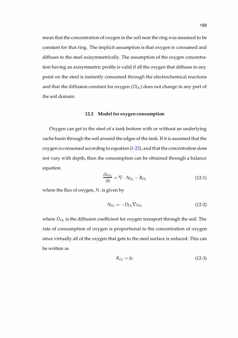
7/18/2019 Riemer PhD 2000


168

mean that the concentration of oxygen in the soil near the ring was assumed to be

constant for that ring. The implicit assumption is that oxygen is consumed and

diffuses to the steel axisymmetrically. The assumption of the oxygen concentra-tion having an axisymmetric profile is valid if all the oxygen that diffuses to any

point on the steel is instantly consumed through the electrochemical reactions

and that the diffusion constant for oxygen (DO2) does not change in any part of

the soil domain.

12.2 Model for oxygen consumption

Oxygen can get to the steel of a tank bottom with or without an underlying

cache basin through the soil around the edges of the tank. If it is assumed that the

oxygen is consumed according to equation (1-23), and that the concentration does

not vary with depth, then the consumption can be obtained through a balance

equation

∂ cO2

∂ t =∇ · N O2 − RO2 (12-1)

where the flux of oxygen, N , is given by

N O2 = −DO2

∇cO2 (12-2)

where DO2 is the diffusion coefficient for oxygen transport through the soil. The

rate of consumption of oxygen is proportional to the concentration of oxygen

since virtually all of the oxygen that gets to the steel surface is reduced. This can

be written as

RO2 = kc (12-3)

7/18/2019 Riemer PhD 2000


169

where k is the proportionality constant which accounts for the thin diffusion layer

next to the steel surface (on the order of 50 microns 41).

Substitution of equations (12-2) and (12-3) into (12-1) yields

∂ cO2

∂ t = −DO2

∇2cO2 − kc (12-4)

Under assumptions of a steady state and that oxygen concentration does not vary

with depth, equation (12-4) can be expressed in cylindrical coordinates as

Dd2c

dr2 +

D

r

dc

dr − kc = 0 (12-5)

Upon moving the constants into the last term and multiplying through by r2

r2 d2c

dr2 + r

dc

dr −

r

k

D

2

c = 0 (12-6)

which resembles a Bessel’s equation. To get the equation into the standard form

of Bessel’s equation, a variable transformation is made

ξ = r

k D (12-7)

where the derivatives are

dc

dr =

k

D

dc

dξ (12-8)

and

d2c

dr =

k

D

2d2c

dξ 2 (12-9)

Upon substituting equations (12-7), (12-8), and (12-9) into equation (12-6), the

modified Bessel”s equation of parameter 0 is obtained as

ξ 2d2c

dξ 2 + ξ

dc

dξ − ξ 2c = 0 (12-10)

7/18/2019 Riemer PhD 2000


170

whose solution is a modified Bessel function. The boundary conditions for the

original system in cylindrical coordinates are

at r = R, c = c∞ (12-11)

and

at r = 0, c is finite (12-12)

In the transformed coordinates, the boundary conditions become

at ξ = R k

D

, c = c∞ (12-13)

and

at ξ = 0, c is finite (12-14)

The solution to equation (12-10) is the modified Bessel function of the first kind.

It takes the form

c(ξ ) = AI 0(ξ )+ Bln(ξ )I 0(ξ )+∞∑

m=1 (−1)m−1

22m

(m!)2

m

∑n=1

1

n (12-15)

where A and B are constants to be determined from the boundary conditions.

Application of boundary condition (12-14) to equation (12-15) yields

c(ξ ) = AI 0(ξ ) (12-16)

Upon applying boundary condition (12-13),

c(ξ ) = c∞

I 0(R

k D

)I 0(ξ ) (12-17)

The solution is presented as a function of radial position in Figure 12-2 for several

values of the scaling parameter R

k /D.

7/18/2019 Riemer PhD 2000


171

0.00 0.25 0.50 0.75 1.00

c O 2

/ c O 2 , ∞

0.00

0.25

0.50

0.75

1.00

1= D

k R

5= D

k R

5.1= D

k R

2= D

k R

D

k R / ξ

Figure 12-2: Oxygen concentration profile within the soil at several values of the

scaling parameter R

k /D.

7/18/2019 Riemer PhD 2000


172

12.3 Implementation

The passage of current through the soil is governed by Laplace’s equation

which was solved using the boundary element method (BEM). The boundary

condition for the bare steel was given by equation (1-23). The anodes were also

allowed to be polarized according to equation (1-30).

The oxygen concentration distribution was applied through the boundary

condition at the steel surface of the tank bottom. The parameter, iO2 in equa-

tion (1-23) was adjusted according to equation (12-17). However, the value of

iO2 could only be adjusted in a step-wise manner. Each ring of elements in the

boundary element mesh was assigned a single value of the parameter (see Figure

12-1 for the element layout) which remained constant in that ring.

In addition to forcing a constant value of iO2 in each ring of elements, setting

a different value at each ring introduced an error at the edge of the ring in the

current density. The boundary element method compensates for the error at the

center of the element. Therefore the point at which to sample the solution is

critical for this type of simulation. The best points to sample are the Gauss points

for a 2x2 point rule (square parent element).119

There were three anode arrangements used corresponding to the three stan-

dard anode arrangements used in industry.120 The first was a remote ground-bed,

the second a distributed arrangement of 8 anodes placed around the circumfer-

ence of the tank and finally, ribbon anodes placed directly under the tank-bottom.

The remote ground-bed cannot be used when there is an insulating cache basin

under the tank.

7/18/2019 Riemer PhD 2000


173

12.4 Results

A single tank was modeled using the three anode arrangements described

above. The tank was 100 feet diameter with bare steel exposed to the soil. In

all cases the anode output was adjusted to 14.2 Amps. If the current density is

uniform for the entire tank-bottom, a protection level of 1.9 µA/cm2 would be

achieved which would cause the steel to be somewhat over-protected.

The possibility of an insulating cache under the electrolyte where the CP sys-

tem was installed was also modeled for the anode arrangements that can work

with it. The model could account for the soil surface or tank bottom and an op-

tional underlying insulator (see section 3.6).

The results are presented in a series of cases based upon the three possible

anode arrangements, starting with the remote ground-bed.

12.4.1 Remote Ground-bed

Smyrl and Newman provide a criterion for determining the maximum size

of tank that can be protected with a remote ground-bed without over-protection

assuming a uniform current density.121 The maximum radius is given by12

ro =∆Φoκ

0.363iavg(12-18)

where ∆Φo is the maximum over-polarization of the steel from the point of min-

imum protection (-850 mV CSE). If an undesirable rate of hydrogen evolution

takes place at -1200 mV CSE, then ∆Φo is equal to 350 mV. For an average current

density of 1.9 µA/cm2 and 10,000 Ωcm soil, the maximum radius is 51 cm. If the

7/18/2019 Riemer PhD 2000


174

soil resistivity is only 1000 Ωcm, then a tank of 5.1 m could be protected. A soil

resistivity significantly less than 10,000 Ωcm is not usually seen.

The current distribution on the tank bottom is not necessarily uniform but isexpected to be axisymmetric when a remote anode is used.121 The outermost ring

of the tank should have a much higher current density than the center if Tafel ki-

netics apply (hydrogen evolution).122 If the center of the tank is poorly polarized,

the net current density will be below the mass-transfer-limited current density for

oxygen reduction and again, the current density distribution is nonuniform.123

Therefore, it is not expected that equation (12-18) would be of much value for CPdesign. The polarization curve used in the model for bare steel can account for

each of the above possibilities.

The cathodic protection system was modeled using a deep well remote ground-

bed at 250 feet below the tank. The groundbed output was 14.2 Amps. It was

assumed that the soil resistivity was constant throughout the soil domain and

equal to 10,000 Ωcm. Two cases were calculated, one for the uniform oxygen con-

centration when the tank is filled, and one with an oxygen concentration profile

calculated from equation (12-17) to approximate the case when psudeo-steady-

state has been reached.

Uniform Oxygen Distribution The first calculation assumed a uniform con-

centration of oxygen in the soil to simulate the conditions that exist when the

tank has just been filled and the oxygen beneath the tank is not yet depleted. The

anode output was adjusted to 14.2 Amps. Equation (12-18) would predict the dif-

ference in potential between the outer edge and the center of the tank to be -10.5

volts if there is a uniform current distribution. Figure 12-3 shows the off-potential

7/18/2019 Riemer PhD 2000


175

Figure 12-3: Potential distribution when the oxygen concentration is uniform atits largest value. This condition occurs when the tank has been recently filledafter being empty. The grid spacing is 10 ft square.

distribution on the tank bottom. The center of the tank is at -605 mV Cu/CuSO4

or -75 mV from the corrosion potential which is 25 mV underprotected by the

-100 mV polarization shift criteria.124 The outside edge of the tank is polarized to

-1189 mV Cu/CuSO4, which is significantly more positive than the -10.5 volts pre-

dicted by equation (12-18). The potential variation is smaller because the current

density distribution was nonuniform, due to the role of corrosion and hydrogen-

evolution reactions. The value of -1189 mV is very close to -1200 mV Cu /CuSO4,

which is a point where hydrogen evolution is a significant concern.

Figure 12-4 shows the complete off-potential and current-density distribution

as a function of the radial position from the center of the tank. The current density

7/18/2019 Riemer PhD 2000


176

-1200

-1100

-1000

-900

-800

-700

-600

-500

0 0.2 0.4 0.6 0.8 1

r/r 0

O f f - P o t e n t i a l ( m V C

u / C u S O 4 )

0.1

1

10

100

i / i a v g

Figure 12-4: Radial potential and current density distribution when the oxygenconcentration is uniform and at c∞. Potential is given by the red line. The blackline indicates where a uniform current density distribution would be.

distribution is nearly equivalent to the primary distribution for a disk electrode

(see equation (7-1) on page 104). The value of J for the secondary distribution,

described by Newman,122 was equal to 536 (see equation (7-2) in section 7.1.2).

Thus, any small change in the current density at the center of the tank used to

increase the protection there, will result in significantly elevated current densities

at the edge of the tank. The more nonuniform current density distribution results

since increasing the average current density increases the value of J .

Nonuniform Oxygen Distribution As stated before, the solution to the oxygen

distribution under the tank was implemented by changing the value of the mass-

transfer-limited current density for oxygen reduction (iO2 ) to values predicted by

the solution to the diffusion equation for oxygen given in equation (12-17). The

profile for the oxygen distribution under the tank was taken using the scaling pa-

rameter, R

k /D, set to 2. The anode size and location was not changed for this

7/18/2019 Riemer PhD 2000


177

Figure 12-5: Potential distribution when the oxygen concentration follows the

profile given in Figure 12-2 corresponding to R

k /D = 2.0. The grid spacing is10 ft square.

simulation. The anode output was 14.2 Amps for the same potential setting as the

first simulation. The off-potential distribution is shown in Figure 12-5. This time,

the off-potential was much closer to being uniform. The polarization level at the

center was also significantly improved to -906 mV Cu/CuSO4. The corrosion po-

tential at the center, where it is most negative, was -550 mV Cu/CuSO4. Therefore

the center was polarized by over 350 mV. As one proceeds radially from the cen-

ter, the polarization level only increases. These results mean that the entire tank

was over-protected and money has been wasted by running the anode at too high

of a level.

7/18/2019 Riemer PhD 2000


178

-1200

-1100

-1000

-900

-800

-700

-600

-500

0 0.2 0.4 0.6 0.8 1

r/r 0

O f f - P o t e n t i a l ( m V C

u / C u S O 4 )

0.1

1

10

100

i / i a v g

Figure 12-6: Radial potential and current density distribution when the oxygenconcentration follows the profile given in Figure 12-2 corresponding to R

k /D =

2.0. Potential is given by the red line. The black line indicates where a uniformcurrent density distribution would be.

Figure 12-6 shows both the potential and current distribution for the nonuni-

form oxygen concentration profile. Again, the current distribution approached

the primary distribution and the total current was the same as before. The dif-

ference was in the potential distribution, especially at the center of the tank. A

substantial reduction in current could be safely made while still maintaining pro-

tection. However, as soon as the tank goes through a emptying/refilling cycle,

the current level would have to be increased again until the steady-state oxygen

concentration profile achieved.

12.4.2 Distributed Anodes

Another anode arrangement that can be used is shallow distributed anodes

where an arbitrary number of anodes are arranged in a circle around the outside

edge of the tank. The anodes are close to the surface so it may be possible to use

7/18/2019 Riemer PhD 2000


179

this configuration with an underlying insulating containment membrane. For

the following examples, 8 anodes were placed around the circumference of the

the same 100 ft diameter tank used in the previous 2 examples. The total outputof the anodes was set to match closely that of the previous two examples (14.2

Amps). The anodes were placed such that they were two feet from the edge of

the tank. The soil resistivity was set to 10,000 Ωcm.

Uniform Oxygen Distribution Figure 12-7 shows the potential distribution for

the tank when the oxygen concentration distribution is uniform. The center of the

tank was polarized only -16 mV from the corrosion potential as opposed to the

remote groundbed where the center was polarized by -75 mV at the same total

current. The corrosion current density was 0.57 µA/cm2 which is about half that

expected for unprotected general corrosion.

A plot of the current density is shown in Figure 12-8. Since the distributions

were no longer axisymmetric, the position that is selected for a plot of the distri-

butions is important. The distribution is periodic however, with one period being

the angular distance between two anodes. There are two possibilities for the plot,

select a line from the center to a point closest to any one anode, or select a line

from the center to a point between two anodes. For either case, where the pri-

mary distribution shows a value of i/iavg equal to 0.5 at the center of the tank, the

value for the distributed anodes is 0.25. Near the outside edge, there is a much

sharper turn in the distribution as it goes toward infinity even though the value

of J is the same as for the case with the remote groundbed ( J = 536). The corro-

sion current at the center of the tank is more than an order of magnitude higher

7/18/2019 Riemer PhD 2000


180

Figure 12-7: Potential distribution with distributed anodes and uniform oxygenconcentration profile. The distribution is must worse than the primary distribu-tion. The center is only polarized -16 mV

-1200

-1100

-1000

-900

-800

-700

-600

-500

0 0.2 0.4 0.6 0.8 1

r/r o


0.1

1

10

i / i a v g

Figure 12-8: Current density distribution on tank bottom with distributed anodesand uniform oxygen concentration profile. The distribution was taken on a linethat went from the center of the tank to a point on the edge exactly between twoanodes.

7/18/2019 Riemer PhD 2000


181

than that of the remote groundbed. In this case icorr,Fe is equal to 0.57 µA/cm2

compared to 0.0275 µA/cm2 for the remote ground bed protected tank.

The reason for the poor performance of the distributed anodes is geometry.The edge of the tank is significantly closer to the anodes than the center. There-

fore, is is much easier to drive current to the edge of the tank than to the center.

When a remote anode is used, all points on the tank are equally distant from the

anode.

Nonuniform Oxygen Distribution When distributed anodes were paired with

the nonuniform oxygen concentration distribution, the potential and current dis-

tributions obtained showed better protection at the center of the tank with the

was total current driven to the steel. The corrosion current is 3 orders of magni-

tude lower than when the oxygen concentration was uniformly high. The poten-

tial distribution on the tank is shown in Figure 12-9.

The potential and current density distribution are plotted in Figure 12-10. It is

interesting to note that the current density at the center of the tank was the same

as that for the uniformly high oxygen profile. The additional current needed to

reduce the extra oxygen for the case with the high oxygen profile comes from the

corrosion of the steel tank. Because the oxygen concentration was lower in the

present case, the same current density was better able to protect the metal.

Underlying Insulating Cache Basin with Uniform Oxygen Distribution If there

is an underlying electrically insulating layer such as a catch basin, remote ground-

beds cannot be used. Distributed anodes can be used with an underlying mem-

brane because they can be placed within the soil between the membrane and the

7/18/2019 Riemer PhD 2000


182

Figure 12-9: Potential distribution with distributed anodes and nonuniform oxy-gen concentration profile. The distribution is much worse than the primary dis-tribution.

-1200

-1100

-1000

-900

-800

-700

-600

0 0.2 0.4 0.6 0.8 1

r/r o

O f f - P o t e n t i a l ( m V C u / C u S O

4 )

0.1

1

10

i / i a v g

Figure 12-10: Potential and current density distribution on a tank bottom withdistributed anodes and nonuniform oxygen concentration profile. The distribu-tion was taken on a line went from the center of the tank to a point on the edgeexactly between two anodes.

7/18/2019 Riemer PhD 2000


183

Figure 12-11: Potential distribution with distributed anodes, underlying insulat-ing layer at 2 ft and uniform oxygen concentration profile. The distribution is theworst of all the examples even though all examples have the same total current

being driven to the tank bottom. The center of the tank is polarized -13 mV fromthe corrosion potential.

tank. As might be expected the situation is worse than if the insulating layer did

not exist. The reason to expect poorer performance is that there are significantly

fewer current paths from the anode to the center of the tank due to the narrow

layer of soil in which the current must flow. There should also then be an increase

in the current density at the edge of the tank.

Figure 12-11 shows the potential distribution for a tank protected in such a

manner. The center of the tank was polarized only -13 mV from the corrosion

potential which is about 25% less than the case without the insulating cache basin.

Therefore, intuition has served well. The current density at the center of the tank

was 15% less than when there was no cache.

7/18/2019 Riemer PhD 2000


184

Figure 12-12: Potential distribution with distributed anodes, underlying insulat-ing layer at 2 ft and nonuniform oxygen concentration profile. The center of thetank is polarized -80 mV from the corrosion potential.

Underlying Insulating Layer with Nonuniform Oxygen Distribution When

the oxygen at the center of the tank has been consumed, the polarization im-

proves significantly, but not to a required level. The center of the tank was only

polarized by -80 mV. The remote groundbed with no cache basin was able to po-

larize the center of the tank by -350 mV. The potential distribution is shown in

Figure 12-12. Again, the current density distribution was nearly identical for the

two cases with an insulating cache liner.

12.4.3 Ribbon Anodes

A third method of applying cathodic protection is to use ribbon anodes placed

very close to the tank-bottom. The ribbon configuration can yield a more uniform

current distribution. Two anode arrangements were used for the evaluation of

7/18/2019 Riemer PhD 2000


185

(a) Mesh for 5 Ribbons (b) Mesh for 11 Ribbons

Figure 12-13: Tank bottom with 5 and 11 parallel impressed current anodes. Thegray grid lines are on 10 ft intervals. The tank with 5 anodes uses 4 inch diameteranodes and the one with eleven uses 1 inch diameter ribbons. The mesh for thetank with 11 ribbons is more refined.

ribbons. The first used 5 parallel impressed current ribbons of 4 inch diameter,

the second used 11 1 inch anodes in a similar configuration. The setup for the

two cases is shown in Figure 12-13.

The mesh for the tank that had 11 anodes was made to be finer than the one

which had 5 anodes. A finer mesh was used to provide a reasonable level of

detail with the more closely spaced anodes, since there would not even be an axi-

periodic distribution seen with the distributed anodes. The anodes were assumed

to be cylindrical and were discretized in both the axial and angular directions.

The angular discretization could then account for the nonuniform current and

potential distribution due to the proximity of the tank.

7/18/2019 Riemer PhD 2000


186

(a) 5 Ribbons (b) 11 Ribbons

Figure 12-14: Potential distribution for tank bottoms with 5 and 11 parallel im-pressed current anodes with secondary containment. The gray grid lines are on10 ft intervals. Peak corrosion rate for tank with 5 anodes is an order of magni-tude higher than that of the tank with 11 anodes. Total current driven to tank is14.2 Amps for both cases.

Uniform Oxygen Distribution with Insulating Cache Basin For both anode

design cases, the total current output to the tank bottom was adjusted to 14.2

Amps. The potential distributions for the two systems are shown in Figure 12-

14. The peak corrosion current for the tank with 5 anodes was 1.6 µA/cm2. This

large value, higher than could be expected from oxygen reduction alone, was due

to galvanic coupling between the highly polarized metal that is very close to an

anode and the poorly polarized metal between the anodes. Poorly polarized re-

gions are shown in red in Figure 12.14(a) and highly polarized regions are coloredin blue. The same color scheme and scale are used in Figure 12.14(b). Here the

potential distribution was much better, but not yet optimal, even though the an-

ode surface area was half that of the example with 5 anodes. The anode-to-anode

7/18/2019 Riemer PhD 2000


187

distance was cut in half with the 11 anode system. The result is that 25% smaller

driving force was needed to drive the same amount of current to the tank bottom,

even with the reduced area of the anodes.

Uniform Oxygen Distribution without Insulating Cache Basin When the in-

sulating cache basin was removed, some unexpected phenomena were observed

while adjusting the impressed current setting in order to drive 14.2 Amps to the

tank surface. It was estimated that roughly the same driving force would be

required to achieve the same current levels as was used for the cases using the

insulating cache. It was found, instead, that a substantial increase in driving force

was needed to obtain the same total current. To understand why there is such a

large disparity between the two systems, even though the anodes are identical, it

helps to look at the current density distribution along the length of the anodes.

The axial current density distribution for the long center anode for both the 5 and

11 anode cases is shown in Figure 12-15. In both cases, when there is no electrical

insulator under the the anodes, most of the current comes from either end. The

effect of more nonuniform current density distribution is to require a great deal

more voltage to drive the same total current.

The current density and corrosion current distribution for the worst case of

the 5 ribbons is shown in Figure 12-16 The largest corrosion current is next to the

long center ribbon at either end. There is evidence of galvanic coupling about

two-thirds of the distance from the center of the tank to the edge. The corro-

sion current density is about 2 µA/cm2 which is double the rate due to general

corrosion.

7/18/2019 Riemer PhD 2000


188

10

100

1000

10000

0 20 40 60 80 100Position (ft)

C u r r e n t D e n s i t y

( µ µ µ µ A / c m

2 ) Without Insulating Cache Basin

With Insulating Cache Basin

(a) 5 Ribbons

10

100

1000

10000

0 20 40 60 80 100

Position (ft)

C u r r e n t D e n s i t y ( µ µ µ µ A / c m

2 ) Without Insulating Cache Basin

With Insulating Cache Basin

(b) 11 Ribbons

Figure 12-15: Axial current density distributions on anodes for both the 5 and11 anode cases. For each case, the current density distribution is plotted for thesituations of having an insulating cache basin and only having conductive soilunder the tank.

(a) 5 Ribbons (b) 5 Ribbons (Corrosion current)

Figure 12-16: Potential and corrosion current distribution for tank bottoms with5 parallel impressed current anodes with no secondary containment. The graygrid lines are on 10 ft intervals. Total current driven to tank is 14.2 Amps. Thereare significantly more anodic sections in this case with 5 anodes than for the casewith an insulating cache basin.

7/18/2019 Riemer PhD 2000


189


Figure 12-17: Potential distribution for tank bottoms with 5 and 11 parallel im-pressed current anodes and secondary containment with nonuniform oxygen dis-tribution. The gray grid lines are on 10 ft intervals. Total current driven to tankis 14.2 Amps for both cases. Center of tank is more polarized than in the caseshown in Figure 12-14

Nonuniform Oxygen Distribution with Insulating Cache Basin The case of

a nonuniform oxygen concentration profile was modeled for both the 5 and 11

anode CP systems. The anodes were again adjusted such that the total output

was 14.2 Amps. The potential distributions are shown in Figure 12-17. As ex-

pected, the center of the tank was polarized to a more negative potential then

that shown in Figure 12-14. The current distribution was nearly identical to that

of the uniform oxygen case.

Nonuniform Oxygen Distribution without Insulating Cache Basin The last

case involved removing the restriction of the underlying insulating cache. The

7/18/2019 Riemer PhD 2000


190


Figure 12-18: Potential distribution for tank bottoms with 5 and 11 parallel im-pressed current anodes and no secondary containment with nonuniform oxygendistribution. The gray grid lines are on 10 ft intervals. Total current driven totank is 14.2 Amps for both cases.

potential distribution is shown in Figure 12-18. In this case, the center of the tank

was not as well polarized as in the case where the cache basin is present. Again,

the absence of a catch basin caused a more nonuniform current distribution on

the anodes. The current density was much lower at the centers of the anodes than

it was with the cache membrane present. To compensate, the current density was

higher at the ends of the anodes which, then, promoted a larger current density

at the edge of the tank. The current was better distributed than when remote or

distributed groundbeds were used.

Use of larger numbers of ribbons also served to improve the current distribu-

tion for all cases where ribbons were used. If the spacing was too large, there was

a possibility of galvanic coupling between the sections of the tank that were more

7/18/2019 Riemer PhD 2000


191

polarized directly above the anodes and sections in between the anodes. For the

100-ft diameter tank bottom used in the examples, it appears that a 10-ft spacing

between parallel ribbons represents an upper bound.

12.5 Conclusions

Even under the best of situations, it is very difficult to provide cathodic pro-

tection to the centers of tank bottoms. If remote anodes or anodes distributed

around the circumference of the tank are used for protection, the best that can be

hoped for is a current distribution that approaches the primary as given in equa-

tion (7-1). In the case of distributed anodes around the perimeter, the situation

is much worse than for the remote ground-bed. Because of the proximity of the

anodes to the outside edge of the tank, most of the current goes to polarizing the

edge of the tank.

The only solution that can work is to place anodes directly under very close

to the steel they are to protect. Design of such systems is required. If the spacing

between anodes is too great, anodic regions can form on the steel between the

anodes. The goal should also be to provide the largest amount of anode surface

area possible to reduce to driving force needed to supply a sufficient total current

to the tank. With a smaller driving force, there is significantly less likelihood of

anodic regions forming on the tank bottom steel.

Cyclic oxygen concentration gradients along the tank bottom due to periodic

emptying and filling of the tank can cause periodic over- and under-protection.

Therefore, it may be important to include reference electrodes in the design of the

CP system to monitor the polarization of the steel.

7/18/2019 Riemer PhD 2000


192

The location of the reference electrode is very dependent on the design of the

CP system. If the design uses remote ground-beds, or a distributed ground-bed

around the circumference of the tank, is is most important to monitor the centerof the tank. Other design require modeling of the design to determine optimal

locations. As shown in Figure 12-14 the optimal location is not at the center of

the tank but near the longest ribbon about 3/4 of the distance from the center to

the edge of the tank.

When a nonuniform oxygen distribution occurs, the parallel ribbon type an-

ode system cannot be adjusted at the center of the tank. A high level of polariza-tion occurs at the center because of the lack of controlability. A new design for

the anode layout has been proposed by Koszewski.118 The arrangement consists

of individually controlled concentric ring anodes. Unfortunately, the model does

not have the ability to create curved anodes.

In the end, it was quite by accident that the best means of properly protecting a

tank bottom was found. By restricting the current paths, the lining plays an active

role in cathodic protection design and forces a more uniform current distribution

on the tank bottom. The requirement of the Environmental Protection Agency

that all new tanks have secondary containment was designed to contain spills,

but may have also resulted in an optimal CP design.125

7/18/2019 Riemer PhD 2000


CHAPTER 13MULTIPLE SOIL DOMAINS

One of the assumptions made in deriving the governing differential equations

in Chapter 2, was that the ionic strength of the electrolyte within the domain

was constant. Many times, however, it may be desirable to relax that restriction.

Changes in soil resistivity may need to be considered, for example, at a river

crossing where a pipe passes through a section of water saturated soil.

Greens function solutions for these types of problems are very difficult to ob-

tain. There have been some solutions reported61 for the case when the conductiv-

ity is a linearly varying function in only one of the three dimensions. However,

to use this solution, a region of constant conductivity must be placed on either

side of the region with the linear variation. If one does not do this, then one end

of the region will have a negative conductivity which has no physical meaning

while the extreme other end will have near superconducting characteristics. If a

Green’s function cannot be used, the only alternative for the boundary element

method is to divide the domain into regions. At the point of division between

regions, a mesh must be created which adds to the computational load.

13.1 Continuity Equations

Often, such as at river crossings, the change in soil conductivity is abrupt and

can be modeled as a plane. Figure 13-1 shows how the division must be modeled

using the boundary element method. The point of the change in soil properties is

193

7/18/2019 Riemer PhD 2000


194

Figure 13-1: Plane meshed for a soil type change. Three pipes are shown passingthrough a point where the soil conductivity changes.

7/18/2019 Riemer PhD 2000


195

assumed to be a plane. The plane is then meshed since it is a boundary between

two domains of constant conductivity. The two domains must then be coupled

together through the common boundary of the mesh at the soil type division.If steady state is assumed, then there can be now accumulation of charge on any

arbitrary plane within a domain governed by Laplace’s equation.68 Therefore, the

continuity of current through the plane is given by

κI ( n · ∇ΦI ) =−κI I ( n · ∇ΦI I ) (13-1)

where κ is the soil conductivity, n is the normal vector, and Φ is the potential on

either side of the division. The reason for allowing separate values of potential on

either side of the division is due to a phenomenon known as the liquid junction

potential.12 A liquid junction potential arises when there is a difference in ionic

strength at either side of a junction and a difference in diffusion coefficients be-

tween the anions and cations. The change in potential can be calculated through

the Henderson formula if the concentrations and diffusion coefficients for all the

charged species are known. The continuity condition at the soil division becomes

ΦI = ΦI I +ΦLJ (13-2)

where ΦLJ is the liquid junction potential. Careful attention must be paid to the

sign of the liquid junction potential.

13.2 Implementation

Soil divisions are implemented within the boundary element method only.

Laplace’s equation is written for each domain which is now bounded by the soil

7/18/2019 Riemer PhD 2000


196

surface (see section 3.5), and one or two soil type division half-planes. Then a set

of algebraic equations from equation (4-1) can be written for for the first domain

H j, j H j,i H i, j H i,i

Φ j

Φi

= G j, j G j,i

Gi, j Gi,i

n · ∇Φ j

n · ∇Φi

(13-3)

where i represents nodes and elements on the soil division interface and j is for

all other nodes and elements within the domain. The second domain would be

written as

H i,i H i,k

H k ,i H k ,k

Φi

Φk

= Gi,i Gi,k

Gk ,i Gk ,k

n

· ∇Φi

n · ∇Φk

(13-4)

where i again represents nodes and elements on the same boundary as in equa-

tion (13-3) and k represents all nodes and elements not on the domain boundary

and within domain two. Applying the continuity conditions from equations (13-

1) and (13-2) results in

H j, j H j,i 0

H i, j H i,i,1 + H i,i,2 H i,k

0 H k ,i H k ,k

Φ j

Φi

Φk

=

G j, j G j,i 0 0

G j, j Gi,i,1 − κ1

κ2Gi,i,1 Gi,k −∑ H i,i,2

0

−κ1

κ2Gk ,i Gk ,k 0

n · ∇Φ j

n · ∇Φi

n · ∇Φk

ΦLJ,1−2

(13-5)

where the subscripts 1 and 2 refer the the domain the matrix elements come from

and ΦLJ,1−2 comes from the liquid junction potential between domains 1 and 2

calculated using the Henderson formula. If there are n domains in the problem

7/18/2019 Riemer PhD 2000


197

then n − 1 extra columns are added to the right-hand matrix to account for liquid

junction potentials.

13.3 Steel Resistance in Multiple Soil Domains

The equations for the conduction of current through the pipe steel, bonds and

anodes is solved exactly the same as described in section 3.7. The only caveat

is that there are no entries in the finite element matrices for the soil domain divi-

sions since they are not part of the steel domain where the FEM is applied. Again,

the variable transformation described in section 4.9 is used to obtain

0 0 H j, j H j,i 0 −4π

0 0 H i, j H i,i,1 + H i,i,2 H i,k −4π

0 0 0 H k ,i H k ,k −4π

K j 0 K j 0 0 0

0 K k 0 0 K k 0

0 0 0 0 0 0

Ψ j

Ψk

Φ j

Φi

Φk

Φ∞

=

G j, j G j,i 0 0

G j, j Gi,i,1 − κ1


0 −κ1

κ2Gk ,i Gk ,k 0

ˆ F j 0 0 0

0 0 ˆ F k 0

A j 0 Ak 0

n · ∇Φ j

n · ∇Φi

n · ∇Φk

ΦLJ,1−2

(13-6)

Many domains can be strung together using the above method. Figure 13-

2 shows how the mesh for a system with two soil divisions and therefore three

different soil types. This model setup may be appropriate for a situation where

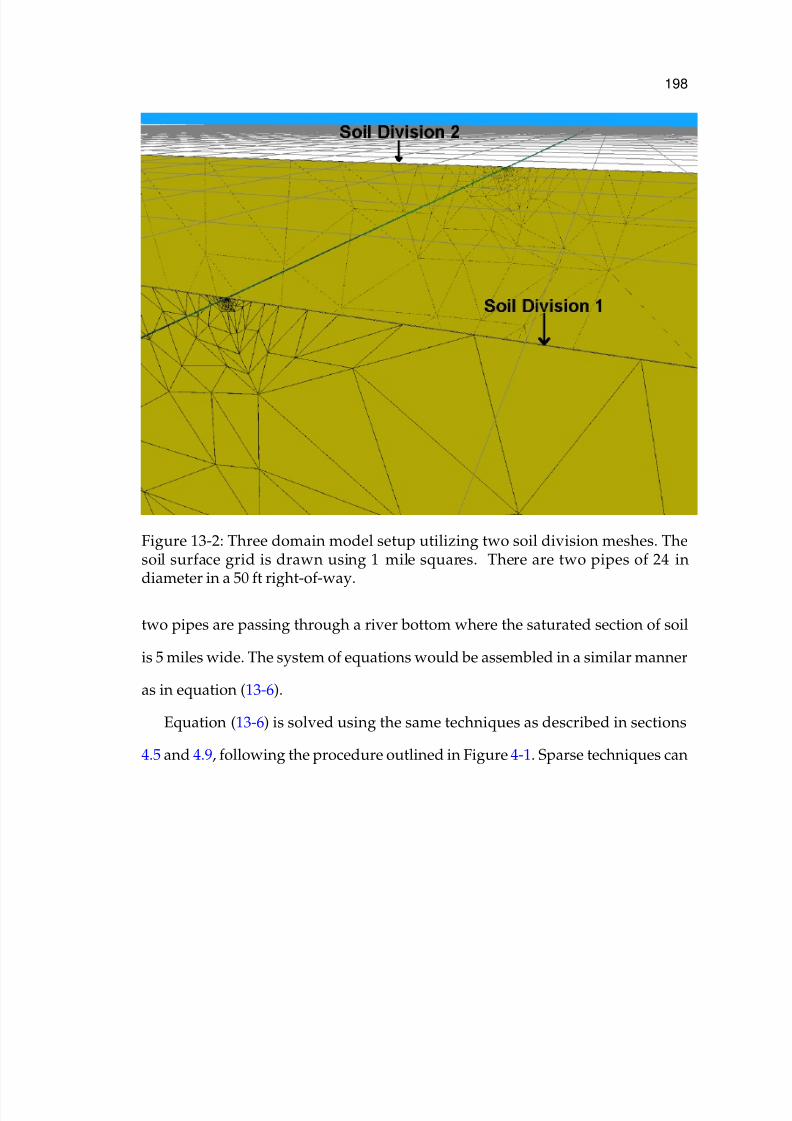
7/18/2019 Riemer PhD 2000


198

Figure 13-2: Three domain model setup utilizing two soil division meshes. Thesoil surface grid is drawn using 1 mile squares. There are two pipes of 24 indiameter in a 50 ft right-of-way.

two pipes are passing through a river bottom where the saturated section of soil

is 5 miles wide. The system of equations would be assembled in a similar manner

as in equation (13-6).

Equation (13-6) is solved using the same techniques as described in sections

4.5 and 4.9, following the procedure outlined in Figure 4-1. Sparse techniques can

7/18/2019 Riemer PhD 2000


199

be used to solve equation (13-6) if the variables are reordered to

H j, j H j,i 0 0 0 −4π

H i, j H i,i,1 + H i,i,2 H i,k 0 0 −4π

0 H k ,i H k ,k 0 0 −4π

K j 0 0 K j 0 0

0 0 K k 0 K k 0

0 0 0 0 0 0

Φ j

Φi

Φk

Ψ j

Ψk

Φ∞

=

G j, j G j,i 0 0

G j, j Gi,i,1 − κ1


0 −κ1

κ2Gk ,i Gk ,k 0

ˆ F j 0 0 0

0 0 ˆ F k 0

A j 0 Ak 0

n · ∇Φ j

n · ∇Φi

n · ∇Φk

ΦLJ,1−2

(13-7)

Sparse techniques cannot usually be used with mixed boundary condition prob-

lems under the formulation shown in equation (13-7). After all of the unknown

boundary conditions are moved to the left-hand-side, many elements in the the 0

submatrices above the K submatrices are filled with G submatrices. When non-

linear boundary conditions are used, many of the remaining terms with zeros in

the upper triangle above the K submatrices are filled with terms from the partial

derivatives of the boundary conditions when the Newton-Raphson technique is

implemented. The resulting matrices will not be sparse.

7/18/2019 Riemer PhD 2000


CHAPTER 14CONCLUSIONS AND FUTURE WORK

14.1 Conclusions

Buried pipelines carry most of the United States’ natural gas and petroleum

products from wells to refineries and to final consumption points. All of the

pipes are subject to corrosion and therefore have cathodic protection systems to

protect them. To reduce the amount of current required to protect the pipes,

high-resistivity coatings have been applied to the pipes. Coating defects expose

portions of bare steel to the soil environment, and cathodic protection is conse-

quently employed as a secondary measure. New mathematical models are re-

quired because the standard design equations cannot account for the behavior

of the cathodic protection system when coating defects are present. The design

of cathodic protection systems has been further complicated as demand has in-

creased because new pipes have been placed next to old pipes in the same right-

of-ways.

A numerical model has been developed to address the need to understand

how cathodic protection systems behave in the complicated installations found

today. New methods for treating the coating have been developed to predict

more accurately the protection levels of coated pipes with holidays. Complete

axial and angular current density and potential distributions can now be calcu-

lated for complicated pipeline networks.

200

7/18/2019 Riemer PhD 2000


201

Interactions between pipes with coating holidays have been shown in Chapter

10. Coating holidays produce a substantial “shadowing” effect on neighboring

pipes.It has been shown that the model can easily be extended to geometries other

than pipes through the investigation of cathodic protection of tank bottoms. Through

the investigation, it was shown how a fundamental understanding of potential

and current distributions can influence the design of CP systems.

14.2 Future Work

The largest weakness of the model is the lack of good polarization data for

both the bare and coated steel. Polarization parameters are strong functions of

steel composition and pre-treatments, soil environment, time, and history. Ken

Jeffers introduced a technique that could be used to provide high-quality, time-

dependent parameters for the polarization curves.41

Incorporation of time-dependent polarization curves requires that the model

be modified to integrate the time evolution of the system. Because the bound-

ary conditions are time-dependent, additional derivations are needed. One at-

tempt has been made by Santiago and Telles.126, 127 They incorporated the time-

dependent polarization curves for sea-water proposed by Nisancioglu.20 Steve

Carson has provided data for a similar formulation of the polarization curves for

pipes in soil environments.128

The model can be easily extended to other applications. For example, ship

hulls can be treated in a similar manner as pipes. The major modification needed

is to provide a means to mesh the geometry of the hull and propellers, and to

7/18/2019 Riemer PhD 2000


202

provide polarization curves for the metals used in their construction. Wells could

also be treated if a technique is available to account for the multiple soil layers

the well passes though. One method may be to use the techniques described inChapter 13. The domain divisions normal to the soil surface would be replaced

by divisions parallel to the soil surface.

Cathodic protection of the interior of pipes, storage tanks, reactor vessels, heat

exchangers can also be treated with some simple changes to the formulation. In

all cases, high-quality polarization data would be needed for the specific envi-

ronments.

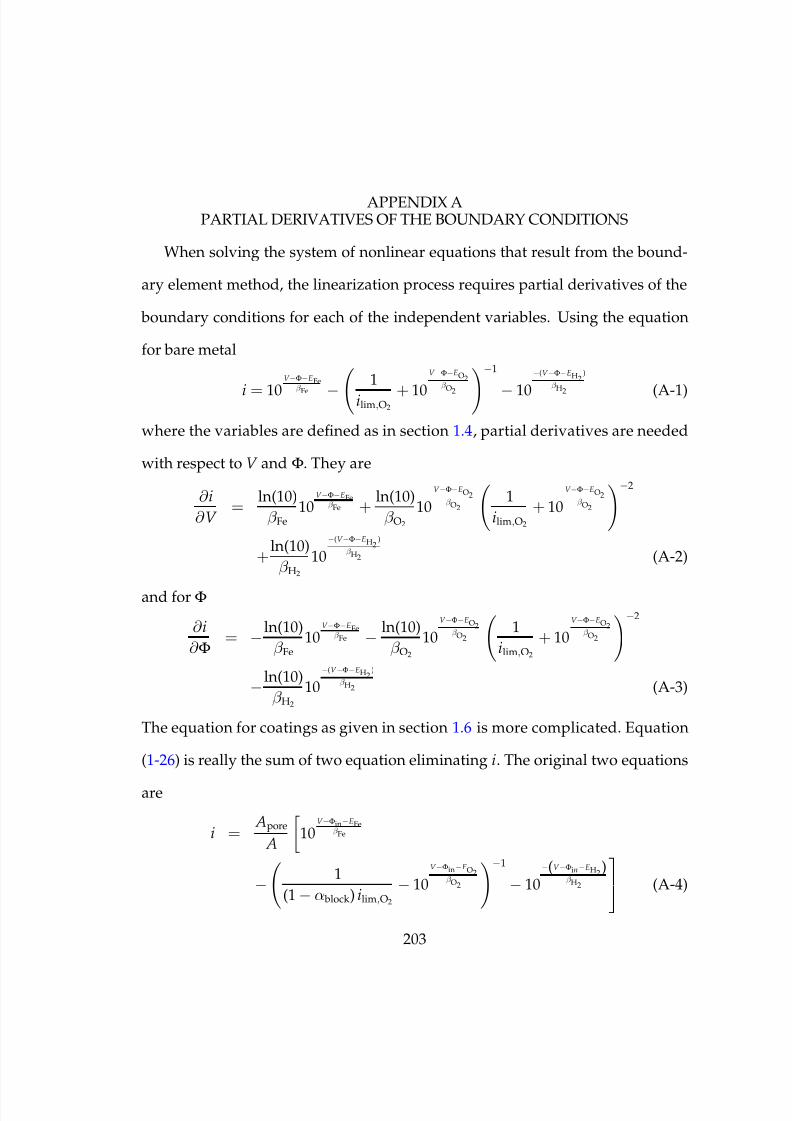
7/18/2019 Riemer PhD 2000


APPENDIX APARTIAL DERIVATIVES OF THE BOUNDARY CONDITIONS

When solving the system of nonlinear equations that result from the bound-

ary element method, the linearization process requires partial derivatives of the

boundary conditions for each of the independent variables. Using the equation

for bare metal

i = 10

V −Φ−EFeβ

Fe − 1

ilim,O2+ 10

V −Φ−EO2β O

2−1

− 10

−(V −Φ−EH2)

β H2 (A-1)

where the variables are defined as in section 1.4, partial derivatives are needed

with respect to V and Φ. They are

∂ i

∂ V =

ln(10)

β Fe10

V −Φ−EFeβ Fe +

ln(10)

β O2

10

V −Φ−EO2β O2

1

ilim,O2

+ 10

V −Φ−EO2β O2

−2

+ln(10)

β H2

10

−(V −Φ−EH2)

β H2 (A-2)

and for Φ

∂ i

∂ Φ = − ln(10)

β Fe10

V −Φ−EFeβ Fe − ln(10)

β O2

10

V −Φ−EO2β O2

1

ilim,O2

+ 10

V −Φ−EO2β O2

−2

− ln(10)

β H2

10−(V −Φ−EH2

)

β H2 (A-3)

The equation for coatings as given in section 1.6 is more complicated. Equation

(1-26) is really the sum of two equation eliminating i. The original two equations

are

i = Apore

A

10

V −Φin−EFeβ Fe

−

1

(1 − α block) ilim,O2

− 10

V −Φin−EO2β O2

−1

− 10

−(V −Φin−EH2 )β H2

(A-4)

203

7/18/2019 Riemer PhD 2000


204

and an IR drop

i =Φ−Φin

ρfilmδ film(A-5)

Equations (A-4) and (A-5) are solved simultaneously to get the current density i

using a Newton-Ralphson technique. The partial derivatives

∂ i

∂ Φ (A-6)

and

∂ i

∂ V (A-7)

are obtained numerically.

Numerical differentiation is done with a central difference formula

∂ i

∂ Φ =

i(Φ+ h, V ) − i(Φ+ h, V )

2h (A-8)

where h is a small number. The size of h must be carefully chosen such that

i(Φ+ h, V ) − i(Φ+ h, V ) is not equal to zero because h is smaller than the noise

due to finite machine precision and i(Φ+ h, V ) − i(Φ+ h, V ) does not straddle

large variations in the function. The value of h is selected based on the mag-

nitude of the variable it is modifying, i.e., Φ. The value of the machine , the

smallest number added to 1 such that the result is different than 1, is used to find

h according to

h = max(Φ, 1.0)√

(A-9)

In general, Φ is on the order of 1 Volt.

7/18/2019 Riemer PhD 2000


APPENDIX BOpenGL CODE

OpenGL R∗ was used for the rendering of graphics for the model.102 The draw-

ing commands are platform independent, so code that utilizes OpenGL can easily

be ported across different platforms. The only caveat is that the OpenGL device

setup is not platform independent. The reason is that windows are created in dif-

ferent ways depending on the platform, i.e., XWindows, Macintosh,† Windows

NT,‡ Iris,§ Solaris,¶ AIX, etc. Therefore, a small subset of code written by the

operating system manufacturer must be used to initialize the OpenGL device.

B.1 The OpenGL Device

The OpenGL device on the Windows NT platform must be created and at-

tached to a window before any drawing commands are issued. The device is

created during the window creation subroutine. As soon as the operating system

has created a generic window, a Pixelformat is specified for the OpenGL device

based of the capabilities of the window. Once the the Pixelformat has been suc-

cessfully chosen, the rendering device is created and attached to the window

∗OpenGL is a registered trademark of Silicon Graphics, Inc.†Macintosh is a registered trademark of Apple Computers, Inc.‡Windows NT is a registered trademark of Microsoft Corp.§Iris is a registered trademark of Silicon Graphics, Inc.¶Solaris is a registered trademark of Sun Microsystems, Inc.AIX is a registered trademark of IBM, Inc.

205

7/18/2019 Riemer PhD 2000


206

through the wglCreateContext command. Since only a single OpenGL con-

text may be active at any given time, a command is given to the new context to

make it the current one. The command must be issued every time a drawing cy-cle begins. Source listing B.1 contains the code used to set up the OpenGL device

for the model.

Source Listing B.1: OpenGL window setup code.

int CObjView::OnCreate(LPCREATESTRUCT lpCreateStruct)

2

// create the window

4 if (CView::OnCreate(lpCreateStruct) == -1)

return -1;

6

// get the windows drawing device

8 m_pDC=GetDC();

10 // get pixel formats

PIXELFORMATDESCRIPTOR PixFormat;

12

// zero out the pixel format

14 memset(&PixFormat, 0, sizeof(PIXELFORMATDESCRIPTOR));

16 //set some desired variables

PixFormat.nSize=sizeof(PIXELFORMATDESCRIPTOR);18 PixFormat.dwFlags=PFD_DRAW_TO_WINDOW |

PFD_SUPPORT_OPENGL | PFD_DOUBLEBUFFER ;

20 PixFormat.nVersion=1;

PixFormat.iPixelType=PFD_TYPE_RGBA;

22 PixFormat.cDepthBits=32; // the z-buffer

PixFormat.iLayerType=PFD_MAIN_PLANE;

24 // now choose the nearest format to the

// above modification

26 int rVal=ChoosePixelFormat(m_pDC->GetSafeHdc(),

&PixFormat);

28 if(rVal==0)return -1;

30

// now set the pixformat for this view using

32 // the just returned index

if(!SetPixelFormat(GetDC()->GetSafeHdc(), rVal,

34 &PixFormat))

7/18/2019 Riemer PhD 2000


207

36 // failed to set the pixel format

AfxMessageBox("Failed to set the pixel

38 format. Be sure that OpenGL is installed");

return -1;40

42 // check if a 256 color palate must be created

DescribePixelFormat(m_pDC->GetSafeHdc(), rVal,

44 sizeof(PIXELFORMATDESCRIPTOR), &PixFormat);

46 if(PixFormat.dwFlags & PFD_NEED_PALETTE)

GetOpenGLPalette();

48

// now set the rendering context

50

m_hGLRC = wglCreateContext(GetDC()->GetSafeHdc());if(m_hGLRC==NULL)

52 return -1;

54 //make it the current context

if(wglMakeCurrent(GetDC()->GetSafeHdc(),m_hGLRC)==FALSE)

56 return -1;

58 // one time Device setup parameters are also set here

60 // white background

glClearColor(1.0f,1.0f,1.0f,1.0f);

62 // color properties of materials will be used

glEnable(GL_COLOR_MATERIAL );

64

// materials only on front of face, ambient color may change

66 glColorMaterial(GL_FRONT, GL_AMBIENT);

68 glEdgeFlag(TRUE);

// polygons are numbered counterclockwise

70 glFrontFace(GL_CCW);

// dont draw faces that face away from the viewer

72 glCullFace(GL_BACK);

glClearDepth( 1.0 );74 return 0;

Line 4-47 are used to determine the number of colors OpenGL will use. The

command to create the device is in line 50.

7/18/2019 Riemer PhD 2000


208

B.2 The Drawing Cycle

The drawing cycle begins with a message from the operating system or from

the interactive code written by the programmer that says something within the

window has changed and it needs to be redrawn. The first step is to make the

windows OpenGL device the current one so that drawing commands are not

sent to the wrong window. Next all the platform independent OpenGL drawing

code is called. Finally SwapBuffers is called to place all the newly rendered

objects into the window. The code below in source listing B.2 demonstrates the

procedure.

Source Listing B.2: Draw command called by operating system whenever a win-dow needs updating.

void CObjView::OnDraw(CDC* pDC)

2

// get the size of the window

4 CRect rect;

GetClientRect(&rect);

6

// get a handle to the current device so that it

8 // can be restored when we are finished

HDC hOldDC = wglGetCurrentDC();

10 HGLRC hOldRC = wglGetCurrentContext();

12 // make this windows devide the current device

wglMakeCurrent( pDC->GetSafeHdc(), m_hGLRC );

14

// create the 3-D fonts if they have not been

16 CFont *pOldFont=pDC->SelectObject(m_pFont);

if(m_bBuildFont)

18

wglUseFontBitmaps (pDC->GetSafeHdc(), 0, 255, 1000);

20 m_bBuildFont=FALSE;

22 // Set the pointer to where the fonts are stored

glListBase (1000);

24

// do all the platform independent stuff

7/18/2019 Riemer PhD 2000


209

26 DrawRecFace(&rect);

28 // display all the rendered stuff created

// in the last function

30 SwapBuffers(pDC->GetSafeHdc());// restore the old font

32 pDC->SelectObject(pOldFont);

// restore the old rendering context

34 wglMakeCurrent( hOldDC,hOldRC );

B.3 Platform Independent Code

The platform independent code is all of the perspective transformation setup,

lighting setup and texture setup. First, the perspective transform matrix is cre-

ated and model view transform matrix are created. Then polygon rendering

properties are set. Finally all the objects are asked to draw themselves into the

OpenGL device.

Source Listing B.3: Platform independent code to setup to model view and projection transformation matrices.

void CObjView::DrawRecFace(CRect *prect)

2

// and the view port to the window size

4 glViewport(0,0,prect->right,prect->bottom);

// clear the color and the depth

6 glClear(GL_COLOR_BUFFER_BIT | GL_DEPTH_BUFFER_BIT);

glEnable(GL_DEPTH_TEST);

8

// set the projection view

10 glMatrixMode(GL_PROJECTION);

glLoadIdentity();

12 // set clip to one tenth the eye distance and 5 times

// the largest extent

14 gluPerspective(45.0,aspect,fabs(m_dzTrans)*0.1,5.0*

pDoc->GetDataSize());

16

// now translate the view point

18 // switch back to the model geometry stack

7/18/2019 Riemer PhD 2000


210

glMatrixMode(GL_MODELVIEW);

20

glLoadIdentity();

22 // Position / translation / scale

// move the eye back from the screen24 glTranslated(0.0,0.0,m_dzTrans);

// rotate the drawing

26 glRotated(m_dxRotation, 1.0, 0.0, 0.0);

glRotated(m_dyRotation, 0.0, 1.0, 0.0);

28 // now change to the z=depth coordinate system

glMultMatrixd(m_dMatrixCorrd);

30 // spot to lookat (world x, y, z corrd)

glTranslated(m_dxTrans,m_dyTrans,m_dDepthTrans);

32 glScaled(m_dScaling,m_dScaling,m_dScaling);

34

// set the shade modelswitch(this->RenderStyle())

36

case DRAW_MIN_MAX:

38 case DRAW_POINTS:

case DRAW_WIREFRAME:

40 glPolygonMode(GL_FRONT_AND_BACK,GL_LINE);

glShadeModel(GL_FLAT);

42 break;

case DRAW_UNSHADED:

44 case DRAW_FLAT_SHADED:

glShadeModel(GL_FLAT);

46 glPolygonMode(GL_FRONT,GL_FILL);

glPolygonMode(GL_BACK,GL_LINE);

48 break;

case DRAW_SMOOTH_SHADED:

50 glPolygonMode(GL_BACK,GL_LINE);

glPolygonMode(GL_FRONT,GL_FILL);

52 glShadeModel(GL_SMOOTH);

break;

54

// Start rendering objects...

56 pDoc->RenderScene(this, 0);

The RenderScene command cycles through all of the objects in the model,

asking each to draw itself. It also draws reference objects such as the soil surface

grid, sky and coordinate system origin marker.

7/18/2019 Riemer PhD 2000


211

An example piece of C++ code is given below in listing B.4 that draws a set

of boundary elements to the OpenGL engine. It is set up to draw a wireframe

rendering.Source Listing B.4: Low level OpenGL code to draw a wireframe rendering of asingle object.

void CBaseMesh::Render(PARAMS *pParas)

2 int ii, jj;

// start drawing 4 node faces

4 glBegin(GL_QUADS);

// use black wires for a wire frame

6 glColor3f(0.0f,0.0f,0.0f);

for(ii=0; ii<m_nNumQuadFaces; ii++)

8 for(jj=0; jj<4; jj++)

10

glVertex3d(m_pNodes[m_pQuadFaces[ii].nPoints[jj]].x,

12 m_pNodes[m_pQuadFaces[ii].nPoints[jj]].y,

m_pNodes[m_pQuadFaces[ii].nPoints[jj]].z);

14

16 glEnd();

18 // start drawing 3 node faces

glBegin(GL_TRIANGLES);

20 for(ii=0; ii<m_nNumTriFaces; ii++)

22 for(jj=0; jj<3; jj++)

24 glVertex3d(m_pNodes[m_pTriFaces[ii].nPoints[jj]].x,

m_pNodes[m_pTriFaces[ii].nPoints[jj]].y,

26 m_pNodes[m_pTriFaces[ii].nPoints[jj]].z);

28

glEnd();

30

// draw the current vectors on the pipe32 if(pParams->bShowCV)

34 for(ii=0; ii<m_nNumCurrentVectors; ii++)

m_ppvectorCurrents[ii]->Draw();

36

7/18/2019 Riemer PhD 2000


212

As can be seen in listing B.4 lines 11 and 24, the actual boundary element or

finite element mesh is used within the OpenGL commands.

B.4 Using the Mouse for Interaction

The mouse is used for much of the interaction with the model. All three

buttons and the wheel are used. The middle mouse button is used strictly for

OpenGL interactions. It used used to turn and rotate the model, zoom in and

out, translate from one position to another, and change the depth the viewer is

looking at. Much of the technique used to develop the interaction mechanisms

was derived from the book “Interactive 3D Graphics in Windows.”103 Modifica-

tions to the techniques have been made to make make them consistent with the

OpenGL API and to allow interactions specific to pipeline networks and buried

structures.

B.4.1 Orienting an Object

Objects are moved around within the OpenGL window using the mouse. The

a program responds to mouse movement and clicks by responding to messages

sent from the operating system. There are several different messages depending

on the type of mouse action. For each message, there is a corresponding function

that is called in response: OnLButtonDown, OnMButtonDown, OnRButton-

Down, OnMouseMove, OnMouseWheel, OnContextMenu, OnLButtonUp,

OnMButtonUp, OnRButtonUp, OnLButtonDblClk, OnMButtonDblClk, and

OnRButtonDblClk. The three functions used for changing the view of an OpenGL

display are OnMButtonDown, OnMButtonUp, OnMouseMove. Three commands

7/18/2019 Riemer PhD 2000


213

are needed since the display should only move while the middle button is held

down. The cycle for movement is

1. The user clicks and holds the middle mouse-button (sometimes a wheel)

within an OpenGL window.

2. The user moves the mouse while holding the middle mouse button down.

The display updates in real time as the mouse is moved. The number of

updates of the display is dependent on the display adapter installed.

3. The user releases the middle mouse button.

A movie of the process is given in Figure B-1. The movie shows one of the pos-

sible modes of movement known as rotation and orbiting. It also shows how

movement can improve the perception of depth.

The code used to accomplish the mouse control of movement utilizes several

variables. The first is to set a flag to indicate whether or not the middle mouse

button is depressed. It is set in the function OnMButtonDown

Source Listing B.5: Code to respond to the middle mouse button being depressed.

void CObjView::OnMButtonDown(UINT nFlags, CPoint point)

2

// set flag that the mouse is depressed

4 m_bMButtonDown=TRUE;

// keep mouse with this program even

6 // if the mouse moves outside its window

SetCapture( );

8 // save the point where the mouse is first clicked

m_ptMDownPos = point;

10

The function SetCapture() allows the mouse to function within the current

program even if the user drags the mouse outside the window for the program.

7/18/2019 Riemer PhD 2000


214

Figure B-1: A movie demonstrating how the user can use the middle mouse but-ton the change the OpenGL view of two pipelines. This is one of the modes of

movement. The movie is accessed by clicking on the above image.

7/18/2019 Riemer PhD 2000


215

The work of changing the appearance of the view window is done in the function

OnMouseMove.

Source Listing B.6: Code to respond to mouse movement within the OpenGLwindow.

void CObjView::OnMouseMove(UINT nFlags, CPoint point)

2

CRect rect;

4 GetClientRect(&rect);

// check if a button is depressed

6 if(m_bMButtonDown)

8 CConView *pView=GetConView();

// check which type of movement has been desired

10 if(m_nMouseMode==0)

12 // Zoom mode

m_dzTrans-=fabs(m_dzTrans)*(m_ptMDownPos.y-

14 point.y)/(0.5*rect.bottom);

if(m_dzTrans>0.0)

16 m_dzTrans=-m_dzTrans;

18 else if(m_nMouseMode==1)

20 // Orbit and rotate mode

m_dyRotation -= (m_ptMDownPos.x - point.x)/3.0;

22 m_dxRotation -= (m_ptMDownPos.y - point.y)/3.0;

//put limits on the rotation angles

24 // or loop back to zero when 360 is exceeded

if(m_dyRotation>360.0)

26 m_dyRotation-=360.0;

if(m_dyRotation<-360.0)

28 m_dyRotation+=360.0;

if(m_dxRotation>90.0)

30 m_dxRotation=90.0;

if(m_dxRotation<-90.0)

32 m_dxRotation=-90.0;

34 else if(m_nMouseMode==2)

36 // translate across the soil surface

// going to use both bottom and right member

38 // first use x movement on screen to left -right

// movement of the 3D soil surface

7/18/2019 Riemer PhD 2000


216

40 m_dxTrans+=((fabs(m_dzTrans)+1.)*sin((m_dyRotation)*

PI/180.0)*(m_ptMDownPos.x - point.x)/rect.right);

42 m_dyTrans-=((fabs(m_dzTrans)+1.)*cos((m_dyRotation)*

PI/180.0)*(m_ptMDownPos.x - point.x)/rect.bottom);

44

// now up-down movement of the mouse should map to

46 // updown movement of the

m_dyTrans+=(m_dxRotation<0.0?-1.0:1.0)*

48 ((fabs(m_dzTrans)+1.)*

sin((m_dyRotation)*PI/180.0)*

50 (m_ptMDownPos.y - point.y)/rect.right);

m_dxTrans+=(m_dxRotation<0.0?-1.0:1.0)*

52 ((fabs(m_dzTrans)+1.)*

cos((m_dyRotation)*PI/180.0)*

54 (m_ptMDownPos.y - point.y)/rect.bottom);

56 else

58 // change the depth from the soil surface

m_dDepthTrans-=(fabs(m_dzTrans)+1.)*(m_ptMDownPos.y-

60 point.y)/(rect.bottom);

62 // save the current mouse position to account for the

// delta position

64 m_ptMDownPos = point;

pView->SetFeedBackData(-m_dxTrans, -m_dyTrans,

66 -m_dDepthTrans,m_dzTrans, m_dxRotation, -m_dyRotation);

// cause the window to be updated with the new position

68 // info (cause an OpenGL draw cycle)

InvalidateRect(NULL,FALSE);

70

else ...

72

In the OnMouseMove function, the first thing done is a check for which mouse

button has been depressed. For the case of the middle mouse button, there

are 4 different modes of movement which are specified through the variable

m_nMouseMode. The subroutine then modifies the values of the appropriate

variable depending on the movement mode. Looking at the code for the OpenGL

perspective and model view matrix transformations, it can be quickly seen how

7/18/2019 Riemer PhD 2000


217

modifying each of the variables with the mouse subroutines translates into some

sort of movement of the objects being looked at.

Source Listing B.7: Code to change view of objects due to mouse control.void CObjView::DrawRecFace(CRect *prect)

2 ...

// set the projection view

4 glMatrixMode(GL_PROJECTION);

glLoadIdentity();

6 // set clip to one tenth the eye distance and 5 times

// the largest extent

8 gluPerspective(45.0,aspect,fabs(m_dzTrans)*0.1,5.0*

pDoc->GetDataSize());

10

// now translate the view point12 // switch back to the model geometry stack


14 glLoadIdentity();

// Position / translation / scale

16 // move the eye back from the screen

glTranslated(0.0,0.0,m_dzTrans);

18 // rotate the drawing

glRotated(m_dxRotation, 1.0, 0.0, 0.0);

20 glRotated(m_dyRotation, 0.0, 1.0, 0.0);

// now change to the z=depth coordinate system (right-handed)

22 glMultMatrixd(m_dMatrixCorrd);

// spot to look at (world x, y, z coord)

24 glTranslated(m_dxTrans,m_dyTrans,m_dDepthTrans);

...

26

There are only two rotation modes used (lines 19 and 20 in listing B.7) be-

cause a third is redundant. Line 22 of the same listing is very important because

OpenGL uses a left-handed coordinate system. All of the data is created using a

right-handed coordinate system so the OpenGL coordinate system must be trans-

formed to a right-handed system or a mirror image of the data is displayed. The

variable m_dMatrixCorrd contains a 4 by 4 matrix that performs the coordinate

system change.

7/18/2019 Riemer PhD 2000


218

B.4.2 Selecting Objects

Context menus are displayed within the OpenGL window when a using right-

clicks on an object. The type of object determines the menu displayed. Since a

3D view can have several objects appear at the same place because one is directly

in back of another, there has to be a mechanism to select the closest object. That

method is called picking and is described in detail in the OpenGL 1.2 Program-

ming Guide.106 It involves rendering the seen through a special buffer to find the

closest object to the viewer that is at the point the person clicked on. Once an

object has been selected, the correct menu is displayed.

The picking code first creates a memory buffer to render into to find the object

being selected (lines 4 and 19 of listing B.8) and tells the OpenGL engine to use the

selection rendermode (line 22). It then sets up the OpenGL model and projection

matrices to be identical to the ones used to display the objects (lines 28-37). After

the objects have been rendered into the special buffer, the number of objects hit

is returned (line 45). Then the code finds the hit with the smallest z depth (not

depth in the soil but distance from the view straight into the computer screen).

The selected hit is then identified in line 70.

Source Listing B.8: Code to find what object was clicked over.

int CObjView::ProcessMouseHit(int xPos, int yPos, BOOL bIsMenu)

2 CObjDoc* pDoc = GetDocument();

GLuint *buffer;

4 buffer=new GLuint[512];

// save the sky variable (don’t want6 // hits to the sky faces)

BOOL bUseSky=this->DisplaySky();

8 m_bDisplaySky=FALSE;

GLint hits;

10 // clear the error buffer

int nError=glGetError();

7/18/2019 Riemer PhD 2000


219

12

// set the OpenGL device to what is currently

14 // used to draw to the computer screen

GLfloat fAspect;

16 fAspect=m_viewport[3]==0?(float)m_viewport[2]:(float)m_viewport[2]/m_viewport[3];

18

glSelectBuffer(512,buffer);

20 // tell the OpenGL device we are checking for

// mouse clicks on a face

22 glRenderMode(GL_SELECT);

// Set up the OpenGL Device

24 glInitNames();

glPushName(0);

26 glEnable(GL_CULL_FACE);

glEnable( GL_DEPTH_TEST );28 glMatrixMode(GL_PROJECTION);

30 glLoadIdentity();

gluPickMatrix((GLdouble)(xPos), (GLdouble)(m_viewport[3] -yPos),

32 1, 1, m_viewport);

34 glMultMatrixd(m_projMatrix);


36 glPushMatrix();

glLoadMatrixd(m_modelMatrix);

38

// Start rendering...

40 pDoc->RenderScene(this, 1);

glPopMatrix();

42 glFlush();

44 // return to regular mode

hits = glRenderMode(GL_RENDER);

46 nError=glGetError();

if(hits==-1)

48 AfxMessageBox("Overflow in hit buffer");

glDisable(GL_CULL_FACE);

50 m_bDisplaySky=bUseSky;double zold=HUGE_VAL;

52 if (hits)

unsigned int names=0;

54 GLuint *ptr;

ptr = (GLuint *) buffer;

56 // find the face closest to the viewer

7/18/2019 Riemer PhD 2000


220

for(int nn=0; nn<hits; nn++)

58

unsigned int name=(GLuint)*ptr;

60 ptr++;

float z1=(float) *ptr/0x7fffffff;62 ptr++;

float z2=(float) *ptr/0x7fffffff;

64 ptr++;

for(int ii=0; ii<(int )name; ii++)

66

if(z1<zold)

68

// this face is closer

70 names=(unsigned int)*ptr;

zold=z1;

72

ptr++;

74

76 delete buffer;

if(!(pDoc->HitObjType(names,UseFines())==OBJECT_TYPE_BOND))

78

// fill in data for about the hit face

80 pDoc->UnProjectHit((FINENODE*)&m_pfFineNodeforHitTest,

&m_faceUnProjected, names, UseFines(),

82 (double *)&m_modelMatrix, (double *)&m_projMatrix,

(int *)&m_viewport, m_nRenderSoil==1?TRUE:FALSE);

84 // return the face number hit

return names;

86

else

88

if(bIsMenu)

90 return names;

else

92 return -1;

94

96 delete buffer;

// tell everyone that no faces were hit

98 return -1;

7/18/2019 Riemer PhD 2000


221

Data returned in the call to pDoc->UnProjectHit is further treated to pro-

vide the user with data about the object under the point clicked. The mouse then

works as a virtual-reference-electrode. A real reference electrode can only pro-vide potential readings at the point it is placed. The virtual-reference-electrode

can provide any type of data calculated on any surface. The soil does not re-

strict it. The model currently outputs potential, net current density, off-potential,

and corrosion current density at the point where the virtual-reference-electrode

is placed.

7/18/2019 Riemer PhD 2000


APPENDIX CCODE STRUCTURE

The source code for the model was written as a Microsoft Windows NT ap-

plication utilizing the OpenGL Application Programming Interface (API) for in-

teractive display of the pipeline networks. The code uses a simple C++ structure

to help manage code development. It may be best to explain the structure from

the interface down through the data structures and then into the calculation en-

gine. The code is divided into three major components: i) the interface ii) the

calculation engine iii) remote integration module.

C.1 Interface

The interface is constructed in what is referred to as a Document/ View ar-

chitecture. Each of the two parts is implemented as a C++ class. A C++ class is

a piece of self contained code that can perform a specific task, manage a data set,

provide a service, or one of a number of tasks. A comprehensive definition of a

C++ class is far beyond the scope of this work. The reader is referred to some

of the classic texts for C++ programming.38, 129 Bruce Eckel has a very good ex-

planation of C++ objects and classes in Chapter 1 of his book “Thinking in C++,

Volume 1”.39

The Document/View architecture dictates that is a Document class and a View

class. The division of responsibilities is made under the premise that one class

222

7/18/2019 Riemer PhD 2000


223

Figure C-1: A screen shot of the basic window with an empty model. The win-dow has two parts: the first is for control and feedback, the other is for datadisplay in 3 dimensions.

manages data (the Document) while the other class controls how the data appears

to the use (the View).

The model adds a second View type class because of the nature of the data

and its display. Figure C-1 shows the main window as it is divided into two

section. The left half is a control window meaning it contains buttons, edit boxes

and other controls. The right half contains the OpenGL 3D display of the pipes.

Each half requires its own class to manage user input a feedback. Both classes are

connected to the same data, so there is only one class for data management.

The names for the classes follow their purpose. The control console is called

CConView, which is short for Class Console View Window. The OpenGL

window class is call CObjView which is short for Class Object View Window.

The document class is called CObjDoc, which is short for Class Object Doc-

ument.

7/18/2019 Riemer PhD 2000


224

There are also several support classes needed. The model is setup to allow

any number of models to be open simultaneously. This is referred as a multi-

document interface. Therefore there is a document manager class to keep trackof all of the open models within the main program. The main program is built

as a class. Its purpose is to establish how all of the classes are linked together to

form a single coherent model. The last support class is the main frame window.

This widow contains the standard menu, toll button bars and status bars. It takes

messages when a user clicks a tool bar button or selects a menu item, passes

the message to the document manager which then forwards the message to thetop level model that is open within the main program. Details on this type of

structure may be found in a number books130, 131 and in the documentation for

the Visual C++ programming environment.132

C.1.1 Data Management

The document class is used to manage all aspects of the the data. It ownsall of the major data structures such as the boundary element and finite element

meshes, boundary condition database and current and potential distribution so-

lutions. It handles such tasks as saving and restoring the data to disk (persis-

tence), creating new data such as pipes (allocation) and destruction of data (clos-

ing of a file, delete of a pipe from a model).

Data is saved or restored through a single function known as Serialize().

It takes a single argument of an CArchive object. The object contains all the

methods needed to read or write data to a disk. Therefore, data owned by the

class is written by calling functions from the CArchive object with the data as

7/18/2019 Riemer PhD 2000


225

parameters. However, there are very few variables within the Document class

that are saved that way. Instead, the document Serialize function asks the

data structures it owns to save themselves passing the CArchive object to thedata structure’s Serialize function. A typical document serialize function is

listed in code listing C.1.

Source Listing C.1: Code to save and restore a model to persistant storage (disk).

void CObjDoc::Serialize(CArchive& ar)

2

if (ar.IsStoring())

4

// sentinel (file version and format)

6 ar<<m_dFileVersion;

8 else ... //read the file

10 // sentinel (file version and format)

ar>>m_dFileVersion;

12 // check version

if(!CheckVersion())

14

throw(CFileException());

16 return;

18

// save all the pipes

20 m_pPipeList->Serialize(ar);

// color scales

22 m_pclPotRange->Serialize(ar);

// Boundary Condition database

24 m_pBCDataBase->Serialize(ar);

// render data

26 ((CChildFrame *)GetParentFrame())->Serialize(ar);

// calculation engine setup

28 m_pBemSpec->Serialize(ar);// soilzone database

30 m_pSoilZoneDB->Serialize(ar);

// CP zone list

32 m_pCPZoneNameList->Serialize(ar);

// bond list

34 m_pBondList->Serialize(ar);

7/18/2019 Riemer PhD 2000


226

// soil-surface sections

36 m_pSoilSurfaceSectionList->Serialize(ar);

Of course, everything saved is binary data. The data structures are so large

and complex, there is no point to using a human readable format. Also, a binary

format saves many megabytes of disk space.

The document also passes commands from the View to appropriate data struc-

tures, or creates new structures as needed. For instance, the view will want all

of the pipes to draw themselves into the client area of the window. It does this

by asking the document. A function is called in the document by the view where

the document then calls the appropriate data structures to draw themselves.

Source Listing C.2: Render scene code from the document. Code asks data struc-tures to draw themselves.

void CObjDoc::RenderScene(CObjView *pView, int nMode)

2

int ii;

4 int nStart=0;

if(pView->DisplaySky())

6 // draw the sky

8 GLint polymode[2];

glGetIntegerv(GL_POLYGON_MODE, polymode);

10 glPolygonMode(GL_FRONT , GL_FILL);

m_pSky->Render();

12 glPolygonMode(GL_FRONT , polymode[0]);

14 if(pView->RenderAxis()&& nMode==0)

m_pAxis->Render();

16

if(pView->RenderGrid() && nMode==0)

18 m_pGrid->Render();

20 // draw the pipe objects

POSITION pos=m_pPipeList.GetHeadPosition();

22 while(pos!=NULL)

m_pPipeList.GetAt(pos)->Render(pView);

24

7/18/2019 Riemer PhD 2000


227

if(pView->ShowBonds())

26

// draw the bonds

28 pos=m_pBondList.GetHeadPosition();

while(pos!=NULL)30 m_pBondList.GetNext(pos)->RenderBond(nMode);

32 // draw the soil surface

pos=m_pSoilSurfaceSection.GetHeadPosition();

34 while(pos!=NULL)

m_pSoilSurfaceSection.GetAt(pos)->Render(pView);

36

The Document provides support for to the code that starts the calculation

process by verifying the data before the process is allowed to start.

C.1.2 Data Interaction

The view class controls how the user interacts with the data. It is responsible

for everything that happens or appears with the client area of the main window.

The client area is the part of the window that is not the title bar, borders or resiz-

ing handles. It is also responsible for most of the menu items and toolbar buttons.

The view class must display dialog boxes as they are needed in response to

user actions. It also handles how the objects appear to the user. The techniques

used to display and interact with the objects in the model is described in Ap-

pendix B.

The second view class is used to support the console window (see Figure C-

2). It provides code to respond to all of the controls in the console window and

provide the feedback information. The upper half of the window is for the cal-

culation engine, the lower half is for the OpenGL window and virtual reference

electrode.

7/18/2019 Riemer PhD 2000


228

Figure C-2: Console window. This window provides model control, calculationcontrol and feedback.

7/18/2019 Riemer PhD 2000


229

The most important of the functions is starting a calculation in response to

the user clicking the “RunModel” button. The process begins by checking for

necessary minimums in the model such as a pipe and at least one anode. It thenchecks to see if the model has ever been saved. If it has not yet been saved,

the user must save it before the model can be run. The code then creates a data

structure object to pass to the calculation engine. The object contains pointers

to the pipe and anode data, the boundary condition database, and a pointer to

functions needed to supply the user with where to model is in the progress of the

calculation. After that, the file that contains the calculation engine is loaded intomemory with a call to LoadLibrary (line 41 or 43 of listing C.3). If the library

has been successfully loaded and is the correct version for the machine’s CPU,

a new thread is created to run the calculation. Multi-threaded applications are

again far beyond the scope of this dissertation, so the reader is referred to some

of the texts on building multi-threaded applications, especially ones that have an

interface thread and a worker thread.

Source Listing C.3: Code to spin off a thread to run the calculation. Two functionsare needed.

void CConView::OnConRunModel()

2 CObjView *pView=GetRenderView();

CObjDoc* pDoc = pView->GetDocument();

4 // make sure the CP systems have been organized

pDoc->OrganizeCPSystems();

6 // make sure there are some objects

if(!pDoc->CheckCalcMins())

8

return;

10

// force a save if the document does not have a path yet

12 if((pDoc->GetPathName( )).GetLength()==0 )

14 // force a save

SendMessage(WM_COMMAND, ID_FILE_SAVE, 0);

7/18/2019 Riemer PhD 2000


230

16

m_ctrlNRError.SetWindowText("not set");

18 m_ctrlFEMError.SetWindowText("not set");

// start the elapsed timer

20 m_unStartTick=GetTickCount();// set auto update interval to 0.5 seconds

22 SetTimer(0x00000001, 500, NULL);

m_ctrlRunModel.EnableWindow(FALSE);

24 m_ctrlPauseRun.EnableWindow(TRUE);

m_ctrlCancelRun.EnableWindow(TRUE);

26 // fill in the nodes and elements in the bemspec

pDoc->FillBemSpecForCalc();

28 BEMSTARTSTRUCT *pbstart;

pbstart=new BEMSTARTSTRUCT[1];

30 pbstart->pSpecs=pDoc->GetBEMSpec();

pbstart->pSpecs->SetParenthWnd(m_hWnd);32 pbstart->pSpecs->SetBemStopFlag(FALSE);

pbstart->pSpecs->SetBemPauseFlag(FALSE);

34 pbstart->pSpecs->SetBondList(&(pDoc->m_pBondList));

pbstart->pSpecs->SetSoilSurfaceList(

36 pDoc->GetSoilSurfaceSecList());

pbstart->pWnd=m_hWnd;

38

// load the dll

40 #ifdef _DEBUG

m_hInstEng=LoadLibrary("CalcEngd.dll");

42 #else

m_hInstEng=LoadLibrary("CalcEng.dll");

44 #endif

if(m_hInstEng==NULL)

46

DWORD dwError=GetLastError();

48 if(dwError==1157)

AfxMessageBox("Missing at least one library.");

50 else

AfxMessageBox("Failed to

52 load the calculation engine.");

54 ResetControls();delete pbstart;

56 return;

58 // check the cpu

CPUCHECK checkcpu=(CPUCHECK)GetProcAddress(m_hInstEng,

60 "fnIsCPUCorrect");

7/18/2019 Riemer PhD 2000


231

if(checkcpu==NULL)

62

AfxMessageBox("Version of calculation engine wrong,

64 or cannot determine the cpu in this machine.

Contact your software vendor.");66 delete pbstart;

ResetControls();

68 return;

70 if(checkcpu()==FALSE)

72 AfxMessageBox("The calculation engine installed will

not work with the cpu on this machine.

74 Contact your software vendor.");

delete pbstart;

76

ResetControls();return;

78

pbstart->m_hInstEng=m_hInstEng;

80 if(m_hInstEng!=NULL)

82 AfxBeginThread(MyControllingFunction, pbstart,

THREAD_PRIORITY_BELOW_NORMAL);

84 pDoc->CanEdit(FALSE);

86

88

UINT MyControllingFunction( LPVOID pParam )

90 PostMessage(((BEMSTARTSTRUCT *)pParam)->pWnd,

WM_COMMAND, ID_MSG_SET_TASK_DESCRIPTION, 1);

92 // function address variable

MYPROC runbem;

94 int test;

// get the address of the calculation engine

96 runbem = (MYPROC) GetProcAddress(

((BEMSTARTSTRUCT *)pParam)->m_hInstEng, "fnCalcEng");

98 if(runbem!=NULL)

100 // run the calculation

test=runbem(((BEMSTARTSTRUCT *)pParam)->pSpecs);

102

else

104 AfxMessageBox("Failed to Load the calculation engine.

Please check your installation.");

7/18/2019 Riemer PhD 2000


232

106

// cleanup

108 ((BEMSTARTSTRUCT *)pParam)->pSpecs->DeleteElementPointers();

110 // tell the interface code it donePostMessage(((BEMSTARTSTRUCT *)pParam)->pWnd,

112 WM_COMMAND, ID_MSG_CLEAN_UP_BEM, 0);

//delete the the data passed to this function

114 delete (BEMSTARTSTRUCT *)pParam;

return 0;

116

C.2 Calculation Engine

The calculation engine is divided into several sections. The first is the calcula-

tion of the coefficient matrices corresponding the boundary element method and

the finite element method. The matrices are kept in separate files because of the

sparse nature of the coupled system (see section 4.8). The actual integration is

performed by a separate section of code described in section C.3. After the ma-

trices have been assembled, the boundary conditions are applied and a solution

obtained. With the solution in hand, post-solution calculations are done. Cur-

rently, only on-potential distributions on the soil surface within user specified

rectangles are calculated.

C.2.1 Assembly of Boundary Element Matrices

The coefficients of the boundary element matrices (equation (4-2) are the in-

tegrals given in equation (4-1). The two types of integrals are placed into their

respective matrices as each set of integrals is completed. A set consists of the in-

tegrals resulting from a collocation point - element pair. If the element has nine

nodes, then there are 18 integrals in the set, half of which belong to the H matrix

7/18/2019 Riemer PhD 2000


233

of equation (4-2), and the other half go into the G matrix. For the six node tri-

angles, 12 integrals are calculated with the same division between matrices. The

data is aligned within the G matrix such that all of the results for a given elementare next to each other if the storage format is row major. Therefore, the transpose

of the matrix must be taken after all of the integrals are completed. The results of

the integration belonging to the G matrix are fed directly to the harddrive as each

integral set is completed. The results for the H matrix are retained in memory.

The final format of the files on disk must be column major. This has significant

performance advantages for all later portions of the calculation (application of the boundary conditions and solution of the set of nonlinear equations) as dis-

cussed in section 9.7. Column major means that columns are written sequentially

to disk instead of rows. Row major is the default method for C/C++ for both

matrices in memory and on disk. Fortran always uses column major and owes

much of its performance advantage to this.

The integration makes use of remote processing which means that many com-

puters can contribute to the completion of the integrals in parallel. Section C.3

discusses how the remote integration is accomplished. In fact, the integrals to be

calculated on the local machine use the same integration technique as used for

the remote machines.

C.2.2 Assembly of Finite Element Matrices

The finite element matrices are assembled directly by the calculation engine

without the use of any remote processing. The code has been written for parallel

computation on the local machine so all processors are utilized. The reason for

7/18/2019 Riemer PhD 2000


234

local computation only is that the finite element calculation is essentially a two

dimensional problem and can be completed in seconds on a Pentium III/500 for

all but the largest models.The code is written as a C++ class that either reads the data from disk, or per-

forms the calculation. The outer loop of the assembly code is over the elements

and calls a function to create the element stiffness matrix. The outermost loop of

the element stiffness matrix code is over the Gauss points to greatly reduce the

overhead of calculating the Jacobian matrix. The inner loop is over each of the

entries in the element stiffness matrix. Since the element stiffness matrix is sym-metric, only the upper triangle needs to be calculated. However, the complete

matrix must be used when integrated with the BEM because the BEM is not sym-

metric. Even if it was, the solution technique for the nonlinear set of equations

would destroy the symmetry (see sections 4.5 through 4.9).

C.2.3 Solution of Nonlinear System

Once the boundary element and finite element matrices are complete, the

boundary conditions can be applied and the system of nonlinear equations can

be solved. It starts by reordering the variables in equation (4-39) such that all of

the unknowns are on the left-hand-side. The result is equation (4-41). The so-

lution continues with an initial guess of the unknown boundary conditions and

then a calculation of the known boundary conditions from the guessed condi-

tions. The first residual vector is then calculated and a sum of squares error is

made to estimate how far off the initial guess is. If the guess is not close enough

to the solution, the line search (damped) Newton-Raphson technique is used to

7/18/2019 Riemer PhD 2000


235

minimize the norm of the residual. The code for the line search is given in code

listing C.5.

Source Listing C.4: Code to solve nonlinear system.void CLinearSystem::SolveSystem(CBEM *pBEM)

2 // and swap columns in the H and G matrices

// reorder system

4 ReorderSystem(pBEM);

// if the user canceled the calculation, quit

6 if(m_pBemSpecs->GetBemStopFlag())

return;

8

// vector to hold the Potentials in the soil

10 Vector<double> Phi(m_nNumNodes);

// build vector of Known boundary conditions12 BuildRHVector(m_pdRhV, m_pdKnV, m_pnKode, pBEM, Phi);

14 // get the residual error

double f;

16 f=UpdateResidual(pBEM, m_vR, m_vX);

18 // post the current error

if(pBEM->UseAttenuation())

20

int ONE=1;

22 // Use BLAS vector norm calc

m_dNRError=cblas_dnrm2(m_nNumNodes, &m_vR(1), ONE);

24 m_dFEMError=cblas_dnrm2(m_nNumNodes+

m_pBemSpecs->GetNumCPSystems(),

26 &m_vR(m_nNumNodes+1), ONE);

PostMessage(m_pBemSpecs->GetParentWnd(), WM_COMMAND,

28 32802, (LPARAM)(&m_dNRError));


30 32841, (LPARAM)(&m_dFEMError));

32 else

34 int ONE=1;

m_dNRError=cblas_dnrm2(NPZ, &m_vR(1), ONE);

36 m_dFEMError=0.0;



40 double xTOL=m_pBemSpecs->GetMatrixConv();

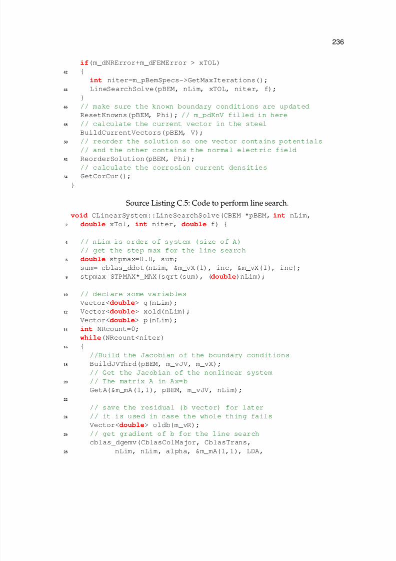
7/18/2019 Riemer PhD 2000


236

if(m_dNRError+m_dFEMError > xTOL)

42

int niter=m_pBemSpecs->GetMaxIterations();

44 LineSearchSolve(pBEM, nLim, xTOL, niter, f);

46 // make sure the known boundary conditions are updated

ResetKnowns(pBEM, Phi); // m_pdKnV filled in here

48 // calculate the current vector in the steel

BuildCurrentVectors(pBEM, V);

50 // reorder the solution so one vector contains potentials

// and the other contains the normal electric field

52 ReorderSolution(pBEM, Phi);

// calculate the corrosion current densities

54 GetCorCur();

Source Listing C.5: Code to perform line search.

void CLinearSystem::LineSearchSolve(CBEM *pBEM, int nLim,

2 double xTol, int niter, double f)

4 // nLim is order of system (size of A)

// get the step max for the line search

6 double stpmax=0.0, sum;

sum= cblas_ddot(nLim, &m_vX(1), inc, &m_vX(1), inc);

8 stpmax=STPMAX*_MAX(sqrt(sum), (double)nLim);

10 // declare some variablesVector<double> g(nLim);

12 Vector<double> xold(nLim);

Vector<double> p(nLim);

14 int NRcount=0;

while(NRcount<niter)

16

//Build the Jacobian of the boundary conditions

18 BuildJVThrd(pBEM, m_vJV, m_vX);

// Get the Jacobian of the nonlinear system

20 // The matrix A in Ax=b

GetA(&m_mA(1,1), pBEM, m_vJV, nLim);

22

// save the residual (b vector) for later

24 // it is used in case the whole thing fails

Vector<double> oldb(m_vR);

26 // get gradient of b for the line search

cblas_dgemv(CblasColMajor, CblasTrans,

28 nLim, nLim, alpha, &m_mA(1,1), LDA,

7/18/2019 Riemer PhD 2000


237

&m_vR(1), inc, beta, &g(1), inc);

30

// save the old unknown variables

32 xold=m_vX;

// and the old f34 fold=f;

// and the residual

36 // this one is updated at each iteration

// and used to check for slow convergence

38 p=m_vR;

// condition the matrix system

40 ConditionSystem(m_mA, p);

N=nLim;

42 NRHS=1;

44

Info=0;char trans=’N’;

46 int strlength=1;

/*****************************************************/

48 // solve Ax=b

#ifdef _DEBUG

50 int rVal;

Vector<Subscript> ipiv(nLim);

52 rVal=LU_factor(m_mA,ipiv, (UPDATEF)UPDATE);

if(rVal==-1)

54

AfxMessageBox("Singular Matrix, Cannot solve.");

56 m_pBemSpecs->SetBemStopFlag();

m_mA.newsize(0,0);

58 return;

60 LU_solve(m_mA,ipiv,p);

#else

62 Vector<Fortran_integer> index(nLim);

DGESV(&N, &NRHS, &m_mA(1,1), &LDA, &index(1),

64 &p(1), &LDB, &Info, (void *)UPDATE);

if(Info>0)

66

AfxMessageBox("Singular Matrix, exiting engine.");68 m_pBemSpecs->SetBemStopFlag();

m_mA.newsize(0,0);

70 return;

72 pBEM->UpdateStatus(89, 4);

#endif

7/18/2019 Riemer PhD 2000


238

74

/*****************************************************/

76 // update the user interface


78 32822, 10);// do the line search

80 // lnsrch tries to find lambda <=1.0 such

// that the norm of the residual is reduced

82 // lambda is the fraction of the full Newton step

lnsrch(pBEM, nLim, m_vR, xold, fold, g, p, m_vX,

84 &f, stpmax, &Info);

86 m_nNR++; // one iteration complete

double test=0.0;

88 // get error

for(ii=0; ii<nLim; ii++)90

if(fabs(m_vR[ii])>test)

92 test=fabs(m_vR[ii]);

94 if(m_pBemSpecs->GetBemStopFlag())

return;

96

// get NRerror

98 if(pBEM->UseAttenuation())

100 int ONE=1;

m_dNRError=cblas_dnrm2(m_nNumNodes, &m_vR(1), ONE);

102 m_dFEMError=cblas_dnrm2(NPZ, &m_vR(m_nNumNodes+1), ONE);




106 32841, (LPARAM)(&m_dFEMError));

108 else

110 int ONE=1;

m_dNRError=cblas_dnrm2(nLim, &m_vR(1), ONE);

112 PostMessage(m_pBemSpecs->GetParentWnd(), WM_COMMAND,32802, (LPARAM)(&m_dNRError));

114

if(test<xTol)

116 break; // break the while loop

118 test=0.0;

7/18/2019 Riemer PhD 2000


239

// check for slow convergence

120 for(ii=0; ii<nLim; ii++)

122 temp=(fabs(m_vX[ii]-xold[ii]))/_MAX(fabs(m_vX[ii]), 1.0);

if(temp>test)124 test=temp;

126 if(test<xTol/10.)

break;

128

C.2.4 Soil Surface On-Potentials

Soil surface on and off-potentials are calculated using equation (3-8). Again,

remote integration is used to actually calculate the integrals necessary to find Φ

at the soil surface. This time, the source points are not on a boundary, so there

are no singular integrals. The results of the integration are again placed in a pair

of matrices that are written to the harddrive.

C.3 Remote Integration

The remote integration module consists of two parts: a client and a server.

The server is a piece of code the actually performs the integration. The client

requests a particular integral or set of integrals to be calculated. Communication

between the client and server is handled through Remote Procedure Calls (RPC).

RPC is a subset of the OpenGroup’s Distributed Computing Environment (DCE).

RPC functions by taking and ordinary function call and passing it over a network

to another computer or to another program on the same computer where the

function is actually executed. The results of the function are then passed back to

the calling program.

7/18/2019 Riemer PhD 2000


240

C.3.1 Interface Definition

To create a callable function that resides on a remote machine, a special piece

of code is created called an interface definition. It contains the definitions of the

data structures that are to be passed to the function in terms of basic data types

such as double, int, or char. It also contains a globally unique identifier to insure

that no-one anywhere else in the world has made a definition the same as this

one. Finally the code contains the definitions of the functions that are to be called.

Each parameter passed to the function contains a label as to whether the param-

eter is an input, output or both. This is done to reduce the amount of data that

must be transported across the network when the function is called and when it

returns. The interface definition for pipeline model integration subroutines is

Source Listing C.6: Interface definition for remote integration module.

[ uuid

2 (e4e1a780-df39-11d3-80c0-00c04f6b9a47),

version(4.0),

4 pointer_default(unique)

] interface CPInt6

typedef struct _NODE

8 double x;

double y;

10 double z;

NODE;

12

typedef struct _ELEMENT

14 NODE theNodes[9];

long nEletype;

16 ELEMENT;

18

typedef struct _INTPARAMETERS

20 double dRelErr;

double dLedgePos;

22 long nUseLedgePos;

long nIntScheme; //pos means singular

7/18/2019 Riemer PhD 2000


241

24 long nUseHighSpeed;

INTPARAMETERS;

26

typedef struct _INTDATA

28 ELEMENT theElement;NODE theColnode;

30 INTPARAMETERS thePrams;

INTDATA;

32

typedef struct _RESULTS

34 double theResults[18];

RESULTS;

36

typedef struct _DOMAINRESULTS

38 double theResults[3][18];

DOMAINRESULTS;40

DOMAINRESULTS IntegrateDomainPoints(

42 [in] handle_t hBind,

[in] INTDATA data);

44

RESULTS IntegrateElement(

46 [in] handle_t Binding,

[in] INTDATA theData);

48

long GetNumProcessors(

50 [in] handle_t Binding);

;

There is an extra function added to tell the client program how many proces-

sors are available to do calculations. Then the client program can create as many

parallel called threads as there are processors.

The above code is written in what is called Interface Definition Language

(IDL). It is also used by another remote procedure technique called CORBA. A

CORBA interface has also been written for the model code.

7/18/2019 Riemer PhD 2000


242

C.3.2 Data Marshaling

DCE RPC has been built with cross-platform capability in mind. Cross-platform

means the client and server do not have to be on the same operating system or

hardware type. Therefore, a standard must be created for the transport of data

between the client and server so that when the data is reassembled, it is identical

to the original that was sent. If the client has Little Endian hardware (least sig-

nificant byte first) and the server is a Big Endian machine (most significant byte

first), there must be mechanisms to correctly assemble the data. This is where

data marshaling in needed. Data marshaling takes the data being sent from one

machine to another and translates it into a standard byte stream format. Then the

bytes can be reasembled into the original data using the appropriate standard for

the hardware of the machine.

The code to marshal the data is created by an IDL compiler. The compiler

reads the IDL file and creates a client stub that exposes the functions to the client

program, marshals the data and sends the function call and data to the remote

machine. The compiler also creates the server stub that calls the function on the

remote machine. The server stub also takes the data sent to it and formats it into

the proper variables for the server function call.

Transport across the network is handled by a standard packet technique such

TCP or UDP which are protocols in the TCP/IP family of network protocols. In

the case of this code, only TCP is used.

7/18/2019 Riemer PhD 2000


243

C.3.3 Server Side

The server portion of the code is a stand-alone program that runs on every

computer that will be used in the parallel computation. Since it would be very

inconvenient to start each program manually, the code is written as a system ser-

vice and network listener. That way, the code is always ready to do a calculation

but does not use any computer time when not in use.

The code is loaded into memory whenever the computer boots and does not

shut down again until the computer is shutdown. It also listens on a TCP port for

requests to calculate an integral. Since the computer can possibly receive requests

from several computers simultaneously, or the server computer may have more

than one CPU, the code is multi-threaded. This means there can be more than

one calculation running at the same time.

When the code is loaded into memory, a startup routine is called which then

blocks on a listen command until the computer is shutdown. The sequence of

task at startup is

1. Select a protocol for network transport. This is the language used to com-

municate data between the client program and the server program.

2. Register the existence of the listener with the RPC endpoint mapper.

3. Listen for calls to calculate integrals.

The first task is accomplished by the code shown is listing C.7.

Source Listing C.7: Selection of communication protocol for remote procedurecall.

// use tcp/ip protocol ncacn

2 status=RpcServerUseProtseqEp(

7/18/2019 Riemer PhD 2000


244

(unsigned char *)"ncacn_ip_tcp", // protocol

4 cMaxCalls, // max simultaneous threads

(unsigned char *)"3643", // port to listen on

6 pszSecurity); // security requirements

if(status)8 goto cleanup;

// use non network protocol ncalrpc

10 // this listener only works when the client is

// located on the same machine

12 status=RpcServerUseProtseqEp(

(unsigned char *)"ncalrpc", //local only

14 cMaxCalls, // max simultaneous threads

(unsigned char *)"cp3dint400", //endpoint name

16 pszSecurity); // security requirements

if(status)

18

goto cleanup;// let the operating system known we are still alive

20 ReportStatusToSCMgr(

SERVICE_START_PENDING, // service state

22 NO_ERROR, // exit code

3000); // wait hint

Then the listener is registered with the RPC endpoint mapper with calls to the

RPC service as shown in listing C.8.

Source Listing C.8: Registration of RPC server.

// interface to register

2 status = RpcServerRegisterIf(CPInt_v4_0_s_ifspec,

NULL, // MgrTypeUuid

4 NULL);

6 // get the binding vector handle

status = RpcServerInqBindings(&pBindingVector);

8

if (status)

10 goto cleanup;

// register the endpoints

12 status = RpcEpRegister(CPInt_v4_0_s_ifspec,

pBindingVector,

14 NULL,

NULL);

7/18/2019 Riemer PhD 2000


245

Finally, the code tells the operating system that all is well and the program is

listening for requests as shown in listing C.9. There is one more step in the code,

setting the priority class for the service in line 6 of listing C.9. It is set to idle sothat the code does not interfere with other processes the user of the machine may

be using. In essence, the code will only use what would otherwise be unused

CPU cycles.

Source Listing C.9: Code to start listening for integration calculation requests.

ReportStatusToSCMgr(

2 SERVICE_RUNNING, // service state

NO_ERROR, // exit code

4 0);

// set the priority

6 SetPriorityClass(GetCurrentProcess(),

IDLE_PRIORITY_CLASS);

8 //start listening for calls

status = RpcServerListen(cMinCalls,

10 cMaxCalls,

fDontWait );

The code blocks on the call RpcServerListen() until shutdown. In order

for the code to respond to requests, extra threads are created that actually run the

functions.

C.3.4 Client Side

The client side of the remote integration procedure is implemented within

the calculation engine of the main program. It consists of two classes that work

together to complete all of the integration with the least amount of local CPU

effort. The first of the two classes (CDomainData) will have only one instance

during the life of the integration process, while there will be one instance of the

7/18/2019 Riemer PhD 2000


246

second class (CRpcIntegrate) for every CPU on every machine involved with

the integration.

The integration process starts by creating a list of “jobs” to be done. Each jobconsists of either 12 or 18 integrals to be completed depending on if the element

over which the integrals are to be computed are triangles or rectangles. Each

job is stored in a last-in-first-out (LIFO) stack saved to disk. This task is carried

out by the first class described above (CDomainData). Once the data has been

sorted and placed as discrete jobs in a stack, the main program spawns off a

new thread for each CPU. Each thread creates an instance of CRpcIntegrate

with the parameters of the machine name that the thread should send integration

requests to and a handle to the CDomainData object.

Source Listing C.10: Code to spin off integration threads for each CPU on eachmachine.

void CLinearSystem::AssembleMatrices(CBEM *pBEM)

2 ...

// start a thread for each machine

4 POSITION pos=pDB->GetHeadPos();

while(pos!=NULL)

6

CComputerRecord *pRec=pDB->GetNext(pos);

8 CString str=pRec->GetName();

10 // find number of CPUs on this system

int nCPUs=GetNumCPUs( str);

12 // start a new thread with this name

for(int jj=0; jj<nCPUs; jj++)

14

pData=new INTSTARTDATA;

16 pData->pData=m_pBemThreadData;pData->bIsGroundCalc=FALSE;

18 pData->bUseLocalRpc=FALSE;

pData->strName=str;

20 if(m_pBemSpecs->GetConvTolSetting()==0)

pData->bUseHighSpeed=TRUE;

22 else

7/18/2019 Riemer PhD 2000


247

pData->bUseHighSpeed=FALSE;

24 pData->bWantSing=FALSE;

DWORD dwThreadID;

26 pThread=CreateThread(NULL, 0,

(LPTHREAD_START_ROUTINE)IntegrationControl,28 pData, CREATE_SUSPENDED, &dwThreadID);

// set thread priority high

30 SetThreadPriority(pThread, THREAD_PRIORITY_ABOVE_NORMAL);

ResumeThread(pThread);

32 pThreadList.AddTail(pThread);

34

BOOL done=FALSE;

36 // now monitor

unsigned int count=0;

38

while(!done)

40 count++;

Sleep(250); // sleep a quarter second

42 BOOL bStillAlive=FALSE;

DWORD bStatus;

44 POSITION pos=pThreadList.GetHeadPosition();

while(pos!=NULL)

46

HANDLE pT=pThreadList.GetNext(pos);

48 GetExitCodeThread(pT , &bStatus);

if(bStatus==STILL_ACTIVE )

50 bStillAlive=TRUE;

52 if(!bStillAlive)

done=TRUE;

54

Listing C.10 shows the code that creates the threads that send integration jobs

to remote machines. Line 26 contains the code that starts a new thread in a sus-

pended state. This allows the main thread to set the thread priority before its

execution is resumed. The high priority level given to the service threads may

seem as though they should cause poor execution of other tasks in the program.

7/18/2019 Riemer PhD 2000


248

That is not true, however, because most the the time the thread is blocked waiting

for a remote procedure call to complete (see line 96 of listing C.11).

The CRpcIntegrate object starts by making a connection to the machine itis to talk to. It then goes into a loop consisting of three tasks: 1) get a job from

CDomainData, 2) make a remote procedure call, 3) If the call succeeds, write the

results to the matrices; otherwise write the job to the error stack for some other

thread to complete.

Source Listing C.11: Client code to make a remote procedure call.

int CRpcIntegrate::Integrate()

2

unsigned long ulCode;

4 unsigned char * pszStrBinding = NULL;

unsigned char * pszOptions = NULL;

6 unsigned char * pszUuid = NULL;

RPC_BINDING_HANDLE hCP3D;

8 RPC_STATUS status;

int fContinue=1;

10 RpcTryExcept

EnterCriticalSection(&CRPCIntThread::m_csDataLock);

12

if(!m_bUseLocalRPC)14

status=RpcStringBindingCompose( pszUuid,

16 (unsigned char *) "ncacn_ip_tcp",

(unsigned char *)m_strMachineName,

18 (unsigned char *) "3643",

pszOptions,

20 &pszStrBinding);

22 else

24 status=RpcStringBindingCompose( pszUuid,

(unsigned char *) "ncalrpc",

26 NULL,

(unsigned char *) "cp3dint400",

28 pszOptions,

&pszStrBinding);

30

7/18/2019 Riemer PhD 2000


249

32 LeaveCriticalSection(&CRPCIntThread::m_csDataLock);

34 RpcExcept(1)

ulCode = RpcExceptionCode();

36 fContinue = 0;

38 RpcEndExcept

if(status!=RPC_S_OK)

40 return -1;

42 // get the binding

RpcTryExcept

44 EnterCriticalSection(&CRPCIntThread::m_csDataLock);

46 status = RpcBindingFromStringBinding(pszStrBinding,

&hCP3D);48

LeaveCriticalSection(&CRPCIntThread::m_csDataLock);

50

RpcExcept(1)

52 ulCode = RpcExceptionCode();

fContinue = 0;

54

RpcEndExcept

56 if(status!=RPC_S_OK)

58 RpcBindingFree(&hCP3D);

return -1;

60

//else we are good to go with a live connection

62

BOOL bDone=FALSE;

64 BOOL bGotSing;

INTDATA intData; // data to be sent

66 JOBSTACK job; // job to do

CBemSpecs *pSpecs;

68 CSoilZoneDataBase *pSZDB;

EnterCriticalSection(&CRPCIntThread::m_csFileLock);

70 pSpecs=m_pThreadData->GetBemSpecs();

72 pSZDB=pSpecs->GetSoilZoneDB();

74 LeaveCriticalSection(&CRPCIntThread::m_csFileLock);

CSoilZoneRecord *pRec;

76 int ii;

7/18/2019 Riemer PhD 2000


250

while(!bDone)

78


80

if(!m_pThreadData->GetJob(job, &bGotSing,82 m_bWantSing))

84 LeaveCriticalSection(

&CRPCIntThread::m_csDataLock);

86 bDone=TRUE;

break;

88

90 LeaveCriticalSection(&CRPCIntThread::m_csDataLock);

BOOL bResultsGood=TRUE;

92

RESULTS theResults; // the returned data// make the RPC call

94 RpcTryExcept

96 theResults = IntegrateElement(hCP3D, intData);

98 RpcExcept(1)

ulCode = RpcExceptionCode();

100 fContinue = 0;

bResultsGood=FALSE;

102 HandleRPCError(pSpecs, job, intData, hCP3D);


104

// check for quit message

106 if(m_pThreadData->ShouldStopCalc())

108 LeaveCriticalSection(

&CRPCIntThread::m_csDataLock);

110 return 0;

112


114

RpcEndExcept116 if(bResultsGood)

118 EnterCriticalSection(&CRPCIntThread::m_csDataLock);

120 m_pThreadData->WriteFinishedWork(job,

&theResults);

7/18/2019 Riemer PhD 2000


251

122


124

126 RpcBindingFree(&hCP3D);

128 return 0;

A byproduct of this technique is that it implicitly balances the computational

load over a heterogeneous network of workstations. The balancing is done be-

cause the technique supplies a relatively small packet of information that can be

completed in about 1 second on a Pentium III 500 mhz CPU.

7/18/2019 Riemer PhD 2000


REFERENCES

1. Gas Facts - Distribution and Transmission Miles of Pipeline,Technical report, American Gas Association (1999).Http://www.aga.org/StatsStudies/GasFacts/2131.html.

2. NTSB, Pipline Accident Summary Report: Pipeline Rupture, Liquid Butane Re-lease, and Fire, Lively, Texas August 24 1996, Technical report, National Trans-portation Safety Board, Washington, D.C. (1998).

3. J. Morgan, Cathodic Protection, 2nd edition (Houston, TX: NACE, Interna-tional, 1993).

4. M. L. Wald, “Conglomerate, Accused of Allowing Spills to Cut Costs, Is

Fined $30 Million,” New York Times, (January, 14 2000).

5. Gorton, “Pipeline Safety Improvement Act of 2000,” in Congressional Record,102nd Congress, 2nd Session (Government Printing Office, 2000) S8225.

6. McCain, “AMENDMENT NO. 4130 to Pipeline Safety Improvement Act of 2000,” in Congressional Record, 102nd Congress, 2nd Session (GovenmentPrinting Office, 2000) S8231.

7. J. Wagner, Cathodic Protection Design I , NACE, International, Houston, TX(1994).

8. C. Kasper, “The Theory of the Potential and the Technical Practice of Elec-trodeposition: IV. The Flow between and to Circular Cylinders.” Transactionsof the Electrochemical Society, 78 (1940) 147–161.

9. J. O. M. Bockris and A. K. N. Reddy, Modern Electrochemistry: Ionics, vol-ume 1, 2nd edition (New York: Plenum Press, 1998).

10. J. O. M. Bockris and A. K. N. Reddy, Modern Electrochemistry: Electrodics,volume 2, 2nd edition (New York: Plenum Pub, 2000).

11. A. J. Bard and L. R. Faulkner, Electrochemical Methods: Fundamentals and Ap- plications (New York: Wiley, 1980).

12. J. S. Newman, Electrochemical Engineering, 2nd edition (Englewood Cliffs,New Jersey: Prentice-Hall, 1991).

13. J. O. Bockris, D. Drazic, and A. R. Despic, “The Electrode Kinetics of theDeposition and Dissolution of Iron,” Electrochimica Acta, 4 (1961) 325–361.

252

7/18/2019 Riemer PhD 2000


253

14. M. E. Orazem and J. M. Esteban, Phase II Final Report: A Three Dimensional Model for the Cathodic Protection of an Underground PIpeline, Technical report,University of Florida (1994).

15. G. Jerkiewicz, “Hydrogen Sorption At/In Electrode,” Progress in Surface Sci-ence, 57 (1998) 137–186.

16. M. de Chialvo and A. Chialvo, “The Tafel-Heyrovsky route in the kineticmechanism of the hydrogen evolution reaction,” Electrochemistry Communi-cations, 1 (1999) 379–382.

17. M. de Chialvo and A. Chialvo, “Existence of two sets of kinetic parametersin the correlation of the hydrogen electrode reaction,” Journal of the Electro-chemical Society, 147 (2000) 1619–1622.

18. A. Lasia and D. Gregoire, “General Model of Electrochemical Hydrogen Ab-

sorption Into Metals,” Journal of the Electrochemical Society, 142 (1995) 3393–3399.

19. L. J. Bai, “Behavior of a Hydride Phase Formed in the Hydrogen EvolutionReaction at a Rotating Pt Electrode - Analysis of Potential Relaxation Tran-sients from a Kinetic Approach,” Journal of Electroanalytical Chemistry, 355(1993) 37–55.

20. K. Nisancioglu, “Predicting the Time Dependence of Polarization on Ca-thodically Protected Steel in Seawater,” Corrosion, 43 (1987) 100–111.

21. K. Nisancioglu, P. O. Gartland, T. Dahl, and E. Sander, “Role of Surface

Structure and Flow Rate on the Polarization of Cathodically Protected Steelin Seawater,” Corrosion, 43 (1987) 710–718.

22. P. Nisancioglu, K. Gartland, “Current Distribution with Dynamic BoundaryConditions,” in I. Chem. Symposium Series No. 112: Conference on Electrochem-ical Engineering (Loughborough: Loughborough University of Technology,1989) .

23. J. F. Yan, S. N. R. Pakalapati, T. V. Nguyen, R. E. White, and R. B. Griffin,“Mathematical Modeling of Cathodic Protection Using the Boundary Ele-ment Method with a Nonlinear Polarization Curve,” Journal of the Electro-

chemical Society, 139 (1992) 1932–1936.24. K. Kennelley, L. Bone, and M. Orazem, “Current and Potential Distribution

on a Coated Pipeline with Holidays Part I - Model and Experimental Verifi-cation.” Corrosion, 49 (1993) 199–210.

25. D. A. Jones, Principles and Prevention of Corrosion (Upper Saddle River, NJ:Prentice Hall, 1996).

7/18/2019 Riemer PhD 2000


254

26. A. Korzhenko, M. Tabellout, and J. Emery, “Dielectric Relaxation Propertiesof the Polymer Coating During its Exposition to Water,” Materials Chemistryand Physics, 65 (2000) 253–260.

27. C. Corfias, N. Pebere, and C. Lacabanne, “Characterization of a Thin Pro-tective Coating on Galvanized Steel by Electrochemical Impedance Spec-troscopy and a Thermostimulated Current Method,” Corrosion Science, 41(1999) 1539–1555.

28. I. Margarit and O. Mattos, “About Coatings and Cathodic Protection: Pos-sibilities of Impedance as Monitoring Technique,” in Electrochemical Methodsin Corrosion Research VI, Parts 1 and 2 (Zurich-Eutikon: Transtec Publications,1998) 279–292.

29. I. Thompson and D. Campbell, “Interpreting Nyquist Responses From De-fective Coatings on Steel Substrates,” Corrosion Science, 36 (1994) 187–198.

30. F. Bellucci and L. Nicodemo, “Water Transport in Organic Coatings,” Corro-sion, 49 (1993) 235–247.

31. D. Riemer and M. Orazem, “Development of Mathematical Models forCathodic Protection of Multiple Pipelines in a Right of Way,” in Proceed-ings of the 1998 International Gas Research Conference, Gas Research Institute(Chicago: GRI, 1998) 117. Paper TSO-19.

32. D. Riemer and M. Orazem, “Cathodic Protection of Multiple Pipelines withCoating Holidays,” in Procedings of the NACE99 Topical Research Symposium:Cathodic Protection: Modeling and Experiment, M. E. Orazem, editor, NACE(Houston, TX: NACE International, 1999) 65–81.

33. M. Orazem, J. Esteban, K. Kenelley, and R. Degerstedt, “Mathematical Mod-els for Cathodic Protection of an Underground Pipeline with Coating Holi-days: Part 1 - Theoretical Development,” Corrosion, 53 (1997) 264–272.

34. D. Diakow, G. Van Boven, and M. Wilmott, “Polarization Under DisbondedCoatings: Conventional and Pulsed Cathodic Protection Compared,” Mate-rials Performance, 37 (1998) 17–23.

35. T. R. Jack, “External Corrosion of Line Pipe - a Summary of Research Activ-

ities,” Materials Performance, 35 (1996) 18–24.36. J. A. Beavers and N. G. Thompson, “Corrosion Beneath Disbonded

Pipeline,” Materials Performance, 36 (1997) 13–19.

37. R. Aris, Vectors, Tensors and the Basic Equations of Fluid Mechanics (New York:Dover Publications, Inc., 1962).

7/18/2019 Riemer PhD 2000


255

38. H. M. Deitel and P. J. Deitel, C++: How to Program, 3rd edition (Upper SadleRiver, NJ: Prentice Hall, 2000).

39. B. Eckel, Thinking in C++, Volume 1, 2nd edition (Upper Saddle River, NJ:

Prentice Hall, 2000).40. A. W. Peabody, Control of Pipeline Corrosion (Houston, TX: NACE, 1978).

41. K. E. Jeffers, Electrochemical Impedance Spectroscopy for the Characterization of Corrosion and Cathodic Protection of Buried Pipelines, Master’s thesis, Univer-sity of Florida, Gainesville, Florida (1999).

42. D. R. Baker, M. W. Verbrugge, and J. Newman, “A Transformation for theTreatment of Diffusion and Migration. Application to Stationary Disk andHemispherical Electrodes,” Journal of Electroanalytic Chemistry, 314 (1991)23–44.

43. D. R. Baker, “Reducing Nonlinear Systems of Transport Equations toLaplace’s Equation,” SIAM Journal of Applied Math, 53 (1993) 419–439.

44. B. Pillay and J. Newman, “Modeling Diffusion and Migration in Dilute Elec-trochemical Systems Using the Quasipotential Transformation,” Journal of the Electrochemical Society, 140 (1993) 414–420.

45. M. W. Verbrugge, D. R. Baker, and J. Newman, “Dependent-Variable Trans-formation for the Treatment of Diffusion, Migration, and Homogeneous Re-actions,” Journal of the Electrochemical Society, 140 (1993) 2530.

46. K. Allahar and M. Orazem, “Modeling Disbonded Coatings using the

Quasipotential Transformation,” in Passivity and Localized Corrosion, R. G.Kelly, B. MacDougall, M. Seo, and H. Takahashi, editors, volume PV-99-27(Pennington, N.J.: Electrochemical Society, Inc., 1999) 609.

47. H. S. Carslaw and J. C. Jaeger, Conduction of Heat in Solids (New York: OxfordUniversity Press, 1959).

48. H. F. Moulton, “Current Flow in Rectangular Conductors,” Proceedings of theLondon Mathematical Society, ser. 2 (1905) 104–110.

49. F. Bowman, Introduction to Elliptic Functions with Applications (New York: John Wiley and Sons, 1953).

50. M. E. Orazem and J. Newman, “Primary Current Distribution and Resis-tance of a Slotted-Electrode Cell,” Journal of the Electrochemical Society, 131(1984) 2857–2861.

51. M. E. Orazem, “Calculation of the Electrical Resistance of a Compact Ten-sion Specimen for Crack-Propagation Measurements,” Journal of the Electro-chemical Society, 132 (1985) 2071–2076.

7/18/2019 Riemer PhD 2000


256

52. M. E. Orazem and W. Ruch, “An Improved Analysis of the Potential DropMethod for Measuring Crack Lengths in Compact Tension Specimens,” In-ternational Journal of Fracture, 31 (1986) 245–258.

53. C. B. Diem, B. Newman, and M. E. Orazem, “The Influence of Small Machin-ing Errors on the Primary Current Distribution at a Recessed Electrode,” Journal of the Electrochemical Society, 135 (1988) 2524–2530.

54. C. A. Brebbia and J. Dominguez, “Boundary Element Methods for PotentialProblems,” Applied Mathematical Modelling, 1 (1977) 371–378.

55. S. Aoki, K. Kishimoto, and M. Sakata, “Boundary Element Analysis of Gal-vanic Corrosion,” in Boundary Elements VII , C. A. Brebbia and G. Maier, edi-tors, volume 1 (Berlin: Springer-Verlag, 1985) 73–83.

56. J. Telles, L. Wrobel, W. Mansur, and J. Azevedo, “Boundary Elements for

Cathodic Protection Problems,” in Boundary Elements VII , B. C. M. G, editor,volume 1 (Springer-Verlag, 1985) 63–71.

57. N. Zamani and J. Chuang, “Optimal-Control of Current in a Cathodic Pro-tection System - A Numerical Investigation,” Optimal Control Applications &

Methods, 8 (1987) 339–350.

58. F. Brichau and J. Deconinck, “Numerical model for cathodic protection of buried pipes,” Corrosion, 50 (1994) 39–49.

59. F. Brichau, J. Deconinck, and T. Driesens, “Modeling of Underground Ca-thodic Protection Stray Currents,” Corrosion, 52 (1996) 480–488.

60. S. Aoki and K. Amaya, “Optimization of Cathodic Protection SYstem byBEM,” Engineering Analysis with Boundary ELements, 19 (1997) 147–156.

61. S. Aoki, K. Amaya, and M. Miyasaka, “Boundary Element Analysis of Ca-thodic Protection for Complicated Structures,” in Procedings of the NACE99Topical Research Symposium: Cathodic Protection: Modeling and Experiment,M. E. Orazem, editor, NACE (Houston, TX: NACE International, 1999) 45–65.

62. C. Brebbia and J. Dominguez, Boundary Elements: An Introductory Course(Avon, Great Britain: McGraw-Hill, The Bath Press, 1989).

63. C. A. Brebbia, J. C. F. Telles, and L. C. Wrobel, Boundary Element Techniques(Springer-Verlag, 1984).

64. F. Hartmann, C. Katz, and B. Protopsaltis, “Boundary Elements and Sym-metry,” INGENIEUR ARCHIV , 55 (1985) 440–449.

7/18/2019 Riemer PhD 2000


257

65. L. Gray and G. Paulino, “Symetric Galerkin Boundary Integral Formulationfor Interface and Multi-zone Problems,” International Journal for Numerical

Methods in Engineering, 40 (1997) 3085–3101.

66. I. Stakgold, Greens Functions and Boundary Value Problems (New York: JohnWiley & Sons, 1979).

67. D. S. Burnett, Finite Element Analysis (Reading Mass: Addison-Wesley, 1987).

68. J. W. Gibbs, The Scientific Papers Vol. II (New York: Dover Pub. Inc., 1961).

69. J. C. F. Telles and F. A. D. Paula, “Boundary Elements with Equilibrium Sat-isfaction - a Consistent Formulation for Potential and Elastostatic Analysis,”International Journal of Numerical Methods in Engineering, 32 (1991) 609–621.

70. J. Trevelyan and H. Hack, “Analysis of stray current corrosion problemsusing the boundary element method,” in Boundary Element Technology IX (Boston: Computational Mechanics Publications, 1994) 347–356.

71. S. Aoki and K. Kishimoto, “Application of BEM to Galvanic Corrosion andCathodic Protection,” in Topics in Boundary Element Research: Electrical En-

gineering Applications, C. Brebbia, editor, volume 7 (Heidelberg, Germany:Springer-Verlag, 1990) 103–120.

72. W. Press, S. A. Teukolsky, W. T. Vetterling, and B. P. Flannery, NumericalRecipes in C: the Art of Scientific Computing, 2nd edition (New York: Cam-

bridge University Press, 1992).

73. S. Burton, K. E. Garbow, J. J. Hillstrom, and Others, “Modified PowellMethod with Analytic Jacobian,” Software source code hybrdj.f (1980). Ar-gonne National Laboratory. minpack project. www.netlib.org/minpack.

74. T. J. Hughes, The Finite Element Method: Linear Static and Dynamic Finite Ele-ment Analysis (Englewood Cliffs, New Jersey: Prentice-Hall, 1987).

75. J. R. Shewchuk, “Triangle: Engineering a 2D Quality Mesh Generator andDelaunay Triangulator,” in First Workshop on Applied Computational Geometry(Philidelphia: ACM, 1996) 124–133.

76. J. Ruppert, “A Delaunay Refinement Algorithm for Quality 2-Dimensional

Mesh Generation,” Journal of Algorithms, 18 (1995) 548–585.77. J. R. Shewchuck, “Triangle: Engineering a 2D Quality Mesh Generator and

Delaunay Triangulator,” in Applied Computational Geometry: Towards Geomet-ric Engineering, M. C. Lin and D. Manocha, editors, volume 1148 of LectureNotes in Computer Science (Philadelphia, PA: Springer-Verlag, 1996) 203–222,203–222. From the First ACM Workshop on Applied Computational Geom-etry.

http://www.netlib.org/minpack

7/18/2019 Riemer PhD 2000


258

78. J. R. Shewchuck, “Triangle.c: A Two-Dimensional Qual-ity Mesh Generator and Delaunay Triangulator,” SourceCode (1996). www.netlib.org/voroni/triangle.shar andwww.cs.cmu.edu/

∼quake/triangle.html.

79. G. Beer and J. Meek, “Inifinte Domain Elements,” International Journal of Nu-merical Methods in Engineering, 17 (1981) 43–52.

80. M. Aliabadi and W. Hall, “Taylor Expansions for Singular Kernals in theBoundary Element Method,” International Journal of Numerical Methods in En-

gineering, 21 (185) 2221–2236.

81. M. Cristescu and G. Loubignac, “Gaussian Quardrature Formulas for Func-tions with Singularities in 1/r over Triangles and Quadrangles,” in Bound-ary elements VII : proceedings of the 7th international conference, Villa Olmo, LakeComo, Italy, September 1985, C. Brebbia and G. Maier, editors (New York:

Springer-Verlag, 1985) 375–390.

82. H. Pina, J. Fernandes, and C. Brebbia, “Some Numerical Integration Formu-lae over Triangles and Squares with a 1/r Singularity,” Applied Mathematical

Modelling, 5 (1981) 209–211.

83. M. Guiggiani and C. Paolo, “Direct Computation of Cauchy Principal ValueIntegrals in Advanced Boundary Elements,” Intenational Journal for Numeri-cal Methods in Engineering, 24 (1987) 1711–1720.

84. M. Guiggiani and A. Gigante, “A General Algorithm for MultidimensionalCauchy Principal Value Integrals in the Boundary Element Method,” Journalof Applied Mechanics, 57 (1990) 906–915.

85. D. Rosen and D. Cormack, “Singular and Near Singular Integrals in theBEM: A Global Approach,” Society for Industrial and Applied Mathematics:

Journal of Applied Mathematics, 53 (1993) 340–357.

86. O. Almeida Pereira and P. Parreira, “Direct Evaluation of Cauchy Prin-cipal Value Integrals in Boundary Elements for Infinte and Semi-infiniteThree-Dimensional Domains,” Engineering Analysis with Boundary Elements,13 (1994) 313–320.

87. W. Sun and N. Zamani, “An Adaptive h-r Boundary Element Algorithm forthe Laplace Equation,” Intenational Journal for Numerical Methods in Engineer-ing, 33 (1992) 537–552.

88. N. Kamiya and M. Koide, “Adaptive Boundary Element for Multiple Subre-qions,” Computational Mechanics, 12 (1993) 69–80.

http://www.cs.cmu.edu/~quake/triangle.html

http://www.netlib.org/voroni/triangle.shar

7/18/2019 Riemer PhD 2000


259

89. A. Karafiat, “Adaptive Integration Techniques for Almost Singular Func-tions in the Boundary Element Method,” Computers Mathematics with Appli-cations, 32 (1996) 11–30.

90. M. Guiggiana, G. Krishnasamy, T. J. Rudolphi, and F. J. Rizzo, “A GeneralAlgorithm for the Numerical Solution of Hypersingular Boundary IntegralEquations,” Journal of Applied Mechanics, 59 (1992) 604–614.

91. R. Cools, D. Laurie, and L. Pluym, A User Manual for Cubpack++ version 1.1,K.U. Leuven, Belgium (1997).

92. I. Visual Numerics, “IMSL Subroutines,” Software Library (2000).

93. E. De Donker and I. Robinson, “Algorithm for Automatic Integration over aTriangle using Non-linear Extrapolation,” ACM-Tran.s Math. Soft., 10 (1984)1–16.

94. E. De Donker and I. Robinson, “Triex: Integration over a Triangle usingNon-linear Extrapolation,” ACM-Tran.s Math. Soft, 10 (1984) 17–22. Sourcecode available from http://www.netlib.org/toms/612, May 10, 1999.

95. R. Cools, D. Laurie, and L. Pluym, “Algorithm 764: Cubpack++: A C++Package for Automatic Two-Dimensional Cubature,” ACM Transactions on

Mathematical Software, 23 (1997) 1–15.

96. “LAPACK – Linear Algebra PACKage,” Source Code (2000).www.netlib.org/lapack accessed November 2, 2000 - version 3.0 avail-able.

97. “BLAS - BLAS (Basic Linear Algebra Subprograms),” Source Code (2000).www.netlib.org/blas accessed November 2, 2000.

98. “Intel R Math Kernal Library,” Libaries (archive) (2000). devel-oper.intel.com/vtune/perflibst/mkl Accessed November 2, 2000.

99. J. Newman, “Resistance for Flow of Current to a Rotating Disk,” Journal of the Electrochemical Society, 113 (1966) 501–502.

100. N. W. Cluts, Programming the Windows 95 User Interface (Microsoft Press,1996).

101. M. Corporation, editor, The Windows Interface: Guidelines for Software Design(Microsoft Press, 1995).

102. “OpenGL 3-D Rendering Software v. 1.2,” Software Library, Silicon Graphics(1999). www.opengl.org.

103. R. Hall and D. Forsyth, Interactive 3D Graphics in Windows (New York:Springer-Verlag, 1995).

http://www.opengl.org/

http://developer.intel.com/vtune/perflibst/mkl

http://developer.intel.com/vtune/perflibst/mkl

http://www.netlib.org/blas

http://www.netlib.org/lapack

http://www.netlib.org/toms/612

7/18/2019 Riemer PhD 2000


260

104. C. in Perspective, “Joey Toolkit, vers. 5.6,” Software (1998). Windows95/98/NT, 10MB compressed file.

105. R. S. Wright and M. Sweet, OpenGL SuperBible, 2nd edition (Waite Group,

1999).106. M. Woo, J. Neider, T. David, D. Shriner, and T. Davis, OpenGL(r) 1.2 Program-

ming Guide, Third Edition: The Official Guide to Learning OpenGL, Version 1.2,3rd edition (Addison-Wesley, 1999).

107. A. J. Davies, “Parallel Implementations of the Boundary Element Method,”Computers Math. Applic, 31 (1996) 33–40.

108. E. De Santiago and H. Kincho, “A Distributed Finite Element Method forSolving the Incompressible Navier-Stokes Equations,” International Journal

for Numerical Methods in Engineering, 39 (1996) 4243–4258.

109. K. J. Kennelley, L. Bone, and M. E. Orazem, “Current and Potential Dis-tribution on a Coated Pipeline with Holidays: 1. Model and ExperimentalVerification,” Corrosion, 49 (1993) 199–210.

110. M. E. Orazem, K. J. Kennelley, and L. Bone, “Current and Potential Distri- bution on a Coated Pipeline with Holidays: 2. A Comparison of the Effectsof Discrete and Distributed Holidays,” Corrosion, 49 (1993) 211–219.

111. M. E. Orazem, J. M. Esteban, K. J. Kennelley, and R. M. Degerstedt, “Math-ematical Models for Cathodic Protection of an Underground Pipeline withCoating Holidays: 2. Case Studies of Parallel Anode CP Systems,” Corrosion,

53 (1997) 427–436.

112. R. M. Degerstedt, K. J. Kennelley, M. E. Orazem, and J. M. Esteban, “Tra-ditional Cathodic Protection Design Methods for Coated Pipelines and theNecessity of Computer Modeling,” Materials Performance, 35 (1996) 16–20.

113. S. P. Turnipseed and G. Nekoksa, “Potential Measurement on Cathodi-cally Protected Structures Using an Integrated Salt Bridge and Steel RingCoupon,” Materials Performance, 35 (1996) 21–25.

114. C. D. Stears, O. C. Moghissi, and L. Bone, “Use of Coupons to Monitor Ca-thodic Protection of an Underground Pipeline,” Materials Performance, 37

(1998) 23–31.

115. K. M. Lawson and N. G. Thompson, “The Use of Coupons for Monitoringthe Cathodic Protection of Buried Structures,” in Corrosion 98 (Houston, TX:Nace International, 1998) Paper No. 672.

7/18/2019 Riemer PhD 2000


261

116. K. J. Kennelley, M. E. Orazem, J. M. Esteban, and R. M. Degerstedt, “Full-Scale Laboratory Evaluation of Parallel Anode CP Systems for CoatedPipelines with Comparison to 2 and 3-D Models,” in Proceedings of Corro-sion/95 (Houston, Texas: National Association of Corrosion Engineers, 1995)

Paper 528.

117. P. A. Collins, K. C. Garrity, C. J. Pieper, R. P. Siegel, P. J. Smith, and G. E.Tesch, editors, Aboveground Storage Tanks: Current Issues - Design, Operations,

Maintenance, Inspection and the Environment (Houston, TX: NACE, 1992).

118. L. Koszewski, “Retrofitting Asphalt Storage Tanks with an Improved Ca-thodic Protection System,” Materials Performance, 38 (1999) 20–24.

119. M. Abramowitz and I. A. Stegun, Handbook of Mathematical Functions (NewYork, New York: Dover Publications, 1972).

120. D. H. Kroon, “Cathodic Protection of Aboveground Storage Tank Bottoms,” Materials Performance, 33 (1994) 26–30.

121. W. H. Smyrl and J. Newman, “Detection of Nonuniform Current Distribu-tion on a Disk Electrode,” Journal of the Electrochemical Society, 119 (1972)208–212.

122. J. Newman, “Current Distribution on a Rotating Disk below the LimitingCurrent,” Journal of the Electrochemical Society, 113 (1966) 1235–1241.

123. W. H. Smyrl and J. Newman, “Ring-Disk and Sectioned Disk Electrode,” Journal of the Electrochemical Society, 119 (1972) 212–219.

124. NACE, NACE Standard Recomended Practice RP0169, Control of ExternalCorrosion on Underground or Submerged Metallic Piping Systems, NACE, Hous-ton, TX (revised 1983).

125. “U.S. Environmental Protection Agency, Title40 Code of Federal Regula-tions, Parts 280 and 281,” (1988).

126. J. A. F. Santiago and J. C. F. Telles, “On Boundary Elements for Simulationof Cathodic Protection Systems with Dynamic Polarization Curves,” Inter-national Journal of Numerical Methods in Engineering, 40 (1997) 2611–2627.

127. S. J.A.F. and T. J.C.F., “A Solution Technique for Cathodic Protection withDynamic Boundary Conditions by the Boundary Element Method,” Ad-vances in Engineering Software, 30 (1999) 663–671.

128. S. L. Carson, Cathodic Protection as a Function of Soil Type, Master’s thesis,University of Florida, Gainesville, FL (1995).

7/18/2019 Riemer PhD 2000


262

129. B. Stroustrup, The C++ Programming Language, 3rd edition (Addison-WesleyPublishing Co., 1997).

130. G. Shepherd, S. Wingo, D. D. McCrory, and S. Wingo, MFC Internals : Inside

the Microsoft Foundation Class Architecture (Addison-Wesley Publishing Co.,1996).

131. J. Prosise, Programming Windows With MFC, 2nd edition (Microsoft Press,1999).

132. “Visual C++ Enterprise Edition version 6.0,” Software and Documentation(1998).

7/18/2019 Riemer PhD 2000


Documents

Riemer PhD 2000