Embed Size (px)
Citation preview
Chapter 13
Rigid Body Motion and Rotational
Dynamics
13.1 Rigid Bodies
A rigid body consists of a group of particles whose separations are all fixed in magnitude. Sixindependent coordinates are required to completely specify the position and orientation of arigid body. For example, the location of the first particle is specified by three coordinates. Asecond particle requires only two coordinates since the distance to the first is fixed. Finally,a third particle requires only one coordinate, since its distance to the first two particlesis fixed (think about the intersection of two spheres). The positions of all the remainingparticles are then determined by their distances from the first three. Usually, one takesthese six coordinates to be the center-of-mass position R = (X,Y,Z) and three anglesspecifying the orientation of the body (e.g. the Euler angles).
As derived previously, the equations of motion are
P =∑
i
mi ri , P = F (ext) (13.1)
L =∑
i
mi ri × ri , L = N (ext) . (13.2)
These equations determine the motion of a rigid body.
13.1.1 Examples of rigid bodies
Our first example of a rigid body is of a wheel rolling with constant angular velocity φ = ω,and without slipping, This is shown in Fig. 13.1. The no-slip condition is dx = Rdφ, sox = VCM = Rω. The velocity of a point within the wheel is
v = VCM + ω × r , (13.3)
1
2 CHAPTER 13. RIGID BODY MOTION AND ROTATIONAL DYNAMICS
Figure 13.1: A wheel rolling to the right without slipping.
where r is measured from the center of the disk. The velocity of a point on the surface isthen given by v = ωR
(x+ ω × r).
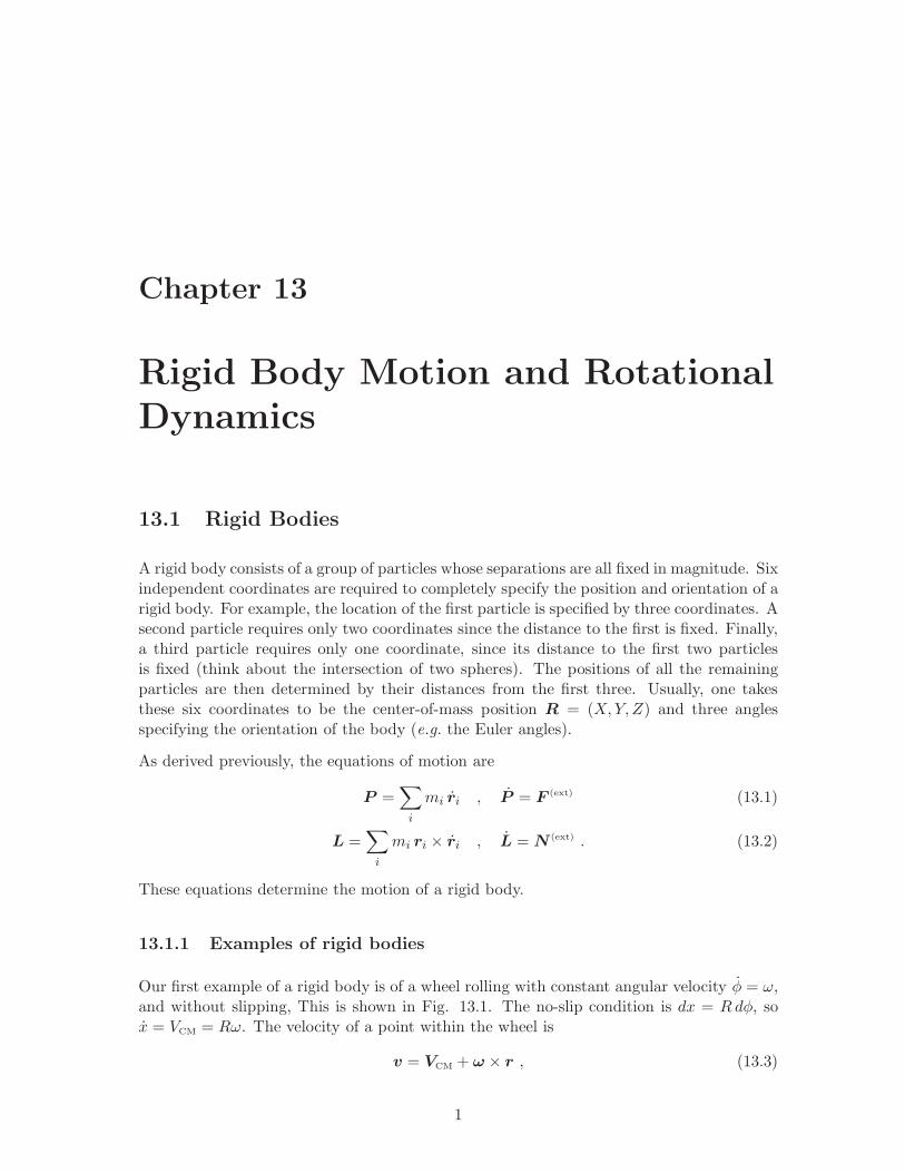
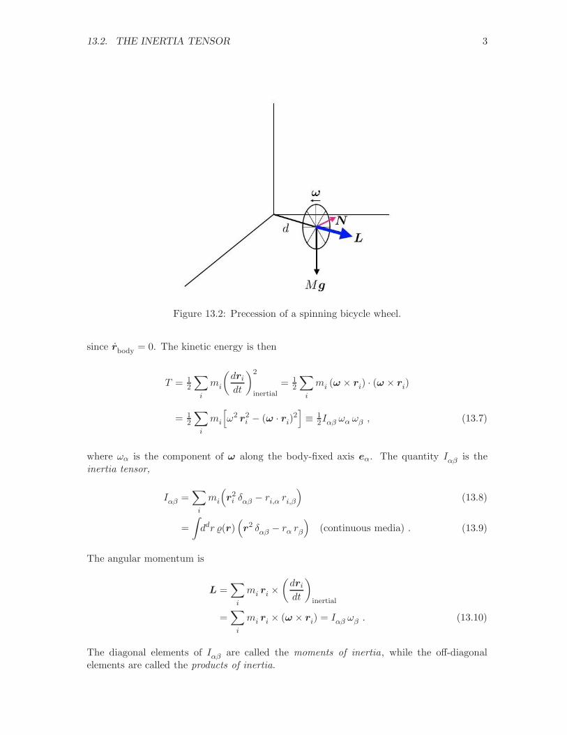
As a second example, consider a bicycle wheel of massM and radius R affixed to a light, firmrod of length d, as shown in Fig. 13.2. Assuming L lies in the (x, y) plane, one computesthe gravitational torque N = r × (Mg) = Mgd φ. The angular momentum vector thenrotates with angular frequency φ. Thus,
dφ =dL
L=⇒ φ =
Mgd
L. (13.4)
But L = MR2ω, so the precession frequency is
ωp = φ =gd
ωR2. (13.5)
For R = d = 30 cm and ω/2π = 200 rpm, find ωp/2π ≈ 15 rpm. Note that we have hereignored the contribution to L from the precession itself, which lies along z, resulting in thenutation of the wheel. This is justified if Lp/L = (d2/R2) · (ωp/ω) ≪ 1.
13.2 The Inertia Tensor
Suppose first that a point within the body itself is fixed. This eliminates the translationaldegrees of freedom from consideration. We now have
(dr
dt
)
inertial
= ω × r , (13.6)
13.2. THE INERTIA TENSOR 3
Figure 13.2: Precession of a spinning bicycle wheel.
since rbody = 0. The kinetic energy is then
T = 12
∑
i
mi
(dridt
)2
inertial
= 12
∑
i
mi (ω × ri) · (ω × ri)
= 12
∑
i
mi
[
ω2 r2i − (ω · ri)2
]
≡ 12Iαβ ωα ωβ , (13.7)
where ωα is the component of ω along the body-fixed axis eα. The quantity Iαβ is theinertia tensor,
Iαβ =∑
i
mi
(
r2i δαβ − ri,α ri,β
)
(13.8)
=
∫
ddr (r)(
r2 δαβ − rα rβ
)
(continuous media) . (13.9)
The angular momentum is
L =∑
i
mi ri ×(dridt
)
inertial
=∑
i
mi ri × (ω × ri) = Iαβ ωβ . (13.10)
The diagonal elements of Iαβ are called the moments of inertia, while the off-diagonalelements are called the products of inertia.
4 CHAPTER 13. RIGID BODY MOTION AND ROTATIONAL DYNAMICS
13.2.1 Coordinate transformations
Consider the basis transformation
e′α = Rαβ eβ . (13.11)
We demand e′α · e′β = δαβ , which means R ∈ O(d) is an orthogonal matrix, i.e. Rt = R−1.
Thus the inverse transformation is eα = Rtαβe
′
β . Consider next a general vector A = Aβ eβ .Expressed in terms of the new basis e′α, we have
A = Aβ
eβ︷ ︸︸ ︷
Rtβα e
′
α =
A′
α︷ ︸︸ ︷
RαβAβ e′
α (13.12)
Thus, the components of A transform as A′α = Rαβ Aβ . This is true for any vector.
Under a rotation, the density ρ(r) must satisfy ρ′(r′) = ρ(r). This is the transformationrule for scalars. The inertia tensor therefore obeys
I ′αβ =
∫
d3r′ ρ′(r′)[
r′2δαβ − r′α r
′
β
]
=
∫
d3r ρ(r)[
r2 δαβ −(Rαµrµ
)(Rβνrν
)]
= Rαµ Iµν Rtνβ . (13.13)
I.e. I ′ = RIRt, the transformation rule for tensors. The angular frequency ω is a vector, soω′α = Rαµ ωµ. The angular momentum L also transforms as a vector. The kinetic energy
is T = 12 ω
t · I · ω, which transforms as a scalar.
13.2.2 The case of no fixed point
If there is no fixed point, we can let r′ denote the distance from the center-of-mass (CM),which will serve as the instantaneous origin in the body-fixed frame. We then adopt thenotation where R is the CM position of the rotating body, as observed in an inertial frame,and is computed from the expression
R =1
M
∑
i
mi ρi =1
M
∫
d3r ρ(r) r , (13.14)
where the total mass is of course
M =∑
i
mi =
∫
d3r ρ(r) . (13.15)
The kinetic energy and angular momentum are then
T = 12MR
2 + 12Iαβ ωα ωβ (13.16)
Lα = ǫαβγMRβRγ + Iαβ ωβ , (13.17)
where Iαβ is given in eqs. 13.8 and 13.9, where the origin is the CM.
13.3. PARALLEL AXIS THEOREM 5
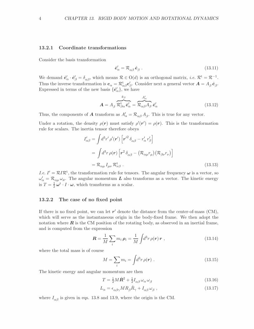
Figure 13.3: Application of the parallel axis theorem to a cylindrically symmetric massdistribution.
13.3 Parallel Axis Theorem
Suppose Iαβ is given in a body-fixed frame. If we displace the origin in the body-fixed frame
by d, then let Iαβ(d) be the inertial tensor with respect to the new origin. If, relative tothe origin at 0 a mass element lies at position r, then relative to an origin at d it will lie atr − d. We then have
Iαβ(d) =∑
i
mi
(r2i − 2d · ri + d2) δαβ − (ri,α − dα)(ri,β − dβ)
. (13.18)
If ri is measured with respect to the CM, then∑
i
mi ri = 0 (13.19)
andIαβ(d) = Iαβ(0) +M
(d2δαβ − dαdβ
), (13.20)
a result known as the parallel axis theorem.
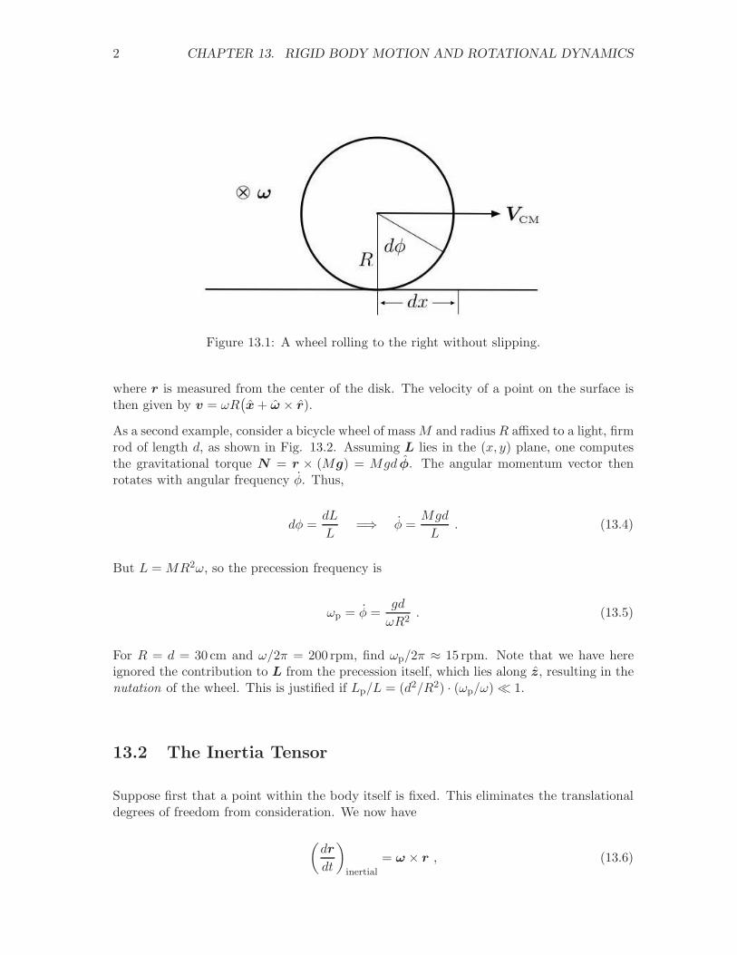
As an example of the theorem, consider the situation depicted in Fig. 13.3, where a cylin-drically symmetric mass distribution is rotated about is symmetry axis, and about an axistangent to its side. The component Izz of the inertia tensor is easily computed when theorigin lies along the symmetry axis:
Izz =
∫
d3r ρ(r) (r2 − z2) = ρL · 2πa∫
0
dr⊥r3⊥
= π2ρLa
4 = 12Ma2 , (13.21)
6 CHAPTER 13. RIGID BODY MOTION AND ROTATIONAL DYNAMICS
where M = πa2Lρ is the total mass. If we compute Izz about a vertical axis which istangent to the cylinder, the parallel axis theorem tells us that
I ′zz = Izz +Ma2 = 32Ma2 . (13.22)
Doing this calculation by explicit integration of∫dmr2
⊥would be tedious!
13.3.1 Example
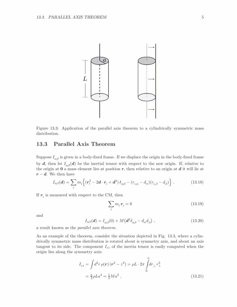
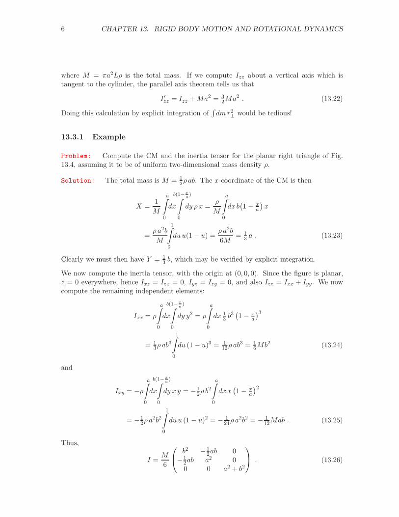
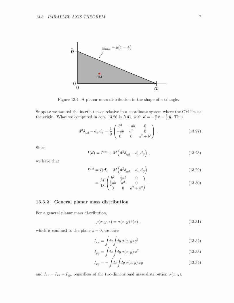
Problem: Compute the CM and the inertia tensor for the planar right triangle of Fig.13.4, assuming it to be of uniform two-dimensional mass density ρ.
Solution: The total mass is M = 12ρ ab. The x-coordinate of the CM is then
X =1
M
a∫
0
dx
b(1−xa)
∫
0
dy ρ x =ρ
M
a∫
0
dx b(1 − x
a
)x
=ρ a2b
M
1∫
0
duu(1 − u) =ρ a2b
6M= 1
3 a . (13.23)
Clearly we must then have Y = 13 b, which may be verified by explicit integration.
We now compute the inertia tensor, with the origin at (0, 0, 0). Since the figure is planar,z = 0 everywhere, hence Ixz = Izx = 0, Iyz = Izy = 0, and also Izz = Ixx + Iyy. We nowcompute the remaining independent elements:
Ixx = ρ
a∫
0
dx
b(1−xa)
∫
0
dy y2 = ρ
a∫
0
dx 13 b
3(1 − x
a
)3
= 13ρ ab
3
1∫
0
du (1 − u)3 = 112ρ ab
3 = 16Mb2 (13.24)
and
Ixy = −ρa∫
0
dx
b(1−xa)
∫
0
dy x y = −12ρ b
2
a∫
0
dxx(1 − x
a
)2
= −12ρ a
2b21∫
0
duu (1 − u)2 = − 124ρ a
2b2 = − 112Mab . (13.25)
Thus,
I =M
6
b2 −12ab 0
−12ab a2 00 0 a2 + b2
. (13.26)
13.3. PARALLEL AXIS THEOREM 7
Figure 13.4: A planar mass distribution in the shape of a triangle.
Suppose we wanted the inertia tensor relative in a coordinate system where the CM lies atthe origin. What we computed in eqn. 13.26 is I(d), with d = − a
3 x− b3 y. Thus,
d2δαβ − dα dβ =1
9
b2 −ab 0−ab a2 00 0 a2 + b2
. (13.27)
SinceI(d) = ICM +M
(
d2δαβ − dα dβ
)
, (13.28)
we have that
ICM = I(d) −M(
d2δαβ − dα dβ
)
(13.29)
=M
18
b2 12ab 0
12ab a2 00 0 a2 + b2
. (13.30)
13.3.2 General planar mass distribution
For a general planar mass distribution,
ρ(x, y, z) = σ(x, y) δ(z) , (13.31)
which is confined to the plane z = 0, we have
Ixx =
∫
dx
∫
dy σ(x, y) y2 (13.32)
Iyy =
∫
dx
∫
dy σ(x, y)x2 (13.33)
Ixy = −∫
dx
∫
dy σ(x, y)xy (13.34)
and Izz = Ixx + Iyy, regardless of the two-dimensional mass distribution σ(x, y).
8 CHAPTER 13. RIGID BODY MOTION AND ROTATIONAL DYNAMICS
13.4 Principal Axes of Inertia
We found that an orthogonal transformation to a new set of axes e′α = Rαβ eβ entails
I ′ = RIRt for the inertia tensor. Since I = It is manifestly a symmetric matrix, it canbe brought to diagonal form by such an orthogonal transformation. To find R, follow thisrecipe:
1. Find the diagonal elements of I ′ by setting P (λ) = 0, where
P (λ) = det(λ · 1 − I
), (13.35)
is the characteristic polynomial for I, and 1 is the unit matrix.
2. For each eigenvalue λa, solve the d equations∑
ν
Iµν ψaν = λa ψ
aµ . (13.36)
Here, ψaµ is the µth component of the ath eigenvector. Since (λ · 1 − I) is degenerate,these equations are linearly dependent, which means that the first d− 1 componentsmay be determined in terms of the dth component.
3. Because I = It, eigenvectors corresponding to different eigenvalues are orthogonal.In cases of degeneracy, the eigenvectors may be chosen to be orthogonal, e.g. via theGram-Schmidt procedure.
4. Due to the underdetermined aspect to step 2, we may choose an arbitrary normaliza-tion for each eigenvector. It is conventional to choose the eigenvectors to be orthonor-mal:
∑
µ ψaµ ψ
bµ = δab.
5. The matrix R is explicitly given by Raµ = ψaµ, the matrix whose row vectors are theeigenvectors ψa. Of course Rt is then the corresponding matrix of column vectors.
6. The eigenvectors form a complete basis. The resolution of unity may be expressed as∑
a
ψaµ ψaν = δµν . (13.37)
As an example, consider the inertia tensor for a general planar mass distribution, which isof the form
I =
Ixx Ixy 0Iyx Iyy 00 0 Izz
, (13.38)
where Iyx = Ixy and Izz = Ixx + Iyy. Define
A = 12
(Ixx + Iyy
)(13.39)
B =
√
14
(Ixx − Iyy
)2+ I2
xy (13.40)
ϑ = tan−1
(2Ixy
Ixx − Iyy
)
, (13.41)
13.5. EULER’S EQUATIONS 9
so that
I =
A+B cos ϑ B sinϑ 0B sinϑ A−B cos ϑ 0
0 0 2A
, (13.42)
The characteristic polynomial is found to be
P (λ) = (λ− 2A)[
(λ−A)2 −B2]
, (13.43)
which gives λ1 = A, λ2,3 = A±B. The corresponding normalized eigenvectors are
ψ1 =
001
, ψ2 =
cos 12ϑ
sin 12ϑ
0
, ψ3 =
− sin 12ϑ
cos 12ϑ
0
(13.44)
and therefore
R =
0 0 1cos 1
2ϑ sin 12ϑ 0
− sin 12ϑ cos 1
2ϑ 0
. (13.45)
13.5 Euler’s Equations
Let us now choose our coordinate axes to be the principal axes of inertia, with the CM atthe origin. We may then write
ω =
ω1
ω2
ω3
, I =
I1 0 00 I2 00 0 I3
=⇒ L =
I1 ω1
I2 ω2
I3 ω3
. (13.46)
The equations of motion are
N ext =
(dL
dt
)
inertial
=
(dL
dt
)
body
+ ω ×L
= I ω +ω × (I ω) .
Thus, we arrive at Euler’s equations:
I1 ω1 = (I2 − I3)ω2 ω3 +N ext1 (13.47)
I2 ω2 = (I3 − I1)ω3 ω1 +N ext2 (13.48)
I3 ω3 = (I1 − I2)ω1 ω2 +N ext3 . (13.49)
These are coupled and nonlinear. Also note the fact that the external torque must beevaluated along body-fixed principal axes. We can however make progress in the case
10 CHAPTER 13. RIGID BODY MOTION AND ROTATIONAL DYNAMICS
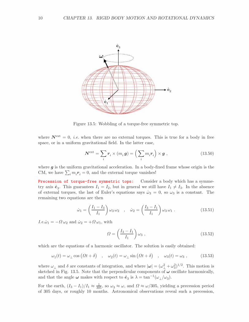
Figure 13.5: Wobbling of a torque-free symmetric top.
where N ext = 0, i.e. when there are no external torques. This is true for a body in freespace, or in a uniform gravitational field. In the latter case,
N ext =∑
i
ri × (mi g) =(∑
i
miri
)
× g , (13.50)
where g is the uniform gravitational acceleration. In a body-fixed frame whose origin is theCM, we have
∑
imiri = 0, and the external torque vanishes!
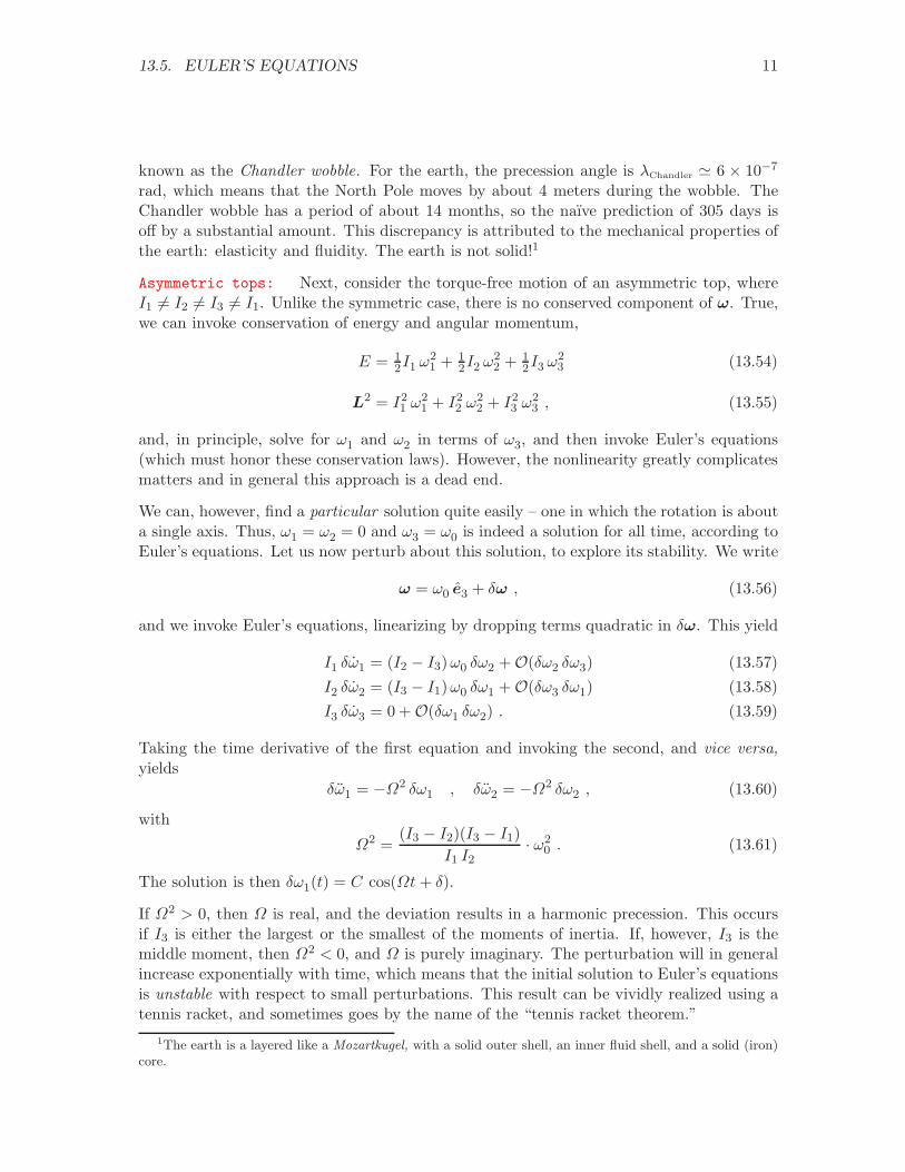
Precession of torque-free symmetric tops: Consider a body which has a symme-try axis e3. This guarantees I1 = I2, but in general we still have I1 6= I3. In the absenceof external torques, the last of Euler’s equations says ω3 = 0, so ω3 is a constant. Theremaining two equations are then
ω1 =
(I1 − I3I1
)
ω3 ω2 , ω2 =
(I3 − I1I1
)
ω3 ω1 . (13.51)
I.e.ω1 = −Ωω2 and ω2 = +Ωω1, with
Ω =
(I3 − I1I1
)
ω3 , (13.52)
which are the equations of a harmonic oscillator. The solution is easily obtained:
ω1(t) = ω⊥ cos(Ωt+ δ
), ω2(t) = ω⊥ sin
(Ωt+ δ
), ω3(t) = ω3 , (13.53)
where ω⊥
and δ are constants of integration, and where |ω| = (ω2⊥
+ω23)
1/2. This motion issketched in Fig. 13.5. Note that the perpendicular components of ω oscillate harmonically,and that the angle ω makes with respect to e3 is λ = tan−1(ω
⊥/ω3).
For the earth, (I3 − I1)/I1 ≈ 1305 , so ω3 ≈ ω, and Ω ≈ ω/305, yielding a precession period
of 305 days, or roughly 10 months. Astronomical observations reveal such a precession,
13.5. EULER’S EQUATIONS 11
known as the Chandler wobble. For the earth, the precession angle is λChandler ≃ 6 × 10⁻⁷
rad, which means that the North Pole moves by about 4 meters during the wobble. TheChandler wobble has a period of about 14 months, so the naıve prediction of 305 days isoff by a substantial amount. This discrepancy is attributed to the mechanical properties ofthe earth: elasticity and fluidity. The earth is not solid!1
Asymmetric tops: Next, consider the torque-free motion of an asymmetric top, whereI1 6= I2 6= I3 6= I1. Unlike the symmetric case, there is no conserved component of ω. True,we can invoke conservation of energy and angular momentum,
E = 12I1 ω
21 + 1
2I2 ω22 + 1
2I3 ω23 (13.54)
L2 = I21 ω
21 + I2
2 ω22 + I2
3 ω23 , (13.55)
and, in principle, solve for ω1 and ω2 in terms of ω3, and then invoke Euler’s equations(which must honor these conservation laws). However, the nonlinearity greatly complicatesmatters and in general this approach is a dead end.
We can, however, find a particular solution quite easily – one in which the rotation is abouta single axis. Thus, ω1 = ω2 = 0 and ω3 = ω0 is indeed a solution for all time, according toEuler’s equations. Let us now perturb about this solution, to explore its stability. We write
ω = ω0 e3 + δω , (13.56)
and we invoke Euler’s equations, linearizing by dropping terms quadratic in δω. This yield
I1 δω1 = (I2 − I3)ω0 δω2 + O(δω2 δω3) (13.57)
I2 δω2 = (I3 − I1)ω0 δω1 + O(δω3 δω1) (13.58)
I3 δω3 = 0 + O(δω1 δω2) . (13.59)
Taking the time derivative of the first equation and invoking the second, and vice versa,
yields
δω1 = −Ω2 δω1 , δω2 = −Ω2 δω2 , (13.60)
with
Ω2 =(I3 − I2)(I3 − I1)
I1 I2· ω2
0 . (13.61)
The solution is then δω1(t) = C cos(Ωt + δ).
If Ω2 > 0, then Ω is real, and the deviation results in a harmonic precession. This occursif I3 is either the largest or the smallest of the moments of inertia. If, however, I3 is themiddle moment, then Ω2 < 0, and Ω is purely imaginary. The perturbation will in generalincrease exponentially with time, which means that the initial solution to Euler’s equationsis unstable with respect to small perturbations. This result can be vividly realized using atennis racket, and sometimes goes by the name of the “tennis racket theorem.”
1The earth is a layered like a Mozartkugel, with a solid outer shell, an inner fluid shell, and a solid (iron)core.
12 CHAPTER 13. RIGID BODY MOTION AND ROTATIONAL DYNAMICS
13.5.1 Example
PROBLEM: A unsuspecting solid spherical planet of mass M0 rotates with angular velocityω0. Suddenly, a giant asteroid of mass αM0 smashes into and sticks to the planet at alocation which is at polar angle θ relative to the initial rotational axis. The new massdistribution is no longer spherically symmetric, and the rotational axis will precess. RecallEuler’s equation
dL
dt+ ω ×L = N ext (13.62)
for rotations in a body-fixed frame.
(a) What is the new inertia tensor Iαβ along principle center-of-mass frame axes? Don’t
forget that the CM is no longer at the center of the sphere! Recall I = 25MR2 for a solid
sphere.
(b) What is the period of precession of the rotational axis in terms of the original lengthof the day 2π/ω0?
SOLUTION: Let’s choose body-fixed axes with z pointing from the center of the planet tothe smoldering asteroid. The CM lies a distance
d =αM0 · R+M0 · 0
(1 + α)M0=
α
1 + αR (13.63)
from the center of the sphere. Thus, relative to the center of the sphere, we have
I = 25M0R
2
1 0 00 1 00 0 1
+ αM0R2
1 0 00 1 00 0 0
. (13.64)
Now we shift to a frame with the CM at the origin, using the parallel axis theorem,
Iαβ(d) = ICMαβ +M
(d2 δαβ − dαdβ
). (13.65)
Thus, with d = dz,
ICMαβ = 2
5M0R2
1 0 00 1 00 0 1
+ αM0R2
1 0 00 1 00 0 0
− (1 + α)M0d2
1 0 00 1 00 0 0
(13.66)
= M0R2
25 + α
1+α 0 0
0 25 + α
1+α 0
0 0 25
. (13.67)
13.6. EULER’S ANGLES 13
In the absence of external torques, Euler’s equations along principal axes read
I1dω1
dt= (I2 − I3)ω2 ω3
I2dω2
dt= (I3 − I1)ω3 ω1
I3dω3
dt= (I1 − I2)ω1 ω2
(13.68)
Since I1 = I2, ω3(t) = ω3(0) = ω0 cos θ is a constant. We then obtain ω1 = Ωω2, and
ω2 = −Ωω1, with
Ω =I2 − I3I1
ω3 =5α
7α + 2ω3 . (13.69)
The period of precession τ in units of the pre-cataclysmic day is
τ
T=ω
Ω=
7α + 2
5α cos θ. (13.70)
13.6 Euler’s Angles
In d dimensions, an orthogonal matrix R ∈ O(d) has 12d(d − 1) independent parameters.
To see this, consider the constraint RtR = 1. The matrix RtR is manifestly symmetric,so it has 1
2d(d + 1) independent entries (e.g. on the diagonal and above the diagonal).This amounts to 1
2d(d + 1) constraints on the d2 components of R, resulting in 12d(d − 1)
freedoms. Thus, in d = 3 rotations are specified by three parameters. The Euler angles
φ, θ, ψ provide one such convenient parameterization.
A general rotation R(φ, θ, ψ) is built up in three steps. We start with an orthonormal triade0µ of body-fixed axes. The first step is a rotation by an angle φ about e0
3:
e′µ = Rµν
(e0
3, φ)e0ν , R
(e0
3, φ)
=
cosφ sinφ 0− sinφ cosφ 0
0 0 1
(13.71)
This step is shown in panel (a) of Fig. 13.6. The second step is a rotation by θ about thenew axis e′1:
e′′µ = Rµν
(e′1, θ
)e′ν , R
(e′1, θ
)=
1 0 00 cos θ sin θ0 − sin θ cos θ
(13.72)
This step is shown in panel (b) of Fig. 13.6. The third and final step is a rotation by ψabout the new axis e′′3 :
e′′′µ = Rµν
(e′′3 , ψ
)e′′ν , R
(e′′3 , ψ
)=
cosψ sinψ 0− sinψ cosψ 0
0 0 1
(13.73)
14 CHAPTER 13. RIGID BODY MOTION AND ROTATIONAL DYNAMICS
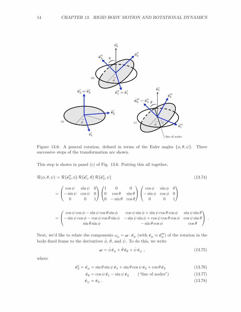
Figure 13.6: A general rotation, defined in terms of the Euler angles φ, θ, ψ. Threesuccessive steps of the transformation are shown.
This step is shown in panel (c) of Fig. 13.6. Putting this all together,
R(φ, θ, ψ) = R(e′′3 , φ
)R(e′1, θ
)R(e0
3, ψ)
(13.74)
=
cosψ sinψ 0− sinψ cosψ 0
0 0 1
1 0 00 cos θ sin θ0 − sin θ cos θ
cosφ sinφ 0− sinφ cosφ 0
0 0 1
=
cosψ cosφ− sinψ cos θ sinφ cosψ sinφ+ sinψ cos θ cosφ sinψ sin θ− sinψ cosφ− cosψ cos θ sinφ − sinψ sinφ+ cosψ cos θ cosφ cosψ sin θ
sin θ sinφ − sin θ cosφ cos θ
.
Next, we’d like to relate the components ωµ = ω · eµ (with eµ ≡ e′′′µ ) of the rotation in the
body-fixed frame to the derivatives φ, θ, and ψ. To do this, we write
ω = φ eφ + θ eθ + ψ eψ , (13.75)
where
e03 = eφ = sin θ sinψ e1 + sin θ cosψ e2 + cos θ e3 (13.76)
eθ = cosψ e1 − sinψ e2 (“line of nodes”) (13.77)
eψ = e3 . (13.78)
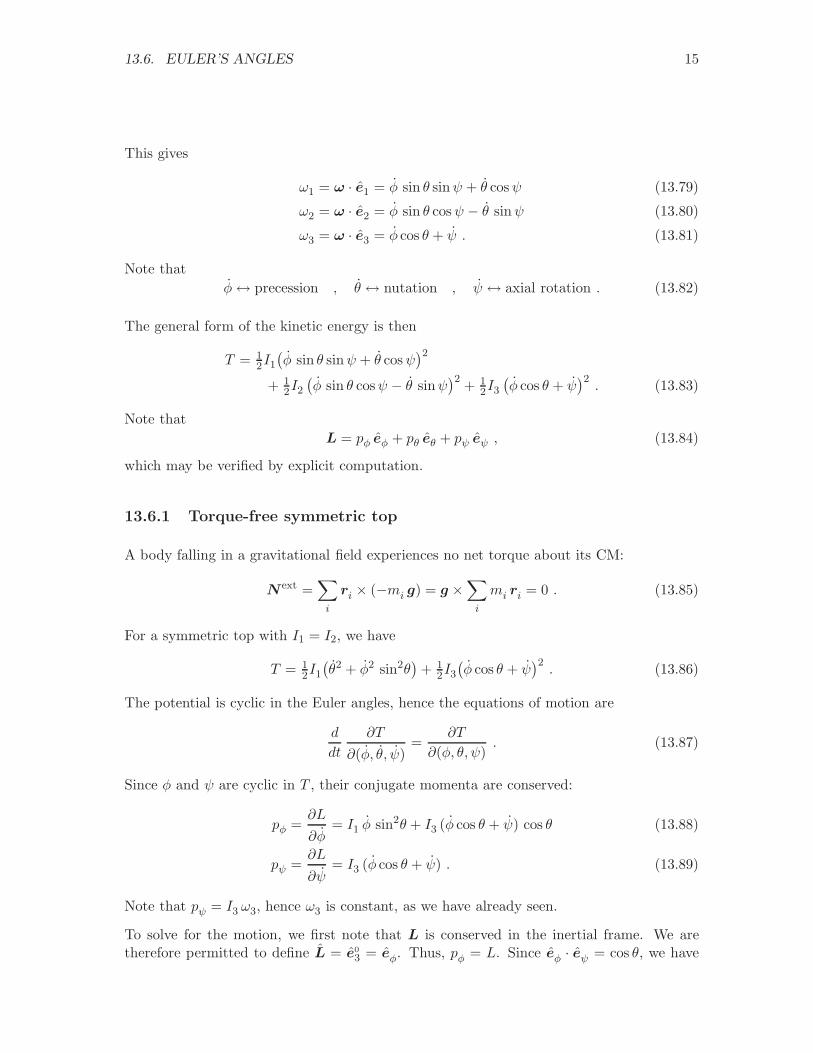
13.6. EULER’S ANGLES 15
This gives
ω1 = ω · e1 = φ sin θ sinψ + θ cosψ (13.79)
ω2 = ω · e2 = φ sin θ cosψ − θ sinψ (13.80)
ω3 = ω · e3 = φ cos θ + ψ . (13.81)
Note that
φ↔ precession , θ ↔ nutation , ψ ↔ axial rotation . (13.82)
The general form of the kinetic energy is then
T = 12I1(φ sin θ sinψ + θ cosψ
)2
+ 12I2(φ sin θ cosψ − θ sinψ
)2+ 1
2I3(φ cos θ + ψ
)2. (13.83)
Note that
L = pφ eφ + pθ eθ + pψ eψ , (13.84)
which may be verified by explicit computation.
13.6.1 Torque-free symmetric top
A body falling in a gravitational field experiences no net torque about its CM:
N ext =∑
i
ri × (−mi g) = g ×∑
i
mi ri = 0 . (13.85)
For a symmetric top with I1 = I2, we have
T = 12I1(θ2 + φ2 sin2θ
)+ 1
2I3(φ cos θ + ψ
)2. (13.86)
The potential is cyclic in the Euler angles, hence the equations of motion are
d
dt
∂T
∂(φ, θ, ψ)=
∂T
∂(φ, θ, ψ). (13.87)
Since φ and ψ are cyclic in T , their conjugate momenta are conserved:
pφ =∂L
∂φ= I1 φ sin2θ + I3 (φ cos θ + ψ) cos θ (13.88)
pψ =∂L
∂ψ= I3 (φ cos θ + ψ) . (13.89)
Note that pψ = I3 ω3, hence ω3 is constant, as we have already seen.
To solve for the motion, we first note that L is conserved in the inertial frame. We aretherefore permitted to define L = e0
3 = eφ. Thus, pφ = L. Since eφ · eψ = cos θ, we have
16 CHAPTER 13. RIGID BODY MOTION AND ROTATIONAL DYNAMICS
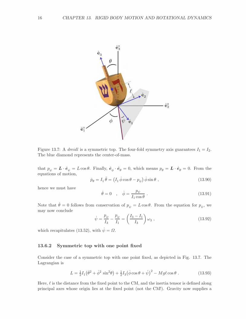
Figure 13.7: A dreidl is a symmetric top. The four-fold symmetry axis guarantees I1 = I2.The blue diamond represents the center-of-mass.
that pψ = L · eψ = L cos θ. Finally, eφ · eθ = 0, which means pθ = L · eθ = 0. From theequations of motion,
pθ = I1 θ =(I1 φ cos θ − pψ
)φ sin θ , (13.90)
hence we must have
θ = 0 , φ =pψ
I1 cos θ. (13.91)
Note that θ = 0 follows from conservation of pψ = L cos θ. From the equation for pψ, wemay now conclude
ψ =pψI3
−pψI1
=
(I3 − I1I3
)
ω3 , (13.92)
which recapitulates (13.52), with ψ = Ω.
13.6.2 Symmetric top with one point fixed
Consider the case of a symmetric top with one point fixed, as depicted in Fig. 13.7. TheLagrangian is
L = 12I1(θ2 + φ2 sin2θ
)+ 1
2I3(φ cos θ + ψ
)2 −Mgℓ cos θ . (13.93)
Here, ℓ is the distance from the fixed point to the CM, and the inertia tensor is defined alongprincipal axes whose origin lies at the fixed point (not the CM!). Gravity now supplies a
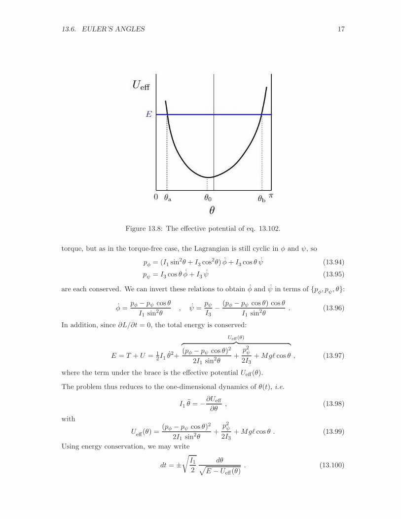
13.6. EULER’S ANGLES 17
Figure 13.8: The effective potential of eq. 13.102.
torque, but as in the torque-free case, the Lagrangian is still cyclic in φ and ψ, so
pφ = (I1 sin2θ + I3 cos2θ) φ+ I3 cos θ ψ (13.94)
pψ = I3 cos θ φ+ I3 ψ (13.95)
are each conserved. We can invert these relations to obtain φ and ψ in terms of pφ, pψ, θ:
φ =pφ − pψ cos θ
I1 sin2θ, ψ =
pψI3
− (pφ − pψ cos θ) cos θ
I1 sin2θ. (13.96)
In addition, since ∂L/∂t = 0, the total energy is conserved:
E = T + U = 12I1 θ
2+
Ueff (θ)︷ ︸︸ ︷
(pφ − pψ cos θ)2
2I1 sin2θ+p2ψ
2I3+Mgℓ cos θ , (13.97)
where the term under the brace is the effective potential Ueff(θ).
The problem thus reduces to the one-dimensional dynamics of θ(t), i.e.
I1 θ = −∂Ueff
∂θ, (13.98)
with
Ueff(θ) =(pφ − pψ cos θ)2
2I1 sin2θ+p2ψ
2I3+Mgℓ cos θ . (13.99)
Using energy conservation, we may write
dt = ±√
I12
dθ√
E − Ueff(θ). (13.100)
18 CHAPTER 13. RIGID BODY MOTION AND ROTATIONAL DYNAMICS
and thus the problem is reduced to quadratures:
t(θ) = t(θ0) ±√
I12
θ∫
θ0
dϑ1
√
E − Ueff(ϑ). (13.101)
We can gain physical insight into the motion by examining the shape of the effective po-tential,
Ueff(θ) =(pφ − pψ cos θ)2
2I1 sin2θ+Mgℓ cos θ +
p2ψ
2I3, (13.102)
over the interval θ ∈ [0, π]. Clearly Ueff(0) = Ueff(π) = ∞, so the motion must be bounded.What is not yet clear, but what is nonetheless revealed by some additional analysis, is thatUeff(θ) has a single minimum on this interval, at θ = θ0. The turning points for the θ motionare at θ = θa and θ = θb, where Ueff(θa) = Ueff(θb) = E. Clearly if we expand about θ0 andwrite θ = θ0 + η, the η motion will be harmonic, with
η(t) = η0 cos(Ωt+ δ) , Ω =
√
U ′′
eff(θ0)
I1. (13.103)
To prove that Ueff(θ) has these features, let us define u ≡ cos θ. Then u = − θ sin θ, and
from E = 12I1 θ
2 + Ueff(θ) we derive
u2 =
(2E
I1−
p2ψ
I1I3
)
(1 − u2) − 2Mgℓ
I1(1 − u2)u−
(pφ − pψ u
I1
)2
≡ f(u) . (13.104)
The turning points occur at f(u) = 0. The function f(u) is cubic, and the coefficient of the
cubic term is 2Mgℓ/I1, which is positive. Clearly f(u = ±1) = −(pφ∓ pψ)2/I21 is negative,
so there must be at least one solution to f(u) = 0 on the interval u ∈ (1,∞). Clearly therecan be at most three real roots for f(u), since the function is cubic in u, hence there are at
most two turning points on the interval u ∈ [−1, 1]. Thus, Ueff(θ) has the form depicted infig. 13.8.
To apprehend the full motion of the top in an inertial frame, let us follow the symmetryaxis e3:
e3 = sin θ sinφ e01 − sin θ cosφ e0
2 + cos θ e03 . (13.105)
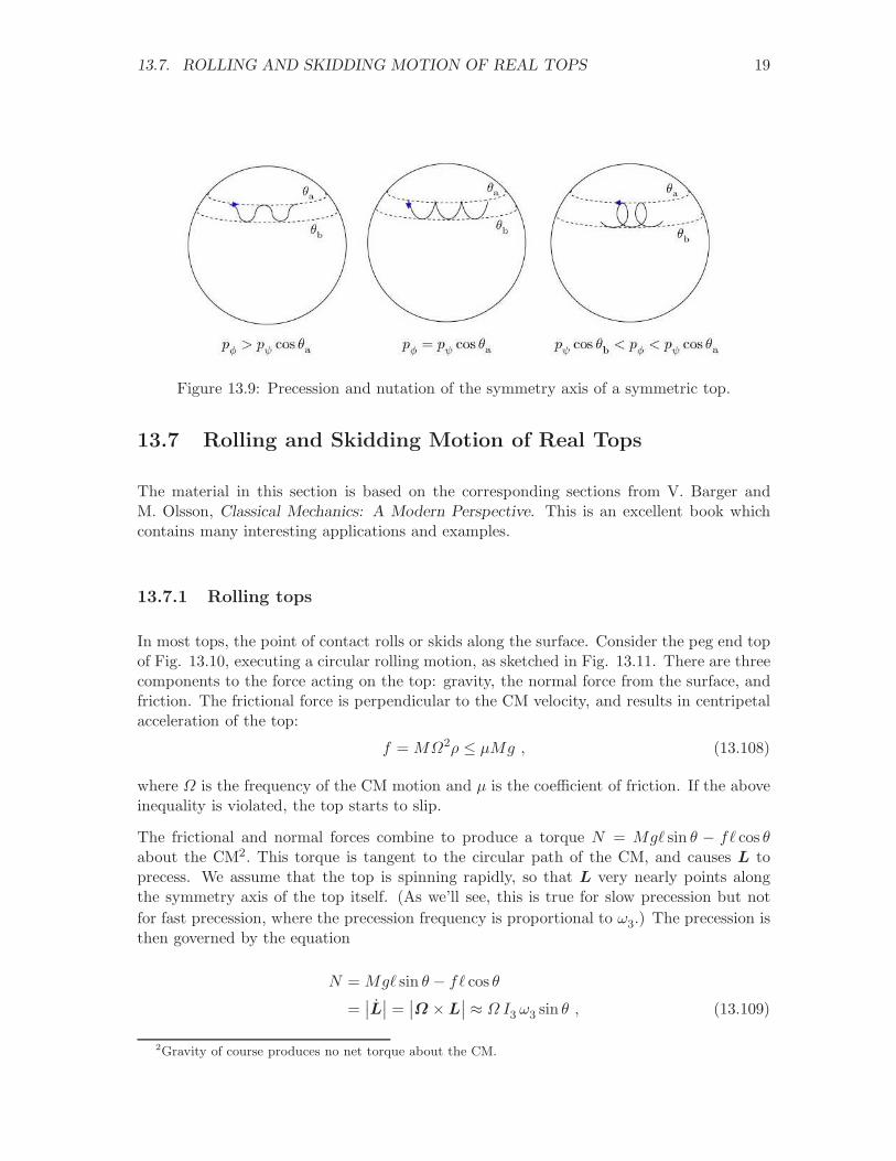
Once we know θ(t) and φ(t) we’re done. The motion θ(t) is described above: θ oscillatesbetween turning points at θa and θb. As for φ(t), we have already derived the result
φ =pφ − pψ cos θ
I1 sin2θ. (13.106)
Thus, if pφ > pψ cos θa, then φ will remain positive throughout the motion. If, on the otherhand, we have
pψ cos θb < pφ < pψ cos θa , (13.107)
then φ changes sign at an angle θ∗ = cos−1(pφ/pψ
). The motion is depicted in Fig. 13.9.
An extensive discussion of this problem is given in H. Goldstein, Classical Mechanics.
13.7. ROLLING AND SKIDDING MOTION OF REAL TOPS 19
Figure 13.9: Precession and nutation of the symmetry axis of a symmetric top.
13.7 Rolling and Skidding Motion of Real Tops
The material in this section is based on the corresponding sections from V. Barger andM. Olsson, Classical Mechanics: A Modern Perspective. This is an excellent book whichcontains many interesting applications and examples.
13.7.1 Rolling tops
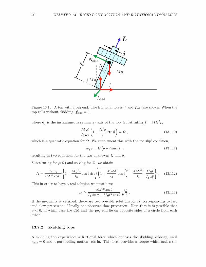
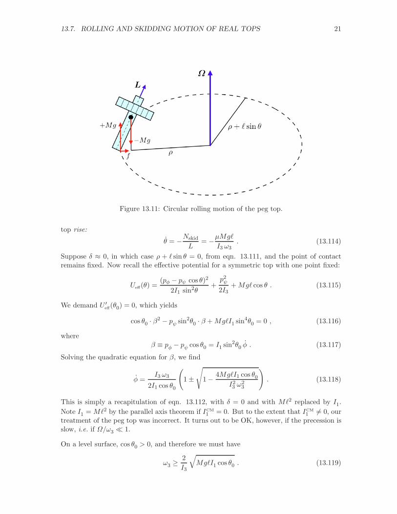
In most tops, the point of contact rolls or skids along the surface. Consider the peg end topof Fig. 13.10, executing a circular rolling motion, as sketched in Fig. 13.11. There are threecomponents to the force acting on the top: gravity, the normal force from the surface, andfriction. The frictional force is perpendicular to the CM velocity, and results in centripetalacceleration of the top:
f = MΩ2ρ ≤ µMg , (13.108)
where Ω is the frequency of the CM motion and µ is the coefficient of friction. If the aboveinequality is violated, the top starts to slip.
The frictional and normal forces combine to produce a torque N = Mgℓ sin θ − fℓ cos θabout the CM2. This torque is tangent to the circular path of the CM, and causes L toprecess. We assume that the top is spinning rapidly, so that L very nearly points alongthe symmetry axis of the top itself. (As we’ll see, this is true for slow precession but not
for fast precession, where the precession frequency is proportional to ω3.) The precession isthen governed by the equation
N = Mgℓ sin θ − fℓ cos θ
=∣∣L∣∣ =
∣∣Ω ×L
∣∣ ≈ Ω I3 ω3 sin θ , (13.109)
2Gravity of course produces no net torque about the CM.
20 CHAPTER 13. RIGID BODY MOTION AND ROTATIONAL DYNAMICS
Figure 13.10: A top with a peg end. The frictional forces f and fskid are shown. When thetop rolls without skidding, fskid = 0.
where e3 is the instantaneous symmetry axis of the top. Substituting f = MΩ2ρ,
Mgℓ
I3 ω3
(
1 − Ω2ρ
gctn θ
)
= Ω , (13.110)
which is a quadratic equation for Ω. We supplement this with the ‘no slip’ condition,
ω3 δ = Ω(ρ+ ℓ sin θ
), (13.111)
resulting in two equations for the two unknowns Ω and ρ.
Substituting for ρ(Ω) and solving for Ω, we obtain
Ω =I3 ω3
2Mℓ2 cos θ
1 +Mgℓδ
I3ctn θ ±
√(
1 +Mgℓδ
I3ctn θ
)2
− 4Mℓ2
I3· Mgℓ
I3 ω23
. (13.112)
This in order to have a real solution we must have
ω3 ≥ 2Mℓ2 sin θ
I3 sin θ +Mgℓδ cos θ
√g
ℓ. (13.113)
If the inequality is satisfied, there are two possible solutions for Ω, corresponding to fastand slow precession. Usually one observes slow precession. Note that it is possible thatρ < 0, in which case the CM and the peg end lie on opposite sides of a circle from eachother.
13.7.2 Skidding tops
A skidding top experiences a frictional force which opposes the skidding velocity, untilvskid = 0 and a pure rolling motion sets in. This force provides a torque which makes the
13.7. ROLLING AND SKIDDING MOTION OF REAL TOPS 21
Figure 13.11: Circular rolling motion of the peg top.
top rise:
θ = −Nskid
L= −µMgℓ
I3 ω3. (13.114)
Suppose δ ≈ 0, in which case ρ + ℓ sin θ = 0, from eqn. 13.111, and the point of contactremains fixed. Now recall the effective potential for a symmetric top with one point fixed:
Ueff(θ) =(pφ − pψ cos θ)2
2I1 sin2θ+p2ψ
2I3+Mgℓ cos θ . (13.115)
We demand U ′eff(θ0) = 0, which yields
cos θ0 · β2 − pψ sin2θ0 · β +MgℓI1 sin4θ0 = 0 , (13.116)
whereβ ≡ pφ − pψ cos θ0 = I1 sin2θ0 φ . (13.117)
Solving the quadratic equation for β, we find
φ =I3 ω3
2I1 cos θ0
(
1 ±
√
1 − 4MgℓI1 cos θ0I23 ω
23
)
. (13.118)
This is simply a recapitulation of eqn. 13.112, with δ = 0 and with Mℓ2 replaced by I1.
Note I1 = Mℓ2 by the parallel axis theorem if ICM1 = 0. But to the extent that ICM
1 6= 0, ourtreatment of the peg top was incorrect. It turns out to be OK, however, if the precession isslow, i.e. if Ω/ω3 ≪ 1.
On a level surface, cos θ0 > 0, and therefore we must have
ω3 ≥ 2
I3
√
MgℓI1 cos θ0 . (13.119)
22 CHAPTER 13. RIGID BODY MOTION AND ROTATIONAL DYNAMICS
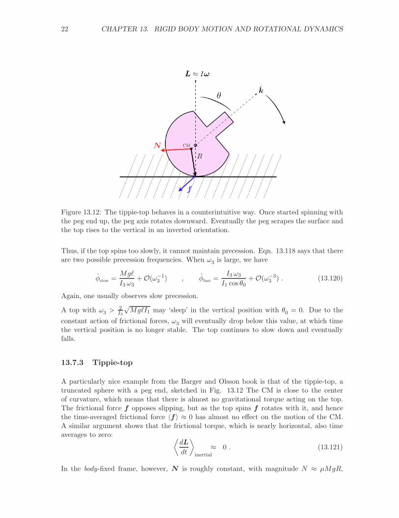
Figure 13.12: The tippie-top behaves in a counterintuitive way. Once started spinning withthe peg end up, the peg axis rotates downward. Eventually the peg scrapes the surface andthe top rises to the vertical in an inverted orientation.
Thus, if the top spins too slowly, it cannot maintain precession. Eqn. 13.118 says that thereare two possible precession frequencies. When ω3 is large, we have
φslow =Mgℓ
I3 ω3+ O(ω−1
3 ) , φfast =I3 ω3
I1 cos θ0+ O(ω−3
3 ) . (13.120)
Again, one usually observes slow precession.
A top with ω3 >2I3
√MgℓI1 may ‘sleep’ in the vertical position with θ0 = 0. Due to the
constant action of frictional forces, ω3 will eventually drop below this value, at which timethe vertical position is no longer stable. The top continues to slow down and eventuallyfalls.
13.7.3 Tippie-top
A particularly nice example from the Barger and Olsson book is that of the tippie-top, atruncated sphere with a peg end, sketched in Fig. 13.12 The CM is close to the centerof curvature, which means that there is almost no gravitational torque acting on the top.The frictional force f opposes slipping, but as the top spins f rotates with it, and hencethe time-averaged frictional force 〈f〉 ≈ 0 has almost no effect on the motion of the CM.A similar argument shows that the frictional torque, which is nearly horizontal, also timeaverages to zero: ⟨
dL
dt
⟩
inertial
≈ 0 . (13.121)
In the body-fixed frame, however, N is roughly constant, with magnitude N ≈ µMgR,
13.7. ROLLING AND SKIDDING MOTION OF REAL TOPS 23
where R is the radius of curvature and µ the coefficient of sliding friction. Now we invoke
N =dL
dt
∣∣∣∣body
+ ω ×L . (13.122)
The second term on the RHS is very small, because the tippie-top is almost spherical, henceinertia tensor is very nearly diagonal, and this means
ω ×L ≈ ω × Iω = 0 . (13.123)
Thus, Lbody ≈ N , and taking the dot product of this equation with the unit vector k, weobtain
−N sin θ = k ·N =d
dt
(
k · Lbody
)
= −L sin θ θ . (13.124)
Thus,
θ =N
L≈ µMgR
Iω. (13.125)
Once the stem scrapes the table, the tippie-top rises to the vertical just like any other risingtop.