RIGOROUS MATHEMATICAL MODELING OF ADSORPTION …

1

Grant No. FA8655-04-1-3053

RIGOROUS MATHEMATICAL MODELING OF ADSORPTION SYSTEM WITH ELECTROTHERMAL

REGENERATION OF THE USED ADSORBENT

Principal investigator:

Dr. Menka Petkovska

Department of Chemical Engineering, Faculty of Technology and Metallurgy, University of Belgrade, Serbia and Montenegro

Other participants on the project: Danijela Antov-Bozalo, Graduate student

Ana Markovic, Graduate student

Final Performance Report for Year 2

FEMLAB modeling of complete TSA cycles for adsorbers with one and two annular, radial-flow cartridges

Report Documentation Page Form ApprovedOMB No. 0704-0188

Public reporting burden for the collection of information is estimated to average 1 hour per response, including the time for reviewing instructions, searching existing data sources, gathering andmaintaining the data needed, and completing and reviewing the collection of information. Send comments regarding this burden estimate or any other aspect of this collection of information,including suggestions for reducing this burden, to Washington Headquarters Services, Directorate for Information Operations and Reports, 1215 Jefferson Davis Highway, Suite 1204, ArlingtonVA 22202-4302. Respondents should be aware that notwithstanding any other provision of law, no person shall be subject to a penalty for failing to comply with a collection of information if itdoes not display a currently valid OMB control number.

1. REPORT DATE 28 JUL 2005

2. REPORT TYPE N/A

3. DATES COVERED

4. TITLE AND SUBTITLE Rigorous Mathematical Modeling of an Adsorption System WithElectrothermal Regeneration of the Used Adsorbent

5a. CONTRACT NUMBER

5b. GRANT NUMBER

5c. PROGRAM ELEMENT NUMBER

6. AUTHOR(S) 5d. PROJECT NUMBER

5e. TASK NUMBER

5f. WORK UNIT NUMBER

7. PERFORMING ORGANIZATION NAME(S) AND ADDRESS(ES) University of Belgrade Faculty on Technology and Metallurgy Belgrade11000 Yugoslavia

8. PERFORMING ORGANIZATIONREPORT NUMBER

9. SPONSORING/MONITORING AGENCY NAME(S) AND ADDRESS(ES) 10. SPONSOR/MONITOR’S ACRONYM(S)

11. SPONSOR/MONITOR’S REPORT NUMBER(S)

12. DISTRIBUTION/AVAILABILITY STATEMENT Approved for public release, distribution unlimited.

13. SUPPLEMENTARY NOTES The original document contains color images.

14. ABSTRACT

15. SUBJECT TERMS

16. SECURITY CLASSIFICATION OF: 17. LIMITATION OF ABSTRACT

UU

18. NUMBEROF PAGES

58

19a. NAME OFRESPONSIBLE PERSON

a. REPORT unclassified

b. ABSTRACT unclassified

c. THIS PAGE unclassified

Standard Form 298 (Rev. 8-98) Prescribed by ANSI Std Z39-18

2

PROJECT OVERVIEW

OBJECTIVES The general objective of the project is fundamental mathematical modeling of a complex TSA system with electrothermal desorption step, with adsorbers assembled of one or more activated carbon fiber clot (ACFC) cartridge-type, radial flow fixed beds and with in-vessel condensation of the desorbed vapor. During the first stage of the project, a mathematical model of a single cartridge without condensation was developed and used for simulation.

The objective of this, second stage of the project, is to model the complete TSA system, for adsorbers with one and more cartridges. Besides the material and energy balances, these models have to include the momentum balances, in order to define the complex gas flow in the complex geometry of the adsorber. The models have to describe adsorption, electrothermal desorption and electrothermal desorption accompanied with condensation of the desorbed vapor, as well as the complete TSA cycle. These models will be used for prediction of the velocity, pressure, concentration and temperature profiles in the adsorbers and calculation of the mass of condensed liquid and used electric energy. Applicability of the developed mathematical models for optimization of the TSA process, with regard to the separation and purification factor, regeneration of the condensed vapor and used energy, will also be investigated.

STATUS OF EFFORT Models for two types of adsorbers, one with only one, and the other with two cartridges, have been developed in this stage. These adsorber types will be called 1-cartridge and 2-cartridges adsorber, respectively, through this manuscript. For each adsorber type, three models were built, in order to describe three stages of a compete TSA cycle: adsorption, electrothermal desorption and electrothermal desorption with in-vessel condensation. These models were built using Femlab, a specialized software tool for modeling of complex systems with complex geometry. In order to describe the complete TSA cycle, the models for the three stages were integrated, by using a combination of Femlab and Matlab. The models were successfully used for simulation of separate stages of the process and of the complete TSA cycles, as well as for their optimization.

ACCOMPLISHMENTS /NEW FINDINGS

The accomplishments of this project can be perceived from two aspects:

1. The developed models represent a mathematical tool which can be used for simulation of the investigated TSA system, its analysis, predicting of the concentration and temperature profiles in the system and its optimization. This was the main objective of this project.

2. By developing Femlab and combined Femlab/Matlab models of this, very complex system, involving a number of coupled processes and phenomena taking place in a complex geometry, a progress in the Femlab and Femlab/Matlab modeling has been achieved.

3

PERSONNEL SUPPORTED Danijela Antov-Bozalo, Graduate student

Ana Markovic, Graduate student

Dr. Menka Petkovska, Professor

PUBLICATIONS 1. M. Petkovska, D. Antov and P. Sullivan, “Electrothermal desorption in an annular -

radial flow – ACFC adsorber – Mathematical modeling”, Adsorption, 11, 585-590, 2005. (also presented at the FOA-8, 8th International Conference on Fundamentals of Adsorption (FOA8), Sedona, USA, May 23-28, 2004)

In preparation: One journal paper and 2 conference papers

NEW DISCOVERYS, INVENTIONS AND PATENTS: None

4

DETAILED REPORT

1. Introduction The idea about regeneration of used adsorbents by direct heating of the adsorbent particles by passing electric current through them (Joule effect), was first published in the 1970s [1]. Desorption process based on this principle was later named electrothermal desorption [2]. It was recognized as a prospective way to perform desorption steps of TSA cycles. At the same time, fibrous activated carbon was recognized as a very convenient adsorbent form for its realization. Electrothermal desorption has some advantages over conventional methods, regarding adsorption kinetics and dynamics [3, 4] and energy efficiency [2, 5]. Some industrial applications of electrothermal desorption have been reported recently [6, 7]. Nevertheless, the development of mathematical description of processes based on electrothermal desorption hasn’t been following the development of the process itself, so far.

A new TSA process with electrothermal desorption step, based on adsorbers assembled of one or more annular, cartridge-type, fixed-beds, with in-vessel condensation, has been presented recently [5, 8, 9]. Its schematic representation is given in Figure 1.

The aim of this project is to develop a rigorous, fundamental mathematical model of this system, which could be used for simulation, analysis and optimization of the TSA process developed by Sullivan [5].

1.1. Description of the system

The adsorbers of the TSA system shown in Figure 1 are composed of one or more annular, radial-flow cartridge-type adsorbent beds. A single cartridge is schematically shown in Figure 2. It is formed as a cylindrical roll of activated carbon fiber cloth (ACFC), spirally coiled around a porous central pipe. The gas flow through the adsorber is in the radial direction. During the desorption step, electric current is passed through the activated carbon cloth in the axial direction, causing heat generation, heating of the adsorbent and desorption.

Figure 2. Schematic representation of the annular - radial flow - ACFC adsorbent bed

Figure 1. Overall schematic representation of the ACFC adsorption – rapid electrothermal desorption system (from Ref. [5])

5

The cartridges are situated in a cylindrical adsorber vessel. During desorption, the hot gas steam rich with the desorbed vapor comes into contact with the cold vessel wall and the vapor condenses. In that way, the adsorber vessel serves as a passive condenser. The bottom outlet of the adsorber vessel is funnel-shaped, in order to facilitate draining of the condensed liquid.

In this phase of the project, adsorbers with one and two cartridges will be modeled. The 1-cartridge adsorber is shown in Figure 3 and the 2-cartridges adsorber in Figure 4.

In Figures 3 and 4 the directions of the fluid flow are also shown, in order to clarify the processes:

- For the 1-cartridge adsorber the flow directions during adsorption and desorption are the same: the gas enters the adsorber through the central tube, from the bottom, and, after passing through the adsorbent bed in the radial direction, exits from the annular space around the adsorbent bed through the funnel-shaped bottom outlet. During desorption, the desorbed vapor is partially condensed at the cold outer wall of the adsorber, and the outlet stream contains both gas and the condensed liquid.

- For the 2-cartridges adsorber, the flow directions during adsorption and desorption are somewhat different. During adsorption the feed stream enters the adsorber from the bottom, through the

central tube of the bottom cartridge, and the purified stream exits the adsorber at the top, through the central tube of the top cartridge (Fig. 4A). Between the inlet and the outlet, the stream flows through both adsorbent beds in the radial direction, but in the opposite directions (through the bottom cartridge from the center to the periphery, and through the top cartridge from the periphery to the center). During desorption, two inert streams are introduced into the adsorber, from the bottom and the top, through the central tubes of both cartridges, and the gas and the condensed liquid exit the adsorber through the funnel shaped bottom outlet of the annular tube around the cartridges (Fig 4B). It should be noticed that the gas cannot flow directly between the central tubes of the top and the bottom cartridge. Also, the electric current supply for the two cartridges is separate.

The inlet gas flow-rate during adsorption is generally several times higher than during desorption. The inlet gas during desorption is pure inert.

1.2. Brief survey of the first-year results

During the first year, the modeling efforts were concentrated on modeling of a single annular, cartridge-type, fixed-bed adsorber, without condensation. Two deterministic models were postulated: the first one assuming uniform adsorbent density throughout the adsorbent bed, and the second one taking into account the structure of the bed made of layers of ACFC. Both models were obtained as complex sets of coupled nonlinear PDEs, ODEs and algebraic equations. Numerical procedures for solving the model equations were established and used for simulation of adsorption, electroresistive heating, electrothermal desorption and consecutive adsorption-desorption, using Matlab software. Similar results were obtained with the two models. The results of this stage are presented in the Final Performance Report for project FA8655-03-1-3010 [10].

Figure 3. 1-cartridge adsorber

Figure 4. 2-cartridge adsorber: (A) adsorption, (B) desorption

6

1.3. Outline of the second year project

The TSA system defined in Ref. [5] is very complex, regarding both its geometry and the processes involved. For that reason, a decision was made to perform the modeling of the complete system by using some specialized modeling software. Our choice was to use FEMLAB, relatively new modeling software based on the finite-element method for solving partial differential model equations.

Analysis of the TSA system with electrothermal desorption and in-vessel condensation shows that the complete cycle can be broken down into three consecutive steps:

- adsorption,

- desorption without condensation,

- desorption accompanied with condensation.

Although these three stages can be described by the same set of model equations, the boundary conditions corresponding to the three stages are essentially different, so three different Femlab models need to be built. In order to simulate a complete TSA cycle, these 3 models have to be run in consequence with automatically switching from one model to the next, when predefined conditions are reached. The most convenient way to achieve that is to build a combined Femlab/Matlab model for the complete cycle. Naturally, separate models have to be built for the 1-cartridge and 2-cartridges adsorbers.

Taking all this into consideration, these are the main phases of the second year project:

1. Building Femlab models for adsorption, desorption and desorption accompanied with condensation for 1-cartridge adsorber;

2. Building Femlab models for adsorption, desorption and desorption accompanied with condensation for 2-cartridges adsorber;

3. Building Femlab/Matlab models for integral TSA cycles for 1-cartridge and 2-cartridges adsorbers;

4. Simulation of adsorption, desorption and desorption-condensation in 1-cartridge and 2-cartridges adsorbers;

5. Simulation of complete TSA cycles for 1-cartridge and 2-cartridges adsorbers;

6. Investigation of the influence of the main operational parameters of the TSA process and optimization bases on it.

2. The FEMLAB models Six Femlab models were built:

• Model_A_1 – model for adsorption in the 1-cartrdge adsorber

• Model_D_1 – model for desorption without condensation in the 1-cartridge adsorber

• Model_DC_1 – model for desorption with condensation in the 1-cartridge adsorber

• Model_A_2 – model for adsorption in the 2-cartrdges adsorber

• Model_D_2 – model for desorption without condensation in the 2-cartridges adsorber

• Model_DC_2 – model for desorption with condensation in the 2-cartridges adsorber.

7

Model assumptions:

The following assumptions were used in setting up the models:

• The adsorbent beds are treated as homogeneous, with uniform adsorbent porosity and density.

• The mass and heat transfer resistances on the particle scale are neglected.

• The fluid phase is treated as an ideal gas mixture of the inert and the adsorbate.

• All physical parameters and coefficients are considered as constants.

• The electric resistivity of the ACFC adsorbent is temperature dependent. Linear temperature dependence is assumed, based on experimental results reported in Ref. [5].

• The electric power during electrothermal desorption is supplied under constant voltage conditions.

• The condensation at the adsorber wall is dropwise. This assumption is based on experimental observations reported in Ref. [5].

• The volume of the condensed liquid is neglected, i.e., it is assumed that the liquid drops don’t influence the gas flow.

• The heat resistance and heat capacity of the adsorber wall are neglected, so that the wall temperature is equal to the temperature of the environment.

• Initially, the adsorbate concentrations in both phases are in equilibrium and uniform throughout the adsorbent bed. The temperatures of both phases are initially equal and uniform throughout the adsorbent bed.

The main differences from the models given in Ref. [10]

Owing to the potentials of the Femlab software to model rather complex systems, some of the assumptions used during the first phase of the project (Grant No. FA8655-03-1-3010 [10]) have been omitted it the models presented in this report. These are the basic differences between the current Femlab models and the models developed during the first year of the project:

- Two-dimensional models are used instead of one-dimensional (the gradients both in the axial and in the radial direction are taken into account).

- The momentum transport equations and the continuity equations for the inert gas are incorporated in the models and solved simultaneously with the mass and energy balance equations.

- Instead of assuming perfect mixing in the inlet and outlet tubes, the velocity field is calculated using the model equations.

- The gas pressure and density in the system are not assumed constant, nor uniform. They are calculated from the model equations.

- Condensation at the adsorber wall is taken into account.

2.1. Model building in Femlab

2.1.1. Definition of the system geometry

When building a model in Femlab, it is necessary to first define the space dimension. Axially symmetrical 2D space was used for both adsorber types.

The next step is to define the system geometry. This is done by direct plotting in the Femlab window. The system geometry is shown in Figure 5: Figure 5a for the 1-cartridge adsorber and Figure 5b for the 2-cartridges adsorber. Figure 5 represents the halfs of the axial cross-sections of the adsorbers (axial symmetry 2D models are used). The main dimensions of the adsorbers are also shown.

8

2.1.2. Definition of the model equations

The next step is to define the model equations, by choosing the appropriate application modes. Figure 6 shows the Model Navigator window which is used for defining the space dimension and selecting the application modes.

The following application modes were used in our Femlab models:

1. Non-isothermal flow – for defining the gas flow in the central and annular tubes;

2. Brinkman Equations – for defining the momentum balance for the packed adsorbent bed(s);

3. Convection and Diffusion – for defining the mass balance for the gas phase;

4. Diffusion – for defining the mass balance for the solid phase;

5. Convection and Conduction – for defining the heat balance for the gas phase;

6. Heat transfer by Conduction – for defining the heat balance for the solid phase;

7. Conductive Media DC – for defining heat generation by Joule effect.

Although the Coductive Media DC application mode is not needed in the adsorption models (there is no electrical heating during adsorption), all 7 application modes were used in all models, in order to enable their integration into the models of complete TSA cycles.

The geometry of the adsorbers assumes definition of their parts, i.e. subdomains. Three subdomains are defined for the 1-cartridge adsorber (see Fig. 5a):

- R1- the central tube - R2- the adsorbent bed - CO1- the annular space around

the adsorbent bed.

On the other hand, 5 subdomains are defined for the 2-cartridges adsorber (Fig. 5b):

- R1 – the central tube of the bottom cartridge

- R2 – the adsorbent bed of the bottom cartridge - R3 – the central tube of the top cartridge - R4 – the adsorbent bed of the top cartridge - CO1 – the annular space between the cartridges and the outer adsorber wall

By selecting the application modes one by one in the Multiphysics menu, it is possible to access the underlying PDEs and define their coefficients and initial conditions, using the Subdomain Settings

Figure 6. The Model Navigator window

Figure 5. Definition of the model geometry, with the main dimensions: (a) for the 1-cartridge and (b) for the2-cartridge adsorber

9

Menu (an example is shown in Figure 7), and the boundary conditions, using the Boundary Settings Menu (an example is shown in Figure 8), for each subdomain.

Checking “Active in this domain” activates the chosen application mode in the corresponding subdomain. An overview of the application modes and the subdomains in which they are active is given in Table 1.

Table 1. An overview of the application modes and the subdomains in which they are active

1-catridge adsorber 2-catridge adsorber Application mode

R1 R2 CO1 R1 R2 R3 R4 CO1

Non-isothermal flow

Brinkman Equations

Convection and Diffusion

Diffusion

Convection and Conduction

Heat transfer by Conduction

Conductive Media DC

+

+

+

+

+

+

+

+

+

+

+

+

+

+

+

+

+

+

+

+

+

+

+

+

+

+

+

+

+

+

+

+

+

Owing to the complexity of our model, with a number of coupled nonlinear differential equations and interlinked variables, the default Femlab PDEs had to be modified. The Femlab window Subdomain Settings – Equation System, such as the one shown in Figure 9, is used for this purpose.

Figure 7. Subdomain Settings Menu

Figure 8. Boundary Settings Menu

10

After modifying the PDEs and defining the constants and the parameters in the system, the mesh for the finite element method is generated. Figure 10 shows the initial meshes for our models (Fig 10a for the 1-cartridge and Fig 10b for the 2-cartridges adsorber).

The models were solved using the Direct (UMFPACK) solver.

2.2. The underlying equations

The following equations underlay the Femlab models presented in the previous section:

1) Momentum balances and continuity equations for the inert gas:

For the central and outer annular tubes:

µ+

∂∂

+

∂∂

+∂∂

ρ−=

∂∂

+∂∂

µ−∂∂

µ−∇+∂∂

ρru

rp

zuv

ruur

rv

zur

rur

tur gg 22 (1)

∂∂

+

∂∂

+∂∂

ρ−=

∂∂

µ−

∂∂

+∂∂

µ−∇+∂∂

ρzp

zvv

rvur

zvr

zu

rvr

tvr gg 2 (2)

Figure 9. Subdomain Settings – Equation System Menu

(a) (b)

Figure 10. The initial mesh for the finite-difference method for: (a) 1-cartridge and (b) 2-cartridges models

11

0=

∂

∂

∂

∂

∂∂

∂∂

− vzρ

u+rρ

++uzv+

rurρ gg

g (3)

For the adsorbent bed(s):

µ+

∂∂

+µ

−=

∂∂

+∂∂

µ−+∂∂

µ−∇+∂∂

ρru

rpu

kr

rv

zur

rur

tur g 22 (4)

∂∂

+µ

−=

∂∂

µ−

∂∂

+∂∂

µ−∇+∂∂

ρzpv

kr

zvr

zu

rvr

tvr g 2 (5)

0=

∂ρ∂

+∂ρ∂

+

+

∂∂

+∂∂

ρ− vz

ur

uzv

rur gg

g (6)

The following notations are used in these equations : u and v – gas velocities in the radial and in the axial direction, respectively, p - pressure, ρg – gas phase density, t - time, r – radial coordinate, z – axial coordinate, k – adsorbent bed permeability and µ - dynamic viscosity of the carrier gas (inert).

The adsorbent bed permeability was calculated using the following equation:

puk

∇µ−= (7)

The gas density was calculated as:

)1( CTRp

ggg +

=ρ (8)

where Tg and C are the temperature and adsorbate concentration in the gas phase and Rg the universal gas constant.

2) Heat balances for the gas phase:

For the central tube(s):

[ ]

zT

vCccrr

TuCccr

zCv

rCuTcr

zT

Drr

TDrTCcc

tr

gpvpgg

gpvpgg

gpvgg

ithgtz

g

ithgtrgpvpgg

∂∂

+ρ−∂

∂+ρ−

∂∂

+∂∂

ρ−=

∂

∂−

∂∂

−∇++ρ∂∂

)()(

)( (9)


[ ]

zT

vCccrr

TuCccr

zCv

rCuTcTTahr

zT

Drr

TDrTCcc

tr

gpvpgg

gpvpgggpvggsb

g

bhgtz

g

bhgtrgpvpgg

∂

∂+ρ−

∂

∂+ρ−

∂∂

+∂∂

ρ−−

=

∂

∂−

∂

∂−∇++ρ

∂∂

)()()(

)( (10)

For the outer annular tube:

[ ]

zT

vCccrr

TuCccr

zCv

rCuTcr

zT

Drr

TDrTCcc

tr

gpvpgg

gpvpgggpvg

g

othgtz

g

othgtrgpvpgg

∂∂

+ρ−∂

∂+ρ−

∂∂

+∂∂

ρ−

=

∂

∂−

∂∂

−∇++ρ∂∂

)()(

)( (11)

12

3) Adsorbate balance for the gas phase:

For the central tube(s):

∂∂

+∂∂

−=

∂∂

ρ−

∂∂

ρ−∇+

∂∂

zCrv

rCru

zCD

rrCD

rtCr

g

itmz

g

itmr (12)


∂∂

+∂∂

−−ρ

=

∂∂

ρ−

∂∂

ρ−∇+

∂∂

zCrv

rCruCCakr

zCD

rrCD

rtCr

g

m

g

bmz

g

bmr )( * (13)

For the outer annular tube:

∂∂

+∂∂

−=

∂∂

ρ−

∂∂

ρ−∇+

∂∂

zCrv

rCru

zCD

rrCD

rtCr

g

otmz

g

otmr (14)

4) Electric current balance for resistive heating:

011=

∂∂

ρ−

∂∂

ρ−∇

zUr

rUr (15)

In this equation U is the electric potential and ρ the electric resistivity of the adsorbent, which is temperature dependent. Linear temperature dependence, which was obtained experimentally for ACFC adsorbent [5], was used in our calculations:

))(1(0 Rs TTb −+ρ=ρ (16)

5) Heat balance for the solid phase within the adsorbent bed(s):

[ ] )()( gsbadsbelshs

tzshs

trsplpsb TTarhtqHr

dVQr

zTrD

rTrDTqcc

tr −−

∂∂

∆ρ+δ

=

∂∂

+∂∂

∇−+∂∂

ρ&

(17)

where Ts is the solid temperature and )/( dVQel&δ the electric power supply per unite volume of the

adsorbent bed:

∂∂

+

∂∂

−+ρ=

∂∂

+

∂∂

ρ=

δ 22

0

22

))(1(11

zU

rU

TTbzU

rU

dVQ

Rs

el&

(18)

6) Adsorbate balance for the solid phase within the adsorbent bed(s):

)( *CCaktq

mb −=∂∂

ρ (19)

where q is the adsorbate concentration in the solid phase and C* the adsorbate concentration in the gas phase in equilibrium with the solid phase. The Dubinin-Radushkevich equation was used to describe the adsorption equilibrium:

−=

A

osg

pp

ETR

WW lnexp0 (20)

In this equation W is the volume of the adsorbed phase per unite mass of adsorbent, W0- the volume of the micropores per unit mass of adsorbent, E- the adsorbate energy of adsorption, po-the adsorbate saturation pressure, pA – the adsorbate partial pressure. The saturation pressure was calculated using the Wagner equation:

13

−+++

=

xxVPxVPxVPxVP

pp DCBA

c

o

1ln

635.1

(21)

where )(1 cs TTx −= , pc and Tc are the critical pressure and temperature and VPA, VPB, VPC and VPD are Wagner constants.

Based on equation (20), the following relation between the equilibrium adsorbate concentration in the gas phase C* and its concentration in the solid phase q and temperature Ts, was obtained:

ρ

−

=

0

*

lnexpW

qMTR

Ep

pC

A

A

sg

o

(22)

(MA and ρA are the adsorbate molar mass and density, respectively).

Boundary conditions:

Equations (1-19) are common for all three processes (adsorption, electrothermal desorption and electrothermal desorption with condensation) and for both adsorber types (1-cartridge and 2-cartridges adsorbers), and consequently for all six Femlab models. Nevertheless, some of the boundary conditions for these 6 models are different.

B1) Common boundary conditions for all models for the 1-cartridge adsorber

,,,,0:),0(,0 21

1 ingingg

CCTTr

Gvurrz ==πρ

==∈= (23)

0,0,0,0:),0(, 11 =∂∂

−=∂

∂−==∈+=

zCD

zT

DvurrhHz itmzg

ithgtz (24)

0),(

),)(1(

))(1()()(

,,,:),(,

1

*1

1

111

=−=∂∂

−

−ε−+

+

∂∂

−=

+

∂∂

−

−ε−+

+ρ+

∂

∂−=

+ρ+

∂

∂−

===+∈=

JTThrTD

CCkuCrCDuC

rCD

TThuTCccr

TDuTCcc

rT

D

vvuuppHhhzrr

sgsshs

tr

bmb

bmrit

itmr

gsbsb

gpvpggg

bhgtr

itgpvpgg

g

ithgtr

bitbitbit

(25)

0,,0,0,0,0:),(, 0211 =∂∂

−==∂∂

−=∂

∂−==∈=

zTDUU

zCD

zT

Dvurrrhz shstzbmz

g

bhgtz (26)

0,0,0,0,0,0:),(, 211 =∂∂

==∂∂

−=∂

∂−==∈+=

zTDU

zCD

zT

DvurrrHhz shstzbmz

g

bhgtz (27)

0,0,0,0:),,0( 11 =∂∂

−=∂

∂−===∈

zCD

zT

Dvurrhzitmr

g

ithgtr (28)

)(,0),)(1(

),)(1()()(

,,,:),(,

2*

2

2

2

sgsshs

trbmot

otmrb

bmr

gsbsot

gpvpggg

othgtr

bgpvpgg

g

bhgtr

otbotbotb

TThrTDJCCkuC

rCDuC

rCD

TThuTCccr

TDuTCcc

rT

D

vvuuppHhhzrr

−=∂∂

−=−ε−+

+

∂∂

−=

+

∂∂

−

−ε−+

+ρ+

∂

∂−=

+ρ+

∂

∂−

===+∈=

(29)

14

0,0,0,0:),(,0 32 =∂∂

−=∂

∂−==∈=

zCD

zT

Dvurrrz otmzg

othgtz (30)

0,0,:),(, 42 =∂∂

−=∂

∂−=∈+=

zCD

zT

DpprrrHhz otmzg

othgtzaot (31)

Specific boundary conditions:

For the 1-cartridge adsorber, the basic difference between the three models is in the boundary conditions at the adsorber wall (for r=r4):

- For Model_A_1 and Model_D_1 (adsorption and desorption without condensation) they are defined as: zero velocity at the wall, zero adsorbate flux through the wall and the heat flux through the wall defined by the heat losses:

)(,0,0,0:),(,4 agwgg

othgtrotmr TTh

rT

DzCDvuHhhzrr −=

∂

∂−=

∂∂

−==+∈= (32a)

- For Model_DC_1 (desorption with condensation) the boundary conditions at the wall become:

)()(),(,0,0:),(,4 agwgcondotmrg

othgtrwsat TThH

rCD

rT

DTCCvuHhhzrr −+∆−∂∂

−=∂

∂−===+∈= (32b)

meaning that, when the conditions for condensation at the wall are fulfilled, the concentration of the gas phase at the wall becomes equal to the saturation concentration of the vapor corresponding to the wall temperature Tw, Csat(Tw). At the same time, in the boundary condition for the heat balance, the heat of condensation term is be included ((-∆Hcond) is the molar heat of condensation). In our model, the heat resistance and heat capacity of the wall are neglected and the wall temperature is assumed to be equal to the ambient temperature Ta.

B2) Common boundary conditions for all models for the 2-cartridges adsorber

ingingg

CCTTr

Gvurrz ==πρ

==∈= ,,,0:),0(,0 21

1 (33)

0,0,0,0:),0(, 11 =∂∂

−=∂

∂−==∈+=

zCD

zT

DvurrHhz itmzg

ithgtz (34)

0,0,0,0:),0(, 121 =∂∂

−=∂

∂−==∈++=

zCD

zT

DvurrhHhz itmzg

ithgtz (35)

0,0,0,0:),,0( 11 =∂∂

−=∂

∂−===∈

zCD

zT

Dvurrhz itmrg

ithgtr (36)

0),(

),)(1(

))(1()()(

,,,:),,(

1

*1

1

11

=−=∂∂

−

−ε−+

+

∂∂

−=

+

∂∂

−

−ε−+

+ρ+

∂

∂−=

+ρ+

∂

∂−

====∈

JTThrTD

CCkuCrCDuC

rCD

TThuTCccr

TDuTCcc

rT

D

vvuupprrHhz

sgsshs

tr

bmb

bmrit

itmr

gsbsb

gpvpggg

bhgtr

itgpvpgg

g

ithgtr

bitbitbit

(37)

0,,0,0,0,0:),(, 0211 =∂∂

−==∂∂

−=∂

∂−==∈=

zTDUU

zCD

zT

Dvurrrhz shstzbmz

g

bhgtz (38)

15

0,0,0,0,0,0:),(, 211 =∂∂

−==∂∂

−=∂

∂−==∈+=

zTDU

zCD

zT

DvurrrHhz shstzbmz

g

bhgtz (39)

0),(

),)(1(

))(1()()(

,,,:),2,(

1

*1

1

12121

=−=∂∂

−

−ε−+

+

∂∂

−=

+

∂∂

−

−ε−+

+ρ+

∂

∂−=

+ρ+

∂

∂−

====++++∈

JTThrTD

CCkuCrCDuC

rCD

TThuTCccr

TDuTCcc

rT

D

vvuupprrhhHhhHz

sgsshs

tr

bmb

bmrit

itmr

gsbsb

gpvpggg

bhgtr

itgpvpgg

g

ithgtr

bitbitbit

(40)

0,,0,0,0,0:),(, 02121 =∂∂

−==∂∂

−=∂

∂−==∈++=

zTDUU

zCD

zT

DvurrrHhhz shstzbmz

g

bhgtz (41)

0,0,0,0,0,0:),(,2 2121 =∂∂

−==∂∂

−=∂

∂−==∈++=

zTDU

zCD

zT

DvurrrhhHz shstzbmz

g

bhgtz (42)

0,0,0,0:),,0( 21 =∂∂

−=∂

∂−===∈

rCD

rT

Dvurrhz otmrg

othgtr (43)

)(

,0),)(1(

),)(1()()(

,,,:),,(

2

*2

2

211

sgsshs

tr

bmot

otmrb

bmr

gsbsot

gpvpggg

othgtr

bgpvpgg

g

bhgtr

otbotbotb

TThrTD

JCCkuCrCDuC

rCD

TThuTCccr

TDuTCcc

rT

D

vvuupprrHhhz

−=∂∂

−

=−ε−+

+

∂∂

−=

+

∂∂

−

−ε−+

+ρ+

∂

∂−=

+ρ+

∂

∂−

====+∈

(44)

0,0,0,0:),,( 2211 =∂∂

−=∂

∂−===+++∈

rCD

rT

DvurrHhhHhz otmrg

othgtr (45)

)(

,0),)(1(

),)(1()()(

,,,:),2,(

2

*2

2

22121

sgsshs

tr

bmot

otmrb

bmr

gsbsot

gpvpggg

othgtr

bgpvpgg

g

bhgtr

otbotbotb

TThrTD

JCCkuCrCDuC

rCD

TThuTCccr

TDuTCcc

rT

D

vvuupprrHhhHhhz

−=∂∂

−

=−ε−+

+

∂∂

−=

+

∂∂

−

−ε−+

+ρ+

∂

∂−=

+ρ+

∂

∂−

====++++∈

(46)

0,0,0,0:),(,2 4221 =∂∂

−=∂

∂−==∈++=

zCD

zT

DvurrrhhHz otmzg

othgtz (47)

0,0,0,0:),(),,0( 431 =∂∂

−∂∂

−=∂

∂−

∂

∂−==∈∈

zCD

rCD

rT

Dz

TDvurrrhz otmzotmr

g

othgtr

g

othgtz (48)

Specific boundary conditions:

For the 2-caartridges adsorber, the differences between the models corresponding to adsorption and desorption are a result of different gas flow directions in these two steps. Accordingly, the boundary conditions for the adsorber inlets and outlets are different. On the other hand the boundary conditions

16

at the adsorber wall differ for the models without and with condensation (in an analogous way as for the 1-cartridge models). The corresponding boundary conditions are:

- For Model_A_2:

0,0,0,0:),(,0 32 ===∂∂

−=∂

∂−∈= vu

zCD

zT

Drrrz otmzg

othgtz (49a)

0,0,:),0(,2 121 =∂∂

−=∂

∂−=∈++=

zCD

zT

DpprrHhhz itmzg

ithgtza (50a)

- For Model_D_2 and Model_DC_2:

aotmzg

othgtz pp

zCD

zT

Drrrz ==∂∂

−=∂

∂−∈= ,0,0:),(,0 32 (49b)

ingingg

CCTTr

GvurrHhhz ==πρ

−==∈++= ,,0:),0(,2 21

121 (50b)

- For Model_A_2 and Model_D_2:

)(,0,0,0:),2,( 4211 agwgg

othgtrotmr TTh

rT

DzCDvurrhhHhz −=

∂

∂−=

∂∂

−===++∈ (51a)

- For Model_DC_2:

)()(

),(,0,0:),2,( 4211

agwgcondotmrg

othgtr

wsat

TThHrCD

rT

D

TCCvurrhhHhz

−+∆−∂∂

−=∂

∂−

====++∈ (51b)

In equations (1-51), G is the molar flow-rate of the gas inert, U0 - the supply voltage and εb - bed porosity. The subscript in denotes the inlet, o the outlet, it the inner (central) tube, ot the outer (annular) tube and a the ambient. The meanings of the geometric values (r1 to r4, H, h1 and h2) are defined in Figure 5. A complete list of the notations, including the physical parameters and coefficients used in the model equations, can be found in the nomenclature, at the end of this report.

Although the heat and mass transfer coefficients, dispersion coefficients, etc., can be defined as functions of the dependent variables (velocities, concentrations, temperatures), in our current models constant values were used in order to reduce the convergence problems. The adsorption isotherm relation (q=f(C, Ts)) and the temperature dependence of the electric resistivity were included in the models (equations (22) and (16), respectively).

17

3. Models for complete TSA cycles In order to model a complete TSA cycle, it is necessary to switch from one Femlab model to another, when certain conditions are fulfilled.

In order to reduce the time needed to achieve the periodic quasi-steady state, the TSA cycle was started with the desorption step. The initial state of the system corresponds to equilibrium at ambient temperature. The initial concentration in the gas phase is equal to the feed concentration during adsorption:

apinpagoginsg ppvuCqCCCTTTTTTzrt ====Φ========∀∀< ,0,)(,:,,0 *

Three switching moments are defined:

1. Switching from Model_D to Model_DC. This switch is performed at the moment when the gas concentration at the adsorber wall (for r=r4) becomes equal to the saturation concentration corresponding to the wall temperature Csat, resulting with start of condensation. The end of condensation can be detected from the change of the sign of the adsorbate flux at the adsorber wall ( ( )

4/ rrotmr rCD =∂∂− becomes <0). In Figure

11 we show the distribution of the gas concentrations in subdomain CO1 at the first switching moment, for the 1-cartidge adsorber. It can be seen that the concentration is nearly uniform at the wall surface, meaning that the concentration practically starts on the whole surface simultaneously. A similar result is obtained for the 2-cartridges adsorber.

2. Switching from Model_DC to Model_A. This switch defines the end of the desorption and the start of the adsorption part of the cycle. It is performed when the maximal temperature in the adsorbent bed reaches certain predefined value Tsw, which should not be exceeded. The temperature distribution in the solid phase at the moment when the maximal temperature reaches 473.15 K is shown in Figure 12, for the 1-cartridge adsorber. It can be seen that significant temperature gradients are present both in the axial and in the radial directions in the adsorbent bed.

3. Switching from Model_A to Model_D. This switch corresponds to the end of adsorption and start of the new desorption step. It is performed automatically when the outlet concentration reaches a certain predefined breakthrough value Cbreak. In principle, the outlet concentration is obtained as the average value across the outlet:

∫ =−=⟩⟨

3

2

023

1 r

rzout drC

rrC .

Figure 11. Maximal and minimal concentration at the adsorber wall in the 1st switching moment (1-catridge)

Figure 12. Maximal and minimal temperature in the adsorbent bed in the 2nd switching moment (1-catridge)

18

From Figure 13, which shows the concentrations in the annular tube of the 1-catridge adsorber, at the moment of breakthrough, it can be seen that the concentration is practically uniform across the outlet. The same result is obtained for the 2-cartridges adsorber.

Although in principle different Femlab models can be run consecutively, automatic checking whether certain conditions are met and switching from one model to another based on it, is not possible in Femlab. For that reason, building of the integral models for complete TSA cycles was done by using combination of Femlab and Matlab.

The procedure for building these models can shortly be given by the following steps:

1. Building and running the Femlab models for separate stages of the TSA cycle (Model_A_1, Model_D_1 and Model_DC_1 for 1-cartridge and Model_A_2, Model_D_2 and Model_DC_2 for 2-cartridges adsorber). The same application modes have to be used in all models. The same sequence of the application modes and of the subdomains has to be used in all models corresponding to the same type of adsorber.

2. Saving the Femlab models as Matlab programs (m-files).

3. Integrating all three m-files into one Matlab program (some program segments, like geometry definition and mesh initialization, are needed only once).

4. Adding the necessary Matlab commands:

a. For checking whether certain conditions are met;

b. For defining the new initial state as the solution of the previous step;

c. For switching from one to another model;

d. For repeating the complete cycle the needed number of times.

5. Plotting the results in Matlab or exporting them as a fem structure that can be imported into Femlab for postprocessing.

The structure of the integral TSA models is given in Figure 14. This structure is common for both configurations of the adsorber (1-cartridge and 2-cartridges), so common names Model_D, Model_DC and Model_A are used.

Figure 13. Maximal and minimal concentration at the outlet in the 3rd switching moment (1-catridge)

19

Figure 14. Structure of the complete TSA model

20

4. Simulation results The Femlab and Matlab/Femlab models were used for simulation of adsorption, electrothermal desorption without and with condensation and of complete TSA cycles.

Simulation of adsorption was performed for initially clean adsorbent (qp=0) at ambient temperature, and for constant feed concentration and flow-rate.

Simulation of desorption was performed for initially uniformly saturated adsorbent at ambient temperature, for constant voltage supply and constant flow-rate inert feed stream (Cin=0). The simulation results presented in this report correspond to a complete desorption (regeneration) step, including desorption before the start of condensation and desorption accompanied with condensation.

The simulations were performed for a laboratory scale adsorber of the following dimensions:

- r1=0.95 cm

- r2=1.5 cm

- r3=2 cm

- r4=3.5 cm

- H=30 cm

- h1=2 cm

- h2=2 cm

and for the following system:

- Adsorbate: methyl ethyl ketone (MEK)

- Adsorbent: American Kynol ACC-5092-20 (activated carbon fiber cloth material)

- Carrier gas: nitrogen.

The bed permeability was calculated from the experimentally measured pressure drop of the ACFC bed given in Ref. [5]. The numerical values of most of the other model parameters are also based on Ref. [5]. A complete list of the model parameters used in these simulations is given in Table 2.

The simulations were performed with the initial meshes generated in Femlab, and shown in Figures 10a and 10b.

Femlab offers a large number of options for graphical representation of the simulated results. The following results were chosen for presentation in this report:

- Velocity field in the adsorber;

- Gas and solid concentration fields in the adsorber;

- Gas and solid temperature fields in the adsorber.

These results are shown in different forms: as 2-D surface plots and as time, radial and axial profiles, in 1-D diagrams.

For desorption, the electric resistivity field is also shown.

21

Table 2. The model parameters used for simulation Notation and value

Parameter Adsorption Desorption

Adsorber dimensions r1=0.95 cm r2=1.5 cm r3=2 cm r4=3.5 cm H=30 cm h1= h2=2 cm

Bed porosity εb=0.72

Specific surface area a=13.65 cm2/cm3 Ambient pressure patm=101325 Pa Inlet adsorbate concentration in the gas phase Cin=0.001 mol/mol Cin=0 mol/mol Initial adsorbate concentration in the gas phase Cp=0 mol/mol Cp=0.001 mol/mol Initial adsorbate concentration in the solid phase qp=0 mol/g qp=0.00465 mol/g Saturation concentration Csat=0.01 mol/mol Electric voltage supply U0 U0=0 V U0=11V Inert gas flow-rate G=0.1 mol/s G=0.01 mol/s Switching temperature from desorption to adsorption Tsw=463.15 K Breakthrough concentration for switching from adsorption to desorption Cbreak=0.0005 mol/mol Inlet gas temperature Tgin=293.15 K Ambient temperature Ta=293.15 K Wall temperature Tw =293.15 K Mass transfer coefficient in the bed km=0.0003 mol/(cm2s)

Bed to central tube mass transfer coefficient km1=0.0003 mol/(cm2s)

Bed to annular tube mass transfer coefficient km2=0.0003 mol/(cm2s)

Heat transfer coefficient in the bed hb=0.0055 W/(cm2s) Bed to central tube heat transfer coefficient hs1=0.001 W/(cm2s) Bed to central tube heat transfer coefficient hs2=0.001 W/(cm2s) Heat transfer coefficient defining heat losses hwg=5×10-5 W/(cm2K) Radial dispersion coefficient of the gas phase in the central and annular tubes Dmrit=Dmrot=1 mol/(cms) Axial dispersion coefficient of the gas phase in the central and annular tubes Dmzit=Dmzot=1 mol/(cms) Radial heat diffusivity of the gas phase in the central and annular tubes Dtr

hgit=Dtrhgot=1 W/(Kcm)

Axial heat diffusivity of the gas phase in the central and annular tubes Dtzhgit=Dtz

hgot=1 W/(Kcm) Radial and axial heat diffusivity of the solid phase Dt

hs=1.2×10-3 W/(cmK) Molar heat of adsorption (-∆Hads)=66200 J/mol Molar heat of condensation (-∆Hcond)=31230 J/mol Adsorbent bed density ρb=0.221 g/cm3 Adsorbate density ρA=0.81 g/cm3 Adsorbate molar mass MA=72.107 g/mol

Inert gas molar mass (nitrogen) MB=28.02 g/mol

Specific heat capacity of liquid adsorbate cpl=157.9 J/(molK) Specific heat capacity of the inert gas cpg=29.13 J/(molK) Heat capacity of the solid phase cps=0.71 J/(gK) Specific heat capacity of gaseous adsorbate cpv=100.9 J/(molK)

Dynamic viscosity of the inert gas µ=1.78×10-4 g/cm/s

Inert gas thermal conductivity k=2.6×10-4 W/cm/K Electric resistivity at referent temperature TR ρ0=0.202 Ωcm Temperature coefficient of the bed electrical resistivity b=-2×10-3 1/K Critical temperature of the inert gas (nitrogen) TcB=126.2 K

Critical pressure of the adsorbate pcA=4.26×10+6 Pa

Critical pressure of the inert gas (nitrogen) pcB=3.39×10+6 Pa Wagner constants for the adsorbate VPA=-7.71476, VPB=1.71061

VPC=-3.6877, VPD=-0.75169 Total volume of micropores (D-R equation) W0=0.748 cm3/g

Boltzmann’s constant kb=1.38048×10-23 J/K Adsorption energy of the adsorbate (D-R eq.) E=14.43×10+3 J/mol

22

Two additional parameters, very important for the electrothermal desorption process, were calculated: the mass of the condensed liquid and the used electric energy.

Calculation of the mass of the condensed liquid:

The flux of the condensed liquid is calculated from the gas concentration gradient at the adsorber wall:

4

),(rr

otmrcond rCDtzJ

=∂∂

−= (52)

This flux is a function of the axial position and time. The condensation rate is calculated by integration of the flux over the whole surface of the adsorber wall, and is a function of time only:

∫π=totH

condcond dztzJrtL0

4 ),(2)(& (53)

The total amount of the condensed liquid is obtained by integrating the condensation rate over time:

∫τ

=cond

dttLL condcond0

)(& (54)

Htot denotes the total height of the adsorber and τcond the total time of condensation.

Calculation of the used electric energy:

It is assumed that the used electric energy is equal to the Joule heat produced in the adsorbent material. This energy per unit volume and unit time is defined by equation (18).

The used electric power is obtained by integration over the adsorbent bed volume:

drdzzU

rU

TTbrtQ

totHz

z

rr

rr Rsoel π

∂∂

+

∂∂

−+ρ= ∫ ∫

=

=

=

=

2))(1(

1)(22

0

3

2

& (55)

and the total used energy during desorption, by integration over time:

∫τ

=des

dttQQ elel0

)(& (56)

τdes is the total desorption time.

4.1. Simulation results for the 1-cartridge adsorber

4.1.1. Adsorption in the 1-cartridge adsorber

The simulation of adsorption is performed for 7000 s. After that time the column is practically saturated and the adsorption is finished. The results presented here were obtained for inlet concentration 0.001 mol/mol and inert gas flow rate 0.1 mol/s.

Velocity distribution

The velocity field in the 1-cartridge adsorber is presented first. In Figure 15, the velocity distribution at the end of adsorption (at t=7000 s) is shown in the form of a 2-D surface plot, together with a vector representation of the velocity. Constant velocity field was obtained nearly instantaneously (during the first 3 seconds). The velocity distribution is also presented in 1-D diagrams: the time profiles at the middle cross-section of the adsorber (z=16 cm) and 4 radial positions in Figure 16, the radial profiles

23

for t=7000 s and 4 axial positions in Figure 17 and the axial profiles for t=7000 s and 4 radial positions in Figure 18. Some numerical noise is observed in the simulated gas velocities in the central tube.

Concentration distributions

The gas and solid concentration distributions during adsorption in the 1-cartridge adsorber are first presented in the form of 2-D surface plots, in Figures 19 and 20 respectively. The concentrations at three distinct moments (t=50, 200 and 7000 s) are shown, in order to illustrate their evolution in time. For t=7000 s the gas concentration in the adsorber is nearly uniform and equal to the feed concentration (0.001 mol/mol), which means that the adsorption process is finished. At early stages of adsorption, the concentrations in the adsorber are nonuniform, both in the axial and in the radial direction.

The concentration profiles are also given in 1-D diagrams: the time profiles at z=16 cm in Figure 21, the radial profiles at z=16 cm in Figure 22 and the axial profiles for t=200s in Figure 23. Figures 21a,

Figure 15. Velocity distribution of the gas phase during adsorption in the 1-cartridge adsorber, for t=7000s

Figure 16. Time profiles of the gas velocity during adsorption in the 1-cartridge adsorber, at z=16 cm

Figure 17. Radial profiles of the gas velocity during adsorption in the 1-cartridge adsorber, for t=7000 s Figure 18. Axial profiles of the gas velocity during

adsorption in the 1-cartridge adsorber, for t=7000 s

24

22a and 23a correspond to the gas phase and Figures 21b, 22b and 23b to the solid phase. For the model parameters used in our simulations, the gas concentration radial profiles in the central and in the annular tube are practically flat.

(a) (c) (b)

Figure 20. Solid concentration distribution during adsorption in the 1-cartridge adsorber: (a) t=50s, (b) t=200s and (c) t=7000s

(a) (b) (c)

Figure 19. Gas concentration distribution during adsorption in the 1-cartridge adsorber: (a) t=50s, (b) t=200s and (c) t=7000s

25

Figure 21. Time profiles of the concentrations during adsorption in the 1-cartridge adsorber, at z=16cm (a) gas phase; (b) solid phase

(a) (b)

Figure 22. Radial profiles of the concentrations during adsorption in the 1-cartridge adsorber, at z=16cm: (a) gas phase; (b) solid phase

(a) (b)

Figure 23. Axial profiles of the concentrations during adsorption in the 1-cartridge adsorber, for t=200 s: (a) gas phase; (b) solid phase

(a) (b)

26

Temperature distributions The gas and solid temperature distributions in the 1-cartridge adsorber are first given in Figures 24 and 25, respectively, in the form of 2-D surface plots. The simulated gas and solid temperatures are also shown in 1-D diagrams: the time profiles in Figures 26a and 26b, the radial profiles in Figures 27a and 27b and the axial profiles in Figures 28a and 28b. All these figures show temperature nonhomogeneity in both phases. As the temperature changes in the adsorber are due only to the heat generated by adsorption, they are not significant (the maximal temperature change is less than 5 oC. The biggest temperature change is observed during the first 200 s of the adsorption process.

(a) (b) (c)

Figure 24. Gas temperature distribution during adsorption in the 1-cartridge adsorber: (a) t=50s, (b) t=200s and (c) t=7000s

(a) (c) (b)

Figure 25. Solid temperature distribution during adsorption in the 1-cartridge adsorber: (a) t=50s, (b) t=200s and (c) t=7000s

27

Figure 26. Time profiles of the temperatures during adsorption in the 1-cartridge adsorber, at z=16cm: (a) gas phase; (b) solid phase

(a) (b)

Figure 26. Radial profiles of the temperatures during adsorption in the 1-cartridge adsorber, at z=16cm: (a) gas phase; (b) solid phase

(a) (b)

Figure 28. Axial profiles of the temperatures during adsorption in the 1-cartridge adsorber, for t=200 s (a) gas phase; (b) solid phase

(a) (b)

28

4.1.2. Desorption in the 1-cartridge adsorber The complete desorption step, before and after the start of condensation, was simulated. This was done by using a Matlab model obtained by combining Model_D_1 and Model_DC_1. The results presented here were obtained for initial concentration in the solid phase 0.00465 mol/g (equilibrium concentration for C=0.001 mol/mol), electric voltage 11 V and inert gas flow-rate 0.01 mol/s. The time scale used for this simulation was 0 to 200 s. After 200 s the desorption process is nearly finished. Velocity distribution

The velocity distribution at the end of desorption (at t=200 s) is shown in Figure 29, in the form of a 2-D surface plot, together with a vector representation of the velocity. The velocity distribution is also presented in 1-D diagrams: the time profiles in Figure 30, the radial profiles in Figure 31 and the axial profiles in Figure 32. Some (not significant) change of the velocity profile with time is observed, as a result of the change of the gas temperature.

Figure 29. Velocity distribution during desorption in the 1-cartridge adsorber, for t=200 s

Figure 30. Time profiles of the gas velocity during desorption in the 1-cartridge adsorber, at z=16 cm

Figure 31. Radial profiles of the gas velocity during desorption in the 1-cartridge adsorber, for t=200 s Figure 32. Axial profiles of the gas velocity during

desorption in the 1-cartridge adsorber, for t= 200 s

29


The gas and solid concentration distributions during desorption in the 1-cartridge adsorber, presented in the form of 2-D surface plots, are given in Figures 33 and 34 respectively. The concentrations at three distinct moments (t=24, 80 and 200 s) are shown. t=24 s is the moment when condensation starts, i.e. when the program switches from Model_D_1 to Model_DC_1. After that time the concentration at the adsorber wall (and practically in the whole annular tube) becomes constant and equal to the saturation concentration at 293.15 K (0.01 mol/mol for MEK).

The concentration profiles are also given in 1-D diagrams: the time profiles at z=16 cm in Figure 35, the radial profiles at z=16 cm in Figure 36 and the axial profiles for t = 80 s in Figure 37. Figures 35a, 36a and 37a correspond to the gas phase and Figures 35b, 36b and 37b to the solid phase.

(a) (b) (c)

Figure 33. Gas concentration distribution during desorption in the 1-cartridge adsorber: (a) t=24s, (b) t=80s and (c) t=200s

(a) (b) (c)

Figure 34. Solid concentration distribution during desorption in the 1-cartridge adsorber: (a) t=24s, (b) t=80s and(c) t=200s

30

Figure 36. Radial profiles of the concentration during desorption in the 1-cartridge adsorber, at z=16cm: (a) gas phase; (b) solid phase

(a) (b)

Figure 35. Time profiles of the concentrations during desorption in the 1-cartridge adsorber, at z=16cm: (a) gas phase; (b) solid phase

(b) (a)

Figure 37. Axial profiles of the concentrations during desorption in the 1-cartridge adsorber, for t=80 s: (a) gas phase; (b) solid phase

(a) (b)

31

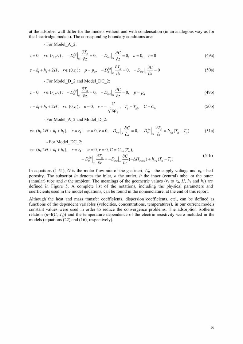
Condensation flux and condensation rate The condensation flux is calculated using equation (52). It is a function of both time and axial position in the adsorber. The time profiles of the condensation flux are shown in Figure 38, and the axial profiles in Figure 39.

These figures show that condensation starts at t=24 s and the condensation flux is maximal at approximately t=80s. At t=200s, when the power is switched of, the condensation is still not completely finished. At the beginning of the process the condensation flux increases from the bottom to the top of the adsorber, but with time the axial profile changes and the condensation is most intensive near the bottom of the adsorber.

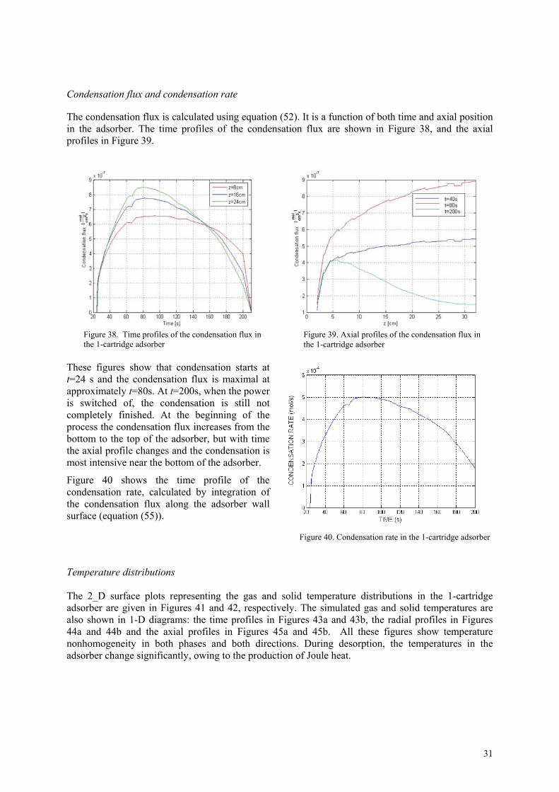
Figure 40 shows the time profile of the condensation rate, calculated by integration of the condensation flux along the adsorber wall surface (equation (55)). Temperature distributions The 2_D surface plots representing the gas and solid temperature distributions in the 1-cartridge adsorber are given in Figures 41 and 42, respectively. The simulated gas and solid temperatures are also shown in 1-D diagrams: the time profiles in Figures 43a and 43b, the radial profiles in Figures 44a and 44b and the axial profiles in Figures 45a and 45b. All these figures show temperature nonhomogeneity in both phases and both directions. During desorption, the temperatures in the adsorber change significantly, owing to the production of Joule heat.

Figure 38. Time profiles of the condensation flux inthe 1-cartridge adsorber

Figure 39. Axial profiles of the condensation flux in the 1-cartridge adsorber

Figure 40. Condensation rate in the 1-cartridge adsorber

32

(a) (b) (c)

Figure 41. Gas temperature distribution during desorption in the 1-cartridge adsorber: (a) t=24s, (b) t=80s and (c) t=200s

(a) (b) (c)

Figure 42. Solid temperature distribution during desorption in the 1-cartridge adsorber: (a) t=24s, (b) t=80s and (c) t=200s

33

Figure 43. Time profiles of the temperatures during desorption in the 1-cartridge adsorber, at z=16cm: (a) gas phase; (b) solid phase

(a) (b)

Figure 44. Radial profiles of the temperatures during desorption in the 1-cartridge adsorber, at z=16cm: (a) gas phase; (b) solid phase

(a) (b)

Figure 45. Axial profiles of the temperatures during desorption in the 1-cartridge adsorber, at r=1.25 cm: (a) gas phase; (b) solid phase

(a) (b)

34

Distribution of the electric resistivity of the ACFC adsorbent bed The electric resistivity of the ACFC is temperature dependent (decreases with the increase of temperature). As the temperature in the adsorbent bed varies considerably both in time and space, so does the electric resistivity. This dependence is shown in Figure 46 (in the form of a 2-D surface plot) and Figures 47, 48 and 49 (1-D diagrams showing time, radial and axial distributions, respectively).

The electric power transformed into Joule heat also changes, as a consequence of the change of the electric resistance. For constant voltage supply, the electric power increases with time, as shown in Figure 50. The electric power is calculated using equation (55).

Figure 47. Time profiles of the electric resistivity during desorption in the 1-cartridge adsorber, at z=16cm

(a) (b) (c)

Figure 46. The electric resistivity of the ACFC adsorbent distribution in the 1-cartridge adsorber: (a) t=24s, (b) t=80s and(c) t=200s

Figure 48. Radial profiles of the electric resistivity during desorption in the 1-cartridge adsorber, at z=16cm

35

4.1.3. TSA process in the 1-cartridge adsorber

The complete TSA process was simulated by using the integral Matlab/Femlab model presented in Figure 14. These simulations take long times, so they were limited to the first three cycles. The simulation results presented here were obtained for Tsw=463.15 K and Cbreak=0.5 Cin. All other simulation parameters are the same as in the simulations of adsorption and desorption. The time and space distributions of the velocity, concentrations and temperatures in the system during the adsorption and desorption half-cycles are very similar to the results presented in Sections 4.1.1 and 4.1.2, so they will not be given here. Instead, we are presenting the change of the outlet concentration from the adsorber during the first 3 cycles in Figure 51, the maximal temperature in the adsorbent bed in Figure 52 and the condensation rate in Figure 53. These figures show that the quasi-steady state is practically achieved after the second cycle.

Figure 50. Electric power supply during desorption in the 1-cartridge adsorber

Figure 51. The outlet concentration during TSA in the 1-cartridge adsorber (3 cycles)

Figure 49. Axial profiles of the electric resistivity in the 1-cartridge adsorber, for t=80 s

Figure 52. The maximal adsorbent temperature during TSA in the 1-cartridge adsorber (3 cycles) Figure 53. The condensation rate during TSA in the 1-

cartridge adsorber (3 cycles)

36

In Figure 53 an enlarged segment, showing the desorption step during the second cycle, is also given. From this segment, it can be seen that at the end of the desorption step, the condensation hasn’t been finished.

4.2. Simulation results for the 2-cartridges adsorber

4.2.1. Adsorption in the 2-cartridges adsorber

Owing to larger amount of adsorbent, the time needed to complete the adsorption process in the 2-cartridges adsorber is much longer than for the 1-cartridge adsorber. For that reason, these simulations were run for 11000 s or ~ 3 hours. The results presented here were obtained for the same inlet concentration and flow-rate as for the 1-cartridge adsorber (0.001 mol/mol and 0.1 mol/s).

Velocity distribution

The velocity field in the 2-cartridges adsorber is presented in Figures 54-57. In Figure 54, the velocity distribution at the end of adsorption (at t=110000 s) is shown in the form of a 2-D surface plot, together with a vector representation of the velocity. The velocity distribution is also presented in 1-D diagrams: the time profiles at the middle cross-sections of both cartridges (z=16 cm and z=42 cm) and 4 radial positions in Figure 55, the radial profiles at z=16 cm and z=42 cm in Figure 56 and the axial profiles in several radial positions in Figure 57.

Figure 54. Velocity distribution of the gas phase during adsorption in the 2-cartridge adsorber for t=11000s

Figure 55. Time profiles of the gas velocity during adsorption in the 2-cartridge adsorber at z=16 cm (solid lines) and z=49 cm (dashed lines)

37


The 2-D surface plots of the gas and solid concentration distributions during adsorption in the 2-cartridges adsorber are given in Figures 58 and 59, respectively. The concentrations at three distinct moments (t=100, 400 and 11000 s) are shown. For t=11000 s the gas concentration in the adsorber is uniform and equal to the feed concentration (0.001 mol/mol), i.e., the adsorption process is finished. At early stages of adsorption, the concentrations in the adsorber are nonuniform.

The concentration profiles are also given in 1-D diagrams: the time profiles at z=16 cm in Figure 60, the radial profiles at z=16 cm in Figure 61 and the axial profiles for t=200 s in Figure 62. Figures 60a, 61a and 62a correspond to the gas phase and Figures 60b, 61b and 62b to the solid phase.

(a) (b) (c)

Figure 60. Gas concentration distribution during adsorption in the 2-cartridges adsorber: (a) t=100s, (b) t=400s and (c) t=11000s

Figure 56. Radial profiles of the gas velocity during adsorption in the 2-cartridge adsorber for t=11000 s

Figure 57. Axial profiles of the gas velocity during adsorption in the 2-cartridge adsorber at r=1.25 cm

38

(a) (b) (c)

Figure 61. Solid concentration distribution during adsorption in the 2-cartridges adsorber: (a) t=100s, (b) t=400s and(c) t=11000s

Figure 62. Time profiles of the concentrations in the 2-cartridges adsorber, at z=16cm (solid lines) and at z=49cm (dashed lines): (a) gas phase; (b) solid phase

(a) (b)

Figure 63. Radial profiles of the concentrations during adsorption in the 2-cartridges adsorber, at z=16cm (solid lines) and z=49cm (dashed lines): (a) gas phase; (b) solid phase

(a) (b)

39

Considerable differences between the concentrations in the two cartridges can be observed. These differences diminish in time, as both cartridges become nearly saturated. Temperature distributions The gas and solid temperature distributions during adsorption in the 2-cartridges adsorber are given in Figures 65 and 66, respectively, in the form of 2-D surface plots. The simulated temperatures are also shown in 1-D diagrams: the time profiles in Figures 67a and 67b, the radial profiles in Figures 68a and 68b and the axial profiles in Figures 69a and 69b. All these figures show temperature nonhomogeneity in both phases. The maximal temperature rise during adsorption is less than 4 oC, for the 2-cartridges adsorber. The highest temperature is observed after approximately 400 s from the start of adsorption.

(a) (b) (c)

Figure 65. Gas temperature distribution during adsorption in the 2-cartridges adsorber: (a) t=100s, (b) t=400s and (c) t=11000s

Figure 64. Axial profiles of the concentrations during adsorption in the 2-cartridges adsorber, for t=200 s: (a) gas phase; (b) solid phase

(a) (b)

40

(a) (b) (c)

Figure 66. Solid temperature distribution during adsorption in the 2-cartridges adsorber: (a) t=100s, (b) t=400s and (c) t=11000s

(a) (b)

Figure 67. Time profiles of the temperatures during adsorption in the 2-cartridges adsorber, at z=16cm (solid lines) and z=49cm (dashed lines): (a) gas phase; (b) solid phase

(a) (b)

Figure 68. Radial profiles of the temperatures during adsorption in the 2-cartridges adsorber, at z=16cm (solid lines) and z=49cm (dashed lines): (a) gas phase; (b) solid phase

41

Large differences between the temperature profiles in the two cartridges can also be observed. 4.2.2. Desorption in the 2-cartridges adsorber Again, the complete desorption step is simulated, by using a combination of Model_D_2 and Model_DC_2. The results presented here were obtained for initial concentration in the solid phase 0.00465 mol/g, electric voltage 11 V and inert gas flow-rate 0.01 mol/s per cartridge (0.002 mol/s in total). The time scale used for this simulation is the same as for the 1-cartridge adsorber: 0 to 200s. Velocity distribution

The velocity distribution at the end of desorption (at t=200 s) is shown in Figure 70, in the form of a 2-D surface plot, together with vector representation of the velocity. The velocity distribution is also presented in 1-D diagrams: the time profiles in Figure 71, the radial profiles in Figure 72 and the axial profiles in Figure 73. Some (not significant) change of the velocity profile in time is present, as a result of the change of the gas temperature.

Figure 70. Velocity distribution of the gas phase during desorption in the 2-cartridge adsorber at t=200 s

Figure 71. Time profiles of the gas velocity during desorption in the 2-cartridge adsorber, at z=16cm (solid lines) and at z=49cm (dashed lines)

Figure 69. Axial profiles of the temperatures during adsorption in the 2-cartridges adsorber, for t=200 s: (a) gas phase; (b) solid phase

(a) (b)

42


The gas and solid concentration distributions during desorption in the 2-cartridges adsorber, presented in the form of 2-D surface plots, are given in Figures 74 and 75, respectively. The concentrations at three distinct moments (t=30, 90 and 200 s) are shown (t=30 s is the moment when condensation starts, i.e. when the program switches from Model_D_2 to Model_DC_2). The concentration profiles are also shown in 1-D diagrams: the time profiles in Figure 76, the radial profiles in Figure 77 and the axial profiles in Figure 78. Figures 76a to 78a correspond to the gas phase and Figures 76b to 77b to the solid phase.

Figure 74. Gas concentration distribution during desorption in the 2-cartridges adsorber: (a) t=30s, (b) t=90s and (c)

t=200s Contrary to the case of adsorption, for desorption the concentration distributions in the two cartridges are similar. This is a result of the symmetrical inlet streams in the two cartridges.

(a) (c) (b)

Figure 72. Radial profiles of the gas velocity during desorption in the 2-cartridge adsorber, for t=200 s

Figure 73. Axial profiles of the gas velocity during desorption in the 2-cartridge adsorber, for t= 200 s

43

Figure 75. Solid concentration distribution during desorption in the 2-cartridges adsorber: (a) t=30s, (b) t=90s and (c) t=200s

(a) (b) (c)

Figure 76. Time profiles of the concentrations during desorption in the 2-cartridge adsorber, at z=16cm (solid lines) and at z=49cm (dashed lines): (a) gas phase; (b) solid phase

(b) (a)

Figure 77. Radial profiles of the concentrations during desorption in the 2-cartridge adsorber, at z=16cm (solid lines) and at z=49cm (dashed lines): (a) gas phase; (b) solid phase

(a) (b)

44

Condensation flux and condensation rate The condensation flux, calculated by using equation (52) is shown in Figure 79 (the time profiles) and Figure 80 (the axial profiles).

These figures show that condensation starts at t=30 s and the condensation flux is maximal at approximately t=60s. At t=200s, when the power is switched of, the condensation is still not completely finished. At the beginning of the process the condensation flux increases from the adsorber ends towards its middle, with a sharp minimum at the middle cross-section, between the two-cartridges.

Figure 81 shows the time profile of the condensation rate, calculated by integration of the condensation flux along the adsorber wall surface.

Figure 80. Axial profiles of the condensation flux in the 2-cartridges adsorber

Figure 78. Axial profiles of the concentrations during desorption in the 2-cartridge adsorber, for t=80 s: (a) gas phase; (b) solid phase

(a) (b)

Figure 79. Time profiles of the condensation flux in the 2-cartridge adsorber

Figure 81. Condensation rate in the 2-cartridges adsorber

45

Temperature distributions The gas and solid temperature distributions in the 2-cartridges adsorber in which desorption is taking place are again presented in the form of 2-D surface plots (Figures 82 and 83) and in 1-D plots: the time profiles in Figures 84a and 84b, the radial profiles in Figures 85a and 85b and the axial profiles in Figures 86a and 86b. All these figures show temperature nonhomogeneity in both phases and large temperature changes during desorption. Similarity between the temperature distributions in the two cartridges can easily be observed.

Figure 82. Gas temperature distribution during desorption in the 2-cartridges adsorber: (a) t=30s, (b) t=90s and (c) t=200s

Figure 83. Solid temperature distribution during desorption in the 2-cartridges adsorber: (a) t=30s, (b) t=90s and (c) t=200s

(a) (c) (b)

(a) (c) (b)

46

Figure 84. Time profiles of the temperatures during desorption in the 2-cartridges adsorber, at z=16cm (solid lines) and z=49cm (dashed lines): (a) gas phase; (b) solid phase

(a) (b)

Figure 85. Radial profiles of the temperatures during desorption in the 2-cartridges adsorber, at z=16cm (solid lines) and z=49cm (dashed lines): (a) gas phase; (b) solid phase

(a) (b)

Figure 86. Axial profiles of the temperatures during desorption in the 2-cartridges adsorber, for t=80 s (a) gas phase; (b) solid phase

(a) (b)

47

Distribution of the electric resistivity of the ACFC adsorbent bed The distribution of the electric resistivity in the 2-cartridges adsorber is shown in Figure 87 (in the form of 2-D surface plot) and in Figures 88, 89 and 90 (the 1-D diagrams showing the time, radial and axial distributions, respectively).

Figure 87. Distribution of the electric resistivity of the ACFC adsorbent in the 2-cartridges adsorber: (a) t=30s, (b) t=90s and (c) t=200s

The time dependence of the electric power is shown in Figure 91.

(a) (b) (c)

Figure 88. Time profiles of the electric resistivity in the 2-cartridges adsorber, at z=16cm (solid lines) and at z=49cm (dashed lines)

Figure 89. Radial profiles of the electric resistivity in the 2-cartridges adsorber, at z=16cm (solid lines) and z=49cm (dashed lines)

48

4.2.3. TSA process in the 2-cartridges adsorber

The simulation results presented here were obtained for Tsw=463.15 K and Cbreak=0.5 Cin. All other simulation parameters are the same as in the simulations of adsorption and desorption. The change of the outlet concentration from the adsorber during the first 3 cycles in is shown in Figure 92, the maximal temperature in the adsorbent beds in Figure 93 and the condensation rate in Figure 94. The quasi-steady state is practically achieved after the second cycle.

It should be noticed that the TSA cycle in the 2-cartridges adsorber lasts considerably longer that in the 1-cartridge adsorber. This is primarily a result of a much longer adsorption half-cycle.

Figure 90. Axial profiles of the electric resistivity in the 2-cartridges adsorber, for t=80 s

Figure 92. Time profiles of the outlet concentration in the 2-cartridges adsorber, for 3 cycles

Figure 93. Maximal adsorbent temperature in the 2-cartridges adsorber for 3 cycles

Figure 94. Condensation rate in the 2-cartridges adsorber for 3 cycles

Figure 91. Used electric energy during desorption in the 2-cartridges adsorber

49

5. Analysis of the influence of process parameters and optimization of the TSA process

In order to analyze the results of the TSA processes, some performance criteria should be defined, as measures of the process quality. We define the following criteria:

• Adsorption time (duration of the adsorption half-cycle), τA

• Desorption time (duration of the desorption half-cycle), τD

• Average outlet concentration during adsorption, <Cout>A

• Average outlet concentration during desorption, <Cout>D

• Separation factor defined as the ratio of the average outlet concentrations during adsorption and desorption, αs=<Cout>D/ <Cout>A

• Purification factor, defined as the ratio of the outlet and inlet concentrations during adsorption, αp= <Cout>A/Cin,A

• The total amount of condensed liquid per cycle, Lcond

• Used electric energy per cycle, Qel

• Used energy per mol of condensate, Qel/Lcond

In principle, the following can be considered as favourable:

- Long adsorption time

- Short desorption times

- Low outlet concentration during adsorption

- High outlet concentrations during desorption

- High separation factor

- Low purification factor

- Large amount of condensed liquid per cycle

- Low energy spent per cycle

- Low energy spent per mole of condensate.

In this section, we will analyze how these criteria are influenced by the change of some input parameters of the TSA process. The influence of the following parameters was chosen for analysis:

- The maximal adsorbent temperature at which the TSA cycle is switched from desorption to adsorption – the switch temperature Tsw;

- The breakthrough concentration for which the TSA cycle is switched from adsorption to desorption, Cbreak;

- The electrical voltage used during desorption U0;

- The inert flow-rate during the adsorption part of the cycle GA;

- The inert flow-rate during the desorption part of the cycle GD.

The analysis was performed by changing one of these five parameters at a time and keeping all the others constant. The “fixed” parameters have the same values as in the simulations presented in the previous section. For each combination of parameters the 9 criteria defined previously were calculated. The results are presented in tabular form.

The results presented in this section correspond to the second cycles of the simulated TSA processes.

50

The results obtained for the 1-cartridge adsorber are presented first. 5.1. Analysis for the 1-cartridge adsorber In Table 3 we present the performance criteria chosen for analysis obtained for three different switch temperatures .

Table 3. Analysis of the influence of the switch temperature Tsw, for the 1-cartridge adsorber

Switch temperature Tsw [K] Criteria 433.15 463.15 493.15

<Cout>D [mol/mol] 0.00853 0.00879 0.00895 <Cout>A [mol/mol] 2.65e-04 2.00e-04 1.84e-04

αs=<Cout>D /<Cout>A 32.189 43.950 48.641 αp=<Cout>A /Cin,A 0.265 0.200 0.184

Lcond [mol] 0.0400 0.0499 0.0557 Qel [KJ] 13.363 16.735 19.593

Qel / Lcond [KJ/mol] 334.07 335.37 351.76 τD [s] 130 158 180 τA [s] 2370 2440 2600

These results show that the following criteria increase with increasing the switch temperature: the adsorption and desorption times, the outlet concentration during desorption and the separation factor, the condensed liquid and the used energy per cycle. On the other hand, the outlet concentration during adsorption and the purification factor decrease with increasing Tsw. The energy consumption per mole of condensate is nearly constant. It could be concluded that the increase of the switch temperature is favorable from the point of view of separation and purification of the feed stream, as well as regeneration of the adsorbed vapor, but unfavorable from the point of view of energy consumption. It should also be remembered that the switch temperature is often limited by the temperature of degradation of some thermally unstable materials used in the process.

In Table 4 we show the influence of the breakthrough concentration, i.e., the outlet gas concentration for which the TSA process is switched from adsorption to sorption. Table 4. Analysis of the influence of the breakthrough concentration Cbreak, for the 1-cartridge adsorber

Breakthrough concentration Cbreak [mol/mol] Criteria 2.5e-4 (25% Cin) 3.5e-4 (35% Cin) 5.0e-4 (50% Cin)



Lcond [mol] 0.0397 0.0437 0.0499 Qel [KJ] 15.268 15.717 16.735


The results given in Table 4 show that the increase of the breakthrough concentration results in longer adsorption and desorption times, higher outlet concentrations during both adsorption and desorption,

51

lower separation and higher purification factors, larger amounts of condensed liquid and energy spent per cycle, but lower energy consumption per mole of condensed liquid. Table 5 shows the criterial parameters corresponding to simulations obtained with 3 different values of the supply voltage during desorption.

Table 5. Analysis of the influence of the voltage used for desorption, U0, for the 1-cartridge adsorber

Supply voltage U0 [V] Criteria 10 11 12



Lcond [mol] 0.0500 0.0499 0.0510 Qel [KJ] 19.626 16.735 15.433


When the supply voltage during desorption increases, slightly shorter adsorption and considerably shorter desorption times are obtained. The outlet concentrations during adsorption and desorption both increase with the increase of U0, but only slightly, as well as the purification factor. The separation factor decreases somewhat, and the used energy per cycle and per mole of condensate considerably. The amount of condensed liquid per cycle doesn’t change considerably. Tables 6 shows the influence of the flow-rate during adsorption, GA, and Table 7 of the flow-rate during desorption, GD, on the criteria chosen for comparison. For the chosen range of flow-rates and for the parameters used for simulation, these influences are not significant. Table 6. Analysis of the influence of the flow-rate during adsorption GA, for the 1-cartridge adsorber

Flow-rate during adsorption GA [mol/s] Criteria 0.08 0.09 0.10

<Cout>D [mol/mol] 0.00878 0.0088 0.00879 <Cout>A [mol/mol] 2.02E-04 2.01E-04 2.00e-04


Lcond [mol] 0.0502 0.0506 0.0499 Qel [KJ] 16.737 16.842 16.735


52

Table 7. Analysis of the influence of the flow-rate during desorption GD, for the 1-cartridge adsorber

Flow-rate during desorption GD [mol/s] Criteria 0.01 0.02 0.03



Lcond [mol] 0.0499 0.0528 0.0526 Qel [KJ] 16.735 17.471 17.900


5.2. Analysis for the 2-cartridges adsorber

As our analysis for the 1-cartridge adsorber showed that the flow-rates don’t influence the TSA process much, only three input parameters were varied for the 2-cartridges adsorber: the switch temperature, the breakthrough concentration and the electric voltage. Their influence on the analyzed performance criteria of the TSA process is shown in Tables 8, 9 and 10, respectively.

Table 8. Analysis of the influence of the switch temperature Tsw, for the 2-cartridges adsorber

Switch temperature Tsw [K] Criteria 433.15 463.15 485.28

<Cout>D [mol/mol] 0.00921 0.00933 0.00936 <Cout>A [mol/mol] 2.78E-04 2.30E-04 2.22E-04


Lcond [mol] 0.114 0.1270 0.131 Qel [KJ] 34.648 41.890 44.665


Table 9. Analysis of the influence of the breakthrough concentration Cbreak, for the 2-cartridges adsorber

Breakthrough concentration Cbreak [mol/mol] Criteria 2.5e-4 (25% Cin) 3.5e-4 (35% Cin) 5.0e-4 (50% Cin)



Lcond [mol] 0.0879 0.1030 0.1270 Qel [KJ] 35.986 37.531 41.890


53

Table 10. Analysis of the influence of the voltage supply U0, for the 2-cartridges adsorber

Voltage supply U0 [V] Criteria 10 11 12



Lcond [mol] 0.1197 0.1270 0.1235 Qel [KJ] 45.837 41.890 35.899


Similar conclusions as for the 1-cartridge adsorber can be withdrawn.

Comparison of the results obtained for the 1-cartridge and 2-cartridges adsorbers shows that the adsorption times are more than double and the desorption times about 50% longer for the 2-cartridges adsorber. The separation and the purification factors are similar for both adsorbers. On the other hand, the amount of condensed liquid and the used energy per cycle for the 2-cartridges adsorber are more than double than for the 1-cartridge adsorber. Nevertheless, the values of the energy spent per mole of condensate are similar for both adsorber types.

5.3. Discussion of the results and some recommendations for choosing the optimal input parameters The inspection of the results listed in Tables 3-10 shows that unexpectedly low values of the amount of condensed liquid per cycle are obtained. The reason for that could be in the fact that the desorption step in our model is ended when the predefined switch temperature is reached, while the condensation process is still not finished, as can be seen from Figure 53 (similar picture is obtained for the 2-cartridges adsorber). After that moment, the simulation switches to the adsorption model, which doesn’t assume condensation. In order to resolve this imprecision, an additional model segment should be incorporated in the integral TSA model, for an additional step of the TSA process of desorption with in-vessel condensation, but without electrical heating. We expect that such a model would predict larger, more realistic amounts of condensate per cycle, especially for the cases with short desorption times. The spent energy per cycle would remain unchanged, so we expect that much lower values of the energy consumption per mole of condensate would be obtained.

Regarding the influence of the input parameters on the TSA performance criteria, there is no ideal solution, i.e. all input parameters influence some of the criteria in a favorable and some in an unfavorable way. For that reason, the recommendations for choosing optimal input parameters depend on the priorities of the performance criteria. Here are some examples:

- If purification of the gas stream is the main priority, lower values of the breakthrough concentration should be used. Higher switch temperature and lower supply voltage, also result with more efficient purification, to some extent.

- If regeneration of the vapor in the liquid form is the priority of the process, one should use high switch temperature, large breakthrough concentration and high voltage.

- If energy efficiency of the process is the primary goal, low switch temperature, large breakthrough concentration and high voltage should be used.

54

6. Conclusions and possibilities for model improvement

In this phase of the project we have developed two complex models for simulation of integral TSA cycles in adsorbers with one or two annular, radial-flow, cartridge-type adsorption beds. Each model was built of three segments, corresponding to three steps of the TSA process: adsorption, electrothermal desorption and electrothermal desorption with in-vessel condensation. The individual segments were built using Femlab software, while Femlab with Matlab was used for building the integral TSA models.

The models were successfully used for simulation of separate stages and complete TSA cycles in the 1-cartridge and 2-cartridges adsorbers and for analysis of the influence of the main input parameters on the system performance. Some basic recommendations regarding the choice of the input parameters of the TSA process were given based on it, in order to show that the developed models can be used for optimization.

The models were developed and run on Pentium 4 PCs, with 1 GB RAM memory. During their development, convergence problems occurred frequently. Regarding convergence, the models are pretty sensitive on the choice of the model parameters. The computer times needed for simulations were generally long, but differed from case to case. In principle, the computer times needed to solve the 2-cartridges model were much longer than for the 1-cartridge model.

In spite of the great complexity of the developed models, there are still some possibilities for their upgrading in order to make them more realistic. Some of them would be:

- Adding a model segment defining the end of the desorption half-cycle without heating, between switching the power off and the end of condensation.

- Adding relations for calculation of some physical and transport parameters and coefficients as functions of the temperatures, concentrations and velocities in the system, instead of using constant values.

- Adding a model for the heat balance of the adsorber wall.

55

Nomenclature

a (m2/m3) - Specific surface area

b (K-1) - Temperature coefficient of the bed electrical resistivity

C (mol/mol) - Adsorbate concentration in the gas phase

C*(mol/mol) - Adsorbate concentration in the gas phase in equilibrium with the solid phase

Cbreak (mol/mol) - Breakthrough concentration

Csat (mol/mol) - Saturation concentration

cpg (J/mol/K) - Specific heat capacity of the inert gas

cpl (J/mol/K) - Specific heat capacity of liquid adsorbate

cps (J/g/K) - Heat capacity of the solid phase

cpv (J/mol/K) - Specific heat capacity of gaseous adsorbate

Dmr (mol/cm/s) - Radial mass transfer dispersion coefficient

Dmz (mol/cm/s) - Axial mass transfer dispersion coefficient

Dthg (W/K/cm) - Heat diffusivity of the gas phase

Dths (W/K/cm) - Heat diffusivity of the solid phase

E (J/mol) - Adsorption energy of the adsorbate (D-R eq.)

g (cm/s2) - Gravitation constant

G (mol/s) - Flow rate of the inert gas

H (cm) - Bed axial dimension (Fig. 5)

h1 (cm) - Adsorber dimension (Fig. 5)

h2 (cm) - Adsorber dimension (Fig. 5)

hb (J/cm2/K) - Solid to gas heat transfer coefficient

hs1 (J/cm2/K) - Heat transfer coefficient from the solid phase to the gas phase in the central tube(s)

hs2 (J/cm2/K) - Heat transfer coefficient from the solid phase to the gas phase in the annular tube

hwg (J/cm2/K) - Gas to ambient heat transfer coefficient (heat losses)

J (A/cm2) - Current density

Jcond (mol/cm2/s) - Condensation flux

k (cm2) - Asorbent bed permeability

km (mol/cm2/s) - Mass transfer coefficient in the adsorbent bed

km1 (mol/cm2/s) - Mass transfer coefficient between the adsorbent bed and the gas in the central tube

km2 (mol/cm2/s) - Mass transfer coefficient between the adsorbent bed and the gas in the annular tube

condL& (mol/s) - Flow-rate of the condensed liquid

Lcond (mol) - Total amount of the condensed liquid

p (Pa) - Gas pressure

pA (Pa) - Adsorbate partial pressure

56

pc (Pa) - Critical pressure

p0 (Pa) - Adsorbate saturation pressure

elQ& (W) - Rate of heat generation (equal to electric power)

Qel (J) - Heat generation (equal to electric energy)

q (mol/g) - Adsorbate concentration in the solid phase

Rg (J/mol/K) - Gas constant

r (cm) - Radial dimension

r1 (cm) - Adsorber dimension (Fig. 5)




Ta (K) - Ambient temperature

Tg (K) - Gas phase temperature

Tc (K) - Critical temperature

TR (K) - Referent temperature

Ts (K) - Solid phase temperature

Tsw (K) - Switch temperature (from desorption to adsorption)

Tw (K) - Wall temperature

t (s) - Time

U (V) - Electric potential

U0 (V) - Supply voltage

u (cm/s) - Radial superficial gas velocity

VPA, VPB, VPC, VPD - Wagner constants

v (cm/s) - Axial superficial gas velocity

W (cm3/g) - Adsorbate volume per 1 g of the adsorbent mass

W0 (cm3/g) - Total volume of micropores (D-R equation)

Greek letters:

αp - Purification factor

αr - Regeneration factor

αs - Separation factor

∆Hads (J/mol) - Heat of adsorption

∆Hcond (J/mol) - Heat of condensation

εb - Bed porosity

µ (Pa/s) - Dynamic viscosity

ρ (Ωcm) - Electric resistivity

ρ0 (Ωcm) - Electric resistivity at referent temperature TR

57

ρg (mol/cm3) - Gas phase density

ρb (g/cm3) - Adsorbent bed density

ρA (g/cm3) - Adsorbate density

τ (s) - “Half” cycle

Subscripts:

A - adsorption

b - bed

D - desorption

g - gas

in - inlet

out - outlet

p - previous (initial)

r - radial

s - solid phase

it - inner (central) tube

ot - outer (annular) tube

z - axial

Special characters:

< > - time average value

58

References

1. Fabuss, B.M. and W.H. Dubois, “Carbon Adsorption-Electrodesorption Process”, 63rd Annual Meeting of the Air Pollution Control Association, St. Louis, Missouri (1970)

2. Petkovska, M. et al, “Temperature-swing gas separation with electrothermal desorption step”, Sep. Sci. Technol., 26, 425-444 (1991)

3. Petkovska, M.; Mitrović, M., “Microscopic modelling of electrothermal desorption”, Chem. Eng. J. Biochem. Eng. J, 53, 157-165 (1994a)

4. Petkovska M. and Mitrović M., “One-dimensional, non-adiabatic, microscopic model of electrothermal desorption process dynamics”, Chem. Eng. Res .Des., 72, 713-722 (1994b)

5. Sullivan P., “Organic vapor recovery using activated carbon fiber cloth and electrothermal desorption”, Ph.D. Thesis, University of Illinois at Urbana-Champaign (2003)

6. Bathen, D., “Gasphasen - Adsorption in der Umwelttechnik - Stand der Technik und Perspektiven”, Chemie Ingenieur Technik, 74, 209-216 (2002)

7. Subrenat A. and Le Cloirec P, “Industrial application of adsorption onto activated carbon cloths and electro-thermal regeneration”, J. Environ. Eng., 130, 249-257 (2004)

8. Sullivan P. et al, “Capture of Organic Vapors Using Adsorption and Electrothermal Regeneration”, J. Environ. Eng., 130, 258-267 (2004)

9. Rood M. et al, “Selective sorption and desorption of gases with electrically heated activated carbon fiber cloth element” US Patent No. 6,346,936 B1(2002)

10. Petkovska M., “Rigorous Mathematical Modeling of Adsorption System with Electrothermal Regeneration of the Used Adsorbent”, Final Performance Report for Project No. FA8655-03-1-3010, Year 1 (2004)

Documents

RIGOROUS MATHEMATICAL MODELING OF ADSORPTION …