Rikvold Presentation

Kinetic Monte Simulation:Comparison with Cyclic-Voltammetry

Aaron Hastings

2

• Lattice-Gas Model• Kinetic Monte Carlo• Metropolis-Hastings Algorithm

• Cyclic Voltammetry

Overview:

3

• Governing Hamiltonian • (used to calculate energy

• => occupation variable• =1 (occupied)• =0 (unoccupied)

Lattice-Gas Model:

4

• Interaction Constants

• Electrochemical Potential

Lattice-Gas Model:

5

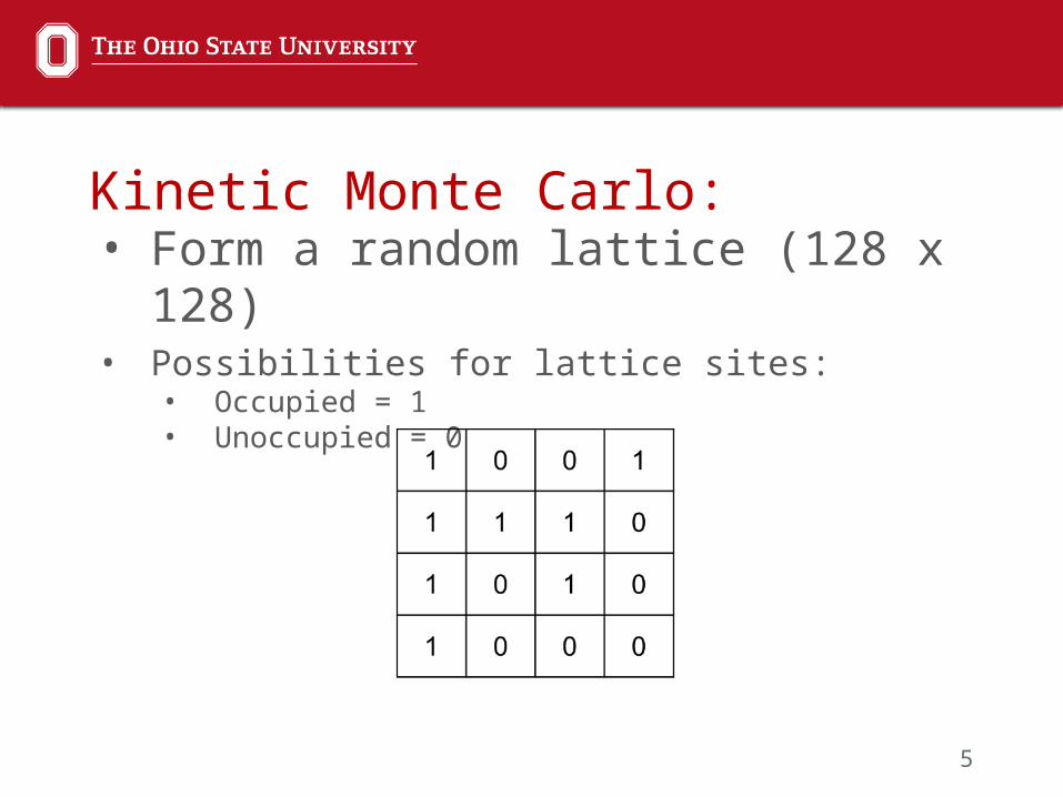
• Form a random lattice (128 x 128)• Possibilities for lattice sites:

• Occupied = 1• Unoccupied = 0

Kinetic Monte Carlo:

6

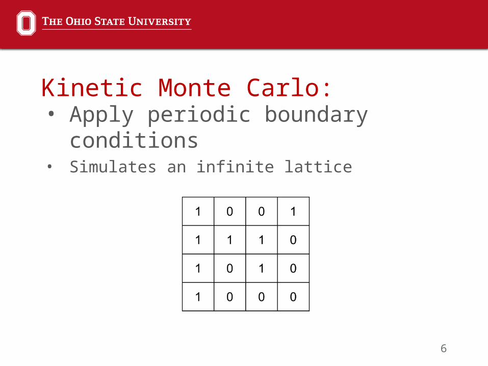
• Apply periodic boundary conditions• Simulates an infinite lattice


7

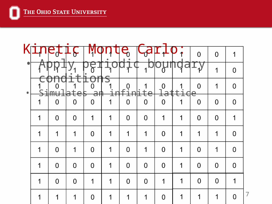
• Apply periodic boundary conditions• Simulates an infinite lattice


8

• Choose a random lattice site, i• Possibilities for moves at i:

• If occupied (=1)• Adsorption• If unoccupied (=0)• List of nine options


9

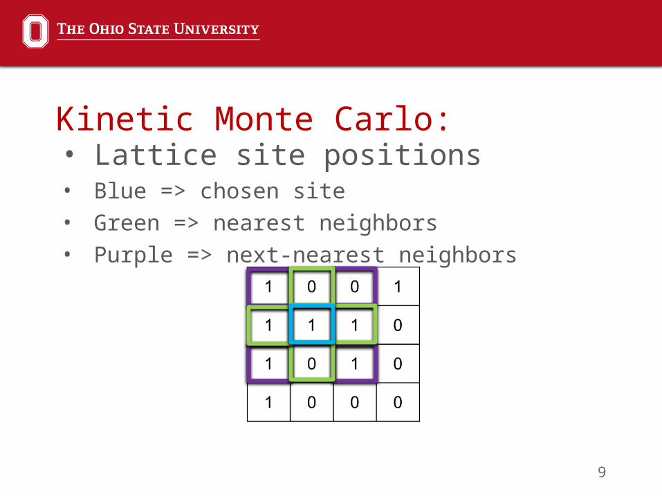
• Lattice site positions• Blue => chosen site• Green => nearest neighbors• Purple => next-nearest neighbors


10

• Site i is unoccupied:• If nearest neighbor sites are unoccupied:• Adsorption to the site is attempted


11

• Site i is occupied:• If nearest neighbor sites are occupied:• Desorption occurs with 100% probability

• Otherwise, check if next-nearest neighbor sites are unoccupied:

• Propose a diffusion to:• Any one of the 4 nearest neighbors• Any one of the 4 next-nearest neighbors


12

• Form a weighted list of probabilities:

• => “Bare” barrier associated with process • β => 1/(kbT)• => Energy change for the move


13

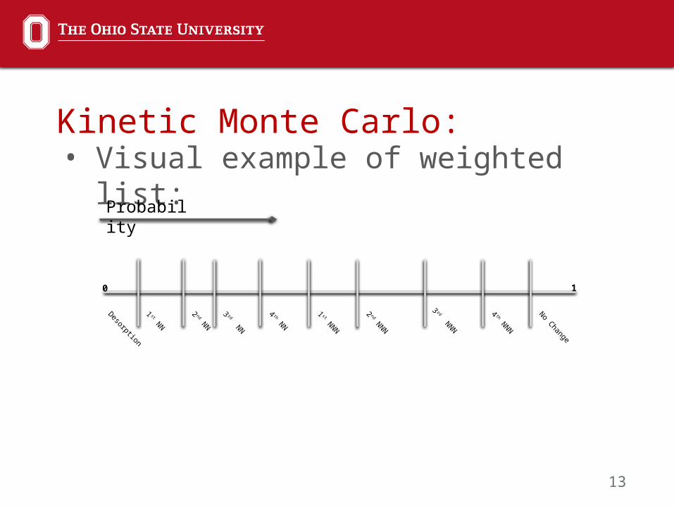
• Visual example of weighted list:Kinetic Monte Carlo:

Desorption

1 st NN

2 nd NN

3 rd NN

4 th NN

1 st NNN

4 th NNN

2 nd NNN

3 rd NNN

No Change

0 1

Probability

14

• Attempt a move:• Generate a random number between (0,1):• Check where it falls on the weighted list:

• Accept the move


15

• Repeat for potential, µ:• -200meV ≤ µ ≤ 600meV (increasing µ)• 600meV ≥ µ ≥ -200meV (decreasing µ)

• Total number of attempts:

• L => Lattice dimension • => Scan rate (3*10^-5 to 0.1meV/MCSS)


16

• Run eight simulations at each scan rate• Average the data• θ => Lattice Coverage

• Take a numerical derivative• Apply a Savitzky-Golay filter in MATLAB• dθ/dµ

Cyclic Voltammetry:

17

• Smoothed numerical derivative is proportional to current density, j:

• Differential adsorption capacitance per unit area:

Cyclic Voltammetry:

18

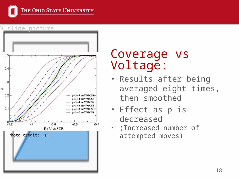
Coverage vs Voltage:• Results after being averaged

eight times, then smoothed• Effect as ρ is decreased• (Increased number of attempted

moves)

½ slide picture

Photo credit: [1]

19

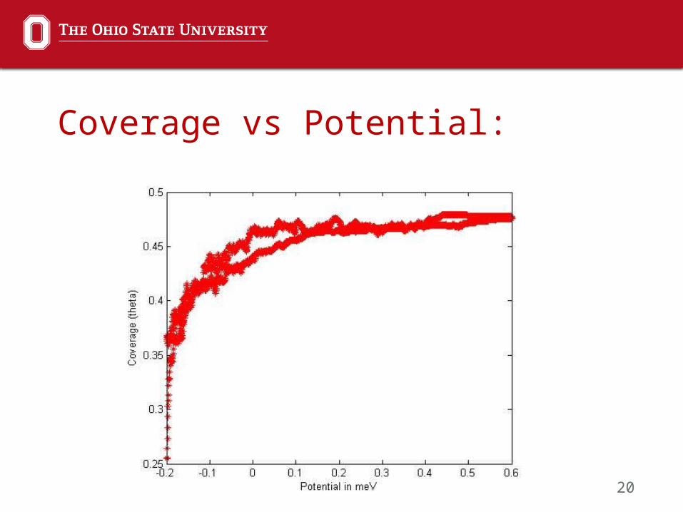
• Laptop trial:• 30 x 30 lattice with ρ = 0.5

• Witnessed similar trends• Supercomputer trial:• 64 x 64 lattice with ρ = 1*10-3

Coverage vs Voltage:

20

Coverage vs Potential:

21

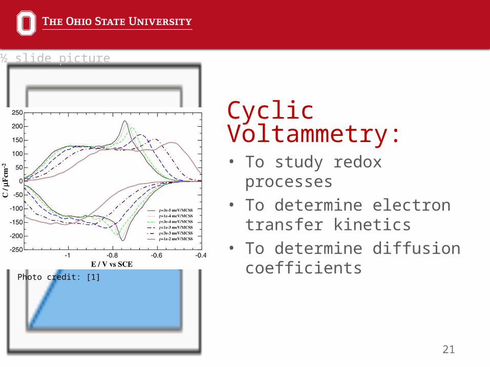
Cyclic Voltammetry:• To study redox processes• To determine electron transfer

kinetics• To determine diffusion

coefficients

½ slide picture

Photo credit: [1]

22

• Submitted a few trials to OSC• (Ohio Supercomputer Center)

• Need to further debug/optimize our code• Use DFT to establish parameters for

Uranium• (Density Functional Theory)

• Determine boundary conditions for Diffusion Equation at the surface

Future Plans:

23

1. Abou, Hamad I, P.A Rikvold, and G Brown. "Determination of the Basic Timescale in Kinetic Monte Carlo Simulations by

Comparison with Cyclic-Voltammetry Experiments." Surface Science. 572 (2004). Print.

2. Abou, Hamad I, Th Wandlowski, G Brown, and P.A Rikvold. "Electrosorption of Br and Cl on Ag(1 0 0): Experiments and Computer Simulations." Journal of Electroanalytical Chemistry. (2003): 554-555. Print.

References:

24

Thank you.

Any questions?

Documents

Rikvold Presentation