Embed Size (px)
Citation preview
Geology & GeosciencesKrishna et al., J Geol Geosci 2014, 3:3
http://dx.doi.org/10.4172/2329-6755.1000152
Open AccessResearch Article
Volume 3 • Issue 3 • 1000152J Geol GeosciISSN: 2329-6755 JGG, an open access journal
Tropical Indian Ocean Surface and Subsurface Temperature Fluctuations in a Climate Change ScenarioMuni Krishna K1*, Guiting Song2, Dennis Jack3 and Manjunatha BR4
1Department of Meteorology and Oceanography, Andhra University, Visakhapatnam, India2Department of Marine Science, Zhejiang Ocean University, China3Departamento de Astronomia Universidad de Guanajuato, Mexico4Department of Marine Geology, Mangalore University, Mangalagangotri, India
*Corresponding author: Muni Krishna K, Department of Meteorology and Oceanography, Andhra University, Visakhapatnam, India, Tel: 08912844633; E-mail: [email protected]
Received December 23, 2013; Accepted March 05, 2014; Published March 14, 2014
Citation: Krishna KM, Song G, Jack D, Manjunatha BR (2014) Tropical Indian Ocean Surface and Subsurface Temperature Fluctuations in a Climate Change Scenario. J Geol Geosci 3: 152. doi: 10.4172/2329-6755.1000152
Copyright: © 2014 Krishna KM, et al. This is an open-access article distributed under the terms of the Creative Commons Attribution License, which permits unrestricted use, distribution, and reproduction in any medium, provided the original author and source are credited.
Keywords: Sea surface temperature; Indian Ocean; Indian Ocean Dipole (IOD); El Nino Southern Oscillation (ENSO)
IntroductionThe oceans cover about 71% of the Earth’s surface and have an
average depth of 3.7 km. This adds up to a huge amount of water with a mass of about 1.3×10²¹ kg and a correspondingly enormous heat capacity, which is a 1000 times larger than that of the Earth’s atmosphere. Thus, the ocean acts as a large reservoir of heat that in turn drives the Earth’s climate system. The energy and mass exchanges between the ocean and the atmosphere take place at the interface boundary and, therefore, the study of air-sea interaction has great importance in understanding the dynamics of climate change. Among the oceans, the tropical ocean basins, encompassing the equatorial regions, have a special place in modulating the regional as well as the global climate. In recent decades, global oceans are warming up. This has been measured by several observations and models [1-5]. This global warming has been attributed mostly to human-induced greenhouse gases, which increase surface heat fluxes into the ocean [2,3,6,7]. Recently, Barnett et al. [7] examined how the surface warming penetrates down into the deeper oceans. They showed that the warming has a distinct vertical structure in the Indian and Pacific Oceans, with a large amplitude of warming above 100 m, cooling near 100-250 m, and a weaker warming around 250-700 m depth.
The Indian Ocean with its northern extent limited to the tropical belt experiences semi-annual wind forcing – the southwest and northeast monsoons. As a result of weak winds (<1-3 m/s), the equatorial thermocline is flat and deep. Such an annual-mean climatology - deep thermocline and absence of equatorial upwelling - limits the effect of thermocline depth variability on the sea surface temperature (SST), a key element to the Bjerknes feedback, leading to the fact that the Indian Ocean cannot develop its own inter-annual variability and thus has to follow the Pacific El Nino Southern Oscillation (ENSO) rather passively. The unique features of the Equatorial Indian Ocean (EIO) are the absence of equatorial upwelling, unlike the Equatorial Pacific, and the presence of semi-annual equatorial jets during the monsoon transitions (April-May and October–November). The Indian Ocean develops an equatorial cold tongue for a period of a few months [8] with atmospheric convection, wind, thermocline depth, and SST co-
varying in a manner consistent with the positive-feedback loop for the Pacific. This unstable development of cold SSTs in the eastern equatorial Indian Ocean seems to result from anomalous seasonal upwelling off the coast of Sumatra, Indonesia. Such Sumatra cooling events do not always occur in concert with the Pacific El Niño events [8,9] thereby providing a mechanism for the Indian Ocean–atmosphere to develop its own variability independent of the ENSO.
The ENSO and the Indian Ocean Dipole (IOD) are two prominent modes of interannual variability that impact the Indian Ocean (IO). The first empirical orthogonal function (EOF) mode of the tropical Indian Ocean (TIO) SST interannual variations is a basin-wide warming signal associated with ENSO [8]. The second EOF mode represents the IOD with a weak warming over the western IO and a major cooling east of Java and Sumatra [8]. The ENSO is the dominant interannual variability in the Tropical Pacific. A considerable number of observational, theoretical and model studies have been conducted over the past decades to understand the structures and mechanisms of the ENSO cycle [10,11]. Several conceptual models have been proposed for the mechanism of ENSO oscillations, for example, the delayed oscillator, the self-excited oscillations in the nonlinear tropical air-sea coupled system, the recharge-discharge theory, the advective-reflective oscillator, the western Pacific oscillator, and the stationary SST mode.However, there are still some key issues such as the ENSO amplitude asymmetry which remain unsolved. Observations show that the amplitude of the SST anomalies in the eastern equatorial Pacific during positive El Niño phases is significantly larger than that during
Abstract Tropical Indian Ocean temperature plays a vital on Indian monsoon system and also cyclone genesis. The feature
and evolution mechanisms of the tropical Indian Ocean temperature between pre warming and warming period and also during Indian Ocean Dipole (IOD) events that co-occurred with El Niño are studied using Simple Ocean Data Assimilation (SODA) data set. The southeastern Arabian Sea, Western Arabian Sea and Seychelles Chaogos Thermocline Ridge regions subsurface temperature anomalies are cooled and the southern gyre, south Bay of Bengal, off java regions show warming trend from surface to subsurface.
During the positive IOD with co-occurred El Nino years in a climate change period (1970-2008) surface warm temperatures are extended from the Sumatra region to off the African coast in pre-monsoon season. But the subsurface temperature shows different pattern, the warming is more in the central Arabian Sea and south Bay of Bengal (BoB) area.
Citation: Krishna KM, Song G, Jack D, Manjunatha BR (2014) Tropical Indian Ocean Surface and Subsurface Temperature Fluctuations in a Climate Change Scenario. J Geol Geosci 3: 152. doi: 10.4172/2329-6755.1000152
Page 2 of 17
Volume 3 • Issue 3 • 1000152J Geol GeosciISSN: 2329-6755 JGG, an open access journal
negative La Niña phases. This amplitude asymmetry might be caused by nonlinear ocean temperature advections [12]. One common index to quantify the asymmetry is the skewness. Skewness towards high values means that positive extremes are more probable than negative extremes. The ENSO amplitude asymmetry can be well represented by positive SST skewness in the eastern equatorial Pacific. Associated with the ENSO cycle, the temperature variability does not only appear in the SST, but also shows significant anomalies in the subsurface temperature fields. Signals of anomalous subsurface temperatures were observed to form in the western Pacific and propagate eastward mainly along the main thermocline during the ENSO cycle.
The surface currents in the equatorial Indian Ocean reverse their directions four times a year with the transition of the Indian Ocean monsoons. These currents flow westward during winter, weakly westward in the central and western Indian Ocean during the summer, and strongly eastward during spring and fall [13]. The strongly eastward equatorial Indian Ocean Currents, which have amplitude of approximately 1 m.s-1, are known as the Wyrtki Jets (WJs) in recognition of Wyrtki’s discovery of the currents [14]. The WJs’ zonal component, averaged from 1°S to 1°N, can exceed 30 cm s−1 in a large meridional range (55°E–90°E) from March to July. Wyrtki (1973) suggested that the eastward jets are forced directly by the equatorial westerlies between the summer and winter monsoons.The study area is extended between
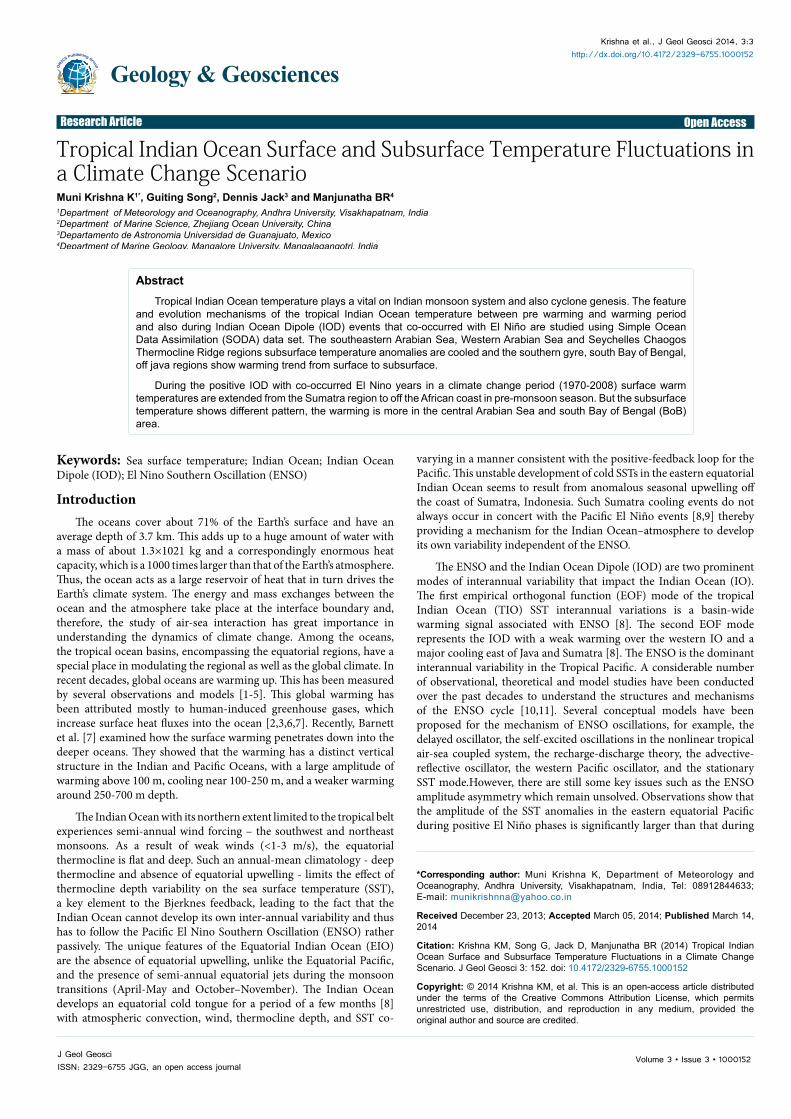
the latitude 20°N to 20°S and longitude 40°E to 120°E. Different regions are identified based on the surface and subsurface warming (cooling). Figure 1 illustrates the tropical Indian Ocean and different regions represents boxes A (Java), B (Seychelles-Chagos thermocline ridge), C (souther gyre), D (Western Arabian Sea), E (Southeast Arabian Sea), and F (south Bay of Bengal). The red color represents warming and sky blue color cooling.
Data and MethodologyThe Simple Ocean Data Assimilation (SODA) version 2.2.4 product
of Carton et al. [15] and Giese et al. [16] for 1871–2008 are used as a major dataset for the ocean diagnosis. There are several versions of SODA [17] depending on the experiment setup. Version 2.2.4 represents their first assimilation run of over 100 years and uses the 20Crv2 ensemble winds. As such, it is considered a “beta release” and is currently under evaluation and a preparation of another long run. We are releasing it as we feel it is important for other researchers to have a chance to examine it.
The ocean model is based on Parallel Ocean Program physics with an average 0.25°x0.4°x40-level resolution. Observations include virtually all available hydrographic profile data, as well as ocean station data, moored temperature and salinity time series, surface temperature
20N
15N
10N
5N
EQ
5S
10S
15S
20S40E 50E 60E 70E 80E 90E 100E 110E 120E
D
E F
A
B
C
Figure 1: Study region and the boxes represent the warming (A(Java), C( SG), F(SBoB)) and cooling (B(SCTR), D (WAS), E(SEAS)) areas.
StatisticsJF MANI JJAS OND
5m 70m 96m 5m 70m 96m 5m 70m 96m 5m 70m 96m
Min 2510, 26.02 1938, 19.57
1&03, 16.66 2718,2&32 2538, 24.62 22.84, 21.95 2536,
25.8624.66, 24.26 2234, 22.41 2439, 26.37 2114, 20.87 1909,1&99
Max 28.68, 28.59 27.86, 26.77
2537, 25.03 2935, 30.14 2837, 28.00 26.69, 27.08 28.00,
27.402735, 26.69
25.98, 25.69 2834, 28.85 2611, 25.45 24.03,
23.29Std 034, 0.56 L42,1.44 L67, /. 72 0A9,0.39 033, 0.86 0.85, 1.18 0A4,0.37 036, 0.61 a69,0.84 a65,0.40 L02,0.96 1.12, 1.06
Mean 2634, 27.10 24.95, 23.89
2237, 21.06 2&48,29.09 2&88,26.68 24.95, 24.56 2636,
26.772531, 25.64 2&63,24.10 2637, 27.50 2144, 23.49 2131, 21.46
Skewness -t103,0.25 -a66,-a49 -031,-004 -004,063 020,-063 -013,-042 038,-030 008,-060 -016,-019 012,030 015, -036 a26,-0A325th
percentile 2&60,26.72 2332, 23.00
21.18, 20.01 2813,2&84 2633, 26.68 24.26, 23.91 26.26,
26.542531, 25.24
24.10, 23.41 2633, 27.25 2232, 22.99 2031, 20.99
50th percentile 26.95, 27.03 2109,
24.092238, 20.86 28A6, 29.09 26.84,
26.91 25.07, 24.59 2635, 26.71
25.90, 25.83
24.63, 24.14 26.73, 27.50 2146, 23.64 21.16,
21.3775th
percentile 27.29, 27.50 25.99, 24.56
2333, 22.12 28.83, 29.31 27.21,
27.32 2536, 25.44 26.83, 27.08
26.27, 26.09 2109, 24.86 2714, 27.66 24.16, 24.04 21.96,
22.24Kurtosis 1.21, 0.24 1.21, 1.17 038, 0.34 -035,032 a60,-0.22 -065,-0.12 038, 0.11 -015,-039 -0A6,-032 031, 3.71 -034,134 -032,-007
Table 1: Statistics of temperature at different depths during 1871-1969 and 1970-2008 (italic) over the WAS region.
Citation: Krishna KM, Song G, Jack D, Manjunatha BR (2014) Tropical Indian Ocean Surface and Subsurface Temperature Fluctuations in a Climate Change Scenario. J Geol Geosci 3: 152. doi: 10.4172/2329-6755.1000152
Page 3 of 17
Volume 3 • Issue 3 • 1000152J Geol GeosciISSN: 2329-6755 JGG, an open access journal
and salinity, observations of various types, and nighttime infrared satellite SST data. The output is in monthly-averaged form, mapped onto a uniform 0.5°x0.5°x40- level grid. The reanalysis provides three types of variables, those well constrained by observations, those partly constrained by dynamical relationships to variables frequently observed, and those poorly constrained such as horizontal velocity divergence. It is worth noting that SODA aims for improving the upper ocean reanalysis, because data below 1000m is limited. For more information on the SODA product see Carton et al. [15,17]. In the present study temperature data (5-200m) is used to investigate the surface and subsurface warming (cooling) over the study region during the years 1871-2008.
Anomaly: Temperature difference between the period 1970-2008 and 1871-1969 period at the surface and subsurface levels.
Skewness
It is a measure of the asymmetry of a probability distribution function, and a value of 0 represents a normal distribution [18,19]. Positive skewness indicates a distribution with an asymmetric tail extending toward more positive values. Negative skewness indicates a distribution with an asymmetric tail extending toward more negative values.
Kurtosis
It characterizes the relative peakedness or flatness of a distribution compared with the normal distribution. Positive kurtosis indicates a relatively peaked distribution. Negative kurtosis indicates a relatively flat distribution.
Percentile: The k-th percentile of values in a range. This function is used to establish a threshold of acceptance. In the present study 25th, 50th and 75th percentile is calculated.
The IOD, El Niño and La Niña years are taken from Gary et al. [20]. In the 138 years after 1871, 19 negative and 17 positive dipole events have occurred according to SODA SST data (Table 1) based on the dipole mode index (DMI) calculated using the Saji et al. [8] method. In the present study the positive and negative IODs with co-occurred El Niño and La Niña years are used. The positive IOD and El Niño events during 1871-1969 are 1877, 1902, 1913, 1914, 1923, 1926, 1953, 1963 and during 1970-2008 period 1972, 1982, 1994, 1997, 2006. Negative IOD and La Niña events occurred during the 1871-1969 period in 1879, 1889, 1890, 1892, 1906, 1909, 1954, 1964 and during the 1970-2008 period in 1975, 1984, 1989.
ResultsThe monsoonal climate over the Indian subcontinent, the Equatorial
Indian Ocean and other south Asian countries is a consequence of the unique geographical settings of ocean and land masses. The SST is the key parameter for air-sea interaction processes. Thus, the study of its variability in intra and inter annual scale may provide vital information about air-sea interaction processes (heat and water fluxes) and climate in the ocean environment. We examine the intra annual variability of the sea surface temperature (SST) anomaly over the Tropical Indian Ocean based on SODA temperature data (during 1871-2008) of 0.25° x 0.4° latitude longitude grid derived from the Asia Pacific Data Research Centre. Despite a strong seasonal cycle in the IO, the annual mean picture is quite useful for understanding the dynamics and thermodynamics of various features of the thermal structure.
40E 50E 60E 70E 80E 90E 100E 110E 120E
20N
15N
10N
5N
EQ
5S
10S
15S
20S40E 50E 60E 70E 80E 90E 100E 110E 120E
20N
15N
10N
5N
EQ
5S
10S
15S
20S40E 50E 60E 70E 80E 90E 100E 110E 120E
20N
15N
10N
5N
EQ
5S
10S
15S
20S
40E 50E 60E 70E 80E 90E 100E 110E 120E
20N
15N
10N
5N
EQ
5S
10S
15S
20S
40E 50E 60E 70E 80E 90E 100E 110E 120E
20N
15N
10N
5N
EQ
5S
10S
15S
20S40E 50E 60E 70E 80E 90E 100E 110E 120E
20N
15N
10N
5N
EQ
5S
10S
15S
20S
40E 50E 60E 70E 80E 90E 100E 110E 120E
20N
15N
10N
5N
EQ
5S
10S
15S
20S40E 50E 60E 70E 80E 90E 100E 110E 120E
20N
15N
10N
5N
EQ
5S
10S
15S
20S
40E 50E 60E 70E 80E 90E 100E 110E 120E
20N
15N
10N
5N
EQ
5S
10S
15S
20S
40E 50E 60E 70E 80E 90E 100E 110E 120E
20N
15N
10N
5N
EQ
5S
10S
15S
20S40E 50E 60E 70E 80E 90E 100E 110E 120E
20N
15N
10N
5N
EQ
5S
10S
15S
20S40E 50E 60E 70E 80E 90E 100E 110E 120E
20N
15N
10N
5N
EQ
5S
10S
15S
20S
DecNovOct
Jul Aug Sep
JunMayApr
Jan Feb Mar
1.8
1.5
1.2
0.9
0.6
0.3
0
-0.3
-0.6
-0.9
-1.2
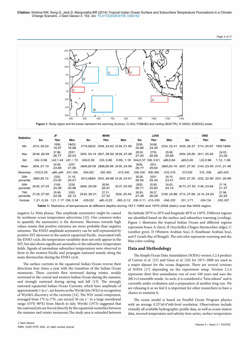
Figure 2: Monthly variation of temperature anomaly at 5m depth over the Tropical Indian Ocean.
Citation: Krishna KM, Song G, Jack D, Manjunatha BR (2014) Tropical Indian Ocean Surface and Subsurface Temperature Fluctuations in a Climate Change Scenario. J Geol Geosci 3: 152. doi: 10.4172/2329-6755.1000152
Page 4 of 17
Volume 3 • Issue 3 • 1000152J Geol GeosciISSN: 2329-6755 JGG, an open access journal
Spatio-temporal variability of SST anomaly
The distribution of the annual mean temperature at the surface, 70m and 96m depths and the corresponding standard deviation are shown in the Figures 2-4. There exists a warm temperature anomaly at the surface of the entire IO, except south of 8°S. The equatorial IO warm, unlike the pattern in other equatorial oceans where the surface is warm towards west. Regions near the Somali and the Arabian coast are cooler due to the dominance of the south-west monsoon winds that induce coastal upwelling in these regions. At 96m depths, there are pockets of warm temperature in the central Arabian Sea and Equatorial Indian Ocean (EIO). In the southern Tropical IO (TIO), at 96m depths there exists a band of warm water between 15°S to 20°S, which is intense in the east, just north of the Australian continent.
The annual evolution of the temperature anomaly at the surface (5m) and, subsurface (70m, 96m) of the Tropical Indian Ocean (TIO) are shown in Figures 2-4. Figure 2 suggest that during January there is a warm water front with a mean temperature anomaly of 1°C situated in north of the equator, which is elongated to the south east direction. During this period, south of equator exist a relatively cooler mean anomaly of -0.6°C. The Arabian Sea is relatively cooler (0.25°C) than the Bay of Bengal (0.6°C). Maximum warming (0.8°C) from the Sumatra coast to the equator up to the east coast of India is observed. A similar temperature gradient exists in the Arabian Sea with a lower SST anomaly in the western part (off the Oman coast) than the eastern part. Strong cooling is observed south of 8°S and Seychelles-Chagos thermocline ridge (SCTR), and relatively cooler water patches are seen in the ocean than its surrounding.
During February, the SST anomaly pattern is almost similar to the January SST anomaly pattern. However, the western Arabian Sea is cooler than the January pattern, and the warm SST anomaly along the east coast of India is significantly reduced. Surface cooling is further increase at the SCTR region. The equatorial warm front is relatively warmer along its eastern side (Somali coast).
During March, with the movement of the sun from the southern hemisphere to the northern hemisphere, the equatorial ocean has warmed up significantly (up to 0.9°C) and it became wider towards the Arabian Sea. Earlier cold fronts which were elongated from north Arabian Sea to central Arabian Sea. During April almost all part of the north Indian Ocean (including AS and BOB) is covered by very warm water except off the Andaman coast, and thermal equator is intensified (1.1°C) and shifted to the north. The Western Arabian Sea is up to 1.25°C warmer than the entire tropical Indian Ocean. The ocean is warmest (1.25°C) during this month. During May, the Western Arabian Sea is further warming (1.5°C) and the Bay of Bengal surface waters also show warm anomaly. However, the SCTR surface temperature anomaly is reduced compared to the April pattern.
During June, when the sun is in the extreme position in the northern hemisphere and the monsoonal wind is strong over the tropical Indian Ocean, the SST anomaly of SEAS has decreased significantly, whereas the BOB is still remaining relatively warm, in particular north of 10°N. The entire Arabian Coast is warming very rapidly during this month. The western Arabian Sea warm anomaly is slightly disturbed due to the cool water entering from the SCTR region. During this period, cold water from the Arabian Sea advects to Bay of Bengal. During July, the western Arabian Sea shows very cool waters (-0.8°C). However, the SST
40E 50E 60E 70E 80E 90E 100E 110E 120E
20N
15N
10N
5N
EQ
5S
10S
15S
20S40E 50E 60E 70E 80E 90E 100E 110E 120E
20N
15N
10N
5N
EQ
5S
10S
15S
20S
40E 50E 60E 70E 80E 90E 100E 110E 120E
20N
15N
10N
5N
EQ
5S
10S
15S
20S
40E 50E 60E 70E 80E 90E 100E 110E 120E
20N
15N
10N
5N
EQ
5S
10S
15S
20S
40E 50E 60E 70E 80E 90E 100E 110E 120E
20N
15N
10N
5N
EQ
5S
10S
15S
20S
40E 50E 60E 70E 80E 90E 100E 110E 120E
20N
15N
10N
5N
EQ
5S
10S
15S
20S
40E 50E 60E 70E 80E 90E 100E 110E 120E
20N
15N
10N
5N
EQ
5S
10S
15S
20S
40E 50E 60E 70E 80E 90E 100E 110E 120E
20N
15N
10N
5N
EQ
5S
10S
15S
20S
40E 50E 60E 70E 80E 90E 100E 110E 120E
20N
15N
10N
5N
EQ
5S
10S
15S
20S40E 50E 60E 70E 80E 90E 100E 110E 120E
20N
15N
10N
5N
EQ
5S
10S
15S
20S
40E 50E 60E 70E 80E 90E 100E 110E 120E
20N
15N
10N
5N
EQ
5S
10S
15S
20S
40E 50E 60E 70E 80E 90E 100E 110E 120E
20N
15N
10N
5N
EQ
5S
10S
15S
20S
3
2.5
2
1.5
1
0.5
0
-0.5
-1
-1.5
-2
-2.5
Jan Feb Mar
Jun
Sep
DecNovOct
Jul Aug
MayApr
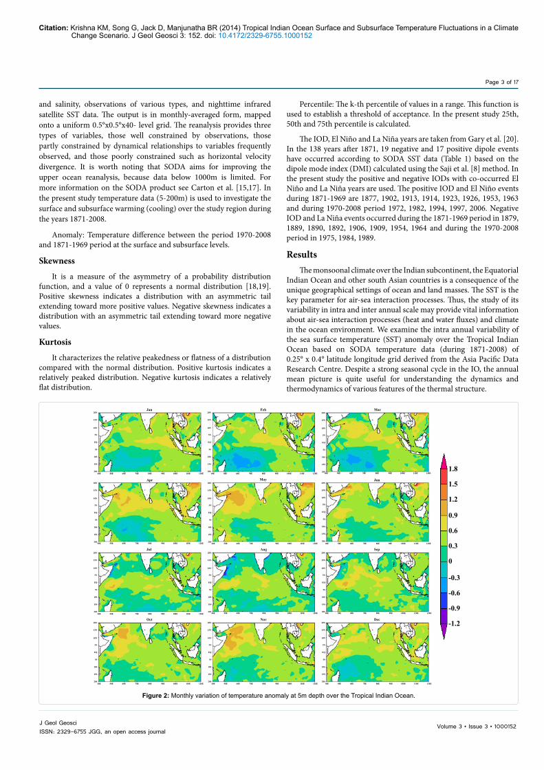
Figure 3: Monthly variation of temperature anomaly at 70m depth over the Tropical Indian Ocean.

Citation: Krishna KM, Song G, Jack D, Manjunatha BR (2014) Tropical Indian Ocean Surface and Subsurface Temperature Fluctuations in a Climate Change Scenario. J Geol Geosci 3: 152. doi: 10.4172/2329-6755.1000152
Page 5 of 17
Volume 3 • Issue 3 • 1000152J Geol GeosciISSN: 2329-6755 JGG, an open access journal
anomaly is relatively cooler in central and southeast Arabian Sea (SEAS) compared to the previous month. The cooling of the western Arabian Sea in July and August (-1.2°C) has almost a similar extent and more than the month of June. Along the east coast of India and the Arabian coast also shows significantly cooling trend during July and August. The Western Arabian Sea is relatively warmer during September than during the earlier months. The central BOB temperature anomaly increases continuously during this period. SCTR is further warming compared to the previous months.
During October and November, the warm temperature pattern of the north Indian Ocean is almost uniform over most part of the basin, but the intensity is higher at western Arabian Sea. This warming is similar to the month of May,whereas the STCR is showing a cooling trend during December, the surface warming reappears along the east coast of India. The Equatorial Indian Ocean warms up and the thermal equator reappears. This pattern is intensified during the next month of January. The Subsurface (70m and 96m) temperature anomaly shows an abrupt change compared to the surface values. Figure 3 suggest that during January, western IO from 10°S to 15°N almost cooling is observed than the eastern part at 70m depth. The cooling trend is almost -2°C and the warming trend is 2°C. The warm subsurface water flow at 70m goes from the Indonesian Throughflow (ITF) through the central EIO and the south Bay of Bengal. A weak negative temperature anomaly is observed in the SEAS than the Western Arabian Sea (WAS) region. Strong cooling is observed south of 8°S and the SCTR, relatively cooler water patches are seen in the ocean than its surrounding. During February, the SST anomaly pattern is almost similar to the January SST
anomaly pattern. However, the western Arabian Sea is less cool than the January pattern and the warm SST anomaly along the east coast of India has significantly increased. Subsurface cooling is further increasing at the SCTR region. The warming (2°C) trend has increased further off the Sumatra coast. During March, with the movement of the sun from southern hemisphere to the northern hemisphere, the Java region has warmed up significantly (up to 2°C) and it became wider towards north of the equator. The SCTR region further cooled and reached -2.5°C, but north of 7°S strong warm core eddies are observed and their movement is towards the African coast. During April, almost all part of the eastern IO (including BOB, Sumatra and Java) is covered by very warm water except for the Andaman coast. Vigorous changes are observed in the Western Arabian Sea and SEAS. The cool waters are replaced by a warm anomaly in the WAS and SEAS. Whereas north of the SCTR region the number of warm core eddies has further increased from two to three, and their movement is same as in March. The spatial extent of cool water (-2.5°C) has also increased in the SCTR region. In the month of May, two strong cooling spots are identified over thesouthern IO, one is in the SCTR region and another one is in the central EIO. The spatial extent of the two regions is almost same. Off the Java coast, the subsurface temperature anomaly has increased and reached its maximum (3.5°C). The North Indian Ocean (NIO) warm subsurface waters have occupied both sides of Indian subcontinent. The three warm core eddy shaped patterns have moved towards the African coast (5°S) and form a dumbbell shape from 5°S to equator, but one warm core region is still at 58°E, but as a weak anomaly.
During June, when the sun is in the extreme position in the northern hemisphere and monsoonal wind is strong over the tropical
40E 50E 60E 70E 80E 90E 100E 110E 120E
20N
15N
10N
5N
EQ
5S
10S
15S
20S40E 50E 60E 70E 80E 90E 100E 110E 120E
20N
15N
10N
5N
EQ
5S
10S
15S
20S
40E 50E 60E 70E 80E 90E 100E 110E 120E
20N
15N
10N
5N
EQ
5S
10S
15S
20S
40E 50E 60E 70E 80E 90E 100E 110E 120E
20N
15N
10N
5N
EQ
5S
10S
15S
20S
40E 50E 60E 70E 80E 90E 100E 110E 120E
20N
15N
10N
5N
EQ
5S
10S
15S
20S
40E 50E 60E 70E 80E 90E 100E 110E 120E
20N
15N
10N
5N
EQ
5S
10S
15S
20S
40E 50E 60E 70E 80E 90E 100E 110E 120E
20N
15N
10N
5N
EQ
5S
10S
15S
20S
40E 50E 60E 70E 80E 90E 100E 110E 120E
20N
15N
10N
5N
EQ
5S
10S
15S
20S
40E 50E 60E 70E 80E 90E 100E 110E 120E
20N
15N
10N
5N
EQ
5S
10S
15S
20S40E 50E 60E 70E 80E 90E 100E 110E 120E
20N
15N
10N
5N
EQ
5S
10S
15S
20S
40E 50E 60E 70E 80E 90E 100E 110E 120E
20N
15N
10N
5N
EQ
5S
10S
15S
20S
40E 50E 60E 70E 80E 90E 100E 110E 120E
20N
15N
10N
5N
EQ
5S
10S
15S
20S
3
2.5
2
1.5
1
0.5
-0.5
-1
-1.5
-2
-2.5
-3
Jan Feb Mar
Jun
Sep
DecNovOct
Jul Aug
MayApr
Figure 4: Monthly variation of temperature anomaly at 96m depth over the Tropical Indian Ocean.

Citation: Krishna KM, Song G, Jack D, Manjunatha BR (2014) Tropical Indian Ocean Surface and Subsurface Temperature Fluctuations in a Climate Change Scenario. J Geol Geosci 3: 152. doi: 10.4172/2329-6755.1000152
Page 6 of 17
Volume 3 • Issue 3 • 1000152J Geol GeosciISSN: 2329-6755 JGG, an open access journal
30.5
29
27.5
26
24.5
23
21.5
20
18.5
17
40E 50E 60E 70E 80E 90E 100E 110E 120E
20N
15N
10N
5N
EQ
5S
10S
15S
20S40E 50E 60E 70E 80E 90E 100E 110E 120E
20N
15N
10N
5N
EQ
5S
10S
15S
20S
40E 50E 60E 70E 80E 90E 100E 110E 120E
20N
15N
10N
5N
EQ
5S
10S
15S
20S40E 50E 60E 70E 80E 90E 100E 110E 120E
20N
15N
10N
5N
EQ
5S
10S
15S
20S
40E 50E 60E 70E 80E 90E 100E 110E 120E
20N
15N
10N
5N
EQ
5S
10S
15S
20S40E 50E 60E 70E 80E 90E 100E 110E 120E
20N
15N
10N
5N
EQ
5S
10S
15S
20S
Annual Mean Temp at 0m (deg C) Annual Mean Temp at 0m (deg C)
Annual Mean Temp at 70m (deg C)Annual Mean Temp at 70m (deg C)
Annual Mean Temp at 96m (deg C) Annual Mean Temp at 96m (deg C)
Figure 5: Annual mean and standard deviation (contours) of SODA temperature at surface (5m), 70m, 96m depth for the periods 1871-1969 (left panel), 1970-2008 (right panel).
40E 50E 60E 70E 80E 90E 100E 110E 120E
20N
15N
10N
5N
EQ
5S
10S
15S
20S
40E 50E 60E 70E 80E 90E 100E 110E 120E
20N
15N
10N
5N
EQ
5S
10S
15S
20S40E 50E 60E 70E 80E 90E 100E 110E 120E
20N
15N
10N
5N
EQ
5S
10S
15S
20S
40E 50E 60E 70E 80E 90E 100E 110E 120E
20N
15N
10N
5N
EQ
5S
10S
15S
20S
1.6
1.4
1.2
1
0.8
0.6
0.4
0.2
0
-0.2
-0.4
-0.6
MAMJF
JJAS OND
Figure 6: Mean seasonal temperature anomaly at 5m depth over the Tropical Indian Ocean.
Citation: Krishna KM, Song G, Jack D, Manjunatha BR (2014) Tropical Indian Ocean Surface and Subsurface Temperature Fluctuations in a Climate Change Scenario. J Geol Geosci 3: 152. doi: 10.4172/2329-6755.1000152
Page 7 of 17
Volume 3 • Issue 3 • 1000152J Geol GeosciISSN: 2329-6755 JGG, an open access journal
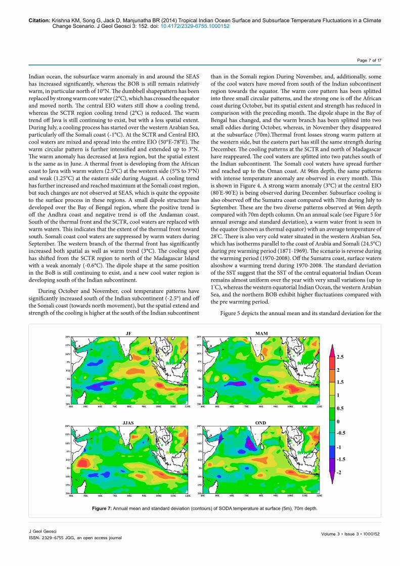
Indian ocean, the subsurface warm anomaly in and around the SEAS has increased significantly, whereas the BOB is still remain relatively warm, in particular north of 10°N. The dumbbell shapepattern has been replaced by strong warm core water (2°C), which has crossed the equator and moved north. The central EIO waters still show a cooling trend, whereas the SCTR region cooling trend (2°C) is reduced. The warm trend off Java is still continuing to exist, but with a less spatial extent. During July, a cooling process has started over the western Arabian Sea, particularly off the Somali coast (-1°C). At the SCTR and Central EIO, cool waters are mixed and spread into the entire EIO (50°E-78°E). The warm circular pattern is further intensified and extended up to 3°N. The warm anomaly has decreased at Java region, but the spatial extent is the same as in June. A thermal front is developing from the African coast to Java with warm waters (2.5°C) at the western side (5°S to 3°N) and weak (1.25°C) at the eastern side during August. A cooling trend has further increased and reached maximum at the Somali coast region, but such changes are not observed at SEAS, which is quite the opposite to the surface process in these regions. A small dipole structure has developed over the Bay of Bengal region, where the positive trend is off the Andhra coast and negative trend is off the Andaman coast. South of the thermal front and the SCTR, cool waters are replaced with warm waters. This indicates that the extent of the thermal front toward south. Somali coast cool waters are suppressed by warm waters during September. The western branch of the thermal front has significantly increased both spatial as well as warm trend (3°C). The cooling spot has shifted from the SCTR region to north of the Madagascar Island with a weak anomaly (-0.6°C). The dipole shape at the same position in the BoB is still continuing to exist, and a new cool water region is developing south of the Indian subcontinent.
During October and November, cool temperature patterns have significantly increased south of the Indian subcontinent (-2.5°) and off the Somali coast (towards north movement), but the spatial extend and strength of the cooling is higher at the south of the Indian subcontinent
than in the Somali region During November, and, additionally, some of the cool waters have moved from south of the Indian subcontinent region towards the equator. The warm core pattern has been splitted into three small circular patterns, and the strong one is off the African coast during October, but its spatial extent and strength has reduced in comparison with the preceding month. The dipole shape in the Bay of Bengal has changed, and the warm branch has been splitted into two small eddies during October, whereas, in November they disappeared at the subsurface (70m).Thermal front losses strong warm pattern at the western side, but the eastern part has still the same strength during December. The cooling patterns at the SCTR and north of Madagascar have reappeared. The cool waters are splitted into two patches south of the Indian subcontinent. The Somali cool waters have spread further and reached up to the Oman coast. At 96m depth, the same patterns with intense temperature anomaly are observed in every month. This is shown in Figure 4. A strong warm anomaly (3°C) at the central EIO (80°E-90°E) is being observed during December. Subsurface cooling is also observed off the Sumatra coast compared with 70m during July to September. These are the two diverse patterns observed at 96m depth compared with 70m depth column. On an annual scale (see Figure 5 for annual average and standard deviation), a warm water front is seen in the equator (known as thermal equator) with an average temperature of 28°C. There is also very cold water situated in the western Arabian Sea, which has isotherms parallel to the coast of Arabia and Somali (24.5°C) during pre warming period (1871-1969). The scenario is reverse during the warming period (1970-2008). Off the Sumatra coast, surface waters alsoshow a warming trend during 1970-2008. The standard deviation of the SST suggest that the SST of the central equatorial Indian Ocean remains almost uniform over the year with very small variations (up to 1°C), whereas the western equatorial Indian Ocean, the western Arabian Sea, and the northern BOB exhibit higher fluctuations compared with the pre warming period.
Figure 5 depicts the annual mean and its standard deviation for the
40E 50E 60E 70E 80E 90E 100E 110E 120E
20N
15N
10N
5N
EQ
5S
10S
15S
20S40E 50E 60E 70E 80E 90E 100E 110E 120E
20N
15N
10N
5N
EQ
5S
10S
15S
20S
40E 50E 60E 70E 80E 90E 100E 110E 120E
20N
15N
10N
5N
EQ
5S
10S
15S
20S40E 50E 60E 70E 80E 90E 100E 110E 120E
20N
15N
10N
5N
EQ
5S
10S
15S
20S
JF MAM
ONDJJAS
2.5
2
1.5
1
0.5
0
-0.5
-1
-1.5
-2
Figure 7: Annual mean and standard deviation (contours) of SODA temperature at surface (5m), 70m depth.
Citation: Krishna KM, Song G, Jack D, Manjunatha BR (2014) Tropical Indian Ocean Surface and Subsurface Temperature Fluctuations in a Climate Change Scenario. J Geol Geosci 3: 152. doi: 10.4172/2329-6755.1000152
Page 8 of 17
Volume 3 • Issue 3 • 1000152J Geol GeosciISSN: 2329-6755 JGG, an open access journal
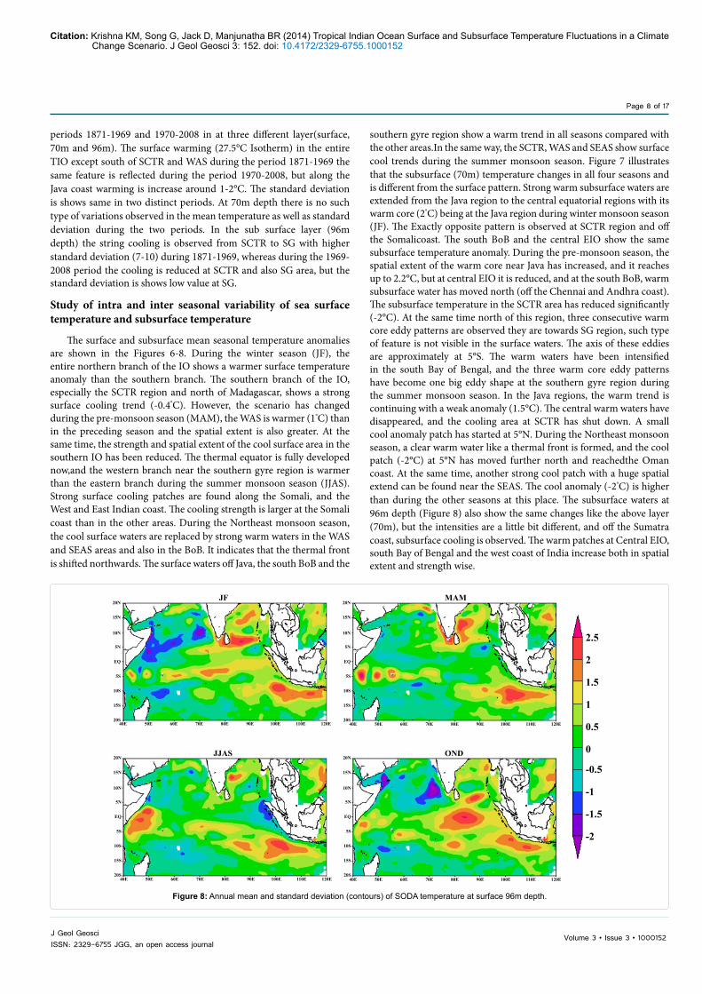
periods 1871-1969 and 1970-2008 in at three different layer(surface, 70m and 96m). The surface warming (27.5°C Isotherm) in the entire TIO except south of SCTR and WAS during the period 1871-1969 the same feature is reflected during the period 1970-2008, but along the Java coast warming is increase around 1-2°C. The standard deviation is shows same in two distinct periods. At 70m depth there is no such type of variations observed in the mean temperature as well as standard deviation during the two periods. In the sub surface layer (96m depth) the string cooling is observed from SCTR to SG with higher standard deviation (7-10) during 1871-1969, whereas during the 1969-2008 period the cooling is reduced at SCTR and also SG area, but the standard deviation is shows low value at SG.
Study of intra and inter seasonal variability of sea surface temperature and subsurface temperature
The surface and subsurface mean seasonal temperature anomalies are shown in the Figures 6-8. During the winter season (JF), the entire northern branch of the IO shows a warmer surface temperature anomaly than the southern branch. The southern branch of the IO, especially the SCTR region and north of Madagascar, shows a strong surface cooling trend (-0.4°C). However, the scenario has changed during the pre-monsoon season (MAM), the WAS is warmer (1°C) than in the preceding season and the spatial extent is also greater. At the same time, the strength and spatial extent of the cool surface area in the southern IO has been reduced. The thermal equator is fully developed now,and the western branch near the southern gyre region is warmer than the eastern branch during the summer monsoon season (JJAS). Strong surface cooling patches are found along the Somali, and the West and East Indian coast. The cooling strength is larger at the Somali coast than in the other areas. During the Northeast monsoon season, the cool surface waters are replaced by strong warm waters in the WAS and SEAS areas and also in the BoB. It indicates that the thermal front is shifted northwards. The surface waters off Java, the south BoB and the
southern gyre region show a warm trend in all seasons compared with the other areas.In the same way, the SCTR, WAS and SEAS show surface cool trends during the summer monsoon season. Figure 7 illustrates that the subsurface (70m) temperature changes in all four seasons and is different from the surface pattern. Strong warm subsurface waters are extended from the Java region to the central equatorial regions with its warm core (2°C) being at the Java region during winter monsoon season (JF). The Exactly opposite pattern is observed at SCTR region and off the Somalicoast. The south BoB and the central EIO show the same subsurface temperature anomaly. During the pre-monsoon season, the spatial extent of the warm core near Java has increased, and it reaches up to 2.2°C, but at central EIO it is reduced, and at the south BoB, warm subsurface water has moved north (off the Chennai and Andhra coast). The subsurface temperature in the SCTR area has reduced significantly (-2°C). At the same time north of this region, three consecutive warm core eddy patterns are observed they are towards SG region, such type of feature is not visible in the surface waters. The axis of these eddies are approximately at 5°S. The warm waters have been intensified in the south Bay of Bengal, and the three warm core eddy patterns have become one big eddy shape at the southern gyre region during the summer monsoon season. In the Java regions, the warm trend is continuing with a weak anomaly (1.5°C). The central warm waters have disappeared, and the cooling area at SCTR has shut down. A small cool anomaly patch has started at 5°N. During the Northeast monsoon season, a clear warm water like a thermal front is formed, and the cool patch (-2°C) at 5°N has moved further north and reachedthe Oman coast. At the same time, another strong cool patch with a huge spatial extend can be found near the SEAS. The cool anomaly (-2°C) is higher than during the other seasons at this place. The subsurface waters at 96m depth (Figure 8) also show the same changes like the above layer (70m), but the intensities are a little bit different, and off the Sumatra coast, subsurface cooling is observed. The warm patches at Central EIO, south Bay of Bengal and the west coast of India increase both in spatial extent and strength wise.
40E 50E 60E 70E 80E 90E 100E 110E 120E
20N
15N
10N
5N
EQ
5S
10S
15S
20S40E 50E 60E 70E 80E 90E 100E 110E 120E
20N
15N
10N
5N
EQ
5S
10S
15S
20S
40E 50E 60E 70E 80E 90E 100E 110E 120E
20N
15N
10N
5N
EQ
5S
10S
15S
20S40E 50E 60E 70E 80E 90E 100E 110E 120E
20N
15N
10N
5N
EQ
5S
10S
15S
20S
JJAS OND
MAMJF
2.5
2
1.5
1
0.5
0
-0.5
-1
-1.5
-2
Figure 8: Annual mean and standard deviation (contours) of SODA temperature at surface 96m depth.
Citation: Krishna KM, Song G, Jack D, Manjunatha BR (2014) Tropical Indian Ocean Surface and Subsurface Temperature Fluctuations in a Climate Change Scenario. J Geol Geosci 3: 152. doi: 10.4172/2329-6755.1000152
Page 9 of 17
Volume 3 • Issue 3 • 1000152J Geol GeosciISSN: 2329-6755 JGG, an open access journal
3
2
1
0
-1
1
0
-1
-2
2 3 4 5 6 7 8 9 10 11 12
(A) (B)
Month
Tem
pera
ture
ano
mal
y (º
C)
5m70m96m
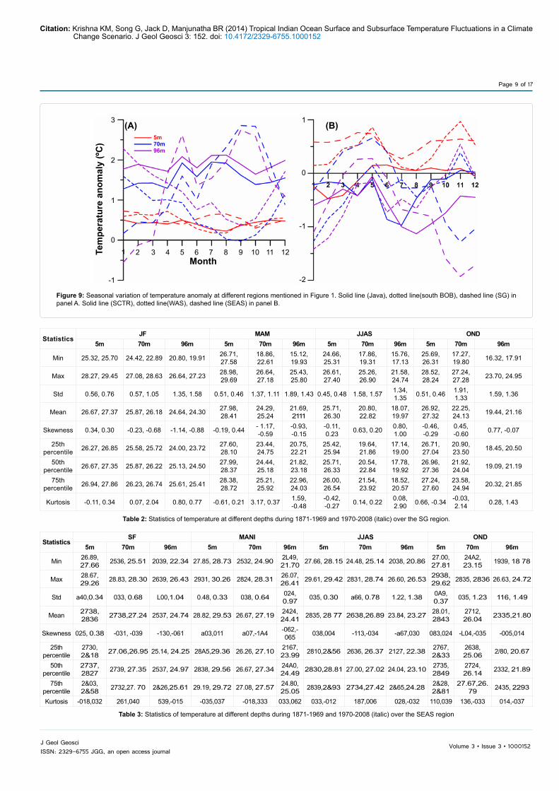
Figure 9: Seasonal variation of temperature anomaly at different regions mentioned in Figure 1. Solid line (Java), dotted line(south BOB), dashed line (SG) in panel A. Solid line (SCTR), dotted line(WAS), dashed line (SEAS) in panel B.
StatisticsJF MAM JJAS OND
5m 70m 96m 5m 70m 96m 5m 70m 96m 5m 70m 96m
Min 25.32, 25.70 24.42, 22.89 20.80, 19.91 26.71, 27.58
18.86, 22.61
15.12, 19.93
24.66, 25.31
17.86, 19.31
15.76, 17.13
25.69, 26.31
17.27, 19.80 16.32, 17.91
Max 28.27, 29.45 27.08, 28.63 26.64, 27.23 28.98, 29.69
26.64, 27.18
25.43, 25.80
26.61, 27.40
25.26, 26.90
21.58, 24.74
28.52, 28.24
27.24, 27.28 23.70, 24.95
Std 0.56, 0.76 0.57, 1.05 1.35, 1.58 0.51, 0.46 1.37, 1.11 1.89, 1.43 0.45, 0.48 1.58, 1.57 1.34, 1.35 0.51, 0.46 1.91,
1.33 1.59, 1.36
Mean 26.67, 27.37 25.87, 26.18 24.64, 24.30 27.98, 28.41
24.29, 25.24
21.69, 2111
25.71, 26.30
20.80, 22.82
18.07, 19.97
26.92, 27.32
22.25, 24.13 19.44, 21.16
Skewness 0.34, 0.30 -0.23, -0.68 -1.14, -0.88 -0.19, 0.44 - 1.17, -0.59
-0.93, -0.15
-0.11, 0.23 0.63, 0.20 0.80,
1.00-0.46, -0.29
0.45, -0.60 0.77, -0.07
25th percentile 26.27, 26.85 25.58, 25.72 24.00, 23.72 27.60,
28.1023.44, 24.75
20.75, 22.21
25.42, 25.94
19.64, 21.86
17.14, 19.00
26.71, 27.04
20.90, 23.50 18.45, 20.50
50th percentile 26.67, 27.35 25.87, 26.22 25.13, 24.50 27.99,
28.3724.44, 25.18
21.82, 23.18
25.71, 26.33
20.54, 22.84
17.78, 19.92
26.96, 27.36
21.92, 24.04 19.09, 21.19
75th percentile 26.94, 27.86 26.23, 26.74 25.61, 25.41 28.38,
28.7225.21, 25.92
22.96, 24.03
26.00, 26.54
21.54, 23.92
18.52, 20.57
27.24, 27.60
23.58, 24.94 20.32, 21.85
Kurtosis -0.11, 0.34 0.07, 2.04 0.80, 0.77 -0.61, 0.21 3.17, 0.37 1.59, -0.48
-0.42, -0.27 0.14, 0.22 0.08,
2.90 0.66, -0.34 -0.03, 2.14 0.28, 1.43
Table 2: Statistics of temperature at different depths during 1871-1969 and 1970-2008 (italic) over the SG region.
StatisticsSF MANI JJAS OND
5m 70m 96m 5m 70m 96m 5m 70m 96m 5m 70m 96m
Min 26.89, 27.66 2536, 25.51 2039, 22.34 27.85, 28.73 2532, 24.90 2L49,
21.70 27.66, 28.15 24.48, 25.14 2038, 20.86 27.00, 27.81
24A2, 23.15 1939, 18 78
Max 28.67, 29.26 28.83, 28.30 2639, 26.43 2931, 30.26 2824, 28.31 26.07,
26.41 29.61, 29.42 2831, 28.74 26.60, 26.53 2938, 29.62 2835, 2836 26.63, 24.72
Std a40,0.34 033, 0.68 L00,1.04 0.48, 0.33 038, 0.64 024, 0.97 035, 0.30 a66, 0.78 1.22, 1.38 0A9,
0.37 035, 1.23 116, 1.49
Mean 2738, 2836 2738,27.24 2537, 24.74 28.82, 29.53 26.67, 27.19 2424,
24.41 2835, 28 77 2638,26.89 23.84, 23.27 28.01, 2843
2712, 26.04 2335,21.80
Skewness 025, 0.38 -031, -039 -130,-061 a03,011 a07,-1A4 -062,-065 038,004 -113,-034 -a67,030 083,024 -L04,-035 -005,014
25th percentile
2730, 2&18 27.06,26.95 25.14, 24.25 28A5,29.36 26.26, 27.10 2167,
23.99 2810,2&56 2636, 26.37 2127, 22.38 2767, 2&33
2638, 25.06 2/80, 20.67
50th percentile
2737, 2827 2739, 27.35 2537, 24.97 2838, 29.56 26.67, 27.34 24A0,
24.49 2830,28.81 27.00, 27.02 24.04, 23.10 2735, 2849
2724, 26.14 2332, 21.89
75th percentile
2&03, 2&58 2732,27. 70 2&26,25.61 29.19, 29.72 27.08, 27.57 24.80,
25.05 2839,2&93 2734,27.42 2&65,24.28 2&28, 2&81
27.67,26. 79 2435, 2293
Kurtosis -018,032 261,040 539,-015 -035,037 -018,333 033,062 033,-012 187,006 028,-032 110,039 136,-033 014,-037
Table 3: Statistics of temperature at different depths during 1871-1969 and 1970-2008 (italic) over the SEAS region

Citation: Krishna KM, Song G, Jack D, Manjunatha BR (2014) Tropical Indian Ocean Surface and Subsurface Temperature Fluctuations in a Climate Change Scenario. J Geol Geosci 3: 152. doi: 10.4172/2329-6755.1000152
Page 10 of 17
Volume 3 • Issue 3 • 1000152J Geol GeosciISSN: 2329-6755 JGG, an open access journal
StatisticsSF MANI JJAS OND
5m 70m 96m 5m 70m 96m 5m 70m 96m 5m 70m 96m
Min 26.13, 27.20
23.06, 22.26
21.22, 19.08 26.88, 27.39 21.77, 20.72 19.27, 18.31 24.31, 24.51 23.49,
22.40 20.87, 19.66 24.39, 25.52
23.74, 23.62
22.37, 20.97
Max 30.29, 29.41
27.89, 26.76
25.34, 24.92 29.64, 29.47 26.48, 26.38 23.28, 24.22 26.70, 26.19 26.27,
25.83 24.43, 24.51 28.03, 27.61
26.67, 26.14
25.35, 25.24
Std 0.83, 0.50 0.76, 1.13 0.71, 1.50 0.58, 0.47 0.80, 1.46 0.77, 1.42 0.49, 0.49 0.57, 0.92 0.72, 1.22 0.64, 0.43 0.53, 0.58 0.53, 1.02
Mean 28.73, 28.37
24.60, 24.41
22.87, 22.34 28.32, 28.18 23.88, 23.65 21.72, 21.46 25.50, 25.59 24.87,
24.27 23.06, 22.15 26.37, 26.40
25.21, 25.20
24.30, 23.76
Skewness -0.22, -0.27 0.88, -0.18 0.26, -0.36 0.10, 0.61 0.29, -0.07 -0.25, -0.18 -0.24, -0.91 -0.22,
-0.43 -0.43, -0.03 -0.32, 0.44 -0.30, -0.88
-0.76, -0.96
25th percentile
28.09, 28.00
24.09, 23.57
22.49, 21.10 27.97, 27.89 23.45, 22.35 21.19, 20.36 25.18, 25.45 24.50,
23.89 22.59, 21.33 25.98, 26.06
24.93, 24.94
23.98, 23.33
50th percentile
28.70, 28.43
24.55, 24.54
22.90, 22.81 28.28, 28.16 23.76, 23.93 21.79, 21.77 25.56, 25.74 24.87,
24.37 23.10, 22.03 26.37, 26.43
25.22, 25.35
24.35, 23.88
75th percentile
29.44, 28.77
25.00, 25.16
23.31, 23.38 28.70, 28.44 24.37, 24.58 22.23, 22.41 25.84, 25.93 25.35,
24.87 23.61, 23.03 26.82, 26.66
25.55, 25.59
24.67, 24.38
Kurtosis -0.15, -0.22 2.77, -0.70 0.91, -0.80 -0.07, 0.64 1.16, -0.68 0.25, -0.48 -0.12, -0.21 -0.34,
-0.52 -0.05, -0.67 0.43, 0.49 0.46, 0.55 1.19, 0.67
Table 4: Statistics of temperature at different depths during 1871-1969 and 1970-2008 (italic) over the SCTR region.
StatisticsSF MANI JJAS OND
5m 70m 96m 5m 70m 96m 5m 70m 96m 5m 70m 96m
Min 27.36, 28.02 25.24, 26.89 18.33, 19.85 27.62, 28.50
23.09, 22.63
19.37, 18.80
27.40, 27.61
22.68, 23.07 19.72, 20.28 27.13, 27.48 23.60, 24.13 20.05, 20.50
Max 26.30, 27.06 22.10,2136 25.77, 26.48 29.63, 29.93
27.34, 27.52
24.03, 24.59
29.15, 28.98
27.34, 28.39 24.29, 26.10 29.04, 29.11 27.92, 28.15 25.54, 26.37
Std 28.89, 28.68 28.75, 28.47 1.34, 1.54 0.39, 0.32
0.84, 0.91
0.97, 1.10
0.34, 0.37
1.02, 1.15 0.96, 1.19 0.41, 0.36 0.88, 1.03 1.00, 1.34
Mean 0.45, 0.35 1.09, 1.15 21.85, 23.94 28.64, 29.26
24.90, 25.88
21.00, 22.42
28.02, 28.28
25.16, 25.34 21.71, 22.36 27.85, 28.32 25.30, 25.90 21.91, 23.03
Skewness 27.39, 28.00 25.26, 26.70 0.72, -0.90 0.04, -0.24
0.22, -1.08
1.25, -0.56
0.61, 0.00
0.00, 0.54 0.19, 0.64 0.67, -0.28 0.21, 0.25 0.83, 0.60
25th percentile 0.36, -0.59 0.20, -1.20 21.02, 23.31 28.37, 29.09
24.44, 25.56
20.42, 21.87
27.77, 27.94
24.41, 24.55 21.07, 21.58 27.54, 28.15 24.76, 25.03 21.18, 22.15
50th percentile 27.10, 27.83 24.57, 26.33 21.62, 24.29 28.62, 29.21
24.86, 25.82
20.87, 22.39
27.97, 28.30
25.22, 25.28 21.60, 22.24 27.82, 28.32 25.30, 25.86 21.85, 23.02
75th percentile 27.66, 28.21 25.80, 27.51 22.50, 24.90 28.91, 29.45
25.41, 26.34
21.35, 23.00
28.24, 28.57
25.71, 25.98 22.31, 22.97 28.10, 28.61 25.81, 26.66 22.48, 23.02
Kurtosis 0.70, 0.59 0.95, 1.59 0.84, 0.54 -0.24, 0.36
0.27, 3.38
1.99, 2.19
0.34, -1.03
-0.18, 0.78 -0.40, 1.22 0.29, 0.13 -0.09, -0.66 1.04, 0.21
Table 5: Statistics of temperature at different depths during 1871-1969 and 1970-2008 (italic) over the SBoB region.
The six regions (warm waters (3) and cool waters (3)) change during the seasons and are shown in Figure 9. The surface warming trend is the same in all months close to the Java region, but the warming in April, May, July and August goes to the subsurface level. The overall warm trend at subsurface level lies between 1-2°C. The south BoB shows higher warming (1.6-2.4°C) during January and February. After that it decreases until September starting to increase again and reaching 1.5°C (Figure 9a). This is very typical feature compared with the Java region. The southern gyre shows very interesting changes from the surface to the subsurface layers. At the beginning of the year (January – February), a negative anomaly (-0.5°C) has appeared, after that it starts warming up and reaches its peak value (2.6°C) during May. In the next month, the warm anomaly loses its strength again and reaches 1.2°C and reaches maximum during the second maximum (2.8°C) at the subsurface level (70m, 96m). This region is the high warming region in the IO from the surface to subsurface level, and it is very close to the equator. The statistics also show the same trend for the three warm regions (Tables 1-3).
Figure 9b shows the seasonal variation of cool waters in three regions mentioned in Figure 1(B, D, E). The surface waters at the three regions shows warm trend except SCTR region particularly during January
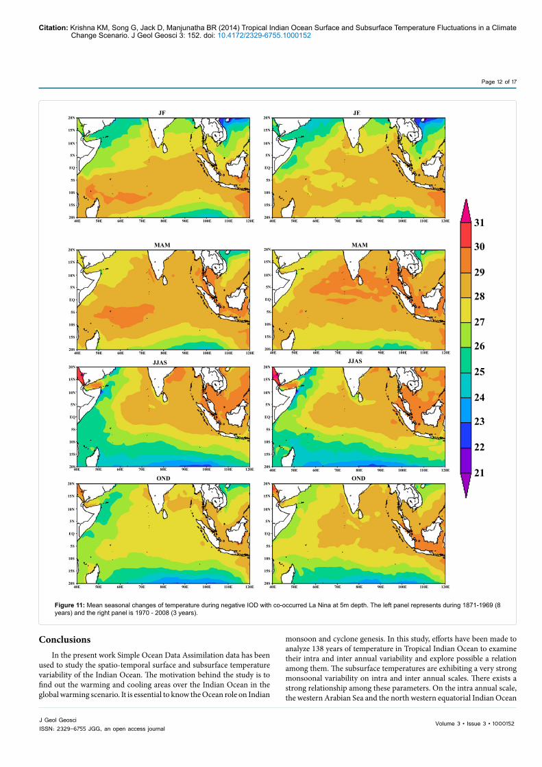
to May. The warm trend is weaker than the remaining three regions mentioned in Figure 9a. At the subsurface level, almost all months show cooling and the minimum (-1.2°C) is reached during August for the SCTR region. The SEAS and WAS regions show the same trend. During January, the anomaly is -1.4°C and it reaches maximum (-0.1°C) during pre-monsoon season and again it reaches second minimum (-2°C) at 96m depth during the month of October. The statistics also show the sametrend for these regions (Tables 4-6). During the post warming period (1970-2008) the surface waters are warmer both in spatial extent and strength wise than the pre warming period particularly in positive IOD with co-occurred El Niño years. During pre-monsoon period this situation is clearly visible (Figure 10). However, for the subsurface level a drastic change is observed during the post warming period then the pre-warming period. Surface warming regions(WAS, SCTR & SEAS) are replaced by cool water at the subsurface level (Figures 11-14). The surface warming is less during the negative IOD with co-occurred La Niña years compared with the positive IOD + El Niño years (Figure 11). The WAS region cooling trend appears in both periods (Pre and post warming periods). At the subsurface level (70m, 96m), a strong cooling patch is observed from the central EIO to the African coast and it is intensified at the SCTR region (Figures 13 and 15).

Citation: Krishna KM, Song G, Jack D, Manjunatha BR (2014) Tropical Indian Ocean Surface and Subsurface Temperature Fluctuations in a Climate Change Scenario. J Geol Geosci 3: 152. doi: 10.4172/2329-6755.1000152
Page 11 of 17
Volume 3 • Issue 3 • 1000152J Geol GeosciISSN: 2329-6755 JGG, an open access journal
40E 50E 60E 70E 80E 90E 100E 110E 120E
20N
15N
10N
5N
EQ
5S
10S
15S
20S40E 50E 60E 70E 80E 90E 100E 110E 120E
20N
15N
10N
5N
EQ
5S
10S
15S
20S
40E 50E 60E 70E 80E 90E 100E 110E 120E
20N
15N
10N
5N
EQ
5S
10S
15S
20S40E 50E 60E 70E 80E 90E 100E 110E 120E
20N
15N
10N
5N
EQ
5S
10S
15S
20S
40E 50E 60E 70E 80E 90E 100E 110E 120E
20N
15N
10N
5N
EQ
5S
10S
15S
20S
40E 50E 60E 70E 80E 90E 100E 110E 120E
20N
15N
10N
5N
EQ
5S
10S
15S
20S40E 50E 60E 70E 80E 90E 100E 110E 120E
20N
15N
10N
5N
EQ
5S
10S
15S
20S
40E 50E 60E 70E 80E 90E 100E 110E 120E
20N
15N
10N
5N
EQ
5S
10S
15S
20S
JF JF
MAMMAM
JJAS JJAS
ONDOND
31
30
29
28
27
26
25
24
23
22
21
Figure 10: Mean seasonal changes of temperature during positive IOD with co-occurred El Nino at 5m depth. The left panel represents during 1871-1969 (8 years) and the right panel is 1970 - 2008 (5 years).
StatisticsSF MANI JJAS ON'D
5m 70m 96m 5m 70m 96m 5m 70m 96m 5m 70m 96m
Min 26.89 , 27.57
21.23, 20.11
17.67, 17.07 27.22, 28.21 21.72, 22.34 18.30,
19.0925.70, 26.12
22.47, 23.40
19.30, 19.95
25.78, 26.57
21.96, 21.62 19.02, 18.51 ill
Max 29.65 , 29.57
27.77, 26.81
26.06, 24.66 29.27, 29.78 27.89, 27.72 25.04,
26.0027.84, 28.53
26.01, 27.42
23.79, 24.54
27.86, 28.32
26.49, 27.34 25.56, 24.89 17
Std 0.49, 0.43 1.25, 1.17
1.46, 1.30 0.41, 0.38 1.21, 1.19 136,
1.51 0.41, 0.47 036, 0.94
024, 1.11 -016,-0.09 0.85, /./0 1.11, 1.34
Mean 2&09,2&55 2163, 24.98
20/2, 22.06 2&41,2&86 24/6, 25.81 2038,
22.45 2635, 27.26 24.15, 25.91
2034, 22.92 2632, 27.39 24.01,
25.47 2L02,22.83 33
Skewness 015,-0.1O 036,-1.91
L05,-1.19 -014,0.58 079,-0.69 L06,0.15 -037,-016 0.40,
-0.66030,-0.70 -016,-009 035,-
1.16 L21,-0.88
25th percentile 2734,2&33 2236,
24.5319/0,
21.46 28.18, 28.61 2144, 25.27 1933, 21.67 2635, 27.01 2167,
25.3020/9,
22.23 2&62,27.14 2336, 25.07 2037, 22.10 15
50th percentile 2811,2&63 2336,
25.0720.11, 22.29 2837,2&81 24.10, 25.81 2030,
22.42 2699,27.3O 24.05, 25.98
2036, 23.24 2631, 27.41 23.99,
25.53 2034, 22.75 72
75th percentile 2845,2&76 24.17,
25.7821.08, 22.60 28.69, 29.02 24.75, 26.39 21.09,
23.33 2720, 27.52 24.61, 26.63
2135, 23.70 2726, 27.67 2430,
26.21 2149,23.77 72
Kurtosis 035, 0.15 1.12, 632
248, 5.03 -0.04, 036 0.68, 1.09 1.17, 036 0.67, L09 -034,
0.07 033,027 -037, 0.05 0.80, 3.03 237, 1.75
Table 6: Statistics of temperature at different depths during 1871-1969 and 1970-2008 (italic) over the JAVA region.
Citation: Krishna KM, Song G, Jack D, Manjunatha BR (2014) Tropical Indian Ocean Surface and Subsurface Temperature Fluctuations in a Climate Change Scenario. J Geol Geosci 3: 152. doi: 10.4172/2329-6755.1000152
Page 12 of 17
Volume 3 • Issue 3 • 1000152J Geol GeosciISSN: 2329-6755 JGG, an open access journal
40E 50E 60E 70E 80E 90E 100E 110E 120E
20N
15N
10N
5N
EQ
5S
10S
15S
20S
40E 50E 60E 70E 80E 90E 100E 110E 120E
20N
15N
10N
5N
EQ
5S
10S
15S
20S
40E 50E 60E 70E 80E 90E 100E 110E 120E
20N
15N
10N
5N
EQ
5S
10S
15S
20S40E 50E 60E 70E 80E 90E 100E 110E 120E
20N
15N
10N
5N
EQ
5S
10S
15S
20S
40E 50E 60E 70E 80E 90E 100E 110E 120E
20N
15N
10N
5N
EQ
5S
10S
15S
20S40E 50E 60E 70E 80E 90E 100E 110E 120E
20N
15N
10N
5N
EQ
5S
10S
15S
20S
40E 50E 60E 70E 80E 90E 100E 110E 120E
20N
15N
10N
5N
EQ
5S
10S
15S
20S
40E 50E 60E 70E 80E 90E 100E 110E 120E
20N
15N
10N
5N
EQ
5S
10S
15S
20S
OND OND
JJASJJAS
MAM MAM
JF JF
31
30
29
28
27
26
25
24
23
22
21
Figure 11: Mean seasonal changes of temperature during negative IOD with co-occurred La Nina at 5m depth. The left panel represents during 1871-1969 (8 years) and the right panel is 1970 - 2008 (3 years).
ConclusionsIn the present work Simple Ocean Data Assimilation data has been
used to study the spatio-temporal surface and subsurface temperature variability of the Indian Ocean. The motivation behind the study is to find out the warming and cooling areas over the Indian Ocean in the global warming scenario. It is essential to know the Ocean role on Indian
monsoon and cyclone genesis. In this study, efforts have been made to analyze 138 years of temperature in Tropical Indian Ocean to examine their intra and inter annual variability and explore possible a relation among them. The subsurface temperatures are exhibiting a very strong monsoonal variability on intra and inter annual scales. There exists a strong relationship among these parameters. On the intra annual scale, the western Arabian Sea and the north western equatorial Indian Ocean
Citation: Krishna KM, Song G, Jack D, Manjunatha BR (2014) Tropical Indian Ocean Surface and Subsurface Temperature Fluctuations in a Climate Change Scenario. J Geol Geosci 3: 152. doi: 10.4172/2329-6755.1000152
Page 13 of 17
Volume 3 • Issue 3 • 1000152J Geol GeosciISSN: 2329-6755 JGG, an open access journal
40E 50E 60E 70E 80E 90E 100E 110E 120E
20N
15N
10N
5N
EQ
5S
10S
15S
20S40E 50E 60E 70E 80E 90E 100E 110E 120E
20N
15N
10N
5N
EQ
5S
10S
15S
20S
40E 50E 60E 70E 80E 90E 100E 110E 120E
20N
15N
10N
5N
EQ
5S
10S
15S
20S40E 50E 60E 70E 80E 90E 100E 110E 120E
20N
15N
10N
5N
EQ
5S
10S
15S
20S
40E 50E 60E 70E 80E 90E 100E 110E 120E
20N
15N
10N
5N
EQ
5S
10S
15S
20S40E 50E 60E 70E 80E 90E 100E 110E 120E
20N
15N
10N
5N
EQ
5S
10S
15S
20S
40E 50E 60E 70E 80E 90E 100E 110E 120E
20N
15N
10N
5N
EQ
5S
10S
15S
20S40E 50E 60E 70E 80E 90E 100E 110E 120E
20N
15N
10N
5N
EQ
5S
10S
15S
20S
OND OND
JJAS JJAS
MAMMAM
JF JF
28
27
26
25
24
23
22
21
20
19
18
17
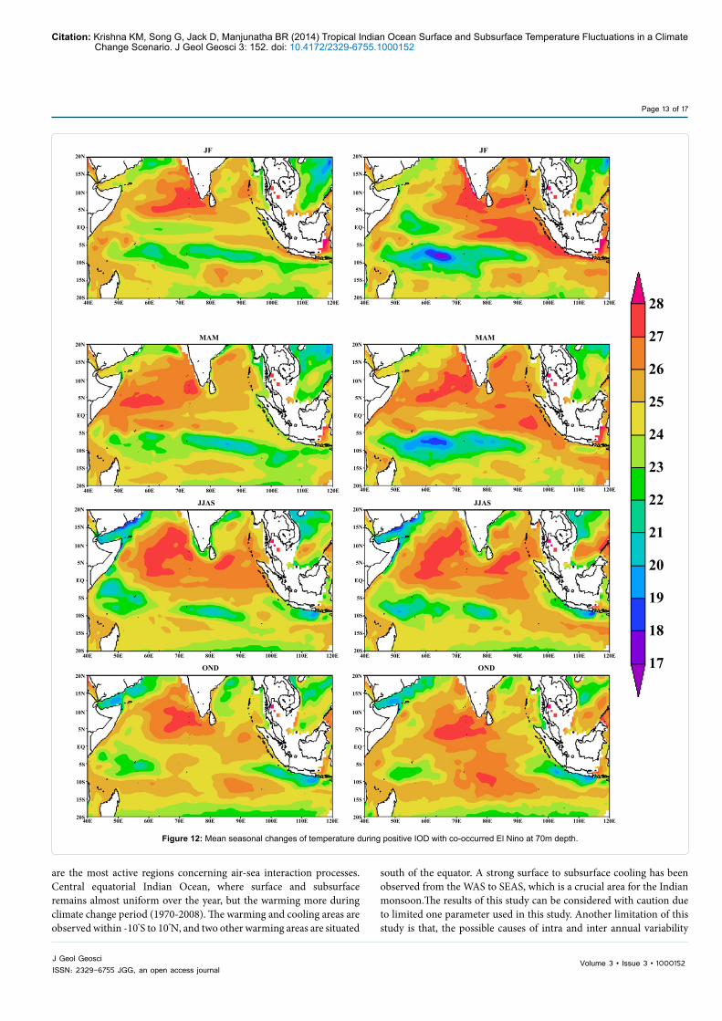
Figure 12: Mean seasonal changes of temperature during positive IOD with co-occurred El Nino at 70m depth.
are the most active regions concerning air-sea interaction processes. Central equatorial Indian Ocean, where surface and subsurface remains almost uniform over the year, but the warming more during climate change period (1970-2008). The warming and cooling areas are observed within -10°S to 10°N, and two other warming areas are situated
south of the equator. A strong surface to subsurface cooling has been observed from the WAS to SEAS, which is a crucial area for the Indian monsoon.The results of this study can be considered with caution due to limited one parameter used in this study. Another limitation of this study is that, the possible causes of intra and inter annual variability

Citation: Krishna KM, Song G, Jack D, Manjunatha BR (2014) Tropical Indian Ocean Surface and Subsurface Temperature Fluctuations in a Climate Change Scenario. J Geol Geosci 3: 152. doi: 10.4172/2329-6755.1000152
Page 14 of 17
Volume 3 • Issue 3 • 1000152J Geol GeosciISSN: 2329-6755 JGG, an open access journal
40E 50E 60E 70E 80E 90E 100E 110E 120E
20N
15N
10N
5N
EQ
5S
10S
15S
20S40E 50E 60E 70E 80E 90E 100E 110E 120E
20N
15N
10N
5N
EQ
5S
10S
15S
20S
40E 50E 60E 70E 80E 90E 100E 110E 120E
20N
15N
10N
5N
EQ
5S
10S
15S
20S40E 50E 60E 70E 80E 90E 100E 110E 120E
20N
15N
10N
5N
EQ
5S
10S
15S
20S
40E 50E 60E 70E 80E 90E 100E 110E 120E
20N
15N
10N
5N
EQ
5S
10S
15S
20S 40E 50E 60E 70E 80E 90E 100E 110E 120E
20N
15N
10N
5N
EQ
5S
10S
15S
20S
40E 50E 60E 70E 80E 90E 100E 110E 120E
20N
15N
10N
5N
EQ
5S
10S
15S
20S40E 50E 60E 70E 80E 90E 100E 110E 120E
20N
15N
10N
5N
EQ
5S
10S
15S
20S
ONDOND
JJAS JJAS
MAM MAM
JF JF
28
27
26
25
24
23
22
21
20
19
18
17
Figure 13: Mean seasonal changes of temperature during negative IOD with co-occurred La Nina at 70m depth.
exhibited in temperature is explored though qualitative arguments and no attempt is made to find the explanation. In future investigation, attempts need to be made to improve our qualitative interpretation with more dynamical data sets along with in situ observations.
Acknowledgments
We thank the SODA Project team for the production and distribution of the data used in this manuscript. We would like to acknowledge the
Citation: Krishna KM, Song G, Jack D, Manjunatha BR (2014) Tropical Indian Ocean Surface and Subsurface Temperature Fluctuations in a Climate Change Scenario. J Geol Geosci 3: 152. doi: 10.4172/2329-6755.1000152
Page 15 of 17
Volume 3 • Issue 3 • 1000152J Geol GeosciISSN: 2329-6755 JGG, an open access journal
40E 50E 60E 70E 80E 90E 100E 110E 120E
20N
15N
10N
5N
EQ
5S
10S
15S
20S
40E 50E 60E 70E 80E 90E 100E 110E 120E
20N
15N
10N
5N
EQ
5S
10S
15S
20S
40E 50E 60E 70E 80E 90E 100E 110E 120E
20N
15N
10N
5N
EQ
5S
10S
15S
20S
40E 50E 60E 70E 80E 90E 100E 110E 120E
20N
15N
10N
5N
EQ
5S
10S
15S
20S40E 50E 60E 70E 80E 90E 100E 110E 120E
20N
15N
10N
5N
EQ
5S
10S
15S
20S
40E 50E 60E 70E 80E 90E 100E 110E 120E
20N
15N
10N
5N
EQ
5S
10S
15S
20S
40E 50E 60E 70E 80E 90E 100E 110E 120E
20N
15N
10N
5N
EQ
5S
10S
15S
20S
40E 50E 60E 70E 80E 90E 100E 110E 120E
20N
15N
10N
5N
EQ
5S
10S
15S
20S
26
25
24
23
22
21
20
19
18
17
16
15
JF JF
MAMMAM
JJAS JJAS
OND OND
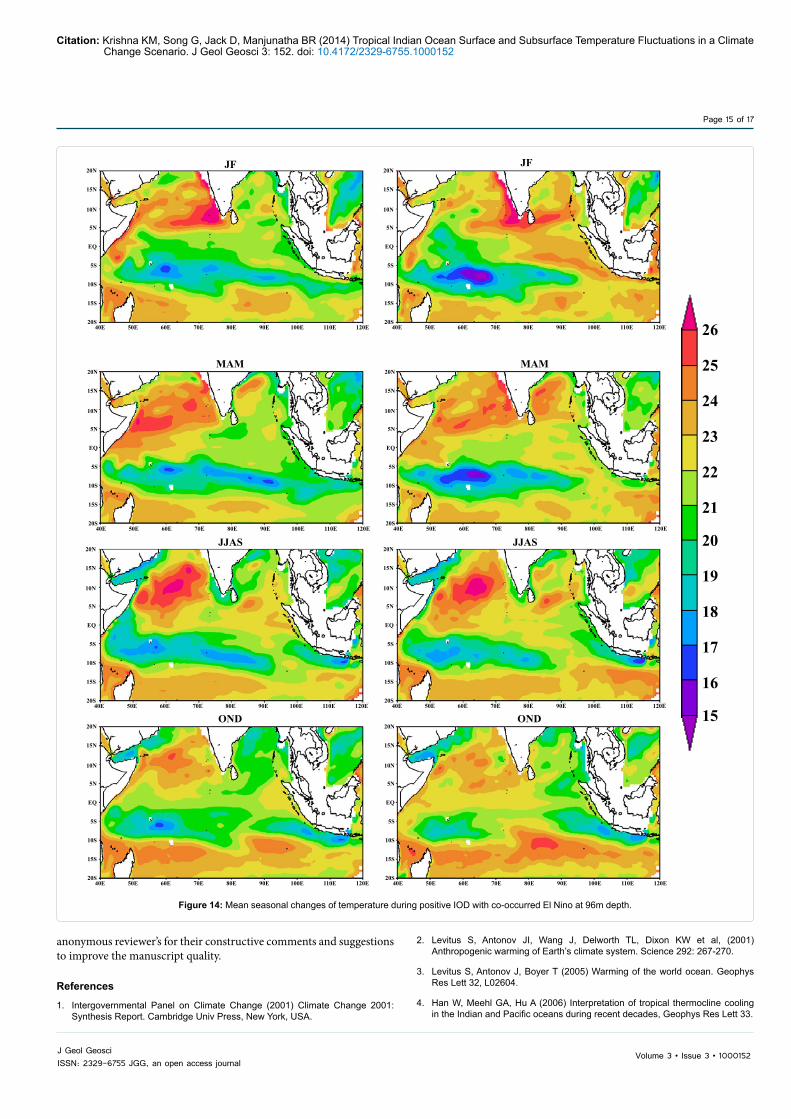
Figure 14: Mean seasonal changes of temperature during positive IOD with co-occurred El Nino at 96m depth.
anonymous reviewer’s for their constructive comments and suggestions to improve the manuscript quality.
References
1. Intergovernmental Panel on Climate Change (2001) Climate Change 2001: Synthesis Report. Cambridge Univ Press, New York, USA.
2. Levitus S, Antonov JI, Wang J, Delworth TL, Dixon KW et al, (2001) Anthropogenic warming of Earth’s climate system. Science 292: 267-270.
3. Levitus S, Antonov J, Boyer T (2005) Warming of the world ocean. Geophys Res Lett 32, L02604.
4. Han W, Meehl GA, Hu A (2006) Interpretation of tropical thermocline cooling in the Indian and Pacific oceans during recent decades, Geophys Res Lett 33.
Citation: Krishna KM, Song G, Jack D, Manjunatha BR (2014) Tropical Indian Ocean Surface and Subsurface Temperature Fluctuations in a Climate Change Scenario. J Geol Geosci 3: 152. doi: 10.4172/2329-6755.1000152
Page 16 of 17
Volume 3 • Issue 3 • 1000152J Geol GeosciISSN: 2329-6755 JGG, an open access journal
40E 50E 60E 70E 80E 90E 100E 110E 120E
20N
15N
10N
5N
EQ
5S
10S
15S
20S40E 50E 60E 70E 80E 90E 100E 110E 120E
20N
15N
10N
5N
EQ
5S
10S
15S
20S
40E 50E 60E 70E 80E 90E 100E 110E 120E
20N
15N
10N
5N
EQ
5S
10S
15S
20S40E 50E 60E 70E 80E 90E 100E 110E 120E
20N
15N
10N
5N
EQ
5S
10S
15S
20S
40E 50E 60E 70E 80E 90E 100E 110E 120E
20N
15N
10N
5N
EQ
5S
10S
15S
20S40E 50E 60E 70E 80E 90E 100E 110E 120E
20N
15N
10N
5N
EQ
5S
10S
15S
20S
40E 50E 60E 70E 80E 90E 100E 110E 120E
20N
15N
10N
5N
EQ
5S
10S
15S
20S40E 50E 60E 70E 80E 90E 100E 110E 120E
20N
15N
10N
5N
EQ
5S
10S
15S
20S
OND OND
JJAS JJAS
MAM MAM
JF JF
26
25
24
23
22
21
20
19
18
17
16
15
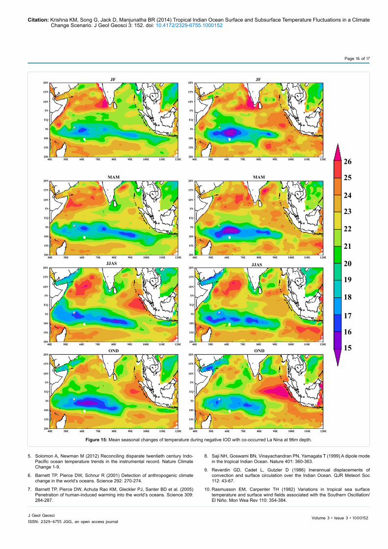
Figure 15: Mean seasonal changes of temperature during negative IOD with co-occurred La Nina at 96m depth.
5. Solomon A, Newman M (2012) Reconciling disparate twentieth century Indo-Pacific ocean temperature trends in the instrumental record. Nature Climate Change 1-9.
6. Barnett TP, Pierce DW, Schnur R (2001) Detection of anthropogenic climate change in the world’s oceans. Science 292: 270-274.
7. Barnett TP, Pierce DW, Achuta Rao KM, Gleckler PJ, Santer BD et al. (2005) Penetration of human-induced warming into the world’s oceans. Science 309: 284-287.
8. Saji NH, Goswami BN, Vinayachandran PN, Yamagata T (1999) A dipole mode in the tropical Indian Ocean. Nature 401: 360-363.
9. Reverdin GD, Cadet L, Gutzler D (1986) Inerannual displacements of convection and surface circulation over the Indian Ocean. QJR Meteorl Soc 112: 43-67.
10. Rasmusson EM, Carpenter TH (1982) Variations in tropical sea surface temperature and surface wind fields associated with the Southern Oscillation/El Niño. Mon Wea Rev 110: 354-384.
Citation: Krishna KM, Song G, Jack D, Manjunatha BR (2014) Tropical Indian Ocean Surface and Subsurface Temperature Fluctuations in a Climate Change Scenario. J Geol Geosci 3: 152. doi: 10.4172/2329-6755.1000152
Page 17 of 17
Volume 3 • Issue 3 • 1000152J Geol GeosciISSN: 2329-6755 JGG, an open access journal
11. Philander SGH (1990) El Niño, La Niña, and the Southern Oscillation, Academic Press.
12. Su JZ, Zhang R, Li T, Rong X, Kug JS, et al, (2009) Causes of the El Niño and La Niña amplitude asymmetry in the equatorial eastern Pacific. J Climate (In press) 23: 605-617.
13. Schott FA, Dengler M, Schoenefeldt R (2002) The shallow overturning circulation of the Indian Ocean. Prog Oceanogr 53: 57-103.
14. Wyrtki K (1973) An equatorial jet in the Indian Ocean. Science 181: 262-264.
15. Carton JA, Giese BS (2008) A Reanalysis of Ocean Climate Using Simple Ocean Data Assimilation (SODA). Mon Wea Rev 136: 2999-3017.
16. Giese BS, Ray S (2011) El Niño variability in simple ocean data assimilation (SODA), 1871-2008. J Geophys Res 116.
17. Carton JA, Giese BS, Grodsky SA (2005) Sea level rise and the warming of the oceans in the Simple Ocean Data Assimilation (SODA) ocean reanalysis. J Geophys Res 110.
18. Zar JH (1999) Biostatistical Analysis, 4th edition. Prentice Hall.
19. White HG (1980) Skewness, kurtosis and extreme values of Northern Hemisphere geopotential heights. Mon Wea Rev 108: 1446-1445.
20. Gary G, Subrahmanyam B, Murty VSN, Giese BS (2013) Sea Surface Salinity Variability during the Indian Ocean Dipole and ENSO Events in the Tropical Indian Ocean. J Geophys Res (C: Oceans) 116.
Citation: Krishna KM, Song G, Jack D, Manjunatha BR (2014) Tropical Indian Ocean Surface and Subsurface Temperature Fluctuations in a Climate Change Scenario. J Geol Geosci 3: 152. doi: 10.4172/2329-6755.1000152
Submit your next manuscript and get advantages of OMICS Group submissionsUnique features:
User friendly/feasible website-translation of your paper to 50 world’s leading languagesAudio Version of published paperDigital articles to share and explore
Special features:
350 Open Access Journals30,000 editorial team21 days rapid review processQuality and quick editorial, review and publication processingIndexing at PubMed (partial), Scopus, EBSCO, Index Copernicus and Google Scholar etcSharing Option: Social Networking EnabledAuthors, Reviewers and Editors rewarded with online Scientific CreditsBetter discount for your subsequent articles
Submit your manuscript at: http://www.omicsonline.org/submission