Risk Aggregation with Dependence Uncertainty - … · Model uncertainty on the risk assessment of an ... Risk and Insurance ... R. Wang, (2013) Risk Aggregation with Dependence Uncertainty,

Risk Aggregationwith Dependence Uncertainty

Carole Bernard

(Grenoble Ecole de Management)

Hannover,Current challenges in Actuarial Mathematics

November 2015

Carole Bernard Risk Aggregation with Dependence Uncertainty 1

Model Risk Unconstrained VaR bounds Dependence Information Examples 1 and 2 Example 3 Conclusions

Motivation on VaR aggregation with dependence uncertainty

Full information on marginal distributions:Xj ∼ Fj

+

Full Information on dependence:(known copula)

⇒

VaRq (X1 + X2 + ...+ Xn) can be computed!



Motivation on VaR aggregation with dependence uncertainty

Full information on marginal distributions:Xj ∼ Fj

+

Partial or no Information on dependence:(incomplete information on copula)

⇒

VaRq (X1 + X2 + ...+ Xn) cannot be computed!

Only a range of possible values for VaRq (X1 + X2 + ...+ Xn).



Model Risk

1 Goal: Assess the risk of a portfolio sum S =∑d

i=1 Xi .

2 Choose a risk measure ρ(·): variance, Value-at-Risk...

3 “Fit” a multivariate distribution for (X1,X2, ...,Xd) andcompute ρ(S)

4 How about model risk? How wrong can we be?

Assume ρ(S) = var(S),

ρ+F := sup

{var

(d∑

i=1

Xi

)}, ρ−F := inf

{var

(d∑

i=1

Xi

)}

where the bounds are taken over all other (joint distributions of)random vectors (X1,X2, ...,Xd) that “agree” with the availableinformation F



Model Risk

1 Goal: Assess the risk of a portfolio sum S =∑d

i=1 Xi .

2 Choose a risk measure ρ(·): variance, Value-at-Risk...

3 “Fit” a multivariate distribution for (X1,X2, ...,Xd) andcompute ρ(S)

4 How about model risk? How wrong can we be?

Assume ρ(S) = var(S),

ρ+F := sup

{var

(d∑

i=1

Xi

)}, ρ−F := inf

{var

(d∑

i=1

Xi

)}

where the bounds are taken over all other (joint distributions of)random vectors (X1,X2, ...,Xd) that “agree” with the availableinformation F



Aggregation with dependence uncertainty:Example - Credit Risk

I Marginals known:

I Dependence fully unknown

Consider a portfolio of 10,000 loans all having a default probabilityp = 0.049. The default correlation is ρ = 0.0157 (for KMV).

KMV VaRq Max VaRq Min VaRq

q = 0.95 10.1% 98% 0%q = 0.995 15.1% 100% 4.4%

Portfolio models are subject to significant model uncertainty(defaults are rare and correlated events).Using dependence information is crucial to try to get more“reasonable” bounds.



Objectives and Findings

� Model uncertainty on the risk assessment of an aggregateportfolio: the sum of d dependent risks.

I Given all information available in the market, what can we sayabout the maximum and minimum possible values of a givenrisk measure of a portfolio?

� Implications:

I Current VaR based regulation is subject to high model risk,even if one knows the multivariate distribution “almostcompletely”.



Objectives and Findings

� Model uncertainty on the risk assessment of an aggregateportfolio: the sum of d dependent risks.

I Given all information available in the market, what can we sayabout the maximum and minimum possible values of a givenrisk measure of a portfolio?

� Implications:

I Current VaR based regulation is subject to high model risk,even if one knows the multivariate distribution “almostcompletely”.



Acknowledgement of Collaboration

with M. Denuit, X. Jiang, L. Ruschendorf, S. Vanduffel, J. Yao, R.Wang including

• Bernard, C., Ruschendorf, L., Vanduffel, S. (2015).Value-at-Risk bounds with variance constraints. Journal ofRisk and Insurance

• Bernard, C., Vanduffel, S. (2015). A new approach toassessing model risk in high dimensions. Journal of Bankingand Finance

• Bernard, C. , Ruschendorf, L., Vanduffel, S., Yao, J. (2015).How robust is the Value-at-Risk of credit risk portfolios?European Journal of Finance

• Bernard, C., X. Jiang, R. Wang, (2013) Risk Aggregation withDependence Uncertainty, Insurance: Mathematics andEconomics



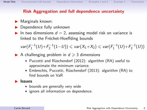
Risk Aggregation and full dependence uncertainty

I Marginals known:


I In two dimensions d = 2, assessing model risk on variance islinked to the Frechet-Hoeffding bounds

var(F−11 (U)+F−12 (1−U)) 6 var(X1+X2) 6 var(F−11 (U)+F−12 (U))

I A challenging problem in d > 3 dimensions

� Puccetti and Ruschendorf (2012): algorithm (RA) useful toapproximate the minimum variance.

� Embrechts, Puccetti, Ruschendorf (2013): algorithm (RA) tofind bounds on VaR

I Issues� bounds are generally very wide� ignore all information on dependence.

I Our answer:� incorporating in a natural way dependence information.



Risk Aggregation and full dependence uncertainty

I Marginals known:


I In two dimensions d = 2, assessing model risk on variance islinked to the Frechet-Hoeffding bounds

var(F−11 (U)+F−12 (1−U)) 6 var(X1+X2) 6 var(F−11 (U)+F−12 (U))

I A challenging problem in d > 3 dimensions



I Issues� bounds are generally very wide� ignore all information on dependence.

I Our answer:� incorporating in a natural way dependence information.



VaR Bounds with full dependence uncertainty

(Unconstrained VaR bounds)



“Riskiest” Dependence: maximum VaRq in 2 dims

If X1 and X2 are U(0,1) comonotonic, then

VaRq(Sc) = VaRq(X1) + VaRq(X2) = 2q.

q

q




If X1 and X2 are U(0,1) comonotonic, then

VaRq(Sc) = VaRq(X1) + VaRq(X2) = 2q.

q

q

Note that TVaRq)(Sc) =∫ 1q 2pdp/(1− q) = 1 + q.




If X1 and X2 are U(0,1) and antimonotonic in the tail, thenVaRq(S∗) = 1 + q.

q

q

VaRq(S∗) = 1 + q > VaRq(Sc) = 2q

⇒ to maximize VaRq, the idea is to change the comonotonicdependence such that the sum is constant in the tail



VaR at level q of the comonotonic sum w.r.t. q

p 1 q

VaRq(Sc)



VaR at level q of the comonotonic sum w.r.t. q

p 1 q

VaRq(Sc)

TVaRq(Sc)

where TVaR (Expected shortfall):TVaRq(X ) =1

1− q

∫ 1

qVaRu(X )du q ∈ (0, 1)



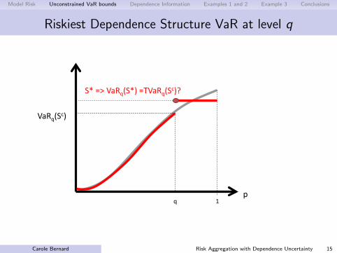
Riskiest Dependence Structure VaR at level q

p 1 q

VaRq(Sc)

S* => VaRq(S*) =TVaRq(Sc)?



Analytic expressions (not sharp)

Analytical Unconstrained Bounds with Xj ∼ Fj

A = LTVaRq(Sc) 6 VaRq [X1 + X2 + ...+ Xn] 6 B = TVaRq(Sc)

p 1 q

B:=TVaRq(Sc)

A:=LTVaRq(Sc)



VaR Bounds with full dependence uncertainty

Approximate sharp bounds:





Illustration for the maximum VaR (1/3)

8 0 3 10 1 4 11 7 7 12 8 9

1-q

q

Sum= 11

Sum= 15

Sum= 25

Sum= 29




8 0 3 10 1 4 11 7 7 12 8 9

1-q

q

Sum= 11

Sum= 15

Sum= 25

Sum= 29

Rearrange within columns..to make the sums as constant as possible… B=(11+15+25+29)/4=20




8 8 4 10 7 3 12 1 7 11 0 9

1-q

q

Sum= 20

Sum= 20

Sum= 20

Sum= 20

=B!



VaR Bounds with partial dependence uncertainty

VaR Bounds with Dependence Information...



Adding dependence information

Finding minimum and maximum possible values for VaR of thecredit portfolio loss, S =

∑ni=1 Xi , given that

� known marginal distributions of the risks Xi .

� some dependence information.

Example 1: variance constraint - with Ruschendorf and Vanduffel

M := supVaRq [X1 + X2 + ...+ Xn] ,subject to Xj ∼ Fj , var(X1 + X2 + ...+ Xn) 6 s2

Example 2: Moments constraint - with Denuit, Ruschendorf,Vanduffel, Yao

M := supVaRq [X1 + X2 + ...+ Xn] ,subject to Xj ∼ Fj ,E(X1 + X2 + ...+ Xn)k 6 ck



Adding dependence information

Example 3: VaR bounds when the joint distribution of(X1,X2, ...,Xn) is known on a subset of the sample space: withVanduffel.

Example 4: with Ruschendorf, Vanduffel and Wang

M := supVaRq [X1 + X2 + ...+ Xn] ,subject to (Xj ,Z ) ∼ Hj ,

where Z is a factor.



Examples 1 and 2

Example 1: variance constraint

M := supVaRq [X1 + X2 + ...+ Xn] ,subject to Xj ∼ Fj , var(X1 + X2 + ...+ Xn) 6 s2

Example 2: Moments constraint

M := supVaRq [X1 + X2 + ...+ Xn] ,subject to Xj ∼ Fj ,E(X1 + X2 + ...+ Xn)k 6 ck

for all k in 2,...,K



VaR bounds with moment constraints

I Without moment constraints, VaR bounds are attained ifthere exists a dependence among risks Xi such that

S =

{A probability qB probability 1− q

a.s.

� If the “distance” between A and B is too wide then improvedbounds are obtained with

S∗=

{a with probability qb with probability 1− q

such that {akq + bk(1− q) 6 ckaq + b(1− q) = E [S ]

in which a and b are “as distant as possible while satisfying allconstraints”(for all k)



Corporate portfolio

I a corporate portfolio of a major European Bank.

I 4495 loans mainly to medium sized and large corporate clients

I total exposure (EAD) is 18642.7 (million Euros), and the top10% of the portfolio (in terms of EAD) accounts for 70.1% ofit.

I portfolio exhibits some heterogeneity.

Summary statistics of a corporate portfolio

Minimum Maximum Average

Default probability 0.0001 0.15 0.0119EAD 0 750.2 116.7LGD 0 0.90 0.41



Comparison of Industry Models

VaRs of a corporate portfolio under different industry models

q = Comon. KMV Credit Risk+ Beta

95% 393.5 281.3 281.8 282.595% 393.5 340.6 346.2 347.4

ρ = 0.10 99% 2374.1 539.4 513.4 520.299.5% 5088.5 631.5 582.9 593.5



VaR bounds

With ρ = 0.1,

VaR assessment of a corporate portfolioq = KMV Comon. Unconstrained K = 2 K = 395% 340.6 393.3 (34.0 ; 2083.3) (97.3 ; 614.8) (100.9 ; 562.8)99% 539.4 2374.1 (56.5 ; 6973.1) (111.8 ; 1245) (115.0 ; 941.2)

99.5% 631.5 5088.5 (89.4 ; 10120) (114.9 ; 1709) (117.6 ; 1177.8)

� Obs 1: Comparison with analytical bounds

� Obs 2: Significant bounds reduction with momentsinformation

� Obs 3: Significant model risk



Example 3

Example 3: VaR bounds when the joint distribution of(X1,X2, ...,Xn) is known on a subset of the sample space.



Bounds on variance

Analytical Bounds on Standard Deviation

Consider d risks Xi with standard deviation σi

0 6 std(X1 + X2 + ...+ Xd) 6 σ1 + σ2 + ...+ σd

Example with 20 standard normal N(0,1)

0 6 std(X1 + X2 + ...+ X20) 6 20

and in this case, both bounds are sharp but too wide for practicaluse!Our idea: Incorporate information on dependence.



Bounds on variance

Analytical Bounds on Standard Deviation

Consider d risks Xi with standard deviation σi

0 6 std(X1 + X2 + ...+ Xd) 6 σ1 + σ2 + ...+ σd

Example with 20 standard normal N(0,1)

0 6 std(X1 + X2 + ...+ X20) 6 20

and in this case, both bounds are sharp but too wide for practicaluse!Our idea: Incorporate information on dependence.



Illustration with 2 risks with marginals N(0,1)

−3 −2 −1 0 1 2 3

−3

−2

−1

0

1

2

3

X1

X2



Illustration with 2 risks with marginals N(0,1)

−3 −2 −1 0 1 2 3

−3

−2

−1

0

1

2

3

X1

X2

Assumption: Independence on F =2⋂

k=1

{qβ 6 Xk 6 q1−β}



Illustration with marginals N(0,1)

−3 −2 −1 0 1 2 3

−3

−2

−1

0

1

2

3

X1

X2

−3 −2 −1 0 1 2 3

−3

−2

−1

0

1

2

3

X1

X2




−3 −2 −1 0 1 2 3

−3

−2

−1

0

1

2

3

X1

X2

F1 =2⋂

k=1

{qβ 6 Xk 6 q1−β}




F1 =2⋂

k=1

{qβ 6 Xk 6 q1−β} F =2⋃

k=1

{Xk > qp}⋃F1




F1 =contour of MVN at β F =2⋃

k=1

{Xk > qp}⋃F1



Our assumptions on the cdf of (X1,X2, ...,Xd)

F ⊂ Rd (“trusted” or “fixed” area)U =Rd\F (“untrusted”).We assume that we know:

(i) the marginal distribution Fi of Xi on R for i = 1, 2, ..., d ,

(ii) the distribution of (X1,X2, ...,Xd) | {(X1,X2, ...,Xd) ∈ F}.(iii) P ((X1,X2, ...,Xd) ∈ F)

I When only marginals are known: U = Rd and F = ∅.I Our Goal: Find bounds on var(S) := var(X1 + ...+ Xd)

when (X1, ...,Xd) satisfy (i), (ii) and (iii).



Our assumptions on the cdf of (X1,X2, ...,Xd)

F ⊂ Rd (“trusted” or “fixed” area)U =Rd\F (“untrusted”).We assume that we know:

(i) the marginal distribution Fi of Xi on R for i = 1, 2, ..., d ,

(ii) the distribution of (X1,X2, ...,Xd) | {(X1,X2, ...,Xd) ∈ F}.(iii) P ((X1,X2, ...,Xd) ∈ F)

I When only marginals are known: U = Rd and F = ∅.I Our Goal: Find bounds on var(S) := var(X1 + ...+ Xd)

when (X1, ...,Xd) satisfy (i), (ii) and (iii).



Example d = 20 risks N(0,1)

I (X1, ...,X20) correlated N(0,1) on

F := [qβ, q1−β]d ⊂ Rd pf = P ((X1, ...,X20) ∈ F)

(for some β 6 50%) where qγ : γ-quantile of N(0,1)

I β = 0%: no uncertainty (20 correlated N(0,1))

I β = 50%: full uncertainty

U = ∅ pf ≈ 98% pf ≈ 82% U = Rd

F = [qβ , q1−β]d β = 0% β = 0.05% β = 0.5% β = 50%ρ = 0 4.47 (4.4 , 5.65) (3.89 , 10.6) (0 , 20)

Model risk on the volatility of a portfolio is reduced a lot byincorporating information on dependence!



Example d = 20 risks N(0,1)

I (X1, ...,X20) correlated N(0,1) on

F := [qβ, q1−β]d ⊂ Rd pf = P ((X1, ...,X20) ∈ F)

(for some β 6 50%) where qγ : γ-quantile of N(0,1)

I β = 0%: no uncertainty (20 correlated N(0,1))

I β = 50%: full uncertainty

U = ∅ pf ≈ 98% pf ≈ 82% U = Rd

F = [qβ , q1−β]d β = 0% β = 0.05% β = 0.5% β = 50%ρ = 0 4.47 (4.4 , 5.65) (3.89 , 10.6) (0 , 20)

Model risk on the volatility of a portfolio is reduced a lot byincorporating information on dependence!



Numerical Results for VaR, 20 risks N(0, 1)

When marginal distributions are given,

� What is the maximum Value-at-Risk?

� What is the minimum Value-at-Risk?

� A portfolio of 20 risks normally distributed N(0,1). Bounds onVaRq (by the rearrangement algorithm applied on each tail)

q=95% ( -2.17 , 41.3 )

q=99.95% ( -0.035 , 71.1 )

I More examples in Embrechts, Puccetti, and Ruschendorf(2013): “Model uncertainty and VaR aggregation,” Journal ofBanking and Finance

I Very wide bounds

I All dependence information ignored

Idea: add information on dependence from a fitted model wheredata is available...



Numerical Results, 20 correlated N(0, 1) on F = [qβ, q1−β]d

U = ∅ pf ≈ 98% pf ≈ 82% U = Rd

F β = 0% β = 0.05% β = 0.5% β = 50%q=95% 12.5 ( 12.2 , 13.3 ) ( 10.7 , 27.7 ) ( -2.17 , 41.3 )

q=99.95% 25.1 ( -0.035 , 71.1 )

� U = ∅ : 20 correlated standard normal variables (ρ = 0.1).

VaR95% = 12.5 VaR99.95% = 25.1

ff The risk for an underestimation of VaR is increasing inthe probability level used to assess the VaR.

ff For VaR at high probability levels (q = 99.95%), despite allthe added information on dependence, the bounds arestill wide!



Numerical Results, 20 correlated N(0, 1) on F = [qβ, q1−β]d

U = ∅ pf ≈ 98% pf ≈ 82% U = Rd

F β = 0% β = 0.05% β = 0.5% β = 50%q=95% 12.5 ( 12.2 , 13.3 ) ( 10.7 , 27.7 ) ( -2.17 , 41.3 )

q=99.95% 25.1 ( 24.2 , 71.1 ) ( 21.5 , 71.1 ) ( -0.035 , 71.1 )

� U = ∅ : 20 correlated standard normal variables (ρ = 0.1).

VaR95% = 12.5 VaR99.95% = 25.1

I The risk for an underestimation of VaR is increasing inthe probability level used to assess the VaR.

I For VaR at high probability levels (q = 99.95%), despiteall the added information on dependence, the boundsare still wide!



Conclusions

We have shown that

� Maximum Value-at-Risk is not caused by the comonotonicscenario.

� Maximum Value-at-Risk is achieved when the variance isminimum in the tail. The RA is then used in the tails only.

� Bounds on Value-at-Risk at high confidence level stay wideeven if the multivariate dependence is known in 98% of thespace!

I Assess model risk with partial information and given marginals

I Design algorithms for bounds on variance, TVaR and VaR andmany more risk measures.

I Challenges:� How to choose the trusted area F optimally?� Re-discretizing using the fitted marginal fi to increase N� Incorporate uncertainty on marginals



Regulation challenge

The Basel Committee (2013) insists that a desired objective of aSolvency framework concerns comparability:

“Two banks with portfolios having identical risk profiles apply theframework’s rules and arrive at the same amount of risk-weighted

assets, and two banks with different risk profiles shouldproduce risk numbers that are different proportionally

to the differences in risk”



Acknowledgments

� BNP Paribas Fortis Chair in Banking.

� Research project on “Risk Aggregation and Diversification”with Steven Vanduffel for the Canadian Institute ofActuaries.

� Humboldt Research Foundation.

� Project on “Systemic Risk” funded by the Global RiskInstitute in Financial Services.

� Natural Sciences and Engineering Research Council ofCanada

� Society of Actuaries Center of Actuarial ExcellenceResearch Grant



ReferencesI Bernard, C., Vanduffel S. (2015): “A new approach to assessing model

risk in high dimensions”, Journal of Banking and Finance.

I Bernard, C., M. Denuit, and S. Vanduffel (2014): “Measuring PortfolioRisk under Partial Dependence Information,” Working Paper.

I Bernard, C., X. Jiang, and R. Wang (2014): “Risk Aggregation withDependence Uncertainty,” Insurance: Mathematics and Economics.

I Bernard, C., L. Ruschendorf, and S. Vanduffel (2014): “VaR Bounds witha Variance Constraint,”Journal of Risk and Insurance.

I Embrechts, P., G. Puccetti, and L. Ruschendorf (2013): “Modeluncertainty and VaR aggregation,” Journal of Banking & Finance.

I Puccetti, G., and L. Ruschendorf (2012): “Computation of sharp boundson the distribution of a function of dependent risks,” Journal ofComputational and Applied Mathematics, 236(7), 1833–1840.

I Wang, B., and R. Wang (2011): “The complete mixability and convexminimization problems with monotone marginal densities,” Journal ofMultivariate Analysis, 102(10), 1344–1360.

I Wang, B., and R. Wang (2015): “Joint Mixability,” MathematicsOperational Research.


Documents

Risk Aggregation with Dependence Uncertainty - … · Model uncertainty on the risk assessment of an ... Risk and Insurance ... R. Wang, (2013) Risk Aggregation with Dependence Uncertainty,