Risk and Insurance in Rural Zimbabwe

Hans Hoogeveen

Cover design: Crasborn Graphic Designers bno, Valkenburg a.d. Geul Copyright: © 2001 by J.G.M. Hoogeveen ISBN 90.517.0819.x This book is no. 247 of the Tinbergen Institute Research Series, established through cooperation between Thela Thesis and the Tinbergen Institute. A list of books which already appeared in the series can be found in the back.

VRIJE UNIVERSITEIT

Risk and Insurance in Rural Zimbabwe

ACADEMISCH PROEFSCHRIFT

ter verkrijging van de graad van doctor aan de Vrije Universiteit te Amsterdam, op gezag van de rector magnificus

prof.dr. T. Sminia, in het openbaar te verdedigen

ten overstaan van de promotiecommissie van de faculteit der Economische Wetenschappen en Bedrijfskunde

op donderdag 26 april 2001 om 13.45 uur in het hoofdgebouw van de universiteit,

De Boelelaan 1105

door

Johannes Gerardus Maria Hoogeveen

geboren te Arnhem

Promotoren: prof.dr. J.W. Gunning

prof.dr. P. F. Lanjouw

Preface

After a bit more than four years, �project thesis� has come to closure. I put behind me a period I enjoyed tremendously. This project would not have been brought to fruition however, if it were not for the support of many. Rightfully first to put in the limelight are Jan-Willem Gunning and Peter Lanjouw, the best kind of supervisors one can wish. Not only was I able to learn much from them, working with Jan-Willem and Peter was characterised by flexibility, speediness, and a contagious enthusiasm for development economics and many issues beyond that narrow focus. Jan-Willem�s supportive trust in me deserves mentioning. After failing my oral exam he did not give up on me, even though I tried hard through a continued messing up of my maths. And Peter�s keen eye for reality helped me to look for the relevance in what I was doing. I�m glad to have discovered that Peter does have one nasty habit. He never allowed me to boost my morale by beating him at a game of squash. Obviously, I haven�t given up yet. I am also indebted to Kees Burger, Chris Elbers, Michiel Keizer and Jenny Lanjouw for their useful comments and suggestions on various occasions. This thesis would not have been written for Bill Kinsey, who provided the data for it. His efforts to go out in the field year after year to compile a longitudinal data set are worth praising. Especially in the field of economics where primary data collection is grossly undervalued the importance of his efforts cannot be stressed sufficiently. I hope many others will be allowed the opportunity to benefit from the fruits of his work. My ultimate gratitude is for the farmers in Mpfurudzi, Sengezi and Mutanda who received us with heart-warming hospitality and who willingly spend their valuable time with the survey teams. Most of my time as Ph.D. student I spent at the Tinbergen Institute and at the Department of Development Economics. I feel indebted to many individuals in both

places: Bas, Luc, Udo, Elfie, Marian, Henri, Trudy, Rob, Bert, Arno, Henk and Marleen Dekker, who became such a good friend. Yet my time as Ph.D. student would not have been so nice, if it were not for those that helped to change the mindset every now and then. Out of many, Pieter occupies a special place. Our frequent lunches in the mensa do not capture what we shared. Kickboxing and a cold beer afterward on Roebijn�s balcony in Washington does so much better. Squash with Joudi, Paul and Xander broke the dread of yet another revision just like a bit of jogging with Bert and Rutger and not to forget tennis (and lots of beer) with Dennis. Life was very sweet while doing fieldwork in Zimbabwe where I enjoyed the collaboration with some remarkable individuals. Belinda from the nose brigade, Michael who joined me in climbing a spirit inhabited mountain, Trudy, who taught me how to prepare a British cup of tea and Pedzisayi with whom I spent some cosy nights outside, sharing a mosquito net and listening to the crickets. Though we knew each other long before I embarked on �project thesis� Takawira Mumvuma cannot go without mentioning as such a great friendship has grown between us over the years. Other people, not involved in any research activities and often not even interested in it, I like to thank as well. For the time well spent, over dinner, in a cafe, having discussions or while skating or playing volleyball. Worth mentioning most in this respect are the �ecoboys�, and the other Pandje members. I still believe in our project and would like to paraphrase Karen Blixen to express my hopes: We�ll have a farm in Europe. Very much I feel indebted to my parents. You instilled in me that the least you can do is to try and put in a bit of effort, an attitude that helped me proceed on various occasions. There is one thing I can safely admit to you now: studying economics was not such a bad choice after all. Eventually, and most importantly, I want to mention Ariënne, my love. For providing moral support and accepting, especially during the past year, my monomaniacal focus on economics. On many occasions you helped me regain my balance and were you able to put life back into perspective. But now, �project thesis� is over. It�s been enough. The time to move on has come. Hans Amsterdam, 8 February 2001

Contents

1. Introduction 1 1.1 Risk in Rural Zimbabwe 1 1.2 Thesis Outline 5

2. Risk, Insurance and the Poor: A Review of the Literature 9 2.1 Introduction 9 2.2 Assuring Smooth Consumption 10 2.3 Self-Insurance Options 18 2.4 Insurance and Credit Transactions 25 2.5 Conclusion 30

3. The Data Set 33 3.1 Introduction 33 3.2 Land Reform in the Early 1980s 34 3.3 Sampling Issues 38 3.4 Comparing Resettled and Communal Farmers 41 3.5 Making Comparisons over Time 45 3.6 Data Reliability 51 3.7 Conclusion 55

4. The Puzzle of the Absent Formal Insurance Services 57 4.1 Introduction 57 4.2 Income Variability, Buffer Stocks and Consumption Fluctuations 59 4.3 Deriving a Consumption Rule 66 4.4 Determining Optimal Consumption Variability 72 4.5 Benefits from Introducing Formal Financial Institutions 78 4.6 Discussion 81 Annex 4.1 83 Annex 4.2 84

5. Evidence on Informal Insurance in the Community 85 5.1 Introduction 85 5.2 Income Pooling in the Presence of Buffer Stocks 89 5.3 Identifying Community Level Effects 97 5.4 Estimation Results 102 5.5 Conclusion 110 Annex 5.1 112 Annex 5.2 113

6. Cattle as Source of Risk 115 6.1 Introduction 115 6.2 Smallholder Production in Zimbabwe 117 6.3 Deriving a Livestock Induced Poverty Trap 123 6.4 The Distribution of Draught Animals 131 6.5 The Production Technology 133 6.6 Conclusion 136

7. Bride Wealth as Informal Insurance 137 7.1 Introduction 137 7.2 Conditional Claims and Liabilities 139 7.3 Shona Marriage as Informal Insurance Mechanism 141 7.4 Implications of Insurance Interpretation of Bride Wealth 151 7.5 Conclusion 159

8. Enhancing Household Security 161 8.1 Introduction 161 8.2 Risk and Insurance in Rural Zimbabwe: Summary 162 8.3 Improving Household Security 169

9. Summary in Dutch - Samenvatting 177 9.1 Inleiding 177 9.2 Uit het Leven van een Zimbabwaanse Boer 178 9.3 Risico en Verzekeren op het Platteland van Zimbabwe: Samenvatting 181

References 189

Introduction

1.1 Risk in Rural Zimbabwe A distinctive feature of life in a developing country is the importance of risk. This is immediately apparent for those who for the generation of their income depend upon dryland farming. Differences in timing, intensity and quantity of rainfall and other weather phenomena like storms, evaporation and cloud cover, the incidence of disease, pests, fire or attacks by wild animals cause yields to fluctuate unpredictably. Variations in the price of inputs and marketed output cause farm profits to vary, and illness at the moment of planting may, through its effect on labour, seriously affect the household�s income for that year. Risk not only affects income. Medical bills, the introduction of cost recovery schemes leading to the demand of school fees or payments and contributions to funerals go at the expense of outlays for food and other necessities. In an economy with a comprehensive social security system and various options to insure one�s health, wealth and life, risk continues to have a great influence on people�s lives. Even when the material consequences of illness, unemployment or inability to work are insured, risk has enormous consequences for well being in a broader sense. This stretches well beyond the individual and their families. The introduction of state

2

pensions in the Netherlands for instance, effectively solved the risk of old age. But this solution also appears to have changed family composition and the norms and values with which the elderly are regarded. If the (non)-insurance of old age risk has such a profound influence on the way people live in an economy with mature financial markets, then one might well appreciate how serious the consequences of risk can be for a Zimbabwean farmer who does not have access to any formal insurance services. To explore this in somewhat greater detail, consider the following illustration of a stylised farm household in Zimbabwe�s rural areas. A young couple in rural Zimbabwe starts to till the soil using two head of cattle, which the husband managed to obtain in the years previous to their marriage. The household grows maize, which is mostly used for own consumption, and cotton. Though the couple lives in an isolated rural area, it is not entirely closed off from the rest of the economy. Once a year it sells its maize surplus and its cotton to the relevant marketing boards or to traders. In return the household buys fertiliser, seed and other goods it requires. What is left of the money from crop sales is set aside to deal with unexpected expenses such as medical bills, to pay for transport, for funeral contributions and to pay school fees. Because banks are absent in the area in which they live, savings are mostly kept in the form of food stores, as cash and as livestock. Cattle especially are a preferred store of wealth, because they breed, because their labour power is a valuable input in agricultural production and because the animals can be sold relatively quickly when money is needed. Agriculture is rain-fed and yields not only vary from one year to the next, but between different households in the village as well. The couple does not want variability in income to affect its consumption. To attain this objective it relies on its savings and on its neighbours. Those with good harvests provide the household with gifts in years it has been unlucky. In years in which the couple obtained a good harvest the favours are returned. In doing so the spouses participate in a village level reciprocal insurance arrangement. Through hard work, moderate consumption and breeding the couple manages to increase its herd from two to five animals, to send its children to school and to deal with adverse circumstances such as the occasional illness or unsatisfactory rainfall. So far, the husband paid only part of his bride wealth dues. As the family is doing relatively well now, his father in law demands repayment of part of the outstanding bride wealth

3

obligation which he intends to use this as instalment for the bride wealth of his own son who is about to get married. To meet this request, the husband repays two animals. In the following year a cow dies of old age, a calf is born and sold again to foot medical bills incurred for their daughter who had fallen seriously ill. Now the couple is left with one trained oxen and one cow, just sufficient to pull a plough. To avoid that the hard work at the yoke affects the cow�s ability to breed the couple decides to spare her and to only use their ox for ploughing. It follows that they need to collaborate with other villagers, mostly those in a situation similar to theirs, and to pool their animals to form a team of two animals suited for ploughing. This strategy is costly because it implies that less land can be brought under cultivation than would have been the case otherwise and that not all land can be planted timely. Income from cultivation is therefore expected to drop. The choice pays off however and the cow falls pregnant. Then, through a bout of bad luck, the animal gets stolen before she has giving birth. After harvesting and because less land was brought under cultivation than normally would have been the case, the couple does not have the resources to purchase an additional beast, unless it takes its children out of school. Instead they decide to continue to prepare land with the one ox they have. The couple remains actively involved in gift exchanges within the village so as to be considered a reliable neighbour and in the expectation that this helps them obtain draught power at planting times. Additionally, the son asks his father for assistance. After all, the latter has outstanding bride wealth claims on his sons-in-law that he can still reclaim. Then a drought strikes, reducing aggregate village income to close to zero. In their struggle to deal with the adverse circumstances better off villagers sell livestock to buy food. The couple could do this as well, but then it would lose its last draught animal. It tries to avoid this by depending on the solidarity of better-endowed villagers. But while the drought lasts and resources get very scarce, the better off prefer to continue their reciprocal relations exclusively amongst themselves. Selling livestock to safeguard their poor neighbour at the expense of future income generating possibilities embedded in their cattle, is considered too costly. Under these circumstances the couple has no choice but to sell its ox (at a very low price), to take its children from school and to wait for public assistance.

4

After the drought the better off households, and especially those who are still able to plough, recover relatively quickly. This does not hold for the couple. They are without draught animals and have no choice but to prepare their land manually. The income they earn from farming is low and to supplement it their children herd cattle for wealthy villagers. Obviously the couple tries to save in order to buy the required two head of cattle. But the amount needed is so large that it is next to impossible to save a sufficiently large fraction from the reduced income to do so. The couple also tries to borrow cattle from others at planting time, but without an own beast to share they are served last. By the time animals are available for use, the optimal time for planting has long gone while the beasts obtained are tired from their previous efforts. All this contributes to the couple being stuck in poverty for a prolonged period. Only when the husband�s father manages to obtain a cow from one of his sons in law (after he recovered from the drought) which he passes on to his son, does there appear scope for improvement. By that time, the children have been out of school for several years. The example underscores the multi-facetedness of risk (drought, illness, theft, livestock survival, and social exclusion) and the important bearing it has on the lives of rural households in Zimbabwe. It can also serve as illustration as to how the presence of a formal insurance mechanism might have allowed avoiding such a bad episode. The prolonged period of poverty could have been avoided if the couple could have effectuated an insurance claim after the drought, or if such a claim could have been made after the cow was stolen. In that case the household would have been less destitute when the drought arrived and therefore less likely to become excluded from the solidarity arrangement so that the ox would not have to be sold. The example also illuminates the importance of cattle, in production and as buffer stock. Furthermore it illustrates that of the many causes of poverty, chance or risk is one of them, and that risk at the individual level contributes to inequality (in the village in this case). Obviously the latter two aspects are worth avoiding: because poverty is cause for grave concern in itself, and because more and more empirical evidence shows that greater inequality leads to reduced growth and hence to relatively less means for poverty alleviation. In the illustration several informal insurance arrangements exist that try to do so: reciprocal gift exchanges, pooling cattle and assistance within the family. Still these mechanisms were unable to prevent the outcomes during the drought and for the educational attainment of the couple�s children.

5

1.2 Thesis Outline The different aspects highlighted by the example are considered in greater detail in this thesis. In chapter two a review of the literature on risk and insurance by the poor is provided. It is shown that formal insurance in which a large number of households pool their risks is efficient, and also that such an optimal situation cannot exist in practice because of information and enforcement problems. Dealing with these problems is costly as it requires intensive monitoring. This contributes to the absence of insurance arrangements in rural areas. It follows that households have to mitigate income risks themselves (though this goes at the expense of their already meagre income), rely on self-insurance or participate in informal insurance arrangements. Chapter three is an intermediary chapter in which the data set is introduced. The data have been collected in Zimbabwe amongst land reform beneficiaries and non-beneficiaries who live in three different agro-ecological zones. The first year of information used in this thesis was collected in 1992 and covers the agricultural season 1990/91. Ever since the information has been updated annually for the same group of households. The thus created panel data set is unique for Africa because of the length of the period covered and because of the wide range of topics on which questions have been asked. Furthermore it is well suited for a study on risk and insurance. Chapter four presents a puzzle. What is the reason for the absence of formal insurance arrangements in rural areas when income risks are so large that households would be prepared to spend a substantial fraction of their income to deal with these? One explanation is that income risk is not that large, either because households are able to diversify most risks or because they participate in informal insurance arrangements. The empirical evidence presented does not support this suggestion. Another possibility is that reliance on buffer stocks is such an efficient means to deal with income risk that it greatly reduces demand for formal insurance. This option is explored empirically, by considering the variability in consumption, and by using a simulation model. The conclusion that arises is that reliance on buffer stocks does not offer a sufficient explanation either. This leaves the original puzzle unanswered. Therefore a third suggestion is offered: insurance is absent not because of market failures but because of institutional failures. It is absent because of the uncertainty of the potential insurees as to whether an insurance company will meet its future liabilities.

6

Given the absence of formal insurance and the existence of considerable variation in consumption at the household level, one may wonder whether informal insurance arrangements exist that allow households to deal with income variability. To this end in chapter five it is explored whether informal insurance is partial or complete. The latter would be the case if all household specific variations in income were pooled, implying that household consumption would only be dependent on what is available in the aggregate. The common test for complete insurance is therefore whether household consumption is explained by aggregate consumption alone and independent of household income. It is shown theoretically however, for an environment where buffer stocks are used to smooth consumption, that the appropriate empirical test is whether household consumption is independent of income and the change in savings. This test is then used in the empirical part of this chapter. An additional issue is what is the relevant insurance community. Close knit communities have an advantage in creating an insurance pool in that they are able to reduce monitoring costs. But it generally also means that the pool is confined to small geographic areas. If the main risk is geographically correlated, as is the case in Zimbabwe, then benefits from income pooling may be limited. To discover whether the village defines an insurance community or whether a wider geographic setting should be considered it is explored at which geographic level, survey site or village, evidence for insurance is strongest. The example presented in the previous section also showed that once poor, one might become excluded from the informal insurance arrangement, especially if a covariate shock occurs. Whether the poor are worse insured than the better off is therefore also explored empirically. The main result of chapter five is that informal insurance arrangements exist but that the security offered is partial. Insurance is not found to be confined to villages alone, but to cover greater distances as well. And the poor are shown to be just as well protected as the better off. In the chapters four and five rainfall is identified as a major source of income risk and cattle as an important buffer stock. As such they can be sold at times of adverse circumstances, and assist households in surviving shocks. But cattle are not the main store of savings they are also a major source of draught power. Therefore the great appreciation of cattle in rural Zimbabwe should not come as a surprise. The special position of cattle in rural Zimbabwe is illustrated by the common belief of the Shona, the dominant ethnic group in Zimbabwe amongst whom the data have been collected, that

7

should a man drink water from a container used by animals he would be in danger of incurring sickness and even death. But no such danger exists when sharing a container of water with cattle because �they are like people� (Bourdillon, 1987: 78). Nevertheless, as major source of draught power, cattle are also a source of risk. The chapters six and seven look into this issue. In chapter six the importance of cattle for income generation is explored in greater detail and the question is posed what are the consequences for income generation if a household loses its draught animals. It is argued theoretically that because at least two animals are required to pull a plough (i.e. there is a non-convexity in the production function), a poverty trap potentially exists. This follows from the fact that in an environment with absent credit markets where farmers without draught animals earn little, it may become very difficult to set aside sufficient resources to purchase a new set of draught animals. Evidence in support of a poverty trap is provided. The distribution of wealth is in accordance with the theoretical predictions. Support for the existence of a non-convex production technology is also provided. Cattle, by being a buffer stock are not only a source of security, given the reality of a livestock induced poverty trap they are also a source of risk. In chapter five, evidence for the existence of informal insurance arrangements was already found and in chapter seven it is considered whether there exists an informal insurance arrangement allowing households to avoid a livestock induced poverty trap. It presents an informal insurance arrangement that evolves around the demand of bride wealth. The arrangement is a typical mixture of credit and insurance elements. In this case bride wealth liabilities are paid at times of fortune, while claims are called in when the household is going through a difficult period. The claims are mostly in the form of cattle so that the bride wealth arrangement provides protection against shocks in livestock ownership (and hence in income). But as cattle are also a buffer stock, the arrangement can also be used to smooth consumption. What makes the mechanism unique is that it combines close monitoring (after all those involved in bride wealth arrangements are family members) with a large pool of risk (because many households are connected in a network of claims and liabilities). In chapter eight a summary of main findings is provided. With this as point of departure it is demanded whether new formal financial instruments can be designed that would be appropriate for rural Zimbabwe. Two types of insurance are proposed. One allows to better deal with covariate risks. This is a rainfall-based insurance. It deals with

8

enforcement problems by relying on advance payments and is able to reduce monitoring costs by making use of the fact that most risk faced by these rural households is quantity risk and that there exists a high correlation between income outcomes and rainfall. The other broadens a household�s possibilities to deal with idiosyncratic risks. This is a claims and liabilities arrangement. It makes use of the fact that claims and liabilities can provide security if they are conditional. The arrangement deals with information and enforcement problems by combining personal relations with peer pressure. By building a network of bilateral relations the arrangement is also able to pool risks over many households.

Risk, Insurance and the Poor

A Review of the Literature 2.1 Introduction1 Many people in developing countries are poor, face fluctuating incomes and can not make use of the services of formal financial institutions. This does not imply that they accept their situation passively and allow consumption to fluctuate along with income. On the contrary. Most families actively explore various ways to cope with income fluctuations and are innovative in doing so. This chapter presents a literature review of the different means the poor exploit to insure themselves against income risk. In dealing with income variability the interest is not only in avoiding the worst possible outcomes. Of course avoiding that consumption falls below the survival threshold is a first priority, but it may be considered part of a broader strategy of consumption smoothing. In doing so families make use of arrangements that reduce uncertainty over

1 Part of the material for this chapter was published in A. Kreimer and M. Arnold (eds.) 2000. Managing Disaster Risk in Emerging Economies. Disaster Risk Management Series no. 2. (Washington D.C.: The World Bank).

10

income realisations, like diversification. They also make adjustments after the realisation of income outcomes, such as borrowing and lending or the drawing down of buffer stocks. And they collaborate with others and pool risks in informal insurance arrangements. Advantage of the latter way of coping is that if insurance is complete, households do not have to undertake additional smoothing activities. Full insurance allows a household to specialise in the activity in which it has a comparative advantage and that brings the highest expected returns, irrespective of fluctuations therein. Unfortunately partial insurance is the rule, and even poor households can therefore not focus on the most profitable activity. In addition they often have to implement, often costly, measures to cope with any remaining income fluctuations. The organisation of this chapter is as follows. Section 2.2 discusses why fully efficient risk pooling is rarely achieved and examines possibilities for intertemporal consumption smoothing through savings and credit markets. Section 2.3 provides a review of mechanisms poor households make use of to smooth consumption when formal and informal insurance arrangements are absent. To this end a distinction is made between ex ante adjustments affecting the distribution of income realisations and ex post mechanisms allowing the stabilisation of household consumption contingent on a realised state. Section 2.4 contains an overview of the empirical literature on the role and scope of informal mechanisms in protecting the poor by pooling risks with others. Section 2.5 concludes.

2.2 Assuring Smooth Consumption To explore the methods rural households use to stabilise their consumption, imagine a village where each household earns an income that fluctuates over time. Village in this context does not literally mean village. It is a metaphor for any group, ranging from fellow villagers, the family or the international capital market, within which incomes can be pooled. For a start a storage technology is assumed to be absent. If collaboration between community members is absent, it follows that each household consumes the income it generates. If income is high, there is plenty to consume; when income is low, consumption shortages are experienced. Depending on income realisations, households go through a cycle of famines and feasts. Clearly this is not desirable and a household with a mild

11

aversion to risk earning an income with a coefficient of variation of 50 percent, would be prepared to give up between 12.5 and 25 percent of its average income to attain stable consumption (see chapter four). This is an enormous amount, especially if one realises that households that are poor to start with, are willing to sacrifice it. But for households in rain-fed agriculture a coefficient of variation of 50 percent is a realistic level of income variation. Dercon (1992a) for instance reports a coefficient of variation of crop income of 67 percent for households in Africa�s Sahellian zone, and one of 52 percent for those in the Sudanian zone. For South Indian villages estimates of the coefficient of variation of annual income from the main crops range between 37 and 101 percent (Townsend, 1994). In chapter four that the average coefficient of variation of household income for rural households in Zimbabwe is shown to lie between 40 and 60 percent.

If incomes earned by villagers are independent of each other, a situation might occur in which one household is on the brink of survival while its neighbour has so much that it spends its resources on only marginally appreciated items. Obviously if this were to happen, the advantages of income sharing would quickly be recognised. And if the number of households with whom income is pooled is large, aggregate income would even show little variation because of the law of large numbers. If, for ease of exposition, each household in the village is equally important2 and if each household has an identical utility function, then the optimal solution would be to pool all income and then redistribute it in such a way that each household attains the same marginal utility from each additional unit of consumption. In other words, each household obtains the same amount from the pool. It follows that with complete insurance household consumption does not depend on individual income, but only on aggregate income. This observation has served as basis for many tests on the presence of full insurance (see section 2.4 and chapter five). But in rural Africa, like in many places in the world, risks are not uncorrelated. Rainfall for instance usually affects all households in the village simultaneously. If in the presence of such covariate risk villagers would pool their incomes, then they would discover that the income aggregate is not stable. Cross sectional pooling does not insulate against community wide shocks and mutual insurance is only effective in dealing with idiosyncratic risk. To avoid aggregate income fluctuations, one has to ensure that the pool is large and comprises of uncorrelated risks, for instance by including villagers living in different agro-ecological zones. For households in rural

2 More specifically, if each household is assigned the same Pareto weight by the central planner (see also chapter 5).

12

Africa this is difficult to attain, if only because of communication and transport difficulties. But governments and private companies are often in a position to deal with these issues, explaining why formal insurance by these institutions is attractive. Now let the main source of risk not be rainfall, but illness. If illness is transient and recovery complete, then its consequences are temporary. But what if the disease affects someone�s capacity to work permanently so that the person becomes a lasting recipient of resources from the pool? Ideally, the members of the insurance pool will continue to transfer resources to the unlucky person even if it is unclear whether he will ever recover. The reason for this is that insurance is based on an ex ante agreement. Before the occurrence of an event with unknown consequences the insurance participants promise to share unexpected benefits and losses. Everybody is better off under this arrangement because the gain in utility from obtaining more than one expects, is less than the loss in utility from getting less than one expects so that obtaining the expected amount (in the aggregate all unexpected surpluses and deficits cancel) is preferred. But, after the occurrence of the event lucky households will have a great incentive to renege on their promise to support the unlucky ones. This is the enforcement problem. Enforcement problems occur because under certain conditions it is more attractive to opt out of an insurance arrangement than it is to make a contribution to the pool. The presence of this problem explains why informal insurance breaks down in extremely adverse circumstances like famines. In those situations the marginal utility from consumption is so huge that relatively lucky members in the insurance arrangement are no longer prepared to make net contribution to the pool. It also explains why the elderly risk exclusion from insurance pools. Their contributions to the pool are structurally less than what they obtain from it so that other participants in the insurance have an incentive to collude against them. If risk aversion decreases with wealth, enforcement problems also explain why the wealthy have less of an incentive to participate in mutual insurance networks. Their gains in terms of increased security are of relatively little value to them so that they opt out more easily if the contribution they have to make is too large. Another reason for wealthy households to opt out of informal insurance arrangements is that they have other options to smooth their consumption: the sale of buffer stocks for instance. There are three ways to deal with enforcement problems. The first is through advance payment. Enforcement problems do not occur if villagers set aside an amount (the insurance premium) before the event takes place. Formal insurance arrangements

13

typically make use of ex ante payments. But before ex ante payments can be a functional solution to the enforcement problem two conditions have to be met. First the institution offering the insurance has to be reliable so that insurees can be assured that the institution will meet its liabilities. Additionally a savings instrument has to be available which allows storage of resources over time, and which can be liquidated at short notice to make indemnity payments. In an agricultural society these conditions are often not met and contributions to the pool are usually made after the risk has manifested itself. Another way to deal with enforcement problems is by relying on punishment. Punishment reduces the benefits of opting out of an insurance arrangement. If the penalty is sufficiently serious opting out can be prevented entirely (the Mafia applies this principle successfully to prevent former members from revealing its secrets). Punishment may take various forms, it may be through a legal forum, through (threats with) violence or evil spells or it may be by feeling guilty. Guilt may be the reason why the young support the elderly. Another reason might be that the elderly have sufficient political leverage (i.e. sufficient possibilities for retribution) to ensure that their support is guaranteed. A third solution to enforcement problems lies in repeated interaction between participants. Repeated interaction contributes to the establishment of a self-enforcing insurance scheme as long as it remains attractive to participate. This happens if the benefits from continued participation exceed the cost of having to make a transfer in the current period. In such an insurance scheme those reneging on their promise are excluded from the future benefits of the insurance. Exclusion from future benefits is an implicit punishment. It is often relied upon, but to be effective it requires that members of the insurance group know each other well and that information on non-compliance is reliable. Exclusion as punishment is less suited if people are impatient (so that they do not care about the future) or if the frequency of shocks is low and intervals between different events long. So far risk has been exogenous in the sense that households could not affect it. Only rarely can risks not be influenced by behaviour (rainfall is an exception). If households can affect their level of risk then those fully insured might take risks they would not be prepared to take otherwise. This is the moral hazard problem. Another manifestation of the same problem is that, once insured, households have less of an incentive to put in the level of effort they would have put in had the insurance been absent. Consider for instance a household that can choose between two levels of activity. One requires a high

14

level of effort and the expected return from it is high. Another requires less effort and its expected return is low. Assume that the expected utility from additional expected income is sufficient to provide compensation for the disutility of extra effort so that in the absence of insurance the household puts in the high level of effort. Next some insurance is introduced. Now the household�s income is put into a common pool, which is distributed among the participants. In this case it is very well possible that the extra income the household obtains after pooling as a result of the high effort it has put in, is insufficient to compensate it for the disutility of doing so. After all, most benefits of the high level of effort are taxed away by the insurance pool and benefit other members in the pool. The optimal response to such a situation of high implicit taxation is to work less. But all households think along the same lines and each of them concludes it is not sensible to put in the high level of effort. This leads to a situation where no-one works hard, where aggregated income is low and where everybody would have been better off in the absence of insurance. The consequences of moral hazard are less if villagers feel a certain altruism or responsibility toward each other. In that instance each household internalises the undesirable implications of its own shirking behaviour. Intense monitoring in combination with punishment also allows one to deal with moral hazard. This kind of monitoring is possible in close knit communities (like our village) and offers an explanation why privacy is a scarce commodity in village economies. The need for monitoring also clarifies why many informal insurance arrangements are between members of (extended) families, between those with the same (ethnic) background, between people collaborating closely or those living in the same community. In close monitoring, village members are likely to have an advantage over formal institutions, which explains why non-market institutions may function in environments where formal institutions fail. The flip side of this argument is that risks faced by members of these close-knit groups are often correlated. And as was argued before, in those cases mutual insurance is less effective so that the benefits of a large pool have to be traded off against the cost of monitoring. Even in villages with little privacy there is a limit to what close monitoring can do especially if it is not clear whether a bad outcome is due to external circumstances or the result of insufficient effort and care. A solution employed in practice it to offer incomplete insurance so that part of the shock has to be covered by the household itself. This contributes to an in-build incentive to maintain effort at the desired level or to avoid unnecessary risks. Insurance is thus partial, a finding consistent with most empirical

15

research into mutual insurance at the village level. Partial insurance can explain why few farmers specialise completely, and why many prefer to diversify by cultivating plots that are scattered around and of different physical characteristics. Until now the focus has been on insurance. Next the attention is shifted to the use of credit and savings in dealing with income variability. The presence of a credit market allows households to smooth consumption by permitting them to borrow money when they face bad income draws and to repay their debts later. An important difference between insurance and credit or savings is the time dimension of the latter instruments. Where the principle behind mutual insurance is the cross-sectional sharing of incomes, implying that households have to decide on an optimal sharing rule, the use of credit (the same holds for savings) implies that households have to decide on the optimal intertemporal allocation. The underlying rule for an optimum is not unlike the rule that described the optimum for a mutual insurance however. It states (for the case where the rate of time preference equals the rate of return on assets) that the household should be indifferent between consuming its last unit of consumption in the current period and saving it and consuming it the next period. An important difference between relying on mutual insurance and using credit is that credit leads to permanent differences in consumption between otherwise identical households. Consider for instance a village with two households of equal wealth, of comparable composition and with identical time preferences and expectations about the level and variation of their income. The households do not insure each other but a household with a good income draw will lend money to the household with a bad income draw. This helps both to smooth their consumption. In this respect a credit agreement contributes to improved consumption security. But consider what happens after the realisation of the first period�s income outcomes, when one of both households obtains a higher income. The unlucky household borrows money and knows it will have to pay interest in the future. Since the expectations for the generation of income remain identical for both households, it means that the expected income that can be used for consumption by the unfortunate household has to be lower (it pays interest) than that for the household which was lucky (it receives interest). This has a bearing on current consumption as the intertemporal smoothing rule tells the unlucky household to bring its current consumption in line with the reduced expected future consumption level. For the lucky household the reverse holds. Relying on a credit arrangement therefore leads to inequality between households of different fortune, something which would not have

16

occurred had the households relied on a mutual insurance arrangement. For this reason, insurance contracts are to be preferred. There are also advantages to relying on credit. For instance it prevents wealthy households that are not interested in participating in an insurance pool, from withdrawing completely from the provision of security. And there is an in-built incentive in credit provision that helps to avoid moral hazard. After all, borrowers have to repay their loans so that they bear the full consequences of bad outcomes and are therefore suitably motivated to avoid risks and to put in the optimal level of effort. In many other respects the provision of credit is subject to similar problems as is the provision of insurance. There is an enforcement problem contributing to the absence of formal credit in poor areas. After all, how can a lender be assured that his borrower will repay? The enforcement problem may be solved not by relying on punishment but by demanding collateral. Unfortunately collateral is something the poor usually cannot provide. Another way to deal with enforcement problems is to rely on close monitoring. But monitoring is costly and comprises a large fixed cost element. This makes small loans, in which the poor would be mostly interested, unattractive especially as raising interest rates on small loans does not overcome this problem. It eventually leads to a situation in which only lenders with very risky projects are prepared to borrow (adverse selection). Like insurance, credit providers also fail to provide much security after the occurrence during covariate shocks. One reason is that many households will seek credit at the same time, leading to increases in local interest rates. Another is that credit providers are likely to stop providing credit if they consider the conditions of borrowers so bad that they feel no longer assured of loan repayment. Especially for the poor, the fact that loan repayments have to be made at fixed dates makes reliance on credit for consumption smoothing unattractive. After all, at the date of repayment household income may be low. In that case loan repayments would drain the already limited resources available for consumption. To avoid such a situation household might decide not to take loans in the first place. The ground for such a precautionary motive disappears if repayment is conditional on the situation of the borrower. In this case some of the (repayment) risk is passed on to the lender so that the loan instrument and risk pooling become intertwined. The possibilities for consumption smoothing through intertemporal decisions are not exhausted in the absence of credit markets. Household can also make use of buffer

17

stocks. In a way accumulating buffer stocks is the mirror image of relying on credit. Where making use of credit implies repaying after the event, accumulating buffer stocks requires resources to be set aside before the event. Clearly it is possible to run out of buffer stocks, especially after a particularly bad shock or after a series of bad income realisations. In that case, consumption can no longer be shielded from fluctuations in income. But generally a high degree of consumption stability can be achieved through the use of buffer stocks. Like relying on credit, following a buffer stock strategy is not an optimal strategy. It leads to differences between lucky and unlucky households and uncorrelated risks are not pooled. But to deal with covariate shocks (against which mutual insurance is helpless) a buffer stock strategy is very appropriate. For buffer stocks to properly fulfil their function, they have to meet a number of criteria. Buffer stocks should yield a sufficiently high return to encourage households to take them up. In many situations this is not the case. Food stocks decay for instance. The value of the buffer stock should also be uncorrelated or negatively correlated with income realisations. A buffer stock whose value drops if incomes are bad as is the case with cattle for instance is of less use than a buffer stock whose value is independent of income outcomes (gold) or increases with them (food stocks). Buffer stocks should not be lumpy, i.e. one should be able to keep them in small amounts. One does not kill a cow to feed a family for one day. In that case a chicken or goat would suffice. A buffer stock should also be liquid, meaning that it can be used for consumption purposes easily, either because there is an active market on which the buffer stock can be sold and where food can be bought in return or because it can be used for consumption directly. Finally, a buffer stock should be safe to keep, implying that it has to be around when it is needed and not easily get stolen or disappear otherwise (by being subject to survival risk for instance). It will be clear that the ideal buffer stock does not exist. But by keeping combinations of different assets households are able to circumvent the greatest obstacles. Food stocks for instance (safe, relatively liquid, not lumpy, negatively correlated with income outcomes but with a negative return) can be combined with cattle (relatively safe and liquid, with a positive return but negatively correlated with income outcomes and lumpy) and cash (liquid, not lumpy, relatively safe, uncorrelated income outcomes, but with negative returns (inflation)). Recapitulating, to shield consumption from fluctuations in income households have three options, each of which can be explored but which even in combination are unlikely to

18

lead to complete consumption smoothing. Risks may be pooled in a mutual insurance. If the mutual only offers partial insurance or if risks are covariate consumption may be smoothed through credit markets by borrowing resources in times of income shortfall and repaying them in more favourable times. Additionally liquid assets can be accumulated in good seasons and disposed off in adverse times. Dealing with income risk entices costs. If consumption cannot be shielded from income variability, then income decisions will not be based on a profit-maximising basis alone. Risk mitigating considerations start playing a role and through diversification the variability of income might be reduced at the expense of lower mean income. If households rely on informal insurance, they have to rely on costly measures to deal with the information and enforcement problems. An additional disadvantage of informal insurance arrangements is that poor households might become excluded, especially during covariate shocks. And accumulating buffer stocks in the form of livestock may lead to overgrazing and low returns on savings which could be used more productively elsewhere in the economy.

2.3 Self-Insurance Options In the previous section four ways to shield consumption from income variability were distinguished: insurance and credit transactions, accumulation and decumulation of buffer stocks and adaptations to the income process. A common element of the first two mechanisms is their susceptibility to information and enforcement problems. The latter two mechanisms are not affected by these problems as they are carried out by the household itself and not in interaction with others. In this section the focus is on these mechanisms, which are labelled self-insurance. Self-insurance comprises those options for dealing with income risk which are carried out by the household itself and which are, for that reason, not affected by information and enforcement problems. In seeking self-insurance, households may explore (1) risk management or (2) risk coping strategies or a combination of the two. Alderman and Paxson (1992) introduced this terminology and classify the former as aiming to reduce income variability and the latter as aiming to cushion the effect of income risk on consumption. They include under risk coping, saving behaviour as well as credit and insurance transactions. The treatment of these latter two transactions is postponed till the next section. In this section the focus is first on the use of risk management and then on buffer stocks.

19

One way to reduce variability in total income is through diversification. Diversification brings a reduction in income risk if the sources from which income is generated have a correlation coefficient below one. Various suggestions exist on how income sources can be diversified.3 For farmers, if rains or soil type are heterogeneous, spatial spreading of plots may help to ensure a stable yield. If the length and pattern of the rainy season are variable, differences in planting dates may reduce income risk. In homogenous areas diversification can be attained by growing crops of different characteristics. And agricultural outcomes may be complemented with off farm incomes. Rosenzweig and Stark (1989) find for instance for a group of Indian households that those facing greater volatility in farm profits are also more likely to have a household member employed in steady wage employment. Diversification of income sources is especially attractive if a reduction in income variability is not associated with a reduction in mean income. Empirical evidence that a combination of activities does not have to be at the expense of mean income is provided by Blarel et al. (1992). They report that cropping systems such as mixed cropping and field fragmentation take advantage of complementarities between crops, variations in soil types and differences in micro climate so that risk spreading is possible with little loss in total income. The same can also be attained if a household conducts several activities because of timing differences, as is the case with seasonal activities, or when it undertakes additional income generating activities to deal with low income. Kochar (1997) shows that households in India cope with negative idiosyncratic shocks by working longer hours or taking an extra job. Dekker and Hoppenbrouwer (1993) illustrate for Zimbabwe that households took up gold panning, an activity usually not undertaken, to earn income during the 1992 drought. Whenever diversification goes at the expense of specialisation it will be costly. Still households will be prepared to explore the risk reducing opportunities of diversification. To understand why, realise that most households accumulate assets which yield no or a negative return to protect consumption from (uninsured) variability in income. Since asset accumulation goes at the expense of current consumption, households sacrifice consumption now for greater safety later. Suppose the same level of safety can be attained by skewing the income process in such a way that both its variability and mean are reduced. The household will then be indifferent between both options if the net present value of the utility cost of a reduction in expected income which accompanies the choice for a safer income process is equal to the net present value of the reduction in utility that follows from the postponement of consumption required to accumulate assets.

3 For a recent review of the literature on diversification, see Ellis (1998).

20

In that sense risk management and the accumulation of buffer stocks are substitutes.4 Just and Candler (1985) illustrate that there is room for income skewing. They show for Nigeria how crop diversification can reduce the variability of agricultural income but also that the reduction of income variability comes at a cost: the safest outcomes have the lowest returns. Since diversification is not costless combining different income sources can be interpreted as a risk management strategy. This does not imply that a household, which undertakes few different activities, does not try to reduce its income risk: a household may also have specialised in a low return - low risk activity. A little diversified household is therefore not necessarily one taking its income decisions independent of the risk associated to it. Specialisation in a low income - low risk activity is more likely in the presence of entry barriers, for instance if the most profitable activities require substantial investments. In that case it will be difficult for poor households to accumulate sufficient savings to overcome the entry barrier to the activity. Dercon (1998) illustrates this for Tanzania. He argues that cattle are a profitable investment, but one that requires a large sum of money. Dercon shows that this leads to a situation where richer households own substantial cattle herds, while poorer households specialise in low return - low risk activities. Entry barriers may not only confine poorer households to low return-low risk activities, they may also prevent the poor from entering the high return-low risk activity. A study by Reardon, Delgado and Matlon (1992) for the Sahel region associates for instance higher and more stable incomes and food consumption with diversification. Dercon and Krishnan (1996) provide an illustration for this phenomenon. They use survey data from rural Ethiopia and rural Tanzania to analyse different income portfolios of households and find that the most attractive off farm employment opportunities (in terms of risk and return) have the highest entry barriers. Entry is determined by investment in particular skills or by access to capital, something only the wealthy can afford. It has been suggested in the previous section that buffer stocks and risk management may be considered substitutes. If wealth is associated with accumulation of buffer stocks (which in turn can be associated with better access to credit because of the presence of collateral) then wealthier households may be prepared to bear more risk than poorer households. Evidence to support that the wealthier are less affected by income risk is 4 This is only true from a household utility perspective. At the aggregate level, where through the law of big numbers idiosyncratic risks cancel out, buffer stocks are to be preferred to risk management as the latter leads to lower expected aggregate income.

21

presented by Rosenzweig and Binswanger (1994). They show for certain villages in India that wealthier households allocate their productive assets to riskier activity portfolios than poorer households and find that increasing the coefficient of variation of rainfall timing by one standard deviation would, for a household in the bottom wealth quartile, reduce farm profits by 35 percent. For a household of median wealth this would be 15 percent, while the increased riskiness would have a negligible effect on the profitability of the richest farmers. Dercon (1996) presents comparable results. He argues for Tanzania that sweet potatoes are a low risk crop yielding a low return. Dercon shows that this crop is favoured by the non-wealthy. Households in the wealthiest quintile devote on average a little less than two percent of their land to sweet potatoes as opposed to nine percent for households in the lowest quintile. The implication is that the poor who have fewer buffer stocks, less possibilities to access credit and a greater interest in risk management strategies are often not able to access the safest and most rewarding income opportunities because of entry barriers and are consequently confined to safe but low return income generating possibilities. Let us now turn to the use of buffer stocks. Implicit in studying their use is the suggestion that households have a long run perspective. After all, to accumulate buffer stocks one has to be prepared to forego current consumption in exchange for benefits at an unspecified time in the future when income may be temporarily low. The notion that farmers have a long run perspective has not always been accepted. Bauer and Paish for instance wrote in 1952 that �small producers are unlikely to have the self-restraint and foresight to set aside in good times sufficient reserves to cushion the effect of worse ones, or, even if they have, they may be debarred from doing so by social custom and obligations� (p.766). But since Schultz (1964) launched his thesis about the rational but inefficient peasant farmer, and in view of the abundant empirical evidence in defence of Schulz�s thesis, this notion has been left. If farmers have a long term perspective and they smooth their consumption then it follows that temporary shocks should not affect their consumption. In response to a positive temporary shock households should accumulate assets, and following a temporary and negative shock they should be depleted. Only if changes in permanent income occur (i.e. changes in the net present value of lifetime income) should consumption be adjusted. So a possible test as to whether rural households smooth their consumption is to test whether consumption is unaffected by temporary shocks and whether it adjusts following permanent shocks. To be able to do so, one has to distinguish between permanent and transitory shocks. In practice this is difficult but Paxson (1992) in her study on Thai rice farmers found a way to do so. She identifies rainfall variation as an exogenous temporary component of

22

income and confronts this with household savings. Her results show farmers to save three quarters to four fifths of transitory income changes, which is not significantly different from one, which is what the coefficient should be in the case of complete consumption smoothing. She concludes that the marginal propensity to save transitory income is high and that farmers therefore smooth consumption. Paxson is not the only one to find evidence in support of this. For Kenya, Bevan, Collier and Gunning (1989), show that farmers invested most of their windfall income during the coffee boom of the 1975-79 in profitable investments and spent only a fraction of it on additional consumption. Musgrove (1979), Bhalla (1979 and 1980), and Wolpin (1982) also find consumption smoothing to be real and significant. Rosenzweig and Wolpin (1993) illustrate for India how smoothing is carried out in practice. They find bullock sales to increase significantly when weather outcomes are poor and incomes low, and purchases of bullocks to increase when rainfall is ample and incomes above average. For beneficiaries of Zimbabwe�s land reform program Kinsey, Burger and Gunning (1998) show that they accumulated considerable numbers of livestock, financial assets and food stocks and that these were used to smooth consumption during the droughts of 1992 and 1995. A buffer stock strategy can be quite successful. Walker and Jodha (1982) for instance report the responses of drought hit households in rural India. They show that in some areas assets were depleted by up to 60 percent, that debts were increased by up to 192 percent but that total consumption expenditure per household fell only 8-12 percent. Buffer stocks, accumulated in more prosperous times, were instrumental in ensuring a fall in consumption, which was small relative to the fall in income. Simulation exercises by Deaton (1989 and 1991) confirm the ability of a buffer stock strategy to secure household consumption. Only when a series of shocks occurs may households run out of buffer stock and become vulnerable to low income realisations. The latter finding is consistent with Webb and Reardon�s (cited in Alderman and Paxson, 1992) observation that famine conditions were observed in Burkina Faso and Ethiopia only after two successive droughts. Apparently consumption levels could be maintained during the first year of the drought, but when buffer stocks started to get depleted, consumption had to be adjusted downward. Deaton�s analysis is based on the presence of a safe savings instrument. In a developing country context good savings instruments are scarce. Simulation exercises along the lines of Deaton by Dercon (1992b) show that if there is a large positive covariance between asset values and income an asset strategy to smooth consumption becomes less effective. Households then tend to

23

restrict the sale of assets during crises because they gain so little extra consumption in return. Unfortunately a positive association between asset values and (real) income is common, especially in places where markets are less well integrated. The scarcity of food during a shock drives up its price while the large amount of buffer stocks for sale reduces the price of assets. Fafchamps and Gavian (1996) show for instance that in Niger the price of livestock is plummeted during the 1984 drought. The same occurred in Zimbabwe during the 1992 drought. But not only under drought conditions do prices collapse. In Zimbabwe it is not uncommon for livestock to be sold at a huge discount, simply because the buyer knows that the seller is facing an urgent situation and will have difficulty to find another willing buyer. In the face of such price fluctuations a buffer stock strategy may very well fail in its objective to maintain consumption at its original level. Nonetheless a household that reduces its consumption still behaves rationally. It responds to the change in the food - buffer stock price ratio and substitutes current consumption (which is expensive) for future consumption (which is relatively cheap). Fafchamps, Udry and Czukas (1998) illustrate for West Africa the consequences of buffer stocks whose values are positively correlated with income outcomes. They find that livestock is a buffer stock as it is accumulated when there is windfall income while disinvestment takes place in years with adverse weather shocks. They also find that livestock sales compensate only a surprisingly low, twenty to at most thirty percent of (drought related) income shortfalls due to village level shocks during the Sahellian drought of the 1980s. For Zimbabwe Kinsey, Burger and Gunning (1998) found that households had sufficient assets left after the 1992 drought. Since the households also sharply reduced the frequency and the quantity of meals during the drought it suggests that buffer stocks were not able to compensate the reduction in income. Again there is evidence of sharply reduced prices for the main buffer stock: cattle. In 1992 the real producer price index for beef in Z$/mt was 807. In 1993 it was 552 (Zimbabwe, 1997).5 In this context it should not come as a surprise that so many households turned to gold panning during this drought. Not only was this one of the few opportunities left to earn some additional income, gold, being an internationally traded commodity, is an example of a good whose value is typically little affected by local income variations. Another reason to cut back current consumption following an income shock may be to avoid a reduction in permanent income following the sale of productive assets. Udry

5 The high correlation between rainfall and livestock prices is confirmed for the households incorporated in Kinsey�s data set (introduced in chapter three). For the period 1991/2-1997/98 the correlations between real livestock prices and national rainfall were 0.33, 0.22 and 0.27 for respectively cows, trained oxen and heifers. Each of these is significant at the 1 percent level.

24

(1995) shows for instance for Nigerian farmers who faced a crisis, which was less serious than the ones in Burkina Faso and Zimbabwe, that grain stocks and cash savings were used to buffer consumption from income, but that livestock savings were unaffected. He concludes that livestock are primarily held for productive purposes because livestock are subject to diminishing returns while the return to grain storage is constant, so that households prefer to buffer through grain stocks as selling livestock become increasingly expensive in terms of foregone return. The fact that the crises in Zimbabwe and Burkina Faso were worse than the one in Nigeria then not only explains why livestock was used as buffer stock in these instances, but also why households might have been reluctant to rely too much on the sale of livestock: it could have reduced permanent income too much. Johda (1978) even suggests that ensuring that the opportunities for future income generation are preserved during a crisis is a primary concern of rural families. When faced with extreme food shortages rural households do not seek the protection of current consumption but the protection of productive assets, which are disposed of as a last resort, since their loss is likely to affect the household�s long-term prospects of recovery from a crisis. Based on their experiences during the droughts in the 1980s in Sudan, Pyle and Gabbar (1990) arrive at a similar conclusion. They distinguish three stages of household coping. Initially, households pursue strategies that do not endanger future production but which are directed at conserving the assets they possess, including the collection of wild foods, consumption of food stores, recalling of loans etc. If the bad conditions prevail, less favoured measures have to be followed which affect the household�s potential for future income generation. This includes a severe rationing of consumption, sale of productive assets and, in farming, consumption of seeds. When all these strategies are insufficient and the bad conditions prevail, households may starve, or survive without much to fall back on, leaving them in an extremely vulnerable position. Whether it is due to changes in relative prices or for fear of depleting one�s productive assets, household consumption is generally adapted downward following temporary income shortfalls. Agarwal (1990) describes how drought conditions reduce consumption and lead to shifts in the types of foods eaten from fine to coarse grains to animal feed. As scarcity worsens there is a decline in foods such as milk, meat, fruits and vegetables, food is made to last longer and a reduction in the quantity eaten by cooking fewer meals a day is followed going hungry for several days. The decline in food consumption is accompanied by the decline in other consumption: clothing, religious ceremonies and the postponement of marriages. Education expenses also fall. Jacoby and

25

Skoufias (1997) report for India for instance decreases in investment in children�s education in response to income shocks.

The available evidence therefore suggests that the availability of buffer stocks is no guarantee for a smooth consumption pattern. Buffer stocks go a long way to avoid unwanted variations in consumption. But in the face of a series of shocks, when the prices of buffer stocks collapse or if the buffer stocks have a productive use a well, then households may prefer to reduce consumption rather than deplete their buffer. The consequences of this choice vary. A temporary reduction in consumption may a devastating experience, it need not have long-term implications for health. Still, Behrman (1988) finds that because households in rural South India are not able to smooth consumption, the health of children, and especially that of girls, suffers during seasons before the major harvest. A prolonged reduction, or cutting back of education expenditures can easily lead to a permanent reduction in the ability to generate income in the future. Hoddinott and Kinsey (1999) find for Zimbabwe that child growth was not only reduced by the 1995 drought but also that the reduction was permanent: no catch up growth was recorded after the drought.

2.4 Insurance and Credit Transactions The efficiency gains to be attained by pooling income risk between households, opens scope to explore ways to smooth consumption through insurance transactions. In section 2.2 it was concluded that if idiosyncratic risks are fully pooled then household consumption should track village income and nothing else. Townsend (1994) tests this hypothesis in three of the Indian ICRISAT villages. He finds comovement in consumption between households living in the same village but rejects the strongest form of complete risk sharing. Nonetheless he finds that consumption is not much influenced by own income, sickness, unemployment, or other idiosyncratic shocks, controlling for village level risk, leading him to the conclusion that risk pooling is less than perfect, but nonetheless considerable. Ravallion and Chaudhuri (1997) confirm the comovement in consumption between households in Townsend�s villages, but show that Townsend�s econometric test is biased toward the acceptance of the full insurance model. They redo his estimates and where Townsend finds that the marginal propensity to consume out of a household�s own income is nowhere greater than 0.14, Ravallion�s and Chaudhuri�s put it between 0.12 and 0.46. Deaton (1997) examines the presence of complete risk pooling within villages in Côte d�Ivoire. He finds little evidence for it.

26

Grimard (1997) considers whether the ethnic group is a more appropriate basis to delimit the membership of an insurance pool than is living in the same village. He uses the same data as Deaton and finds somewhat stronger evidence in support of insurance. Jalan and Ravallion (1999) finally, find evidence of partial insurance for a panel of households in rural China. Interestingly they distinguish the degree of insurance by wealth group and find that the poorest decile is much less insured than the wealthiest. For the poorest wealth decile, 40 percent of an income shock is passed on to current consumption as opposed to approximately ten percent for the richest third.

So though most insurance tests reject the presence of complete insurance, they are in support of the presence of some, partial, insurance. It is therefore interesting to know how this insurance is arrived at. One way is through self-insurance. Though this is not what most authors who test for full insurance have in mind, a test on the independence of consumption from household income is also accepted if households protect their consumption against income shocks through the sale of buffer stocks (chapter five provides a more elaborate treatment of this issue). But security is also sought in interaction with others. There are many manifestations of this. Labour invitations and other forms of manpower assistance are a way to help the sick and the old (Scott, 1976). Livestock loans allow access to productive assets by those who cannot afford them (chapter six). Children that parents cannot support are sometimes adopted by better off households. For Zimbabwe Deininger, Hoogeveen and Kinsey (2001) report that land reform beneficiaries who are generally wealthier than ordinary farmers take care of substantially more children and adults members. Food and other gifts are provided to those hit by illness of productive family members or crop damage. Most of these forms of assistance must be returned at some time in the future. Platteau (1997) introduces a separate term to describe these mutual gift relations: balanced reciprocity. He illustrates it with the functioning of informal sea rescue organisations, which exist in small scale fishermen communities in Senegal. In these organisations captains commit themselves to helping to rescue fishermen in trouble at sea and to contributing towards repairing or replacing damaged equipment. Such contributions are made in the expectation of future reciprocity. Another way to obtain security is through interlinked transactions. Interlinking is the simultaneous fixing of transactions between two parties over several markets, with the terms of one transaction contingent on the terms of another. Sharecropping is an example. In sharecropping contracts, the lessee pays the lessor a predetermined share of the harvest instead of a fixed sum. These institutions contribute to risk sharing because

27

rents are low when outcomes are bad while they are high when the lessee can afford it: at high outcomes. Another form of interlinkage is between credit and marketing in which a borrower uses the lender as exclusive wholesaler for his output. Often it takes several periods before a significant loan is made thus allowing the borrower to assess the lender�s capacity and willingness to repay. This strategy reduces information problems and improves the farmer�s opportunities to borrow. Interlinkage may thus induce Pareto improving changes in the allocation of resources (Hoff et al. 1993). Nonetheless, in many instances interlinkage is associated with large costs and distortions. The miserable employment conditions many farm workers on Zimbabwe�s commercial farms have to put up with in exchange for some security of employment are a telling example of this. And the distortions associated with a 50 percent share are similar to those associated with a 50 percent marginal tax rate. This illustrates that informal insurance arrangements may provide solutions to the problem of risk in areas where formal insurance and credit markets are absent. It also shows that these solutions may be costly. Nevertheless certain groups are prepared to bear these costs. Obtaining transfers are another means to secure a more stable household income. Private transfers are large and frequent in some countries. Cox and Jimenez (1997) show that 40 percent of black South Africans either receive or give transfers that, on average, amount to 37 percent of income for net recipients.6 These same authors find for the Philippines (Cox and Jimenez, 1998) that 82 percent of urban households and 89 percent of rural households report receiving transfers. Migrants play an important role in the provision of these transfers. Again in the Philippines, 26 percent of urban households and 13 percent of rural households received remittances from abroad. These are sent by spouses to support their family back home and by migrant children living in urban areas who sent money and goods to support their parents in rural areas. But not in all cases are transfers this important. Rosenzweig (1988) finds that transfers respond to risk but that they amount to less than 10 percent of the size of typical income shortfalls. Especially in economies where the consequences of a natural disaster spill over from the agriculture to other economic sectors the role of transfers in income smoothing is limited. Czukas, Fafchamps and Udry (1998), for instance, find little evidence for transfers to offset income shocks in the droughts in Burkina Faso between 1981 and 1985. Reardon, Matlon and Delgado (1992) confirm this as they report transfers to comprise less than three percent of the losses for the poorest households after the 1984 drought in the Sahel. 6 Many of these transactions may also be considered income source diversification instead of informal insurance, depending on whether the outmigrated family member is thought to have formed a different household or whether he is still considered part of the original household.

28

In section 2.2 it was argued that a prerequisite for informal insurance arrangements to function is that information flows freely and that enforcement mechanisms exist. In practice these requirements confine informal insurance mechanisms mainly to small villages which, ironically, are often geographically less dispersed and hence subject to covariate geographical risks. Families may provide similar features of freely flowing information and the possibility of excerpting social pressure, while they need not be confined to the same agro-climatic zone. Caldwell et al. (1986) report that a principal reason why rural households in nine Indian villages were able to prevent severe reductions in consumption levels during drought conditions was their ability to secure resources from relatives. Lucas and Stark (1985) show that rural households in Botswana living in drought prone areas received, for given wealth, more remittances from migrant family members than families living in non-drought areas. Rosenzweig (1988) finds further support for the idea that South Indian households seek to mitigate income risks and facilitate consumption smoothing by fostering geographically dispersed kinship ties through the marriage of daughters to locationally distant households.

Instead of relying on self-insurance or informal insurance arrangements, households also have the option to deal with income variations by obtaining credit. To the extent that rural households are able to access credit, it is often confined to formal credit, which has to be used for productive purposes. Only informal credit can be used for consumption smoothing purposes. Where informal credit is used for these purposes the distinction between credit and insurance often becomes blurred. Many informal insurance arrangements comprise credit elements. Gifts received at bad times have to be returned, preferably at a time when the provider of the gift is experiencing a bad period. Members of the sea rescue groups described by Platteau (1997) who repeatedly contributed without having benefited, are allowed to pull out of the pool and get their past money contributions returned. In other cases, the emphasis is on the provision of credit. Rotating savings and credit associations (ROSCAs) are an illustration of this. ROSCAs combine savings and credit arrangements by demanding participants to make regular payments to a common pool, which is periodically allotted to each of the participants. The order of the sequence according to which the fund is received may be determined at the beginning of the period, may be purely random or based on the intensity of the participants� needs. In the first two instances the ROSCA serves to enhance the accumulation of indivisible items by the household (Besley, 1995). In the latter case, it serves a risk sharing function if the pot is allotted to individuals who experienced shocks to their health, incomes or else. Depending on whether those who receive the pot early

29

have to pay some sort of interest the ROSCA serves more like a credit than as an insurance mechanism. Another illustration of the mixing of credit and insurance is provided by Platteau and Abraham (1987). They discuss a system of reciprocal credit employed by fishermen in a South Indian village. These fishermen live close to the margin of subsistence and are engaged in an activity with highly fluctuating, idiosyncratic, proceeds. Their insurance is effectuated through frequent, very small credit transactions within the village, subject to the implicit understanding of mutual assistance irrespective of whether debts have been cleared or not. The latter is the insurance element. Udry (1990 and 1994) reports something comparable for Northern Nigeria. He finds that credit is actively used to deal with income shocks and that repayment is contingent on the realisation of production and consumption shocks by both borrower and lender. It therefore materialises that informal insurance and credit arrangements are able to provide some degree of protection. The wealthy appear to be better able to smooth their consumption, because they possess more buffer stocks, because they have better access to credit schemes and, this has been advanced by Jalan and Ravallion (1999), because informal insurance arrangements provide them better insurance. At bad times many informal financial arrangements break down. Kinsey, Burger and Gunning (1998) show that informal credit transactions ceased to exist during the 1992 drought in Zimbabwe. Datt and Hoogeveen (2000) report that poor households in the Philippines that had to deal simultaneously with a drought and the Asian financial crisis were less able to protect their consumption. Sen (1981), Vaughan (1987), Drèze and Sen (1989) and Pyle and Gabbar (1989) observe that community based insurance schemes collapse during famine episodes.7 Fafchamps (1992) and Coate and Ravallion (1993) formalise why at times informal insurance arrangements fail to offer protection. They point out that continued participation in an insurance arrangement where premiums are paid ex post and where the main form of punishment is exclusion from future insurance is only attractive if for each period the utility of reneging on the insurance plus the discounted expected utility that will be obtained if one is excluded from future insurance is less than or equal to the utility obtained from sticking to the contract now and in the future. Failure to insure an unlucky household can therefore be related to two factors: (i) the (utility) costs of a net transfer to the unlucky household and (ii) the expected future benefits to members of the insurance pool from a continued participation of the unlucky household. 7 An exception are probably interlinked transactions which allow poor households to share risks with wealthy households, which, are in a better position to deal with income shocks.

30

2.5 Conclusion The theoretical literature on how to deal with income risk is very clear. Formal insurance in which many risks are pooled is first best. In its presence households can specialise in activities yielding the highest expected incomes, irrespective of the variability therein. However, due to information and enforcement problems neither formal insurance nor formal credit are usually on offer to the poor so that they are exposed to high income fluctuations. In the face of these fluctuations, rural households do not remain passive. On the contrary, they actively explore the possibilities that may prevent the transfer of income variability onto consumption. To this end households make use of risk mitigation, buffer stock strategies and informal credit and insurance schemes. None of these mechanisms, alone nor in combination, are able to fully shield household consumption from income shocks. Despite reliance on different diversification strategies, income variability remains high. In theory, buffer stock strategies that rely on safe assets are able to contribute substantially to the reduction of the consumptive consequence of income shocks. In practice buffer stocks are often less effective in doing so because asset values are negatively correlated with the gravity of shocks, because they are indivisible, illiquid or required for productive purposes as well. Informal insurance arrangements allow the pooling of uncorrelated personal risks such as illness. But these arrangements are susceptible to information and enforcement problems and they tend to break down if shocks are large and covariate. Relying on self-insurance and risk reducing strategies is costly. Diversification goes at the expense of specialisation. Liquid assets, accumulated as buffer stock, generally are not those assets that yield the highest returns. This beside the fact that accumulating assets implies postponing consumption, which is costly if the rate of time preference exceeds the rate of return on the asset. Dealing with information and enforcement problems is costly as well and generally results in confining the insurance group to those who can easily be monitored. Income variability is a nuisance for everybody. But for the poor it is more than that. For them it may be considered a major stumbling block on the road to improved living conditions. By possessing fewer assets the poor are less able to deal with income shortfalls. They also have more difficulty to participate in informal insurance arrangements or to obtain credit for consumption smoothing purposes. In response the

31

poor, who already have difficulty to generate a reasonable income, are prone to rely on low risk-low income strategies. And even after doing so income variability cannot be avoided nor can consumption always be maintained at its desired level. The consequences of uninsured risk are serious. If consumption has to be reduced � and especially it was not very high to start with, health quickly deteriorates and child mortality rises. Children may receive too little to eat to ensure undisturbed physical and mental development or, in an effort to supplement household income, they may be taken out of school and put to work. Another possibility is that to maintain consumption at some minimum level, productive assets such as cattle have to be sold (often at depressed prices). It is not difficult to imagine how each of these responses may have serious consequences for immediate welfare and the ability to generate income in the future.

The Data Set 3.1 Introduction8 Only a few years ago, Zimbabwe ranked amongst the more stable economies in Africa. But following the recent political turmoil which included the rejection of a draught constitution, the designation of hundreds of large scale farms for appropriation by the state and their subsequent occupation by so called war veterans, a violent parliamentary election and widespread fuel shortages, the country is no longer considered as such. The Economist of September 2000 ranked Zimbabwe amongst the riskiest economies in the world, after for instance Russia and Nigeria. Zimbabwe therefore seems a good choice for a study on risk. None of the above events however were reason to select Zimbabwe for this thesis. It was chosen because of the existence of an exceptional data set. Starting in 1983, Bill Kinsey began to collect information amongst 400 then recently (for approximately two years) resettled households that were engaged in individual farming. He collected information on a wide range of topics, including: crop production, yields and sales, agricultural

8 This chapter draws upon Hoogeveen and Kinsey, 2001a; Deininger, Hoogeveen and Kinsey, 2001; Kinsey 1998 and 1999 and Hoddinott and Kinsey, 1998.

34

practices and inputs, agricultural equipment, livestock inventories, sales and revenues, household composition and labour hiring arrangements, credit, extension services, child health, food and asset expenditures, antropometrics, education etc. Since the initial survey in 1983, the households have been revisited in 1987, 1992, 1993, 1994, 1995, 1996, 1997, 1998 and 1999.9 Starting in 1997 an additional 150 non-land reform beneficiaries have been added to the survey. The data set is not only a long running African panel (possible even the only one), it covers information for farmers living in vulnerable circumstances. The interviewed households earn most of their income through rain-fed farming and during the period covered, they experienced two droughts (in 1991/92 and in 1994/95). This and the availability of information for a prolonged period make Kinsey�s data set very suited for a study on risk and insurance. This chapter provides some background to Kinsey�s data. Additionally, because information was collected amongst land reform beneficiaries and given the current interest in land reform, some attention is paid to the question whether the early land reform exercise was successful. The chapter is organised as follows. Section 3.2 presents additional information on the process of land reform in the early 1980s. Section 3.3 treats sampling issues. The possibility to compare land reform beneficiaries with non-beneficiaries is discussed in section 3.4. In this section attention is also paid to the issue whether Zimbabwe�s early land reform efforts should be considered a success. In section 3.5 the focus is on making comparisons over time. In section 3.6 the attention shifts to data reliability and the timing of the surveys. Section 3.7 comprises concluding remarks.

3.2 Land Reform in the Early 1980s Upon independence in 1980, the Government of Zimbabwe implemented an ambitious program of land reform to address the extremely inequitable distribution of land. To this end large areas were purchased on a willing buyer-willing selling basis. This process was facilitated in part by the fact that the war of liberation had driven many white commercial farmers to abandon their land while the 1982-84 drought made additional land available for the program, as farmers defaulted on seasonal loans.

9 An additional survey was held in 2000. Information from this round was not yet available at the time of finalizing this thesis. Only for table 3.3 use is made of information collected in 2000.

35

Resettlement began in 1980 and was at first carried out under the intensive program. This program made use of detailed planning, a procedure for settler selection, large amounts of specialist inputs, and provision of a wide range of infrastructure and supporting services to serve the new communities. Four optional models for relocation were available. Model A, allowing for family farming, model B, being a collective mode of production, Model C, allowing individual farming centred on a core estate and model D, focusing on extensive ranching. The government of Zimbabwe identified several groups as potential beneficiaries for land reform: (i) refugees and other persons displaced by war, including extra-territorial refugees, urban refugees and former inhabitants of protected villages; (ii) those who were residing in communal areas but were landless; and (iii) those who had insufficient land to maintain themselves and their families. To be eligible for resettlement, the household heads were supposed to be married or widowed, aged 25 to 50 and not in formal employment. Generally, these criteria seem to have been followed (Gunning et al. 2000). Some 90 percent of households settled in the early 1980s had been adversely affected by the war for independence in some form or another. Before being resettled, most (66 percent) had been peasant farmers with the remainder being landless labourers on commercial farms, workers in the rural informal sector or wage earners in the urban sector. Families selected for land reform were assigned to a resettlement scheme, and the nucleated villages within them, on a random basis. They were required to renounce any claim to land elsewhere in Zimbabwe and were not given ownership of the land on which they settled. Instead they received three permits: one for residence, one for cultivation and one for pasturing livestock. Female household heads could also get permits in their own names, with priority given to widows. Though formal title has not been awarded to any of the resettled households so that the land cannot be sold nor used as collateral, tenure is perceived as safe and the current tenure status appears not to affect household investment decisions.10 Unlike the usual communal set-up where households live dispersed and close to their fields, land reform beneficiaries are located into tightly clustered villages, implying that the distance to one�s fields can be substantial. Each settler is provided with a residential stand of approximately 2500 square meters and five

10 The same holds for communal areas, which belong to the state (formally President). Chiefs, village headmen and the communal farmer are not allowed to enter into cash transactions in connection with their land. Farmers only have usufruct rights over the land. There are, however, indications that this norm is faltering if only because illegal land sales are on the increase.

36

hectares (12 acres) of arable land for cultivation. The remaining area in each resettlement site in the model A schemes is devoted to communal grazing land. The total land area available per resettled family tends to be very large. For instance, the sampled resettled farmers may usufruct a land area that, depending on the scheme varies from 29 to 76 hectare per household (table 3.2). In return for settlement, the Zimbabwean government expected permit holders to be farmers. Until 1992, household heads were not permitted to work on other farms, nor could they migrate to cities, leaving their spouses to work their plots. Regulations were also promulgated with the intent to ensure the sustainability of production in resettlement schemes. These included among others, limits on livestock numbers (a maximum of eight) and prohibitions on environmentally destructive practices. Neither of these has been enforced as yet. Motivations for participation in the resettlement program (table 3.1) indicate absolute landlessness only as a primary motive in a minority of cases while considerations of agricultural productivity were a key concern. Over 58 per cent of the respondents give as reason for resettling the need for more or better land for farming and/or grazing. Concerning households in communal areas, just under 30 per cent applied to be resettled but did not receive land. Of the remainder that did not apply, one-quarter had enough land or were satisfied with what they had, one-quarter were disqualified on the grounds of age or marital status while some 17 per cent felt they lacked adequate capital equipment, draught power or labour to be able to manage additional land. Land reform beneficiaries in the model A schemes benefited from a high level of services. In the sphere of agricultural credit, for instance, the Agricultural Finance Corporation (AFC) was given access to a special fund intended to increase the number of loans to settlers. This appears to have been a success, though by January 1990 77 percent of the resettled farmers who took out loans were in arrears and subsequently cut off from any future loans (Chimedza, 1994).11 Nonetheless, land reform beneficiaries make a lot more use of AFC loans than their communal counterparts do. In the 1999 round of the survey, for instance, 47 of the 400 resettled households indicated that they had been awarded loan(s) by the AFC over the past year (mainly to purchase seasonal inputs), as opposed to none of the 150 communal households. Like for credit, those in resettlement

11 For a long time, the perception of low savings capacity amongst smallholders resulted in AFC�s lending to smallholder producers being viewed as meeting social and political obligations and not as being motivated by commercial and financial performance objectives. This contributed to a high rate of non-repayment, if only because the borrowers were aware of the lack of commitment to recover outstanding loans.

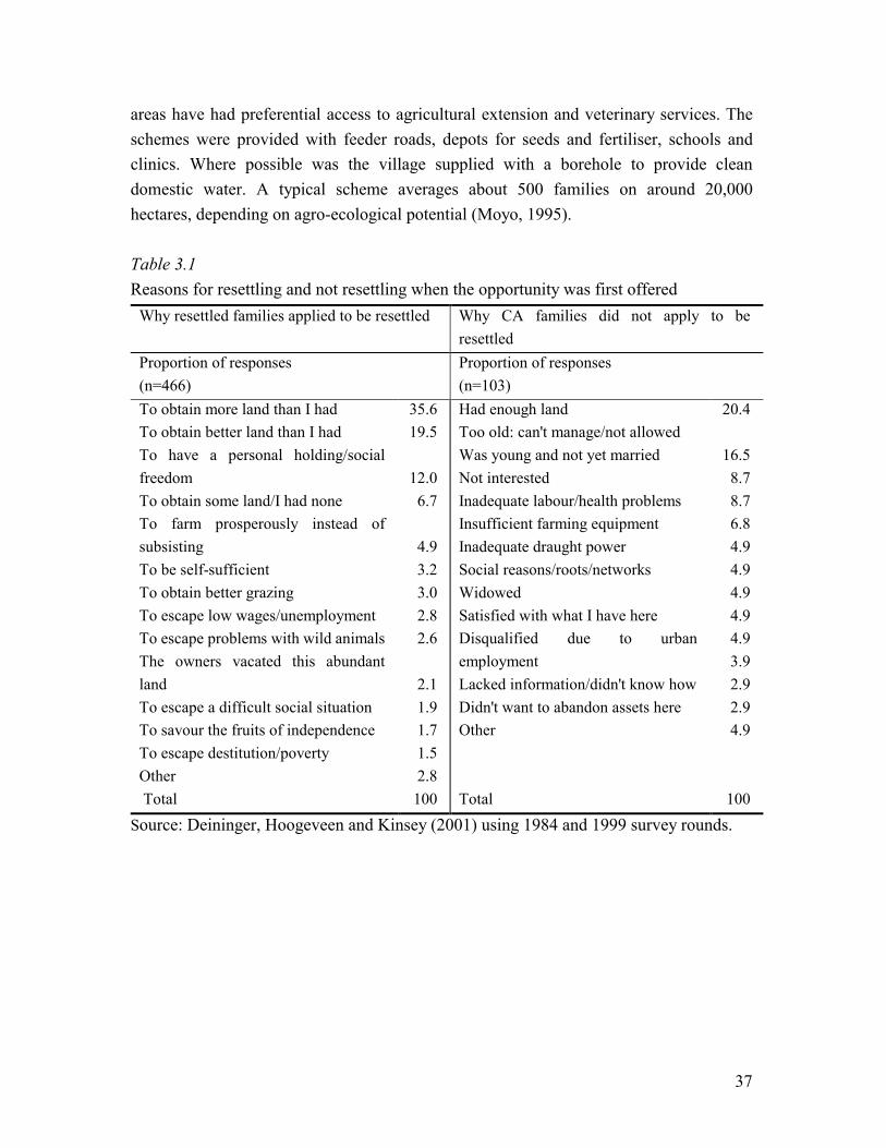
37

areas have had preferential access to agricultural extension and veterinary services. The schemes were provided with feeder roads, depots for seeds and fertiliser, schools and clinics. Where possible was the village supplied with a borehole to provide clean domestic water. A typical scheme averages about 500 families on around 20,000 hectares, depending on agro-ecological potential (Moyo, 1995). Table 3.1 Reasons for resettling and not resettling when the opportunity was first offered

Why resettled families applied to be resettled Why CA families did not apply to be resettled

Proportion of responses (n=466)

Proportion of responses (n=103)

To obtain more land than I had To obtain better land than I had To have a personal holding/social freedom To obtain some land/I had none To farm prosperously instead of subsisting To be self-sufficient To obtain better grazing To escape low wages/unemployment To escape problems with wild animals The owners vacated this abundant land To escape a difficult social situation To savour the fruits of independence To escape destitution/poverty Other Total

35.6 19.5

12.0 6.7

4.9 3.2 3.0 2.8 2.6

2.1 1.9 1.7 1.5 2.8

100

Had enough land Too old: can't manage/not allowed Was young and not yet married Not interested Inadequate labour/health problems Insufficient farming equipment Inadequate draught power Social reasons/roots/networks Widowed Satisfied with what I have here Disqualified due to urban employment Lacked information/didn't know how Didn't want to abandon assets here Other Total

20.4

16.5 8.7 8.7 6.8 4.9 4.9 4.9 4.9 4.9 3.9 2.9 2.9 4.9

100 Source: Deininger, Hoogeveen and Kinsey (2001) using 1984 and 1999 survey rounds.

38

3.3 Sampling Issues In Zimbabwe five zones of different agro-ecological potential are distinguished. These zones, called national regions (NR), are labelled I to V. The areas labelled NR I are those with the greatest agricultural potential; areas labelled as NR V are those with the least potential. To reflect differing physical environments, Kinsey intended to select one resettlement scheme in each agro-ecological zone, but in practice this turned out to be not possible. By the time surveying started in 1983, no households had been resettled in NR I while households in NR V could not be included because of the poor security situation in Matabeleland (in Southern Zimbabwe where this agro-ecological zone is mostly located) at that time. Thus neither of Zimbabwe�s regions of highest and lowest agricultural potential is represented in the sample. The characteristics of the zones included in the survey are described in Box 3.1. Box 3.1 Natural Regions represented in the survey Natural Region II (NR II): This region is characterised by intensive farming. Rainfall is moderately high (750-1000 mm), but is confined to the summer months (October-April). Two subregions have been identified within this region. Subregion IIA receives an average of at least 18 rainy pentads per season and is normally reliable, rarely experiencing severe dry spell during the rainy season. The region is suitable for intensive crop or livestock farming systems. Sub-region IIB receives an average of 16-18 pentads per season, but is subject to severe dry rainy seasons. Crop yields are affected in certain years, but not frequently enough to justify shifting cropping practices away from intensive farming systems. Natural Region III (NR III): Semi-intensive farming is practised in this region. Precipitation is moderate (650-800 mm), but severe mid-season dry spells and high temperatures limit its effectiveness. Conditions for growing maize, tobacco and cotton production are marginal. Livestock production, fodder crop farming and the farming of cash crops with good moisture retention are the suitable farming systems in the regions. Natural Region IV (NR IV): This is a semi-extensive farming region. Rainfall is relatively low (450-600 mm) and is subject to periodic seasonal droughts and severe dry spells during the rainy season. Low and uncertain rainfall male cash cropping risky except for drought-resistant crops and soils with better water retention. Farming systems are suited to livestock production with some intensification possible with drought resistant fodder crops.

Source: adapted from Moyo, 1995. Random sampling was used to select villages within each scheme, and in each selected village a census was attempted of all resident households. In Mpfurudzi, in NR II, 230 households located in nine villages were interviewed. In Sengezi in NR III, 100 households in five villages were selected while the sample comprises 70 households in

39

Mutanda, NR IV, located in seven villages. In 1997 a group of communal households was added to the original survey to serve as counterfactual to the land reform experience. In each natural region the two communal villages were selected that had supplied the largest number of households to the survey. In each selected village, 25 households were interviewed, so that a total of 150 households were added.12 Table 3.2 Selected characteristics of the three resettlement schemes included in the data set

Scheme Mpfurudzi Sengezi Mutanda Province Mashonaland

Central Mashonaland East

Manicaland

District Shamva Wedza Makoni Natural Region IIb / III IIb / III III / IV Area (sq. km) 345 84 439 Year Settlement officially began 1980 1981 1981 Number of Settlement Villages 18 8 29 Number of settler households 563 289 575 Mean area available per household (ha)

61 29 76

Source: adapted from Kinsey, 1998. From the way the sample was drawn it follows that the three different natural regions should be considered as strata from which the villages were drawn (the clusters). The presence of strata and clusters has consequences for standard errors when determining summary statistics or while generating regression output. Its impact can be clarified as follows. Suppose households in natural region II possess on average more livestock than those in natural region IV and let the aim be to determine the number of livestock of a resettled household and the standard error of the estimated mean. If several surveys would be held, each using a different sample of the population to determine the sample variation, then the fraction of households in each of the strata is likely to differ. This increases sample variation. The effect of stratification is to fix the number of households in each stratum, in this case each natural region, so as to avoid sample variation that follows from having different fractions of observations in each natural region. The 12 In 1999 the survey has been expanded further to include all households in all the villages covered. In this way an extra 180 household were added. These households are not included in any of the analyses in this thesis.

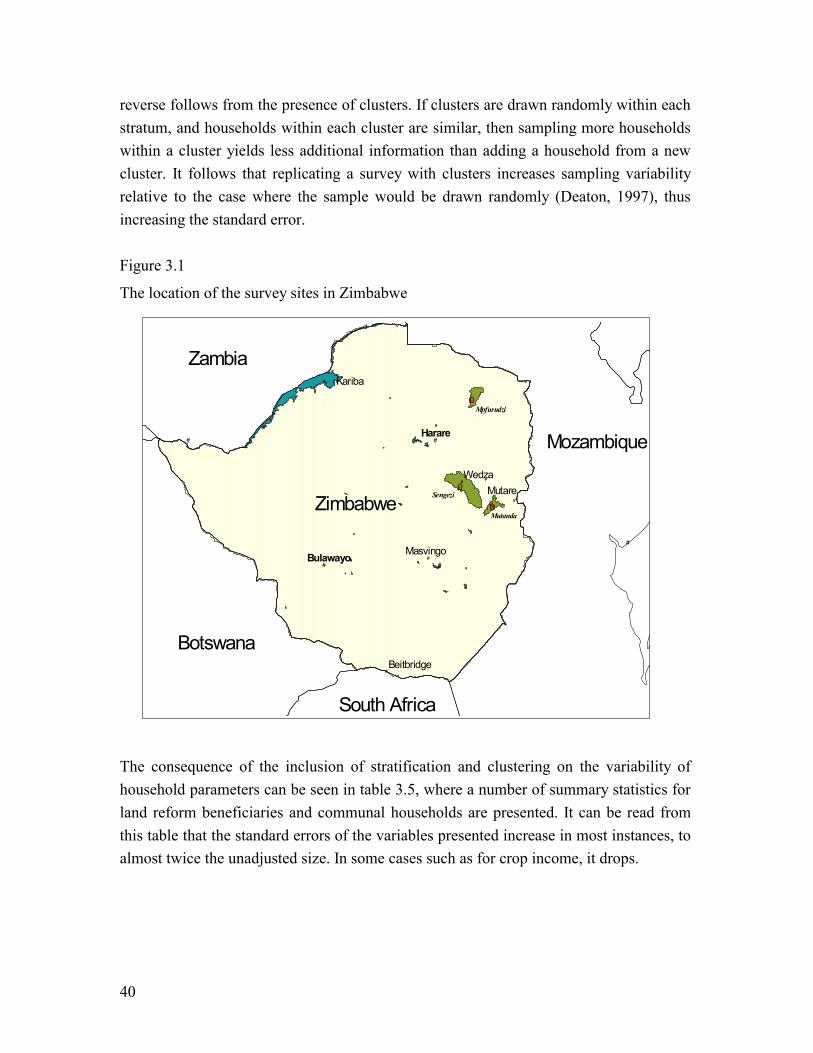
40

reverse follows from the presence of clusters. If clusters are drawn randomly within each stratum, and households within each cluster are similar, then sampling more households within a cluster yields less additional information than adding a household from a new cluster. It follows that replicating a survey with clusters increases sampling variability relative to the case where the sample would be drawn randomly (Deaton, 1997), thus increasing the standard error. Figure 3.1

The location of the survey sites in Zimbabwe

#

#

#

#

#

#

#

#

#

South Africa

Zambia

Mozambique

Botswana

Zimbabwe

Harare

Bulawayo

Mpfurudzi

Sengezi

Mutanda

ÊÚ

ÊÚ

ÊÚ

Wedza

Kariba

Mutare

Masvingo

Beitbridge

The consequence of the inclusion of stratification and clustering on the variability of household parameters can be seen in table 3.5, where a number of summary statistics for land reform beneficiaries and communal households are presented. It can be read from this table that the standard errors of the variables presented increase in most instances, to almost twice the unadjusted size. In some cases such as for crop income, it drops.

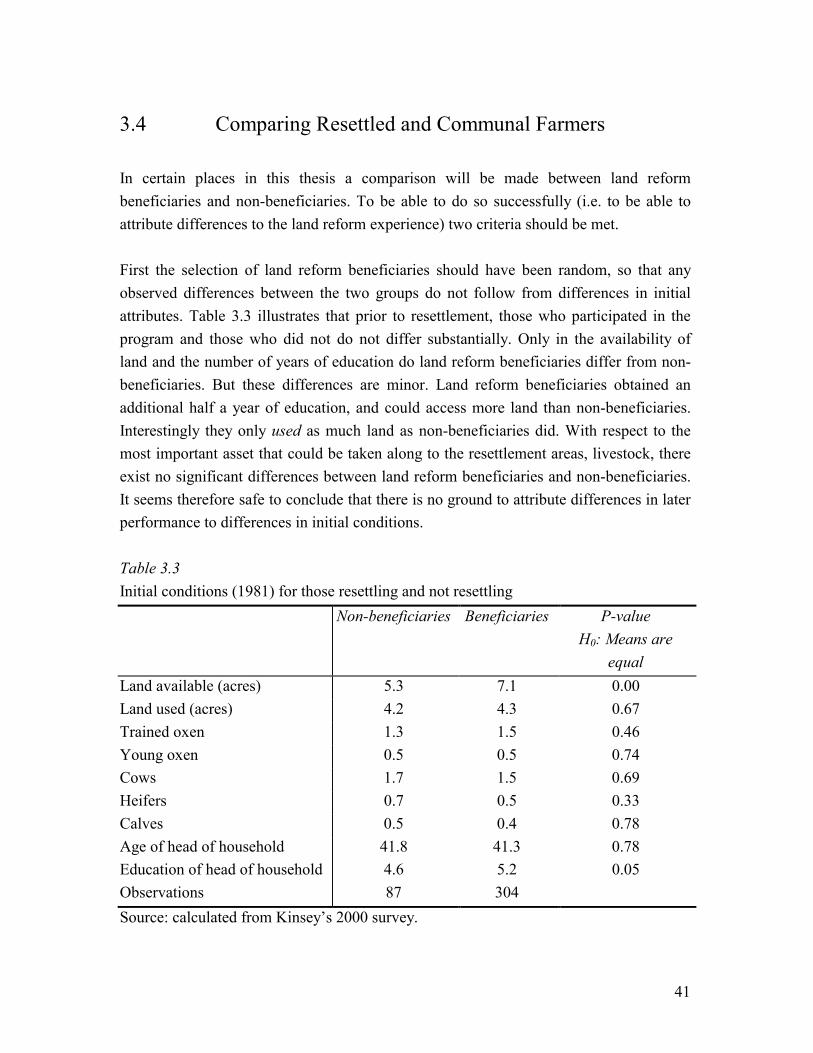
41

3.4 Comparing Resettled and Communal Farmers In certain places in this thesis a comparison will be made between land reform beneficiaries and non-beneficiaries. To be able to do so successfully (i.e. to be able to attribute differences to the land reform experience) two criteria should be met. First the selection of land reform beneficiaries should have been random, so that any observed differences between the two groups do not follow from differences in initial attributes. Table 3.3 illustrates that prior to resettlement, those who participated in the program and those who did not do not differ substantially. Only in the availability of land and the number of years of education do land reform beneficiaries differ from non-beneficiaries. But these differences are minor. Land reform beneficiaries obtained an additional half a year of education, and could access more land than non-beneficiaries. Interestingly they only used as much land as non-beneficiaries did. With respect to the most important asset that could be taken along to the resettlement areas, livestock, there exist no significant differences between land reform beneficiaries and non-beneficiaries. It seems therefore safe to conclude that there is no ground to attribute differences in later performance to differences in initial conditions. Table 3.3 Initial conditions (1981) for those resettling and not resettling Non-beneficiaries Beneficiaries P-value

H0: Means are equal

Land available (acres) 5.3 7.1 0.00 Land used (acres) 4.2 4.3 0.67 Trained oxen 1.3 1.5 0.46 Young oxen 0.5 0.5 0.74 Cows 1.7 1.5 0.69 Heifers 0.7 0.5 0.33 Calves 0.5 0.4 0.78 Age of head of household 41.8 41.3 0.78 Education of head of household 4.6 5.2 0.05 Observations 87 304 Source: calculated from Kinsey�s 2000 survey.

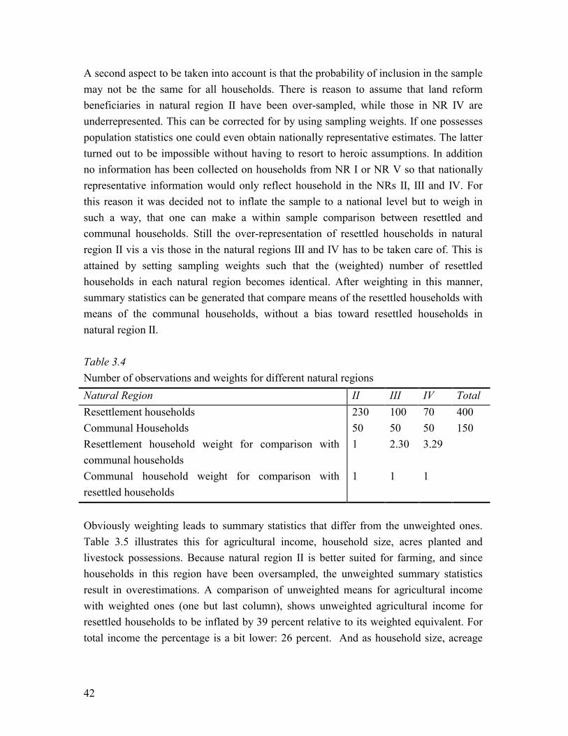
42

A second aspect to be taken into account is that the probability of inclusion in the sample may not be the same for all households. There is reason to assume that land reform beneficiaries in natural region II have been over-sampled, while those in NR IV are underrepresented. This can be corrected for by using sampling weights. If one possesses population statistics one could even obtain nationally representative estimates. The latter turned out to be impossible without having to resort to heroic assumptions. In addition no information has been collected on households from NR I or NR V so that nationally representative information would only reflect household in the NRs II, III and IV. For this reason it was decided not to inflate the sample to a national level but to weigh in such a way, that one can make a within sample comparison between resettled and communal households. Still the over-representation of resettled households in natural region II vis a vis those in the natural regions III and IV has to be taken care of. This is attained by setting sampling weights such that the (weighted) number of resettled households in each natural region becomes identical. After weighting in this manner, summary statistics can be generated that compare means of the resettled households with means of the communal households, without a bias toward resettled households in natural region II. Table 3.4 Number of observations and weights for different natural regions Natural Region II III IV Total Resettlement households 230 100 70 400 Communal Households 50 50 50 150 Resettlement household weight for comparison with communal households

1 2.30 3.29

Communal household weight for comparison with resettled households

1 1 1

Obviously weighting leads to summary statistics that differ from the unweighted ones. Table 3.5 illustrates this for agricultural income, household size, acres planted and livestock possessions. Because natural region II is better suited for farming, and since households in this region have been oversampled, the unweighted summary statistics result in overestimations. A comparison of unweighted means for agricultural income with weighted ones (one but last column), shows unweighted agricultural income for resettled households to be inflated by 39 percent relative to its weighted equivalent. For total income the percentage is a bit lower: 26 percent. And as household size, acreage

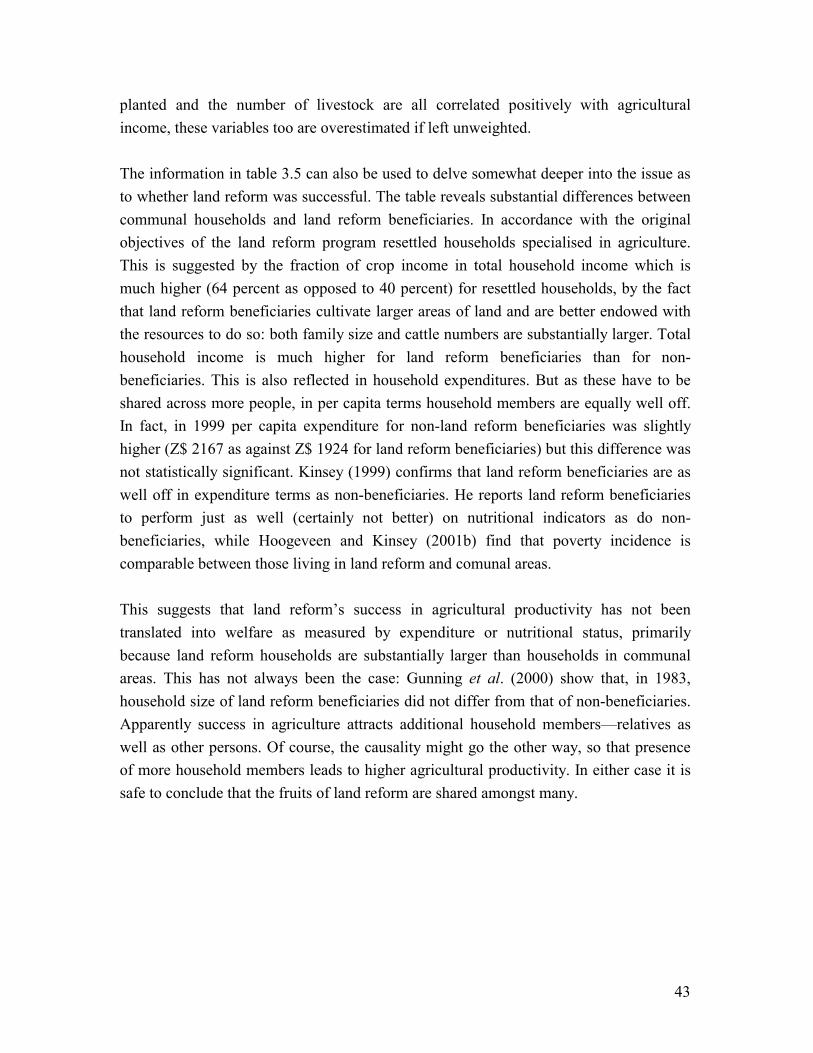
43

planted and the number of livestock are all correlated positively with agricultural income, these variables too are overestimated if left unweighted. The information in table 3.5 can also be used to delve somewhat deeper into the issue as to whether land reform was successful. The table reveals substantial differences between communal households and land reform beneficiaries. In accordance with the original objectives of the land reform program resettled households specialised in agriculture. This is suggested by the fraction of crop income in total household income which is much higher (64 percent as opposed to 40 percent) for resettled households, by the fact that land reform beneficiaries cultivate larger areas of land and are better endowed with the resources to do so: both family size and cattle numbers are substantially larger. Total household income is much higher for land reform beneficiaries than for non-beneficiaries. This is also reflected in household expenditures. But as these have to be shared across more people, in per capita terms household members are equally well off. In fact, in 1999 per capita expenditure for non-land reform beneficiaries was slightly higher (Z$ 2167 as against Z$ 1924 for land reform beneficiaries) but this difference was not statistically significant. Kinsey (1999) confirms that land reform beneficiaries are as well off in expenditure terms as non-beneficiaries. He reports land reform beneficiaries to perform just as well (certainly not better) on nutritional indicators as do non-beneficiaries, while Hoogeveen and Kinsey (2001b) find that poverty incidence is comparable between those living in land reform and comunal areas. This suggests that land reform�s success in agricultural productivity has not been translated into welfare as measured by expenditure or nutritional status, primarily because land reform households are substantially larger than households in communal areas. This has not always been the case: Gunning et al. (2000) show that, in 1983, household size of land reform beneficiaries did not differ from that of non-beneficiaries. Apparently success in agriculture attracts additional household members�relatives as well as other persons. Of course, the causality might go the other way, so that presence of more household members leads to higher agricultural productivity. In either case it is safe to conclude that the fruits of land reform are shared amongst many.

44

Table 3.5 Differences between resettled and communal households and the importance of weighting, stratification and clustering, using 1999 data (1997/98 season) Mean std error 1 mean std error

Unweighted Unstratified Unclustered

Weighted 2

Stratified Clustered

Gross income3 Resettled 23560 1140 18652 1497 in Z$ Communal 8592 865 8592 519 Sales value of crops Resettled 16365 1680 11813 1352 in Z$ Communal 3432 415 3432 702 Expenditures4 Resettled 19285 1035 18466 832 in Z$ Communal 14087 564 14087 653 Household size Resettled 10.3 0.43 9.6 0.36

Communal 6.5 0.27 6.5 0.48 Acres planted Resettled 8.2 0.31 7.9 0.36

Communal 4.3 0.21 4.3 0.28 Head of cattle5 Resettled 8.7 0.69 8.5 0.64

Communal 4.9 0.40 4.9 0.62

1 The standard error is determined as the standard deviation divided by the square root of the number of observations (380 land reform beneficiaries and 140 communal households).

2 Weights are from table 3.2. 3 Gross income consists of gross crop income, gross income entrepreneurial activities,

gross income from female activities (gardening mostly), income from off farm employment, income from public transfers, income from remittances, gross income from .

4 Expenditures comprise of food expenditures and expenditures on consumer durables. Not included are expenses for clothing, transport, housing, education, ceremonies or medical expenses.

5 Head of cattle comprises heifers, oxen, bulls and cows. Source: calculated from Kinsey�s 1999 survey

Land reform beneficiaries are obviously not representative for Zimbabwe�s communal farmers. The atypical specialisation in agriculture also has its advantages as it makes them fit remarkably well in Binswanger�s and McIntire�s (1987) characterisation of what constitutes a typical farmer in a land abundant environment, namely a person who, apart

45

from relying on agriculture as his prime source of income, operates in an environment with absent regular output and labour markets, and the non-existence of a landless labour class, with minimal access to credit markets and professional money lenders, who lives in an environment with livestock tenancy but no tenancy in land and where livestock is an important asset for production and an insurance substitute.

3.5 Making Comparisons over Time

One of Kinsey�s motivations to create a panel data set was to be able to study over time the dynamics of households as they took advantage of the opportunities offered by resettlement. To facilitate this, the questionnaires comprise a sizeable core of questions (including assets, expenditure, income and household composition) that remained mostly unchanged in the course of time. This holds especially for the interviews held since 1992. It is on these years this thesis focuses. Another aspect favourable for comparisons over time is that there is little sample attrition. Approximately 85 percent of households interviewed in 1983-84 are still in the sample. There is no systematic pattern to the few households dropping out. Some were inadvertently dropped during the re-surveys, a few disintegrated (such as those where all adults died) and a small number were evicted by government officials responsible for overseeing these schemes. An entirely different issue is that not individual households are tracked in the Kinsey panel, but the land usufructed by the original settlers. Survey teams visit residential stands and carry out an interview even if the original plot-holder has died and his permits passed on to his/her heirs. From the perspective of the original household, one might consider it to be dissolved and it would seem more appropriate to speak of a new household altogether. From the perspective of sample representativiness this procedure does have certain advantages however, because it permits a continuous inflow of new households, so that the sample does not just follow a cohort of households over time. It also follows that if one is especially interested in the cohort, precautions have to be taken. In table 3.6 the yearly changes in the head of household are presented for each of the years since 1992. Considering that the panel has been in operation for almost 20 years it has remained remarkably stable.

46

Table 3.6 Number of households experiencing a change in the head of household Survey year 1993 1994 1995 1996 1997 1998 1999 Resettlement - 4 2 4 12 7 6 Communal - 2 0 Source: determined from Kinsey�s 1993-1999 surveys An additional point of concern is Zimbabwe�s inflation rates, implying that monetary variables cannot be compared over time without taking into consideration price changes. Consider table 3.7 for instance. It illustrates that even over a relatively short period, livestock prices increased substantially. In fact, almost all prices doubled over between 1997 and 1999 and tripled between 1995 and 1999.

To deal with this issue, obtaining a consumer price index is of importance. Unfortunately, the available price index compiled by Zimbabwe�s Statistical Office (CSO) is for urban households and therefore of less relevance for rural households. But ever since 1994 price information on a large number of food items and consumer durables is available from the questionnaires and these can serve as basis for the construction of a rural CPI. In table 3.8 prices for these items are presented.

Table 3.7

Evolution of median livestock prices

Survey year 1995 1996 1997 1998 1999Cow 1200 1500 1800 2600 3500Heifer 1000 1200 1500 2000 3000

Trained oxen

1800 2000 2500 4000 4500

Young oxen 1000 1200 1600 2000 3000Bull 1500 2000 2000 3000 3500Goat 85 120 150 200 300 Source: calculated using Kinsey�s 1995-1999 surveys

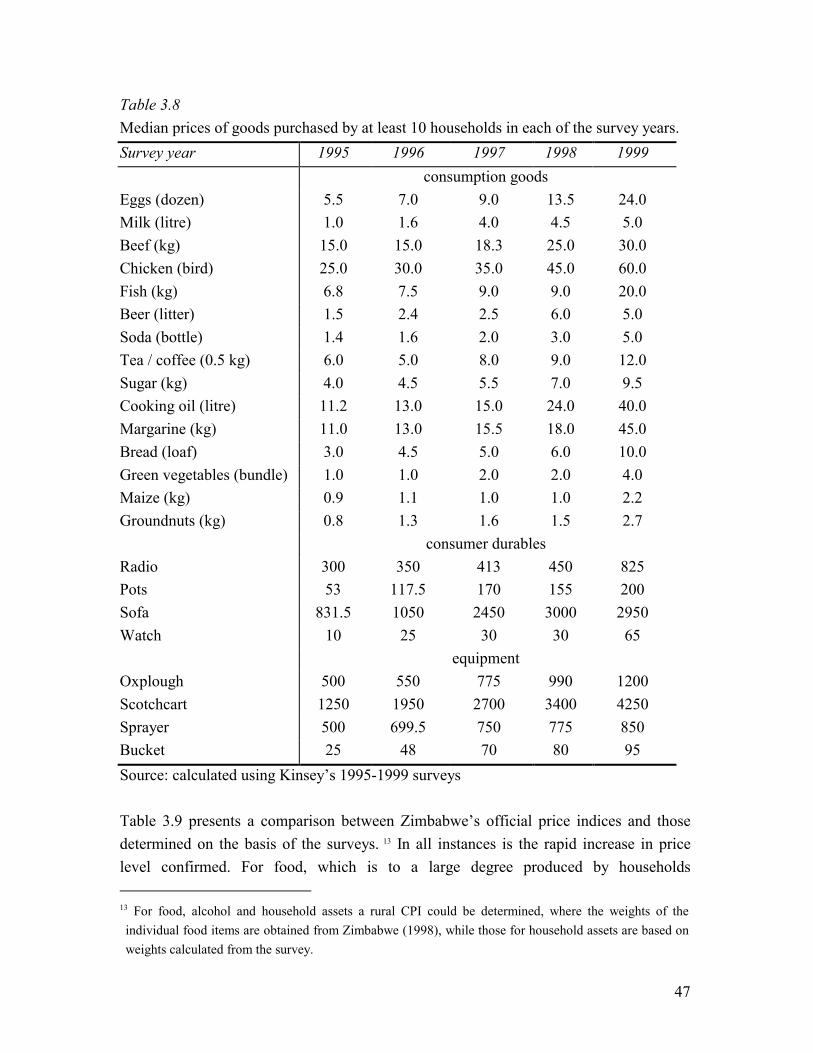
47

Table 3.8 Median prices of goods purchased by at least 10 households in each of the survey years. Survey year 1995 1996 1997 1998 1999 consumption goods Eggs (dozen) 5.5 7.0 9.0 13.5 24.0 Milk (litre) 1.0 1.6 4.0 4.5 5.0 Beef (kg) 15.0 15.0 18.3 25.0 30.0 Chicken (bird) 25.0 30.0 35.0 45.0 60.0 Fish (kg) 6.8 7.5 9.0 9.0 20.0 Beer (litter) 1.5 2.4 2.5 6.0 5.0 Soda (bottle) 1.4 1.6 2.0 3.0 5.0 Tea / coffee (0.5 kg) 6.0 5.0 8.0 9.0 12.0 Sugar (kg) 4.0 4.5 5.5 7.0 9.5 Cooking oil (litre) 11.2 13.0 15.0 24.0 40.0 Margarine (kg) 11.0 13.0 15.5 18.0 45.0 Bread (loaf) 3.0 4.5 5.0 6.0 10.0 Green vegetables (bundle) 1.0 1.0 2.0 2.0 4.0 Maize (kg) 0.9 1.1 1.0 1.0 2.2 Groundnuts (kg) 0.8 1.3 1.6 1.5 2.7 consumer durables Radio 300 350 413 450 825 Pots 53 117.5 170 155 200 Sofa 831.5 1050 2450 3000 2950 Watch 10 25 30 30 65 equipment Oxplough 500 550 775 990 1200 Scotchcart 1250 1950 2700 3400 4250 Sprayer 500 699.5 750 775 850 Bucket 25 48 70 80 95 Source: calculated using Kinsey�s 1995-1999 surveys Table 3.9 presents a comparison between Zimbabwe�s official price indices and those determined on the basis of the surveys. 13 In all instances is the rapid increase in price level confirmed. For food, which is to a large degree produced by households 13 For food, alcohol and household assets a rural CPI could be determined, where the weights of the individual food items are obtained from Zimbabwe (1998), while those for household assets are based on weights calculated from the survey.

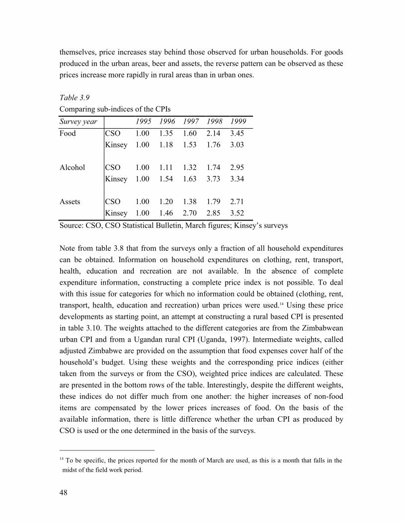
48

themselves, price increases stay behind those observed for urban households. For goods produced in the urban areas, beer and assets, the reverse pattern can be observed as these prices increase more rapidly in rural areas than in urban ones. Table 3.9 Comparing sub-indices of the CPIs Survey year 1995 1996 1997 1998 1999 Food CSO 1.00 1.35 1.60 2.14 3.45 Kinsey 1.00 1.18 1.53 1.76 3.03 Alcohol CSO 1.00 1.11 1.32 1.74 2.95 Kinsey 1.00 1.54 1.63 3.73 3.34 Assets CSO 1.00 1.20 1.38 1.79 2.71 Kinsey 1.00 1.46 2.70 2.85 3.52 Source: CSO, CSO Statistical Bulletin, March figures; Kinsey�s surveys Note from table 3.8 that from the surveys only a fraction of all household expenditures can be obtained. Information on household expenditures on clothing, rent, transport, health, education and recreation are not available. In the absence of complete expenditure information, constructing a complete price index is not possible. To deal with this issue for categories for which no information could be obtained (clothing, rent, transport, health, education and recreation) urban prices were used.14 Using these price developments as starting point, an attempt at constructing a rural based CPI is presented in table 3.10. The weights attached to the different categories are from the Zimbabwean urban CPI and from a Ugandan rural CPI (Uganda, 1997). Intermediate weights, called adjusted Zimbabwe are provided on the assumption that food expenses cover half of the household�s budget. Using these weights and the corresponding price indices (either taken from the surveys or from the CSO), weighted price indices are calculated. These are presented in the bottom rows of the table. Interestingly, despite the different weights, these indices do not differ much from one another: the higher increases of non-food items are compensated by the lower prices increases of food. On the basis of the available information, there is little difference whether the urban CPI as produced by CSO is used or the one determined in the basis of the surveys.

14 To be specific, the prices reported for the month of March are used, as this is a month that falls in the midst of the field work period.

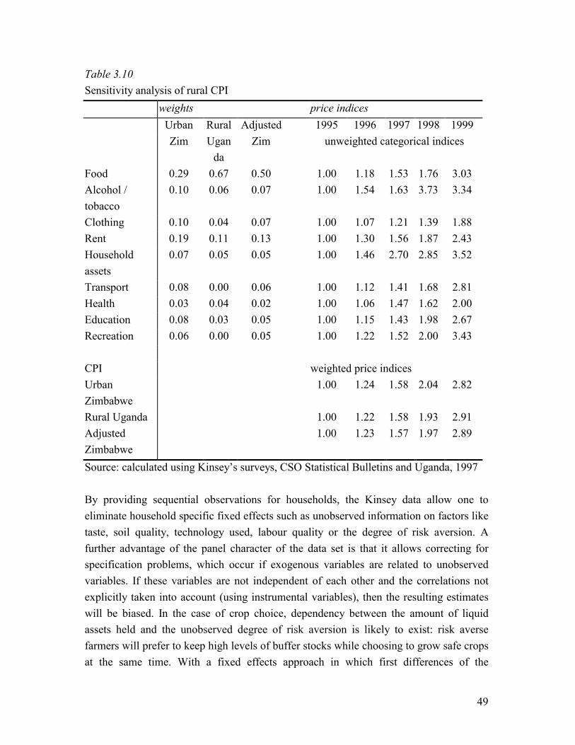
49

Table 3.10 Sensitivity analysis of rural CPI weights price indices Urban Rural Adjusted 1995 1996 1997 1998 1999 Zim Ugan

da Zim unweighted categorical indices

Food 0.29 0.67 0.50 1.00 1.18 1.53 1.76 3.03 Alcohol / tobacco

0.10 0.06 0.07 1.00 1.54 1.63 3.73 3.34

Clothing 0.10 0.04 0.07 1.00 1.07 1.21 1.39 1.88 Rent 0.19 0.11 0.13 1.00 1.30 1.56 1.87 2.43 Household assets

0.07 0.05 0.05 1.00 1.46 2.70 2.85 3.52

Transport 0.08 0.00 0.06 1.00 1.12 1.41 1.68 2.81 Health 0.03 0.04 0.02 1.00 1.06 1.47 1.62 2.00 Education 0.08 0.03 0.05 1.00 1.15 1.43 1.98 2.67 Recreation 0.06 0.00 0.05 1.00 1.22 1.52 2.00 3.43 CPI weighted price indices Urban Zimbabwe

1.00 1.24 1.58 2.04 2.82

Rural Uganda 1.00 1.22 1.58 1.93 2.91 Adjusted Zimbabwe

1.00 1.23 1.57 1.97 2.89

Source: calculated using Kinsey�s surveys, CSO Statistical Bulletins and Uganda, 1997 By providing sequential observations for households, the Kinsey data allow one to eliminate household specific fixed effects such as unobserved information on factors like taste, soil quality, technology used, labour quality or the degree of risk aversion. A further advantage of the panel character of the data set is that it allows correcting for specification problems, which occur if exogenous variables are related to unobserved variables. If these variables are not independent of each other and the correlations not explicitly taken into account (using instrumental variables), then the resulting estimates will be biased. In the case of crop choice, dependency between the amount of liquid assets held and the unobserved degree of risk aversion is likely to exist: risk averse farmers will prefer to keep high levels of buffer stocks while choosing to grow safe crops at the same time. With a fixed effects approach in which first differences of the

50

individual observations over time are taken, the influence of the unobserved (but constant) variable cancels out and unbiased estimates are obtained (Hsiao, 1985). But the use of panel data comes with its own problems. Suppose, for instance, that the data are measured with error. If this error is uncorrelated with the true value then the variance of the measured x is the variance of the true x, plus the variance of the measurement error (3.1)

)var()var()var( *ititit xx ε+= (3.1)

where εit is a mean zero measurement error. Let�s assume for convenience that the error variance is the same for both periods. It then follows that if the observations are differenced over time, one gets:

)1)(var(2)var()var( * ρε −+∆=∆ ititit xx (3.2)

where ρ is the correlation between the errors in the two periods. It follows that if x changes only slowly over time that the variance of true changes is smaller than the variance for levels in equation (3.1). On the other hand, the variance of measurement error in changes will be double that in levels if ρ = 0 (3.2), and will be increased by differencing unless ρ > 0. There is no general result here, but there will be many cases in household survey data where the variance of the measured changes will be dominated by measurement error, even when the measurement of the levels is relatively accurate (Deaton, 1997). Table 3.11 provides an example of how taking first differences increases the magnitude of the standard error relative its parameter. For instance, standard errors for gross income or crop sales are smaller in first differences, but as percentage of the reported mean they are substantially larger. In most cases is the absolute value of the differenced standard error smaller than that for levels. But even this is not true in all cases, as is illustrated by communal cattle ownership.

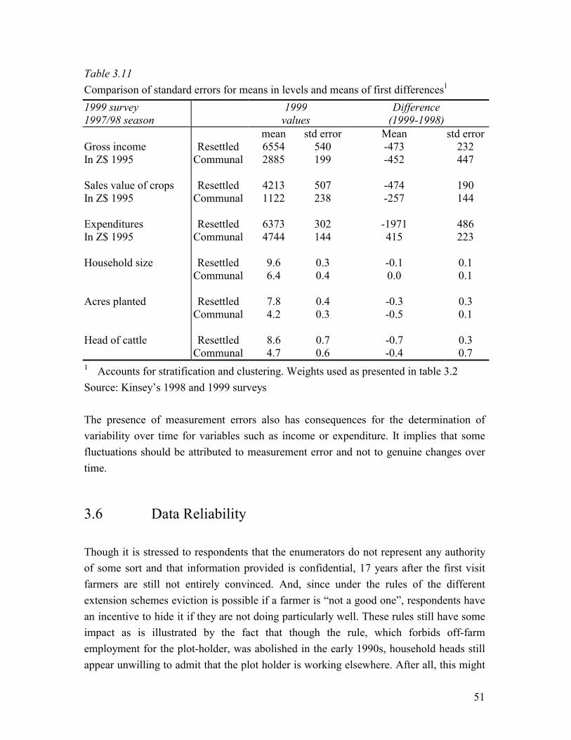
51

Table 3.11 Comparison of standard errors for means in levels and means of first differences1 1999 survey 1997/98 season

1999 values

Difference (1999-1998)

mean std error Mean std errorGross income Resettled 6554 540 -473 232 In Z$ 1995 Communal 2885 199 -452 447 Sales value of crops Resettled 4213 507 -474 190 In Z$ 1995 Communal 1122 238 -257 144 Expenditures Resettled 6373 302 -1971 486 In Z$ 1995 Communal 4744 144 415 223 Household size Resettled 9.6 0.3 -0.1 0.1

Communal 6.4 0.4 0.0 0.1 Acres planted Resettled 7.8 0.4 -0.3 0.3

Communal 4.2 0.3 -0.5 0.1 Head of cattle Resettled 8.6 0.7 -0.7 0.3

Communal 4.7 0.6 -0.4 0.7

1 Accounts for stratification and clustering. Weights used as presented in table 3.2 Source: Kinsey�s 1998 and 1999 surveys The presence of measurement errors also has consequences for the determination of variability over time for variables such as income or expenditure. It implies that some fluctuations should be attributed to measurement error and not to genuine changes over time.

3.6 Data Reliability Though it is stressed to respondents that the enumerators do not represent any authority of some sort and that information provided is confidential, 17 years after the first visit farmers are still not entirely convinced. And, since under the rules of the different extension schemes eviction is possible if a farmer is �not a good one�, respondents have an incentive to hide it if they are not doing particularly well. These rules still have some impact as is illustrated by the fact that though the rule, which forbids off-farm employment for the plot-holder, was abolished in the early 1990s, household heads still appear unwilling to admit that the plot holder is working elsewhere. After all, this might

52

still be interpreted as a lack of interest in one�s own fields or considered a signal that the household is not doing particularly well. But the degree of mistrust should not be exaggerated. By returning year after year, a certain mutual understanding has developed between interviewed and enumerators and in some cases, data reliability is enhanced by the fact that farmers expect a return visit. Some farmers keep the sales slips for their crops for instance and present them to the enumerators when the crop section of the questionnaire is dealt with. That farmers trust the enumerators is illustrated by the fact that 39 percent of the sampled households indicated in 1999 that they possessed more than eight head of cattle, the maximum allowed by their permit. Nearly ten percent of households even claimed to possess more than 20 beasts. That there exists a certain degree of trust between enumerators and farmers is also illustrated by the answers given to questions on land rental and clearance of new fields. One could suspect that asking for rental transactions arouses suspicion as, formally at least, land transactions are not allowed in the resettled areas. Nonetheless, in 1999, nearly ten percent of the households claimed to cultivate an area that exceeded the 12 acres allotted to them by the resettlement authorities, while two percent of the households said that they were renting in land. Those households (ten percent) who indicated to have cleared land (something equally forbidden) make up the difference.15 Various stages of checking the information after it has been collected enhanced data reliability. First the enumerators, who visit the households in teams of two but who work independently (interviewing husband and wife separately), check each other�s sections. Next enumerator teams check each other�s work. The field supervisor carries out a last check before a data analyst who performs a final check enters the data in a computer. Mistakes and inconsistencies found are corrected, either by referring back to the enumerators or, if need arises, by revisiting the household. Finally, the fact that there is a core set of enumerators that participated each year facilitates consistency in the collection of the data and eases collaboration with officials. Despite the care exercised in data collection certain variables remain problematic. Farmers probably underreport their cash holdings for instance out of fear for theft. Not only money disappears. Cattle, goats and poultry all get stolen. Telling is the story of the farmer who discovered after an absence of six months due to illness that all his fencing had gone. Avoiding opportunistic relatives might be another reason not to be clear about 15 In a separate survey held under a sub-sample of 50 farmers included in the Kinsey sample, Loef (2000), finds a comparable percentage of households that borrowed or extended their land: 13.4 percent.

53

the amount of cash available at home. All this calls for caution in revealing ones liquid assets. This secrecy appears to be confined to specific goods however and respondents are very open about their possessions of farm equipment and livestock assets. As always obtaining reliable estimates for income and expenditures remains problematic. Income is obtained from many different sources and registered in several places in the questionnaire. Being semi-subsistence farmers, not all crops are sold on the market so that solutions need to be found in attributing values to physical quantities. Crop and entrepreneurial income are recorded in gross terms as net figures could not be obtained. Being registered in different sections of the questionnaires, double counting can not always be avoided, nor the fact that certain sources of income may not be recorded at all. Especially for communal households this is a concern, as can be concluded from table 3.12, where one finds for resettled households expenditures to be relatively close to gross income (though there is no a priori reason why this should be the case). This is much less the case for communal households. If one adds to this that in per capita terms the value of livestock possessions (this is the main store of wealth) is comparable for land reform beneficiaries and communal households, it suggests underreporting of gross income for communal households. After all, if per capita expenditure is comparable and so are the accumulated savings then per capita incomes should not diverge too much either. A priori there is reason to suspect that measurement error are more acute in determining income earned by communal households because they obtain a much larger fraction of their income from off-farm sources. Since the questionnaires were designed to inform about land reform beneficiaries who � until 1992 forced by regulations, were primarily involved in agriculture, capturing information on off-farm activities never received fullest attention. The general approach followed in this thesis is that most weight is attached to gross income for resettled households as this is believed to be most complete. Where relevant it is compared to gross incomes for communal households though it is believed to be underreported. Expenditure information is used as a crosscheck.

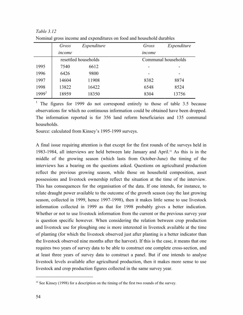
54

Table 3.12 Nominal gross income and expenditures on food and household durables Gross

income Expenditure Gross

income Expenditure

resettled households Communal households 1995 7540 6612 - - 1996 6426 9800 - - 1997 14604 11908 8382 8874 1998 13822 16422 6548 8524 19991 18959 18350 8304 13756

1 The figures for 1999 do not correspond entirely to those of table 3.5 because observations for which no continuous information could be obtained have been dropped. The information reported is for 356 land reform beneficiaries and 135 communal households. Source: calculated from Kinsey�s 1995-1999 surveys. A final issue requiring attention is that except for the first rounds of the surveys held in 1983-1984, all interviews are held between late January and April.16 As this is in the middle of the growing season (which lasts from October-June) the timing of the interviews has a bearing on the questions asked. Questions on agricultural production reflect the previous growing season, while those on household composition, asset possessions and livestock ownership reflect the situation at the time of the interview. This has consequences for the organisation of the data. If one intends, for instance, to relate draught power available to the outcome of the growth season (say the last growing season, collected in 1999, hence 1997-1998), then it makes little sense to use livestock information collected in 1999 as that for 1998 probably gives a better indication. Whether or not to use livestock information from the current or the previous survey year is question specific however. When considering the relation between crop production and livestock use for ploughing one is more interested in livestock available at the time of planting (for which the livestock observed just after planting is a better indicator than the livestock observed nine months after the harvest). If this is the case, it means that one requires two years of survey data to be able to construct one complete cross-section, and at least three years of survey data to construct a panel. But if one intends to analyse livestock levels available after agricultural production, then it makes more sense to use livestock and crop production figures collected in the same survey year.

16 See Kinsey (1998) for a description on the timing of the first two rounds of the survey.

55

3.7 Conclusion The data for this thesis are from a unique African panel that comprises (i) a long term, continuous panel of land reform beneficiaries (from 1992 till 1999) and (ii) a shorter panel (1997-1999) for non-land reform beneficiaries. The long panel for resettled households provides a great opportunity to study long-term developmental issues like the ones this thesis deals with: how rural households deal with risk and insurance. The resettled households for whom most information is available can not be considered representative for Zimbabwe�s communal farmers. As beneficiaries of the land reform program these farmers are atypical, either in the quality, and the quantity of land they possess, the access to services and infrastructure and their lack of access to off farm activities, their wealth and family size and the restrictions applying to them. This does not imply that this group of farmers can not inform us about risk and insurance by smallholder farmers. In fact one may argue that they are especially suited to serve this objective as the characteristics of these farmers are such that they fit remarkably well in Binswanger�s and McIntire�s (1987) characterisation of what constitutes a typical farmer in a land abundant environment. The inclusion of a shorter panel for communal households allows making comparisons between those who benefited from land reform and those who did not, especially as indications for selection bias are weak (though not entirely absent). This allows considering how land reform beneficiaries fare relative to non-beneficiaries. In terms of household income, expenditure and asset ownership resettled households are much better off than their communal counterparts. Their families also comprise of substantially more members than those of non-beneficiaries so that many share the fruits of resettlement. The higher household incomes for land reform beneficiaries are also reflected in higher per capita incomes. This is not the case for per capita expenditure, which is equally high for members of both types of households, a finding confirmed by nutritional indicators. One potential implication of this outcome is that land reform beneficiaries save a larger fraction of their incomes than do communal households, a phenomenon that would be in line with the fact that they are less diversified and therefore more exposed to weather risk. Another possibility is that communal household incomes are under-reported. Obviously, the indications of measurement error call for care in making comparisons in gross incomes between land reform beneficiaries and non-beneficiaries.

The Puzzle of the Absent

Formal Insurance Services

4.1 Introduction17 Smallholder farmers in Zimbabwe live in a risky environment. Exposed to the vagaries of the weather of a semi-arid tropical zone their incomes fluctuate strongly. This high income variability clearly is of concern to them and to prevent that income shocks get transferred into consumption they rely on low return � safe income generating activities and accumulate buffer stocks. Another option is to make use of financial services that allow disconnecting one�s income from consumption. Doing so has advantages as it allows households to specialise in the income process that yields the highest return. It also permits households to attain a smooth consumption pattern either by sharing income risk with a large pool of others or by borrowing resources during crisis times and repaying these in times of affluence. 17 A previous version of this chapter was published as chapter 10 in A. van Tilburg, H.A.J. Moll and A. Kuyvenhoven (eds.) 2000. Agricultural Markets Beyond Liberalization. (London: Kluwer Academic Publishers).

58

In view of the negative welfare consequences fluctuations in consumption entail, one expects a large demand in Zimbabwe�s rural areas for financial services that allow families to smooth their consumption. This especially as income variability in Africa�s rural areas has been found to be high. Dercon (1992a) for instance, reports a coefficient of variation of crop income of 67 percent in the Sahellian zone and of 52 percent in the Sudanian zone. However, in most African rural areas these financial services are absent. The reasons advanced to explain this are the high cost of monitoring to prevent moral hazard problems and adverse selection, the difficulty to re-insure covariate risks (for insurances), the risk of massive default after the manifestation of a covariate risk (in the case of credit) and the absence of goods suitable as collateral. High variability of income and absence of financial services together constitute a puzzle. Not being able to smooth consumption yields a reduction in welfare of an order of magnitude that easily exceeds 10 percent of average income.18 If formal financial institutions could capture this welfare loss by offering a service that allows households to smooth their consumption, then they have a huge incentive to do so and they would probably be able to find solutions for the above mentioned problems. The question then is whether it can be explained, given the large potential benefits, that financial services aimed at consumption smoothing remain absent. A reconciliation of these seemingly contradictory findings is sought by exploring how rural households smooth their consumption. In the absence of financial instruments they may do so through income diversification, or by applying a buffer stock strategy. Both possibilities are investigated empirically in section 4.2. The results suggest that income diversification alone does not lead to low variability and that in addition to diversification households follow buffer stock strategies. Nevertheless the degree of consumption variability remains high. This then suggests a large unmet demand for consumption smoothing financial services. However the degree of the consumption variability found may be affected by inaccuracies in measurement. Therefore a counterfactual is constructed using an approach developed by Deaton (1989, 1991). In this approach an optimal consumption rule is derived numerically for the situation at hand: namely one with buffer stocks, without financial institutions and for an income process that reflects the variability found in the data.

18 In section 4.5 a way is presented to derive these figures.

59

This chapter is not the first to build on Deaton�s model. Dercon (1992b) extended it by allowing the ideal (safe) asset introduced by Deaton to have more real life characteristics such as a value covariant with the exogenous income process. In this chapter Deaton�s work is extended in another direction. Consumption rules are derived while maintaining Deaton�s assumption of a safe asset but for income processes that are realistic. Next in Monte Carlo simulations the minimum variance in consumption is derived. The chapter is organised as follows. In section 4.2 an empirical background is sketched of the presence of income risk, the use buffer stocks by land reform beneficiaries in Zimbabwe and the variability of consumption. Section 4.3 contains the derivation of the expression that serves as basis for determining the consumption rule. Section 4.4 presents the simulated consumption rule and the variance in consumption that results after optimal smoothing. In section 4.5 expected benefits from the introduction of financial markets are determined. A discussion of the results follows in section 4.6.

4.2 Income Variability, Buffer Stocks and Consumption Fluctuations

An important feature of farming in the resettlement schemes is that crop production is almost exclusively rain-fed making rainfall a dominant factor in production.19 Rainfall patterns are characterised by unpredictable variability both within and between years. Midseason droughts are frequent occurrences which can be particularly disastrous for drought vulnerable crops like maize (Scoones, 1996), the most important crop grown and staple food (table 4.1). During the period under consideration, 1990-91 to 1997-98, farmers experienced two droughts, of which the one in 1992 resulted in near uniform crop failure. The 1995 drought was less severe, but hit at a crucial moment in crop development so that maize yields were still only about 35 percent of the period�s average. Only farmers in one of the three survey sites (Sengezi) were affected less. Their maize yields were about 70 percent of the period�s average. How important rainfall is for production is illustrated by the close correlation (a correlation coefficient of 0.89) between average rainfall and average yield of the most important crop grown, maize. For

19 In this chapter the focus is on land reform beneficiaries only, as for these farmers information for a prolonged period of time is available.

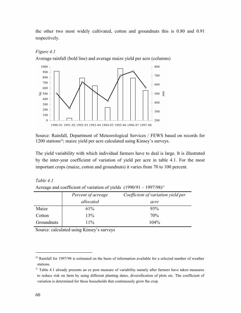
60

the other two most widely cultivated, cotton and groundnuts this is 0.80 and 0.91 respectively. Figure 4.1 Average rainfall (bold line) and average maize yield per acre (columns)

Source: Rainfall, Department of Meteorological Services / FEWS based on records for 1200 stations20; maize yield per acre calculated using Kinsey�s surveys. The yield variability with which individual farmers have to deal is large. It is illustrated by the inter-year coefficient of variation of yield per acre in table 4.1. For the most important crops (maize, cotton and groundnuts) it varies from 70 to 100 percent. Table 4.1 Acreage and coefficient of variation of yields (1990/91 � 1997/98)21 Percent of acreage

allocated Coefficient of variation yield per

acre Maize 61% 93% Cotton 13% 70% Groundnuts 11% 104% Source: calculated using Kinsey�s surveys

20 Rainfall for 1997/98 is estimated on the basis of information available for a selected number of weather stations.

21 Table 4.1 already presents an ex post measure of variability namely after farmers have taken measures to reduce risk on farm by using different planting dates, diversification of plots etc. The coefficient of variation is determined for those households that continuously grow the crop.

0100

200300

400500

600

700800900

1000

1990-91 1991-92 1992-93 1993-94 1994-95 1995-96 1996-97 1997-98

kg

200

300

400

500

600

700

800

mm

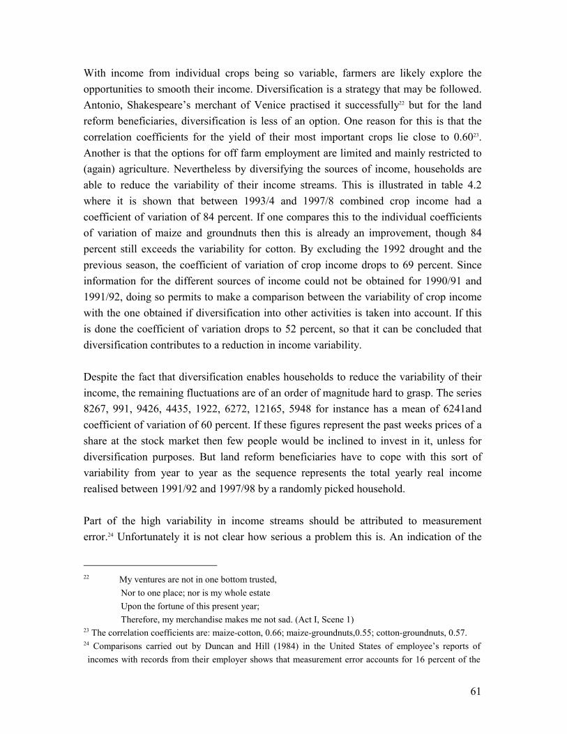
61

With income from individual crops being so variable, farmers are likely explore the opportunities to smooth their income. Diversification is a strategy that may be followed. Antonio, Shakespeare�s merchant of Venice practised it successfully22 but for the land reform beneficiaries, diversification is less of an option. One reason for this is that the correlation coefficients for the yield of their most important crops lie close to 0.6023. Another is that the options for off farm employment are limited and mainly restricted to (again) agriculture. Nevertheless by diversifying the sources of income, households are able to reduce the variability of their income streams. This is illustrated in table 4.2 where it is shown that between 1993/4 and 1997/8 combined crop income had a coefficient of variation of 84 percent. If one compares this to the individual coefficients of variation of maize and groundnuts then this is already an improvement, though 84 percent still exceeds the variability for cotton. By excluding the 1992 drought and the previous season, the coefficient of variation of crop income drops to 69 percent. Since information for the different sources of income could not be obtained for 1990/91 and 1991/92, doing so permits to make a comparison between the variability of crop income with the one obtained if diversification into other activities is taken into account. If this is done the coefficient of variation drops to 52 percent, so that it can be concluded that diversification contributes to a reduction in income variability. Despite the fact that diversification enables households to reduce the variability of their income, the remaining fluctuations are of an order of magnitude hard to grasp. The series 8267, 991, 9426, 4435, 1922, 6272, 12165, 5948 for instance has a mean of 6241and coefficient of variation of 60 percent. If these figures represent the past weeks prices of a share at the stock market then few people would be inclined to invest in it, unless for diversification purposes. But land reform beneficiaries have to cope with this sort of variability from year to year as the sequence represents the total yearly real income realised between 1991/92 and 1997/98 by a randomly picked household. Part of the high variability in income streams should be attributed to measurement error.24 Unfortunately it is not clear how serious a problem this is. An indication of the

22 My ventures are not in one bottom trusted,

Nor to one place; nor is my whole estate Upon the fortune of this present year; Therefore, my merchandise makes me not sad. (Act I, Scene 1)

23 The correlation coefficients are: maize-cotton, 0.66; maize-groundnuts,0.55; cotton-groundnuts, 0.57. 24 Comparisons carried out by Duncan and Hill (1984) in the United States of employee�s reports of incomes with records from their employer shows that measurement error accounts for 16 percent of the

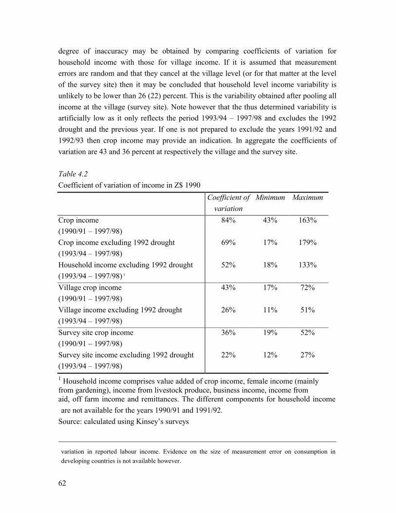
62

degree of inaccuracy may be obtained by comparing coefficients of variation for household income with those for village income. If it is assumed that measurement errors are random and that they cancel at the village level (or for that matter at the level of the survey site) then it may be concluded that household level income variability is unlikely to be lower than 26 (22) percent. This is the variability obtained after pooling all income at the village (survey site). Note however that the thus determined variability is artificially low as it only reflects the period 1993/94 � 1997/98 and excludes the 1992 drought and the previous year. If one is not prepared to exclude the years 1991/92 and 1992/93 then crop income may provide an indication. In aggregate the coefficients of variation are 43 and 36 percent at respectively the village and the survey site. Table 4.2 Coefficient of variation of income in Z$ 1990

Coefficient of variation

Minimum Maximum

Crop income (1990/91 � 1997/98)

84% 43% 163%

Crop income excluding 1992 drought (1993/94 � 1997/98)

69% 17% 179%

Household income excluding 1992 drought (1993/94 � 1997/98) 1

52% 18% 133%

Village crop income (1990/91 � 1997/98)

43% 17% 72%

Village income excluding 1992 drought (1993/94 � 1997/98)

26% 11% 51%

Survey site crop income (1990/91 � 1997/98)

36% 19% 52%

Survey site income excluding 1992 drought (1993/94 � 1997/98)

22% 12% 27%

1 Household income comprises value added of crop income, female income (mainly from gardening), income from livestock produce, business income, income from aid, off farm income and remittances. The different components for household income are not available for the years 1990/91 and 1991/92.

Source: calculated using Kinsey�s surveys

variation in reported labour income. Evidence on the size of measurement error on consumption in developing countries is not available however.

63

The range of estimates for the coefficient of variation of household income variability which varies from 22 to 43 percent and which are determined for the aggregate are only realistic if it is believed that households informally pool all income within the village or at the survey site. But the literature, which tests such pooling generally does not report much evidence in support for it, so that a realistic level of income variability should be exceed the range presented above. On the other hand if household income is measured with error then 52 percent is an upper bound for the coefficient of variation for household income for the period excluding the 1992 drought. If the difference in variability between total and crop income for the period after the drought is extrapolated to the period including it, then 60 percent would be a conservative estimate for the upper bound of the coefficient of variation for total income. The ranges 22-43 and 52-60 then define the borders within which the coefficient of variation for household income should be found. This suggests a very high level of income variability and it is therefore reasonable to expect other coping mechanisms to be important. Financial services could fill the gap, but formal crop insurance is not available to smallholder farmers in Zimbabwe. Formal credit is, but lending is mostly seasonal and related to production. The Cotton Company of Zimbabwe and the Cotton Marketing Board provide inputs on credit. In 1996 45 percent of the farmers that grew cotton made use of this facility. Loans for activities like livestock fattening, breeding and stocking can be obtained from the Agricultural Finance Corporation (AFC), who also gives loans for the production of crops like tobacco. Little to no credit available from these institutions can be used for consumptive purposes so that a household wanting to delink consumption from income using credit has to make use of informal arrangements.25 But informal credit for consumption smoothing purposes is only available to deal with idiosyncratic risks and not with the main source of covariate risk, lack of rain (Kinsey, Burger and Gunning, 1998). This leaves households with a strong incentive to accumulate stocks of liquid assets. Storing food is one possibility. Joseph recommended this to the Pharaoh of Egypt somewhere around 1800 BC, when he prophesied Egypt to enjoy 7 years of prosperity followed by 7 years of famine. The sampled families still follow Joseph�s advice. In bad agricultural seasons like 1992 or 1995 the amounts stored were insufficient to last most 25 An exception are the grain loans made available during the 1995 drought, but whose continuity is under threat.

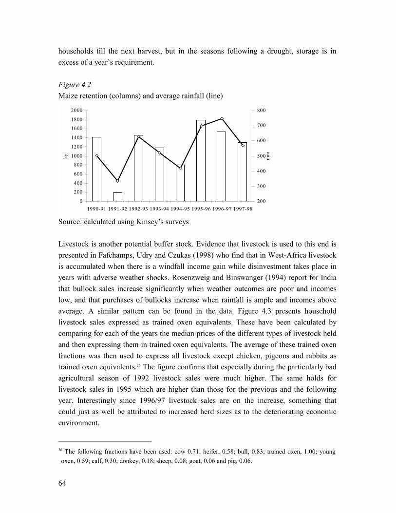
64

households till the next harvest, but in the seasons following a drought, storage is in excess of a year�s requirement. Figure 4.2 Maize retention (columns) and average rainfall (line)

Source: calculated using Kinsey�s surveys Livestock is another potential buffer stock. Evidence that livestock is used to this end is presented in Fafchamps, Udry and Czukas (1998) who find that in West-Africa livestock is accumulated when there is a windfall income gain while disinvestment takes place in years with adverse weather shocks. Rosenzweig and Binswanger (1994) report for India that bullock sales increase significantly when weather outcomes are poor and incomes low, and that purchases of bullocks increase when rainfall is ample and incomes above average. A similar pattern can be found in the data. Figure 4.3 presents household livestock sales expressed as trained oxen equivalents. These have been calculated by comparing for each of the years the median prices of the different types of livestock held and then expressing them in trained oxen equivalents. The average of these trained oxen fractions was then used to express all livestock except chicken, pigeons and rabbits as trained oxen equivalents.26 The figure confirms that especially during the particularly bad agricultural season of 1992 livestock sales were much higher. The same holds for livestock sales in 1995 which are higher than those for the previous and the following year. Interestingly since 1996/97 livestock sales are on the increase, something that could just as well be attributed to increased herd sizes as to the deteriorating economic environment.

26 The following fractions have been used: cow 0.71; heifer, 0.58; bull, 0.83; trained oxen, 1.00; young oxen, 0.59; calf, 0.30; donkey, 0.18; sheep, 0.08; goat, 0.06 and pig, 0.06.

0

200

400

600

800

1000

1200

1400

1600

1800

2000

1990-91 1991-92 1992-93 1993-94 1994-95 1995-96 1996-97 1997-98

kg

200

300

400

500

600

700

800

mm

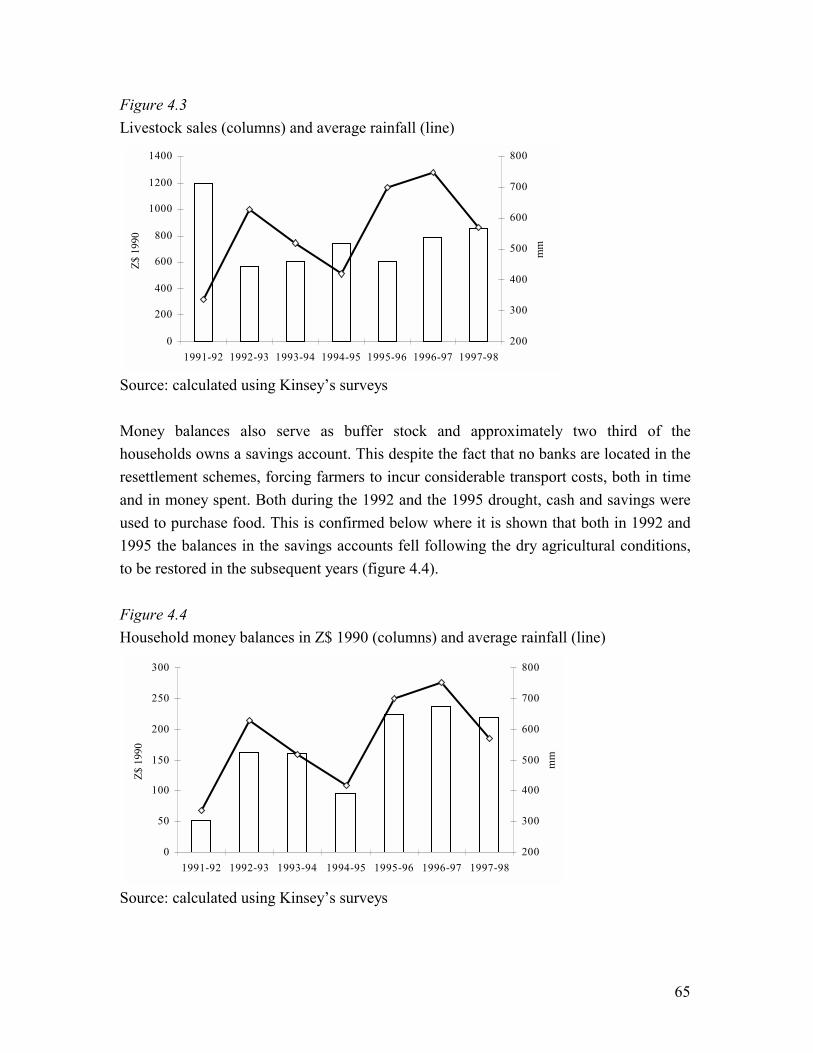
65

Figure 4.3 Livestock sales (columns) and average rainfall (line)

Source: calculated using Kinsey�s surveys Money balances also serve as buffer stock and approximately two third of the households owns a savings account. This despite the fact that no banks are located in the resettlement schemes, forcing farmers to incur considerable transport costs, both in time and in money spent. Both during the 1992 and the 1995 drought, cash and savings were used to purchase food. This is confirmed below where it is shown that both in 1992 and 1995 the balances in the savings accounts fell following the dry agricultural conditions, to be restored in the subsequent years (figure 4.4). Figure 4.4 Household money balances in Z$ 1990 (columns) and average rainfall (line)

Source: calculated using Kinsey�s surveys

0

200

400

600

800

1000

1200

1400

1991-92 1992-93 1993-94 1994-95 1995-96 1996-97 1997-98

Z$ 1

990

200

300

400

500

600

700

800

mm

0

50

100

150

200

250

300

1991-92 1992-93 1993-94 1994-95 1995-96 1996-97 1997-98

Z$ 1

990

200

300

400

500

600

700

800

mm

66

Using the same data Kinsey, Gunning and Burger (1998) found that livestock sales and cash balances provided most cash to deal with the consequences of the 1992 and 1995 droughts (their results are presented in the next chapter, table 5.1). But it is reasonable to expect that these buffer stocks are also put to use during less extreme events. A way to investigate whether this is done successfully is to consider the variability of consumption. If it is found to be low then it can be concluded that a buffer stock strategy works well. The coefficient of variation is not low however. In fact it is very high: 49 percent on average (with a maximum of 200 percent). This degree of consumption variability seems unrealistically high if only because the formula presented in section 4.5 suggests that to avoid such variability in consumption households would be prepared to forego 25 percent of their average consumption. This is such a large fraction of total household consumption that it can hardly be reconciled with the absence of financial services. But like income, part of the variability in consumption might be due to measurement error. To get an indication of the minimum degree of variability consider the coefficients of variation of consumption at the village (survey site) level: on average these are 25 and 16 percent respectively, with corresponding maximums of 53 and 21 percent. 25 and 16 percent provide a lower bound on the consumption variability as they reflect the aggregate variation in consumption. If one would be prepared to accept a sizeable degree of mismeasurement at the household level of, say, 30 to 50 percent then one would still be left with a coefficient of variation of 25 to 35 percent. To avoid such a degree of consumption variability a household with a relative degree of risk aversion would be prepared to forego 6 to 12 percent of average household consumption. This is a high fraction and it would seem that this would constitute a large demand for financial services.

4.3 Deriving a Consumption Rule In the previous section expenditure variability was established to be high and it was suggested that part of this variation is due to inaccuracies in consumption measurement. It has also been established that farmers face highly fluctuating income, that formal financial markets are absent and that households rely on buffer stocks to insulate consumption from income shocks. To verify whether the consumption variability reported in the previous section is realistic an attempt is made in this and the next section, to numerically derive the

67

optimal degree of consumption variability for an impatient household (i.e. its rate of time preference exceeds the rate of return on the buffer stock) that relies on a buffer stock strategy using a safe buffer stock in the face of a variable, exogenous, income stream. And as income variability could also not be established accurately either, consumption rules are derived under three scenarios with respectively low, medium and high income variability. The approach followed is based on Deaton (1989, 1991) and Obstfeld and Rogoff (1996). The household�s decision problem is to determine the optimal amount of consumption in the face of an uncertain future. If the farmer would know that next year was going to be a drought year, he would decide to save more (and consume less) today in order to avoid the worst suffering during the drought year. And if he would be aware that next season was going to be a good one, then he would reduce the size of his buffer stock (and increase consumption in the current period) to immediately benefit from the fruits of a good season to come. The problem is of course that it is not known what the future will bring. The households decision problem can therefore be described as deciding on the optimal level of current consumption (i.e. the amount of current consumption that maximises lifetime utility) given the available resources (income and assets carried over from the previous period), knowing the distribution of future income realisations but being unaware of its actual realisations. It is assumed that income is exogenously determined. Obviously this is a simplification, but one that may hold in an environment with rain-fed farming, where rainfall has a determining influence on the crop realisations. That households know the distribution of their income process (or, for that matter of the rainfall pattern) is another strong condition. It can be defended on the grounds that in many rural areas crop yields are stationary and their variances well understood by farmers. Furthermore it is assumed that assets yield a constant rate of return, r, when they are transferred from one period to the next. The return can be negative or positive. It is likely to be negative if assets are kept in the form of food stores and affected by storage losses or as cash balances that reduce in value over time due to inflation. A positive rate of return can be expected for livestock whose value increases through breeding and weight increase. The evolution of assets, at, over time, t, is given in (4.1) as a function of income, yt,, and consumption ct:

tttt cyara −++= −1)1( . (4.1)

68

Though it is intended to arrive at a consumption rule for a situation without financial markets, assume for now that financial markets exist and that households can borrow as much as they wish at rates identical to the lending rate. In that case asset possessions can be positive or negative in which case they represent borrowings. Despite the presence of financial markets the possibility of Ponzi schemes, in which the household has access to infinite resources by borrowing money and repaying the interest and the principal by borrowing even more money has to be ruled out. This is expressed in condition (4.2) that states that the net present value of a household�s asset holdings is not allowed to be negative:

0)1(lim 1 ≥+ ++−

∞→ TtT

T ar (4.2)

must hold. Households are assumed to live infinitely. Obviously this is a simplification but one that can be justified on the ground that households, or families, in developing countries are usually quite long lived. The household�s optimisation problem is to maximise the discounted (ρ is the rate of time preference) expected value of lifetime utility, Ut (E is the mathematical conditional expectations operator):

)(0

ττ

τρ +

∞

=

+�= t

tt cuEU (4.3)

subject to the constraints (4.1 and 4.2). The utility function is twice differentiable and strictly concave: u�(ct) > 0 and u��(ct) < 0. Imposing a concave utility function automatically implies that households have an incentive to smooth consumption. This follows from the fact that a given increase in consumption above a certain value provides the household with less extra utility than the loss in utility the household would experience if it had to deal with a similar reduction of consumption below this value. The household does not know what it will earn in the future. So it can only optimise its consumption given the resources it has available today. Let xt denote the resources available for consumption (also called cash on hand). It is defined as:

69

ttt yarx ++= −1)1( (4.4)

A condition that should hold if a current consumption plan is to be optimal, is that future utility, Ut+1, is maximised as well, subject to the wealth constraint that holds at that time (xt+1). But the future wealth constraint depends on the current level of consumption. After all it follows from (4.1) and (4.4) that

11 )()1( ++ +−+= tttt ycxrx . (4.5)

Applying Bellman�s reasoning, which suggests the choice of the optimal level of ct is the one that maximises Ut = u(ct) + ρ V (xt+1) subject to (4.5), where Vt (xt+1) is a value function that represents the constrained maximal value of Ut+1 the household�s maximisation problem (in other words, a household that plans to optimise starting tomorrow can do no better today than to optimise taking future optimal plans as given) can now be written as:

)()(max)( 11 +++= ttttctt xVEcuxVt

ρ (4.6)

subject to (4.5). As the value function depends on resources the information available at date t it has a subscript t. Taking the first order condition of (4.6) gives:

0)()1()( 1'

1' =+− ++ tttt xVErcu ρ . (4.7)

Equation (4.7) is still not usable as basis for a consumption rule. But realise that for an optimising household it does not matter whether it puts its marginal unit of wealth to savings or to consumption. After all an initial allocation in which the marginal value of savings exceeds that of consumption cannot be optimal as the household raise its lifetime utility by reducing consumption a bit. The implication is that for every date under a maximising consumption plan (see annex 4.1 for a derivation):

)()( ''tttt cuxV = (4.8)

holds. Substituting (4.8) into (4.7) yields the stochastic Euler equation:

70

( ))(')1()(' 1++= ttt cuErcu ρ (4.9)

This equation is central to the modern view on consumption, namely that households attempt to keep the marginal utility of consumption constant over time. It states that, in discounted utility terms rational forward looking households will not want marginal consumption to be worth more in one period than another (adjusted for a time factor) and shows that in the optimum the family is indifferent between consuming her last dollar in the current period, or saving it and consuming it next period. In the presence of complete financial markets, the household would be able to optimally smooth its consumption and have complete certainty about the level of consumption at all dates. If the household faces a bad income draw and is out of assets, it borrows money to repay later. If the available resources (income plus accumulated assets) exceed the requirements for optimal consumption, it puts money in the bank to prepare for less fortunate circumstances. So despite the fact that the household does not know what the future will bring, in the presence of complete financial markets it is able to obtain a constant level of consumption. Now let�s make the model more realistic and let formal and informal financial markets be absent. A trivial but important consequence of this is that households can no longer have negative asset holdings. Hence to equation (4.1) a borrowing constraint has to be added stating that household assets always have to be larger or equal to zero: 0≥ta .

The asset constraint ensures that consumption can, at maximum, be current income plus the value of the stock of assets. Now the household can be confronted with two situations: (i) in which the asset constraint makes itself felt. The household has consumed all its income and assets and would like to borrow but cannot. With all assets consumed, the marginal utility of an extra unit of current consumption is higher than the expected marginal utility to be derived from saving this unit. (ii) in which the asset constraint does not limit household decisions and where current income plus assets are sufficient for the stochastic Euler equation to hold. The marginal utility of current consumption is equated to expected future marginal utility and the household would not wish to borrow money even if it were able to do so.

71

These two cases can be brought together in a single expression, in which the second part is the stochastic Euler equation presented as equation (4.9):

[ ]{ })(')1();('max)(' 1++Ε= tttt curxucu ρ (4.10)

Due to the presence of borrowing constraints a smooth profile of future consumption is no longer assured. In some years when the household is out of assets and income is low, the family faces a situation in which there is little to consume namely the low income only. In other periods at which income is sufficiently high, the household will be able to consume more. In those years it consumes its desired level and accumulates buffer stocks to be used in periods in which income is low. It follows that in the absence of financial markets consumption becomes variable. But, due to the accumulated savings its variability is less than that for income. To obtain an expression for consumption, expression (4.10) is inverted. This is allowed because u�(ct) is a monotonically decreasing function. Inversion gives:

[ ]{ })(')1(';min 11

+− +Ε= tttt curuxc ρ (4.11)

Expression (4.11) shows that the current level of resources (xt) solely determines consumption. This allows writing the consumption function in a very general form as: )( tt xcc = . Here is stated that consumption is stochastic (xt is a random variable) and

depends on the availability of resources. Substituting the expression for consumption for the current and the next period into the previous expression, yields:

[ ]{ })(')1(';min)( 11

+− +Ε= tttt xcuruxxc ρ . (4.12)

Finally replace 1+ta by the sequence from which it originates:

11 ))()(1( ++ +−+= tttt yxcxrx to obtain equation (4.13):

[ ]{ })}()(1({')1(';min)( 1

1tttttt xcxrycuruxxc −+++Ε= +

− ρ . (4.13)

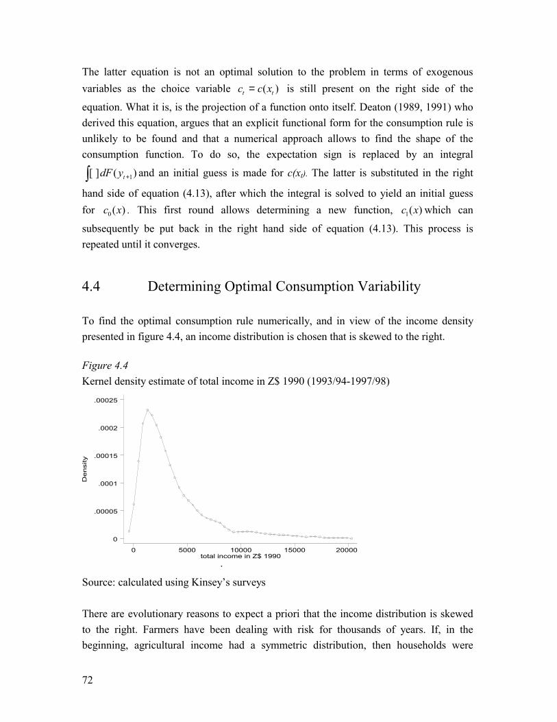
72

The latter equation is not an optimal solution to the problem in terms of exogenous variables as the choice variable )( tt xcc = is still present on the right side of the

equation. What it is, is the projection of a function onto itself. Deaton (1989, 1991) who derived this equation, argues that an explicit functional form for the consumption rule is unlikely to be found and that a numerical approach allows to find the shape of the consumption function. To do so, the expectation sign is replaced by an integral

)(][ 1+� tydF and an initial guess is made for c(xt). The latter is substituted in the right

hand side of equation (4.13), after which the integral is solved to yield an initial guess for )(0 xc . This first round allows determining a new function, )(1 xc which can

subsequently be put back in the right hand side of equation (4.13). This process is repeated until it converges.

4.4 Determining Optimal Consumption Variability To find the optimal consumption rule numerically, and in view of the income density presented in figure 4.4, an income distribution is chosen that is skewed to the right. Figure 4.4 Kernel density estimate of total income in Z$ 1990 (1993/94-1997/98)

Densi

ty

.total income in Z$ 1990

0 5000 10000 15000 20000

0

.00005

.0001

.00015

.0002

.00025

Source: calculated using Kinsey�s surveys There are evolutionary reasons to expect a priori that the income distribution is skewed to the right. Farmers have been dealing with risk for thousands of years. If, in the beginning, agricultural income had a symmetric distribution, then households were

73

facing an equal probability of low and high outcomes. Given the shape of their utility function in which the utility loss from outcomes below a given point is larger than the benefit associated with an outcome above that point, farmers would have had a strong incentive to alter the shape of their income distribution to a form where low incomes are less probable. Through the selection of plants and development of cultivation methods they might have been able to do so with a distribution that is skewed to the right as the result. And as crop income is skewed to the right, so is non agricultural wage income (which cannot be negative) and so are profits from entrepreneurial activities (because negative profits cannot be sustained for a prolonged period), so that the total income distribution is also skewed to the right. It is assumed in the simulations that the income process follows a lognormal distribution with mean 100. To do justice to the empirical findings for income variation and the dispersion therein, three cases are considered: one in which income has a coefficient of variation of 30, one where it is 50 and one where the coefficient of variation is 80.27 30 represents a situation with complete income pooling within the village, 50 a situation where this is largely absent and 80 is the upper bound of potential income variability. By choosing an income process with a constant mean it is suggested that the income process is stationary. This appears to contradict Gunning et al. (2000) who, after comparing household incomes between 1983/84 and 1995, conclude that the incomes of land reform beneficiaries increased substantially. But for the period 1995-1999 this income growth appears to have disappeared. At least this can be concluded from regressing real household income on a time dummy and a rainfall variable. The time coefficient is insignificant (t-stat of 0.45) while that for rainfall is significant (t-stat of 5.41). Apart from a different income distribution, the simulation model uses the same utility function and parameters as Deaton (1989) did. The utility function is the iso-elastic one:

)1(1)(

)1(1

σ

σ

−=

−ccu ,

where σ is the intertemporal elasticity of substitution. Presented is the consumption function for σ =1/2, implying a degree of relative risk aversion of 2. Having taken a lognormal distribution, negative income draws are of no concern, so that the distribution

27 This is an approximation of the income distributions presented in figure 4. A Shapiro-Wilks test rejects the hypothesis that income follows a lognormal distribution.

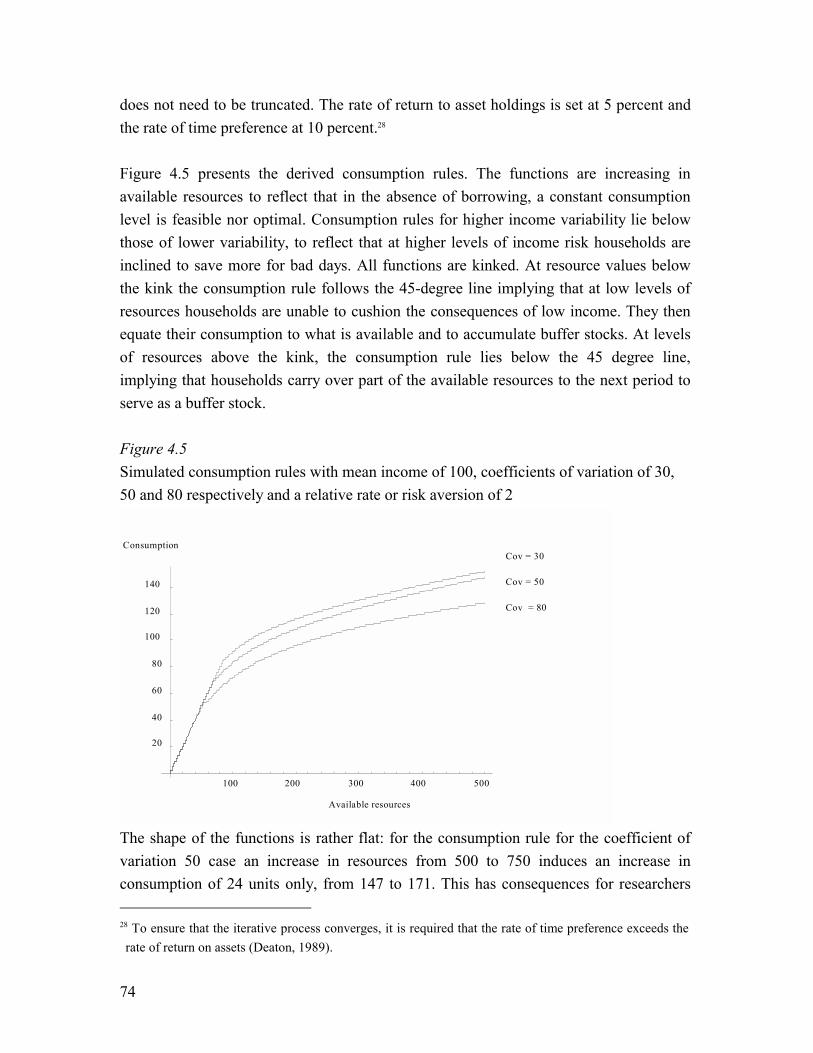
74

does not need to be truncated. The rate of return to asset holdings is set at 5 percent and the rate of time preference at 10 percent.28 Figure 4.5 presents the derived consumption rules. The functions are increasing in available resources to reflect that in the absence of borrowing, a constant consumption level is feasible nor optimal. Consumption rules for higher income variability lie below those of lower variability, to reflect that at higher levels of income risk households are inclined to save more for bad days. All functions are kinked. At resource values below the kink the consumption rule follows the 45-degree line implying that at low levels of resources households are unable to cushion the consequences of low income. They then equate their consumption to what is available and to accumulate buffer stocks. At levels of resources above the kink, the consumption rule lies below the 45 degree line, implying that households carry over part of the available resources to the next period to serve as a buffer stock. Figure 4.5 Simulated consumption rules with mean income of 100, coefficients of variation of 30, 50 and 80 respectively and a relative rate or risk aversion of 2

100 200 300 400 500

20

40

60

80

100

120

140

Consumption

Available resources

Cov = 30

Cov = 50

Cov = 80

The shape of the functions is rather flat: for the consumption rule for the coefficient of variation 50 case an increase in resources from 500 to 750 induces an increase in consumption of 24 units only, from 147 to 171. This has consequences for researchers 28 To ensure that the iterative process converges, it is required that the rate of time preference exceeds the rate of return on assets (Deaton, 1989).

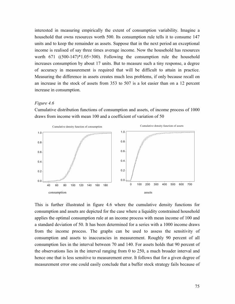
75

interested in measuring empirically the extent of consumption variability. Imagine a household that owns resources worth 500. Its consumption rule tells it to consume 147 units and to keep the remainder as assets. Suppose that in the next period an exceptional income is realised of say three times average income. Now the household has resources worth 671 ((500-147)*1.05+300). Following the consumption rule the household increases consumption by about 17 units. But to measure such a tiny response, a degree of accuracy in measurement is required that will be difficult to attain in practice. Measuring the difference in assets creates much less problems, if only because recall on an increase in the stock of assets from 353 to 507 is a lot easier than on a 12 percent increase in consumption. Figure 4.6 Cumulative distribution functions of consumption and assets, of income process of 1000 draws from income with mean 100 and a coefficient of variation of 50

consumption assets This is further illustrated in figure 4.6 where the cumulative density functions for consumption and assets are depicted for the case where a liquidity constrained household applies the optimal consumption rule at an income process with mean income of 100 and a standard deviation of 50. It has been determined for a series with a 1000 income draws from the income process. The graphs can be used to assess the sensitivity of consumption and assets to inaccuracies in measurement. Roughly 90 percent of all consumption lies in the interval between 70 and 140. For assets holds that 90 percent of the observations lies in the interval ranging from 0 to 250, a much broader interval and hence one that is less sensitive to measurement error. It follows that for a given degree of measurement error one could easily conclude that a buffer stock strategy fails because of

0.0

0.2

0.4

0.6

0.8

1.0

40 60 80 100 120 140 160 180

Cumulative density function of consumption

0.0

0.2

0.4

0.6

0.8

1.0

0 100 200 300 400 500 600 700

Cumulative density function of assets

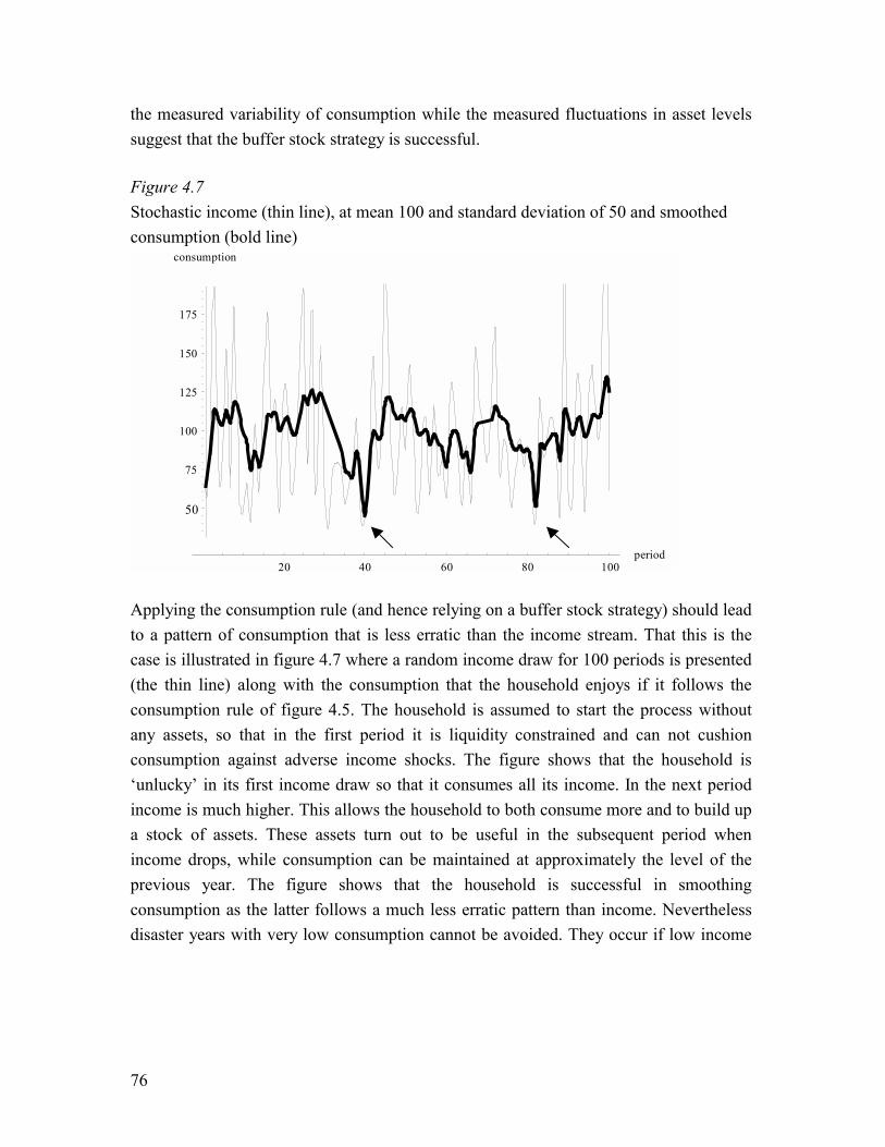
76

the measured variability of consumption while the measured fluctuations in asset levels suggest that the buffer stock strategy is successful. Figure 4.7 Stochastic income (thin line), at mean 100 and standard deviation of 50 and smoothed consumption (bold line)

20 40 60 80 100period

50

75

100

125

150

175

consumption

Applying the consumption rule (and hence relying on a buffer stock strategy) should lead to a pattern of consumption that is less erratic than the income stream. That this is the case is illustrated in figure 4.7 where a random income draw for 100 periods is presented (the thin line) along with the consumption that the household enjoys if it follows the consumption rule of figure 4.5. The household is assumed to start the process without any assets, so that in the first period it is liquidity constrained and can not cushion consumption against adverse income shocks. The figure shows that the household is �unlucky� in its first income draw so that it consumes all its income. In the next period income is much higher. This allows the household to both consume more and to build up a stock of assets. These assets turn out to be useful in the subsequent period when income drops, while consumption can be maintained at approximately the level of the previous year. The figure shows that the household is successful in smoothing consumption as the latter follows a much less erratic pattern than income. Nevertheless disaster years with very low consumption cannot be avoided. They occur if low income

77

coincides after a sequence of low income draws when the households is out of buffer stocks. In the figure there are two of such years, which are indicated by arrows.29 By repeating the process of randomly drawing an income series and determining the optimal consumption the coefficient of variation of consumption after applying a buffer stock strategy can be determined. This is done in a Monte Carlo simulation, in which a 1000 times the mean and variance of income, consumption and buffer stocks are established for a sequence of 100 periods. The mean values for these variables are presented in table 4.3. The table illustrates that the average stock of assets, responds strongly to the variability of the income process. In the coefficient of variation (cov) 80 case, average asset holdings are more than two and a half time as large than those in the cov 50 situation and nearly six times as large as in the cov 30 case. In all cases does average consumption slightly exceed mean income, which follows from the fact that households earn a positive return on asset holdings. The accumulation of assets allows the household to reduce consumption variability to a large extent. Compared to a situation where no buffer stock strategy is followed, the coefficient of variation drops from 30 to 17, from 50 to 17 and from 80 to 21 respectively. The simulated results can be used to validate the coefficient of variation for consumption found in the data. The simulations suggest that after applying a buffer stock strategy with a safe asset the remaining coefficient of variation for consumption is approximately 13 to 20 percent, where 13 might be considered a conservative estimate for the coefficient of variation of household consumption and 18-20 more realistic. These measures are lower than those obtained from the data where the degree of consumption variability was put to lie between 25 and 35 percent. This is what is to be expected given the assumption of an ideal buffer stock in the simulations.

29 The finding that disaster conditions only occur after a sequence of bad shocks suggests that with careful monitoring indications that such a condition is about to occur can be obtained well in advance.

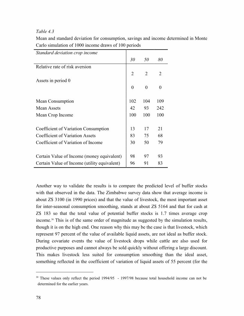
78

Table 4.3 Mean and standard deviation for consumption, savings and income determined in Monte Carlo simulation of 1000 income draws of 100 periods Standard deviation crop income

30

50

80 Relative rate of risk aversion

2 2

2

Assets in period 0 0

0

0

Mean Consumption 102 104 109 Mean Assets 42 93 242 Mean Crop Income 100 100 100 Coefficient of Variation Consumption 13 17 21 Coefficient of Variation Assets 83 75 68 Coefficient of Variation of Income 30 50 79 Certain Value of Income (money equivalent) 98 97 93 Certain Value of Income (utility equivalent) 96 91 83

Another way to validate the results is to compare the predicted level of buffer stocks with that observed in the data. The Zimbabwe survey data show that average income is about Z$ 3100 (in 1990 prices) and that the value of livestock, the most important asset for inter-seasonal consumption smoothing, stands at about Z$ 5164 and that for cash at Z$ 183 so that the total value of potential buffer stocks is 1.7 times average crop income.30 This is of the same order of magnitude as suggested by the simulation results, though it is on the high end. One reason why this may be the case is that livestock, which represent 97 percent of the value of available liquid assets, are not ideal as buffer stock. During covariate events the value of livestock drops while cattle are also used for productive purposes and cannot always be sold quickly without offering a large discount. This makes livestock less suited for consumption smoothing than the ideal asset, something reflected in the coefficient of variation of liquid assets of 55 percent (for the

30 These values only reflect the period 1994/95 - 1997/98 because total household income can not be determined for the earlier years.

79

period including the 1992 drought) and 47 percent for the period that excludes this disaster year.31 Compare this to that for the safe asset (table 4.3) of 75 percent. It confirms that ideal assets are more suited for consumption smoothing purposes than those available in practice and that the coefficient of variation of consumption obtained in the simulations is a lower bound. The estimate of a coefficient of variation of 25 to 35 percent for consumption is therefore considered realistic.

4.5 Benefits from Introducing Formal Financial Institutions Despite the accumulation and depletion of buffer stocks, in the absence of formal financial institutions households do not eliminate all variation in consumption. The consequences of the remaining variability may be grave as is illustrated by the fact that figure 4.7 comprises at least 2 years which would qualify as disaster years, and a few more that are particularly bad. Even in the presence of an ideal buffer stock, households are still to gain from financial services that allow them to further stabilise their consumption. A complete income insurance scheme would eliminate all consumption variability by guaranteeing the farmer his average income each year by collecting premium in years when income exceeds average and paying indemnities in all other years. But how much will farmers gain from such a service? The price farmers are prepared to pay for complete insurance can be determined by calculating the risk premium they would be prepared to pay to attain a certain income. This risk premium can be approximated by the formula:

2

21

)(υπ R

cE t

≈

where π indicates the risk premium, R the relative rate of risk aversion (2 in our case) and υ the coefficient of variation of consumption (Newbery and Stiglitz, 1981). Application of this formula shows that uninsured and without the use of buffer stocks, the risk premium would lie between 9 percent and 64 percent of average income (depending on whether the coefficient of variation of income is 30, 50 or 80).32 Through

31 One could argue that households adapt their size in response to crises and that for that reason per capita measures are more appropriate. To investigate this, the presented coefficients were also been determined per adult equivalent They only differed marginally from the coefficients presented here..

32 These estimates are halved for households with a relative degree of risk aversion of 1.

80

self-insurance, and in the presence of safe assets, farmers may reduce the variability of consumption to a considerable extent but still they would be prepared to pay about 2 to 4 percent (depending on whether the coefficient of variation is 13, 17 or 21) of their average consumption as risk premium. If one relies on the coefficient of variation from the data this would lay between 6 to 12 percent. These figures are lower bounds because they are obtained for a situation where households also accumulate buffer stocks. Formal financial institutions may also offer a service which is not complementary to the self-insurance strategy of farmers but which substitutes it. Such would be attractive if the cost of formal insurance is lower than the opportunity costs of self-insurance. The opportunity costs of self-insurance are embedded in the fact that households have to accumulate assets despite the fact that the rate of time preference exceeds the rate of return on those assets. Households are nevertheless prepared to bear this opportunity cost, because of the benefit received from the reduction in consumption variability. To determine the money metric value of the opportunity costs of accumulating assets let y i

pv be the certain value of income which allows the household to achieve the same discounted expected utility as the consumption stream that follows from the optimal consumption rule with ideal buffer stocks:

)()1(

1)()1(

1,

0,

0ti

N

tt

pvti

N

tt cEvyv ��

== +=

+ δδ. (4.14)

The right hand site of equation (4.14) is known from the Monte Carlo simulations so that y i

pv , fixed for all t, can be determined. The certainty equivalent income values are presented in table 4.2. They are 96, 91 and 83 for the standard deviation 30, 50 and 80 cases respectively implying that farmers would be prepared to forego 4 to 17 percent of their average income to obtain a stable income and to forego the necessity of accumulating buffer stocks. If one wants to be more conservative and assume a relative rate or risk aversion of 1 then the range would lie between 2 and 10 percent. These figures are presented in annex 4.2.33

33 This estimate does not include the benefits from specialisation that the introduction of financial services also make possible.

81

4.6 Discussion In this chapter the question has been posed why financial instruments that allow rural households to smooth their consumption in the face of variable income are not offered. In search of an answer it has been explored whether the demand for financial services is low. This could be the case because households are able to successfully smooth their income through diversification. This turns out not to be case. In section 4.2 income is found to vary a lot. The other possibility is that households are able to shield their consumption from income fluctuations through a buffer stock strategy. The variability in the expenditure information shows that this is not the case either. This suggests that rural households should have a large, unmet demand for consumption smoothing services. Part of the observed consumption variability, has to be attributed to inaccuracies in measurement. Since the degree of inaccuracy is unknown another approach to derive income variability is attempted. In this approach a consumption rule for a risk averse household that relies on a buffer stock strategy and a safe buffer stock is derived numerically after which in a Monte Carlo simulation the variability of consumption is established. The size of the premium households (are prepared to) pay according to the simulation reconciles only partly the contradictory findings mentioned in the introduction. From the careful scenario it may be concluded that the welfare gains of the introduction of financial markets are at least 4 percent. This might not be induce the provision if financial services. But households are heterogeneous and for some the demand may be much higher especially as the percentage rises quickly, depending on the scenario. It may even be as high as 17 percent. The variability of the consumption data suggests percentages varying between 6 and 12 percent. These values should be halved for households with a lower degree of risk aversion. It should be noted here that these values are based on averages. For individual households that experience higher (lower) variability of consumption, the amounts they would be prepared are higher (lower). Based on these estimates it is felt that there exists a substantial unmet demand for consumption smoothing financial services. So if there is a demand for financial services of a magnitude that monitoring costs to deal with asymmetric information can be covered then the question arises why these services have not been introduced yet. Several reasons may be advanced. High fixed costs and a financial sector reluctant to provide the required money is one. In the presence of sunk costs not all goods that can conceivably be produced are taken into production. Especially goods with high sunk costs will not be fabricated (Krugman, 1980; Romer,

82

1994). Covariate risk is another. A local insurance company could easily go bankrupt if it is confronted with the consequences of an all-encompassing drought like the one in 1992. This can be overcome through a further integration in world markets, but as yet the Zimbabwean insurance industry does not have access to the global reinsurance market. This despite the fact that the risks that potentially are on offer, such as drought risk, may be attractive (for diversification purposes) for international insurers. Another possibility may be sought in the institutional environment. To be prepared to actually buy insurance, farmers have to be assured that they will receive indemnity payments when they are entitled to obtain them. But in an environment where much of the risk is covariate and where institutional control is limited, farmers may have little confidence in insurance institutions.34 This in turn leads to absence of an effective demand for insurance coverage despite the fact that farmers would be prepared to pay for a reliable service.

34 Lack of trust was one of the main concerns raised during informal discussions with farmers on whether they would be interested in insurance coverage.

83

Annex 4.1 To arrive at:

)()( ''ttt cuxV = (4.8)

take the first order condition of (4.7) and write it as:

)()1()( 1'

1'

+++= tttt xVErcu ρ . (4.7)

Next replace xt+1 using (4.5) to obtain:

}))(1{()1()( 1'

1'

++ +−++= tttttt ycxrVErcu ρ . (4.7*)

This shows that ct can be expressed as an implicit function of xt:: ct=ct(xt). Substituting this into the Bellman equation gives:

}))()(1{())(()( 11 ++ +−++= tttttttttt yxcxrVExcuxV ρ

Differentiating this with respect to xt gives:

)](1}[))(1{()1()())(()( '1

''''1 tttttttttttt xcycxrVErxcxcuxV

t−+−+++= ++

ρ .

This reduces, after substituting in (4.7) to

)))(1(()1()( 1''

1 ++−++=+ tttttt ycxrVErxV

tρ .

Substituting (4.7) in another time yields the desired expression:

)()( ''ttt cuxV = (4.8)

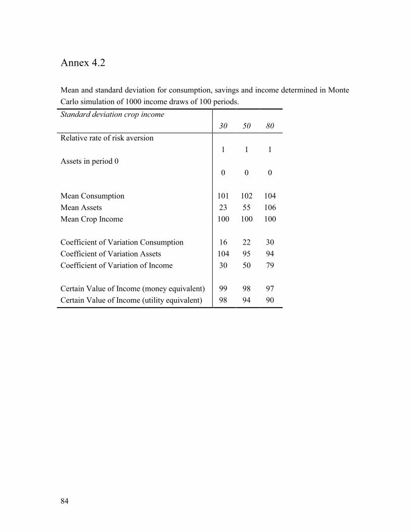
84

Annex 4.2 Mean and standard deviation for consumption, savings and income determined in Monte Carlo simulation of 1000 income draws of 100 periods. Standard deviation crop income

30

50

80 Relative rate of risk aversion

1 1

1

Assets in period 0 0

0

0

Mean Consumption 101 102 104 Mean Assets 23 55 106 Mean Crop Income 100 100 100 Coefficient of Variation Consumption 16 22 30 Coefficient of Variation Assets 104 95 94 Coefficient of Variation of Income 30 50 79 Certain Value of Income (money equivalent) 99 98 97 Certain Value of Income (utility equivalent) 98 94 90

Evidence on Informal Insurance

in the Community

5.1 Introduction

In the previous chapter the high income variability Zimbabwean rural households face has been brought to the fore, along with their attempts to ensure that consumption is not affected by this variability. One way to do so is through the accumulation of buffer stocks. Another is to rely on insurance arrangements. Formal arrangements are absent in Zimbabwe�s rural areas but this does not mean that risks cannot be pooled at all. In fact, rural households are likely to have certain advantages in pooling risks themselves, especially if households know each other well (this reduces the scope for information problems) or if they have extra-legal means of contract enforcement. The possibility to pool risk at the community level is illustrated by the coefficient of variation for crop income (table 4.2). It is 84 percent at the household level, but at the community level the coefficient of variation is much lower. For villages as a whole it is 43 percent and at the survey site, 36 percent implying that there are indeed idiosyncratic

86

shocks that can well be pooled at the community level. Pooling incomes at the village or survey site level would thus help to reduce income risk. In conversations with farmers it materialised that this is not only a theoretical possibility but that it is actively explored. Reciprocal exchanges are common (this even continued during the drought of 1992) and many villagers participate in informal funeral arrangements and work parties or joined savings clubs (women especially).35 A way to explore the existence of mutual insurance at the community level without having to go into detail on each of the existing informal arrangements is to consider whether the consumption of those living in the same community moves in the same direction. After all, even if all incomes are pooled and each household receives its predetermined share from the pool, then at times when aggregate resources are in abundance every household will have more to consume than at times when community resources are scarce. Comovement in consumption between group members is therefore in accordance with full insurance. Comovement in consumption is a condition that will be met in the presence of full insurance, but evidence in support of it does not invalidate other explanations for the same phenomenon. From a permanent income model without insurance or from the consumption rule derived in chapter four, a similar prediction can be derived if the community is confronted with a technology shock.36 Productivity increasing technological shocks probably did not take place in the survey areas since 1992. But to discard this possibility beforehand would be premature, if only because of the structural changes that occurred in the Zimbabwean economy since 1992 (liberalisation; high inflation and more recently a breakdown of the institutional infrastructure). In any case, the reverse does hold: if no, or partial comovement in consumption between villagers is found, then complete insurance through informal arrangements does not exist. Evidence in support of full insurance, has implications for, for instance, the implementation of disaster relief efforts. In the presence of full insurance, targeting is of little importance because the transfer of resources to any member in a community with full insurance will be followed by a redistribution of this addition to aggregate resources amongst the members in the insurance pool. Another implication of full insurance is that

35 Saving clubs are not necessarily informal insurance arrangements, but many are organised in such a way that they allow their members to pool certain risks.

36 In the case of the consumption rule of chapter four, even a good rainfall year could generate such a result.

87

in its presence, poverty will be permanent and escape from it will depend on the availability of sufficient resources in the aggregate. A rejection of the full insurance model implies that the distribution of household endowments is of importance for household consumption, implying for instance a means test to ensure that relief aid reaches the persons in need. To find evidence in support of full insurance would be remarkable. In its presence incentives for shirking are be large (the effort of any participant in the pool has only a marginal impact on his share of income) and participants have less of an incentive to avoid risks. Without accompanying measures both consequences will undermine the functioning of a complete insurance mechanisms. Additionally, households have an incentive to join the insurance ex ante, but those with fortunate income draws will want to renege on their promise to share when they have to make transfers to the unfortunate members in the pool. For these reasons complete consumption insurance may be neither desirable nor possible. Nonetheless Townsend (1994) reports evidence in support of full insurance for households in the Indian ICRISAT villages. But as Ravallion and Chaudhuri (1997) have pointed out, Townsend�s empirical analysis is biased toward the acceptance of the full insurance model. In a careful re-examination of his results, Ravallion and Chaudhuri only found indications for partial insurance. This is a result more commonly found. Cochrane (1991), Mace (1991), Grimard (1997), Deaton (1997) and Ravallion and Jalan (1999) report a certain degree of comovement in consumption across households, but not complete insurance. The test of full insurance is based on the proposition that with perfect risk sharing, consumption at the household level is shielded from idiosyncratic risks and depends solely on the realisation of aggregate risk. Consumption should be independent of the realisation of household income and this is what is tested. The approach is reasonable if buffer stocks are absent. But consider a situation in which this is not the case. Suppose for instance that in a rural setting two subsequent harvests fail completely. Each household�s income is zero but families do not starve as they rely on buffer stocks. In this case a test that considers whether household consumption is independent of household income would find this to be true. But to consider this a situation of full insurance would not be correct. It is not clear for instance whether idiosyncratic shocks are shared in years with positive income. And to label as full insurance a situation in which each household finances its consumption from the sale of its assets, is inappropriate. The illustration is extreme but comparable problems will arise in each instance where buffer stocks are used to deal with shocks. It implies, and this will be

88

derived in the next section, that the common test of full insurance is affected by an omitted variable problem. To deal with this issue a test is developed that takes explicitly into account the accumulation of buffer stocks. Once the test is derived it is empirically tested. Additionally, whether differences in the degree of insurance exist between those living in land reform villages and those living in communal area villages is explored as well. On the one hand, monitoring between land reform beneficiaries is easier because, unlike communal households, they live clustered in villages. On the other hand, resettled households started off as strangers. Though it seems plausible that any distrust that might have existed at the initial phase of land reform will have disappeared after almost 20 years, it cannot be excluded that the fact that households come from different regions (and have different ethic backgrounds) still gives rise to social tensions. Both effects work in opposite directions so that a prior cannot be formulated. Nevertheless, whether differences in informal insurance exist between both groups of households is an interesting issue in itself. Another factor of interest is whether insurance experienced by the poor differs from that of the better off. As was pointed out in chapter two, wealthy households have an incentive to renege on their contribution to the insurance pool. Households that are fortunate in their income outcomes may collude against families experiencing negative income shocks and exclude them from the insurance in an attempt to limit the size of the transfers they have to make. On the other hand marginal utility declines steeply if consumption lies close to the survival threshold. The poor therefore have a greater interest in the proper functioning of insurance arrangements and may for that reason participate more actively in them. In either case, there is reason to believe that differences in the degree of insurance exist between poor and non-poor households. Evidence in support of this has already been found. Jalan and Ravallion (1999) report for China that consumption insurance is considerably less for the asset poor. Whether this is also the case in Zimbabwe is considered as well. The organisation of this chapter is as follows. The next section presents the derivation of a test for income pooling that takes into account the fact that households accumulate buffer stocks. Section 5.3 elaborates on data issues and seeks to empirically identify the presence of community level shocks. In section 5.4 regression results are presented. Another implication of the full insurance model is explored as well, namely whether a household�s consumption rank remains unchanged over time. This is done graphically at

89

the community level as this allows establishing whether differences exist in the degree of insurance between villages. Concluding remarks follow in section 5.5.

5.2 Income Pooling in the Presence of Buffer Stocks

In accordance with the common approach to derive a test for community level insurance, consider a social planner who maximises the weighted sum of expected household utilities u(.) subject to a predetermined level of resources. Let there be N households in the community, who each earn an exogenously determined stochastic income, yit (i indicates the household and t is a time subscript). λ i indicates the time independent

household specific Pareto weight satisfying: 0 < λ i < 1 and �=

=N

ii

1

1λ . Households are

risk averse. They share a common twice differentiable utility function, u, with consumption cit as argument: 0)(' >itcu and 0)('' <itcu .

Since households are risk averse, they prefer to smooth consumption over time. And in the face of covariate shocks they accumulate buffer stocks to deal with them. To incorporate the accumulation of buffer stocks in the analysis a storage technology is introduced allowing the planner to transfer resources from one period to the next. Now resources available for consumption are no longer predetermined by exogenous income, but depend on the realisation of current income and the size of the buffer stocks carried over from the previous period. The planner not only has to take into account that households seek protection against idiosyncratic shocks (for which income pooling is an adequate remedy), she also has to decide on the accumulation of buffer stocks to deal with covariate shocks. From the perspective of the planner it is of no concern whether buffer stocks are kept at the community level or by individual households (as is the case in rural Zimbabwe). The social planner is indifferent between a system where resources to deal with an aggregate shock come from the liquidation of collectively held buffer stocks or where they are provided by wealthy community members with many assets. In either case the total endowment of assets has to be considered in the optimisation decision. Who keeps assets is only a matter of organisation. Assets, ait, are assumed to fetch a fixed return, r, which may be positive but which can also be negative. In each period the planner observes the amount of resources available

90

(income plus assets). Using this information she decides on the amount of resources to be used for consumption in the current period, the amount to be carried over to the next period and the allocation of consumption between households. Let an upper bar indicate a community aggregate. Community income, consumption and assets are given by:

�=

=N

iitt yy

1

�=

=N

iitt cc

1

�=

=N

iitt aa

1

(5.1)

while the evolution of assets over time is given by:

tttt cyara −++= −1)1( . (5.2)

Since future income is unknown the planner optimises given the available resources (cash on hand):

ttt yarx ++= −1)1( (5.3)

The optimisation problem can, for given tx be recursively formulated as:

)()(max)( 111... ++

=

+= � ttt

N

iiticctt xVEcuxV

Ntit

ρλ

subject to: (5.4)

11 )1( ++ ++= ttt yarx

where V is a value function, ρ the common rate of time preference and E the expectations operator. To arrive at a condition for the optimal allocation of resources over time, take the first order condition of (5.4) with respect to itc :

91

0)()1()( 1'

1' =+− ++ tttiti xVErcu ρλ . (5.5)

To transform this expression, use is made of the fact that

)()( ''ititt cuxV λ= (5.6)

should hold (see annex 5.1 for a derivation). Now substitute (5.6) into (5.5) and divide by λ i to arrive at the familiar Euler condition for the intertemporally optimal allocation of resources. )()1()( 1

''++= ittit cuErcu ρ . (5.7)

For each household marginal utility of current consumption should equal expected marginal utility of next period�s consumption, adjusted for a factor representing the rate of return on assets and time preferences. Equation (5.7) does not contain any variables relevant for the distribution of consumption within a given period, suggesting that the planner can take the intertemporal decision (in response to aggregate risk) and the allocation of resources (to deal with the idiosyncratic component of risk) separately. She can solve the maximisation problem in two steps. First, when community income is known, she decides on aggregate savings or dissavings. Next she decides on the distribution of the available resources across community members. So far a constraint on borrowing and lending was not included. Given the absence in rural Zimbabwe of formal institutions that are prepared to advance loans for consumption purposes, the community is assumed to be autarkic and subject to a borrowing constraint:

0≥ta . (5.8)

This does not imply that households in the community do not informally borrow or lend to each other. The restriction only holds for the community as a whole. If there is a borrowing constraint at the community level, equation (5.7) has to be adjusted. In some situations the planner will be constrained in her optimisation decision.

92

Typically in these cases she would like to borrow but cannot. In these instances, she is no longer able to equate marginal utility to expected marginal utility (adjusted for a time factor). If the constraint becomes binding, the best thing to be done is consume all available resources so that the planner solves the problem:

�=

N

iiticc

cuNtti 1..

)(max λ subject to tt cx = . (5.9)

If xit denotes the value of cit which solves (5.9) then the first order condition (5.7) changes to:

)]()1(;)(max[)( 1'''

++= ittitit cuErxucu ρ (5.10)

which states that if the community borrowing constraint is not binding, the original Euler equation (5.7) remains satisfied, while if it is binding, marginal utility cannot be equated over time. The only thing that can be done in that case is to try to attain the desired level of marginal utility as close as possible and consume all available resources. To operationalise equation (5.10) use is made of the fact that the information on which the decision on current consumption is based, consists solely of the available endowments, household preferences and the process determining income. An explicit functional form for the consumption rule as function of endowments, given the income process and preferences cannot be found. But in Deaton (1989 and 1991), Dercon (1992) and in chapter four consumption rules are derived numerically for a range of values for available endowments. Under different assumptions regarding the (in)dependence of income over time, the liquidity of assets, risk aversion, the covariance between asset values and income and the variability of income, consumption rules are derived suggesting to consume all resources if the borrowing constraint is binding. If it is not binding the consumption rule can be approximated by a linear function (consider figure 4.5 for instance):

vtittiit xforxc τηβ ≥+= (5.11)

where ηit is a zero mean error term, subscript v indicates the community and τv is the community specific threshold level below which the members consume all available resources. (This is the part where the consumption rule of figure 4.5 is the 45 degree

93

line) The consumption rule is kinked, and τv is rarely much above mean community level income. Equation (5.11) shows that optimal household consumption can be written as function of the available aggregate resources. Since village resources matter for the consumption of household, aggregate consumption can be written as function of aggregate resources. Community consumption can therefore be written as:

vtvttt xforxc τηβ ≥+= . (5.12)

Next turn to the allocation of consumption between households within a period. Taking the first order conditions corresponding to itc and jtc gives:

)()( ''

jtjiticucu λλ = (5.13)

indicating that within each period the aggregate endowment is redistributed in such a way that weighted marginal utilities are equated across households. An implication of (5.13) is that household consumption correlates positively with aggregate consumption. The latter obviously varies over time depending on aggregate income earned and the availability of buffer stocks. To operationalise this equation, it is common to represent preferences by an exponential utility function (Mace, 1991; Townsend, 1994; Deaton, 1997; Ravallion and Chaudhuri, 1997; Jalan and Ravallion; 1999)

)(1)( ititt cExpcu αα

−−= . (5.14)

After applying this to (5.13) and taking logs, itc can be expressed as:

αλλ )(log)(log ji

jtit cc−

+= (5.15)

which upon aggregation over all households and after substitution gives:

itit cc µ+= (5.16)

where

94

α

λλ

µ�

=

−

=

N

jji

i

1

)(log)(log

. (5.17)

From (5.16) the implication that individual consumption varies positively with aggregate consumption is clear. Depending on the Pareto weights and the absolute degree of risk aversion, α, household consumption equals average community consumption plus or minus a fixed amount. To obtain an expression usable for estimation purposes, substitute (5.12) into (5.16). This gives:

vtivttit xforxc τµηβ ≥++= (5.18)

Since µi is a constant it disappears after taking first differences. If one does so, the change in household consumption over time after redistribution depends solely on the change in aggregate resources. The test of full insurance is then whether household consumption is solely explained by community endowments (income plus assets) and independent of household endowments. The test for absence of any insurance arrangement is exactly the opposite: whether household consumption is independent of community variables. In addition to relying on consumption information. the existence of full insurance may also be tested using information on changes in savings collected. To arrive at an expression to do so, subtract both sides of equation (5.18) from

ity to obtain:

vtvtitititit xforxycy τηµβ ≥−−−=− . (5.19)

If (dis)savings are recorded as sit and first differences of (5.19) are taken then one obtains:

vtvttitit xforxys τηβ ≥∆−∆−∆=∆ . (5.20)

Equation (5.20) now comprises the change in savings as dependent variable. It can also serve as basis for a test of the full insurance model. A way to do so is to include

95

household level asset information in (5.20) and test whether its coefficient is equal to zero. Additionally one expects the coefficient on household income to be unity. Alternatively one can test for complete absence of community level insurance. If community solidarity lacks and given the presence of aggregate risk, an optimising household will still follow a buffer stock strategy (chapter four). If households are assumed additionally to face a borrowing constraint then equation (5.11) in combination with (5.16) can be used to provide the alternative hypothesis of no village insurance. After subtracting from yit and taking first differences, one obtains:

iiitititit xforays τηββ ≥∆−∆−∆−=∆ *)1( (5.21)

where an asterix indicates assets carried forward from the previous year (i.e. (1+r)at-1), but which can be observed in the current period as those assets available. The way to test for absence of insurance is similar to the test for presence of full insurance. In this case one would include aggregate endowments and test whether its coefficient is equal to zero. Additionally one expects the coefficient on household income to be less than unity. Note that the tests for complete or absent insurance require estimating an identical equation with the change in savings as dependent variable and changes in household and aggregate assets and income as exogenous variables. In the estimations, instead of including community level endowments, a community level time dummy Dvt is included. Such a dummy specification is also used by Deaton (1997) and Ravallion and Chaudhuri (1997) and is more convincing if there are aggregate resources that are not counted for in individual incomes and assets and if, as is the case with the available data, complete community censuses were not obtained. An additional advantage is that the linear approximation to the numerically determined consumption rule of equation (5.12) is no longer required. The community dummy coefficients can take different values each year and account for any non-linearities in the consumption rule. It is therefore no longer required to limit the estimations to those cases where aggregate endowments are above τv. The equations to be estimated are:

ititvtvtitit aDys εγβγ −∆−−∆=∆ *10 (5.22)

for the case with a change in savings and

96

ititvtvtitit aDyc ξγβγ +∆++∆=∆ *32 (5.23)

for the change in consumption where εit and ξit are normally distributed error terms. The testable implication of the full insurance model is that γ0 is equal to one and γ1, γ2 and γ3

equal to zero. Testable implication for completely absent insurance following from (5.22) is that γ0 lies between zero and one, that γ1 equals (1-γ0) and that community-time dummies do not play a role in determining the change in household savings, respectively consumption. For (5.23) it follows that γ2 equals γ3 and that the community dummies are jointly insignificant. Specification (5.23) also allows to identify what happens when (5.23) is the true model, but the test on full insurance is carried out without taking into account the presence of buffer stocks but employing:

itvtvtitit Dyc ξβγ ++∆=∆ 2 (5.24)

If the null hypothesis is correct and γ3 is equal to zero, estimation of both (5.23) and (5.24) will yield a consistent estimate for γ2. However if γ3 is larger than zero then specification (5.24) will yield an estimate for γ2 that is biased upward. To see this note that if the regression for (5.24) is run, the probability limit of the OLS estimate of γ2 is:

p)var(

),cov(�lim 322it

itit

yayγγγ += (5.25)

If γ3 > 0 and household income and asset ownership are positively correlated (as is plausible), then the probability limit of 2�γ will be positive. Estimating (5.24) for a situation of partial insurance where households also rely on buffer stocks to smooth consumption results in a positive bias in the coefficient of household income explaining household consumption. This then suggests less complete insurance than takes place in practice. Of course if insurance is complete and γ3 = 0 there is no such bias.

97

5.3 Identifying Community Level Effects

To estimate equations (5.22) and (5.23) information on household income, expenditure, savings and assets is required. Income was obtained from the questionnaires by summing the components for crop income (gross), income from own enterprises, gross income from livestock products and herd size increases, income from public transfers, gross female income (usually from gardening), off-farm income and remittances for the different years. Values were then made real using the price index computed in chapter two. An important component of income to be included in the income measure is private transfers, as they capture the insurance element we intend to estimate. This element has only been incorporated in the surveys since 1996. So three years of observations (1997-1999) are available. For communal households for each of the years for which their information was collected, questions on private transfers were posed. But for resettled households we have to limit ourselves to information collected in 1997 and thereafter. Because crop related information is collected only for the previous season (as was explained in chapter three) two survey years are required to obtain complete information for one year�s income. It follows that for communal households two years of complete information are available from which one first difference could be calculated. For land reform beneficiaries changes in the relevant variables could be obtained for two periods. In determining savings, the interest is in assets that can be used for consumption purposes either by consuming them directly or by liquidating them and using the cash obtained to purchase consumption goods. Food stocks qualify as savings. In addition cash savings and livestock may be considered. This can be inferred from table 5.1 which reproduces a table from Kinsey, Burger and Gunning (1998), and which presents the sources of cash used by households to buy food during the droughts of 1992 and 1995. Not all sources of cash in the table are savings. Several entries (taking a job, trading, the sale of garden vegetables and panning for gold) reflect responses to the failure to generate sufficient income from the main source of income, agriculture.37 Of the assets which potentially can be labelled as savings (gold, land, houses, livestock, personal effects, equipment, household effects and cash/savings), only livestock and cash/savings

37 They are examples of the flexibility in income generation and illustrate that when the marginal utility of extra income is high (during adverse circumstances) less rewarding activities, such as gold panning, are explored.

98

present themselves as sources of cash during adverse circumstances. They are therefore included in the measure of savings.38 Livestock savings were obtained by determining the balance between livestock bought and livestock sold. Advantage of this approach over taking the difference of changes in livestock values between different years is that by observing sales and purchases directly, the potential impact of measurement error is reduced as fewer observations are needed. An additional advantage is the reduced scope for spurious correlation while regressing changes in assets on changes in savings if the livestock component is determined on a different basis. The other components of savings, cash holdings and food stocks, were obtained by taking first differences of the annual changes in cash balances respectively changes in the value of food stores.39 From the way in which savings are determined, it follows that household assets also consist of food stocks, livestock possessions and cash balances.40 In the presence of full insurance none of these savings instruments should have any effect on household expenditure. But if insurance is not complete, it is more likely to find different coefficients for livestock, grain and cash savings than identical ones. Livestock being indivisible can be expected to be used mostly in circumstances in which a large amount of savings is required. Cash on the other hand can be put to use on a more flexible basis and in an environment with high inflation, any cash balances are more likely to be a reflection of a transaction motive than savings. Grain, finally, is entirely different since the bulk of any grain storage will be consumed the same year. As such it may also be given a consumption interpretation instead of a savings interpretation. For these reasons, the different savings instruments are expected to have different effects on consumption and are therefore included separately.

38 It is unsurprising that assets such as gold, housing or land do not show up as liquid assets. In rural Zimbabwe households do not keep gold, while houses and land can generally not be sold. For the land reform beneficiaries the sale of land (and therefore of all buildings on that land) is prohibited for instance. For the communal households it is not prohibited but it is very difficult in practice because of the absence of a legally enforceable demarcation of land.

39 The value of food stores is determined by multiplying the quantity stored with the sales price of the crop. If no sales price could be obtained, the quantity stored is multiplied with the median price. Food crops included are: maize, sorghum, groundnuts, nyimo, mhunga and rapoko.

40 The value of livestock possessions is determined by multiplying livestock numbers with the median (sales) price for each type of animal. This procedure is preferred to the one used for food stocks where the household sales price was used, because, unlike crop sales, many households do not sell any livestock in a given year.

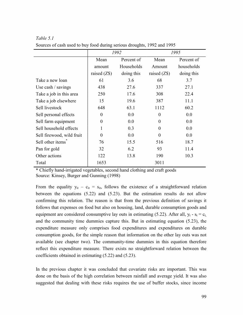
99

Table 5.1 Sources of cash used to buy food during serious droughts, 1992 and 1995 1992 1995 Mean

amount raised (Z$)

Percent of Households doing this

Mean Amount

raised (Z$)

Percent of households doing this

Take a new loan 61 3.6 68 3.7 Use cash / savings 438 27.6 337 27.1 Take a job in this area 250 17.6 308 22.4 Take a job elsewhere 15 19.6 387 11.1 Sell livestock 648 63.1 1112 60.2 Sell personal effects 0 0.0 0 0.0 Sell farm equipment 0 0.0 0 0.0 Sell household effects 1 0.3 0 0.0 Sell firewood, wild fruit 0 0.0 0 0.0 Sell other items* 76 15.5 516 18.7 Pan for gold 32 6.2 93 11.4 Other actions 122 13.8 190 10.3 Total 1653 3011 * Chiefly hand-irrigated vegetables, second hand clothing and craft goods Source: Kinsey, Burger and Gunning (1998) From the equality yit � cit = sit, follows the existence of a straightforward relation between the equations (5.22) and (5.23). But the estimation results do not allow confirming this relation. The reason is that from the previous definition of savings it follows that expenses on food but also on housing, land, durable consumption goods and equipment are considered consumptive lay outs in estimating (5.22). After all, yt - st = ct, and the community time dummies capture this. But in estimating equation (5.23), the expenditure measure only comprises food expenditures and expenditures on durable consumption goods, for the simple reason that information on the other lay outs was not available (see chapter two). The community-time dummies in this equation therefore reflect this expenditure measure. There exists no straightforward relation between the coefficients obtained in estimating (5.22) and (5.23). In the previous chapter it was concluded that covariate risks are important. This was done on the basis of the high correlation between rainfall and average yield. It was also suggested that dealing with these risks requires the use of buffer stocks, since income

100

pooling can only deal with idiosyncratic variations. If rainfall is indeed a source of aggregate risk, then this should show up in the data as a community level clustering in crop incomes and, given the agricultural nature of the economy and the limited possibilities for diversification, in total income as well. To explore this, crop and total income were regressed on village, time interacted, dummies. Table 5.2 reports the results for those observations (843 in total) included in the regressions of the next section. Because a case can be made for insurance to take place between individuals instead of between households, the table presents information on a per adult equivalent basis in the first two columns and on a household basis in the columns three and four. Statistically significant values of the regression�s F-test indicate that levels in (crop) income are more similar for those living in the same community than for those living in different communities.41 Regressing crop income on village-time interacted dummies, reported in the top half of table 5.2, yields high F-statistics implying that crop outcomes are indeed covariate, and underscoring the need to accumulate buffer stocks. This holds both at the household level and per adult equivalent, though the effect is somewhat stronger at the household level. Village effects become weaker if non-crop income is taken into account (reported in the second row). This is unsurprising. Already in chapter four the benefits of diversification were explored. Also from table 5.1 this may be concluded as in the face of a bad harvest, households compensate the loss of income by exploiting less preferred means to generate earnings. Where the F-statistics for incomes indicate the existence of covariate risks, our interest is in finding evidence for community level effects in consumption. Results are reported in the third row of table 5.2. There is no indication of greater similarities in consumption within villages than between villages. This may mean two things: little smoothing takes place within the village or the village is not the correct identity to define the insurance group. The three types of liquid assets are reported in rows four till six in table 5.2. Again there is evidence of community effects but the effect is weak, especially for cash savings. Still the presence of village effects in asset ownership suggests that some communities are better endowed than others. A similarly (weak) effect is found for livestock savings. The absence of a strong effect in savings need not imply the absence of full insurance as it is 41 This F-test tests for the absence of a relationship between the endogenous variable and the community-time dummies.

101

possible that within a given village only few households save for the benefit of the whole village. If this is what happens then differences between those within a community may be just as large as differences in savings between those in separate villages. Table 5.2 Regressing changes in income, crop income, savings and assets on village-time interacted dummies Dependent variable Per adult equivalent Household F-stat P-value F-stat P-value Crop Income 5.87 0.0000 11.00 0.0000 Total Income 3.95 0.0000 7.99 0.0000 Consumption 1.34 0.0643 1.30 0.0877 Cash balances 1.34 0.0652 1.47 0.0223 Livestock possessions 1.97 0.0001 3.34 0.0000 Grain stores 3.25 0.0000 3.99 0.0000 Livestock savings 2.36 0.0000 1.58 0.0081 F-stat P-value F-stat P-value ∆ Crop Income 3.94 0.0000 5.49 0.0000 ∆ Total Income 2.45 0.0000 2.72 0.0000 ∆ Consumption 1.39 0.0444 1.22 0.1499 ∆ Cash balances 1.01 0.4596 0.87 0.7159 ∆ Livestock possessions 2.05 0.0000 1.59 0.0895 ∆ Grain stores 3.05 0.0000 2.78 0.0000 ∆ Livestock savings 2.05 0.0000 2.00 0.0001

Source: estimated using Kinsey�s surveys. The test for full insurance does not test for comovement in levels but tests for comovement in first differences. These are reported in the bottom half of table 5.2. Clearly where village effects exist in levels, they are likely to appear in first differences as well. Measurement error may obscure these results however. Already in chapter three it was pointed out that especially for variables whose levels change little over time, the variance of measured changes may easily be dominated by measurement error, even if the measurement of the levels is relatively accurate. Measurement error appears to play a role as the F-tests for the changes in (crop) income, consumption, savings and assets are lower than for those in levels. Otherwise, the patterns are much the same. There is evidence for comovement in (crop) income, asset ownership and savings but there is

102

only a weak suggestion for comovement in consumption measured in adult equivalents. If one considers the differences in comovement between household level variables and variables expressed in adult equivalents then there is no reason to prefer one type of measure over the other.

5.4 Estimation Results

In the estimation 60 households were dropped because information on any of the variables was absent in any of the three years required to determine first differences. In total 139 communal households (out of a total of 150) and 351 resettled households (out of a total of 400) are included in the estimations. Not all reported private transfers were in cash and assigning a monetary value to these transfers turned out to be impossible. In order not to lose information it was decided to include additional variables in the estimations representing the quantity of items households received and provided.42 In the presence of full insurance, the inclusion of village dummies implies that endogeneity problems will not lead to biases in the estimates of the γ�s. To see why, suppose that an unobserved technology shock (e.g. draught animals have become stronger due to a new method of dipping) increases household income. In the absence of full insurance this increase in income could affect the consumption decision in two ways, (i) through a direct effect (income is higher) and (ii) because less assets are required for precautionary reasons. The latter suggests a correlation between the error term and household income so that in the presence of partial insurance the income coefficient would be biased. However, in the presence of full insurance, the household�s increase in income is captured in the dummy representing village endowments. If the household increases consumption it should be due to this increase in village endowments (and possibly the additional availability of endowments because the income process has become safer). Hence in the presence of full insurance the estimated γ�s will be unbiased (and equal to zero). Clearly this is not true if insurance is partial, in which case one would have to rely on instrumental variable techniques to deal with this kind of endogeneity.

42 Distinguished are agricultural inputs, maize, other food/home produce and other items, so that eight additional variables representing received respectively given were added to the regressions.

103

Another source of bias might come from measurement error. The worst kind affects both endogenous and exogenous variables, for instance if values have to be imputed to income or assets which are also used to determine consumption. Fortunately it was possible to establish expenditure and income and asset information using different questionnaire modules to obtain price and quantity information. So values that had to be imputed to deal with missing price information for consumption respectively income and measures could be derived from different sources. However if the variables in the model are expressed in adult equivalent terms, a new bias affecting variables on both sides of the regression is introduced if there is measurement error in household composition. To avoid this problem, and since in the previous section no good reasons were found to rely on per adult equivalent measures, the regressions are carried out at the household level. Still, in annex 5.2 an expenditure regression is presented capturing variables on a per capita basis.43 Even in the absence of a simultaneous measurement error between dependent and independent variables, measurement error in the explanatory variables remains an issue as it will lead to attenuation bias. Relying on instrumental variable estimation can solve this problem, but finding suitable instruments proved to be difficult. Using lagged values was not possible because, for communal households, all three available years of information were already used to calculate the first differences. Other instruments were discarded on economic grounds. One potential solution is to create instruments following the Durbin method (Kennedy, 1990). To do so the independent variables are ranked by size after which instrumental variables are defined by the rank order. This method, however, does not solve the measurement problem since it is unlikely that the true values of the different values would have the same rank order as the measured values. Rank order is therefore not a good instrument to deal with measurement error. In view of these problems and given the interest in testing for the presence of full insurance, it was decided to estimate equation (5.22) using OLS. The idea behind this approach is that if full insurance is rejected despite the presence of a downward attenuation bias, then it would certainly be rejected if the coefficients could have been estimated properly. The implication is however that if full insurance is rejected, the estimates for the coefficients are biased, due to measurement error and because of

43 The results in this regression are comparable to the ones presented in the main text. In the adult equivalent regression one additional variable, reflecting household composition, was included to capture the presence of economies of scale in household consumption (see Lanjouw and Ravallion (1995)).

104

endogeneity problems. So in the case of partial insurance, the coefficients do not have an interpretation. Table 5.3 presents the results for three estimations with village dummies. One for the sample as a whole and two comprising interaction terms. In one estimation interaction terms for poor households are incorporated; in the other interaction terms for households from communal areas are included. The coefficients for the change in income and the change in livestock endowments are positive in all three regressions. This is in accordance with the consumption rule presented in chapter four, where it was found that after a positive endowment shock (either assets or income) both consumption and savings increase. The coefficients for the different kinds of liquids assets are not identical, as we expected. Unlike livestock assets, cash balances enter the regression with a negative (and significant) sign. This underscores the earlier observation that in a highly inflationary environment, cash balances are kept for transaction reasons. And this is what the regression outcomes reflect. Grain stores are not significant. The regressions show no support for the presence of full insurance. T-tests that the coefficient for the change in income is equal to zero are rejected in each of the three regressions. This does not hold for changes in livestock endowments, which is insignificant and thereby in accordance with the suggestion of full insurance. The lack of significance may be a reflection of the fact that, unlike income or cash, livestock endowments are pooled at the village level. Or, it may be attributed to the absence of substantial changes in the levels of livestock possession, leading in the presence of measurement error to a low signal to noise ratios when estimating in first differences. In any case not only do the estimation reject the hypothesis of full insurance, absent insurance is also rejected, following the rejection of the hypothesis that village dummies are jointly zero. Next consider the differences in the degree of insurance between the poor and the non-poor. The estimation is also reported in table 5.3. As poor are considered those families owning less than half the median number of livestock in the year previous to the one for which complete information was obtained: 1996 (for land reform beneficiaries) and 1997 for communal households. The coefficients between both groups do not differ significantly so that the degree of insurance poor and the non-poor is identical. Given that the years for which these estimations were ran were characterised by relatively normal weather, this need not come as a surprise. After all, exclusion from existing insurance arrangements is most likely in situations with covariate shocks. Still, this

105

evidence diverges from Jalan and Ravallion (1999) who find different degrees of insurance between poor and non-poor households. No differences are found between communal and resettled households, implying either that the distrust effect is offset by the lack of privacy in the clustered villages or, and this seems more plausible, that after 20 years of resettlement the social cohesion (and possibilities for monitoring) between both groups of farmers has become comparable. The evidence rejects full insurance and is in favour of partial insurance. One reason why full insurance may be rejected is that the insurance group was improperly defined. After all, why would the village be the entity that confines the insurance group. Why for instance not consider the survey site as a whole? Therefore the regressions in table 5.3 were repeated, but now including survey site dummies. The results were essentially the same and are not presented here. It follows however that if full insurance exists nonetheless that the insurance group is not defined by administrative units like the village or the survey site. To further look into this issue it was considered who the providers and recipients of transfers are. Information to this end is presented in table 5.4. It shows the involvement of neighbours and friends in a quarter of all transfers. They are likely to be responsible for the evidence found for village level insurance. But most frequently mentioned as the recipient or provider of goods are family members. Some of them will live in the village itself but in many instances this will not be the case, explaining why insurance at the survey site level may work just as well as insurance at the village level. This suggests that if it had been possible to define as the relevant insurance group the village plus relatives living elsewhere, full insurance might not have been rejected. Unfortunately this could not be put to a test.44

44 Evidence of the importance of extra-village ties is presented by Grimard (1997) who reports for Côte d� Ivoire that people of same ethnic origin insure each other.

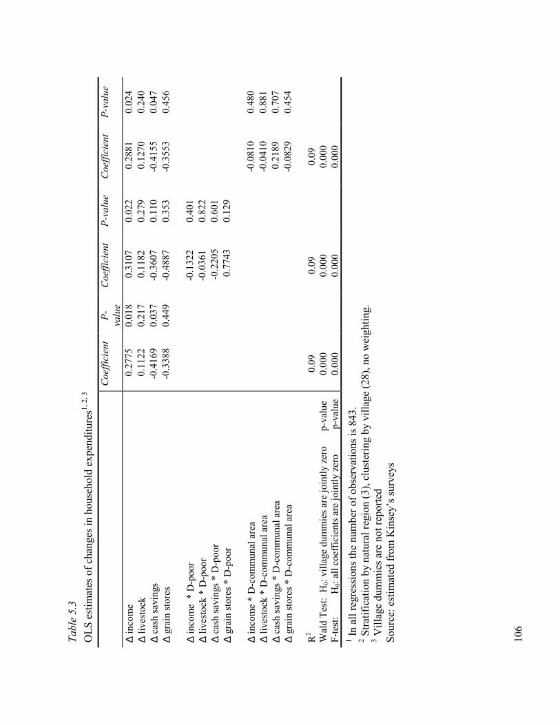
10

6

Tabl

e 5.

3 O

LS e

stim

ates

of c

hang

es in

hou

seho

ld e

xpen

ditu

res1,

2, 3

Co

effic

ient

P- valu

e Co

effic

ient

P-

valu

e Co

effic

ient

P-

valu

e

∆ in

com

e 0

.277

5 0.

018

0.3

107

0.02

2 0

.288

1 0.

024

∆ liv

esto

ck

0.1

122

0.21

7

0.1

182

0.27

9 0

.127

0 0.

240

∆ ca

sh sa

ving

s -0

.416

9 0.

037

-0.3

607

0.11

0 -0

.415

5 0.

047

∆ gr

ain

stor

es

-0.3

388

0.44

9 -0

.488

7 0.

353

-0.3

553

0.45

6

∆ in

com

e *

D-p

oor

-0.1

322

0.40

1

∆

lives

tock

* D

-poo

r

-0

.036

1 0.

822

∆ ca

sh sa

ving

s * D

-poo

r

-0

.220

5 0.

601

∆ gr

ain

stor

es *

D-p

oor

0.7

743

0.12

9

∆ in

com

e *

D-c

omm

unal

are

a

-0

.081

0 0.

480

∆ liv

esto

ck *

D-c

omm

unal

are

a

-0

.041

0 0.

881

∆ ca

sh sa

ving

s * D

-com

mun

al a

rea

0.2

189

0.70

7 ∆

grai

n st

ores

* D

-com

mun

al a

rea

-0.0

829

0.45

4

R2

0.09

0.09

0.09

Wal

d Te

st:

H0:

villa

ge d

umm

ies a

re jo

intly

zer

o

p-v

alue

0.

000

0.

000

0.

000

F-

test

:

H

0: al

l coe

ffic

ient

s are

join

tly z

ero

p-

valu

e 0.

000

0.

000

0.

000

1 In

all

regr

essi

ons t

he n

umbe

r of o

bser

vatio

ns is

843

. 2 S

tratif

icat

ion

by n

atur

al re

gion

(3),

clus

terin

g by

vill

age

(28)

, no

wei

ghtin

g.

3 Vill

age

dum

mie

s are

not

repo

rted

Sour

ce: e

stim

ated

from

Kin

sey�

s sur

veys

107

Table 5.4

Recipients / providers of private transfers in 1997 and 1998 Recipient / provider Parent of member of household 7% Child of member of household 27% Other blood relative 24% Relative related through marriage 13% Neighbour or friend 25% Other 4% 100% Source: calculated from Kinsey�s surveys

In section 5.2 it was also shown that instead of explaining expenditure, a full insurance test can also be based on the change in savings. A difficulty in estimating equation (5.23) is the possibility of correlations in measurement error between right and left hand side variables. After all, cash savings are imputed for differences in cash balances in subsequent years, implying that any measurement error in cash balances (included as exogenous variable) will be correlated with the measure for household savings (which includes cash savings). Again, instrumental variable estimation allows one to solve this issue but the absence of reliable instruments for both cash savings and food grain savings prevented doing so. One fortunate aspect is however that savings in livestock were determined independently from the level of livestock possession. So where it is not possible for the given data to estimate a complete savings function, it is possible to estimate a limited one, based on changes in cattle savings. And as cattle represent 76 percent of average household savings (and 87 percent in value terms) this regression is thought to be informative at least. It is included in annex 5.2. The results of this regression are comparable to the ones reported on the basis of table 5.3. Full insurance is rejected and so is the absence of all informal insurance.45 Another implication of the model presented in section 5.2 is that in the presence of full insurance the rank order of the different households should remain unchanged over time. This implication is already suggested by Banerjee and Newman (1991) but has not

45 Note that in this regression, the test on the presence of full insurance is whether the income coefficient is equal to one.

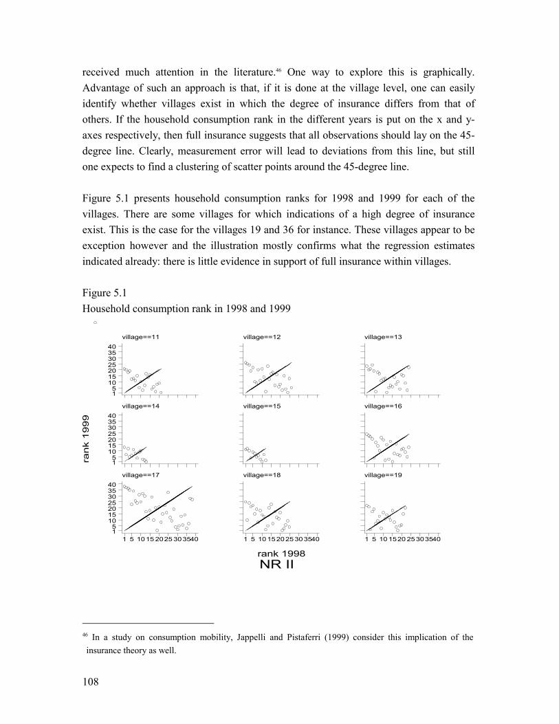
108

received much attention in the literature.46 One way to explore this is graphically. Advantage of such an approach is that, if it is done at the village level, one can easily identify whether villages exist in which the degree of insurance differs from that of others. If the household consumption rank in the different years is put on the x and y-axes respectively, then full insurance suggests that all observations should lay on the 45-degree line. Clearly, measurement error will lead to deviations from this line, but still one expects to find a clustering of scatter points around the 45-degree line. Figure 5.1 presents household consumption ranks for 1998 and 1999 for each of the villages. There are some villages for which indications of a high degree of insurance exist. This is the case for the villages 19 and 36 for instance. These villages appear to be exception however and the illustration mostly confirms what the regression estimates indicated already: there is little evidence in support of full insurance within villages. Figure 5.1 Household consumption rank in 1998 and 1999

ran

k 1

99

9

NR IIrank 1998

village==11

15

10152025303540

village==12 village==13

village==14

15

10152025303540

village==15 village==16

village==17

1 5 1015 2025 30354015

10152025303540

village==18

1 5 10 152025 303540

village==19

1 5 10 1520 25303540

46 In a study on consumption mobility, Jappelli and Pistaferri (1999) consider this implication of the insurance theory as well.

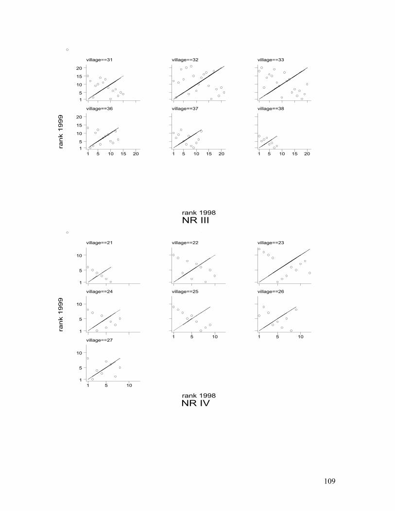
109

ran

k 1

99

9

NR IIIrank 1998

village==31

15

10

15

20

village==32 village==33

village==36

1 5 10 15 2015

10

15

20

village==37

1 5 10 15 20

village==38

1 5 10 15 20

ran

k 1

99

9

NR IVrank 1998

village==21

1

5

10

village==22 village==23

village==24

1

5

10

village==25

1 5 10

village==26

1 5 10village==27

1 5 101

5

10

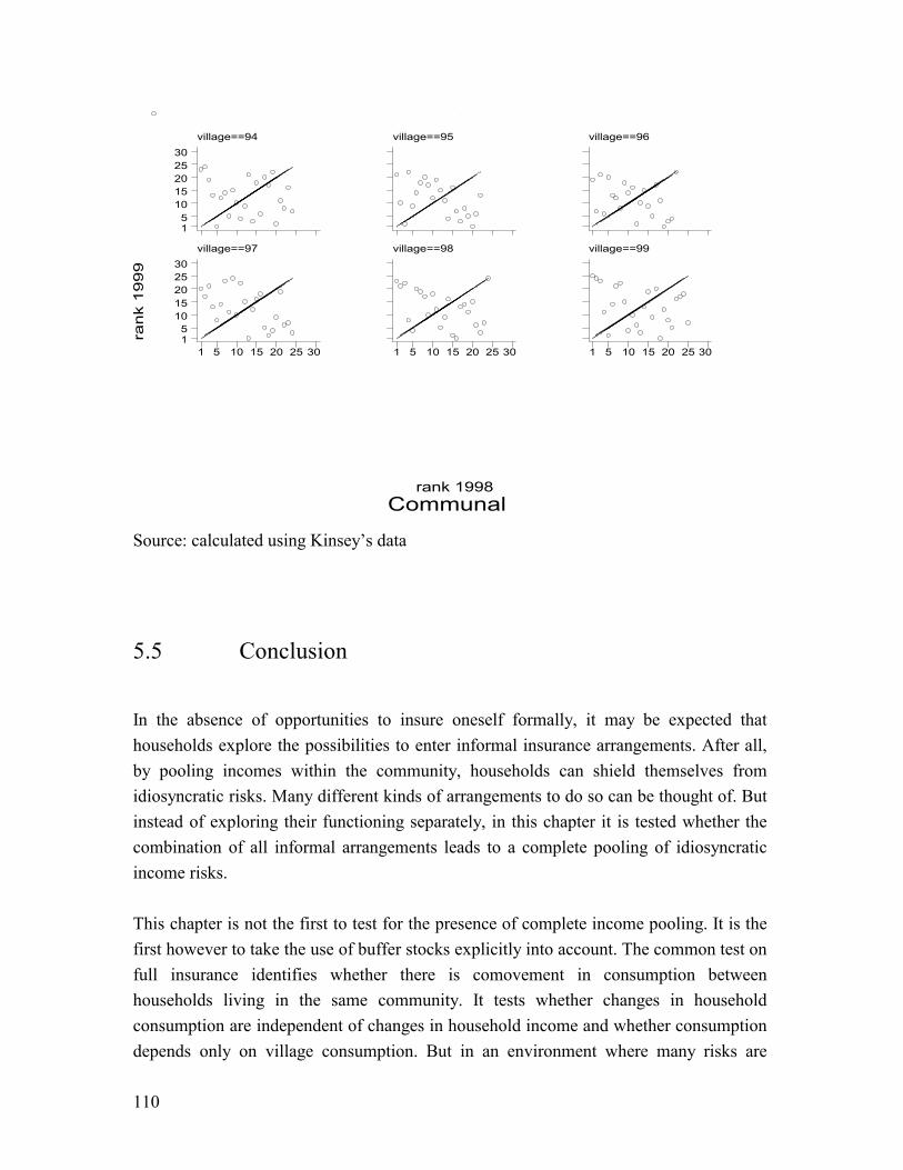
110

ran

k 1

99

9

Communalrank 1998

village==94

15

1015202530

village==95 village==96

village==97

1 5 10 15 20 25 3015

1015202530

village==98

1 5 10 15 20 25 30

village==99

1 5 10 15 20 25 30

Source: calculated using Kinsey�s data

5.5 Conclusion

In the absence of opportunities to insure oneself formally, it may be expected that households explore the possibilities to enter informal insurance arrangements. After all, by pooling incomes within the community, households can shield themselves from idiosyncratic risks. Many different kinds of arrangements to do so can be thought of. But instead of exploring their functioning separately, in this chapter it is tested whether the combination of all informal arrangements leads to a complete pooling of idiosyncratic income risks. This chapter is not the first to test for the presence of complete income pooling. It is the first however to take the use of buffer stocks explicitly into account. The common test on full insurance identifies whether there is comovement in consumption between households living in the same community. It tests whether changes in household consumption are independent of changes in household income and whether consumption depends only on village consumption. But in an environment where many risks are

111

covariate (and this chapter provided evidence to this end) and where households rely on buffer stocks to deal with them, such a test is inconclusive. The independence of household consumption from household income could also be brought about by relying on buffer stocks to attain a smooth consumption profile. After all, buffer stocks can be used to deal with covariate shocks but also to deal with idiosyncratic risks. However if changes in household consumption do not comove with changes in household income and household asset levels then this may be considered evidence for the presence of community level insurance. This point is formally illustrated in the theoretical part of this chapter. In the empirical part the presence of full insurance is put to a test. Evidence in support of full insurance was not found. This is an altogether unsurprising finding given the presence of information and incentive problems which hinder the functioning of informal insurance arrangements. But evidence in support of the reverse, complete absence of informal insurance arrangements, was not found either. Changes in household consumption (and savings) were found to be dependent not only on changes in household income but also on the village-time dummies. Two additional issues were explored: whether the poor are insured differently than the non-poor and whether differences in the degree of insurance exist between land reform beneficiaries and non-beneficiaries. With respect to the former, no support could be found for differences in the degree of insurance between poor and non-poor households. Also with respect to latter did the estimations not suggest the presence of differences between land reform beneficiaries and communal households.

Finally attention has been attributed to discovering what is the relevant insurance group. The degree of insurance was found to be similar, irrespective of whether village-time dummies or survey-site time dummies were included in the regressions. It follows that if full insurance exists that the insurance group would not be defined by administrative units like the village or the survey site. Indications were found that had it been possible to define the relevant insurance group as the village plus relatives living elsewhere, full insurance might not have been rejected.

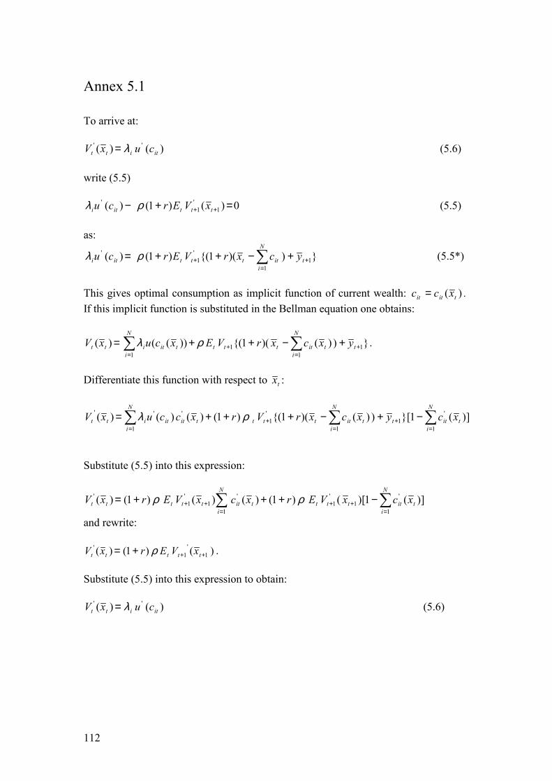
112

Annex 5.1 To arrive at:

)()( ''ititt cuxV λ= (5.6)

write (5.5)

0)()1()( 1'

1' =+− ++ tttiti xVErcu ρλ (5.5)

as:

}))(1{()1()( 11

'1

'+

=+ +−++= � t

N

iittttiti ycxrVErcu ρλ (5.5*)

This gives optimal consumption as implicit function of current wealth: )( titit xcc = . If this implicit function is substituted in the Bellman equation one obtains:

}))()(1{())(()( 11

11

+=

+=

+−++= �� t

N

ititttt

N

itititt yxcxrVExcuxV ρλ .

Differentiate this function with respect to tx :

])(1}[))()(1{()1()()()(1

'1

1

'1

1

'''���

=+

=+

=

−+−+++=N

ititt

N

ititttt

N

ititititt xcyxcxrVrxccuxV ρλ

Substitute (5.5) into this expression:

])(1)[()1()()()1()(1

'1

'1

1

'1

'1

'��

=++

=++ −+++=

N

ititttt

N

ititttttt xcxVErxcxVErxV ρρ

and rewrite:

)()1()( 1'

1'

+++= ttttt xVErxV ρ . Substitute (5.5) into this expression to obtain:

)()( ''ititt cuxV λ= (5.6)

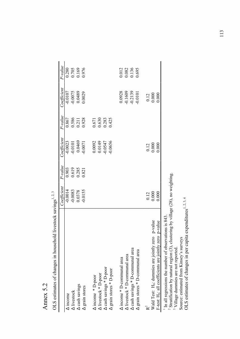
11

3

Ann

ex 5

.2

OLS

est

imat

es o

f cha

nges

in h

ouse

hold

live

stoc

k sa

ving

s1, 2

, 3

Co

effic

ient

P-

valu

e Co

effic

ient

P-

valu

e Co

effic

ient

P-

valu

e

∆ in

com

e -0

.001

4 0.

903

-0.0

023

0.86

7 -0

.010

7 0.

280

∆ liv

esto

ck

-0.0

083

0.61

9 -0

.010

1 0.

586

-0.0

075

0.70

5 ∆

cash

savi

ngs

0.03

78

0.28

5 0

.046

9 0.

211

0.0

489

0.16

9 ∆

grai

n st

ores

-0

.015

5 0.

821

-0.0

071

0.92

8 0.

0029

0.

976

∆

inco

me

* D

-poo

r

0

.009

2 0.

671

∆ liv

esto

ck *

D-p

oor

0.0

149

0.63

0

∆

cash

savi

ngs *

D-p

oor

-0.0

547

0.28

3

∆

grai

n st

ores

* D

-poo

r

-0

.065

6 0.

425

∆

inco

me

* D

-com

mun

al a

rea

0.0

928

0.01

2 ∆

lives

tock

* D

-com

mun

al a

rea

-0.1

609

0.08

2 ∆

cash

savi

ngs *

D-c

omm

unal

are

a

-0

.213

9 0.

136

∆ gr

ain

stor

es *

D-c

omm

unal

are

a

-0

.010

1 0.

695

R

2 0.

12

0.

12

0.

12

W

ald

Test

: H

0: du

mm

ies a

re jo

intly

zer

o p

-val

ue

0.00

0

0.00

0

0.00

0

F-te

st: H

0: al

l coe

ffic

ient

s are

join

tly z

ero

p-v

alue

0.

000

0.

000

0.

000

1 In

all

regr

essi

ons t

he n

umbe

r of o

bser

vatio

ns is

843

. 2 S

tratif

icat

ion

by n

atur

al re

gion

(3),

clus

terin

g by

vill

age

(28)

, no

wei

ghtin

g.

3 Vill

age

dum

mie

s are

not

repo

rted.

So

urce

: est

imat

ed fr

om K

inse

y�s s

urve

ys

OLS

est

imat

es o

f cha

nges

in p

er c

apita

exp

endi

ture

s1, 2

, 3, 4

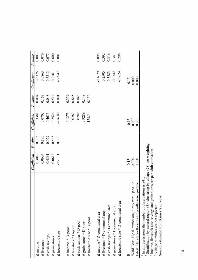
11

4

Co

effic

ient

P-

valu

e Co

effic

ient

P-

valu

e Co

effic

ient

P-

valu

e

∆ in

com

e 0.

3019

0.

003

0.33

81

0.00

4 0.

3375

0.

003

∆ liv

esto

ck

0.06

04

0.13

6 0.

0702

0.

168

0.08

63

0.07

0 ∆

cash

savi

ngs

-0.4

561

0.02

9 -0

.463

3 0.

048

-0.5

213

0.07

7 ∆

grai

n st

ores

-0

.061

3 0.

863

-0.2

526

0.51

4 -0

.216

1 0.

600

∆ ho

useh

old

size

-2

51.3

1 0.

000

-216

.89

0.00

1 -2

23.4

7 0.

001

∆

inco

me

* D

-poo

r

-0

.137

3 0.

359

∆ liv

esto

ck *

D-p

oor

-0.0

287

0.64

5

∆

cash

savi

ngs *

D-p

oor

0.07

89

0.84

5

∆

grai

n st

ores

* D

-poo

r

0.

9289

0.

148

∆ ho

useh

old

size

* D

-poo

r

-1

73.5

4 0.

150

∆

inco

me

* D

-com

mun

al a

rea

-0.1

629

0.09

5 ∆

lives

tock

* D

-com

mun

al a

rea

0.25

05

0.39

2 ∆

cash

savi

ngs *

D-c

omm

unal

are

a

0.

5283

0.

316

∆ gr

ain

stor

es *

D-c

omm

unal

are

a

-0

.074

2 0.

347

∆ ho

useh

old

size

* D

-com

mun

al a

rea

-268

.24

0.29

6

R2

0.15

0.15

0.15

Wal

d Te

st:

H0:

dum

mie

s are

join

tly z

ero

p-v

alue

0.

000

0.

000

0.

000

F-

test

: H0:

all c

oeff

icie

nts a

re jo

intly

zer

o p

-val

ue

0.00

0

0.00

0

0.00

0

1 In a

ll re

gres

sion

s the

num

ber o

f obs

erva

tions

is 8

41.

2 Stra

tific

atio

n by

nat

ural

regi

on (3

), cl

uste

ring

by v

illag

e (2

8), n

o w

eigh

ting.

3 In

com

e, li

vest

ock

cash

savi

ngs a

nd g

rain

stor

es a

re p

er a

dult

equi

vale

nt.

4 Vill

age

dum

mie

s are

not

repo

rted

Sour

ce: e

stim

ated

from

Kin

sey�

s sur

veys

Cattle as Source of Risk

6.1 Introduction47 In the two preceding chapters possessing cattle contributed to household security. In this chapter cattle are shown to be a source of risk. More specifically the possession of a span of draught animals is shown to be a prerequisite to earning a good income from agriculture. For those possessing insufficient animals, even the possibility of getting stuck in a poverty trap cannot be excluded. Since everybody runs the risk of losing one�s animals, the mere existence of a poverty trap is reason to consider insurance arrangements focussed on livestock. An illustration of such an arrangement will be provided in the next chapter. This chapter is therefore a bridge between the role cattle play in consumption smoothing (by being a buffer stock) and informal insurance arrangements focused on cattle. This chapter is not the first in suggesting that households may end up in a poverty trap. Eswaran and Kotwal (1986), Galor and Zeira (1993), Banerjee and Newman (1993) and Aghion and Bolton (1997) present theoretical papers where due to an inequitable initial distribution of resources in combination with imperfect credit markets and non-convexities in the production technology, only the wealthier

116

households are able to take up a profitable activity.48 This in turn allows the already well off to grow richer while other households remain in poverty. In an effort to show that all households are vulnerable to such a situation, Dasgupta and Ray (1986) postulate a non-convexity in the provision of labour by making it dependent on whether food intake exceeds a minimum threshold.49 In this chapter it is argued that not the minimum level of nutrition but the need for at least two draught animals is a non-convexity making Zimbabwean smallholder farmers subject to the risk of a poverty trap. The reason for this is that those who prepare their land for cultivation manually are unable to save enough to obtain the resources required to buy traction animals. Empirical evidence to support this claim is provided. The organisation of the chapter is as follows. In the next section attention is paid to the production technology used by Zimbabwean smallholder farmers and the importance of cattle therein. In section 6.3 it is derived theoretically how, in the absence of credit and cattle rental markets, the need for a team of draught animals may lead to a poverty trap. In section 6.4 the predictions of the model with respect to the distribution of draught animals are verified. In section 6.5 empirical evidence for the existence of the non-convexity in the production technology is presented. Conclusions follow in 6.6.

47 The model presented in this chapter was published in Tijdschrift voor Politieke Economie 22: 82-104 (1999).

48 Eswaran and Kotwal (1986) postulate the existence of fixed set up costs in agricultural cultivation and show that if credit constraints are linked to collateral requirements and if land can be used as collateral, then households with relatively low land endowments may not be able to cultivate all their land and instead will rent out some of their labour to households with larger land holdings. Galor and Zeira (1993) emphasise the role of a non-convex production technology where the credit constrained poor family cannot overcome the minimum threshold size for investment in human capital. Banerjee and Newman (1993) show that poor people who are unable to afford the collateral required to be self-employed entrepreneurs or employers crowd the labour market and depress the wage rate and thereby the bequest they leave for their children; Aghion and Bolton (1997) focus on the capital market and the relationship between wealth inequality and the cost of borrowing and hence access to investment opportunities for the poor.

49 Srinivasan (1994) considers Dasgupta and Ray�s suggestion unrealistic. He points out that: �in India the cost of food containing adequate energy at the prevailing prices is surprisingly modest at an individual level, less than ten percent of the unskilled wage rate. [�] If this is the case, it would seem that an explanation for the persistence of destitution has to be sought, not in a nutrition based theory of resource allocation [�] � (p. 1854).

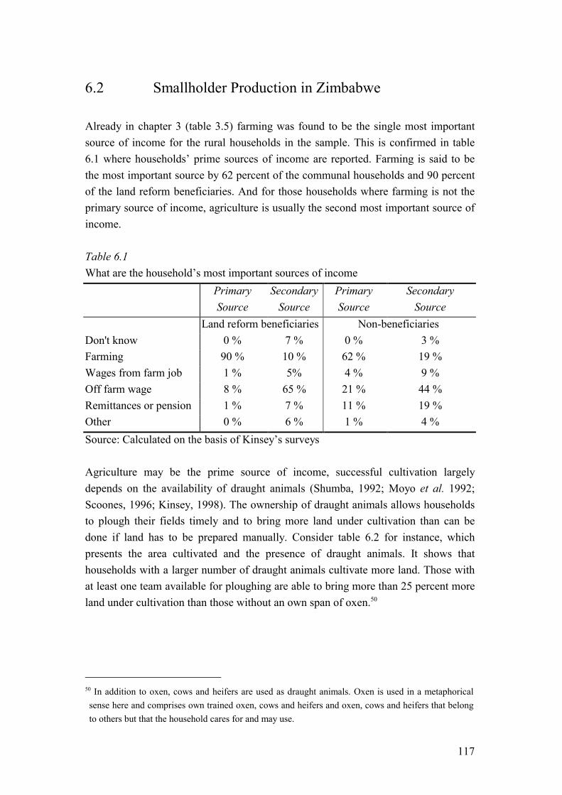
117

6.2 Smallholder Production in Zimbabwe Already in chapter 3 (table 3.5) farming was found to be the single most important source of income for the rural households in the sample. This is confirmed in table 6.1 where households� prime sources of income are reported. Farming is said to be the most important source by 62 percent of the communal households and 90 percent of the land reform beneficiaries. And for those households where farming is not the primary source of income, agriculture is usually the second most important source of income. Table 6.1 What are the household�s most important sources of income Primary

Source Secondary

Source Primary Source

Secondary Source

Land reform beneficiaries Non-beneficiaries Don't know 0 % 7 % 0 % 3 % Farming 90 % 10 % 62 % 19 % Wages from farm job 1 % 5% 4 % 9 % Off farm wage 8 % 65 % 21 % 44 % Remittances or pension 1 % 7 % 11 % 19 % Other 0 % 6 % 1 % 4 % Source: Calculated on the basis of Kinsey�s surveys Agriculture may be the prime source of income, successful cultivation largely depends on the availability of draught animals (Shumba, 1992; Moyo et al. 1992; Scoones, 1996; Kinsey, 1998). The ownership of draught animals allows households to plough their fields timely and to bring more land under cultivation than can be done if land has to be prepared manually. Consider table 6.2 for instance, which presents the area cultivated and the presence of draught animals. It shows that households with a larger number of draught animals cultivate more land. Those with at least one team available for ploughing are able to bring more than 25 percent more land under cultivation than those without an own span of oxen.50

50 In addition to oxen, cows and heifers are used as draught animals. Oxen is used in a metaphorical sense here and comprises own trained oxen, cows and heifers and oxen, cows and heifers that belong to others but that the household cares for and may use.

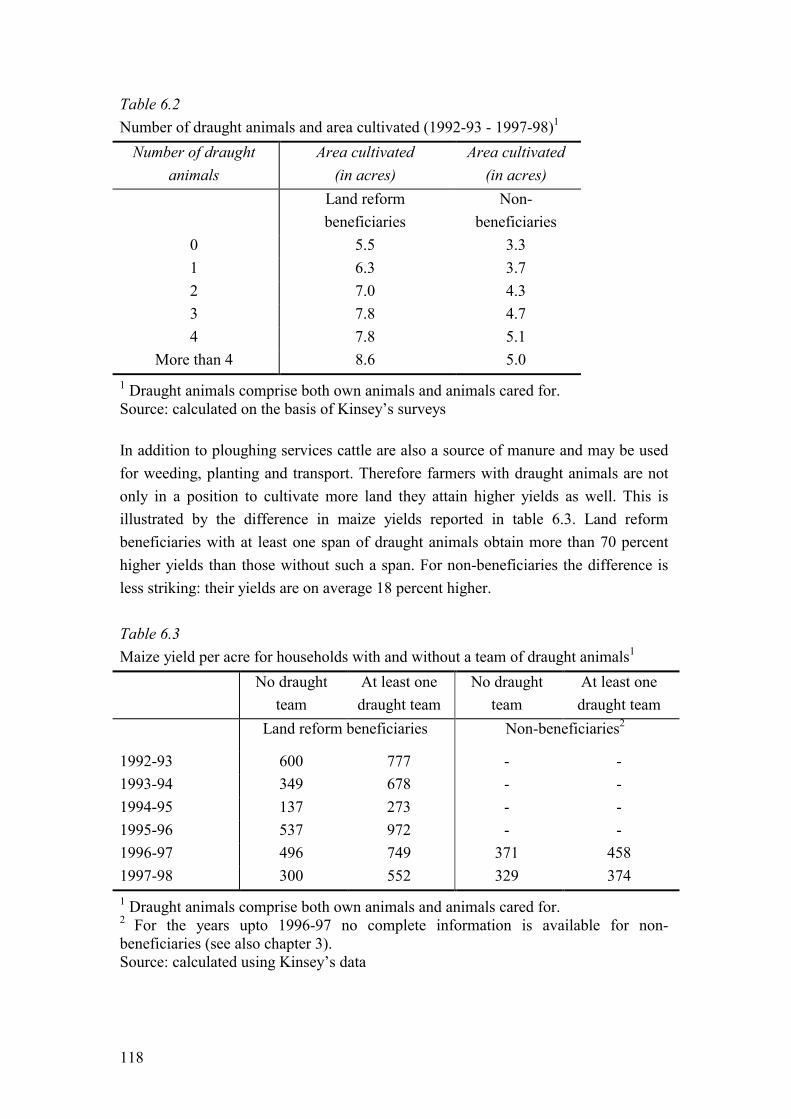
118

Table 6.2 Number of draught animals and area cultivated (1992-93 - 1997-98)1

Number of draught animals

Area cultivated (in acres)

Area cultivated (in acres)

Land reform beneficiaries

Non-beneficiaries

0 5.5 3.3 1 6.3 3.7 2 7.0 4.3 3 7.8 4.7 4 7.8 5.1

More than 4 8.6 5.0

1 Draught animals comprise both own animals and animals cared for. Source: calculated on the basis of Kinsey�s surveys In addition to ploughing services cattle are also a source of manure and may be used for weeding, planting and transport. Therefore farmers with draught animals are not only in a position to cultivate more land they attain higher yields as well. This is illustrated by the difference in maize yields reported in table 6.3. Land reform beneficiaries with at least one span of draught animals obtain more than 70 percent higher yields than those without such a span. For non-beneficiaries the difference is less striking: their yields are on average 18 percent higher. Table 6.3 Maize yield per acre for households with and without a team of draught animals1

No draught team

At least one draught team

No draught team

At least one draught team

Land reform beneficiaries Non-beneficiaries2

1992-93 600 777 - - 1993-94 349 678 - - 1994-95 137 273 - - 1995-96 537 972 - - 1996-97 496 749 371 458 1997-98 300 552 329 374

1 Draught animals comprise both own animals and animals cared for. 2 For the years upto 1996-97 no complete information is available for non-beneficiaries (see also chapter 3). Source: calculated using Kinsey�s data

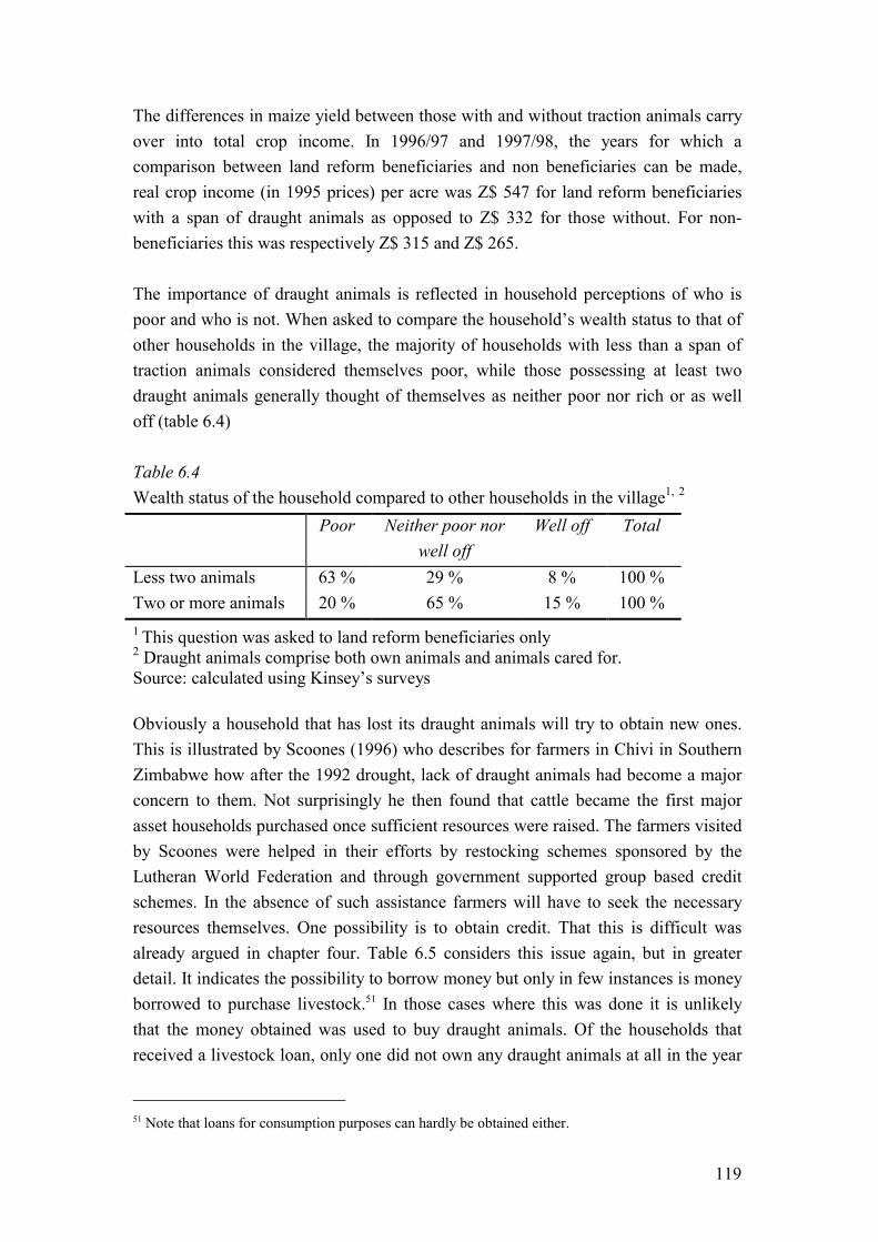
119

The differences in maize yield between those with and without traction animals carry over into total crop income. In 1996/97 and 1997/98, the years for which a comparison between land reform beneficiaries and non beneficiaries can be made, real crop income (in 1995 prices) per acre was Z$ 547 for land reform beneficiaries with a span of draught animals as opposed to Z$ 332 for those without. For non-beneficiaries this was respectively Z$ 315 and Z$ 265. The importance of draught animals is reflected in household perceptions of who is poor and who is not. When asked to compare the household�s wealth status to that of other households in the village, the majority of households with less than a span of traction animals considered themselves poor, while those possessing at least two draught animals generally thought of themselves as neither poor nor rich or as well off (table 6.4) Table 6.4 Wealth status of the household compared to other households in the village1, 2

Poor Neither poor nor well off

Well off Total

Less two animals 63 % 29 % 8 % 100 % Two or more animals 20 % 65 % 15 % 100 %

1 This question was asked to land reform beneficiaries only 2 Draught animals comprise both own animals and animals cared for. Source: calculated using Kinsey�s surveys Obviously a household that has lost its draught animals will try to obtain new ones. This is illustrated by Scoones (1996) who describes for farmers in Chivi in Southern Zimbabwe how after the 1992 drought, lack of draught animals had become a major concern to them. Not surprisingly he then found that cattle became the first major asset households purchased once sufficient resources were raised. The farmers visited by Scoones were helped in their efforts by restocking schemes sponsored by the Lutheran World Federation and through government supported group based credit schemes. In the absence of such assistance farmers will have to seek the necessary resources themselves. One possibility is to obtain credit. That this is difficult was already argued in chapter four. Table 6.5 considers this issue again, but in greater detail. It indicates the possibility to borrow money but only in few instances is money borrowed to purchase livestock.51 In those cases where this was done it is unlikely that the money obtained was used to buy draught animals. Of the households that received a livestock loan, only one did not own any draught animals at all in the year

51 Note that loans for consumption purposes can hardly be obtained either.

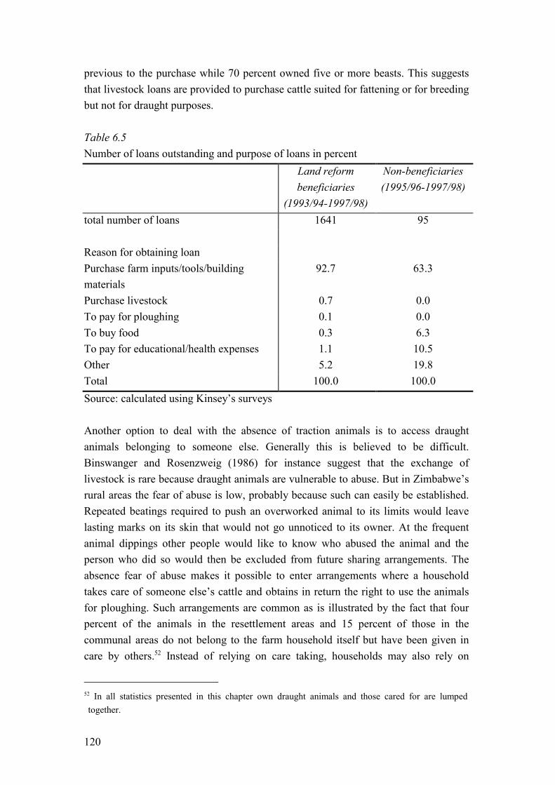
120

previous to the purchase while 70 percent owned five or more beasts. This suggests that livestock loans are provided to purchase cattle suited for fattening or for breeding but not for draught purposes. Table 6.5 Number of loans outstanding and purpose of loans in percent Land reform

beneficiaries (1993/94-1997/98)

Non-beneficiaries (1995/96-1997/98)

total number of loans 1641 95 Reason for obtaining loan Purchase farm inputs/tools/building materials

92.7 63.3

Purchase livestock 0.7 0.0 To pay for ploughing 0.1 0.0 To buy food 0.3 6.3 To pay for educational/health expenses 1.1 10.5 Other 5.2 19.8 Total 100.0 100.0 Source: calculated using Kinsey�s surveys Another option to deal with the absence of traction animals is to access draught animals belonging to someone else. Generally this is believed to be difficult. Binswanger and Rosenzweig (1986) for instance suggest that the exchange of livestock is rare because draught animals are vulnerable to abuse. But in Zimbabwe�s rural areas the fear of abuse is low, probably because such can easily be established. Repeated beatings required to push an overworked animal to its limits would leave lasting marks on its skin that would not go unnoticed to its owner. At the frequent animal dippings other people would like to know who abused the animal and the person who did so would then be excluded from future sharing arrangements. The absence fear of abuse makes it possible to enter arrangements where a household takes care of someone else�s cattle and obtains in return the right to use the animals for ploughing. Such arrangements are common as is illustrated by the fact that four percent of the animals in the resettlement areas and 15 percent of those in the communal areas do not belong to the farm household itself but have been given in care by others.52 Instead of relying on care taking, households may also rely on

52 In all statistics presented in this chapter own draught animals and those cared for are lumped together.

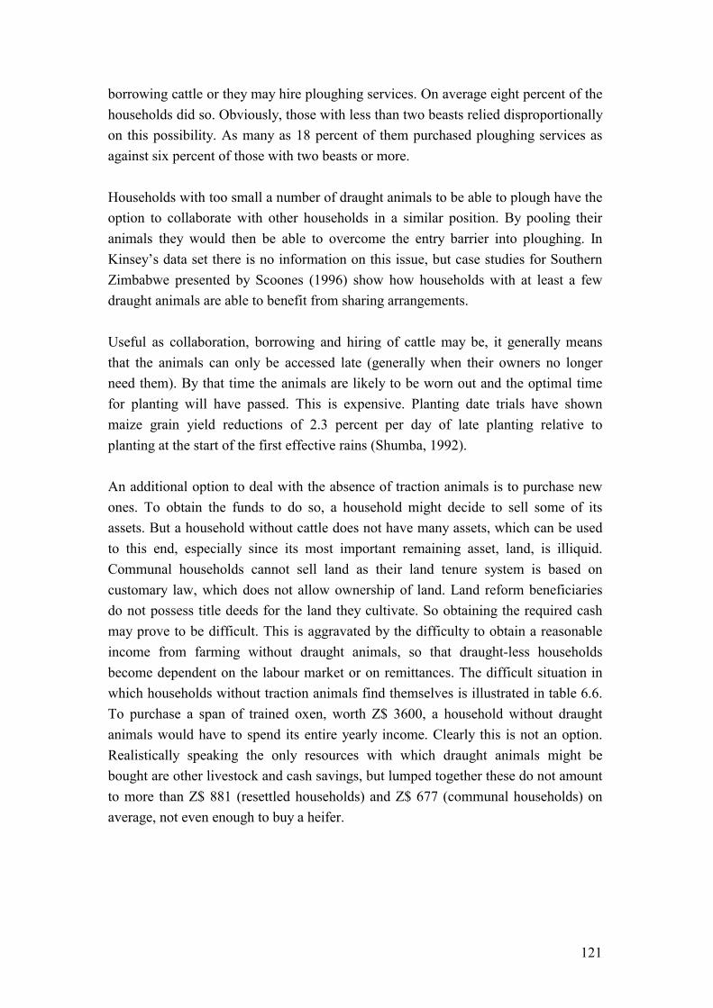
121

borrowing cattle or they may hire ploughing services. On average eight percent of the households did so. Obviously, those with less than two beasts relied disproportionally on this possibility. As many as 18 percent of them purchased ploughing services as against six percent of those with two beasts or more. Households with too small a number of draught animals to be able to plough have the option to collaborate with other households in a similar position. By pooling their animals they would then be able to overcome the entry barrier into ploughing. In Kinsey�s data set there is no information on this issue, but case studies for Southern Zimbabwe presented by Scoones (1996) show how households with at least a few draught animals are able to benefit from sharing arrangements. Useful as collaboration, borrowing and hiring of cattle may be, it generally means that the animals can only be accessed late (generally when their owners no longer need them). By that time the animals are likely to be worn out and the optimal time for planting will have passed. This is expensive. Planting date trials have shown maize grain yield reductions of 2.3 percent per day of late planting relative to planting at the start of the first effective rains (Shumba, 1992). An additional option to deal with the absence of traction animals is to purchase new ones. To obtain the funds to do so, a household might decide to sell some of its assets. But a household without cattle does not have many assets, which can be used to this end, especially since its most important remaining asset, land, is illiquid. Communal households cannot sell land as their land tenure system is based on customary law, which does not allow ownership of land. Land reform beneficiaries do not possess title deeds for the land they cultivate. So obtaining the required cash may prove to be difficult. This is aggravated by the difficulty to obtain a reasonable income from farming without draught animals, so that draught-less households become dependent on the labour market or on remittances. The difficult situation in which households without traction animals find themselves is illustrated in table 6.6. To purchase a span of trained oxen, worth Z$ 3600, a household without draught animals would have to spend its entire yearly income. Clearly this is not an option. Realistically speaking the only resources with which draught animals might be bought are other livestock and cash savings, but lumped together these do not amount to more than Z$ 881 (resettled households) and Z$ 677 (communal households) on average, not even enough to buy a heifer.

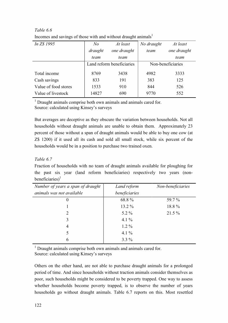
122

Table 6.6 Incomes and savings of those with and without draught animals1

In Z$ 1995 No draught

team

At least one draught

team

No draught team

At least one draught

team Land reform beneficiaries Non-beneficiaries

Total income 8769 3438 4982 3333 Cash savings 833 191 383 125 Value of food stores 1533 910 844 526 Value of livestock 14827 690 9770 552

1 Draught animals comprise both own animals and animals cared for. Source: calculated using Kinsey�s surveys But averages are deceptive as they obscure the variation between households. Not all households without draught animals are unable to obtain them. Approximately 23 percent of those without a span of draught animals would be able to buy one cow (at Z$ 1200) if it used all its cash and sold all small stock, while six percent of the households would be in a position to purchase two trained oxen. Table 6.7 Fraction of households with no team of draught animals available for ploughing for the past six year (land reform beneficiaries) respectively two years (non-beneficiaries)1

Number of years a span of draught animals was not available

Land reform beneficiaries

Non-beneficiaries

0 68.8 % 59.7 % 1 13.2 % 18.8 % 2 5.2 % 21.5 % 3 4.1 % 4 1.2 % 5 4.1 % 6 3.3 %

1 Draught animals comprise both own animals and animals cared for. Source: calculated using Kinsey�s surveys Others on the other hand, are not able to purchase draught animals for a prolonged period of time. And since households without traction animals consider themselves as poor, such households might be considered to be poverty trapped. One way to assess whether households become poverty trapped, is to observe the number of years households go without draught animals. Table 6.7 reports on this. Most resettled

123

households, 69 percent, possessed at least one span of draught animals during each of the six survey years. But a substantial fraction (almost 20 percent) went without draught animals for at least one or two years. And seven percent had less than two beasts in five or six of the survey years covered. These latter households might be considered to be stuck in poverty. For the communal households less information is available, but already on the basis of the two years for which complete information is available the percentage of households without outline animals for two years is substantially higher than the fraction of land reform beneficiaries without draught animals in two of the six years for which information is available. This suggests that communal households are substantially worse off. On the other hand, they are also less dependent upon agriculture and more integrated in the labour market so that the absence of draught animals might affect them less.53 In conclusion cattle are important to earn a good income from agriculture. Households without a span of draught animals plant fewer acres and obtain lower yields per acre. As a result they obtain low incomes. Taking care of someone else�s cattle is possible and sharing and hiring arrangements exist, but these responses cannot prevent that households without a team of oxen obtain low income from farming. Once lost, obtaining new beasts is difficult precisely because of the difficulty to obtain a reasonable income from agriculture in the absence of a span of draught animals. Especially for the land reform beneficiaries going without draught animals is problematic, as they are almost entirely dependent upon agriculture. Some land reform beneficiaries without traction animals were unable to obtain oxen for a long period of time. They may be considered poverty trapped. Going without draught animals is even a more serious problem for communal households but they rely to a much greater extent on off farm sources of income.

6.3 Deriving a Livestock Induced Poverty Trap The stylised facts behind the model, which will be developed in this section fit the description presented above and are typical for rural African households in general (Binswanger and McIntire, 1987; Platteau, 1999). These are: • Credit and land markets are absent.

53 It is not clear in this case what is the direction of causality, whether communal households are more integrated in the labour market because of the limited opportunities in farming, or whether they pay less attention to farming because of the good opportunities in the labour market.

124

• The market for draught services is imperfect. • Plots are sufficiently large so make the use of traction animals attractive. • There is a technological non-convexity in land preparation. Consider a rural household in an environment where cattle are important. Cattle can be slaughtered and consumed, or they can be used as draught animals. To use cattle for the latter purpose a minimum number is required, preferably two (or more) oxen, though combinations of trained oxen and other cattle are also possible. Otherwise, field preparation is done by hand. So, the choice is between two technologies, one allowing the farmer to cultivate a large area of land, ox-ploughing, and one confining him to a smaller acreage: manual preparation. The household offers labour in a fixed amount, which is normalised to one. It cultivates a plot of not transferable land which is sufficiently large to make the use of traction animals viable. Production per unit of land is constant and normalised to one. Hence total output is fully determined by the area of land ploughed. The household chooses the most profitable deterministic production technology depending on the availability of draught animals. If the household possesses less than the threshold level of capital, K , then it cultivates a fixed amount of land y . Households with sufficient capital prepare at least an amount of land equal to z, ( yz ≥ ) and if the number of draught animals exceeds the minimum number required, then more land is brought under cultivation. There is a constant marginal return α to draught animals exceeding the threshold level to reflect that with more draught animals available, animals become less tired if they work in spans of multiples of two, or, if they interchange each other at the yoke. The return is assumed to be constant for ease of modelling, but in fact with land and labour availability fixed the marginal return to capital is likely to be diminishing. The production choice is described by:

],max[ *'ttt yyy = (6.1)

with for KKt <−1 : yy t ='

and for KKt ≥−1 : 0,)( 1

* >≥−+= − αα yzKKzy tt

where y, z, α and K are constants, yt is the area of land prepared, being either yt

' or

yt* depending on whether the household attained the threshold level K for

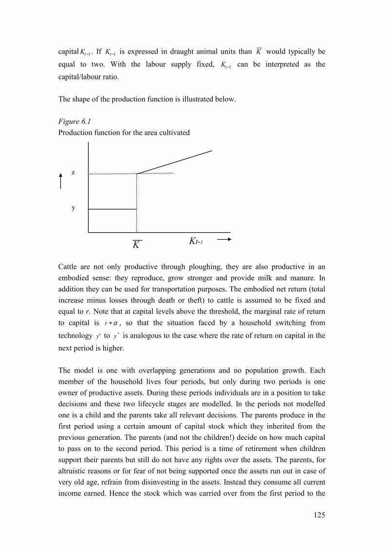
125

capital 1−tK . If 1−tK is expressed in draught animal units than K would typically be equal to two. With the labour supply fixed, 1−tK can be interpreted as the capital/labour ratio. The shape of the production function is illustrated below. Figure 6.1 Production function for the area cultivated Cattle are not only productive through ploughing, they are also productive in an embodied sense: they reproduce, grow stronger and provide milk and manure. In addition they can be used for transportation purposes. The embodied net return (total increase minus losses through death or theft) to cattle is assumed to be fixed and equal to r. Note that at capital levels above the threshold, the marginal rate of return to capital is r +α , so that the situation faced by a household switching from technology y' to y * is analogous to the case where the rate of return on capital in the next period is higher. The model is one with overlapping generations and no population growth. Each member of the household lives four periods, but only during two periods is one owner of productive assets. During these periods individuals are in a position to take decisions and these two lifecycle stages are modelled. In the periods not modelled one is a child and the parents take all relevant decisions. The parents produce in the first period using a certain amount of capital stock which they inherited from the previous generation. The parents (and not the children!) decide on how much capital to pass on to the second period. This period is a time of retirement when children support their parents but still do not have any rights over the assets. The parents, for altruistic reasons or for fear of not being supported once the assets run out in case of very old age, refrain from disinvesting in the assets. Instead they consume all current income earned. Hence the stock which was carried over from the first period to the

y

z

Kt-1K

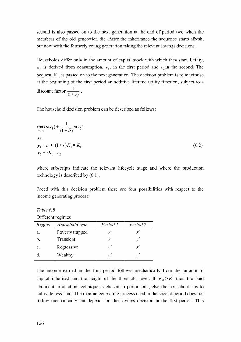
126

second is also passed on to the next generation at the end of period two when the members of the old generation die. After the inheritance the sequence starts afresh, but now with the formerly young generation taking the relevant savings decisions. Households differ only in the amount of capital stock with which they start. Utility, u , is derived from consumption, c1 , in the first period and c2 in the second. The bequest, K1, is passed on to the next generation. The decision problem is to maximise at the beginning of the first period an additive lifetime utility function, subject to a

discount factor 11( )+δ

.

The household decision problem can be described as follows:

212

1011

21

)1(..

)()1(

1)(max21

crKyKKrcy

ts

cucucc

=+=++−

++

δ

(6.2)

where subscripts indicate the relevant lifecycle stage and where the production technology is described by (6.1). Faced with this decision problem there are four possibilities with respect to the income generating process: Table 6.8 Different regimes Regime Household type Period 1 period 2 a. Poverty trapped y' y' b. Transient y' y * c. Regressive y * y'

d. Wealthy y * y *

The income earned in the first period follows mechanically from the amount of capital inherited and the height of the threshold level. If KK >0 then the land

abundant production technique is chosen in period one, else the household has to cultivate less land. The income generating process used in the second period does not follow mechanically but depends on the savings decision in the first period. This

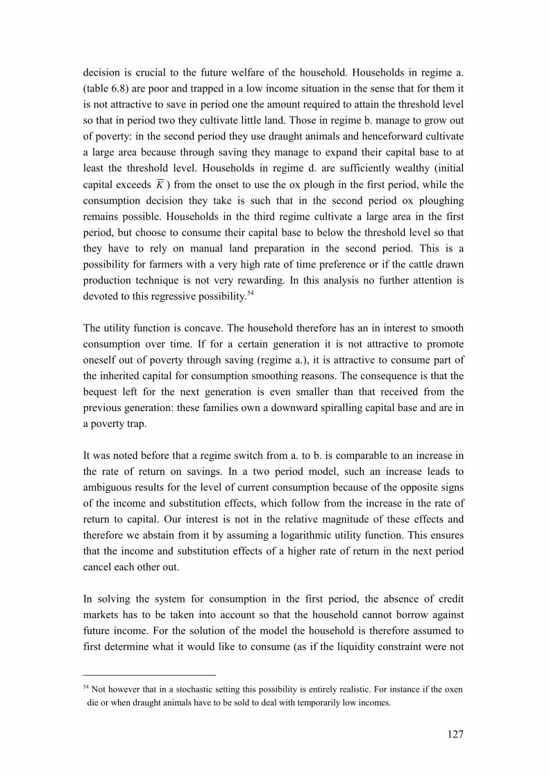
127

decision is crucial to the future welfare of the household. Households in regime a. (table 6.8) are poor and trapped in a low income situation in the sense that for them it is not attractive to save in period one the amount required to attain the threshold level so that in period two they cultivate little land. Those in regime b. manage to grow out of poverty: in the second period they use draught animals and henceforward cultivate a large area because through saving they manage to expand their capital base to at least the threshold level. Households in regime d. are sufficiently wealthy (initial capital exceeds K ) from the onset to use the ox plough in the first period, while the consumption decision they take is such that in the second period ox ploughing remains possible. Households in the third regime cultivate a large area in the first period, but choose to consume their capital base to below the threshold level so that they have to rely on manual land preparation in the second period. This is a possibility for farmers with a very high rate of time preference or if the cattle drawn production technique is not very rewarding. In this analysis no further attention is devoted to this regressive possibility.54 The utility function is concave. The household therefore has an in interest to smooth consumption over time. If for a certain generation it is not attractive to promote oneself out of poverty through saving (regime a.), it is attractive to consume part of the inherited capital for consumption smoothing reasons. The consequence is that the bequest left for the next generation is even smaller than that received from the previous generation: these families own a downward spiralling capital base and are in a poverty trap. It was noted before that a regime switch from a. to b. is comparable to an increase in the rate of return on savings. In a two period model, such an increase leads to ambiguous results for the level of current consumption because of the opposite signs of the income and substitution effects, which follow from the increase in the rate of return to capital. Our interest is not in the relative magnitude of these effects and therefore we abstain from it by assuming a logarithmic utility function. This ensures that the income and substitution effects of a higher rate of return in the next period cancel each other out. In solving the system for consumption in the first period, the absence of credit markets has to be taken into account so that the household cannot borrow against future income. For the solution of the model the household is therefore assumed to first determine what it would like to consume (as if the liquidity constraint were not

54 Not however that in a stochastic setting this possibility is entirely realistic. For instance if the oxen die or when draught animals have to be sold to deal with temporarily low incomes.

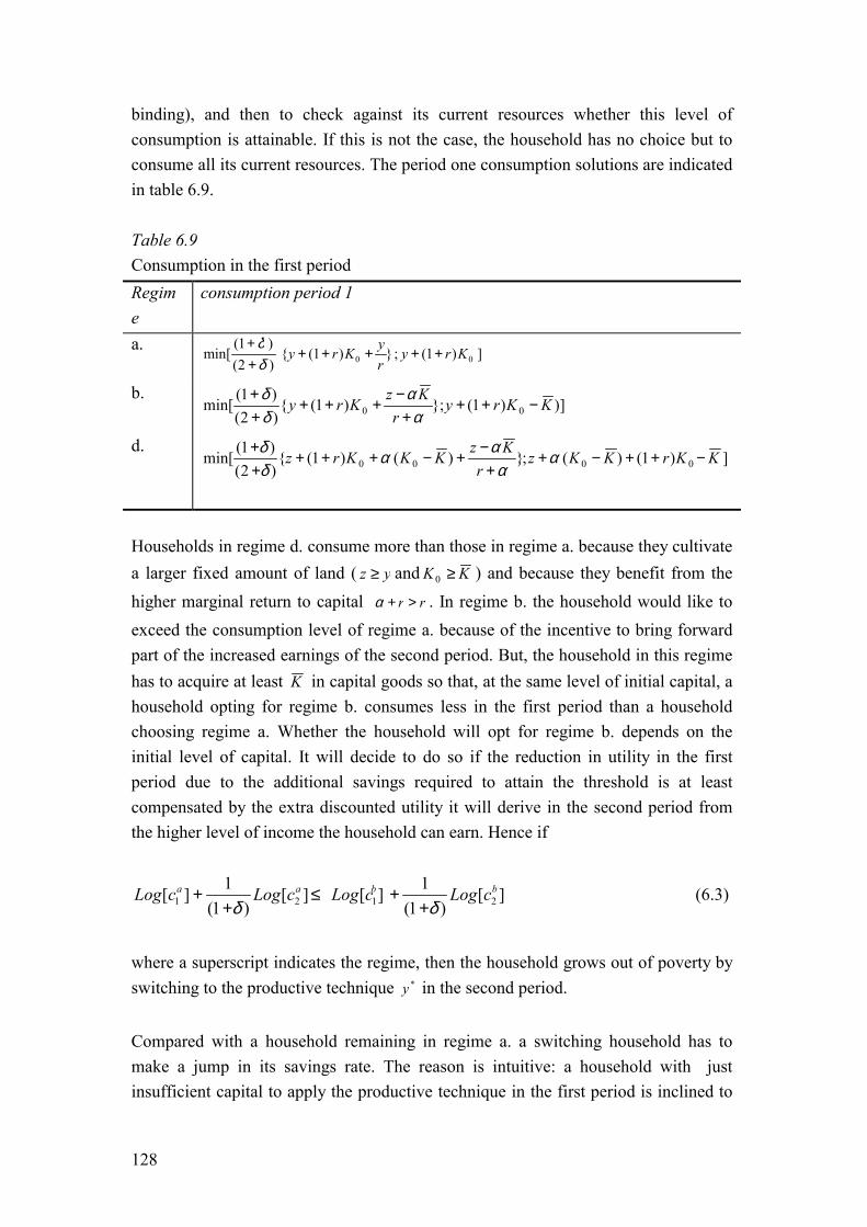
128

binding), and then to check against its current resources whether this level of consumption is attainable. If this is not the case, the household has no choice but to consume all its current resources. The period one consumption solutions are indicated in table 6.9. Table 6.9 Consumption in the first period Regime

consumption period 1

a. min[( )( )

{ ( ) }; ( ) ]12

1 10 0++

+ + + + +δδ

y r Kyr

y r K

b. ]))1(};)1({

)2()1(

min[ 00 KKryr

KzKry −++

+−

+++++

αα

δδ

d. ])1()(;})()1({

)2()1(

min[ 0000 KKrKKzr

KzKKKrz −++−+

+−

+−+++++ α

ααα

δδ

Households in regime d. consume more than those in regime a. because they cultivate a larger fixed amount of land ( yz ≥ and KK ≥0 ) and because they benefit from the higher marginal return to capital α + >r r . In regime b. the household would like to exceed the consumption level of regime a. because of the incentive to bring forward part of the increased earnings of the second period. But, the household in this regime has to acquire at least K in capital goods so that, at the same level of initial capital, a household opting for regime b. consumes less in the first period than a household choosing regime a. Whether the household will opt for regime b. depends on the initial level of capital. It will decide to do so if the reduction in utility in the first period due to the additional savings required to attain the threshold is at least compensated by the extra discounted utility it will derive in the second period from the higher level of income the household can earn. Hence if

][)1(

1][][)1(

1][ 2121bbaa cLogcLogcLogcLog

δδ ++≤

++ (6.3)

where a superscript indicates the regime, then the household grows out of poverty by switching to the productive technique y * in the second period. Compared with a household remaining in regime a. a switching household has to make a jump in its savings rate. The reason is intuitive: a household with just insufficient capital to apply the productive technique in the first period is inclined to

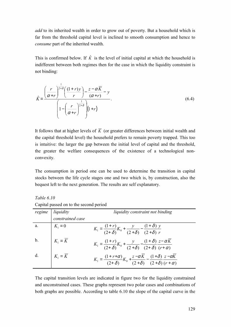
129

add to its inherited wealth in order to grow out of poverty. But a household which is far from the threshold capital level is inclined to smooth consumption and hence to consume part of the inherited wealth. This is confirmed below. If K� is the level of initial capital at which the household is indifferent between both regimes then for the case in which the liquidity constraint is not binding:

( )rr

r

yrKz

ryr

rr

K

+���

�

�

���

�

�

���

����

�

+−

−+

−−��

���

� +���

����

�

+=

+

+

11

)()1(

�2

1

21

δ

δ

α

αα

α. (6.4)

It follows that at higher levels of K (or greater differences between initial wealth and the capital threshold level) the household prefers to remain poverty trapped. This too is intuitive: the larger the gap between the initial level of capital and the threshold, the greater the welfare consequences of the existence of a technological non-convexity. The consumption in period one can be used to determine the transition in capital stocks between the life cycle stages one and two which is, by construction, also the bequest left to the next generation. The results are self explanatory. Table 6.10 Capital passed on to the second period regime liquidity

constrained case liquidity constraint not binding

a. 01 =K ryyKrK

)2()1(

)2()2()1(

01 δδ

δδ ++−

++

++=

b. KK =1 )()2(

)1()2()2(

)1(01 α

αδδ

δδ +−

++−

++

++=

rKzyKrK

d. KK =1 )()2(

)1()2()2(

)1(01 α

αδδ

δα

δα

+−

++−

+−+

+++=

rKzKzKrK

The capital transition levels are indicated in figure two for the liquidity constrained and unconstrained cases. These graphs represent two polar cases and combinations of both graphs are possible. According to table 6.10 the slope of the capital curve in the

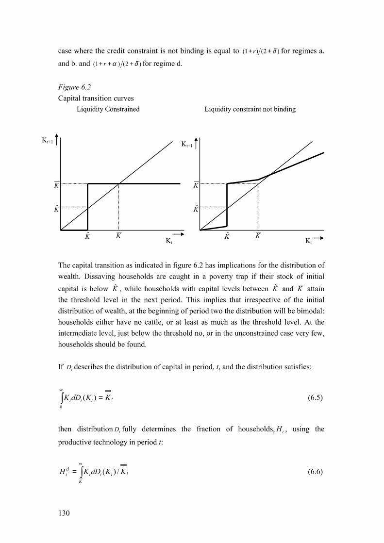
130

case where the credit constraint is not binding is equal to ( ) ( )1 2+ +r δ for regimes a. and b. and ( ) ( )1 2+ + +r α δ for regime d. Figure 6.2 Capital transition curves The capital transition as indicated in figure 6.2 has implications for the distribution of wealth. Dissaving households are caught in a poverty trap if their stock of initial capital is below K� , while households with capital levels between K� and K attain the threshold level in the next period. This implies that irrespective of the initial distribution of wealth, at the beginning of period two the distribution will be bimodal: households either have no cattle, or at least as much as the threshold level. At the intermediate level, just below the threshold no, or in the unconstrained case very few, households should be found. If Dt describes the distribution of capital in period, t, and the distribution satisfies:

tttt KKdDK =�∞

0

)( (6.5)

then distribution Dt fully determines the fraction of households, tH , using the

productive technology in period t:

t

Kttt

dt KKdDKH /)(�

∞

= (6.6)

Kt+1

Kt

Kt+1

Kt

Liquidity Constrained Liquidity constraint not binding

K

KK

K K�

K�

K�

K�

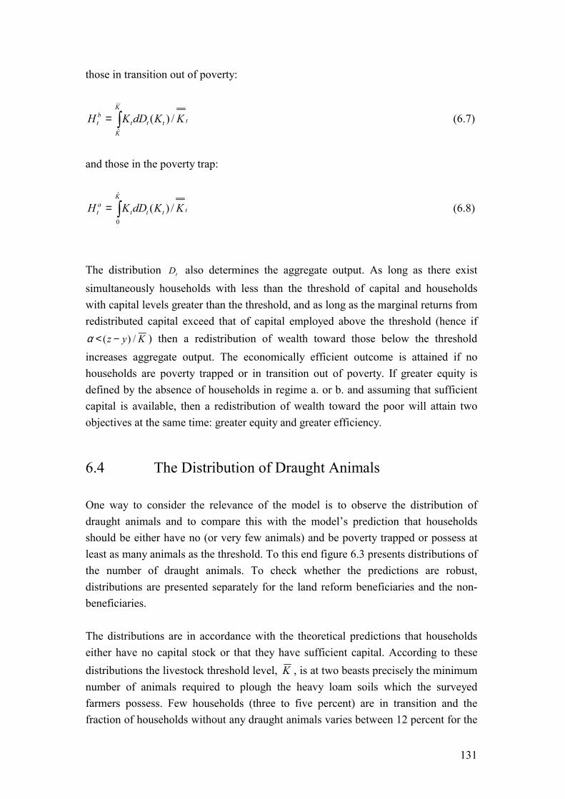
131

those in transition out of poverty:

t

K

Kttt

bt KKdDKH /)(

��= (6.7)

and those in the poverty trap:

t

K

tttat KKdDKH /)(

�

0�= (6.8)

The distribution Dt also determines the aggregate output. As long as there exist simultaneously households with less than the threshold of capital and households with capital levels greater than the threshold, and as long as the marginal returns from redistributed capital exceed that of capital employed above the threshold (hence if

Kyz /)( −<α ) then a redistribution of wealth toward those below the threshold increases aggregate output. The economically efficient outcome is attained if no households are poverty trapped or in transition out of poverty. If greater equity is defined by the absence of households in regime a. or b. and assuming that sufficient capital is available, then a redistribution of wealth toward the poor will attain two objectives at the same time: greater equity and greater efficiency.

6.4 The Distribution of Draught Animals One way to consider the relevance of the model is to observe the distribution of draught animals and to compare this with the model�s prediction that households should be either have no (or very few animals) and be poverty trapped or possess at least as many animals as the threshold. To this end figure 6.3 presents distributions of the number of draught animals. To check whether the predictions are robust, distributions are presented separately for the land reform beneficiaries and the non-beneficiaries. The distributions are in accordance with the theoretical predictions that households either have no capital stock or that they have sufficient capital. According to these distributions the livestock threshold level, K , is at two beasts precisely the minimum number of animals required to plough the heavy loam soils which the surveyed farmers possess. Few households (three to five percent) are in transition and the fraction of households without any draught animals varies between 12 percent for the

132

land reform beneficiaries and 26 percent for the communal households so that, again, the resettled households are found to be better off than the communal households. The wealth distributions presented do not originate from a unimodal normal or a lognormal distribution. Shapiro-Wilk tests, convincingly reject this possibility at above one percent levels of significance for each of the distributions presented. Figure 6.3 Histograms of the distribution of draught animals

Source: calculated using Kinsey�s surveys

Non-beneficiaries

0

0.05

0.1

0.15

0.2

0.25

0.3

1 2 3 4 5 6 7 8 9 10 11 12 13 14 15 16 17 18 19 20

number of draught animals

Land reform beneficiaries

0

0.02

0.04

0.06

0.08

0.1

0.12

1 2 3 4 5 6 7 8 9 10 11 12 13 14 15 16 17 18 19 20

number of draught animals

133

6.5 The Production Technology Another way to test the relevance of the model is to explore the dependence of the area cultivated on the availability of draught animals and to consider whether the non-convex production function depicted in figure 6.1 can be found. To this end a regression analysis is carried out. For the land reform beneficiaries, information pertaining to the seasons 1992-93 up to 1997-98 could be used, for the non-beneficiaries information for the seasons 1996/97 and 1997/98. Information for the first agricultural season available could not be included because of the timing of the surveys due to which information on livestock ownership and household composition are collected in different years (see chapter three). This leaves for the estimations six years of complete information for the land reform beneficiaries and two years of information for the communal households. Due to missing information 101 observations (out of a total of 2700) were dropped, 91 of which were land reform beneficiaries and 10 non-beneficiaries. In the estimation the total area, yi,t, cultivated is to be explained. The key explanatory variables Xi,t are the number of draught animals and the available family labour.

tititi Xy ,,, εβ += (6.9)

The estimated equation is linear. An obvious disadvantage of this approach, as opposed to a Cobb Douglas production function for instance, is that complete substitution between animal power and labour is allowed for, so that production can take place in the absence of labour. In the estimation this problem does not occur because there are no households without labour for the straightforward reason that if there are no persons in a household it seizes to exist. But land happens to be cultivated even when no draught animals are available. It is precisely this flexibility offered by the linear approach, which makes it the preferred choice. In accordance with the distribution of wealth shown in figure 6.3 a break is expected at two draught animals. To this end the model is estimated in piecewise linear form with a constant term included for households with at least one span of draught animals. In the figures presented in section 6.3, possessing a draught animal team was suggested to increase the area cultivated ( yz > ). The incorporation of the latter dummy is to check this assumption. Note however that the model does not depend on this assumption, as the relevant condition for z is: yz ≥ . As it is likely that there are diminishing returns to the use of draught animals, a squared term is included which is

134

expected to have a negative sign. In addition, to reflect that hiring draught services does take place (though on a limited scale), the monetary outlays spent on such services (in real 1990 Zimbabwe dollars) are included in the estimation. Because of the flow of events in time where planting precedes harvesting, reverse causality where planting a larger acreage leads to more livestock and labour bears little realism. But there may be concern of a potential bias in the parameter estimates due to omitted variables. For instance, it could be argued that agro-ecological factors or farming skills determine the acreage under cultivation. These factors are omitted from the regression, and therefore implicitly subsumed in the error term of the model. If these factors are significant determinants of the area cultivated, the error term will not converge to zero in the probability limit, and the parameters for the included explanatory variables will be inconsistent. Another variant of this problem would occur if some of the determinants themselves depend on omitted variables. For instance, the size of the labour force may depend on omitted farming skills, for instance if a successful farmer marries an additional wife or if he becomes host to a larger than average number of extended family members. Because the omitted factors are subsumed by the error term, these determinants are now correlated with the error term, and hence give rise to inconsistent parameter estimates. One solution to the potential problem of omitted variables is the use of a fixed effects model. Mundlak (1978) shows that the BLU estimator is the fixed effects within estimator for the case where all exogenous variables are not truly exogenous which is the case here. The estimated equation looks as follows:

tiiititi DXy ,,, εγβ ++= (6.10)

where Di is a household specific dummy and in which εi,t is the independent and identically distributed error term, Xi,t the vector of explanatory variables and yi,t the area under cultivation. The results reported in table 6.11 confirm for the land reform beneficiaries the non-convexity in the production technology and the existence of a threshold effect. All coefficients have the expected sign and the level of significance of each of the variables is within an acceptable range. For the communal households this is not the case. Except for the real cost of ploughing services all coefficients are insignificant.

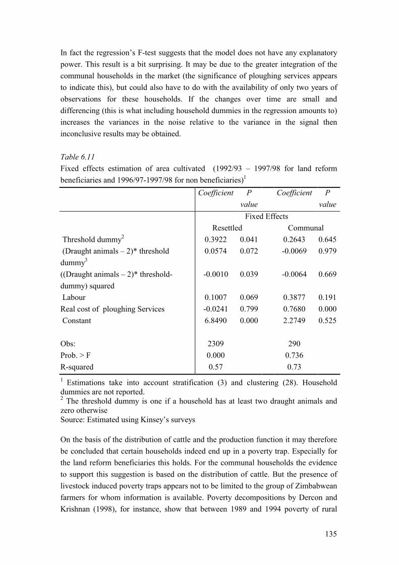
135

In fact the regression�s F-test suggests that the model does not have any explanatory power. This result is a bit surprising. It may be due to the greater integration of the communal households in the market (the significance of ploughing services appears to indicate this), but could also have to do with the availability of only two years of observations for these households. If the changes over time are small and differencing (this is what including household dummies in the regression amounts to) increases the variances in the noise relative to the variance in the signal then inconclusive results may be obtained. Table 6.11 Fixed effects estimation of area cultivated (1992/93 � 1997/98 for land reform beneficiaries and 1996/97-1997/98 for non beneficiaries)1

Coefficient P value

Coefficient P value

Fixed Effects Resettled Communal Threshold dummy2 0.3922 0.041 0.2643 0.645 (Draught animals � 2)* threshold dummy3

0.0574 0.072 -0.0069 0.979

((Draught animals � 2)* threshold-dummy) squared

-0.0010 0.039 -0.0064 0.669

Labour 0.1007 0.069 0.3877 0.191Real cost of ploughing Services -0.0241 0.799 0.7680 0.000 Constant 6.8490 0.000 2.2749 0.525 Obs: 2309 290 Prob. > F 0.000 0.736 R-squared 0.57 0.73

1 Estimations take into account stratification (3) and clustering (28). Household dummies are not reported. 2 The threshold dummy is one if a household has at least two draught animals and zero otherwise Source: Estimated using Kinsey�s surveys On the basis of the distribution of cattle and the production function it may therefore be concluded that certain households indeed end up in a poverty trap. Especially for the land reform beneficiaries this holds. For the communal households the evidence to support this suggestion is based on the distribution of cattle. But the presence of livestock induced poverty traps appears not to be limited to the group of Zimbabwean farmers for whom information is available. Poverty decompositions by Dercon and Krishnan (1998), for instance, show that between 1989 and 1994 poverty of rural

136

households in Ethiopia did not decline for those without oxen, while it significantly declined for households which own at least one oxen. Cavendish (1999) reports something similar. He finds a widening in the dispersion of the wealth distribution for communal farmers in Zimbabwe in the four years following the 1992 drought in which 80 percent of all cattle died. He explains this from the fact that for given land holdings, and in contrast to those whose draught animals survived, farmers who lost all cattle were unable to recover. Temporary shocks thus appear to create a more permanent distributional shift for the worse.

6.6 Conclusion

In this chapter the role of cattle in income generation has been considered. Cattle were shown to be an important productive asset and to obtain a good income from farming a team of oxen was shown to be required. Since households without traction animals earn a low income, and as these animals are expensive, it is suggested that once traction animals have been lost, it may be hard to obtain the resources to purchase new ones. Households facing such a situation could find themselves in a poverty trap. The possibility of a poverty trap for smallholder farmers who rely on animal traction for land preparation was derived in a theoretical model. This model was developed under strict conditions on the absence of credit and rental markets as this was believed to reflect the reality of smallholder agriculture in Zimbabwe. Galor and Zeira (1993) have shown however that under much weaker conditions similar results for the existence of a poverty trap can be attained. The model�s prediction on the existence of a bimodal distribution of wealth was confirmed for both the land reform beneficiaries and the non-beneficiaries. Evidence for the existence of a non-convex production technology was also found, but is solely for the land reform beneficiaries for whom more years of information was available and that better fit the description of a typical African farmer. The finding that cattle are important for income generation and that households may end in a poverty trap, in combination with the fact that households may lose their draught animals, because they had to be sold, died or were stolen, is reason to consider insurance arrangements that focus on cattle. Obviously such an arrangement would not help to smooth consumption directly, it would also help to smooth income. An additional advantage of such an arrangement is that if it is successful in avoiding poverty traps, it contributes to a more equitable distribution of wealth and a more efficient use of resources.

Bride Wealth as Informal Insurance

7.1 Introduction It follows from the importance of cattle for agricultural production and the existence of a livestock induced poverty trap that cattle may be considered a source of risk. Households losing their draught animals not only lose their prime asset for consumption smoothing they may even end up in a poverty trap. This raises the question whether there exist informal insurance arrangements that secure a household�s access to cattle. Such an arrangement would meet important welfare concerns by improving both the possibility to smooth income and to smooth consumption. After all, cattle are an important buffer stock as well. In this chapter it is suggested that Shona customary marriage (in which bride wealth is demanded in the form of cattle) can be interpreted as an informal security enhancing arrangement whose objective is to ensure a household�s access to cattle. The suggestion that unpaid bride wealth enhances household security is new. In the anthropological literature bride wealth payments are primarily identified as means to ascertain the continuation of the lineage or as compensation for loss of labour (Goody and Tambiah 1973; Holleman 1975; Kuper, 1982; Tambiah, 1989). Others stress the

138

ritual significance of bride wealth by showing how it binds families and their relations to the ancestors (SALC, 1997). In doing so it facilitates the pooling of resources (Rosenzweig, 1988; Rosenzweig and Stark, 1989; Baerends, 1991) or the diversification of income risk (Arnott and Stiglitz, 1991). The way bride wealth improves household security is not unlike the security offered by contingent credit arrangements described by Udry (1990 and 1994) for Northern Nigeria. These credit contracts comprise an insurance element because loan repayment depends on the economic condition of the agents involved. Creditors are lenient if their debtors go through a difficult period, while debtors make an extra attempt to repay if their creditor is in trouble. The marriage arrangement comprises similar elements. Instead of an outstanding loan, a claim is generated by demanding bride wealth for a daughter when she gets married. Only part of this is paid by the groom at the date of marriage. The bulk remains outstanding and its repayment is contingent on the economic situation of both the groom and his father in law. There are several important differences between the bride wealth arrangement of the Shona and Udry�s contingent credit suggestive of its importance as insurance. The size of the claims is of a different order of magnitude (two to five years of average household income). Next the duration for which claims remain outstanding is much longer; complete repayment often takes a lifetime. Additionally by associating claims to marriage, virtually nobody is excluded from the benefits of the arrangement. This is of importance, especially for the vulnerable who risk exclusion from informal insurance arrangements at times of covariate shocks (e.g. Sen, 1981). Associating claims to marriage also enhances enforcement possibilities for instance by threatening to take one�s daughter (and her children) back if the son in law fails to meet his bride wealth obligations. And finally by creating a network of affines connected through claims and liabilities, the bride wealth system manages to combine the advantages of a large risk pool with the benefits of close monitoring. The chapter is organised as follows. In section 7.2 it is shown how a claims and liabilities arrangement can enhance security, and that to do so the arrangement should be contingent and the size of the claim large. The following section contains the main assertion of this chapter. It is identified that the bride wealth arrangement of the Shona is a claims and liabilities arrangement and it is confirmed in an empirical test that the arrangement is conditional. In section 7.4 implications of the security enhancing interpretation of the bride wealth arrangement are considered. Consequences for contract enforcement, for use of the arrangement by those whose incomes are less subject to variability, for the use of the bride wealth arrangement and the timing of marriage by the poor, for efficiency and the existence of other

139

informal security enhancing arrangements are treated along with the question whether bride wealth as security enhancing mechanism is confined to Zimbabwe. Section 7.5 presents conclusions.

7.2 Conditional Claims and Liabilities The problems precluding the appearance formal insurance arrangements in rural Zimbabwe do not imply that informal insurance arrangements directed at idiosyncratic risks cannot be introduced. Especially in communities where the cost of information collection can be kept down, contract enforcement is facilitated by the interlinked nature of transactions, punishment of non-compliers is possible and premiums are collected after the event, informal insurance arrangements can flourish.55 One such possibility is an arrangement in which each household has the right to put a claim on another household (and an offsetting obligation to meet a request). A claims and liabilities arrangement may provide security if claims have to be honoured irrespectively of the wealth status of the requesting household. This kind of arrangement can be organised as follows.56 At its start a group of households issues claims on each other such that the net wealth position of each participant remains unchanged. After the issuance each household holds both a claim on a household in the pool and is indebted to another household in the same pool. If there are three households and the size of the debt is x then A holds a claim of x on B and has an obligation of similar size with respect to C. If B has a claim of x on C then each of the households in the pool is connected through claims and liabilities. If household A is the household in the illustration, then it may obtain the resources to purchase draught animals by effectuating its claim on B. If B cannot fulfil the request it may approach C and use the resources received to fulfil the obligation toward A. The passing on of the claim till it has reached a net provider of goods may be considered a way to deal with small risk pools by creating a string of bilateral relations. A � B � C

55 Without specifying which kind of informal arrangements exist at the community level, chapter four presented evidence in support of their existence.

56 This mechanism has also been described as a possibility in the theoretical literature (Gauthier, Poitevin and González, 1997), but only for the case where ex ante payments are made irrespective of the realization of risk. In this case, the transfer is conditional on the realization of the risk, but independent of the state of wealth of the household.

140

Obviously if C is not able to fulfil the request, it may approach A. In that case the arrangement fails because all claims and liabilities cancel. This could occur in the instance of a covariate shock. One way to avoid this is to ensure that the pool of households from which can be claimed is large, implying a long chain of individual relations. Another possibility is to broaden the claim to include all endowments, so that even in the event of an aggregate income shock, claims can be put on the buffer stocks of well endowed households. A third option is to allow claims to be unfulfilled for a prolonged period of time and to wait till the debtor has accumulated sufficient wealth to repay. This strategy obviously only works if there is sufficient change in wealth status over time. For a proper functioning of the arrangement the claims should not be too small. There are at least two reasons for this. First if claims and liabilities are created only once, they will have to do a lifetime. More importantly having considerable claims is instrumental in avoiding a situation known within an IS-LM framework as the monetarist model. The monetarist model describes a situation in which there is insufficient liquidity around causing the transactions need for money to become the limit on output. In our if case claims are too small people might become hesitant to call them in out of fear for running out of claims in the future. But if agents become hesitant to effectuate their claims, it means that they are not easily passed on from one household to the next. It follows that the means of dealing with small risks pools through a string of relations collapses and that the size of the risk pool becomes limited to those indebted to you. A sizeable claim helps to avoid this situation. Unlike in a credit transaction where credit is demanded ex post, one expects no interest to be paid in this ex ante arrangement. The reason for this is that a conditional claims and liabilities arrangement increases the net present value of expected utility of any participating household by reducing the variability of future income. Hence it is attractive to participate in a claims and liabilities pool, even in the absence of a possibility to demand interest. If a family is only prepared to join if interest is paid on net balances then other households would appear demanding less interest, effectively bidding the interest on the arrangement down to zero. But if a household used its claim but it did not yet fulfil its obligation then it is a net recipient of resources. In the absence of interest payments it follows that there is a real transfer of resources (unpaid interest) from the wealthy household to the poor one. This is a risk pooling element in the claims and liabilities arrangement. If the total outstanding claim is sufficiently large, then it may allow the household to deal with all idiosyncratic risk. In that case the claims and liabilities mechanism is an alternative for informal insurance (provided that in the long run all households earn

141

equal amounts). But if the total amount of claims is relatively small, then it pays to only effectuate these if the household needs them for instance when it is affected by grave events. And if it holds more than one claim, it will first effectuate the one on a relatively wealthy household so as to increase the probability of payment and to avoid a circular cancellation of claims and liabilities. This suggests that the arrangement automatically becomes conditional even if it was not intended to be so originally. There is an additional reason why one expects a claims and liabilities arrangement to be conditional. If a household would have to fulfil a claim when it does not possess the resources (including outstanding claims) to do so, then for precautionary reasons the household may decide not to participate in a claims and liabilities pool.57 A way to avoid refusal is to ensure that the obligation to repay debt is conditional on possessing sufficient resources (including outstanding claims).

7.3 Shona Marriage as Informal Insurance Mechanism Shona marriage is a family affair and its arrangement takes a substantial period of time during which the families involved have many opportunities to familiarise themselves.58 The choice of spouses is left to the individuals concerned but has to be sanctioned by their parents. If the families of the prospective partners agree with the choice of their children, negotiations involving senior representatives of each family start about the compensation required for the girl: the bride wealth. Bride wealth is divided into two portions of which roora is the more substantial part.59 It is a payment in cattle and cash and is associated with rights by the groom�s family over the children born from the union. Roora is paid to the father of the bride. He can do with it as he likes but preferably he reserves the cattle received for the marriage exchanges of the young men of his family as they are entitled to receive from their father the cattle required for their first marriage. Full payment of roora is extended over a prolonged period. After paying the first instalment of roora, the wife moves to the family of her husband where she is handed over to the head of the family of the groom. Only after a few days does he transfer the bride to her husband. In this way he underscores the family character of the marriage. After the girl has moved to the household of her husband the families remain related through a claim/liability, providing security to the girl�s family. Details of this arrangement are considered below. 57 See also Skinner (1988) for a similar argument as to why households facing fluctuating incomes may be hesitant to borrow.

58 Shona marriage is extensively described in Holleman (1975), Bourdillon (1987), Weinrich (1977), Kileff and Kileff (1992), Meekers (1993), Vijfhuizen (1998) and Dekker and Hoogeveen (2000).

142

7.3.1 Information Problems and Covariance of Risk Like formal insurance, informal insurance has to deal with information problems and problems posed by aggregate risk. To solve the former, detailed information on the incomes (and effort!) of the participants in the insurance pool is needed. If the members of the pool live in the same village, whether a farmer is hard working may be regarded to be common knowledge. Estimating each other�s income is also feasible. A well trained farmer should be able to reliably guess someone�s harvest from the crops observed in the field. Among the Shona even this skill is not required. Unlike in other places farmers are not secretive about their proceeds. After harvesting maize for instance (the main crop and staple food), the cobs are dried in stacks put up outside the household and observable by anyone. Information problems about the receipt of a household�s income therefore are not insurmountable obstacles for informal arrangements among the Shona. A more pressing issue for an insurance operating in rural areas with rain-fed farming, is the problem posed by aggregate risk. Income is closely related to the weather and as weather is strongly geographically correlated, pooling of household incomes can do little in terms of insurance. Consider table 7.1 for instance. It shows that crop and household income are highly correlated with national rainfall (correlation coefficients of 0.31 and 0.26 respectively). For insurance companies operating at the national level, these correlations might suggest scope for their services but for an informal arrangement such spreading is usually not attainable. Besides the problem caused by covariance is not entirely reflected in the correlation coefficients. In 1992 for instance, a drought year, two third of the households did not harvest any maize and the households that harvested something produced an output that was one fifth of the mean harvest produced between 1991 and 1998. In 1995 another drought hit the country which left a quarter of all households without any maize to harvest. The remaining households produced only half of the 1991-1998 average. A local insurance trying to cover these risks from insurance premiums would easily go bankrupt in these circumstances. A solution for this problem is not to pool incomes but to look for an insurance mechanism vested in a good that is less correlated with rainfall but which is still an important determinant of income. Livestock is an option here. As table 7.1 shows, household cattle ownership is only weakly (and insignificantly) correlated with

59 The first, called rutsambo, is usually an amount in cash or clothing. It is paid during he early stages if the bride wealth negotiations and is associated with the sexual rights in the woman.

143

national rainfall. But, as was argued in the previous chapter, the possession of cattle is closely associated with the ability to earn agricultural income. Table 7.1 Correlation coefficients for the period 1991/2-1997/81

National rainfall in mm

Household crop income 0.31 * Household real total income2 0.26 * Household maize yield 0.40 * Household cattle - 0.04 Real value of livestock sold - 0.17 *

1All income sources are in Z$1990. An asterix indicates a correlation significant at the 1 percent level or higher. 2 Total income comprises gross income from agriculture and own enterprises, income from livestock products, public transfers and private remittances and income from off farm employment. 3Measured in livestock equivalents, based on median prices. Source: Kinsey�s surveys. Rainfall data obtained from the Zimbabwean Meteorological Service. The marriage arrangement makes use of the independence of cattle ownership and rainfall as cattle represents the bulk of the value of roora demanded. In 1995 the most recent year for which marriage information was collected, of the 27 marriages concluded that year, bride wealth demanded consisted of Z$ 1765 in cash and 7.8 head of cattle. At a median value of cows, heifers and bulls of respectively Z$ 1200, Z$ 1000 and Z$ 1500 (table 3.7) it follows that approximately 85 percent of bride wealth is demanded in livestock units. If a livestock based insurance mechanism is to function, the information problem surrounding the ownership of livestock has to be solved. Fortunately in Zimbabwe it is not difficult to establish the number of cattle a household possesses as the animals are put into the family kraal every night where they are to be observed by anyone. To the degree that direct observation is not possible (for instance because some beasts have been lent) then the daughter/wife is in a unique position to ensure an impartial flow of information between the two families bond by a claim/liability arrangement, to which she is intimately connected. There are two additional arguments to base an insurance mechanism on livestock. First, cattle is the main store of wealth. Even if one does not intend to use the animals for ploughing, they are still useful as buffer stock to be liquidated in adverse

144

circumstances. Kinsey et al. (1998) show for instance that livestock sales were the primary source of money for food purchases during the 1992 and 1995 droughts in Zimbabwe. Table 7.1 (like figure 4.3) confirms this. It shows that the sale of cattle is strongly (negatively) correlated with rainfall. Second, households without sufficient draught animals risk to end in a poverty trap (chapter 6). So the possession of a minimum number of draught animals is a major concern. And as the number of cattle may be decimated by exogenous events (which can permanently affect a household�s wealth status), an insurance mechanism that ensures access to beasts in adverse circumstances has great value.

7.3.2 Outstanding Claims If the demand of bride wealth is to result in a claim with an insurance function three criteria have to be met. First, all bride wealth should not be paid at the time of marriage. Amongst the interviewed households there is clear resentment against those paying their bride wealth too quickly. Doing so is associated with the denial by the son in law of the relationship between his family and their in laws (Dekker and Hoogeveen, 2000). Second, given that weather risk is an annual phenomenon and that the total amount which can be claimed limited (when all daughters are married, additional claims cannot be generated), a payment schedule that lasts a long time, preferably a life time, is attractive. Thirdly, the claim has to be conditional. In this way one is able to obtain cattle when such is needed and one avoids having to provide cattle when animals cannot be spared. The first two issues are treated in this subsection. The third aspect is treated separately. 21 percent of the 571 married couples for which information is available, finished paying their bride wealth liabilities. In 79 percent of the marriages, cattle payments were still due. Figure 7.1 presents a kernel estimation of the number of livestock paid as function of the years of marriage. It shows that about ten percent is paid at the time of marriage. After 35 years of marriage about 20 percent of bride wealth is still outstanding. Both are in accordance with the insurance function of claims.

145

Figure 7.1 Kernel estimation of the percentage of bride wealth outstanding and the duration of the marriage

Source: estimated using Kinsey�s surveys That after 35 years a substantial part of bride wealth is still outstanding, does not imply that bride wealth is not paid in full. On the contrary, at the death of one of the spouses several options for the repayment of bride wealth may be explored. If the wife died young and she has unmarried sisters, one of them might replace her in a substitution marriage. If the husband died young, a brother might replace him in a replacement marriage. In each of these cases, the remaining liabilities are passed on to the new couple. If substitution or replacement marriages do not take place, the outstanding debt may be paid from the inheritance (resulting in an outtransfer of cattle). A relatively new phenomenon is that the wife of the deceased is allowed to remarry. In that case, the husband�s brother will take care of the widow, but allow other men to date (and marry) her. Any bride wealth received will then be used to repay outstanding bride wealth liabilities. If none of these options is available, the bride wealth liabilities are taken over by the family of the deceased groom.

7.3.3 Conditionality of the Arrangement For marriage claims to enhance security, it is essential for a family to provide bride wealth when it is relatively wealthy and to obtain bride wealth when in need If the household has to supply bride wealth when it is poor then the bride wealth system need not enhance household security and prudent families will be reluctant to participate because they run the risk to have to give up resources when they are already low.

.

pe

rce

nta

ge

pa

id

years of marriage0 10 20 30 40 50 60

0

.2

.4

.6

.8

1

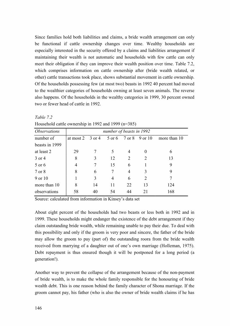
146

Since families hold both liabilities and claims, a bride wealth arrangement can only be functional if cattle ownership changes over time. Wealthy households are especially interested in the security offered by a claims and liabilities arrangement if maintaining their wealth is not automatic and households with few cattle can only meet their obligation if they can improve their wealth position over time. Table 7.2, which comprises information on cattle ownership after (bride wealth related, or other) cattle transactions took place, shows substantial movement in cattle ownership. Of the households possessing few (at most two) beasts in 1992 40 percent had moved to the wealthier categories of households owning at least seven animals. The reverse also happens. Of the households in the wealthy categories in 1999, 30 percent owned two or fewer head of cattle in 1992. Table 7.2 Household cattle ownership in 1992 and 1999 (n=385) Observations number of beasts in 1992 number of beasts in 1999

at most 2 3 or 4 5 or 6 7 or 8 9 or 10 more than 10

at least 2 29 7 5 4 0 6 3 or 4 8 3 12 2 2 13 5 or 6 4 7 15 6 1 9 7 or 8 8 6 7 4 3 9 9 or 10 1 3 4 6 2 7 more than 10 8 14 11 22 13 124 observations 58 40 54 44 21 168 Source: calculated from information in Kinsey�s data set About eight percent of the households had two beasts or less both in 1992 and in 1999. These households might endanger the existence of the debt arrangement if they claim outstanding bride wealth, while remaining unable to pay their due. To deal with this possibility and only if the groom is very poor and sincere, the father of the bride may allow the groom to pay (part of) the outstanding roora from the bride wealth received from marrying of a daughter out of one�s own marriage (Holleman, 1975). Debt repayment is thus ensured though it will be postponed for a long period (a generation!). Another way to prevent the collapse of the arrangement because of the non-payment of bride wealth, is to make the whole family responsible for the honouring of bride wealth debt. This is one reason behind the family character of Shona marriage. If the groom cannot pay, his father (who is also the owner of bride wealth claims if he has

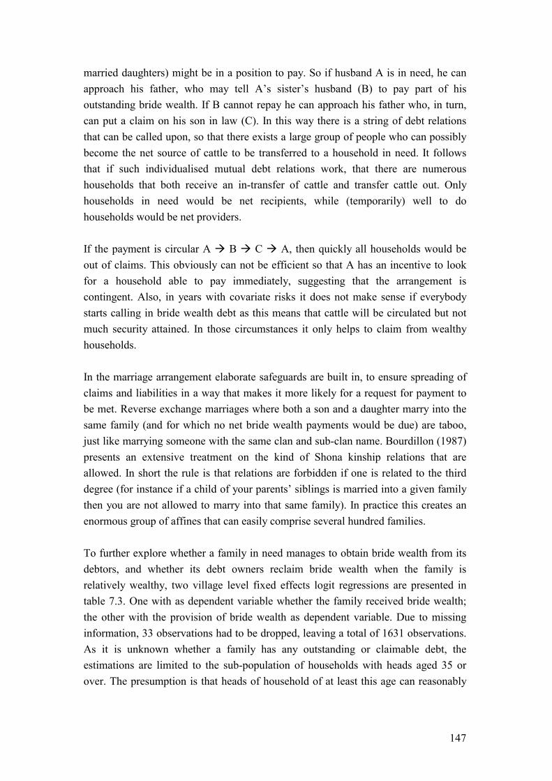
147

married daughters) might be in a position to pay. So if husband A is in need, he can approach his father, who may tell A�s sister�s husband (B) to pay part of his outstanding bride wealth. If B cannot repay he can approach his father who, in turn, can put a claim on his son in law (C). In this way there is a string of debt relations that can be called upon, so that there exists a large group of people who can possibly become the net source of cattle to be transferred to a household in need. It follows that if such individualised mutual debt relations work, that there are numerous households that both receive an in-transfer of cattle and transfer cattle out. Only households in need would be net recipients, while (temporarily) well to do households would be net providers. If the payment is circular A � B � C � A, then quickly all households would be out of claims. This obviously can not be efficient so that A has an incentive to look for a household able to pay immediately, suggesting that the arrangement is contingent. Also, in years with covariate risks it does not make sense if everybody starts calling in bride wealth debt as this means that cattle will be circulated but not much security attained. In those circumstances it only helps to claim from wealthy households. In the marriage arrangement elaborate safeguards are built in, to ensure spreading of claims and liabilities in a way that makes it more likely for a request for payment to be met. Reverse exchange marriages where both a son and a daughter marry into the same family (and for which no net bride wealth payments would be due) are taboo, just like marrying someone with the same clan and sub-clan name. Bourdillon (1987) presents an extensive treatment on the kind of Shona kinship relations that are allowed. In short the rule is that relations are forbidden if one is related to the third degree (for instance if a child of your parents� siblings is married into a given family then you are not allowed to marry into that same family). In practice this creates an enormous group of affines that can easily comprise several hundred families. To further explore whether a family in need manages to obtain bride wealth from its debtors, and whether its debt owners reclaim bride wealth when the family is relatively wealthy, two village level fixed effects logit regressions are presented in table 7.3. One with as dependent variable whether the family received bride wealth; the other with the provision of bride wealth as dependent variable. Due to missing information, 33 observations had to be dropped, leaving a total of 1631 observations. As it is unknown whether a family has any outstanding or claimable debt, the estimations are limited to the sub-population of households with heads aged 35 or over. The presumption is that heads of household of at least this age can reasonably

148

be expected to participate in the bride wealth system. In doing so the sample size was reduced to 1543 observations. The amount of livestock resources (before transfers) is taken as indicator of family wealth because Zimbabwean families associate livestock ownership strongly with wealth (Scoones, 1995). This should come as no surprise, given the important role draught animals fulfil in income generation and its role as buffer stock. Seen in this light, livestock ownership is probably a better proxy for a family�s permanent wealth status than household income which fluctuates strongly from year to year. Nonetheless, the latter factor is also included (as the log of real total household income) to inform on how resource fluctuations affect the transfer of bride wealth. Additionally, to capture the covariate element of income, rainfall in millimetres and measured at the national level is incorporated. For families providing and receiving bride wealth in a given year the order of events is not known, so that no causal inferences can be made. For our purposes this is fine as it does not matter whether a family first provided bride wealth, then considered its possession of wealth too low after which it called in bride wealth; or whether the family first received bride wealth and thereafter became more willing (and able) to honour a request for the repayment of outstanding debt. It is expected that it matters whether a household possesses sufficient draught animals for ploughing. Therefore a distinction is made between households that transfer bride wealth and possess a minimum number of draught animals and those that do not. The cut off point is put at 2.5 trained oxen equivalents, a number that allows the household to pull a plough. To allow for the fact that a household obtains a transfer of cattle as first instalment of bride wealth payment when a daughter gets married, a dummy variable is included for daughters aged 15 or over who got married and started to live with their husband. No information on marital status was available for those below the age of 15. A household may also experience an out-transfer of wealth following a death in the family. This will be the case if the deceased is a wife for whom bride wealth is still outstanding, but also if it is a husband who still has to pay part of the outstanding bride wealth. In either case one expects an out-transfer. This is included by a dummy variable for death in the family. Finally, differences due to participation in the land reform program are allowed for. To this end a dummy for non-beneficiary households is included.

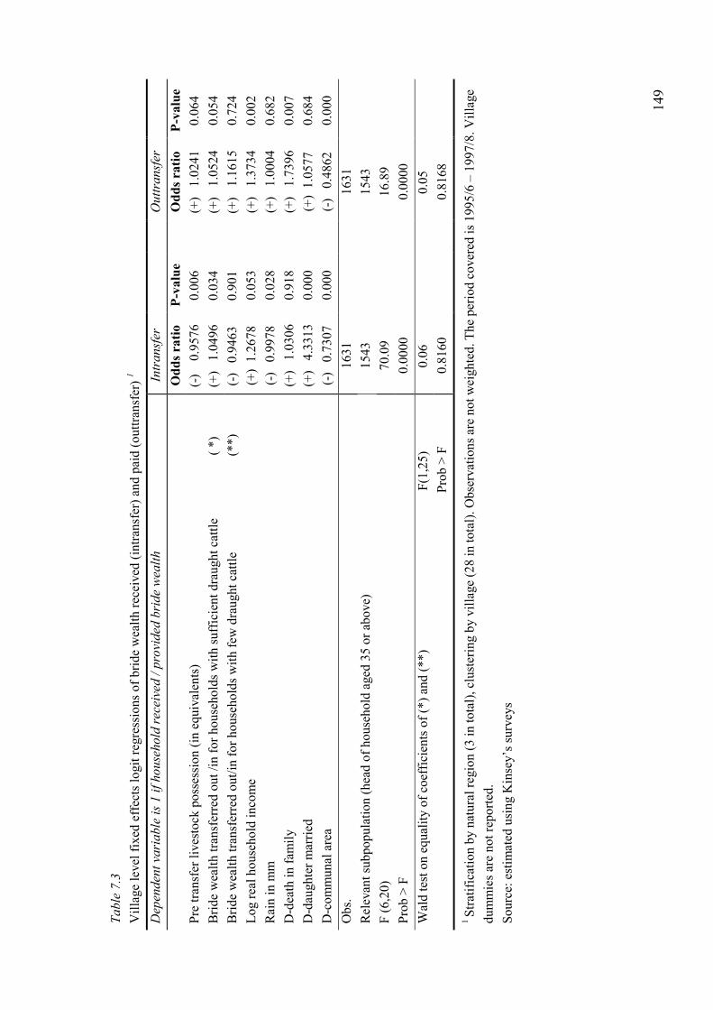
14

9

Tabl

e 7.

3 V

illag

e le

vel f

ixed

eff

ects

logi

t reg

ress

ions

of b

ride

wea

lth re

ceiv

ed (i

ntra

nsfe

r) a

nd p

aid

(out

trans

fer)

1 D

epen

dent

var

iabl

e is

1 if

hou

seho

ld re

ceiv

ed /

prov

ided

bri

de w

ealth

In

tran

sfer

O

uttr

ansf

er

Odd

s rat

io

P-va

lue

O

dds r

atio

P-

valu

e Pr

e tra

nsfe

r liv

esto

ck p

osse

ssio

n (in

equ

ival

ents

) (-)

0

.957

6 0.

006

(+

) 1

.024

1 0.

064

Brid

e w

ealth

tran

sfer

red

out /

in fo

r hou

seho

lds w

ith su

ffic

ient

dra

ught

cat

tle

(

*)

(+)

1.0

496

0.03

4

(+)

1.0

524

0.05

4 B

ride

wea

lth tr

ansf

erre

d ou

t/in

for h

ouse

hold

s with

few

dra

ught

cat

tle

(**

) (-)

0.

9463

0.

901

(+

) 1

.161

5 0.

724

Log

real

hou

seho

ld in

com

e (+

) 1.

2678

0.

053

(+

) 1

.373

4 0.

002

Rai

n in

mm

(-)

0.

9978

0.

028

(+

) 1

.000

4 0.

682

D-d

eath

in fa

mily

(+

) 1

.030

6 0.

918

(+

) 1

.739

6 0.

007

D-d

augh

ter m

arrie

d (+

) 4

.331

3 0.

000

(+

) 1.

0577

0.

684

D-c

omm

unal

are

a (-)

0.

7307

0.

000

(-)

0.

4862

0.

000

Obs

. 16

31

1631

Rel

evan

t sub

popu

latio

n (h

ead

of h

ouse

hold

age

d 35

or a

bove

) 15

43

1543

F (6

,20)

70

.09

16.8

9

Prob

> F

0.

0000

0.

0000

Wal

d te

st o

n eq

ualit

y of

coe

ffic

ient

s of (

*) a

nd (*

*)

F(

1,25

) 0.

06

0.05

P

rob

> F

0.81

60

0.81

68

1 St

ratif

icat

ion

by n

atur

al re

gion

(3 in

tota

l), c

lust

erin

g by

vill

age

(28

in to

tal).

Obs

erva

tions

are

not

wei

ghte

d. T

he p

erio

d co

vere

d is

199

5/6

� 19

97/8

. Vill

age

dum

mie

s are

not

repo

rted.

So

urce

: est

imat

ed u

sing

Kin

sey�

s sur

veys

150

The estimation results are reported in table 7.3. The first thing to note is the switching of the sign of the coefficient on pre-transfer livestock possessions. It is negative for receipt of bride wealth (implying that poorer households are more likely to obtain bride wealth) and positive for provision of livestock so that wealthier households are more likely to provide bride wealth. For households possessing sufficient draught animals, in-transfers of bride wealth are positively associated with out-transfers. The same holds for out-transfers of bride wealth which are positively associated with in-transfers. This suggests the circulation of cattle, a phenomenon reported by Mair (1977: 58) to be the �essence of the bride wealth system�. From our perspective it is a way to deal with the problem of small risk pools. Households receiving an in-transfer of bride wealth that are poor do not participate in the passing on of bride wealth: in their case the coefficient is insignificant. A Wald test (reported at the bottom of the table) shows that the coefficients for wealthy households differ significantly from those for poor households. It follows that wealthier households are the ones participating in the circulation of cattle, and not the poorer ones. In combination with the fact that the livestock poor are more likely to receive bride wealth and less likely to provide it, it suggests that cattle is circulated through society till it reaches its destination at a poor household. The more active involvement in the circulation of cattle of wealthy households, is also illustrated by the fact that those with higher incomes participate more actively in the provision and in the receipt of bride wealth: in both regression the signs for real income are positive. Despite this active participation by the wealthy, the bride wealth system is not immune to the consequences of covariate events. The regression for the in-transfer of bride wealth shows this: households are more likely to receive bride wealth in years of good rainfall. Death in the family leads to an out-transfer of bride wealth, either to settle unpaid bride wealth (in case a wife dies) or to deal with inheritance issues (in the case a husband dies). Marriage leads to an in-transfer in accordance with the results of the kernel regression presented as figure 7.1. Non-land reform beneficiaries participate less in bride wealth exchanges. This might be because resettled households, who started off as complete strangers, actively build networks within their own villages. One of the ways to do so is through intra-village marriages, which in turn, facilitates monitoring and the transfer of bride wealth. In communal areas intra-village marriages are uncommon. Another reason might be that land reform beneficiaries rely for a much larger fraction of their income on agriculture (in 1997/98 for instance crop income alone made out 64 percent of the income of land reform beneficiaries 40

151

percent of non-beneficiaries) thus making them more susceptible to livestock induced poverty traps and reliant on bride wealth transfer. In conclusion, the regressions confirm that unpaid bride wealth is a conditional arrangement allowing poor households to obtain resources. The probability of providing bride wealth increases with the possession of household wealth as measured in livestock equivalents. Households with higher incomes, and resettled households participate more actively in the bride wealth system. The arrangement is not immune to covariate risks and in years with little rainfall the probability to receive an in-transfer of bride wealth decreases.

7.4 Implications of the Insurance Interpretation of Bride Wealth

In the previous section the main result of this chapter was established: bride wealth claims and liabilities enhance household security by creating claims whose repayment is contingent on the economic situation of both the groom and his father in law. But the results of table 7.3 could be given a different interpretation if being wealthy is associated with having larger bride wealth liabilities. For instance if in the negotiations on the height of the bride wealth, the wealth of the father in law is taken into account in such a way that wealthier families demand less for their daughters than they have to pay for their sons. Or it could occur if households with a surplus of sons become relatively wealthy, because young men are more productive than young women. Unfortunately, household wealth at the time when bride wealth is demanded, and the total claims and liabilities of each household have not been recorded, so that this interpretation cannot be put to empirical scrutiny.60 Instead the insurance interpretation of marriage and several of its implications are considered in greater detain in this section.

7.4.1 Enforcement In section 7.2, it was stated that a �claims and liabilities arrangement may provide security if claims have to be honoured irrespectively of the wealth status of the requesting household�. How honouring claims can be assured has not been made

60 Since rainfall is the most important determinant of income in rural Zimbabwe, and as income and wealth are associated one way to check whether bride wealth depends on household wealth is to investigate the correlation between rainfall and bride wealth demanded. In regressions in which the amount of the bride wealth is explained by rainfall and in combination with a squared term, none turned out be significant.

152

clear, but obviously it is of interest to know how enforcement issues are solved in the bride wealth arrangement. That it is solved follows implicitly from the fact that bride wealth resources are transferred in a way that enhances household security. There are several mechanisms that improve the possibilities for contract enforcement. First there is the moral obligation that one has to pay its due, especially since bride wealth claims are generated before the event. So unlike a credit provider who may refuse to provide his personal resources to another household, someone who owes unpaid bride wealth is likely to feel obliged to fulfil a request for repayment. This is reinforced by the fact that he has received something important from the claimant: his wife. She, by the way is likely to make precisely this point to her husband. Secondly there is flexibility in the repayment. The number of cattle is carefully stipulated in the bride wealth negotiations, there is flexibility in the kind of beasts that have to be provided (Dekker and Hoogeveen, 2000). Finally there are the (extra) legal means of contract enforcement. In the marriage arrangement punishment may be imposed if the son in law is in a position to repay but refuses to do so. The claimant has the possibility to take his daughter and her children into custody until the demand for debt repayment, or a sufficient part thereof, is honoured (Holleman, 1975). The possibility to take one�s daughter and her children back, is a serious threat for two reasons. Firstly it deprives the unwilling husband of his contribution to the lineage and of sons that will take care of him in old age (Bourdillon, 1987). Secondly, in a society where labour markets are absent, family labour goes at a premium and ambitious men try to build around themselves a sizeable family of agricultural labourers (Binswanger and McIntire, 1987; Bourdillon, 1987). In many instances it is not necessary to resort to the drastic measures of custody and does it suffice to suggest that ancestors with the ability to cause barrenness in the marriage might be displeased by the refusal of the son in law. Such a threat is taken very seriously also because certain ceremonies in the marriage procedure, like the transfer of a cow to the mother of the bride (because she carried the daughter in her womb) which is subsequently dedicated to maternal ancestors, create a close connection between the payment of bride wealth and the birth of offspring (Holleman, 1975). Another possibility is to turn to a traditional court. The marriage procedure comprises several elements which facilitate ruling by traditional courts. Use is made of an intermediary for instance. This is a carefully selected, trustworthy person, who operates as go-between when the intention of marriage is made known to the family of the bride. He (women do not act as intermediary) acts as official witness to all marriage transactions and is expected to be an impartial observer. In court the intermediary is the official witness who reports in how far and in which manner the

153

parties have met their respective liabilities under the marriage agreement. Also the exchange of tokens (which in a society where illiteracy is common, have the status of written agreements) between the bride and her future husband at the initial stages of the marriage procedure facilitates court rulings (Bourdillon, 1987). If the court decides that cattle should be paid and the son in law perseveres in his refusal then the court has the power to confiscate the cattle required. These measures help to ensure the insurance function in the bride wealth arrangement. But in some instances this does not suffice. Approximately four percent of the marriages are dissolved on grounds that are related to the (non)-payment of bride wealth. These divorces are personal tragedies but they do not threaten the existence of the bride wealth insurance system. A divorced woman may remarry, in which case the bride wealth demanded will be lowered, dependent on the number of children she has given birth to (Dekker and Hoogeveen, 2000). Another way to opt out of the insurance arrangement is to fulfil a bride wealth obligation as soon as one is able to do so. But there is a social stigma preventing sons in law from doing so (Dekker and Hoogeveen, 2000). This stigma is still in place as is illustrated by the fact that bride wealth is repaid slowly over time. Of the 571 marriages only 21 percent had repaid all bride wealth cattle even though households possess sufficient cattle to do so. In fact in 30 percent of the cases, the head of household could repay the outstanding bride wealth liabilities of all married women residing in his household and still be left with at least six head of cattle!

7.4.2 Changes in Risk Voluntary informal insurance mechanisms may fail if households become more involved in the market economy or following the implementation of social safety nets like food for work schemes (Platteau, 1987; Dercon, 1999). The reason for this is opposite to the reason why punishment helps enforce an informal insurance arrangement. In this case the innovations provide extra possibilities for income smoothing. Since the informal insurance is voluntary, these additional possibilities undermine the functioning of the insurance by making opting out more attractive. Changes in Zimbabwe�s economic environment, which in turn affected the income variability of households, have indeed affected the marriage arrangement. Service marriages, at which the son-in-law works for the father of the bride to fulfil his bride wealth liabilities disappeared after the occurrence of a labour market (Holleman, 1975). More recently opposition has arisen against the passing on of wives in replacement marriages. Nowadays it is more common to allow them to remarry. This

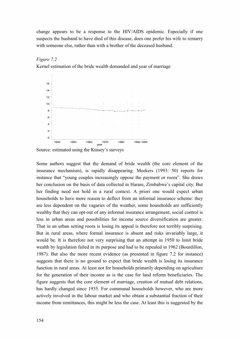
154

change appears to be a response to the HIV/AIDS epidemic. Especially if one suspects the husband to have died of this disease, does one prefer his wife to remarry with someone else, rather than with a brother of the deceased husband. Figure 7.2 Kernel estimation of the bride wealth demanded and year of marriage Source: estimated using the Kinsey�s surveys Some authors suggest that the demand of bride wealth (the core element of the insurance mechanism), is rapidly disappearing. Meekers (1993: 50) reports for instance that �young couples increasingly oppose the payment or roora�. She draws her conclusion on the basis of data collected in Harare, Zimbabwe�s capital city. But her finding need not hold in a rural context. A priori one would expect urban households to have more reason to deflect from an informal insurance scheme: they are less dependent on the vagaries of the weather, some households are sufficiently wealthy that they can opt-out of any informal insurance arrangement, social control is less in urban areas and possibilities for income source diversification are greater. That in an urban setting roora is losing its appeal is therefore not terribly surprising. But in rural areas, where formal insurance is absent and risks invariably large, it would be. It is therefore not very surprising that an attempt in 1950 to limit bride wealth by legislation failed in its purpose and had to be repealed in 1962 (Bourdillon, 1987). But also the more recent evidence (as presented in figure 7.2 for instance) suggests that there is no ground to expect that bride wealth is losing its insurance function in rural areas. At least not for households primarily depending on agriculture for the generation of their income as is the case for land reform beneficiaries. The figure suggests that the core element of marriage, creation of mutual debt relations, has hardly changed since 1935. For communal households however, who are more actively involved in the labour market and who obtain a substantial fraction of their income from remittances, this might be less the case. At least this is suggested by the

.

year1940 1950 1960 1970 1980 1990 1995

0

2

4

6

8

10

12

14

16

155

regression result that bride wealth exchanges are less actively explored by communal households.

7.4.3 Exclusion of the Poor Despite the existence of enforcement possibilities the poor might still be excluded from the security offered by the marriage arrangement. After all wealthy households have an incentive to collude against the poor (see chapter two). In chapter five, evidence of differences in the level of informal insurance between the poor and non-poor was not found. But does this also hold for the marriage arrangement? A priori the exclusion of the poor seems unlikely. No indications suggesting that children from poor families have difficulty to get married were found in the literature, nor was this issue raised in discussions with farmers. To explore this issue further, table 7.4 presents a mean comparison test on the fraction of poor and non-poor households that married a daughter. Following the findings of chapter six, where poverty was associated with the inability to plough, being poor is defined by possessing, in the year previous to the marriage, insufficient draught animals (or the livestock equivalent that would allow to purchase a set of draught animals) to plough. The test finds no evidence in support of exclusion of the poor from creating bride wealth claims: the fractions of daughters that marry do not differ statistically for poor and non-poor households. Table 7.4 Mean comparison test of fraction of poor and non-poor households marrying a daughter between 1994 and 1998 Fraction of

households Std. error

Obs.

Non-poor 0.098 0.01 1513 Poor 0.083 0.01 362 H0: mean (non-poor) � mean(poor) = x = 0 Ha: x < 0 x unequal 0 x > 0 T-stat 0.91 0.91 0.91 P-value 0.82 0.36 0.18

* T-test on the equality of means. Data are not assumed to have equal variances. Poor is defined as having less than or equal to 2.5 livestock equivalents in the year previous to the marriage. Marriages could only be determined for surveys held between 1995 and 1999. Resettled households only. Source: calculated using Kinsey�s surveys

156

Changing the perspective slightly, one expects the timing of marriage of unmarried daughters to be such that it coincides with a time when (i) cattle is desperately needed or (ii) when the household is in the �danger zone� so that it is good to have a debtor on which claims can be put. This possibility is explicitly recognised in what has been labelled credit marriages, the arrangement where a young daughter, in exceptional cases even a yet unborn girl, is promised for marriage in order to obtain advance payment of the bride wealth. Credit marriages are officially prohibited. Nonetheless Vijfhuizen (1998: 21) reports a surge in credit marriages after the 1992 drought in Chipinge District. Indeed daughters of poor households marry when they are relatively younger. This is suggested by the information presented in table 7.5 where it is tested whether the mean age of marriage is lower for girls from families with few head of cattle (labelled poor) relative to those with sufficient draught animals, the non-poor. Table 7.5 Mean comparison test of age at marriage of own daughters married between 1994 and 1998 from poor and non-poor households* Age at marriage Std.

error Obs.

Non-poor 21.9 0.34 170 Poor 20.6 0.59 40 H0: mean (non-poor) � mean(poor) = x = 0 Ha: x < 0 x unequal 0 x > 0 T-stat 1.93 1.93 1.93 P-value 0.97 0.06 0.03

* T-test on the equality of means. Data are not assumed to have equal variances. Poor is defined as having less than or equal to 2.5 livestock equivalents in the year previous to the marriage. Age at marriage could only be determined for surveys done between 1995-1999, reflecting the years 1994-1998. Resettled households only. Source: calculated using Kinsey�s surveys This finding supports (or at least it does not contradict) that the optimal timing of marriage over the household lifecycle would be to marry daughters early in life, and sons late. If daughters marry when they are young, then the household becomes a net claimant to unpaid bride wealth. If, during this period some bride wealth is repaid, this allows the household to experience a period of high returns. Late marriage of sons has several advantages: the loss of productive draught power for the first instalment of the bride wealth is postponed and, by postponing the marriage, the household has more time to accumulate sufficient cattle. If the household acquires many beasts, additional cattle becomes less productive so that the marriage of a son is relatively cheap in livestock terms. Unfortunately the available data do not allow us

157

to test whether the payment of bride wealth is a factor explaining the finding that Zimbabwean men enter their first marriage at a much later age than Zimbabwean women (Zimbabwe, 1995).61

7.4.4 Efficiency It was suggested in section 7.2 that in a conditional claims and liabilities arrangement no interest would be demanded of a household that is a net debtor. This reflects the risk pooling element in the bride wealth system. Only a household in need calls in (part of) its outstanding debt. In doing so it is likely to be due more than it owes. As a detailed assessment of livestock value in Zimbabwe�s communal areas by Scoones (1992) demonstrates that cattle yield a high return, this amounts to a substantial transfer of resources (unpaid interest). These high returns might be a reason to quickly call in all outstanding debt. After all, a family that ensures that its son-in-laws pay all bride wealth due and that is slow in paying its bride wealth liabilities, generates a high return from its action. That this does not happen (most bride wealth remains unpaid for a substantial period) illustrates that households value the option value of a livestock claim or that interest is paid. The latter is not the case. Only when repayment is urgently needed and the debtor unable to fulfil the request, will he try to give the impatient father in law a small contribution, which is not considered repayment of the outstanding bride wealth. And even this is considered to be more a sign of �the earnest inclination to pay off the debt� (Holleman, 1975: 173) than payment of interest. The absence of the demand of interest and the conditional receipt/payment of claims are the risk pooling elements in the bride wealth system. Obviously, these kinds of risk pooling are not fully efficient. A formal insurance would allow families to pool risks beyond unpaid interest on transferred endowments, and a formal credit agency would be able to offer credit beyond the limits imposed by the amount of outstanding bride wealth debt. Nevertheless, it is tempting to conclude that the presence of a security enhancing institution like Shona marriage implies a welfare gain relative to the situation where it would be absent: why else would this kind of arrangement have come into existence? But this interpretation need not hold in a dynamic context since the combination of marriage and bride wealth provides a link between procreation and security and puts a premium on having children (unmarried daughters). This is not inefficient per se, as long as the consequences of such an arrangement are fully borne by the household. But, the increase in the rate of birth is likely to have

61 The median age at first marriage for men is 25 years, compared with 19 for women. Only 11 percent of men are married by age 20, compared to 62 percent for women

158

spillover effects to other households. These might be negative, for instance when land becomes scarce, or positive when increased population pressure leads to technological innovations. An additional aspect is that it is unclear what the consequences of the bride wealth arrangement are for other informal insurance mechanisms. The need for such arrangements has diminished substantially as the size of the bride wealth claims and liabilities is large relative to income. At an average value of 7.8 head of cattle and Z$ 1765 in cash (in 1995) bride wealth represents two yearly incomes for resettled households and five for communal households! If one takes into account that in Zimbabwe a women at the end of her fertility would have given birth to 6.3 children (Zimbabwe, 1995), not all of whom survive or get married, then it suggests that households hold claims and liabilities representing a large part --25 percent is a conservative estimate, of their lifetime income. So the bride wealth system will negatively affect the incentive to join a different arrangement: a household holding claims and liabilities is already able to smooth away the worst fluctuations in income. Nevertheless, despite the existence of a bride wealth mechanism it was found in chapter four that the variability in household consumption is high. The need for additional insurance therefore remains. A conditional claims and liabilities mechanism could however also reinforce the functioning of informal insurance arrangements. This would be the case when the household is demanded to fulfil its bride wealth obligation at a time when it has to make a large net transfer to the pool. If the household has to fulfil this request first, then the net contribution to the pool diminishes and opting out of the insurance becomes less attractive. In any event, unambiguous conclusions about the Pareto improving character of Shona marriage or about the effects of the arrangement on the existence of other informal insurance mechanisms cannot be drawn.

7.4.5 Relevance beyond Zimbabwe This chapter has shown that the demand of bride wealth improves security for Shona households in Zimbabwe by associating marriage with the possibility to obtain livestock. Through its association with marriage, the enforcement problem is reduced because punishment which affects the procreation of the lineage is considered a serious threat. And by demanding livestock, the problems associated with covariate risks can be largely circumvented. The Shona are not the only ethnic group in Southern Africa that demand bride wealth and attribute a central role to cattle in their economy. The Xhosa, Twana, Zulu, Swazi, Ndebele, Khoi, Herero, San, Shona, Tonga, Lunda, Lozi, Ndemby, in short all but one of the ethnic groups living in southern Africa distinguished by Middleton et al. (1995) do so, just like the Nuer

159

who live in Sudan, the Gusii in Tanzania and the Turkana in Kenya. The only exception in Southern Africa are the Bemba, who live in a tsetse infested area and cannot keep cattle. The demand of bride wealth and the importance of cattle is not the only aspect uniting these ethnic groups. They also practice rain-fed agriculture in semi-arid tropical areas that can be characterised by land abundance and relatively low population density. These factors can in turn be associated with the absence of land, labour, formal credit and insurance markets and large geographically correlated weather risks (Binswanger en McIntire, 1987). The absence of labour markets creates a premium on family labour so that, like in Zimbabwe, enforcement of any informal insurance arrangement might be facilitated if it allows to pose a threat on the ability for procreation and the availability of family labour. Given that these ethnic groups face similar weather risk, use a comparable, draught power based, production technology and demand bride wealth in the form of cattle there is a fair reason to assume that they too make use of the possibility not to pay all bride wealth at the time of marriage. If they do so they enhance, the land reform beneficiaries, household security by creating claims and liabilities.

7.5 Conclusion In this chapter the marriage arrangement in Zimbabwe in which bride wealth is demanded for an unmarried daughter, is claimed to be an informal security enhancing mechanism. By providing households access to cattle the arrangement allows to prevent income shocks associated with the absence of draught animals. And because cattle are an important buffer stock, beasts obtained through the arrangement may also used for consumption smoothing purposes. To be functional as insurance mechanism, the arrangement has to deal with information problems and covariate risk. By expressing bride wealth primarily in cattle, information problems are dealt with because the number of cattle possessed can be observed by anyone. The importance of covariate risk is reduced because cattle ownership is much less correlated with rainfall than is income, while the ownership of cattle is closely associated with the ability to generate income. The claim of this chapter is supported by empirical evidence. Only a small fraction of bride wealth is shown to be paid at the time of marriage and most remains outstanding for a prolonged period. In regression analysis it is shown that bride wealth claims are contingent: families obtain resources when they are less well off while resources are provided by households that possess sufficient head of cattle.

160

The importance of the bride wealth as informal insurance arrangement stems from several factors. First, the amounts involved are large. The average value represented by unmarried sons and daughters is conservatively put at 25 percent of lifetime household income. Secondly, the mechanism incorporates nearly the complete adult population including the vulnerable who are most at risk of exclusion from informal insurance arrangements. And finally it is a smart way of creating a large insurance pool without the need for a central organisation that monitors each participant in the pool. To put the insurance interpretation of marriage to further scrutiny several of its implications are considered. It is shown how the arrangement is enforced by relying on different kinds of (threats with) punishment. The association of the arrangement with marriage facilitates enforcement as it creates possibilities for retribution. It is also shown that in urban areas, where income risks are smaller and diversification easier, opposition to bride wealth has arisen. This does not hold for rural households that depend for the generation of their income upon agriculture. No differences exist between poor and non-poor households in the fraction of daughters getting married, suggesting that poor households experience no greater difficulty in creating bride wealth claims as do others. But, daughters from households that are vulnerable to income shocks (the poor) and who therefore have a greater incentive to possess a positive balance in bride wealth claims marry younger. Sometimes poor households even promise their under-aged daughters into marriage. Though the insurance interpretation of marriage suggests that the arrangement enhances welfare it is shown that this need not be the case. The marriage arrangement may be an obstacle to the introduction of other insurance mechanisms and it may contribute to high population growth. Finally it is argued that the arrangement need not be confined to Zimbabwe. It could be functional in many parts of Africa for households primarily obtaining their income from agriculture and living in areas characterised by land abundance, demand of bride wealth and use of cattle as draught power and store of wealth.

Enhancing Household Security

8.1 Introduction Rural households in Zimbabwe are exposed to large income fluctuations. If these would be translated into consumption then household survival would frequently be threatened. This is immediately clear if one realises that during the 1992 drought the majority of surveyed households did not obtain any income from farming. If households would not have been able to rely on (amongst others) buffer stocks, then the consequences of this drought would have been much more dramatic than they already were. In this thesis various sources of rural income risk have been brought to the fore along with ways the surveyed households explore to attain (some) consumption security. Rainfall and livestock ownership were recognised as critical for income generation. Consequently variability in these factors is a major source of income risk. Reliance on buffer stocks and informal insurance arrangements were identified as means that allow dealing with income fluctuations. Nonetheless, the magnitude of consumption variability remains high and enhanced possibilities to smooth consumption would be welcome. This final chapter provides a summary of main findings in section 8.2. Section 8.3, finally, comprises suggestions that might help to improve rural household consumption security in Zimbabwe. These suggestions vary from an improved

162

functioning of existing asset markets, to ameliorating credit markets and introduction of new insurance instruments.

8.2 Risk and Insurance in Rural Zimbabwe: Summary The theoretical literature on how households handle income risk is reviewed in chapter two. Provided solutions can be found for existing information and enforcement problems, formal insurance in which many risks are pooled, is first best. In its presence households can specialise in the most profitable income activity irrespective of the fluctuations therein. In its absence households exposed to income variability may rely on credit. Or they may self-insure by mitigating income risks (for instance through diversification), or by accumulating buffer stocks. Self-insurance strategies are costly. Diversification goes at the expense of specialisation. And buffer stocks, because they have to be easily transferable into consumption generally do not yield the highest return so that there is an opportunity cost to buffer stock accumulation. The cost of a buffer stock strategy is exacerbated if the rate of time preference exceeds the rate of return on buffer stocks because accumulating assets implies postponing consumption. In the presence of good buffer stocks (i.e. liquid assets whose values are not, or positively correlated with the occurrence of shocks, that yield a positive return and which are divisible), a buffer stock strategy can be successful in dealing with idiosyncratic income risks. In the absence of access to credit, a buffer stock strategy is even the only means to deal with covariate shocks. The goods rural households rely on to serve as buffer stock generally do not meet the criteria of a good buffer stock. Food stocks depreciate over time and usually don�t last for more than one year. Cattle obtain a positive return as they breed and grow fatter. Still as buffer stock they are less suited due to their indivisibility (this holds less for small stock), the positive correlation between their value and rainfall and because they are subject to survival risk and get stolen. Additionally, cattle are required for productive purposes like for ploughing, so that even when facing a bad situation, households may be reluctant to exchange their beasts for food. Cash does not share most of these disadvantages. It is easy to keep, is liquid and divisible. But cash quickly loses its value in a highly inflationary environment such as Zimbabwe where most prices tripled between 1993/94 and 1997/98. Apart from relying on buffer stocks, households make use of informal insurance arrangements. These mechanisms can function where formal ones fail if they are able to reduce information and enforcement costs, for instance by confining the

163

arrangement to family members or to those with whom one is closely affiliated. Since information and enforcement problems can never be solved entirely, existing informal insurance arrangements tend to be partial. This leaves households with an incentive to avoid bad outcomes themselves. Informal insurance arrangements have several limitations. If resources are pooled after the event � this happens often because ex ante payment of premiums requires a trustworthy intermediary and storage in an environment where good buffer stocks are absent, then participants in the pool with good outcomes are less motivated to support those with bad outcomes. If shocks are covariate � which they often are because informal mechanisms are unable to pool resources over many different agents, then the arrangement is of little use because there is little variation to pool. And if external enforcement is absent � most informal mechanisms rely on repeated interaction to motivate participants to continue their participation in the pool, then the arrangement will be frequently under strain and may even break down, especially when shocks are severe. In these situations the marginal utility of consumption for those members in the pool that should make a net transfer to others exceeds their expected benefits from future transfers. The better off members may then refuse to meet their obligations or the poorest participants may become excluded. This makes informal insurance arrangements susceptible to failure precisely at moments when they are needed most (during shocks with a considerable covariate component) and for those who need them most (the poor). In the empirical part of the thesis use is made of a data set, which is introduced in chapter three. Already in 1982/83 Bill Kinsey collected the first information on a group of 400 Zimbabwean land reform beneficiaries who were resettled in the early 1980s. Not all information gathered since this first visit is exploited. In fact only that part of the data set is employed that comprises annual updates on the whereabouts of the farmers. Use is therefore restricted to information collected annually between 1992 and 1999, covering the seasons 1990/91 up to 1997/98. During this period the farmers were exposed to two droughts (in 1992 and 1995), making rainfall a major source of risk. Information on non land reform beneficiaries (also called communal households) was first collected in 1997. At the time of writing three years of data were available for these households. The data set thus comprises information on two distinct groups of farmers: those who benefited from land reform and those who did not. No evidence in support of selection bias for participation in the program was found so that differences between both groups of farmers can be attributed to their inclusion in the land reform process. Several such differences can be observed. Land reform beneficiaries for instance earn

164

almost their entire income through agriculture, live in isolated, land abundant areas and do not have title deeds to the land they farm. As such they match closely to what Binswanger and McIntire (1987) consider �typical African farmers in a land abundant area�. Non-beneficiaries on the other hand are more like the �modal African farmer� in that they earn a substantial fraction of their income through off-farm activities. And, their land may not necessarily be scarce, it is no longer available in abundance either. By focusing on risk and insurance, this thesis is neither on land reform nor on whether it has been successful. Nevertheless it may be noted in passing that in terms of household income, expenditure and asset ownership land reform households are better off than their communal counterparts. Their families also comprise of substantially more members than those of non-beneficiaries so that many share the fruits of resettlement. The higher household incomes for land reform beneficiaries are also reflected in higher per capita incomes. This is not the case for per capita expenditure and asset ownership, which is equally high for members of both types of households. In chapter four the question is asked why formal insurance instruments are absent in Zimbabwe�s rural areas. The reason cannot be that household incomes do not fluctuate as it is found that the average coefficient of variation lies between 40 and 60 percent. Individual income variations may even be higher. If consumption would not be shielded from income fluctuations of this magnitude, then households would incur huge welfare costs. Depending on their degree of risk aversion, they would be prepared to forego 8 � 36 percent of their average income to avoid these fluctuations. This seems a sufficient margin for insurance companies to work on, even if they have to incur costs to deal with information and enforcement problems. The question why formal insurance services are not on offer in rural areas therefore remains unanswered. One explanation might be that households are capable to prevent themselves that income fluctuations become reflected in consumption. The literature review has offered several suggestions as to how this may be brought about. Households may rely on formal credit markets, informal insurance arrangements or buffer stocks. Formal credit markets cannot be accessed for consumption purposes (chapter six), while informal insurance arrangements are only able to deal with some risk through pooling (evidence to this end is provided in chapter five) in a setting where events are often covariate (rainfall is a major source of income risk). Buffer stocks, and especially cash savings, food stocks and cattle, therefore present themselves as major means to cope with income risk.

165

Irrespective of how smoothing of consumption is attained, expenditure information indicates that average household consumption variability lies substantially below income variability: its coefficient of variation is put at 25 to 35 percent. To further explore whether this might be a realistic variability for consumption (after all measurement error is an issue), a counterfactual is constructed under the assumption that a mildly risk averse household self-insures by making use of ideal buffer stocks. To derive the counterfactual, consumption rules were derived numerically for three different (exogenous) income processes with coefficients of variation of 30, 50 and 80 percent respectively. Next in Monte Carlo simulations the corresponding variability of consumption was established. This was found to lie between 13 to 20 percent which underscores that buffer stocks can greatly contribute to a smoothed consumption pattern. 13-20 percent may be considered the lower bound for the coefficient of variation of consumption that rural households face. Given the non-ideal characteristics of real buffer stocks a coefficient of variation of between 25 and 35 percent seems therefore realistic. It follows that households would be prepared to give up 4 to 12 percent of their average household income to attain a smooth consumption pattern. This estimate does not capture all costs of dealing with income variability. The (opportunity) costs of keeping buffer stocks that do not yield the highest returns and the need to postpone consumption when the household�s rate of time preference exceeds the rate or return on assets are not included. It is therefore surprising that formal insurance services remain absent in rural Zimbabwe. Both lack of demand, nor too small a margin to deal with information and enforcement problems explain the absence of formal insurance services. Another possibility (indications for this were obtained in personal conversations with farmers) is that insurance is absent not because of market failures but because of institutional failures, for instance because of the uncertainty of the potential beneficiaries of insurance as to whether an insurance company will (and can) meet its future liabilities. In chapter five it is explored to which extent informal insurance arrangements contribute to risk pooling. To this end not the existence of individual arrangements is explored, but it is tested whether households pool their incomes to arrive at a smoothed consumption pattern. The common test to do so is to check what determines household consumption: aggregate consumption or household income. The reasoning behind this test is that if complete insurance exists, all income should be pooled first within the community after which each household receives its predetermined share from the aggregate. In the presence of complete insurance, household consumption is therefore a fixed fraction of aggregate consumption and should be independent of own income.

166

However in rural Zimbabwe, where rainfall is a main source of risk, pooling income to deal with idiosyncratic risks is no assurance for attaining a smooth consumption pattern and households also accumulate buffer stocks to shield themselves from covariate shocks. But buffer stocks, once accumulated, may also be used to deal with idiosyncratic risks. It follows that a test for the independence of consumption from household income might lead to the conclusion that complete insurance exists, while in fact households self-insure by relying on buffer stocks. To solve this issue it is shown in the theoretical part of chapter five that the appropriate way to check the existence of full insurance is to test whether household consumption is a function of aggregate consumption and whether it is independent of household income and the available buffer stocks. In the empirical section of chapter five several issues are explored: whether insurance is partial or complete, what describes best the geographic area of the insurance (the village or the survey site), whether de degree of insurance depends on participation in the land reform program and whether the poor are less well insured than the non-poor. This was done in two ways: by testing whether household consumption is a function of aggregate consumption and not of household income and buffer stocks present. And by testing the corollary namely whether household savings are a function of household income and aggregate consumption but independent of the availability of household assets. Both tests yield similar results: they show that informal insurance exists and that it is partial. It is found that the degree of insurance does not depend on participation in the land reform program, and that it is just as strong in the village as at the survey site and that the poor are as well insured as the better off. It follows that if full insurance exists that the insurance group would not be defined by administrative units like the village or the survey site. Indications were found that had it been possible to define the relevant insurance group as the village plus relatives living elsewhere, full insurance might not have been rejected. Unfortunately this could not be put to a test. The fact that poor households are just as well insured as the wealthy is reassuring. On the other hand it needs to be realised that the period for which the test could be carried out, the seasons 1995/96 till 1997/98 were relatively normal so that the informal arrangements never got exposed to much stress. The conclusion arising from the insurance of households against income shocks is that by relying on buffer stocks and through informal insurance arrangements they are able to protect their consumption from income variability. Nevertheless considerable variation in consumption remains, even for the more moderate rainfall years for which information could be obtained. Inclusion of information reflecting

167

more adverse circumstances such as the droughts of 1992 and 1995, would most likely have led to more worrying results. During the 1992 drought households had to sharply reduce their food intake. And Hoddinott and Kinsey (1999) already found that the less severe 1995 drought led to permanent growth retardation for young children living during this unfortunate episode. The remaining variability in consumption, in combination with the cost of buffer stock, insurance and risk mitigating strategies suggest an unmet demand for insurance. Since the insurance premium households are prepared to pay seems sufficiently large to solve the supply problem of insurance, the absence of additional insurance instruments remains a puzzle. In chapters four and five rainfall was identified as important source of risk. Cattle on the other hand were recognised for its role as buffer stock. In chapter six the input of cattle in agricultural income generation is brought to the fore. The use of cattle is shown to be of such importance that households going without them may be stuck in a poverty trap. And as cattle are subject to survival risk, get stolen or disappear otherwise they become a source of risk themselves. In the theoretical section of chapter six the production function for rural households is argued to be non-smooth because at least two (costly) traction animals are required to pull a plough. Households without this threshold level of draught animals have to collaborate with, or otherwise rely on, others to obtain them, hire traction services or prepare their land manually. Having to do so leads, for a number or reasons, to lower income from crop production: less land can be brought under cultivation as would have been the case otherwise and yields are lower because land is prepared less thoroughly, because planting is late and manure is lacking. In the absence of access to credit this combination of factors is shown to lead to a poverty trap. The argument behind this result is intuitive. Households that for some reason end up without traction animals, earn a low income from which it is very difficult to set aside the amount required to purchase a new set of beasts and remain stuck in a low income � no cattle situation. In the empirical section of chapter six support for the existence of a poverty trap is uncovered when it is found that the distribution of traction animals is in accordance with the prediction of the model: households either have no traction animals (those who are stuck in the poverty trap) or they have at least two of them. This finding is confirmed for communal households and for land reform beneficiaries. Since the non-convexity in the production function brings about the possibility of a poverty trap, it is tested whether there exists a threshold level in the production function at two traction animals. Regression results find evidence in support of a non-convexity

168

for land reform beneficiaries but are inconclusive for non-beneficiaries. It could not be established whether this is due to the fact that non-beneficiaries are less dependent upon agriculture or because fewer years of information are available for them. The latter might have affected the results because estimations were carried out in first differences. In situations with small changes over time and measurement error, this leads to low signal to noise ratio�s. In either case, after considering the number of years households go without cattle, it is concluded that approximately seven percent of land reform households may be poverty trapped, and a much larger fraction of communal households. The poverty trap is not absolute however and a quarter of land reform beneficiaries moved in and out a poverty trap situation over the past six. This suggests the existence of ways to avoid the poverty trap. One way to do so might be an insurance focused on traction animals. Such an arrangement (and chapter seven presents evidence for its existence) would not only improve income security by avoiding a poverty trap it would also increase equality and enhance economic efficiency. Unlike in chapter five where all informal insurance arrangements were lumped together and where the focus was on consumption smoothing, in chapter seven the focus is on one specific insurance instrument: the demand of bride wealth for a daughter who gets married. This arrangement is shown to be a security enhancing mechanism. It operates by creating contingent claims and liabilities not unlike contingent credit arrangements described by Udry (1990 and 1994). Claims and liabilities come into existence because (i) only part of the bride wealth is paid at the time of marriage and (ii) because a father not only demands bride wealth for his daughter, he also provides it to his sons. In the aggregate (most of) these claims and liabilities cancel, but in practice they do not as they are left outstanding for prolonged periods of time. The bride wealth arrangement is not only a means to avoid income risk by securing the possibility to plough. Cattle are also a buffer stock so that the arrangement can also be used to deal with consumption risk. In the empirical part of chapter seven only 10 percent of the bride wealth is shown to be paid at the time of marriage. The remainder is repaid slowly over time. Full repayment often takes a lifetime. It is also found that the value of bride wealth may be of the order of 25 percent of lifetime income. Regression analysis shows that claims are called in when households do badly, while obligations are met when they do well. In this way households are involved in a contingent arrangement, which not only provides security, it also contributes to a redistribution of resources because those who are temporarily doing badly are able to obtain a net transfer of wealth (they call in claims while liabilities remain outstanding) without paying interest. In conversations with farmers no suggestion was perceived of differences in the

169

marriage procedure between those who benefited from land reform and those who did not. Nevertheless the regression results indicated a more active involvement in the arrangement by land reform beneficiaries. This is an interesting finding which may be associated to the fact that land reform beneficiaries are more dependent upon agriculture (and therefore on cattle as input in production). The functioning of the marriage arrangement is ameliorated by several factors. Bride wealth claims are mostly in the form of cattle. This permits to deal with monitoring problems (a person�s herd-size can easily be observed), and allows to avoid the collapse of the arrangement at times of covariate risks: livestock ownership is much weaker correlated with rainfall than is agricultural income. Combining close monitoring with a large insurance pool also prevents failure of the arrangement. The large pool is brought about by the fact that households hold both claims and liabilities. This allows the passing on of a claim for repayment. If A demands B to repay part of his bride wealth, then B may ask C to repay, while C can demand the same from D. If D possesses a large herd it implies a de facto transfer of cattle from D to A and the arrangement does not have to collapse because of the immediate inability of B to meet A�s request. Additionally, failure is prevented because of the presence of various enforcement mechanisms (including taking back one�s daughter and her children, rulings by traditional courts or revenge by spirit elders). Flexibility in repayment also contributes to the stability of the arrangement. The type of beast to be presented is not determined beforehand nor is the moment of repayment. And if all other options are exploited, one may even use the bride wealth of one�s daughter to repay one�s own. By associating claims and liabilities to marriage the bride wealth arrangement puts a cap on the maximum number of claims a household is able to generate. In this way Ponzi-type kind of situations are avoided. Unique about the arrangement are not only its resilience to covariate shocks and its possibilities for enforcement but also its ability to include everyone. The poor, who are most vulnerable to exclusion from informal insurance arrangements, are involved as well as long as their sons and daughters get married.

8.3 Improving Household Security The high degree of consumption variability Zimbabwean rural household face despite the costs they make to deal with income risks raises the question what kind of interventions could enhance household security. A wide range of options might be considered, varying from food for work schemes to state pensions or food subsidies, but here I limit myself to options, which follow from the issues raised in this thesis.

170

Though the farmers live in relative isolation from the rest of the economy, they would benefit from improvements in the macro-economic environment. In chapter four it was shown for instance that households diversify their incomes, by growing several types of crops, by seeking off farm employment and by relying on remittances. Better economic opportunities contribute to improved household security by increasing possibilities for income source diversification. A greater integration in world markets would diminish the correlation between buffer stock values and the occurrence of covariate shocks. Reduced inflation makes it less expensive to maintain buffer stocks like cash. And an accessible legal and institutional infrastructure provides protection against abuse, corruption or the risk of default from, for instance, formal insurance services. Clearer ownership by introducing title deeds for land would not only enhance the possession of buffer stocks, but it would also improve the functioning of credit markets. And eliminating obstacles in the trade of gold in combination with a non-misaligned exchange rate would make gold (for which a world market exists) a potential alternative for cash, which now loses much of its value due to inflation. Improving financial services would have several beneficial effects. The provision of credit would eliminate the livestock induced poverty trap as it permits households without cattle to borrow money to purchase new animals. If credit can be used for consumption smoothing purposes there will be less need for buffer stocks, freeing resources to invest in risk mitigating undertakings like irrigation. Obviously a more accessible credit market would also contribute directly to enhanced efforts in this realm. Improved savings services by banks (in combination with guarantees on the health of the financial institution) would permit households to put their money in savings accounts with a positive interest rate. Formal insurance services might also be introduced in rural areas, especially as the status quo is not desirable: consumption variability remains high and existing self-insurance and informal insurance mechanisms are associated with external effects (enhanced population growth) and high costs. Because not everyone might benefit from changes in the economic environment, care is required in implementing interventions. It could occur for instance that an innovative insurance instrument provides the better off with an alternative but not the more vulnerable. If the latter were included in an informal arrangement, which, due to the shift of certain members in the pool to the formal arrangement, becomes too small to function then the lot of the poor would be worsened. Replacing the bride wealth arrangement by a formal insurance could have such an effect. This does not imply that interventions or innovations should not be investigated nor implemented. But it calls for care and points toward the need of monitoring their consequences.

171

With this caveat in mind, two suggestions for alternative approaches to insurance in rural Zimbabwe are made below: one which allows dealing with covariate shocks and another which broadens possibilities to deal with idiosyncratic risks.

8.3.1 Dealing with Covariate Shocks

In an environment like rural Zimbabwe where crop income is highly dependent upon rainfall, insurance monitoring costs can be reduced if a financial product does not offer protection against low (crop) incomes but against insufficient rainfall.62 A rainfall based insurance instrument would pay a pre-specified amount which is independent of realised income losses but which is a function of the seriousness of the weather shock. For instance, a drought of y standard deviations below (above) mean rainfall entitles the insured party to an indemnity payment of x times the premium paid. An insurance instrument against unsatisfactory rainfall, which may also be called a �rainfall lottery� because those who buy the insurance effectively bet on the amount of rain, avoids moral hazard and adverse selection problems because it bases its payment on exogenous events (rainfall). And as rainfall is relatively easy to observe, administrative costs can be kept low because the insurer avoids having to determine a farmer�s expected yield, its probability distribution and whether a yield shortfall is due to external circumstances or aggravated by lack of concern or effort from the side of the farmer. Historical rainfall data are amply available so that an actuarial basis for the insurance can be established relatively easily. Enforcement is not an issue either since the lottery tickets are paid in advance. A rainfall lottery would not have to be limited to farmers and could be of interest to providers of credit who shield away from the provision of loans for consumption purposes because of the risk of default in case of the manifestation of a covariate shock. These credit providers can use the insurance to cover such risk. The emergence of a secondary market needs not be discouraged either. On the contrary, a vibrant secondary market would contribute to the use of rainfall lottery tickets as buffer stock. Lottery tickets might be suited to serve this purpose and would be a better financial instrument than cattle. After all, the value of lottery tickets increases with the onset of adverse events, they are divisible (if sold in sufficiently small nominal values) and easy to store. 62 This is not the first time that an insurance of the rainfall lottery type is proposed. Walker and Ryan. (1990) and Bakker (1992) for instance also do so for India. The latter is less optimistic on the chances of success for rainfall insurance because of the weak correlation between mean village net household income and rainfall in the three villages researched.

172

A rainfall lottery arrangement has disadvantages too. If the correlation between insurance payments and household income is weak then the insurance will have little value (this is not the case in rural Zimbabwe). It would probably operate best in combination with informal insurance arrangements that allow pooling of resources within communities (evidence for which has been provided in chapter five). Participation by poor households could be limited due to a lack of cash, however, so that care has to be exercised in this respect. And, of course rainfall measurement has to be robust and foul proof. Another problem associated with rainfall insurance is whether the arrangement would be able to free the liquidity required to meet all liabilities in the event of a covariate shock. This is especially an issue for this instrument because rainfall has a large covariate element to it. There are several ways to deal with this issue. Drought insurance is likely to be an attractive option for diversification for companies operating in the global (re)-insurance market. The magnitude of the risk on offer should not be problematic: it might be too large for a Zimbabwean insurer, but it is unlikely that this also holds for a global insurance company. Instead of accessing the global (re)-insurance market, rainfall risk might also be covered with newly developed financial instruments that permit insurance companies to tap into the resources of the financial (stock) markets. An example of an instrument which does so is the catastrophy bond. This is a regular bond issued with embedded contingent options that provide the right to withhold some or all of the principal and accrued interest in the event of a defined trigger event (a drought).63 A final possibility is to enter a contingent credit arrangement. Under a contingent credit arrangement the lender charges a fee, which is paid as long as the trigger event does not occur. If the event does occur, the borrower has the right to rapidly draw down the funds. Contingent credit contracts are not new. Udry (1990 and 1994) already describes their existence in an informal setting. But for the international financial markets they are an innovation as they allow governments or private enterprises to deal with liquidity shocks brought about by external factors.64 Finally the rainfall insurance has to be a trustworthy insurance instrument. The institution providing the lottery tickets has to be reliable and the insurance process should be transparent. To this end it needs to be clear when one is liable to receive indemnity payments, these payments have to be guaranteed and should be made shortly after the occurrence of the event. 63 Catastrophy bonds have been issued to cover earthquake insurance up to a certain value in Tokyo and California (Kuys, 1999).

64 Such an instrument has been developed at the World Bank. It provides emergency funds to the government of Nicaragua in case of a hurricane (personal communications with Ashoka Mody).

173

8.3.2 Dealing with Idiosyncratic Shocks Where a rainfall based insurance mechanism is suited to deal with covariate shocks, an insurance that makes use of the main elements of the bride wealth claims and liabilities arrangement would improve possibilities to deal with idiosyncratic risks. Obviously such an arrangement would have to offer alternatives for those aspects of the scheme that are intrinsically associated to marriage. Identified in this respect were (chapter 7): (i) imposing a limit on the number of claims that can be generated (to the number of daughters) (ii) enhancing enforcement (by taking back one�s daughter and her children) and (iii) dealing with information problems (by closely associating members of different families). These issues are not unique to the bride wealth arrangement. How to limit the amount that can be borrowed, and information and enforcement problems also concern credit providers. For a long time these problems were considered insurmountable and only those who could provide collateral were allowed to borrow. But innovations in the design of credit contracts have provided solutions to these issues, so that currently also the asset-less can obtain loans. Especially group lending schemes have received much attention in this context (see Morduch 1999 for an overview). These schemes deal with enforcement and monitoring issues by creating groups in which each of the group members is co-signer to the loan. These co-signers have to repay the loan if the borrower fails to do so. Additionally they are not eligible to borrow themselves unless the original loan has been repaid in full. This mitigates problems created by information asymmetries between lenders and borrowers and promotes repayment. An insurance scheme could make use of similar principles but would have to make a trade-off between increasing the size of the risk pool and requirements for monitoring. Monitoring is best taken care of by closely associating households with each other (preferably those that know each other well already) and could be formalised by allowing households to form co-insurance groups themselves. A certain degree of risk diversification will be attained if the participants in the co-insurance group issue claims and liabilities on each other. If the group is small and consists of three people, A, B and C then A may hold a claim on B (and have a liability to C), B one on C (and a liability toward A) and C may hold a claim on A (and have a liability toward B). This distribution of claims and liabilities permits each member in the insurance group to put a claim on another member in the group, and allows as well to pass a claim on to another group member � much like what happens in the marriage arrangement. Figure 8.1 illustrates the relations within such a co-insurance group.

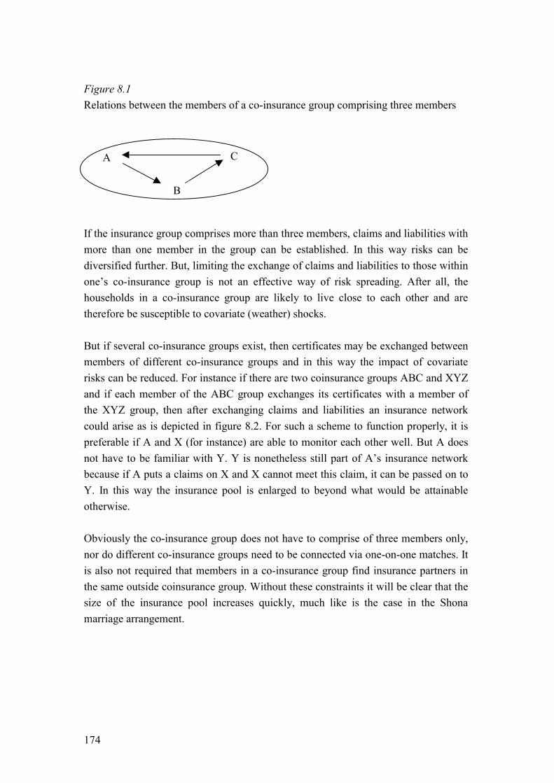
174

Figure 8.1 Relations between the members of a co-insurance group comprising three members If the insurance group comprises more than three members, claims and liabilities with more than one member in the group can be established. In this way risks can be diversified further. But, limiting the exchange of claims and liabilities to those within one�s co-insurance group is not an effective way of risk spreading. After all, the households in a co-insurance group are likely to live close to each other and are therefore be susceptible to covariate (weather) shocks. But if several co-insurance groups exist, then certificates may be exchanged between members of different co-insurance groups and in this way the impact of covariate risks can be reduced. For instance if there are two coinsurance groups ABC and XYZ and if each member of the ABC group exchanges its certificates with a member of the XYZ group, then after exchanging claims and liabilities an insurance network could arise as is depicted in figure 8.2. For such a scheme to function properly, it is preferable if A and X (for instance) are able to monitor each other well. But A does not have to be familiar with Y. Y is nonetheless still part of A�s insurance network because if A puts a claims on X and X cannot meet this claim, it can be passed on to Y. In this way the insurance pool is enlarged to beyond what would be attainable otherwise. Obviously the co-insurance group does not have to comprise of three members only, nor do different co-insurance groups need to be connected via one-on-one matches. It is also not required that members in a co-insurance group find insurance partners in the same outside coinsurance group. Without these constraints it will be clear that the size of the insurance pool increases quickly, much like is the case in the Shona marriage arrangement.

A

B

C

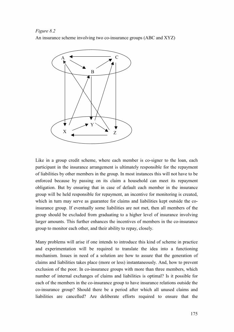
175

Figure 8.2 An insurance scheme involving two co-insurance groups (ABC and XYZ) Like in a group credit scheme, where each member is co-signer to the loan, each participant in the insurance arrangement is ultimately responsible for the repayment of liabilities by other members in the group. In most instances this will not have to be enforced because by passing on its claim a household can meet its repayment obligation. But by ensuring that in case of default each member in the insurance group will be held responsible for repayment, an incentive for monitoring is created, which in turn may serve as guarantee for claims and liabilities kept outside the co-insurance group. If eventually some liabilities are not met, then all members of the group should be excluded from graduating to a higher level of insurance involving larger amounts. This further enhances the incentives of members in the co-insurance group to monitor each other, and their ability to repay, closely. Many problems will arise if one intends to introduce this kind of scheme in practice and experimentation will be required to translate the idea into a functioning mechanism. Issues in need of a solution are how to assure that the generation of claims and liabilities takes place (more or less) instantaneously. And, how to prevent exclusion of the poor. In co-insurance groups with more than three members, which number of internal exchanges of claims and liabilities is optimal? Is it possible for each of the members in the co-insurance group to have insurance relations outside the co-insurance group? Should there be a period after which all unused claims and liabilities are cancelled? Are deliberate efforts required to ensure that the

A

B

C

X Y

Z

176

arrangement is contingent? Or does the fact that households hold more than one claim imply that households will carry out a means test themselves in order to increase the probability of speedy repayment. If this is true, the arrangement will automatically become conditional. On the other hand to avoid refusal to participate one might have to ensure beforehand that the obligation to repay debt is conditional on possessing sufficient income (or outstanding claims). These and many other issues will have to be resolved before any claims and liabilities arrangement can be implemented in practice. Nevertheless seeking solutions for these issues is worthwhile, especially if it contributes to the reduction of the impact of risk on the lives of Zimbabwe�s rural population.

Summary in Dutch

Samenvatting

9.1 Inleiding Risico�s kunnen niet altijd worden vermeden. We worden ziek, oud of raken onze baan kwijt. In een land als Nederland zijn de financiële gevolgen van dit soort risico�s verzekerd. Ziekenkosten worden vergoed, in geval van ouderdom ontvangen we AOW en bij werkeloosheid een uitkering. Toch heeft elk van deze gebeurtenissen vaak ingrijpende materiële en immateriële gevolgen. Als dit al zo is in een rijk land als Nederland, hoeveel groter zijn de gevolgen van risico dan op het platteland van Zimbabwe waar de risico�s groter zijn en verzekeringen veelal ontbreken. Om een indruk te krijgen van de risico�s waarmee Zimbabwaanse boeren te maken krijgen en de manier waarop zij de gevolgen daarvan proberen te beperken wordt in paragraaf 9.2 een illustratie gegeven van een hypothetisch boerenhuishouden. Uiteraard is het voorbeeld niet willekeurig gekozen, maar bevat het aspecten die in dit proefschrift aan de orde komen. In paragraaf 9.3 volgt de samenvatting van het Engelstalige deel van dit proefschrift.

178

9.2 Uit het Leven van een Zimbabwaanse Boer

Een pas getrouwd stel begint te boeren met de twee koeien die de echtgenoot bijeen wist te sparen in de jaren voor het huwelijk. Het echtpaar verbouwt maïs, dat vooral gebruikt wordt voor de eigen consumptie, en katoen. Hoewel het stel in een afgelegen gebied woont, wonen ze niet zo geïsoleerd dat zij geen onderdeel uitmaken van de rest van de economie. Eens per jaar wordt het overschot aan maïs en de katoen verkocht aan handelaren of aan het desbetreffende staatsbedrijf. Van het geld dat op deze manier wordt verkregen worden zaden, kunstmest, pesticide en andere essentiële goederen gekocht. Het geld dat overblijft wordt opzij gezet om schoolgeld te betalen, om buskaartjes te kopen en om een potje te vormen voor onverwachte uitgaven. Voor de zekerheid wordt een deel van de maïsoogst bewaard. Dit dient als buffer voor slechte periodes. Daarnaast probeert het huishouden meer koeien te krijgen. Koeien kunnen worden verkocht wanneer er plotseling geld nodig mocht zijn. Daarnaast is hun trekkracht nodig om te ploegen en om de ossenwagen te trekken. Verder geven koeien melk, verbetert hun mest de vruchtbaarheid van de grond en vermenigvuldigen ze zich. Het hebben van koeien is daarom belangrijk. Het land dat bebouwd wordt is niet geïrrigeerd en met de regenval varieert de oogst. De opbrengst van het land wisselt niet alleen van jaar tot jaar, hij varieert ook tussen huishoudens in het dorp. Het echtpaar wil niet dat de hoogte van de consumptie afhankelijk is van de omvang van de oogst. En door te sparen in goede jaren en de besparingen te consumeren na een minder goede oogst wordt een gelijkmatiger consumptiepatroon bereikt. Ook wordt er samengewerkt met dorpsgenoten. Van buren met een goede oogst krijgt het stel geschenken in jaren waarin het zelf pech heeft gehad. In jaren waarin een goede oogst is behaald, delen de buren mee in de voorspoed. Op deze manier verzekeren de dorpsgenoten elkaar. Door hard te werken, zuinig te leven en te fokken lukt het om het aantal koeien te laten stijgen van twee naar vijf, de kinderen naar school te sturen en tegenslagen als ziekte en tegenvallende regenval op te vangen. Dan verzoekt de schoonvader de echtgenoot een deel van de nog openstaande bruidsprijs te betalen. Om aan dit verzoek te voldoen, geeft hij zijn schoonvader twee koeien. Deze laatste gebruikt de ontvangen koeien als aanbetaling voor het huwelijk van zijn eigen zoon. In het daarop volgende jaar gaat een koe dood van ouderdom en wordt er een kalf geboren. Als een van de kinderen vervolgens ernstig ziek wordt, wordt dit kalf verkocht om de doktersrekening te betalen. Het stel bezit nu een koe en een os, precies genoeg om te kunnen ploegen.

179

Om te voorkomen dat de inmiddels zwangere koe haar vrucht verliest door de inspanning van het ploegen wordt besloten haar te ontzien bij het bewerken van het land. In plaats daarvan wordt, om toch te kunnen ploegen, samengewerkt met dorpsgenoten die in een vergelijkbare situatie zitten. Door elkaars ossen te gebruiken kan toch worden geploegd. Het gevolg is wel dat niet al het land op tijd gereed is om ingezaaid te worden en dat minder land dan normaal bebouwd kan worden. Het stel verwacht dan ook minder dan normaal te zullen oogsten. Maar als de koe een gezond kalf zou baren, is dit het meer dan waard. Helaas, wordt de zwangere koe gestolen. Na de oogst, die niet al te groot is, is het echtpaar niet in staat een extra koe te kopen, tenzij de kinderen van school gehaald zouden worden (dit bespaart immers schoolgeld). Dat laatste willen ze niet en het stel gaat door het land te bewerken met gebruikmaking van hun enige os. Ondanks het lage inkomen wordt nog altijd actief deelgenomen aan informele dorpsverzekeringen. Dit om beschouwd te worden als goede buur en in de verwachting dat dit bijdraagt aan het ontvangen van trekkracht tijdens het plantseizoen. Daarnaast besluit de zoon zijn vader om hulp te vragen. Immers, traditioneel verzorgt de vader de bruidsprijs van zijn zoon. In dit geval kan zou de vader zijn zoon ook redelijk gemakkelijk tegemoet moeten kunnen komen omdat hijzelf nog een deel van de bruidsprijs van zijn dochters tegoed heeft van zijn schoonzoons. Dan komt er een droogte en de oogst van eenieder in het dorp mislukt. In hun pogingen te overleven verkopen de rijkere dorpsgenoten koeien. Met de opbrengst daarvan wordt vervolgens voedsel gekocht. Ons echtpaar kan dit ook doen, maar zou dan wel hun enige os verliezen. Ze besluiten dit niet te doen en in plaats daarvan te vertrouwen op de solidariteit van de rijkere dorpsbewoners. Maar terwijl de droogte voortduurt en de beschikbare middelen verder afnemen, geven de rijkeren er de voorkeur aan hun informele verzekering exclusief onder elkaar te houden. Zij blijken niet bereid koeien te verkopen ten bate van hun arme buren omdat ze verwachten deze koeien zelf nodig te hebben na de droogte. Nu de kaarten zo geschud zijn, heeft het echtpaar geen keus en wordt de os verkocht. Dit ondanks de inmiddels dramatisch lage prijs. Daarnaast worden de kinderen van school gehaald en rest er niets anders dan te hopen op hulp van buitenaf. Na de droogte herstellen de rijkere huishoudens � en zeker zij die nog in staat zijn te ploegen, zich binnen korte tijd. Dit geldt niet voor het echtpaar dat geen enkele trekkracht meer bezit. Hen rest niets anders dan het land met de hand te bewerken. Het inkomen dat nu met landbouw wordt verdiend is erg laag, en om het aan te vullen verzorgen de kinderen de koeien van rijkere dorpsgenoten. Vanzelfsprekend probeert

180

het echtpaar ook te sparen om twee nieuwe koeien te kopen maar nu het inkomen laag is, is het vrijwel onmogelijk om het benodigde geld bijeen te brengen. Ook wordt geprobeerd koeien te lenen. Maar nu zij zelf geen os kunnen inbrengen behoort het echtpaar tot de laatsten die aanspraak kunnen maken op trekkracht. Tegen de tijd dat er koeien beschikbaar komen is de tijd om te planten eigenlijk al voorbij en zijn de koeien uitgeput van het zware werk op het land. Het echtpaar leeft dan ook gedurende een langere periode in grote armoede. Pas wanneer de vader van de echtgenoot een koe krijgt van een van zijn schoonzoons (nadat deze laatste van de droogte is hersteld), en hij haar doorgeeft aan zijn zoon, onstaat er weer uitzicht op verbetering van de situatie. Inmiddels zijn de kinderen al een aantal jaar niet naar school gegaan en is het onwaarschijnlijk dat zij hier ooit naartoe zullen terugkeren. Dit voorbeeld laat een veelheid aan risicofactoren zien. Droogte, ziekte, diefstal, sterfte van koeien en sociale uitsluiting maken het leven op het platteland onvoorspelbaar. Niet alle risico�s hebben dramatische gevolgen. De kosten van de ziekte konden worden opgevangen door de verkoop van een kalf. Maar in andere gevallen (en zeker na een reeks vervelende voorvallen) leidt risico tot grote ellende. Tijdens de droogte wordt er honger geleden en de kinderen van het echtpaar worden blijvend in hun ontplooiingsmogelijkheden geschaad daar zij van school gehaald worden en daar niet naar terugkeren. Het voorbeeld illustreert verschillende manieren waarop de gevolgen van risico beperkt kunnen worden. Door graan op te slaan, geld te sparen, samen te werken met dorpsgenoten en door koeien te verkopen kunnen de ergste gevolgen van tegenslagen vermeden worden. Er zit ook een keerzijde aan de verschillende vormen van verzekeren. Tijdens de droogte wordt het inmiddels arme huishouden uitgesloten van de informele dorpsverzekering. Omdat koeien ook gebruikt worden als trekkracht is het huishouden niet bereid ze in een vroeg stadium (wanneer de prijs nog redelijk is) te verkopen. En als alle koeien eenmaal verdwenen zijn, wordt het moeilijk om een redelijk inkomen te verdienen. Voor dit probleem bestaat ook een oplossing. Dankzij de assistentie van de vader en zijn recht op koeien van zijn schoonzoons, is het mogelijk dat het echtpaar zich toch ook weer aan deze armoedeval ontworstelt. Het voorbeeld kan ook gebruikt worden als illustratie voor het feit dat een formele verzekering veel voordelen biedt. Wanneer het echtpaar verzekerd zou zijn geweest tegen diefstal, was de kans op uitsluiting tijdens de droogte kleiner geweest. En wanneer tijdens de droogte geld of voedsel zou zijn ontvangen, was er geen noodzaak geweest de armsten uit te sluiten van de informele verzekering, en had de grootschalige verkoop van koeien, die later weer nodig zijn voor productie, voorkomen kunnen worden.

181

9.3 Risico en Verzekeren op het Platteland van Zimbabwe: Samenvatting

In hoofdstuk 2 wordt een overzicht gegeven van verschillende manieren om met risico om te gaan. Een mogelijkheid is door zich te verzekeren. Als het inkomen volledig verzekerd is, kunnen boeren zich specialiseren in die activiteit die de hoogste gemiddelde opbrengst oplevert, ongeacht de fluctuaties in die opbrengst. Dit is mogelijk omdat een verzekering inkomensfluctuaties van veel agenten poolt. Vanwege de wet van de grote getallen middelen goede en slechte uitkomsten uit en kan iedere deelnemer aan de verzekering zijn gemiddelde opbrengst krijgen. Dit werkt alleen als veel verschillende risico�s gepoold worden, hetgeen de reden is waarom verzekeringen door bedrijven of door de overheid aantrekkelijk zijn: zij zijn in staat veel verschillende risico�s in een verzekering onder te brengen. Volledige verzekeringen bestaan echter niet en op het platteland van Zimbabwe worden zelfs in het geheel geen verzekeringsdiensten aangeboden. Dit betekent dat boeren zelf verzekeringsoplossingen moeten vinden. Voor een deel gebeurt dit binnen de familie of binnen het dorp. Familieleden helpen elkaar en hetzelfde geldt voor buren en dorpsgenoten. Nadeel van verzekeren binnen kleine kring is dat als iedereen getroffen wordt door een laag inkomen (bijvoorbeeld tijdens een droogte), er geen goede opbrengsten zijn om de slechte te compenseren. Verzekeren heeft dan weinig zin. Daarnaast moet misbruik voorkomen worden. Zij die een goede oogst hebben moeten gedwongen kunnen worden een deel daarvan af te staan om hen die pech hebben gehad te compenseren (enforcement). Aan de andere kant moet het ook zeker zijn dat tegenslag niet ontstaan is door een gebrek aan inspanning of door onvoorzichtigheid van de deelnemer aan de verzekering (moral hazard). Tenslotte moet voorkomen worden dat bepaalde groepen uitgesloten worden van verzekering. Dit gebeurt bijvoorbeeld wanneer verwacht wordt dat bepaalde deelnemers in de toekomst maar weinig zullen bijdragen aan de pool, terwijl zij er nu wel een kostbaar beroep op doen. In het voorbeeld in de vorige paragraaf gebeurde dit toen het inmiddels arme huishouden uitgesloten werd van steun. Het dacht geholpen te zullen worden, maar de rijkere huishoudens weigerden dit omdat zij het geven van steun tijdens een droogte als te kostbaar beschouwden in vergelijking met de opbrengt daarvan, namelijk dat het arme huishouden onderdeel blijft uitmaken van de verzekeringspool. Dat armen uitgesloten worden van informele verzekeringen tijdens een negatieve inkomensschok is een bekend en zorgwekkend fenomeen.

182

In plaats van elkaar te verzekeren kunnen boeren ook proberen inkomensrisico�s te spreiden door diversificatie. Bijvoorbeeld door gewassen met verschillende eigenschappen te verbouwen. Of door een deel van het inkomen buiten de landbouw te verdienen. Diversificatie gaat echter ten koste van specialisatie en is daarom duur. Een andere mogelijkheid is sparen. Door te sparen in goede jaren zijn er in slechte jaren toch middelen beschikbaar voor consumptie. In theorie kunnen besparingen ervoor zorgen dat de invloed van inkomensschokken op de consumptie sterk vermindert. Maar daarvoor is wel een ideaal spaarmiddel nodig. Dat wil zeggen een goed dat binnen redelijke termijn geruild kan worden zonder waardeverlies, waarvan de waarde niet daalt als er een schok plaatsvindt, dat in kleine hoeveelheden aangehouden kan worden en dat een positieve rente genereert. De spaarmiddelen waarover de boeren in de praktijk kunnen beschikken zijn niet van het ideale type. De meest gebruikte spaarvormen zijn het opslaan van graan, bewaren van geld en het houden van koeien. Met name deze laatste manier is populair in Zimbabwe. De reden daarvoor is dat, anders dan graan dat elk jaar minder waard wordt, koeien zich vermenigvuldigen. Koeien kunnen ook gebruikt worden om te ploegen, geven melk en mest, en kunnen geruild worden tegen voedsel wanneer dat nodig is. Nadeel van het gebruik van koeien is dat als velen proberen koeien te verkopen, bijvoorbeeld ten tijde van droogte, dat de prijs dan sterk daalt zodat maar weinig voedsel voor de verkochte koeien kan worden gekocht. Een ander nadeel is dat huishoudens zullen proberen het verkopen van koeien te voorkomen. De beesten zijn immers van belang als trekkracht in de periode na de droogte. Hierdoor kan het gebeuren dat huishoudens met voldoende besparingen toch hun consumptie sterk verminderen tijdens een periode waarin weinig verdiend wordt. Tenslotte kan er ook gebruik gemaakt worden van krediet. Door geld te lenen als het slecht gaat en dit terug te betalen wanneer het goed gaat kan het huishouden zijn consumptie op peil houden tijdens inkomensschokken. Op het platteland van Zimbabwe wordt echter geen krediet voor consumptieve doeleinden verstrekt. De belangrijkste redenen hiervoor zijn dat de bedragen die boeren willen lenen te klein zijn voor banken om interessant te zijn, en dat boeren meestal geen onderpand kunnen verstrekken. Dit proefschrift maakt gebruik van gegevens die verzameld zijn onder leiding van Bill Kinsey. In hoofdstuk 3 worden de data beschreven. De gebruikte informatie is bijzonder omdat het gegevens zijn voor 400 boeren huishoudens uit Zimbabwe�s landhervormingsprogramma, en vooral omdat sinds 1992 elk jaar opnieuw dezelfde huishoudens soortgelijke vragen hebben beantwoord. Daarmee is een panel dataset ontstaan die door zijn lengte uniek is voor Afrika. Door telkens terug te gaan naar

183

dezelfde huishoudens is het mogelijk een goed beeld te vormen hoe boeren met risico omgaan. Daarmee is deze data set erg geschikt voor onderzoek naar risico en verzekeren. Nadeel van het gebruik van Kinsey�s gegevens is dat boeren in een landhervormingsprogramma niet representatief zijn voor alle boeren in Zimbabwe. Maar ook dit nadeel heeft zo zijn voordeel. Door de manier waarop de geïnterviewde boeren leven, in een geïsoleerd gebied, zonder financiële markten en met veel grond zonder dat daar eigendomsrechten voor bestaan, lijken ze erg op wat soms als Afrikaanse boer gestereotypeerd wordt (Binswanger and McIntire, 1987). Om de grootste nadelen van non-representativiteit te ondervangen zijn sinds 1997 ook gegevens verzameld onder een groep van 150 �gewone� boeren. Het grootste verschil met de begunstigden uit het landhervormingsprogramma is dat deze boeren minder land bewerken, kleinere huishoudens hebben en voor een belangrijk deel hun inkomen buiten de landbouw verdienen. In hoofdstuk vier wordt de vraag gesteld waarom inkomensverzekeringen eigenlijk niet worden aangeboden op het platteland van Zimbabwe. Immers boeren lopen een groot inkomensrisico zodat het voor de hand ligt dat zij zich hiertegen zouden willen beschermen. Een mogelijk verklaring is dat het wel meevalt met dit risico. Dit blijkt niet te kloppen. De variatiecoëfficiënt van het inkomen is gemiddeld 40 � 60 procent, hetgeen betekent dat als de consumptie net zo erg zou fluctueren als het inkomen, boeren bereid zouden zijn 8 tot 36 procent65 van hun gemiddeld inkomen te betalen voor een verzekering die hun een gelijkmatig inkomen garandeert! Dit is een groot bedrag, zeker gezien het feit dat deze boeren niet rijk zijn. Deze marge lijkt ook voldoende groot om oplossingen te vinden voor moral hazard en enforcement problemen zodat het mogelijk zou moeten zijn voor verzekeringsmaatschappijen om winstgevend te opereren. Waarom worden dergelijke verzekeringen dan toch niet aangeboden? Het kan natuurlijk zijn dat de vraag naar verzekeringen kleiner is dan gedacht, omdat boeren zelf in staat zijn ervoor te zorgen dat hun consumptie minder varieert dan het inkomen. In hoofdstuk twee zijn de mogelijkheden al genoemd: boeren kunnen sparen en ontsparen of ze kunnen elkaar verzekeren (deze laatste mogelijkheid wordt in hoofdstuk 5 onderzocht). Daarnaast sparen huishoudens vooral, zo blijkt in dit hoofdstuk, door het aanhouden van voedselvoorraden, het hebben van cash en door vee te accumuleren. Ongeacht hoe men zich verzekert, de variatiecoëfficiënt van de consumptie blijkt 25 � 35 procent te zijn. Dit is hoog, vooral omdat dit gevonden wordt voor een periode

65 Afhankelijk van de mate van relatieve risico-aversie.

184

waarin zich geen grote droogtes hebben voorgedaan. Huishoudens met een dergelijke variatie in hun consumptie zijn bereid 4 tot 12 procent van hun gemiddelde consumptie op te offeren voor een verzekering die hun een gelijkmatige inkomensstroom garandeert. Om er zeker van te zijn dat 25-35 procent een realistische schatting van de consumptievariatie is, wordt in hoofdstuk 4 ook langs andere weg geprobeerd te achterhalen wat de minimale consumptievariatie zou zijn wanneer een huishouden de beschikking zou hebben over een ideaal spaarmiddel. Aan de hand van een theoretisch model en met behulp van een numerieke oplossingsmethode wordt de optimale consumptiestrategie bepaald voor een huishouden wiens tijdsvoorkeurvoet hoger is dan de opbrengst van besparingen. Vervolgens is met behulp van de Monte Carlo techniek vastgesteld wat de optimale minimale consumptievariatie zou zijn in het geval huishoudens de beschikking hebben over de ideale spaarvorm. De uitkomst is dat onder die omstandigheden de coëfficiënt van de consumptievariatie 13 - 20 procent zou zijn. Dit laat zien dat een spaarstrategie eigenlijk heel goed werkt, mits er goede spaarvormen bestaan. Aangezien een ideale spaarvorm niet bestaat wordt de gevonden variatie van 25-35 procent realistisch geacht. Wat betekent dit nu voor de vraag waarom verzekeringsmaatschappijen geen diensten aanbieden op het platteland van Zimbabwe. Het lijkt er in ieder geval op dat er voldoende vraag naar inkomensverzekeringen is om de kosten die een verzekeraar zou moeten maken te kunnen dekken. Dit doet de vraag rijzen of er nog andere redenen zouden kunnen zijn die het onaantrekkelijk maken een verzekering aan te bieden. Een mogelijkheid (en aanwijzingen hiervoor heb ik gekregen in gesprekken met boeren) is dat boeren er maar weinig vertrouwen in hebben dat een verzekeringsmaatschappij daadwerkelijk tot uitbetaling over zal gaan. Feitelijk is dit een andere manifestatie van het al eerder genoemde enforcement probleem. In hoofdstuk 5 wordt nagegaan in hoeverre verschillende informele verzekeringsvormen bijdragen aan grotere consumptiezekerheid. Daartoe wordt een toets ontwikkeld die rekening houdt met het feit dat boeren, om een gelijkmatig inkomenspatroon te krijgen, niet alleen gebruik maken van informele verzekeringen maar ook van besparingen (dit bleek uit hoofdstuk 4). In een theoretische afleiding wordt duidelijk dat in plaats van de gebruikelijk toets, waarbij getest wordt of de consumptie wordt verklaard door het totaal van de dorpsconsumptie en onafhankelijk is van het eigen inkomen, getest zou moeten worden of huishoudconsumptie wordt verklaard door het totaal van de dorpsconsumptie en onafhankelijk is van het eigen inkomen en de omvang van het vermogen van een huishouden.

185

Met behulp van deze toets wordt een aantal zaken onderzocht. Is er sprake van volledige verzekering? Is de mate van verzekeren anders voor armen dan voor rijken, is het anders voor boeren uit het landhervormingsprogramma dan voor �gewone� boeren en vindt verzekering vooral plaats binnen het dorp of binnen een ruimer sociaal verband? De toets is op twee manier uitgevoerd. Niet alleen wordt getest of huishoudconsumptie wordt verklaard door het totaal van de dorpsconsumptie en onafhankelijk is van het eigen inkomen en de omvang van het vermogen van het huishouden maar ook of de huishoudbesparingen worden verklaard door het huishoudinkomen en het totaal van de dorpsconsumptie en onafhankelijk zijn van de hoogte van het vermogen van het huishouden. Beide toetsen leveren vergelijkbare resultaten op. Er wordt gevonden dat de bestaande informele verzekeringssystemen gedeeltelijke bescherming bieden tegen inkomensschokken, en dat de mate van bescherming niet afhangt van deelname aan het landhervormingsprogramma. Ook wordt er gevonden dat de mate van verzekeren net zo groot is op dorpsniveau als voor het hele gebied van de enquête. De conclusie die hieraan verbonden wordt, is dat als volledige informele verzekering bestaat, het relevante sociale verband waarbinnen dit gebeurt anders gedefinieerd moet worden dan als het dorp of het gebied van de enquête. Aanwijzingen dat de relevante verzekeringsgroep bestaat uit dorpsgenoten en familieleden die elders wonen zijn wel gevonden, maar de informatie voor een formele test voor deze groep ontbrak. Tenslotte wordt gevonden dat de armen in dezelfde mate verzekerd zijn als de rijkeren. Dit is een geruststelling. Uit het voorbeeld in de vorige paragraaf bleek dat het goed mogelijk is dat de rijkeren armen uitsluiten van verzekering. Hiervoor zijn geen aanwijzingen gevonden. Toch is dit nog geen reden voor vreugde omdat zich tijdens de periode waarvoor de toets is uitgevoerd zich geen grote schokken hebben voorgedaan. En juist wanneer dit het geval is komen informele verzekeringssystemen onder druk te staan. Helaas ontbraken de gegevens om dezelfde toets uit te voeren voor jaren waarin zich wel grote schokken hebben voorgedaan. Uit de hoofdstukken 4 en 5 volgt is dat het inkomen van boerenhuishoudens in Zimbabwe sterk fluctueert, maar dat zij in staat zijn de ergste consumptieve gevolgen hiervan te vermijden door gebruik te maken van besparingen en door informele verzekeringssystemen. Desondanks blijft er vraag naar een additionele verzekeringen door een betrouwbare verzekeringsmaatschappij. Regenval is aangemerkt als belangrijke bron van risico terwijl koeien zijn vooral een manier om de gevolgen van risico�s af te dekken. In hoofdstuk 6 wordt aangetoond dat koeien ook een bron van risico zijn. In hoofdstuk 7 komt vervolgens een verzekeringsmechanisme aan de orde dat dit risico afdekt.

186

In hoofdstuk 6 wordt het belang van trekkracht voor het verwerven van inkomen uit de landbouw onderstreept. In het beschrijvende deel van dit hoofdstuk wordt aannemelijk gemaakt dat door gebruik te maken van koeien, boeren meer land in gebruik kunnen nemen. Ook brengt het land dan meer op. Dit maakt het mogelijk dat boeren die niet over koeien beschikken en die hun land met de hand moeten bewerken, zo weinig verdienen dat zij niet in staat zijn om voldoende geld te sparen om koeien aan te schaffen. In het theoretische deel van hoofdstuk 6 wordt aangetoond dat als er geen banken zijn waar geld geleend kan worden en er inderdaad een minimum hoeveelheid kapitaalgoederen nodig is om een redelijk inkomen te verwerven (twee koeien) het mogelijk is dat boeren in een armoedeval terechtkomen. In het empirische gedeelte van hoofdstuk 6 worden twee zaken getoetst. Allereerst wordt gekeken of een van de voorspellingen van het model ook in de praktijk gevonden wordt. Het model voorspelt dat als een armoedeval bestaat, boeren of geen koeien hebben, of tenminste twee. Empirisch wordt deze verdeling van het aantal koeien bevestigd. De tweede toets bekijkt of de productiefunctie inderdaad zo is dat boeren zonder koeien weinig land in gebruik nemen en dat boeren met tenminste twee koeien meer land bewerken. Dit wordt getest in een regressieanalyse. De resultaten tonen aan dat dit het geval is voor de boeren uit het landhervormingsprogramma. Voor de andere boeren zijn de bevindingen minder duidelijk. Het kan zijn dat zij minder last hebben van een armoedeval (bijvoorbeeld omdat deze boeren een groot deel van hun inkomen elders verdienen) maar het kan ook zijn dat de resultaten zwak zijn ten gevolge van de gekozen statistische methode (een fixed-effects schatting). Vooral wanneer zich meetfouten voordoen in combinatie met niet al te grote veranderingen van de verklarende variabelen in de tijd, leidt deze methode snel tot niet significante resultaten. Hoe het ook zij, wanneer gekeken wordt hoe lang huishoudens geen koeien hebben, dan kan op basis hiervan geconcludeerd worden dat ongeveer 7 procent van de boeren uit het landhervormingsprogramma in een armoedeval zit. Voor de andere boeren is dit percentage hoger. Overigens gebeurt het regelmatig dat boeren gedurende een kortere periode geen koeien hebben, waarna zij toch in staat blijken te zijn om te ploegen. Blijkbaar is het mogelijk uit de armoedeval te ontsnappen. De illustratie in paragraaf 9.2 heeft hiervan al een idee gegeven, wanneer de vader zijn zoon die geen koeien heeft, een koe geeft. Dit is een vorm van verzekeren.

187

In hoofdstuk 7 wordt hier verder op ingegaan. In dit hoofdstuk wordt aangetoond dat het vragen van een bruidsprijs voor een dochter die gaat trouwen een vorm van verzekeren is. Dit werkt als volgt. Als een zoon gaat trouwen wordt in principe de bruidsprijs die betaald moet worden opgebracht door zijn vader. Een deel van deze bruidsprijs wordt betaald als onderdeel van de huwelijksvoltrekking. De rest wordt later voldaan op momenten waarop de vader van de bruid om koeien verlegen zit en de schoonzoon koeien kan missen. In deze relatie, die afhankelijk is van de welstand van zowel de gever als de ontvanger, zit een verzekeringselement. Het nadeel is dat in dit geval de verzekeringspool slechts uit twee personen bestaat. Maar, de vader heeft niet alleen recht op koeien, hij wordt ook geacht ze te geven wanneer een van zijn zoons gaat trouwen. Een vader bezit dus zowel rechten als verplichtingen. Dit vergroot de pool omdat het nu mogelijk is een claim door te geven. Bijvoorbeeld, als A, B vraagt een deel van zijn bruidsprijs terug te betalen en B (of zijn vader) kan niet aan dit verzoek voldoen dan kan B (B�s vader) als hij nog wat te goed heeft van C, hetzelfde vragen aan C. Als C (of zijn vader) ook niet aan deze wens kan voldoen, maar C (C�s vader) krijgt nog koeien van D en D is in staat de koeien te leveren dan vindt er een feitelijk overdracht van koeien plaats van D naar A. Op deze manier wordt het aantal deelnemers in de verzekering groot en verbetert het functioneren daarvan. Overigens hoeven de ontvangen koeien niet alleen gebruikt te worden om aan de armoedeval te ontkomen. Ze kunnen ook geruild worden tegen voedsel. In het empirische deel van hoofdstuk 7 wordt aangetoond dat het grootste deel van de bruidsprijs niet wordt voldaan op het moment van het huwelijk, maar dat deze langzamerhand wordt terugbetaald. Volledige betaling kan een heel leven duren. Daarbij gaat het hier niet over kleine bedragen. Het totale bedrag aan claims en verplichtingen is ongeveer een kwart van het inkomen dat gedurende een heel leven wordt verdiend! Regressieanalyse toont aan dat het gebruik van verplichtingen en claims afhangt van de economische welstand van het huishouden. Huishoudens die relatief rijk zijn geven eerder koeien en arme huishoudens krijgen ze eerder. Overigens blijkt dat vooral de boeren uit het landhervormingsprogramma gebruik maken van dit systeem. Dit is opmerkelijk omdat er geen aanwijzingen zijn dat het trouwsysteem anders is voor de boeren buiten het landhervormingsprogramma. Maar deze laatsten zijn wel minder afhankelijk van de landbouw, zodat zij er minder belang bij hebben het systeem te gebruiken op een manier die in overeenstemming is met de noodzaak om te kunnen ploegen. In hoofdstuk 7 wordt verder nog ingegaan op het functioneren van deze trouwverzekering. Er wordt aangetoond dat arme boeren niet van deze verzekering uitgesloten worden. Wel huwen dochters uit arme huishoudens op jongere leeftijd. Daarnaast wordt ingegaan op enforcement mechanismen. Traditionele rechtspraak en

188

dreigen met ontevreden voorvaderen of om zijn dochter met haar kinderen terug te halen, moeten de schoonzoon ervan overtuigen dat de bruidsprijs afgelost dient te worden wanneer dit wordt gevraagd. In hoofdstuk 8 wordt een samenvatting gegeven van de bevindingen. Op basis hiervan worden enkele suggesties gedaan over hoe de omstandigheden van Zimbabwaanse boeren verbeterd zouden kunnen worden. Deze suggesties behelzen vooraleerst een verbetering van de economische situatie in het algemeen. Lagere inflatie maakt geld beter geschikt als spaarmiddel. Hogere economische groei schept mogelijkheden voor inkomensdiversificatie buiten de landbouw. Scherper toezicht maakt verzekeringsmaatschappijen geloofwaardiger en betrouwbaarder. Uit hoofdstuk 4 is gebleken dat besparingen een goede manier zijn om het huishouden te beschermen tegen inkomensschokken. Om de situatie van boeren te verbeteren kan dan ook gedacht worden aan verbeteringen in de markten voor vermogenstitels (koeien, geld, goud), zoals het vergroten van de toegang tot de internationale vleesmarkt. Maar ook de particuliere sector kan een bijdrage leveren, bijvoorbeeld door wel verzekeringen aan te bieden op het platteland van Zimbabwe. In hoofdstuk 4 is al vastgesteld dat er een vraag is naar inkomensverzekeringen. Gegeven de specifieke omstandigheden op het platteland van Zimbabwe (vooral de hoge kosten die gemaakt moeten worden om moral hazard te voorkomen) zullen er dan wellicht nieuwe verzekeringsvormen gebruikt moeten worden. Hiertoe worden twee suggesties gedaan. Een daarvan maakt gebruik van de regenval om vast te stellen of huishoudens recht hebben op een uitkering. De ander maakt gebruik van de mechanismen van het trouwsysteem uit hoofdstuk 7.

References Agarwal B. 1990. Social Security and the Family: Coping with Seasonality and Calamity in Rural India. Journal of Peasant Studies 17(3): 341-412. Aghion P. and P. Bolton 1997. A Theory of Tickle Down Growth and Development. Review of Economic Studies 64(2): 151-172. Alderman H. and C. Paxson 1992. Do the Poor Insure? (Washington D.C.: World Bank Working Paper Series 1008). Antle J.M. 1987. Econometric Estimation of Producers' Risk Attitudes. American Journal of Agricultural Economics 69(3): 509-522. Arnott R. and J.E. Stiglitz 1991. Moral Hazard and Nonmarket Institutions: Dysfunctional Crowding Out or Peer Monitoring? American Economic Review 81(1): 179-190. Baerends E.A. 1991. The One-Legged Chicken in the Shadow of Indebtedness: Indebtedness and Social Relationships Among the Anufom of Northern Togo. (Groningen: Groningen University Thesis). Bakker E.J. 1992. Rainfall and Risk in India�s Agriculture: An ex-ante evaluation of rainfall insurance. (Groningen: Wolters-Noordhoff). Banerjee A.V. and A.F. Newman 1991. Risk Bearing and the Theory of Income Distribution. Review of Economic Studies 58(2): 211-235. Banerjee A. and A. Newman 1993. Occupational Choice and the Process of Development. Journal of Political Economy 101(2): 274-298. Bauer P. and F. Paish 1952. The Reduction of Fluctuations in the Incomes of Primary Producers. Economic Journal 62: 750-780. Behrman J. 1988. Intrahousehold Allocation of Nutrients in Rural India: Are Boys Favored? Do Parents Exhibit Inequality Aversion? Oxford Economic Papers 40 (1): 32-54.

Besley T. 1995. Nonmarket Institutions for Credit and Risk Sharing in Low-Income Countries. Journal of Economic Perspectives 9(3): 115-27. Bevan D.L., P. Collier and J.W. Gunning with A. Bigsten and P. Horsnell 1989. Peasants and Governments: An Economic Analysis. (Oxford: Clarendon Press). Bhalla S.S. 1979. Measurement Errors and the Permanent Income Hypothesis: Evidence from Rural India. American Economic Review 69(3): 295-307. Bhalla S.S. 1980. The Measurement of Permanent Income and its Application to Saving Behavior. Journal of Political Economy 88(4): 722-743. Binswanger H.P. and M.R. Rosenzweig 1986. Behavioural and Material Determinants of Production Relations in Agriculture. Journal of Development Studies 22 (3): 503-539. Binswanger H.P. and J. McIntire 1987. Behavioural and Material Determinants of Production Relations in Land Abundant Tropical Agriculture. Economic Development and Cultural Change 36(1): 73-99. Blarel B., P. Hazel and J. Quigging 1992. The Economics of Farm Fragmentation: Evidence from Ghana and Rwanda. World Bank Economic Review 6(2): 233-254. Bourdillon M. 1987. The Shona Peoples. (Gweru: Mambo Press). Caldwell J.C., P.H. Reddy and P.Caldwell 1986. Periodic High Risk as a Cause of Fertility Decline in a Changing Rural Environment: Survival Strategies in the 1980-1983 South Indian Drought. Economic Development and Cultural Change 34(4): 677-701. Cavendish W. 1999. Incomes and Poverty in Rural Zimbabwe during Adjustment: The case of Shindi Ward, Chivi Communal Area. Paper presented at the Centre for Study of African Economies Conference on Poverty in Africa: St Anne�s College, Oxford, April 15th and 16th. Chimedza R. 1994. Rural Financial Markets, chapter 10 in M. Rukuni and C.K. Eicher (eds.) Zimbabwe�s Agricultural Revolution. (Harare: University of Zimbabwe Publications). Cochrane J.H. 1991. A Simple Test of Consumption Insurance. Journal of Political Economy 99(5): 957 � 976. Coate S. and M. Ravallion 1993. Reciprocity without Commitment: Characterization and Performance of Informal Insurance Arrangements. Journal of Development Economics 40(1): 1-24. Collier P., S. Radwan, S. Wangwe and A. Wagner 1986. Labour and Poverty in Rural Tanzania. (Oxford: Clarendon Press). Cox D. and E. Jimenez 1998. Coping with Apartheid: Inter-Household Transfers over the Life-Cycle in South Africa. Boston College and World Bank. Mimeo.

Cox D. and E. Jimenez 1998. Risk-Sharing and Private Transfers: What about Urban Households? Economic Development and Cultural Change 46(3): 621-639. Dasgupta P. and D. Ray 1986. Inequality as a Determinant of Malnutrition and Unemployment: Theory. Economic Journal 96(384): 1011-1034. Datt G. and H. Hoogeveen 2000. El Niño or El Peso? Crisis, Poverty, and Income Distribution in the Philippines. (Washington D.C.: The World Bank, Policy Research Working Papers no. 2466). Deaton A. 1989. Saving in Developing Countries: Theory and Review. Proceedings of the World Bank Annual Conference on Development Economics: 61-108. Deaton A. 1991. Savings and Liquidity Constraints. Econometrica 59(5):1221-1248. Deaton A. 1992. Saving and Income Smoothing in the Cote d�Ivoire. Journal of African Economies 1(1): 1-24. Deaton A. 1997. The Analysis of Household Surveys. A Microeconometric Approach to Development Policy. (Baltimore: Johns Hopkins University Press). Deininger K., J.G.M. Hoogeveen and B.H. Kinsey 2001. Productivity and Equity Impacts of Land Reform: The case of Zimbabwe. Mimeo. Dekker M. and A.J. Hoppenbrouwer 1993. The River Became Their Field: Coping Strategies in a Semi-Arid Area in Zimbabwe. Mimeo. Dekker M. and J.G.M. Hoogeveen 2000. Why Daughters Should Marry. Bride Wealth and Household Security in Zimbabwe. Mimeo. Dercon S. 1992a. The Role of Assets in Coping with Household Income Fluctuations: Some Simulation Results. (Oxford: University of Oxford, Centre for the Study of African Economies). Dercon S. 1992b. Agriculture and Risk. (Oxford: University of Oxford, Centre for the Study of African Economies). Dercon S. 1996. Risk, Crop Choice, and Savings: Evidence from Tanzania. Economic Development and Cultural Change 44(3): 485-513. Dercon S. 1998. Wealth, Risk and Activity Choice: Cattle in Western Tanzania. Journal of Development Economics 55(1): 1-42. Dercon S. and P. Krishnan 1996. Income Portfolios in Rural Ethiopia and Tanzania: Choices and Constraints. Journal of Development Studies 32(6): 850-875. Dercon S. 1999. Income Risk, Coping Strategies and Safety Nets. Mimeo. Drèze J. and A. Sen 1989. Hunger and Public Action. (Oxford: Clarendon Press).

Duncan G. and D. Hill 1984. An Investigation of the Extent and Consequences of Measurement Error in Labor Economic Survey Data. (Ann Harbor: Survey Research Center, University of Michigan). Ellis F. 1998. Household Strategies and Rural Livelihood Diversification. Journal of Development Studies 35(1): 1-38. Eswaran M. and A. Kotwal 1986. Access to Capital and Agrarian Production Organisation. Economic Journal 96(382): 482-498. Fafchamps M. 1992. Solidarity Networks in Preindustrial Societies: Rational Peasants with a Moral Economy. Economic Development and Cultural Change 41(1): 147-174. Fafchamps M. and S. Gavian 1996. The Spatial Integration of Livestock Markets in Niger. Journal of African Economies 5(3): 336-405. Fafchamps M., C. Udry and K. Czukas 1998. Drought and Saving in West Africa: Are Livestock a Buffer Stock? Journal of Development Economics 55(2): 273-305. Galor O. and J. Zeira 1993. Income Distribution and Macroeconomics. Review of Economic Studies 60(1): 35-52. Gautam M., P. Hazell and H. Alderman 1994. Rural Demand for Drought Insurance. (Washington D.C.: Policy Research Working Paper 1383, The World Bank). Gauthier C., M. Poitevin and P. González 1997. Ex Ante Payments in Self-Enforcing Risk-Sharing Contracts. Journal of Economic Theory 76(1): 106-144. Goody J. and S.J. Tambiah 1973. Bridewealth and Dowry. (Cambridge: Cambridge University Press). Grimard F. 1997. Household Consumption Smoothing through Ethnic Ties: Evidence from Côte D�Ivoire. Journal of Development Economics 53(2): 391-422. Gunning J.W., J. Hoddinott, B. Kinsey and T. Owens 2000. Revisiting forever gained: Income Dynamics in the Resettlement Areas of Zimbabwe, 1983-1997. Journal of Development Studies 36(6): 131-154. Hazell P. 1982. Application of Risk Preference Estimates in Firm-Household and Agricultural Sector Models. American Journal of Agricultural Economics 64(2): 384-390. Hoddinott J. and B. Kinsey 1999. Child Growth in the Time of Drought. Mimeo. Holleman J.F. 1975. Shona Customary Law: With Reference to Kinship, Marriage, the Family and the Estate. (Cape Town: Oxford University Press). Hoogeveen H. 1999. Marriage as Informal Insurance against the Loss of Draught Power. Tijdschrift voor Politieke Economie 22(1): 82-104 (in Dutch).

Hoogeveen J.G.M. 2000a. The Puzzle of the Absent Rural Formal Financial Institutions. In A. van Tilburg, H. Moll and A. Kuyvenhoven (eds.). Agricultural Markets Beyond Liberalization. (Boston: Kluwer Academic Publishers). Hoogeveen, J.G.M. 2000b. Risk, Insurance and the Poor. In A. Kreimer and M. Arnold (eds.). Managing Disaster Risk in Emerging Economies. (Washington D.C.: The World Bank, Disaster Risk Management Series no. 2). Hoogeveen J.G.M. and B. H. Kinsey 2001a. Land Reform, Growth and Equity: Emerging Evidence from Zimbabwe�s Resettlement Program: a sequel. Journal of Southern African Studies 27(1): 127-136. Hoogeveen J.G.M. and B. H. Kinsey 2001a. Consequences of Drought and Economic Reform for Communal and Land Reform Households. Mimeo. Hsiao C. 1985. Benefits and Limitations of Panel Data. Econometric Reviews 4(1): 121 - 174. Jacoby H. and E. Skoufias 1997. Risk, Financial Markets and Human Capital in a Developing Country. Review of Economic Studies 64(3): 335-371. Jalan J. and M. Ravallion 1999. Are the Poor Less Well Insured? Evidence on Vulnerability to Income Risk in Rural China. Journal of Development Economics 58(1): 61-81. Jappelli T. and L. Pistaferri 1999. Intertemporal Choice and Consumption Mobility. (Centro Studi Ecomomia E Finanza, CSEF, Working Paper no 23). Johda N.S. 1978. Effectiveness of Farmer�s Adjustment to Risk. Economic and Political Weekly 13(25). Just R. and W. Candler 1985. Production Functions and Rationality of Mixed Cropping. European Review of Agricultural Economics 12(3): 207-231. Kennedy P. 1990. A Guide to Econometrics. (Oxford: Basil Blackwell Ltd.). Kimball M. 1988. Farmers� Cooperatives as Behavior toward Risk. American Economic Review 78(1): 224-232. Kinsey B.H. 1998. Dancing with El Nino: Drought, The State and Nutritional Welfare of Rural Children in Zimbabwe, chapter 12 in H. O�Neill and J. Toye (eds.) A World Without Famine? New Approaches to Aid and Development. (London: Macmillan). Kinsey B., K. Burger and J.W. Gunning 1998. Coping with Drought in Zimbabwe: Survey Evidence on Responses of Rural Households to Risk. World Development 26(1): 89-110. Kinsey B.H. 1999. Land Reform, Growth and Equity: Emerging Evidence from Zimbabwe�s Resettlement Program. Journal of Southern African Studies 25 (2): 173-196.

Kochar A. 1999. Smoothing Consumption by Smoothing Income: Hours-of-Work Responses to Idiosyncratic Agricultural Shocks in Rural India. Review of Economics and Statistics 81(1): 50-61. Krugman P. 1980. Scale Economies, Product Differentiation, and the Pattern of Trade. American Economic Review 70(5): 950-958. Kuper A. 1982. Wives for Cattle; Bridewealth and Marriage in Southern Africa. (London: Routledge). Kuys P.H.M. 1999 Marktconforme Verzekeringsoplossingen. Economisch Statistische Berichten 4193: 14-18. Lanjouw P. and M. Ravallion 1995. Poverty and Household Size. Economic Journal 105(433): 1415-1434. Loef C.E. 2000. The Influence of Inheritance on Livelihood Strategies: the Case of Communal and Resettlement Tenure Systems in Zimbabwe. Mimeo. Lucas R.E.B. and O. Stark 1985. Motivations to Remit: Evidence from Botswana. Journal of Political Economy 93(5): 901-918. Mace B.J. 1991. Full Insurance in the Presence of Aggregate Uncertainty. Journal of Political Economy 99(5): 928-956. Mair L.P. 1977. Marriage. (London: Penguin). Meekers D. 1993. The Noble Custom of Roora: The Marriage Practices of the Shona of Zimbabwe. Ethnology 32(1): 35-53. Middleton J., A. Rassam, C. Bradley and L.L. Rose 1995. Encyclopedia of World Cultures, Volume IX Africa and The Middle East. (Boston: G.K. Hall & Co). Morduch J. 1999. The Microfinance Promise. Journal of Economic Literature 37(4): 1569-1614. Moyo N., C.M. Matanyaire and A. Norton 1992. Tillage Systems, Farm Machinery and Implements. Chapter 6 in E.E. Whingwiri, M.K. Rukuni, M. Mashingaidze and C.M. Matanyaire (eds.) Small-Scale Agriculture in Zimbabwe. (Harare: Rockwood Publishers). Moyo S. 1995. The Land Question in Zimbabwe. (Harare: SAPES Books). Muir K. 1994. Agriculture in Zimbabwe. Chapter 3 in Rukuni, M. and C.K. Eicher (eds.), Zimbabwe�s Agricultural Revolution. (Harare: University of Zimbabwe Publications Office). Mundlak Y. 1978. On the Pooling of Time Series and Cross-Section Data. Econometrica 46(1): 69-85. Musgrove P. 1979. Permanent Household Income and Consumption in Urban South America. American Economic Review 69(3): 355-368.

Newbery D. and J.E. Stiglitz 1981. The Theory of Commodity Price Stabilization. (Oxford: Oxford University Press). Obstfeld M. and K. Rogoff 1996. Foundations of International Macroeconomics. (Cambridge: MIT Press). Paxson, C. 1992. Using Weather Variability the Response of Savings to Transitory Income in Thailand. American Economic Review 82(2): 15-34. Platteau J.P. and A. Abraham 1987. An Inquiry into Quasi-credit Contracts: The Role of Reciprocal Credit and Interlinked Deals in Small-scale Fishing Communities. Journal of Development Studies 23(4): 461-490. Platteau J.P. 1997. Mutual Insurance as an Elusive Concept in Traditional Rural Communities. Journal of Development Studies 33(6): 764-796. Platteau J.P. 1999. Institutions, Social Norms and Economic Development. Mimeo. Pyle A.S. and O.A. Gabbar 1989. Household Vulnerability to Famine: Survival and Recovery Strategies among Zasghawa and Berti Migrants in Northern Darfur, Sudan, 1982-1989. Working Paper Series no. 2. (New York: Social Science Council, Joint Committee on African Studies, African Agriculture: Crisis and Transformation). Ravallion M. 1997. Famines and Economics. Journal of Economic Literature 35(3): 1205-1242. Ravallion M. and S. Chaudhuri 1997. Risk and Insurance in Village India: Comment. Econometrica 65(1): 171-184. Reardon, T., C. Delgado and P. Matlon 1992. Determinants and Effects of Income Diversification Amongst Farm Households in Burkina Faso. Journal of Development Studies 28(2): 264-296. Reardon T. 1997. Using Evidence of Household Income Diversification to Inform Study of the Rural Nonfarm Labor Market in Africa. World Development 25(5): 735-747. Romer P. 1994. New Goods, Old Theory, and the Welfare Costs of Trade Restrictions. Journal of Development Economics 43(1): 5-38. Rosenzweig M.R. 1988. Risk, Implicit Contracts and the Family in Rural Areas of Low-income Countries. Economic Journal 98(393): 1148-1170. Rosenzweig M.R. and O. Stark 1989. Consumption Smoothing, Migration, and Marriage: Evidence from Rural India. Journal of Political Economy 97(4): 905-926. Rosenzweig M.R. and K. Wolpin 1993. Credit Market Constraints, Consumption Smoothing, and the Accumulation of Durable Production Assets in Low Income Countries: Investment in India. Journal of Political Economy 101(2): 223-234. Rosenzweig M.R. and H.P. Binswanger 1994. Wealth, Weather Risk and the Composition and Profitability of Agricultural Investments. Economic Journal 103(416): 56-78.

SALC (South African Law Commission) 1997. The Harmonisation of the Common Law and the Indigenous Law. Discussion Paper 74. Customary Marriages. (Pretoria: South African Law Commission). Schultz T.W. 1964. Transforming Traditional Agriculture. (New Haven: Yale University Press). Scoones I. 1992. The Economic Value of Livestock in the Communal Areas of Southern Zimbabwe. Agricultural Systems 39: 339-359. Scoones I. 1995. Investigating Difference: Applications of Wealth Ranking and Household Survey Approaches Among Farming Households in Southern Zimbabwe. Development and Change 26(1): 67-88. Scoones I., C. Chibudu, S. Chikura, P. Jeranyama, D. Machaka, W. Machanja, B. Mavedzenge, B. Mombeshora, M. Mudhara, C. Mudziwo, F. Murimbarimba and B. Zirereza 1996. Hazards and Opportunities, Farming Livelihoods in Dryland Africa: Lessons from Zimbabwe. (London and New Jersey: Zed Books Ltd.). Scott J. 1976. The Moral Economy of the Peasant. Rebellion and Subsistence in Southeast Asia. (New Haven: Yale University Press). Sen A. 1981. Poverty and Famines. (Oxford: Clarendon Press). Shumba E.M. 1992. The Farming Systems. Chapter 3 in E.E.. Whingwiri, M.K. Rukuni, M. Mashingaidze and C.M. Matanyaire (eds.) Small-Scale Agriculture in Zimbabwe. (Harare: Rockwood Publishers). Skinner J. 1988. Risky Income, Life-Cycle Consumption, and Precautionary Saving. Journal of Monetary Economics 22: 237-255. Srinivasan T.N. 1994. Destitution: A Discourse. Journal of Economic Literature 32(4): 1842-1855. Strauss J. and D. Thomas 1998. Health, Nutrition and Economic Development. Journal of Economic Literature 36(2): 766-817. Tambiah S.J. 1989. Bridewealth and Dowry Revisited: The position of Women in Sub-Saharan Africa and North India. Current Anthropology 30(4): 413-435. Townsend R. 1994. Risk and Insurance in Village India. Econometrica 62(3): 539-591. Udry C. 1990. Credit Markets in Northern Nigeria: Credit as Insurance in a Rural Economy. World Bank Economic Review 4(3): 251-269. Udry C. 1994. Risk and Insurance in a Rural Credit Market: An Empirical Investigation in Northern Nigeria. Review of Economic Studies 61(3): 495-526. Udry C. 1995. Risk and Saving in Northern Nigeria. American Economic Review 85(5): 1287-1300.

Uganda 1997. Background to the Budget 1997/98 (and Medium Term Development Strategy). (Kampala: Ministry of Planning). Vaughan M. 1987. The Story of an African Famine: Gender and Famine in Twentieth-Century Malawi. (Cambridge: Cambridge University Press). Vijfhuizen C. 1998. The People you live with. Gender Identities and Social Practices, Beliefs and Power in the Livelihoods of Ndau women and men in a village with an irrigation scheme in Zimbabwe. (Wageningen: Grafisch Service Centrum van Gils B.V.). Walker T.S. and N.J. Jodha 1982. Efficiency of Risk Management by Small Farmers and Implications for Crop Insurance. ICRISAT conference paper 114. Patacheru, Andhra Pradesh, India. Walker T.S., R.P. Singh. and M. Asokan 1986. Risk Benefits, Crop Insurance, and Dryland Agriculture. Economic and Political Weekly 21(25 and 26), June 21-28: A81-A88. Walker T.S. and J.G. Ryan 1990. Village and Household Economies in India�s Semi-Arid Tropics. (Baltimore: Johns Hopkins University Press). Weinrich A.K.H. 1977. The Tonga People on the Southern Shore of Lake Kariba, Mambo Occasional Papers � Socio-Economic Series No. 8. (Harare: Mambo Press). Wolpin K.I. 1982. A New Test of the Permanent Income Hypothesis: the Impact of Weather on the Income and Consumption of Farm Households in India. International Economic Review 23(3): 583-594. Zimbabwe 1994. The Zimbabwean Agricultural Sector: Statistical Bulletin, April 1994. Economics Division. (Harare: Ministry of Lands, Agriculture and Rural Development). Zimbabwe 1995. Zimbabwe Demographic and Health Survey 1994. (Harare: Central Statistical Office). Zimbabwe 1997. The Agricultural Sector of Zimbabwe. Statistical Bulletin March 1997 Economics Division. (Harare: Ministry of Agriculture). Zimbabwe 1998. Technical Annexes for Poverty Analysis Including the Poverty Datum Line. (Harare: Central Statistical Office).

The Tinbergen Institute is the Institute for Economic Research, which was founded in 1987 by the Faculties of Economics and Econometrics

of the Erasmus Universiteit Rotterdam, Universiteit van Amsterdam and Vrije Universiteit Amsterdam. The Institute is named after the late Professor Jan Tinbergen, Dutch Nobel Prize laureate in economics in 1969. The Tinbergen Institute is located in Amsterdam and Rotterdam.

The following books recently appeared in the Tinbergen Institute Research Series:

206. P. VAN HASSELT, Dynamics of price formation in financial markets. 207. K. VERWEIRE, Performance consequences of financial

conglomeration with an empirical analysis in Belgium and the Netherlands.

208. P.W.T. GHIJSEN, Labour and technology in Japan. An analysis of labour adjustment and technological change.

209. E. DRISSEN, Government decisions on income redistribution and public production. A political-economic general equilibrium approach.

210. J. SPREEUW, Heterogeneity of hazard rates in insurance. 211. G.T. POST, Finding the frontier: Methodological advances in data

envelopment analysis. 212. L.D. MEIJERS, Ruimtelijke netwerken van de zakelijke dienstverlening. 213. R.P. PLASMEIJER, Maintenance optimisation techniques for the

preservation of highways. 214. J. TUINSTRA, Price dynamics in equilibrium models. 215. P.A. GROENENDIJK, Essays on exchange rate dynamics. 216. S.M. DE BRUYN, Economic growth and the environment: An

empirical analysis. 217. Y. SCHIPPER, Market structure and environmental costs in aviation. A

welfare analysis of European air transport reform. 218. E. VAN GAMEREN, The internal economics of firms. An investigation

into the labour mobility within firms. 219. A.J. DUR, Political institutions and economic policy choice. 220. B.E. BAARSMA, Monetary valuation of environmental goods:

Alternatives to contingent valuation. 221. E.C. VAN DER SLUIS-DEN DIKKEN, Management learning and

development: The role of learning opportunities and learning behavior in management development and career success.

222. A.J.H. PELS, Airport economics and policy: Efficiency, competition and interaction with airlines.

223. B. VAN DER KLAAUW, Unemployment duration determinants and policy evaluation.

224. F. MEDDA, The assembled city: Analyses of multiple urban dimensions.

225. A.F. TIEMAN, Evolutionary game theory and equilibrium selection. 226. R.R.P. KOUWENBERG, Dynamic asset liability management. 227. J.S. SIDHU, Organization mission, business domain orientation and

performance: A conceptual and empirical inquiry. 228. G. ROMIJN, Economic dynamics of Dutch construction. 229. M.C. VERSANTVOORT, Analysing labour supply in a life style

perspective. 230. J.J.J. GROEN, Testing multi-country exchange rate models. 231. C.F.A. VAN WESENBEECK, How to deal with imperfect competition:

introducing game-theoretical concepts in general equilibrium model of international trade.

232. M.L. NDOEN, Migrants and entrepreneurial activities in peripheral Indonesia. A socioeconomic model of profit-seeking behaviour.

233. L.A. GROGAN, Labour market transitions of individuals in eastern and western Europe.

234. E.G. VAN DE MORTEL, An institutional approach to transition processes.

235. P.H. van OIJEN, Essays on corporate governance. 236. H.M.M. VAN GOOR, Banken en industriefinanciering in de 19e eeuw.

De relatie tussen Mees en Stork, Van den Bergh gaat naar Engeland. 237. F.R.M. PORTRAIT, Long-term care services for the Dutch elderly. An

investigation into the process of utilization. 238. M. VAN DE VELDE, Topics in correspondence analysis. 239. G. DRAISMA, Parametric and semi-parametric methods in extreme

value theory. 240. I.F.C. MULDER, Soil degradation in Benin: Farmers' perceptions and

responses. 241. A.W. SALY, Corporate entrepreneurship. Antecedents and

consequences of entrepreneurship in large established firms. 242. S. VAN VELZEN, Supplements to the economics of household

behavior. 243. R.A. VAN DER GOOT, High performance linda using a class library. 244. E. KUIPER, The most valuable of all Capital. A gender reading of

economic texts. 245. P. KLIJNSMIT, Voluntary corporate governance disclosures; An

empirical investigation of UK practices. 246. P.J.G. TANG, Essays on Economic Growth and Imperfect Markets.