Risk and Risk-Sharing in Two-Country Models

David Backus (NYU), Chase Coleman (NYU),

Axelle Ferriere (EUI), & Spencer Lyon (NYU)

Gerzensee | October 23, 2015

October 26, 2015

Overview

Two paths to variable Pareto weights

I Capital market frictions

I Recursive preferences

Plan of attack

I Two-country model + recursive preferences

I Home bias in consumption, stochastic volatility

Intellectual debts

I Colacito and Croce, Kollmann, Tretvoll

I Anderson; Collin-Dufresne, Johannes, and Lochstoer

1 / 1

Recursive preferences

2 / 1

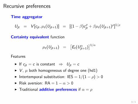
Recursive preferences

Time aggregator

Ujt = V [cjt , µt(Ujt+1)] = [(1− β)cρjt + βµt(Ujt+1)ρ]1/ρ

Certainty equivalent function

µt(Ujt+1) =[Et(U

αjt+1)

]1/α

Features

I If cjt = c is constant ⇒ Ujt = c

I V , µ both homogeneous of degree one (hd1)

I Intertemporal substitution: IES = 1/(1− ρ) > 0

I Risk aversion: RA = 1− α > 0

I Traditional additive preferences if α = ρ

3 / 1

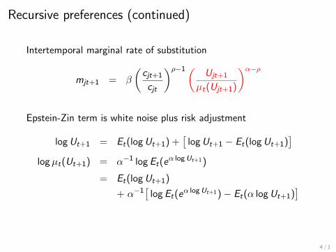
Recursive preferences (continued)

Intertemporal marginal rate of substitution

mjt+1 = β

(cjt+1

cjt

)ρ−1 ( Ujt+1

µt(Ujt+1)

)α−ρ

Epstein-Zin term is white noise plus risk adjustment

logUt+1 = Et(logUt+1) +[

logUt+1 − Et(logUt+1)]

logµt(Ut+1) = α−1 log Et(eα log Ut+1)

= Et(logUt+1)

+ α−1[

log Et(eα log Ut+1)− Et(α logUt+1)

]

4 / 1

Two-country model

5 / 1

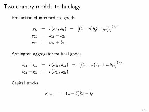
Two-country model: technology

Production of intermediate goods

yjt = f (kjt , zjt) =[(1− η)kνjt + ηzνjt

]1/ν

y1t = a1t + a2t

y2t = b1t + b2t

Armington aggregator for final goods

c1t + i1t = h(a1t , b1t) =[(1− ω)aσ1t + ωbσ1t

]1/σ

c2t + i2t = h(b2t , a2t)

Capital stocks

kjt+1 = (1− δ)kjt + ijt

6 / 1

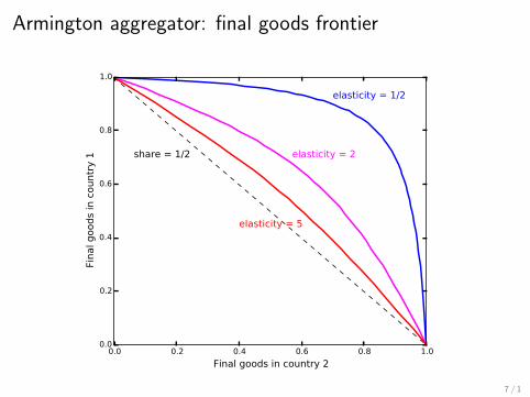
Armington aggregator: final goods frontier

0.0 0.2 0.4 0.6 0.8 1.0

Final goods in country 2

0.0

0.2

0.4

0.6

0.8

1.0

Final goods

in c

ountr

y 1 share = 1/2

elasticity = 1/2

elasticity = 2

elasticity = 5

7 / 1

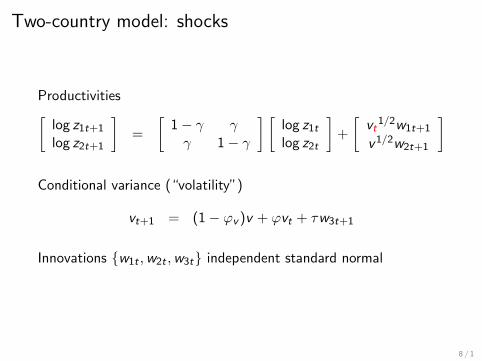
Two-country model: shocks

Productivities[log z1t+1

log z2t+1

]=

[1− γ γγ 1− γ

] [log z1t

log z2t

]+

[vt

1/2w1t+1

v1/2w2t+1

]

Conditional variance (“volatility”)

vt+1 = (1− ϕv )v + ϕvt + τw3t+1

Innovations {w1t ,w2t ,w3t} independent standard normal

8 / 1

Pareto problem

9 / 1

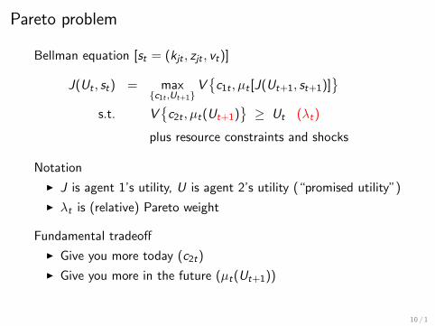
Pareto problem

Bellman equation [st = (kjt , zjt , vt)]

J(Ut , st) = max{c1t ,Ut+1}

V{c1t , µt [J(Ut+1, st+1)]

}s.t. V

{c2t , µt(Ut+1)

}≥ Ut (λt)

plus resource constraints and shocks

Notation

I J is agent 1’s utility, U is agent 2’s utility (“promised utility”)

I λt is (relative) Pareto weight

Fundamental tradeoff

I Give you more today (c2t)

I Give you more in the future (µt(Ut+1))

10 / 1

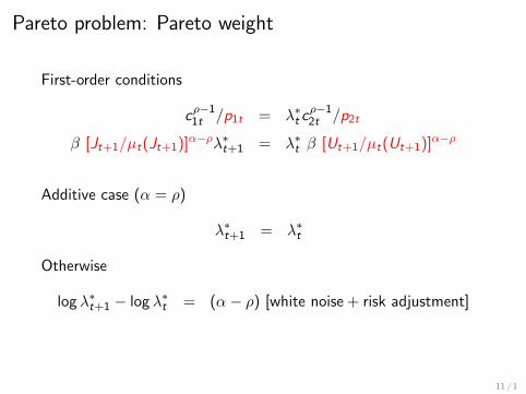
Pareto problem: Pareto weight

First-order conditions

cρ−11t /p1t = λ∗t c

ρ−12t /p2t

β [Jt+1/µt(Jt+1)]α−ρλ∗t+1 = λ∗t β [Ut+1/µt(Ut+1)]α−ρ

Additive case (α = ρ)

λ∗t+1 = λ∗t

Otherwise

log λ∗t+1 − log λ∗t = (α− ρ) [white noise + risk adjustment]

11 / 1

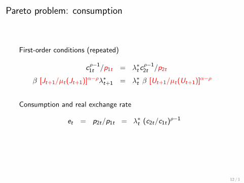
Pareto problem: consumption

First-order conditions (repeated)

cρ−11t /p1t = λ∗t c

ρ−12t /p2t

β [Jt+1/µt(Jt+1)]α−ρλ∗t+1 = λ∗t β [Ut+1/µt(Ut+1)]α−ρ

Consumption and real exchange rate

et = p2t/p1t = λ∗t (c2t/c1t)ρ−1

12 / 1

Numerical examples: exchange economy

13 / 1

Computation

Method adapted from Collin-Dufresne, Johannes, and Lochstoer

I Global projection method

I Implemented in Julia for speed

I State changed from Ut to sat = a1t/y1t or λ∗t

P2C2E

14 / 1

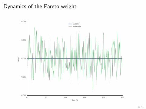
Dynamics of the Pareto weight

0 50 100 150 200 250

time (t)

0.010

0.005

0.000

0.005

0.010

∆lo

gλ∗

AdditiveRecursive

15 / 1

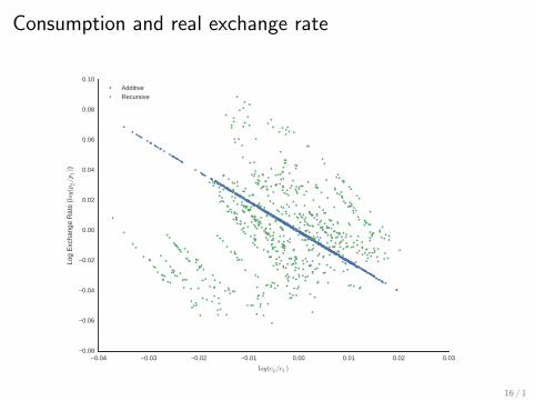
Consumption and real exchange rate

0.04 0.03 0.02 0.01 0.00 0.01 0.02 0.03

log(c2/c1 )

0.08

0.06

0.04

0.02

0.00

0.02

0.04

0.06

0.08

0.10

Log 

Exc

hang

e R

ate 

(log

(p2/p

1))

AdditiveRecursive

16 / 1

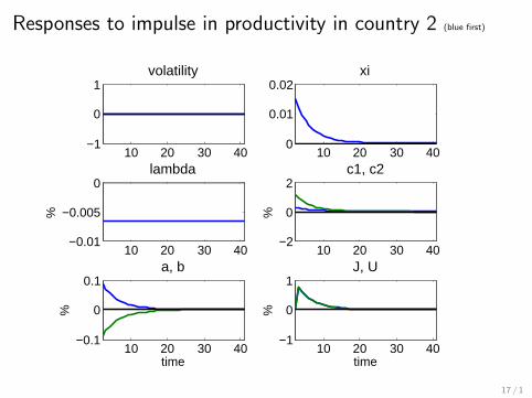
Responses to impulse in productivity in country 2 (blue first)

10 20 30 40−1

0

1volatility

10 20 30 400

0.01

0.02xi

10 20 30 40−0.01

−0.005

0lambda

%

10 20 30 40−2

0

2c1, c2

%

10 20 30 40−0.1

0

0.1a, b

%

time10 20 30 40

−1

0

1J, U

%

time

Student Version of MATLAB

17 / 1

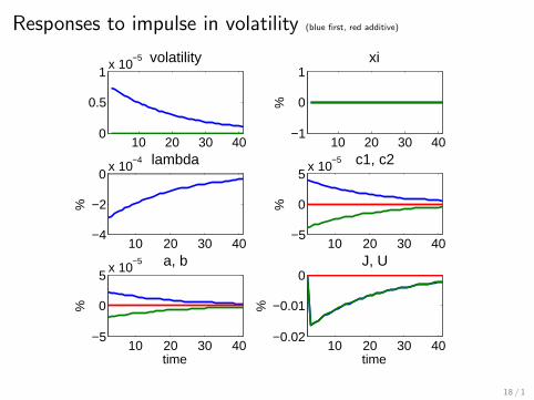
Responses to impulse in volatility (blue first, red additive)

10 20 30 400

0.5

1x 10

−5 volatility

10 20 30 40−1

0

1xi

%

10 20 30 40−4

−2

0x 10

−4 lambda

%

10 20 30 40−5

0

5x 10

−5 c1, c2

%

10 20 30 40−5

0

5x 10

−5 a, b

%

time10 20 30 40

−0.02

−0.01

0J, U

%

time

Student Version of MATLAB

18 / 1

Numerical examples: production economy

19 / 1

Investment and volatility

[We’re working on this, harder than we thought]

20 / 1

Stability

21 / 1

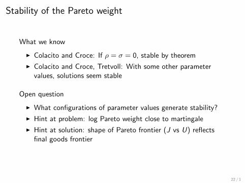
Stability of the Pareto weight

What we know

I Colacito and Croce: If ρ = σ = 0, stable by theorem

I Colacito and Croce, Tretvoll: With some other parametervalues, solutions seem stable

Open question

I What configurations of parameter values generate stability?

I Hint at problem: log Pareto weight close to martingale

I Hint at solution: shape of Pareto frontier (J vs U) reflectsfinal goods frontier

22 / 1

Last thought

What would you do with this material?

23 / 1