Embed Size (px)
Citation preview

HAL Id: tel-01075751https://hal.archives-ouvertes.fr/tel-01075751
Submitted on 20 Oct 2014
HAL is a multi-disciplinary open accessarchive for the deposit and dissemination of sci-entific research documents, whether they are pub-lished or not. The documents may come fromteaching and research institutions in France orabroad, or from public or private research centers.
L’archive ouverte pluridisciplinaire HAL, estdestinée au dépôt et à la diffusion de documentsscientifiques de niveau recherche, publiés ou non,émanant des établissements d’enseignement et derecherche français ou étrangers, des laboratoirespublics ou privés.
Risk Assesment and Intrusion Detection for AirborneNetworks
Silvia Gil-Casals
To cite this version:Silvia Gil-Casals. Risk Assesment and Intrusion Detection for Airborne Networks. Networking andInternet Architecture [cs.NI]. INSA Toulouse, 2014. English. �tel-01075751�

THÈSETHÈSEEn vue de l’obtention du
DOCTORAT DE L’UNIVERSITÉ DE TOULOUSEDélivré par : l’Institut National des Sciences Appliquées de Toulouse (INSA de Toulouse)
Présentée et soutenue le 21 juillet 2014 par :Silvia Gil Casals
Risk Assesment and Intrusion Detection for Airborne Networks
JURYVincent Nicomette Président du JuryIsabelle Chrisment RapporteurDamien Magoni RapporteurKrishna Sampigethaya ExaminateurPhilippe Owezarski Directeur de thèseGilles Descargues Encadrant de thèse
École doctorale et spécialité :MITT : Domaine STIC : Réseaux, Télécoms, Systèmes et Architecture
Unité de Recherche :Laboratoire d’Analyse et d’Architecture des Systèmes (UPR 8001)
Directeur(s) de Thèse :Philippe Owezarski et Gilles Descargues
Rapporteurs :Isabelle Chrisment et Damien Magoni


RISK ASSESSMENT AND INTRUSION
DETECTION FOR AIRBORNE NETWORKS
ABSTRACT
Aeronautics is actually facing a confluence of events: connectivity of aircraft is gradually
increasing in order to ease the air traffic management and aircraft fleet maintainability, and to
offer new services to passengers while reducing costs. The core avionics functions are thus
linked to what we call the Open World, i.e. the non-critical network of an aircraft as well as the
air traffic services on the ground. Such recent evolutions could be an open door to cyber-attacks
as their complexity keeps growing. However, even if security standards are still under
construction, aeronautical certification authorities already require that aircraft manufacturers
identify risks and ensure aircraft will remain in a safe and secure state even under threat
conditions.
To answer this industrial problematic, this thesis first proposes a simple semi-quantitative risk
assessment framework to identify threats, assets and vulnerabilities, and then rank risk levels
according to threat scenario safety impact on the aircraft and their potential likelihood by using
adjustable attribute tables. Then, in order to ensure the aircraft performs securely and safely
all along its life-cycle, our second contribution consists in a generic and autonomous network
monitoring function for intrusion detection based on Machine Learning algorithms. Different
building block options to compose this monitoring function are proposed such as: two ways of
modeling the network traffic through characteristic attributes, two Machine Learning
techniques for anomaly detection: a supervised one based on the One Class Support Vector
Machine algorithm requiring a prior training phase and an unsupervised one based on sub-
space clustering. Since a very common issue in anomaly detection techniques is the presence
of false alarms, we prone the use of the Local Outlier Factor (a density indicator) to set a
threshold in order to distinguish real anomalies from false positives.
This thesis summarizes the work performed under the CIFRE (Convention Industrielle de Formation par
la Recherche) fellowship between THALES Avionics and the CNRS-LAAS at Toulouse, France.
Keywords: airworthiness security, risk assessment, process, intrusion/anomaly detection,
Machine Learning


ANALYSE DE RISQUE ET DETECTION
D'INTRUSIONS POUR LES RESEAUX
AVIONIQUES
RÉSUMÉ
L'aéronautique connaît de nos jours une confluence d'événements: la connectivité bord-sol et au sein
même de l’avion ne cesse d'augmenter afin, entre autres, de faciliter le contrôle du trafic aérien et la
maintenabilité des flottes d’avions, offrir de nouveaux services pour les passagers tout en réduisant les
coûts. Les fonctions avioniques se voient donc reliées à ce qu’on appelle le Monde Ouvert, c’est-à-dire
le réseau non critique de l’avion ainsi qu’aux services de contrôle aérien au sol. Ces récentes évolutions
pourraient constituer une porte ouverte pour les cyber-attaques dont la complexité ne cesse de croître
également. Cependant, même si les standards de sécurité aéronautique sont encore en cours d'écriture,
les autorités de certification aéronautiques demandent déjà aux avionneurs d'identifier les risques et
assurer que l'avion pourra opérer de façon sûre même en cas d'attaque.
Pour répondre à cette problématique industrielle, cette thèse propose une méthode simple d'analyse
de risque semi-quantitative pour identifier les menaces, les biens à protéger, les vulnérabilités et classer
les différents niveaux de risque selon leur impact sur la sûreté de vol et de la potentielle vraisemblance
de l’attaque en utilisant une série de tables de critères d’évaluation ajustables. Ensuite, afin d'assurer
que l'avion opère de façon sûre et en sécurité tout au long de son cycle de vie, notre deuxième
contribution consiste en une fonction générique et autonome d'audit du réseau pour la détection
d'intrusions basée sur des techniques de Machine Learning. Différentes options sont proposées afin de
constituer les briques de cette fonction d’audit, notamment : deux façons de modéliser le trafic au
travers d’attributs descriptifs de ses caractéristiques, deux techniques de Machine Learning pour la
détection d’anomalies : l’une supervisée basée sur l’algorithme One Class Support Vector Machine et
qui donc requiert une phase d’apprentissage, et l’autre, non supervisée basée sur le clustering de sous-
espace. Puisque le problème récurrent pour les techniques de détection d’anomalies est la présence de
fausses alertes, nous prônons l’utilisation du Local Outlier Factor (un indicateur de densité) afin d’établir
un seuil pour distinguer les anomalies réelles des fausses alertes.
Ce mémoire rend compte du travail effectué dans le cadre d’une convention CIFRE (Convention
Industrielle de Formation par la Recherche) entre THALES Avionics et le CNRS-LAAS de Toulouse.
Mots-clé: sécurité des réseaux avioniques, analyse de risque, processus, détection
d’anomalies/d’intrusions, Machine Learning

To my parents,

ACKNOWLEDGEMENTS
This report summarizes the research work of this 3-year PhD made under CIFRE (Conventions
Industrielles de Formation par la REcherche) convention fellowship financed by the ANRT (Association
Nationale de la Recherche et de la Technologie), between the Laboratoire d’Analyses et Systèmes (LAAS)
of the Centre National de Recherche Scientifique (CNRS) and THALES Avionics Toulouse. I would like to
thank the director of the LAAS, Jean Arlat, as well as the director of the Services et Architectures pour
les Réseaux Avancés (SARA) research group, Khalil DRIRA. I am also grateful to the whole CCS (Centre de
Compétences Système) department of THALES Avionics.
I would like to thank Philippe Owezarski, my PhD director and researcher at the SARA
department of the LAAS-CNRS and Gilles Descargues, my industrial advisor and systems engineer at CCS
department of THALES Avionics for giving me the opportunity to work on this subject. Sincere thanks to
Stéphane PLICHON and Christian SANNINO from THALES Avionics that reviewed this report.
I am very thankful to the other members of my committee for honoring me by their presence at my PhD defense:
Isabelle Chrisment (LORIA) Damien Magoni (LABRI) Krishna Sampigethaya (University of Washington) Vincent Nicomette (INSA, LAAS-CNRS)
I would like to express my gratitude to Johan, Pedro, Guillaume K., Guillaume D., Cédric, Denis,
Lionel, Codé, Mark, Anthony, Ghada, Maxence… and all my other colleagues from the LAAS for their
help, moral support and the laughs that made research easier, as well as all my THALES Avionics
colleagues: Sara, Sylvie, Stéphanie, Valérie, Céline, Anne, Sandrine, Olivier, Didier, JLo, Stéphane, Michel
C., Michel M., Michel H., Fabien, Gabrielle, Cédric, Nicolas, David and the interns for their kindness (I
apologize in advance if I forgot your name, but I am already stressed and I can’t think clearly! ). Also,
thanks to all my friends: the musicians, the dancers, the geeks, Aude & Damien, and the others for the
good times, and especially to Vincent PRIVAT for his help, encouragement and support. To you all:
THANK YOU!
Last but not least, I would like to thank my parents for their unconditional love and support in
all and every one of my projects (even the craziest ones), I owe you so much!


CONTENTS
CHAPTER 1: INTRODUCTION .......................................................................................... 1
1.1. MOTIVATION AND PROBLEM STATEMENT ........................................................................................................ 1
1.2. EMERGING CHALLENGES AND CONTRIBUTIONS ................................................................................................. 3
1.2.1. Emerging Challenges in Terms of Process ..................................................................................... 3
1.2.2. Process and Risk Assessment Contributions.................................................................................. 3
1.2.3. Emerging Challenges in Terms of Intrusion Detection Systems .................................................... 4
1.2.4. Audit Function for Airborne Networks Security Monitoring .......................................................... 4
1.3. THESIS STRUCTURE ..................................................................................................................................... 5
CHAPTER 2: THE AERONAUTICAL CONTEXT .................................................................... 7
2.1. SECURITY INCIDENTS SUMMARY .................................................................................................................... 7
2.1.1. Attacks in Aviation ........................................................................................................................ 7 2.1.1.1. Attacks on aviation ground facilities ........................................................................................................ 7 2.1.1.2. Aviation incidents due to misuse .............................................................................................................. 8 2.1.1.3. What about aircraft hijacking? ................................................................................................................. 8 2.1.1.4. Summary .................................................................................................................................................. 9
2.1.2. Attacks in Other Domains ............................................................................................................. 9 2.1.2.1. Car hijacking ............................................................................................................................................. 9 2.1.2.2. Stuxnet: attacking critical facilities ........................................................................................................... 9
2.2. THE EVOLUTION OF AIRBORNE SYSTEMS ....................................................................................................... 10
2.2.1. Recent and Upcoming Innovations ............................................................................................. 11 2.2.1.1. From federated to integrated architectures........................................................................................... 11 2.2.1.2. From A429 to ADN (Aircraft Data Networks) .......................................................................................... 12 2.2.1.3. Software distribution and modification .................................................................................................. 13 2.2.1.4. COTS introduction and use of passenger owned devices ....................................................................... 13 2.2.1.5. From voice to digital messages exchange .............................................................................................. 14 2.2.1.6. Networks interoperability and infrastructure sharing with NextGen ..................................................... 14 2.2.1.7. The E-enabled aircraft ............................................................................................................................ 16
2.2.2. Hazards Associated to Complex and Inter-Connected Architectures .......................................... 16 2.2.2.1. Countering safety issues in aeronautics ................................................................................................. 17 2.2.2.2. Failures prevention ................................................................................................................................. 18 2.2.2.3. Errors prevention ................................................................................................................................... 18 2.2.2.4. Misuse prevention .................................................................................................................................. 18 2.2.2.5. Countering security issues in the aeronautics ........................................................................................ 18
2.3. EMERGING AERONAUTICAL SECURITY CHALLENGES ......................................................................................... 19
2.3.1. Potential Threats ......................................................................................................................... 19
2.3.2. On-board security ....................................................................................................................... 20
2.3.3. Air-ground security ..................................................................................................................... 20
2.4. CHAPTER SUMMARY .................................................................................................................................. 21

CHAPTER 3: RISK ASSESSMENT & SECURITY PROCESS ................................................... 23
3.1. RISK ASSESSMENT METHODOLOGY .............................................................................................................. 23
3.1.1. Basic Security Risk Assessment Concepts and Definitions ........................................................... 23
3.1.2. State of the Art on Risk Assessment Methods............................................................................. 26
3.2. RISK ASSESSMENT FRAMEWORK DESCRIPTION ............................................................................................... 30
3.2.1. Step 1: Context Establishment .................................................................................................... 31
3.2.2. Step 2: Preliminary Risk Assessment (top-down approach) ........................................................ 31
3.2.3. Step 3: Vulnerability Assessment (bottom-up approach)............................................................ 33
3.2.4. Step 4: Risk Estimation ................................................................................................................ 33
3.2.5. Step 5: Security Requirements .................................................................................................... 36
3.2.6. Step 6: Risk Treatment ................................................................................................................ 36
3.3. SECURITY PROCESS ................................................................................................................................... 37
3.4. CHAPTER SUMMARY ................................................................................................................................. 38
CHAPTER 4: THEORY ON SECURITY AUDIT .................................................................... 39
4.1. STATE OF THE ART ON INTRUSION DETECTION SYSTEMS ................................................................................... 39
4.1.1. Misuse vs. anomaly detection, behavioral analysis justification ................................................ 39
4.1.2. Related work concerning security monitoring in airborne networks .......................................... 41
4.1.3. Machine Learning algorithms and related anomaly detection techniques ................................. 41 4.1.3.1. Supervised Learning ............................................................................................................................... 42 4.1.3.2. Unsupervised Learning ........................................................................................................................... 45 4.1.3.3. One Class Classification Methods ........................................................................................................... 48
4.1.4. Feature selection for network traffic characterization ............................................................... 49 4.1.4.1. Most common attributes used to describe network traffic in literature ................................................ 49 4.1.4.2. Importance of scaling ............................................................................................................................. 51 4.1.4.3. Feature selection and dimensionality reduction .................................................................................... 51
4.2. THEORY ON SUPPORT VECTOR MACHINES AND ONE CLASS SVM ...................................................................... 52
4.2.1. Original SVM algorithm .............................................................................................................. 52 4.2.1.1. The optimization problem ...................................................................................................................... 52 4.2.1.2. Quadratic programming and Support vectors ........................................................................................ 54 4.2.1.3. Slack variables ........................................................................................................................................ 55 4.2.1.4. Kernel trick for non-linearly separable problems ................................................................................... 55
4.2.2. One Class SVM ............................................................................................................................ 57 4.2.2.1. OCSVM.................................................................................................................................................... 57 4.2.2.2. Support Vector Data Description (SVDD) ............................................................................................... 57 4.2.2.3. Graphical interpretation and comparison of SVDD and OCSVM ............................................................ 58
4.3. CHAPTER SUMMARY ................................................................................................................................. 59
CHAPTER 5: AIRBORNE NETWORKS’ INTRUSION DETECTION FUNCTION ....................... 61
5.1. THE SECURITY MONITORING FUNCTION FRAMEWORK ..................................................................................... 61
5.1.1. Step 1: Data Acquisition .............................................................................................................. 62
5.1.2. Step 2: Data Preprocessing ......................................................................................................... 63
5.1.3. Step 3: Sample Classification ...................................................................................................... 63
5.1.4. Step 4: Post-Treatment ............................................................................................................... 64
5.2. CONTEXT OF TRAFFIC CAPTURE .................................................................................................................... 65
5.2.1. Architecture description .............................................................................................................. 65
5.2.2. Traffic capture ............................................................................................................................. 67
5.2.3. Main characteristics of the “normal” traffic ............................................................................... 67
5.2.4. Attacks of the Evaluation Dataset .............................................................................................. 68 5.2.4.1. Probe / Scan ........................................................................................................................................... 68

5.2.4.2. Flooding .................................................................................................................................................. 70 5.2.4.3. Packet Replay ......................................................................................................................................... 71
5.2.5. IDS Performance Evaluation Metrics .......................................................................................... 71
5.3. FIRST ATTRIBUTE PROPOSAL FOR STEP 2 ....................................................................................................... 73
5.3.1. Attributes Set #1 description ....................................................................................................... 73
5.3.2. Feature Influence ........................................................................................................................ 75
5.4. UNSUPERVISED LEARNING PROPOSAL FOR STEP 3: SUB-SPACE CLUSTERING......................................................... 76
5.4.1. The Origins: Simple Clustering Results ........................................................................................ 76
5.4.2. Sub-Space Clustering ................................................................................................................... 77
5.4.3. Reducing False Positives using the Local Outlier Factor (LOF) .................................................... 79
5.4.4. Detection Results With and Without the LOF Threshold and Discussion ................................... 80
5.5. SUPERVISED PROPOSAL FOR STEP 3: ONE CLASS SVM..................................................................................... 82
5.5.1. Reminder of OCSVM parameters ................................................................................................ 82
5.5.2. OCSVM Calibration (Grid-search Results) ................................................................................... 82
5.5.3. Influence of Training Data Set Volume on OCSVM ..................................................................... 86
5.5.4. Processing Time .......................................................................................................................... 87
5.6. INFLUENCE OF THE OBSERVATION WINDOW SIZE ............................................................................................ 88
5.6.1. Initial Hypothesis ......................................................................................................................... 88
5.6.2. Hypothesis Refutation ................................................................................................................. 90
5.7. SECOND ATTRIBUTE PROPOSAL FOR STEP 2 ................................................................................................... 92
5.7.1. Justification ................................................................................................................................. 92
5.7.2. Attributes Set #2 description ....................................................................................................... 93
5.7.3. To go further ............................................................................................................................... 94
5.8. CHAPTER SUMMARY .................................................................................................................................. 95
CHAPTER 6: CONCLUSION ............................................................................................ 97
6.1. CONTRIBUTIONS ....................................................................................................................................... 97
6.1.1. Risk Assessment Methodology and Security Process .................................................................. 97
6.1.2. Airborne Networks’ Intrusion Detection Function Framework ................................................... 98
6.2. PERSPECTIVES .......................................................................................................................................... 99
6.2.1. Hints of Improvement for the Security Monitoring Function ...................................................... 99 6.2.1.1. Normal Behavior for each Flight Phase .................................................................................................. 99 6.2.1.2. Redundant and Dissimilar Architecture ................................................................................................ 100 6.2.1.3. Coupling with Flight Warning Systems ................................................................................................. 101
6.2.2. Open Questions ......................................................................................................................... 101
ACRONYMS.................................................................................................................... 105
REFERENCES .................................................................................................................. 109
ADN (AIRCRAFT DATA NETWORKS) ................................................................................ 121
A1.1. BEFORE ADN ........................................................................................................................................ 121
A1.2. BASIC AFDX NEEDS ................................................................................................................................ 121
A1.3. SOME AFDX CHARACTERISTICS ................................................................................................................. 122
TRIPLE V-CYCLE .............................................................................................................. 125
A2.1. THE DEVELOPMENT PROCESS .................................................................................................................... 125
A2.2. THE SAFETY PROCESS .............................................................................................................................. 126
A2.3. THE SECURITY FOR SAFETY PROCESS ........................................................................................................... 127
A2.4. THE TRIPLE-V CYCLE PROCESS GRAPH ........................................................................................................ 128


1
1. CHAPTER 1
INTRODUCTION
1.1. MOTIVATION AND PROBLEM STATEMENT
Aeronautics is actually facing a confluence of events. On the one hand, connectivity of aircraft is
gradually growing which leads to the design of new systems and architectures, while there is still a lack
of industrial process framework to deal with security. On the other hand, cyber-attacks keep increasing
too and demonstrations of vulnerabilities are made public. Meanwhile, the aeronautical standards
dealing with airborne security have not been issued yet. However, in recently released airplanes, the
EASA1 and the FAA2, respectively EU and US aeronautical certification authorities, have addressed
Certification Review Items (CRIs) and Special Conditions3 (SCs) to aircraft manufacturers with additional
aspects to be taken into consideration concerning the protection against malicious acts. Generally, it is
required that:
1. Aircraft systems and networks’ security protection is ensured from unauthorized sources access, since their corruption by an inadvertent or intentional attack would impair safety of flight.
2. Security threats to the aircraft (including those possibly caused by maintenance activity or any unprotected connecting equipment/devices) are identified, assessed and risk mitigation strategies are implemented to protect the aircraft systems from all adverse impacts on safety of flight.
3. Continued airworthiness of the aircraft is maintained, including all post Type Certificate modifications, which have an impact on the approved network security safeguards, by establishing appropriate procedures.
Answering to CRIs’ and SCs’ requests is all the more compulsory as it conditions the Type Certificate4 delivery, which is mandatory for an airplane to fly. As a matter of fact, there are new airworthiness security standards being written that will harden the obligation of dealing with security. These CRIs and SCs are the initial industrial problematic that has inspired this thesis on airworthiness5 security. It focuses mainly on two subjects that are:
1 European Aviation Safety Agency 2 Federal Aviation Administration 3 An example of Special Condition can be seen at: https://www.federalregister.gov/articles/2013/11/18/2013-27343/special-
conditions-boeing-model-777-200--300-and--300er-series-airplanes-aircraft-electronic-system 4 Certifies the aircraft suitability for safe flight, i.e. that a given aircraft model has been manufactured according to a previously
approved design in compliance with airworthiness requirements. 5 Aircraft trustworhiness of flight

2
Process aspect. The definition of a risk assessment methodology both compliant with the future security standards and compatible with the overall industrial design process to answer point n°2.
Technical aspect. The design and validation of a network monitoring function based on Machine Learning for intrusion detection and characterization of anomalies potentially caused by cyber-threats to ensure that continued airworthiness is maintained (point n° 3).
Continued Airworthiness. During design, some aspects cannot be mastered such as the evolution of
threats, the reevaluation of COTS’ vulnerabilities and the correct functioning of the security
countermeasures towards these threats. The concept of continued airworthiness, common to safety
and security processes, consists in certifying that the system itself and its countermeasures perform
safely and securely all along the aircraft operational life-time. It is done among others by providing a
planning to certification authorities of the periodical activities of technology watch in terms of system
vulnerabilities, new attacks, testing the system towards these new attacks for instance, managing the
eventual changes, etc. The guidance for airworthiness continuity maintenance will be provided in the
future standard ED-204 : “Airworthiness Security Instructions for Continued Airworthiness”. According
to us, one of the pillars of the continued airworthiness is the continuous security monitoring of airborne
systems and networks, in order to evaluate existing countermeasures effectiveness such as firewalls but
also to keep logs on occurring attacks in order to better understand them and feed risk assessment
methodologies on attack probabilities of occurrence.
The fundamental axes addressed in this thesis are the following (fig. 1.1): based on the future airworthiness security process activities and on the security standards, our first contribution has been a risk assessment methodology applicable to airborne networks and systems. Our second contribution has consisted in using Machine Learning techniques to build an intrusion detection system dedicated to airborne networks.
Figure 1.1. – Thematic axes of this thesis

3
1.2. EMERGING CHALLENGES AND CONTRIBUTIONS
1.2.1. EMERGING CHALLENGES IN TERMS OF PROCESS
In heavy industry of complex systems such as the aeronautics, processes are crucial to ensure the
correct interfacing and synchronization between teams working on different segments of an aircraft, at
different life-cycle steps of the development (design, implementation, verification and validation) and
transversal activities such as quality control, safety process or certification. The concept of airworthiness
security is a very brand new domain, it aims at assessing potential misuse acts or intentional intrusions
that could lead to the loss of airworthiness, i.e. hazardous events on the aircraft. The term must not be
mixed up with safety that, contrary to security, assesses accidental system failures that could originate
the loss of airworthiness. Safety process is well-established and well integrated within the overall
development process and has proved its efficiency for more than 50 years. Nevertheless, the security
process is actually very poor or even non-existent in the aeronautics industry. There are three standards
under construction by committees from the EUROCAE (EU) and the RTCA (US) namely the DO-326A/ED-
202 [1] that provides the security process guidelines, the DO-YY3/ED-203 [2] that will give the methods
and tools to achieve the process objectives (for instance: risk assessment methodologies) and the
DOYY4/ED-204 [3] that lists the instructions for continued airworthiness (for instance: software copying,
storage and distribution, training, access control methods, digital certificates, etc.). However, only the
ED-202A has been released and the rest are still not applicable. The emergence of this new activity
arises many questions: who should be in charge of airborne security at the very beginning: security
experts or airborne systems experts? How should this activity be integrated to the overall development
process? Should it be lead at an early step of development (which would imply having systems architects
aware on unsecure designs) or afterwards (implying costly changes to the architecture)? Should safety
and security processes be merged and how? This is a very long reflection process implying a lot of
stakeholders that will not be solved in this thesis!
1.2.2. PROCESS AND RISK ASSESSMENT CONTRIBUTIONS
What we did at the beginning of this thesis is defining the main activities for the future security process
by deducing them from the standards under construction and taking inspiration on how safety
standards have been tailored within the company. Part of this work was performed in the context of
SEISES6 project that lead to the definition of a triple V-cycle showing the activities, output documents
and interactions between the security, safety and development processes that we present here as our
first industrial contribution.
6 Systèmes Embarqués Informatisés, Sûrs et Sécurisés (translation: computerized safe and secure embedded systems) is an
Aerospace Valley collaborative project between Airbus, Rockwell Collins, Astrium, Serma Technologies, Apsys, EADS, Onera, DGA, Thales Avionics, LSTI, LAAS-CNRS for the definition and linking of safety and security processes’ activities for embedded systems.

4
The other process-related task we were given consisted in the definition of a risk assessment framework
to answer CRI’s requirement number 2, that can be integrated at an early step of development (i.e.
before any implementation). To do so, the method consists in identifying the assets to be protected and
the potential security threats to the aircraft and assessing risk to deploy adapted mitigation strategies.
The risk acceptability of a given threat scenario is measured through the combination of its safety impact
on the aircraft and its likelihood. The likelihood itself is determined by the combination of two factors:
the attacker capability and the asset exposure each measured on a semi-quantitative manner by using
tables with adaptable characterization attributes.
The work concerning the risk assessment methodology framework “Risk Assessment for Airworthiness
Security” has been published on the proceedings of the 31st International Conference on Computer
Safety, Reliability and Security (SafeComp) held in Magdeburg, Germany on 24-28 September 2012 [4].
1.2.3. EMERGING CHALLENGES IN TERMS OF INTRUSION DETECTION SYSTEMS
If a security breach exploitation is detected on board, it is possible that actions are taken to reduce its
impact (e.g. having the flight crew disengaging the autopilot function to take manual control) or to
prevent its occurrence (e.g. automatically updating filters with new detected threats signatures). Thus,
the detection of intrusions should be fast enough to be made on real time, accurate enough not to miss
any attempt and not to provide false alarms. Indeed, false alarms could be as dangerous as the attack
itself because it could mislead flight crew or block/disable critical flows or applications. Another issue to
be considered is the aircraft lifetime (usually around 30 years), to reduce maintenance costs, the ideal
would be to have long-term security solutions [5], i.e. an autonomous system to detect the attacks no
matter the operational phase of the aircraft.
The problem of most commercial Intrusion Detection Systems (IDS) is that their effectiveness relies
exclusively on the exhaustiveness of their attack signatures databases. These systems dedicated to
attack-signature pattern matching are referred to as signature-based or misuse techniques, and as such,
they fail at detecting novel attacks. Also, they must be very often updated with new signatures. On the
other hand, other techniques rather focused on training a system uniquely on normal events to detect
any deviation from usual behavior, called Anomaly Detection Systems (ADS), are under research. It is
very common to use Machine Learning techniques for such tasks. But tests have proved that the latter
are tricky to parameterize and produce an important amount of false alarms and/or undetected attacks.
Given the criticality of the avionics domain, it is necessary to optimize the detection accuracy, but still
ignoring the nature of the attacks that could occur in such an environment unless by extrapolating from
the IT domain.
1.2.4. AUDIT FUNCTION FOR AIRBORNE NETWORKS SECURITY MONITORING
In this thesis, we propose a framework for a generic and autonomous network security monitoring
function that continuously captures packets from the network, eventually samples them and extracts
traffic characteristics to feed a Machine Learning algorithm that determines whether the samples are
normal (i.e. belong to the majority of observed classes in a prior training step) or anomalous (i.e. the

5
behavior in the sample differs in some way from what has been learned by the algorithm). This
framework is composed of four steps:
1. Data acquisition: consists in network traffic capture and packet timestamping
2. Pre-processing to build descriptive attributes among the data and pre-process them (scaling, redundancy elimination)
3. Sample classification: the Machine Learning algorithm is fed with the data produced in step 2 to determine the label of the sample (i.e. normal or anomalous)
4. Post-processing of step 3 results to reduce the amount of false positives and get the characteristics of the attack
What is being feared in the embedded network example we have taken for this thesis are:
Network scans and Denial of Service (DoS) attacks that could be originated from the Open
World, also called Ethernet Open Network (EON) to gather information or try to access the
Aircraft Data Network (ADN), i.e. the critical core avionics network. Note that EON and ADN are
connected through a gateway.
The presence of maliciously crafted packets in the ADN network itself.
To detect these attacks, we propose two different ways of modeling each type of network traffic
through attribute sets at step 2: one based of observation window slices of a given width ΔT for scans
and DoS on the EON side, and another one that is packet-based and takes advantage of the ADN traffic
determinism for individual anomalous packets.
Then, for step 3 we propose two different classification techniques: a supervised one based on the One
Class Support Vector Machines (OCSVM) algorithm that requires training on exclusively normal traffic
and an unsupervised one based on sub-space clustering that does not require a training phase.
To make sure the detection is accurate and thus avoid false positives, we propose to compute the Local
Outlier Factor (a density-based coefficient to identify local outliers by comparison to the neighborhood
density) in the post-treatment phase, in order to distinguish true anomalies from false alarms. We also
propose a way to determine the most significant attributes that better distinguish the anomaly from the
normal traffic.
The performances of the different possible building blocks proposed respectively for steps 2 and 3 are
measured and the influence of their parameters analyzed. We then provide hints for the improvement
of such an embedded monitoring function.
Our first tests for the audit function “Generic and autonomous system for airborne networks cyber-
threat detection” were published on the proceedings of the 32nd Digital Avionics Systems Conference
(DASC) held in Syracuse, NY on 4-10 October 2013 [6].
1.3. THESIS STRUCTURE
The rest of the dissertation is composed as following:
CHAPTER 2 depicts the industrial context of this thesis with: some minor security incidents that
have already occurred in the aviation environment, the actual and upcoming aeronautical

6
innovations that could potentially introduce vulnerabilities to cyber-security threats, and some
solutions that are actually under research to prevent or reduce such security issues.
After defining some basic security assessment terms and making a brief state of the art on actual
security risk management methods, CHAPTER 3 describes the different steps of our risk assessment
methodology framework proposal to answer simply and systematically to CRIs’ requirements. We
also present our first recommendations in terms of security activities to be integrated in the future
airworthiness security process as well as the interactions with the safety and the development
processes.
CHAPTER 4 draws a state of the art on intrusion detection systems, and especially on supervised
and unsupervised Machine Learning techniques, as well as a theoretical insight into the techniques
we are using in our intrusion detection system: clustering algorithms and Support Vector Machines
(SVM) and more concretely the One Class SVM algorithm.
First, CHAPTER 5 provides the generic framework for an autonomous security monitoring function.
Then, it describes the concrete context of network traffic capture as well as the attacks that are
aimed to be detected and our evaluation approach. After, we propose different implementation
building-blocks possibilities: two different ways of modeling the network traffic through descriptive
attributes, and two different Machine Learning approaches: supervised and unsupervised,
respectively One Class SVM and sub-space clustering. The effectiveness and efficiency evaluation
are provided to constitute a proof of concept. We also propose a post-treatment step to get rid of
false positives and deduce the characteristics of the attack.
Finally, CHAPTER 6 concludes the dissertation by summarizing the main contributions, their
advantages and weaknesses. It also provides some improvement hints for more accurate attack
detection as well as perspectives on how to integrate safety and security alarms to correlate
potentially linked effects.

7
2. 2.
CHAPTER 2
THE AERONAUTICAL CONTEXT
In security it is more a matter of when than a matter of if. In this chapter, we describe the industrial
context in which this PhD has taken place, to justify the growing need for security assessment on
airplanes. To do so, we start by listing some benign attacks that have already been registered in the
aeronautics domain and some others that had more hazardous consequences in the automotive and
nuclear domains. Then, we describe the evolution of airborne systems into more inter-connected
architectures that make them vulnerable to hazards. We finally list the airworthiness standards for safe
and secured airborne systems development, and make a short state of the art on embedded solutions
proposed by researchers to avoid or reduce the impact of potential security threats.
2.1. SECURITY INCIDENTS SUMMARY
It all started in the early 60’s when the term “hacker” appeared, at that time it stood for a skilled person
who was able to push computer programs beyond the functions they were designed for. An example of
use was John Draper that got arrested several times for making long-distance calls for free during the
70’s. Since then, cyber-attacks keep evolving with new stakes: political and financial espionage, branding
damage, terrorism, etc. At this moment, none cyber-threat has been proved to have directly eroded the
flight safety margins of an aircraft in any of the registered past incidents. This part aims at describing
some cyber-threats that have occurred in the aeronautics environment and on critical embedded
systems. These attacks merged with the evolution of airborne systems let us predict that airplane
hijacking is far from being a science-fiction hypothesis, but rather a matter of time.
2.1.1. ATTACKS IN AVIATION
2.1.1.1. ATTACKS ON AVIATION GROUND FACILITIES
In 1997, a teenager hacker broke into a Bell Atlantic Computer System, crashing the whole Worcester
(Massachusetts) airport communication system (control tower, fire department, weather services,
carriers’ phone services) and the FAA tower’s main radio transmitter that activated runway lights was
completely shut down [7]. However, individual attacks are rare, what causes most of headaches to

8
airlines and Air Traffic Management (ATM) are computer viruses. In 2006, a virus spread into ATC (Air
Traffic Control) systems which forced to shut down a portion of the FAA’s ATC in Alaska [8]. In 2007 a
virus started to spread among Thai Airways fleet EFBs (Electronic Flight Bags), the virus had the capability
to disable the EFB [9]. In 2009, the Downadup/Conficker worm hit the French navy networks, exploiting
a known vulnerability of Windows Server Service. The consequences were that flight plans from infected
databases couldn’t be loaded on fighter planes [10]. In 2011, another virus spread at the Ground Control
System at Creech Air Force Base in Nevada and infected Predator and Reaper drones through removable
hard drives [11] and [12]. However the virus was benign for the crafts, it had a key-logger payload that
allowed recording each pilots’ keystroke, but question remained open concerning the origin, purpose
and use of such a spy virus [13].
2.1.1.2. AVIATION INCIDENTS DUE TO MISUSE
However, to be harmful, an attack must not be necessarily elaborated. Indeed, there have been aircraft
incidents due to misused laptop tools or typing mistakes, such as this B747 in 2006 at Paris-Orly airport
that had to make an emergency landing after it took-off with an unusual low speed damaging its tail
because the co-pilot typed the Zero-Fuel Weight (ZFW) value instead of the Take-Off Weight (TOW) on
the BLT (Boeing Laptop Tool) [14]. Another similar case happened in 2004 to a MK Airlines 747 freighter
that crashed because the crew mistakenly used weight data from the aircraft previous flight when
calculating the performances for the next flight [15].
2.1.1.3. WHAT ABOUT AIRCRAFT HIJACKING?
One of the first steps of any attack is observation (eavesdropping) and information gathering
(footprinting) about exchanges in the network. Actually it is quite easy to perform eavesdropping on the
ACARS (Aircraft Communication Addressing and Reporting System) which is an air-ground
communication system for maintenance, operational and logistics information exchange. You just need
to download the free decoder acarsd7 and install a reception antenna. In 2012, backdoors were
discovered on chips used for military applications and Boeing 787 [16] and [17]. The backdoor was
deliberately inserted in the silicon itself for debug purposes and memory initialization, what made it
impossible to patch. The chip could be hijacked to disable its security countermeasures, reprogram
cryptography/access keys or permanently damage the chip by uploading malicious bit stream that
would enable a high current to cross the device and burn it. To date, this is the first documented case
of backdoor inserted in critical applications hardware. Sooner this year, Hugo Teso, a former Spanish
commercial pilot converted into security consultancy, created a high expectancy at the Hack in the Box
conference of Amsterdam in April 2013 [18]. According to him, taking the control of an aircraft from
ground through a simple android application exploiting ACARS vulnerabilities (weak authentication
means) would be possible! According to Teso, such hijacking could be countered by disengaging the
autopilot mode and taking the commands, even if analog commands are limited in new airplanes and
that before disengaging, pilots must be aware that an attack is happening which “is not easy”. However,
this theory is questioned by the Federal Aviation Administration (FAA) [19] as experiments were mainly
performed on flight simulators which do not require the robustness that characterize certified
7 acarsd.org

9
embedded systems. It has nevertheless been recognized that cyber-threats are an issue to be kept
under close surveillance.
2.1.1.4. SUMMARY
Although these attacks on ATM systems and virus spreading had not a harmful impact on critical
systems, they caused important financial losses. As a matter of fact, only in 2008, more than 800 cyber-
incident alerts have been registered to the Air Traffic Organization (ATO) ATC facilities, over 17% of them
was not remediated, including hackers taking control of ATO computers! This information is provided
by the Federal Aviation Administration’s (FAA) “review of web applications security and intrusion
detection in air traffic control systems” [8], in their opinion “unless effective action is taken quickly, it is
likely to be a matter of when not if, ATC systems encounter attacks that do serious harm to ATC
operations”. Indeed, in other domains, it has been proved that some cyber-attacks can be harmful.
2.1.2. ATTACKS IN OTHER DOMAINS
2.1.2.1. CAR HIJACKING
Many researchers have warned about vulnerabilities in recent cars that can be stolen by using smart
keys and where it would be possible to disable car ignition through the telematics system, disable brakes
through a specific mp3 malware, use the power locks mechanisms to force car acceleration or control
any other system by installing a program onto the car’s CAN (Controller Area Network) bus through the
OBD-II (On Board Diagnosis Interface) [20]. For instance, in June 2013, the suspect death of the
American journalist Michael Hastings was believed to be a consequence of car hacking [21].
2.1.2.2. STUXNET: ATTACKING CRITICAL FACILITIES
Even more severe threats concern cyber-wars and cyber-terrorism with the birth of cyber-weapons such
as the complex worm Stuxnet developed by the United States and Israel to attack Iranian uranium
enrichment facilities in 2009. It targeted SCADA8 systems, re-programmed PLCs (Programmable Logic
Controllers) of the centrifuges’ steam turbines and modified their rotation speed causing several
damages and slowed-down uranium enrichment during a few weeks. It is said that Obama himself
ordered cyber-attacks against Iran [22]. It has also been heard of the possibility to unlock prison cell
doors by using backdoors and exploiting vulnerabilities on PLC/SCADA control systems [23].
After such scary examples, we should wonder: “why none attack has still been registered for being the
cause of bringing an aircraft down yet?” The answer is simple: until now, airplanes have been
intrinsically secure enough from a networking point of view. The following part describes briefly the
evolutions that could make planes increasingly vulnerable to cyber-attacks.
8 Supervisory Control And Data Acquisition: an instrumentation technology for real-time remote control.

10
2.2. THE EVOLUTION OF AIRBORNE SYSTEMS
Formerly, safety-critical airborne systems used to be dedicated exclusively to their domain. Critical
networks were isolated from any external connection to avoid any form of avionic domain data
corruption. This segregation tends to become thinner due to the high integration level of aircraft
networked systems. It is due to the fact that the aeronautics industry aims at offering new services to
ease air traffic management and to reduce development and maintenance time and costs, as well as
reducing weight and energy consumption. Actually, the ARINC 664 [24] part 5 standard identifies three
different security domains inside an aircraft:
the Aircraft Control Domain (ACD) dedicated to navigation and surveillance from the flight-deck as
well as ATC crew communication and environmental control of the cabin. It is a critical domain that
is meant to be safe and deterministic with strong regulations
the Airline Information Services Domain (AISD) for non-essential functions such as centralized
maintenance or other airline administrative functions and provides information to the PIESD
the Passenger Information and Entertainment Service Domain (PIESD) for public access, dedicated
to inform passengers and offer them In-Flight Entertainment (IFE) services eventually allowing
them to use their Passenger Owned Devices (POD)
These domains tend to be interconnected and to share resources or communication channels. For
instance, the ARINC 811 [25] divides air-ground communications into 4 categories:
Air Traffic Services (ATS) for Air Traffic Control (ATC)/Management (ATM) between pilots or
airborne equipment and air traffic controllers. ATS have safety performances requirements such as
availability, latency, integrity, continuity…
Aeronautical Operational Control (AOC) for communications between pilots or airborne equipment
and airline operational center or ground staff at airport concerning flight-related operations (e.g.
flight plan, future maintenance operations to make once at the gate),
Aeronautical Administrative Communications (AAC) for exchanges between cabin crew and airline
operational center for information such as passengers list, pax connections on arrival, etc…
Aeronautical Public Communications (APC) which is a market rapidly expanding concerning the
communications between passengers and the rest of the world (e.g. fax, Internet, email, telephone,
SMS, etc.)
As we can notice, these categories share communication means both at aircraft and at ground level (fig.
2.1). Indeed, the ARINC 811 agrees that “since usually the same systems and media are used to send
AOC and AAC messages, they are often grouped under AOC in conversation and in reality make use of
frequency allocations intended to be reserved for communications relating to safety and regularity of
flights”.

11
Figure 2.1 – Aircraft functions, ARINC 811 [25] security domains and interactions with the ground
2.2.1. RECENT AND UPCOMING INNOVATIONS
2.2.1.1. FROM FEDERATED TO INTEGRATED ARCHITECTURES
Originally, a Line Replaceable Unit (LRU) is an aircraft equipment associating hardware and software
that can be quickly plugged, removed and replaced during maintenance operations. In federated
architectures, a LRU generally performs one function, has a specific place in the avionic bay, is provided
by a specific supplier and dedicated to a particular aircraft. The amount of LRUs can be up to 20-30
calculators linked by more than 100km of cables! To reduce weight, volume, energy consumption,
design, certification and maintenance costs, as well as supplier dependency and optimize maintenance
dispatch, integrated architectures were developed. The before (left) and after (right) illustration of
respectively federated and integrated architectures is shown in figure 2.2.

12
Figure 2.2 – Illustration of federated vs. integrated architectures
Federated architectures are being replaced by Integrated Modular Avionics9 (IMA). Only 6 to 8
calculators are partitioned so they can host several functions. Calculators are “standard”, they are thus
reusable and it is easier to add new functions, the different partitions’ software can be updated without
removing the hardware part. During design, the integrator allocates a part of the calculator resources
to the different software suppliers so he can produce its function.
2.2.1.2. FROM A429 TO ADN (AIRCRAFT DATA NETWORKS)
Dating back to 1977, ARINC 429 [26] is a norm that describes a network bus topology for commercial
aviation. It specifies a serial data transmission protocol to make unidirectional point-to-point
connections through a twisted pair (up to 20 receivers for one sender). Simple and deterministic,
without possibility of collision, this technology is very reliable and safe, however it has a limited
bandwidth (two speeds: high=100kb/s and low=12,5kb/s), there is no checksum to verify data integrity
and no ACK message to ensure data has been correctly received, also, the required cabling weight is
considerable.
To improve this aspect, the ARINC 629 was introduced on Boeing 777 with a multi-transmitter data bus
protocol shared between up to 128 units and higher speed (2 Mb/s).
Then, to face the communication requirements imposed by integrated architectures, the AND, also
known as AFDX (Avionics Full-DupleX switched Ethernet) was introduced on the Airbus A380, Boeing
787 Dreamliner and Sukhoi Super Jet 100. It is a trademark from Airbus specified in ARINC 664 [24] part
7. This deterministic Ethernet protocol reduced considerably the cabling weight by replacing point-to-
9 Integrated: multiple system applications are executed on the same CPU.
Modular: a set of standard non-specific computers that can be configured to provide part of their resources to a particular system application.

13
point cables by virtual links, reaching the speed of 100Mb/s. Thanks to the redundant pair of networks,
ADN guarantees bandwidth, QoS (with no possibility of collision), maximum end-to-end latency, links,
jitter, etc. A more precise description of ADN is given in appendix 1.
2.2.1.3. SOFTWARE DISTRIBUTION AND MODIFICATION
Field Loadable Software. In federated architectures, the legacy software distribution process consists in
having the software part pre-loaded on the corresponding LRU to be plugged in the aircraft avionic bay.
To satisfy integrated architectures’ new requirements, an electronic software distribution process has
been deployed. Field Loadable Software (in reference to the software that does not require the
equipment removal from its installation) parts are distributed under the form of floppy disks, CD-ROMs,
USB keys, and more recently, stored in a server connected to the Internet. The airline can then connect
and get the loads in a server to server connection. To update the airplane fleet, there are two ways,
either both keeping the loads on a mass storage equipment, and load it into the aircraft using a
maintenance laptop (COTS) with a software maintenance tool, or through the Gatelink, i.e. the airport
wireless network.
User Modifiable Software allows the airline to perform limited modifications without requiring re-
certification is becoming increasingly popular. Actually, only database contents (e.g. routes database)
and configuration modifications are allowed, not directly on the code.
2.2.1.4. COTS INTRODUCTION AND USE OF PASSENGER OWNED DEVICES
To reduce development time and costs, Commercial of the Shelf (COTS) devices are increasingly
introduced into airplanes. For instance: AeroMAX inspired from mobile WiMAX technology or Virgin
America's and V Australia's new RED Entertainment System that offer passengers internet gaming over
a Linux-based OS. Also, former paper flight manuals are actually being replaced by Electronic Flight Bags
(EFBs) that can also contain tools that help the flight crew to prepare their flight (flight charts, Weight
and Balance calculation to evaluate the amount of kerosene to be loaded, etc.). EFBs can be under the
form of general purpose devices such as iPads that have already been approved in cockpits by the FAA
[27].
Since 2003, airlines are offering new Air Passenger Communications services, allowing for example
media broadcast through WiFi or live Internet access from IFE (In-Flight Entertainment) units or
passenger laptops (first in-flight online internet connectivity service was Connexion10 by Boeing first
demonstrated in 2003 on 2 Boeings 747 operated by Lufthansa and British Airways and nowadays on
Emirates and Lufthansa’s A380). Also very recently, on October 2013, the FAA approved the use of
passenger owned electronic devices during takeoff and landing while they are in airplane mode11,
immediately, US airline companies such as United12 and Delta13 applied this new authorization in their
airplanes, and so did EASA on December 2013 adopted by Air France and Lufthansa in March 2014 [28].
10 http://www.boeing.com/boeing/history/boeing/connexion.page 11 http://www.faa.gov/about/initiatives/ped/ 12 http://newsroom.unitedcontinentalholdings.com/2013-11-06-United-Airlines-Begins-Offering-Electronics-Friendly-Cabins 13 http://news.delta.com/index.php?s=43&item=2152

14
However, this measure is still under debate within the European Aviation Safety Agency (EASA) that
wants to provide assurance that it is safe.
2.2.1.5. FROM VOICE TO DIGITAL MESSAGES EXCHANGE
Air-ground communication is performed through radio-voice exchanges for Air Traffic Management
through HF and VHF in continental regions and through SATCOM in oceanic or remote regions. To avoid
radio voice communication drawbacks such as frequency saturation and sectors coordination but also
to ease traffic controllers’ tasks by providing more accurate information, ACARS (Aircraft
Communications Addressing and Reporting System) was introduced. ACARS is a mean to send and
receive digital messages using VHF. However, air-ground data channels are no longer reserved to
navigation operations and they benefit to different groups. Figure 2.3, shows the usage of ACARS
messages at each flight phase by different groups.
Also, to allow inter-operability between on-board networks, COTS and ground systems, it is necessary
to homogenize the communication protocols, for instance, the evolution in the Aeronautical
Telecommunication Network from the actual ATN/OSI to ATN/IPS (Internet Protocol Suite). The Newsky
project [29] defines a mobile communication network based on IPv6 to integrate satellite and air-ground
links to offer interoperable services for Air Traffic Services (SESAR, ATM, SWIM, CDM), Airline
Operational Communications and Air Passenger Communications through different data links:
satellite links: Inmarsat, Iridium, NEXT, ESA Iris, DVB-S2, …
air-air links: between airplanes
point-to-point air-ground links: VDL2, L-DACS
airport links: Aero-WiMAX
ground network
2.2.1.6. NETWORKS INTEROPERABILITY AND INFRASTRUCTURE SHARING WITH NEXTGEN
NextGen14 (Next Generation Air Transportation System) is the new Air Traffic Management (ATM)
system under development in the United States of America by the FAA with technical support from the
NASA. It will replace the National Airspace System, taking into account the air traffic growth. It has five
components: the Automatic Dependent Surveillance-Broadcast (ADS-B) that uses GPS to provide
controllers and pilots with precise information on their position; the System Wide Information
Management (SWIM [30]), the information gathering and sharing system that will be based on COTS
hardware and software to ease interoperability; the Next Generation Data Communications for vocal
exchanges with higher capacity; the Next Generation Network Enabled Weather (NNEW) for
information centralization to reduce delays caused by weather; the National Airspace System Voice
Switch / NAS Voice Switch (NVS) that is meant to replace the 17 existing communication systems for
air/ground communications.
14 www.faa.gov/nextgen/why_nextgen_matters/what/

15
Groups: Dispatch, Operations, Maintenance, Engineering, Catering, Customer Service
Flight phase
Taxi Take off
Departure En route Approach Land Taxi
From A/C
OUT report
Link test
Clock update
Delay reports
AOC SW load or reset report (if cold start)
OFF report
ADS report
Engine data
ADS report
Position reports
Weather reports
Delay info/ETA
Voice request
Engine information
Maintenance reports
Refueling report
CPDLC clearances
ADS report
Catering requests
Conecting gate requests
ETA
Special requests
Engine information
Maintenance reports
Wheather reports
ADS report
ON
ADS report
IN
Fuel information
Crew information
Fault data from CMC
Clock update
To
A/C
PDC and ATIS
Weight &Balance
Airport analysis
V-speeds
Flight-plan
loaf FMC
ADS contract
Flight plan update
Weather reports
ATC oceanic clearance
Weather reports
Re-clearance
Ground voice request
CPDLC clearances
Gate assignment
Connecting gates
Pax and crew
ATIS
Figure 2.3 – ACARS messages from aircraft (A/C) to ground and vice-versa belonging to different groups at
each flight phase (source: SITA, ACARS service provider)

16
2.2.1.7. THE E-ENABLED AIRCRAFT
An E-enabled aircraft is defined as “an aircraft that has one or more IT networks on board and requires
a connection to a ground based network for its operation” such as the A380 or B787. The airplane
becomes a communication node linked to aircraft manufacturer, airline, airport, service providers,
government agencies and air navigation service providers’ networks15. If we summarize, the cockpit
tends to be increasingly interconnected to the Open World (e.g. gatelink for data loading or
maintenance operations through airport wireless network, itself potentially linked to the Internet,
tablets allowed in the cockpit). To ease air traffic controllers' task and increase aircraft autonomy,
airplanes are able to periodically broadcast their position or speed and to engage in free flight in remote
areas self-optimizing their trajectory by choosing their own route.
Figure 2.4 – Aircraft link to external networks
An important issue is to know how airborne critical networks are and will be connected to non-critical
and potentially insecure ones, some literature solutions are provided in §2.3, we believe that monitoring
is a very crucial step to ensure security countermeasures perform correctly.
2.2.2. HAZARDS ASSOCIATED TO COMPLEX AND INTER-CONNECTED ARCHITECTURES
The increasing connectivity and thus complexity of aircraft networked systems increases their
vulnerability to four main hazards, as summarized in figure 2.5:
15 http://speedbird-ncl.com/2010/09/14/eenabled-aircraft-so-whats-the-difference/

17
intrinsic component failures,
design and development errors,
misuse,
deliberated attacks.
Sometimes the terms safety and security lead to confusion. Safety deals with the assessment and
prevention of failures, whereas security deals with deliberated attacks. Design errors must be treated
by both processes since they can be the source of failures but also of security breaches or vulnerabilities.
Misuse problems are considered both by Human Factors and by security.
Figure 2.5 – Flight safety margin erosion causes and prevention
2.2.2.1. COUNTERING SAFETY ISSUES IN AERONAUTICS
The development of safety and reliability techniques in engineering started at the beginning of the XXth
century with concepts such as material resistance or life-time limit. In the 1930’s, the first statistical
studies were made in aviation, and the introduction of prediction reliability models dates back to the
1940’s, with the Convention of Chicago on International Civil Aviation in 1944. Since then, safety aims at
applying the fail safe criteria, that is to say, putting all necessary analysis, means and protections to
ensure that even when a failure occurs, this one does not result to a catastrophic event. And if such an
event happens, the objective is to have a minimum impact, as a fail-safe system is a system that remains
on a safe and predicable state. Safety is based on the two main criteria that are: integrity and availability.
Integrity deals with the correctness of data, it can be caused by erroneous data acquisition, computation
or transmission, and it can provoke system malfunctions such as: erroneous displays, false or loss of
alerts. Availability deals with the loss of a system function, it can result for instance from inputs/outputs
loss, core processing or power supply loss.
Intrinsic failures
Growing complexity of aircraft networked systems
Satellite-based
datalink Field Loadable
Software Networks
interoperability COTS E-enabled aircraft
User Modifiable
Software Internet
access
IMA
Design errors Misuse Intended
attacks
Flight safety margins erosion
Safety process
ARP-4761
Experience feedback
Assurance standards
ARP-4754, DO-178B,
DO-254, ...
User guidance
Human
Factors ?
Airworthiness security
standards

18
2.2.2.2. FAILURES PREVENTION
To counter intrinsic failures, safety processes have been capitalizing on experience for more than 50
years. Two standards were issued in order to identify and prevent such adverse effects by providing
guidelines both for the safety process and for the safety assessment analysis methods:
The ARP-4754 [31] provides a common international basis for demonstrating compliance with
airworthiness requirements applicable to highly integrated or complex systems, that is to say a
common basis to help both certification authorities and the applicant to reach an agreement.
The ARP-4761 [32] provides methods and techniques for safety assessment through the design
process on civil aircrafts (for instance it details the qualitative and quantitative evaluation methods
such as Fault Tree Analysis, Dependence Diagrams, Common Mode Analysis, Failure Mode Effects
Analysis among others to be used for a complete safety analysis).
2.2.2.3. ERRORS PREVENTION
RTCA16 and EUROCAE17 defined the DO-178B/ED-12 [33] and DO-254/ED-80 [34] to assist organizations
minimizing development errors by providing design assurance guidelines for planning, design,
development processes, support (validation and verification, configuration management, assurance and
certification link) and for the post-certification product improvement, respectively for aircraft embedded
software and hardware development.
2.2.2.4. MISUSE PREVENTION
Against misuse, quality control of user guidance and Human Factors analysis are made to ensure that no
catastrophic event can occur in case of a wrong operation or guidance misunderstanding. Human Factors
involves many different domains and professions: pilots, crew, maintenance personnel, designers,
developers, etc. It has not been determined whether it is a safety or a security concern. However, neither
the security considerations of EASA’s Certification Specifications for Large Aeroplanes (CS-25.795), nor
safety standards address the case of intended network-based attacks address it directly. There is only
the Advisory Circular (AC) AMC 25-1302 that provides means of compliance for rules concerning the
design of pilots’ interfaces (e.g. displays and controls).
2.2.2.5. COUNTERING SECURITY ISSUES IN THE AERONAUTICS
Security is a brand new domain for the aeronautics, it does not address security for branding or security
for business as it concentrates particularly on security for safety. It requires not only to protect integrity
and availability but also data confidentiality. According to the definition of the FAA, “aviation security is
a combination of measures, material and human resources intended to counter the unlawful
interference with the aviation security. The goal of aviation security is to prevent harm to aircraft,
16 Radio Technical Commission for Aeronautics 17 European Organization for Civil Aviation Equipment

19
passengers, and crew, as well as support national security and counter-terrorism policy”.
Both EU and US airworthiness safety certification authorities (EASA and FAA) are actually addressing
Certification Review Items and Special Conditions to aircraft manufacturers so they consider security
issues such as safety-critical systems isolation or loads protection for instance. Such requests condition
the delivery of the Type Certificate18. EUROCAE’s working group WG-7219 and RTCA’s Special Committee
SC-21620 are actually in charge of writing the standard ED-202 [1] recently published on October 2010
and the ED-203 [2] still under construction. The first one provides specifications and guidance, both to
certification authorities and systems developers, on data requirements and compliance objectives of an
airworthiness security process, whereas the second will present some authorized methodologies to
meet ED-202 requirements. Both standards are the ones we aim at following in our methodology. All
these groups have a common reference of aircraft information security: the ARINC report 811 [25].
2.3. EMERGING AERONAUTICAL SECURITY CHALLENGES
Security is a brand new field to be explored in aeronautics, indeed, there is no experience feedback and
all that can be done is extrapolation from the IT domain. This chapter gives a brief state of the art on
some research works made on aeronautical security both for on-board systems and air-ground
communications. After 9/11 2001 events, the NASA started working on a project called Secure Aircraft
Systems for Information Flow (SASIF)21 to secure aircraft networks and communication links. Since then,
many research projects around this topic have arisen.
2.3.1. POTENTIAL THREATS
Researchers and industrials have identified many vulnerabilities and potential threats that could affect
future aircraft architectures. System corruption could occur at a very early step of systems
implementation, for instance the use of built-in backdoors for maintenance purposes or malicious ones,
code substitution, Trojans or malware injected in software parts by disgruntled employee. Also, the non-
verification of dead code presence during development could lead the system to an unpredictable state
if ever discovered by an attacker [35]. Then, during operational use, other attacks could simply consist
in bypassing authentication steps (password or credentials theft or spoofing), scanning the network in
order to collect information about hosts, their open ports and vulnerabilities, and performing network
attacks such as Denial of Service as well as signal jamming. Indeed, health monitoring alarms could be
misled to confuse the pilots or, what is worse, for failure late detection. Repudiation happens when the
traceability of the actions performed by an operator or the data sent/received by a given equipment is
not ensured, and a malicious action cannot be retrieved to its origin. If we summarize, attacks can either
target core functions (memory, processing, scheduling, communications, etc.) or fault-tolerance
mechanisms (error/fault detection, handling and recovery) [36]. But a successful attack on non-critical
18 Certifies the aircraft manufacturing design of a given type of aircraft, do not mix up with Airworthiness Certificate issued for
each aircraft 19 www.eurocae.net/working-groups/wg-list/41-wg-72.html 20 www.rtca.org/comm/Committee.cfm?id=76 21 https://acast.grc.nasa.gov/projects-completed/sasif/

20
systems can also severe consequences, if not on passengers’ safety, on the brand image and thus
economic losses; for instance, would you trust an airline company or an airframer whose aircraft IFE can
be remotely controlled by a hacker?
2.3.2. ON-BOARD SECURITY
After giving a list of some foundational threats, [37] disapproves the “fail-first patch-later” approach to
face security threats, as it is clearly inappropriate for the infrastructure supporting mission-critical
telecommunications. To avoid it, it proposes middleware services such as labeling, filtering, maintaining
information flow controls, based on MILS (Multiple Independent Levels of Security/Safety) key security
policies: information flow, data isolation, periods processing, damage limitation. It also describes PCS
(Partitioning Communications System) desired capabilities. PCS is a portion of MILS Middleware
responsible for all communication between MILS nodes. ArSec [38], for Aircraft Security, was an AIRBUS
project in partnership with CNRS-LAAS under AIRSYS convention. Its main concern was to allow and
control bi-directional information flows between safety-critical flight management systems and COTS
or less-critical systems connected to the "Open World". It proposed a solution where any top-down flow
(i.e. from higher-critical to lower-critical domains) is allowed and passes through a "diode" function that
inhibits bottom-up communications whereas the latter pass through a Trusted Computing Base and a
Validation Object following Totel's model. They denoted the importance of using principles of
dissimilarity and redundancy that lead to use Virtual Machines (VMMs). Two case studies were
identified by Airbus concerning the use of COTS laptops: maintenance and take-off profile computing.
However, little details are given about the TCB practical implementation and none development costs
considerations regarding the Development Assurance Level (DAL) have been made when it could be the
main reason why this solution could not be implemented on a real airborne system target. Varet [39]
proposes the design of a secured architecture for aircraft communication, based principally on a secured
component that routes, filters and secures data flows. The originality of the PhD is that the methods,
processes and tools to reach a certified development were also defined. Lastera [40] imagines scenarios
implying mobile devices such as EFB or PMATs (Portable Maintenance Access Terminals) that could
suffer code injection attacks, and proposes OS virtualization to ensure mechanisms diversification as
well as a behavioral attack detection based on application execution observation.
2.3.3. AIR-GROUND SECURITY
Ben Mahmoud [41] proposes a decision-making module using Multi-Criteria Decision Making Algorithm
for satellite-based systems architecture. Its goal is to define best security policy for each connection
request, i.e. to find a trade-off between security level, QoS and cost of the system/network. Concretely,
SecMan is composed of 2 proxies in 2 DMZ with firewall protection: one for APC, AOC, medical
supervision and video surveillance and one for the ATS traffic. This solution was tested on a test-bed
platform with an environment that emulates the different systems: clients, servers, proxies, routers,
satellite connections. However, emulated application flows were not accurate enough to be like A/C
traffic. Future work to implement SecMan module would be to use MILS design technique. Another
contribution of Ben Mahmoud’s PhD [42] is a cross-certified multi-rooted hierarchical Public Key
Infrastructure (PKI) model for air-ground exchanges authentication. Ehammer et al. [43] prone the use
of IPSec for Air Traffic Networks communications, the avoidance of dead code before software
embedding to prevent vulnerability exploitation and a set of PKIs for authentication and establishing

21
trustworthiness between the communicating systems. On the other hand, Thanthry et al. [44] rather
recommend using SSL/TLS-based security mechanisms, because even if IPSec provides better security,
it fails in maintaining TCP-based applications QoS. Bolczak and Forman [45] introduce the concept of
Flight Risk Profile (FPR) that consists in gathering airborne security indicators based on aircraft trajectory
and communicating eventual anomalous paths to security partners and agencies.
Most of the security solutions previously described in this chapter are complex and costly in terms of
deployment both on old and new airplanes. Plus, it has not been proved that they are not intrusive, i.e.
that they will not introduce new vulnerabilities or interfere with safety functions. Instead of looking for
the ideal countermeasure, what we propose in this PhD is to set the basis of a generic and autonomous
system for airborne network cyber-threat detection, to eventually take segregation or isolation
decisions for a more proactive security.
2.4. CHAPTER SUMMARY
In this chapter, we have taken a picture of the actual aeronautical context from the security point of
view. Safety deals with hazards due to normal or exceptional events whereas security deals with
malicious acts. Indeed, we have noticed that cyber-threats on airborne systems are no more a science-
fiction issue but a reality that the industry will have to face. Once the new airworthiness security
standards will be released, it will become compulsory to integrate a security process within the overall
development process with strong interactions with the safety process. One of the first steps to initiate
security in the design process is leading a risk assessment analysis. The security process activities
definition, its interactions with the safety and development processes as well as a candidate risk
assessment methodology framework are presented in the next chapter as our first industrial
contributions.

22

23
3.
CHAPTER 3
RISK ASSESSMENT & SECURITY PROCESS
As we have seen in the introduction, the two main certification authorities (EASA and FAA) require
that aircraft manufacturers take security issues into account to obtain the Type Certificate. Usually,
vulnerabilities follow a cycle of discovery-exploit-disclosure-patching [46], however, such "fail-first
patch-later" [47] security policies are not safety-compatible. The will of airframers and system
providers is thus to insert the security process at an early step of architecture design. On the one hand,
if security is handled after systems have been implemented, modifications to insert security
countermeasures, re-development and re-certification costs are overwhelming. On the other hand,
security over-design must be avoided to reduce unnecessary development costs: risk needs to be
quantified in order to rank what has to be protected in priority and up to what level.
This chapter defines some basic security risk assessment notions and lists existing methodologies that
inspired the proposed framework in answer to the second industrial problematic presented in the
introduction. It consists in identifying security threats to the aircraft and assessing risk to deploy
adapted mitigation strategies. Although the ED-203 [48] standard should provide the risk assessment
methods and tools, it is still under construction and no guidelines are available on how to evaluate the
risk. Our contribution is a semi-quantitative risk estimation method proposal based on adaptable
characterization attributes and risk ranking method. The last chapter provides our vision of the security
process activities and their interactions with the development and the safety processes.
3.1. RISK ASSESSMENT METHODOLOGY
3.1.1. BASIC SECURITY RISK ASSESSMENT CONCEPTS AND DEFINITIONS
In this part, we define the main security assessment concepts that are used for risk assessment.
Asset. In information security, an asset is a resource of value for the organization. In airworthiness
security, the assets are equipment elements “which may be attacked with adverse effect on
airworthiness […] logical and physical resources of the aircraft and systems which have value to the
owner and can be subject to attack” (ED-202A). In our methodology, we distinguish two classes of
assets: primary assets: those assets that have a value but that cannot be attacked directly and that
cannot receive directly a countermeasure (e.g. critical functions, data, information) and supporting
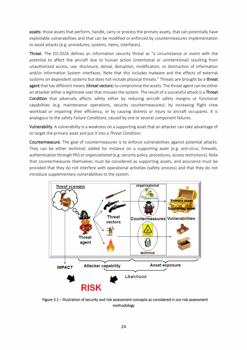
24
assets: those assets that perform, handle, carry or process the primary assets, that can potentially have
exploitable vulnerabilities and that can be modified or enforced by countermeasures implementation
to avoid attacks (e.g. procedures, systems, items, interfaces).
Threat. The ED-202A defines an information security threat as “a circumstance or event with the
potential to affect the aircraft due to human action (intentional or unintentional) resulting from
unauthorized access, use, disclosure, denial, disruption, modification, or destruction of information
and/or Information System interfaces. Note that this includes malware and the effects of external
systems on dependent systems but does not include physical threats.” Threats are brought by a threat
agent that has different means (threat vectors) to compromise the assets. The threat agent can be either
an attacker either a legitimate user that misuses the system. The result of a successful attack is a Threat
Condition that adversely affects safety either by reducing aircraft safety margins or functional
capabilities (e.g. maintenance operations, security countermeasures): by increasing flight crew
workload or impairing their efficiency, or by causing distress or injury to aircraft occupants. It is
analogous to the safety Failure Conditions, caused by one or several component failures.
Vulnerability. A vulnerability is a weakness on a supporting asset that an attacker can take advantage of
to target the primary asset and put it into a Threat Condition.
Countermeasure. The goal of countermeasures is to enforce vulnerabilities against potential attacks.
They can be either technical, added for instance on a supporting asset (e.g. anti-virus, firewalls,
authentication through PKI) or organizational (e.g. security policy, procedures, access restrictions). Note
that countermeasures themselves must be considered as supporting assets, and assurance must be
provided that they do not interfere with operational activities (safety process) and that they do not
introduce supplementary vulnerabilities to the system.
Figure 3.1 – Illustration of security and risk assessment concepts as considered in our risk assessment
methodology

25
Threat scenario. Establishing a threat scenario consists in identifying precisely what needs to be
protected (primary and supporting assets as well as existing countermeasures and their potential
vulnerabilities), against what (characterize the threat source profile) and why (to avoid or reduce the
impact of a Threat Condition).
Impact. The impact of a threat scenario is the consequence of a successful attack. In risk management,
the impact can be of diverse nature: business or economic losses, brand or personal image damaging,
sensitive information gathering and disclosure, privacy violation, etc. In the aeronautics, the only aspect
considered is security for safety. The impact is thus related to the feared events as they are considered
in aircraft safety, in terms of consequences on aircraft functional capabilities, crew workload and
passengers in case of failure condition (see table 3.1). Note that for each severity level a probability
quantity is provided to signify the maximum allowed value in the end of a safety Fault Tree Analysis
(FTA) graph and the associated Design Assurance Level (DAL) that stands for the accuracy dedicated to
the design and development of a system according to its criticality, it sets objectives to properly provide
assurance to certification authorities that developed system performs safely its intended functions. For
instance, a DAL A system will receive the maximum care as a failure would have a catastrophic impact,
whereas a DAL E system will have no design constraint as a failure would not have any consequence on
flight safety. Associated design and development rules are given by standards DO-178B for software and
DO-254 for hardware.
Severity
Failure Condition Effect
Probability DAL Functional capabilities
Crew workload Passengers
No effect No effect Frequent
=1 Level
E
Minor Slight
reduction Slight increase
Some inconvenience
Probable =10-3
Level D
Major Significant reduction
Significant increase, conditions impairing crew efficiency
Some discomfort
Remote =10-5
Level C
Hazardous Large
reduction
higher workload or physical distress such that the crew could
not be relied upon to perform tasks accurately or completely
Adverse effects
Extremely remote
=10-7
Level B
Catastrophic All failure conditions which prevent continued safe flight and
landing
Extremely improbable
=10-9
Level A
Table 3.1 – Failure Condition severity, probability objectives and assurance level according to SAE ARP-4761
Risk. There are many definitions and controversies about what a risk is and how to determine it either
qualitatively or quantitatively. In literature, risk is commonly defined as the product of three factors:
Risk = Threat × Vulnerability × Impact. In our case, we define the risk as the combination of the impact
of a successful attack and the likelihood of the occurrence of such an attack. The likelihood is itself
determined as the combination of the attacker capability and the exposure of the asset. The semi-
quantitative method to determine the risk level and the intermediate steps, is described in part 3.2.4.

26
Risk treatment. Based on ISO 27005:2011, the ED-202A draft proposes the following options to treat
completely or partly the security risk:
Avoid it: the system scope needs to be changed so that it will not be exposed any longer
Mitigate it: add technical requirements for security measures to be taken in order to reduce its
severity and/or its likelihood
Take it: endorse its consequences without further security countermeasures
Transfer it (or share it): transfer the responsibility to manage it to other organizations or share it
with other organizations
Risk avoidance or mitigation decisions are addressed by development teams, leading to revision of the
security scope and / or security protection.
3.1.2. STATE OF THE ART ON RISK ASSESSMENT METHODS
In this part, we aim at listing the particularities of some widespread risk assessment methodologies
based on ISO/IEC22 international norms (summarized in table 3.2) as well as research work on how to
characterize the risk, mentioned hereafter.
Contrary to organizational risk assessments that aim at consistent file production for countermeasures
justification and compliance to ISO security norms or legislation, research is rather focused on providing
representations, algorithms and tools in order to perform software-based automated risk analysis, with
quantitative risk estimations or threat probabilistic predictions. They take as inputs the three recurrent
factors “threats, assets and vulnerabilities” and combine them with more or less sophisticated models.
For instance in terms of representations, Liao et al. [49] propose a visual representation of threats under
a pyramidal form with three edges representing respectively the attacker’s prior knowledge about the
system (the most crucial parameter), the criticality of the area being attacked and the loss factor in
terms of privacy, integrity, business repudiation and financial loss to compensate damages whenever a
threat affects the system. Ortalo et al. [50] define a mathematical model based on Markovian chains to
define the METF (Mean Effort to security Failure). It is the security equivalent of MTTF (Mean Time To
Failure) that is the average time before a failure is detected in a system considering an infinite repair
time (contrary to the Mean Time Between Failures MTBF). The framework starts with attack state graphs
with a given transition rate 𝜆𝑘𝑖. Then the METF is computed as follows: 𝑀𝐸𝑇𝐹𝑘 = 𝐸𝑘 +
∑ 𝑃𝑘𝑖 ×𝑀𝐸𝑇𝐹𝑖𝑖∈𝑜𝑢𝑡(𝑘) , where 𝑃𝑘𝑖 = 𝜆𝑘𝑖 × 𝐸𝑘 and 𝐸𝑘 = 1/∑ 𝜆𝑘𝑖𝑖∈𝑜𝑢𝑡(𝑘) . Contrary to the failure rate
used in safety, determined by experience feedback and fatigue testing on components, security
parameters are not physically measurable, so the determination of some coefficients still remains
22 International Organization for Standardization / International Electrotechnical Commission
ISO/IEC 73: terminology, 13335: fundamental IT security concepts and models, 17799: guidelines for organizational IT risk
management, 15443: security assurance and effort to achieve confidence that IT security requirements and security policy are
satisfied; 2700X series: entirely dedicated to IT security management, 3100X series: principles, context and guidelines to
manage any kind of risk for any kind of organization no matter its size or its domain, 15408: also called Common Criteria [58],
most widespread reference in terms of IT security risk management that provides concepts, guidelines and criteria for the
evaluation of IT systems security properties.

27
subjective. Similarly, Alhabeeb et al. [51] provide a probabilistic method for real-time risk prediction
analysis based on fuzzy logic and Petri Nets. Roughly speaking, it consists on the one hand of IDS alerts
analysis and on the other hand, of the analysis of the vulnerability-scan sensors distributed in the
network. Once assessed, the IDS alerts and the vulnerabilities information are aggregated with different
weights, depending on pre-established trustworthiness rules, to compute the risk ratio and reducing
the amount false positives. Mahmoud et al. [52] developed an interesting quantitative algorithm based
on computation of risk propagation through each node of an airborne network. Some of the parameters
necessary for risk level determination are computed by using network vulnerability scanning. The total
risk of a network is computed by summing the risk incurred by each node. The 𝑖𝑡ℎ node risk is expressed
by: 𝑅𝑖 = 𝑉𝑖 × (𝑅𝑖− + 𝑅𝑖
+). 𝑅𝑖− is the individual risk of node 𝑖, based on the sum for each vulnerability of
node 𝑖 of the product threat likelihood × impact. And 𝑅𝑖+ is the propagated risk, i.e. the sum for all
nodes around 𝑖 presenting vulnerabilities of the propagation likelihood and propagated impact. Finally,
𝑉𝑖 is the Value of node 𝑖 and is computed by multiplying the number of nodes around 𝑖 by the cost
(valued between 0 and 9) and the severity linked to the aircraft domain (ATS, AOC, AAC, APC) of node 𝑖.
Note that node cost and severity are the only values requiring “a human in the loop” as impact values
are taken from the CVSS severity of CVE23 public database and elements for propagation are taken from
the network statistics tool Netstat.
Discussion. On the one hand, the methodologies presented in table 3.2 could fit to the needs whenever
the scales and stakes are adapted to the aeronautic context. If the aeronautic industry requires to have
its own methods it is mainly for financial reasons. Indeed common security evaluation methods require
either to be lead by certified analysts (for instance ISO 27005 certification, EAL evaluation of products)
or specific tools that are rather expensive.
On the other hand, the presented research methods are useful for an a posteriori evaluation because
the system must have been implemented or at least emulated to be able use them. They are not
adapted to an early design process, which was one of the main requirements for the methodology
presented in this chapter. Also, they are based on known vulnerabilities databases (e.g. CVE) and do not
consider novel/emerging ones specific to aircraft airborne systems. Concerning the methodologies
described in table 3.1, we notice that they have several drawbacks: their complexity: all of them allow
handling risks at all possible levels, from risk assessment on information systems to risk management
within an entire organization, whereas the analysis we aim at doing is more focused on the technical
risk assessment of aircraft architectures, and eventually on giving some advices for organizational
procedures to deploy in the aircraft context of use. That is the reason that made us working on a very
simple, clear and guided methodology. It has to be mentioned that it very expensive and time consuming
to lead a risk assessment due to the volume of documentation to be produced, all the required
meetings, questionnaires and the amount of actors that are involved.
23 Common Vulnerabilities and Exposures: http://cve.mitre.org/

28
ASSESSMENT ELEMENTS
METHODOLOGIES Asset Threats Vulnerabilities Impact Occurrence Risk Tools
MAGERIT [53]
Provides a detailed list of processes, activities
and tasks for semiquantitative evaluation and
management of risk on Information Systems
Security dimensions:
availability
integrity
confidentiality
authenticity
accountability Asset value:
negligible=0
low=2
medium=5
high=8
very high=10
Degradation of asset value: 1%, 50%, 100 %
Provides a mapping between misuse incidents and attacks as well as a list of threats applicable per asset
N/A
Evaluated by a table combining
asset value vs.
degradation level
Frequency:
100-VH-daily
10-H-monthly
1-M-annually
1/10-L-every few years
determined by the
combination of
impact vs.
frequency
XML modeling, use of tables, attack trees,
cost/benefit analysis, data flow, process charts and other
graphical techniques. No guidelines for requirements.
CRAMM [54]
(CCTA24 Risk Analysis and Management
Method) deals with risk assessment on
Information Systems within large organizations
Valued depending on the impacts of their
availability, integrity or confidentiality loss,
destruction or modification
Helps to continuous security management and improvement by
targeting specific threats to be put under
surveillance.
N/A
Economic losses evaluation
and/or
questionnaires
aimed at users
N/A
Recommends quantitative evaluation but
provides a scale from
“very low” to “high”
Associated with a software tool that
proposes a list of 3000 counter-measures
depending on risk type, severity and security level to be achieved.
NIST 800-30 [55]
800-series Special Publications of the
National Institute of Standards and
Technology (USA) within large organizations that
process Federal sensitive information in their IT
facilities
No asset identification, the only
assets are “Federal sensitive information”
Sequence of tactics, techniques &
procedures (TTPs) employed by
adversaries and likelihood of success
Characteristics
(capability, intent) and likelihood of initiation
Severity in the context of predisposing conditions (at information,
architectural, functional, operational and
environmental levels) that increase or
decrease likelihood with pervasiveness
Magnitude
Uncertainty: (i) how future will resemble the past (ii) incomplete knowledge of threat (iii) undiscovered vulnerabilities (iv) unrecognized dependencies
impact vs.
likelihood of occurrence
(as a combination
of the likelihood of initiation and likelihood of
success)
All elements evaluated with the qualitative &
semi-quantitative values: Very High (96-100 or 10), High (80-
95 or 8), Moderate (21-79 or 5), Low
(5-20 or 2), Very Low (0-4 or 0).
24 Central Computer and Telecommunications Agency

29
OCTAVE [56]
(Operationally Critical Threat, Asset and
Vulnerability EvaluationTM)
The assets are the information exchanged
within the company.
N/A
It proposes two security approaches:
#1: a reactive one
consisting in vulnerability management
(identification and patching)
Aims at avoiding financial losses
and brand reputation
damage
#2: a proactive one consisting in risk identification and management.
N/A
The methodology provides guidance for
leading assessment workshops that require the participation of all
actors to build a consistent decision and
justification file.
MEHARI [57]
(Method for Harmonized Analysis of
Risk) Set of checklists &
questionnaires to assess risk at 8 levels of an organization: entity
(services), site, buildings, applications & processes, systems & infrastructure, development life-cycle,
software products, networks &
communications.
Assets:
primary (processes, information)
supporting (premises, offices, IT & networks)
Stakes & assets classified according to
the availability, integrity, confidentiality
criteria
Natural exposure levels of assets
N/A
Impact on business of vulnerabilities exploitation
4 impact levels:
none,
impact of deteriorations,
impact of dysfunctions,
impact of final losses centered on business
N/A impact
vs. potentiality
Downloadable* Excel worksheets with a set of
checklists and evaluation grids. Note
that the audit questionnaire contains
14 worksheets of 100 to 200 questions each!
*http://www.clusif.asso.fr/en/production/meh
ari/download.asp
EBIOS [58]
Simple risk evaluation (IT products & organization
management) through the qualitative
characterization of security criteria, security
needs, likelihood and impact severity
Primary assets’ security needs
expressed in terms of availability, integrity and
confidentiality
It provides a knowledge base with a wide spectrum of generic threats and vulnerabilities, and
countermeasures covering from industrial espionage to natural disasters.
Threat sources are characterized by considering the attacker’s motivations
Impact on missions, persons, financial, juridical,
image, environment, etc.
Assessment of the likelihood
(threat opportunity) with qualitative scales to be set by the
evaluator
Impact vs.
Likelihood
Gives advices on how to build an action plan involving all the actors
of the organization. Each organization is meant to self-build its own scales depending on the stakes
of the analysis.
Table 3.2 – Summary of different risk management methodologies assessment elements

30
3.2. RISK ASSESSMENT FRAMEWORK DESCRIPTION
Ideally, a security assessment should guarantee that all potential scenarios have been exhaustively
considered. They are useful to express needed protection means and to set security tests for final
products. This part describes our six-steps risk assessment methodology summarized in Figure 3.3. This
methodology is inspired in some elements of the ones presented in §3.1.3 and mainly EBIOS regarding
the use of qualitative scales for likelihood and the notion of threat opportunity that we tuned into two
notions: the attacker capability and the asset exposure, these scales being exclusively adapted to the
aeronautics domain and compliant with the ED-202 and ED-203. If we summarize it briefly, this
methodology consists in modeling the context of the analysis in order to identify threat scenarios using
a dual method (top-down and bottom-up) inspired on safety tools. Then, these threat scenarios are
evaluated with an adaptable qualitative and quantitative risk estimation method to determine their
likelihood, their potential impact and whether the risk is acceptable or not. Whenever the risk is not
acceptable, the requirements for countermeasures must be formalized and associated to a Security
Level (SL) to indicate the effort to counter such threat. Finally, the countermeasure must be
implemented and the whole system must be evaluated again, considering the added countermeasure.
The detailed description of each step is given hereafter.
PerimeterSecurity Policy Use cases
Threat conditions
Likelihood Safety Impact
Acceptability?
Security Level Security objectives
Assurance
Requirements
Security Functional
Requirements
Countermeasures
SL
assig
ned
Threat scenarios
Secured
architecture pattern
Integration
in system’s
architecture
NO
Attacker capability Asset exposure
Security rules
Best
location
Security basis Development processSecurity process
Data and functions
(primary assets)
Soft/Hardware
items, components
(supporting assets)
Known attacks and
vulnerabilities
Context
Establishment
Preliminary Risk
Assessment
Vulnerability
Assessment
Risk Estimation
Security
Requirements
Risk Treatment
1
2
3
4
5
6
Top-down approach
Bottom-up approach
Exposure
criteria to
be reduced
Traceability
Figure 3.3 – Risk assessment and treatment process: the figure differentiates input data for the security process
as coming either from the development process or from a security knowledge basis.

31
3.2.1. STEP 1: CONTEXT ESTABLISHMENT
Preliminary to any analysis, a precise overview of the security perimeter is required to focus the analysis,
avoid over-design and define roles and responsibilities. For a better understanding of the perimeter
information, we prone a graphical representation (e.g. in UML) to gather and highlight functional
interfaces and interactions. Some of the input elements of a risk analysis shall be:
security point of view: whether we address security for safety, airline branding protection, or
passenger privacy (credit card transactions protection), etc., it has to be clearly expressed, because
it will imply the use of other IT security standards than only the airworthiness security ones.
depth of the analysis: whether if the analysis is made at aircraft level, system or item level.
functional perimeter: knowing the functional perimeter of the analysis allows identifying the
primary assets, i.e. the critical data and functions which loss could have hazardous consequences.
system architecture: if it is available, the architecture will allow identifying the supporting assets,
i.e. those that deal with critical data (i.e. primary assets) and contribute in performing critical
functions as well as the different interfaces between them.
operational use cases: the operational use of the systems and/or items must be detailed, not only
during flight phases but also during maintenance operations on ground.
interfaces and interactions: allows identifying the potential sources where an attack could be
originated and its potential propagation throughout the human-system and system-system
interfaces.
assumptions: concerning the environment and users, usually, pilots are considered as trusted, but
it is up to the analyst to define whether the airport environment and its different users are trusted
or not and make the analysis accordingly.
initial security countermeasures: if applicable, initial countermeasures must be identified and
considered as assets.
external dependencies and agreements: if the analysis is made at system level, it is necessary to
identify teams responsible for lower-level (i.e. item level) and higher-level (i.e. system of systems
or avionics suite level) risk assessment and the associated documents to ensure proper traceability
and eventual risk transfer.
Once all important input data has been collected in step 1, threat scenarios can be established. To
improve exhaustiveness and accuracy, we prone the use of two approaches: on the one hand, a top-
down approach where parting from Threat Conditions on primary assets, misuse or intended attacks on
supporting assets are deduced downgrading from aircraft level to systems, subsystems and items. On
the other hand, a bottom-up approach allows from potential vulnerabilities on items to follow the
consequences of their exploitation up to the aircraft level.
3.2.2. STEP 2: PRELIMINARY RISK ASSESSMENT (TOP-DOWN APPROACH)
Preliminary Risk Assessment is an early design activity which goal is to assess designers so they consider
main security issues during the first steps of avionic suite architecture definition. Basically, it aims at
identifying what has to be protected (primary assets) against what (threat conditions). At this step,
system architecture can be still undefined, as it is a high-level functional analysis.

32
Primary assets identification. First of all, primary assets are identified from the Functional Hazard
Assessment (FHA). The FHA is an early development and high-level25 safety analysis based on ARP-4761
that consists in classifying the Failure Conditions applicable to aircraft functions depending on their
severity. Systematically, the functions appearing as critical are the primary assets.
Threat Conditions identification. If some of the Failure Conditions considered in the FHA can be
originated intentionally, they are also considered as Threat Conditions. Failure Conditions are expressed
in terms of integrity or availability loss (e.g. function, erroneous, loss, delay, failure, mode change,
unintended function, inability to reconfigure or disengage, wrong information, right information at the
wrong place, etc.). In the same way, we propose a generic list of Threat Conditions (table 3.4), their
severity is evaluated with the same criteria as Failure Conditions (cf. table 3.1).
Threat Condition Class Definition
Failure Conditions
Wrong function Intended function is performed incorrectly or not provided when or where needed (e.g. false alarm).
Loss of function Intended function is not performed or intended information is not provided, in security, it can be caused by a Denial of Service attack.
Misuse Erroneous input data or unintended function being invoked by an authorized entity.
Confidentiality loss (or Compromise)
In case of information exposure, data can be intercepted. Having access to certain information could give clues on system breaches and on how to lead an attack. An attacker can use existing sniffing and footprint tools such as network scanners to perform reconnaissance and get sensitive information.
Bypass
Gain of unauthorized access even through security countermeasures. Common attacks can be active (e.g. cracking a password by brute force) or passive (e.g. rights usurpation through trap/backdoors). Also known as impersonation, masquerading, or escalate privilege.
Tamper Intended function appears to be performed correctly but is incorrect, or information is incorrect but satisfies safety integrity mechanisms. Includes coherent corruption and repudiation (i.e. hiding clues of an attack).
Spoofing Intended information appears to be correct and correctly sent, but either source or destination is incorrect (e.g. traffic redirection).
Subversion Loading of unsigned software or malware into the system (code needs to be signed, software sources must be traceable, software development practices as well and data-loading procedures must be followed).
Malware Presence of malware in the system (coming either from development or introduced by loading).
Open security failure Security countermeasure allows unauthorized access (bypassing).
Closed security failure Security countermeasure disallows authorized access.
Table 3.4 – Threat Condition Classes (proposal)
Top-down approach for Threat Scenarios Definition. Similarly to the safety deductive Fault Tree Analysis
(FTA), the security Preliminary Risk Assessment follows a top-down approach: parting from a feared
event (i.e. a Threat Condition) on a primary asset, all the potential attack or misuse causes leading to it
are considered, deducing them at system-of-systems level (e.g. aircraft or avionic suite), down to
systems and sub-systems. Due to the similarities with Functional Hazard Assessment (FHA) made in
safety process and as a matter of time and cost saving, this assessment can be common both to safety
and security preliminary processes. In practice, a mapping of the dependencies between critical
25 Only performed at system and eventually sub-system level

33
functions and the associated data must be performed. This will help to find the path followed by the
critical data, i.e. from its origin (e.g. sensor where the data is collected, software download tool, HMI,
air-ground communication systems) to the system that will use it to perform the critical function. The
goal is to identify the supporting assets at system and subsystem levels as the primary asset could be
accessed by exploiting a supporting asset vulnerability.
3.2.3. STEP 3: VULNERABILITY ASSESSMENT (BOTTOM-UP APPROACH)
Once the architecture has been defined and the implementation choices are known, all supporting
assets associated to a given primary asset are identified in this third step. It has to be verified if the
supporting assets are protected by countermeasures and if they contain known vulnerabilities. We
prone the use of a generic checklist of vulnerabilities. For instance, the public database CVE26 (Common
Vulnerabilities and Exposures) lists the vulnerabilities applicable in widespread IT products (laptops,
smartphones, anti-viruses, servers, web interfaces, protocols, etc.). While the latter is useful to identify
vulnerabilities on COTS, it is necessary to lead intrusion testing on dedicated aeronautical equipment to
complete this checklist.
Bottom-up approach for Threat Scenarios Definition. Similarly to the safety inductive approach of Failure
Mode and Effect Analysis (FMEA), where every possible failure at item level is considered to guess its
consequences at sub-system, system and system-of-systems level. In the security vulnerability
assessment, the bottom-up approach aims at identifying potential security vulnerabilities in supporting
assets at item level, particularly targeting human-machine and system-system interfaces. First with
vulnerability checklists identification and then by intrusion testing, threat propagation paths must be
followed to determine the consequences of each item vulnerabilities exploitation on sub-systems,
systems and systems-of-systems level.
To summarize, the top-down approach allows the identification of high-level security requirements and
their progressive declination into more detailed ones, whereas the bottom-up one, allows validating
and completing these requirements with both technical constraints and effectiveness requirements, as
well as identifying threats and vulnerabilities left unconsidered during the top-down analysis.
3.2.4. STEP 4: RISK ESTIMATION
As it is impossible to handle all identified threat scenarios, it is necessary to rank them by criticality. We
define the risk of a threat scenario as the combination of its likelihood and its safety impact, and
likelihood itself as the combination of two factors: the attacker capability and the asset exposure. These
are semi-quantitative factors that we introduced to evaluate the likelihood level, i.e. the potential
frequency of a threat scenario.
Let 𝑋 = {𝑋1, … , 𝑋𝑛} be a set of 𝑛 qualitative attributes chosen to characterize the attacker capability
and similarly 𝑌 = {𝑌1, … , 𝑌𝑧} a set of 𝑧 qualitative attributes chosen to characterize the asset exposure.
Each attribute 𝑋𝑖 can take 𝑚 values: {𝑋𝑖1, … , 𝑋𝑖
𝑚}, 𝑋𝑖𝑗 being more critical than 𝑋𝑖
𝑗−1. To each qualitative
value 𝑋𝑖𝑗, we associate quantitative severity degrees 𝑥𝑖
𝑗, with 𝑥𝑖
𝑗>𝑥𝑖𝑗−1
.
26 http://cve.mitre.org/

34
For instance:
𝑋 = {𝑋1 = “elapsed time to lead the attack”, 𝑋2= “attacker expertise”, 𝑋3= “previous knowledge of the attacked system”, 𝑋4= “equipment used”, 𝑋5= “attacker location”}.
𝑋1 can take the values: {=">day", 𝑥1
1=0 ="<day", 𝑥1
2=1
="hours", 𝑥13=2
="minutes"} 𝑥14=3
Let us call 𝑓𝑗() the evaluation function performed by the security analyst to assign the corresponding
severity degree 𝑎𝑖 to each 𝑋𝑖 for a given threat scenario: 𝑎𝑖 = 𝑓𝑗=1𝑚 (𝑥𝑖
𝑗). The attacker capability score is
expressed for each threat scenario by the normalized sum of the values assigned to all attributes of set
𝑋 (see equation 1).
A =∑ (𝑎𝑖)ni=1
∑ (𝑥𝑖𝑚)n
i=1
, 𝑥𝑖𝑚 ≥ 𝑥𝑖
𝑗, ∀𝑖 = 1…𝑛, ∀𝑗 = 1…𝑚
(1)
Exactly the same reasoning is made to express the asset exposure.
Attacker capability attributes. The attacker capability stands for the strength to lead an attack. It can be
defined by its expertise, the threat vectors used, his knowledge of the system, the motivation of the
attack, etc. Note that the attributes listed in table 3.5 are just examples and thus not exhaustive.
Depending on the analysis context more attributes and more values can be added. Indeed, whether we
want to protect the In-Flight Entertainment system against script kiddies or the core avionics critical
systems against cyber-terrorist, the evaluation criteria will not be the same.
Values
Attributes 3 2 1 0
X1: Elapsed time for the attack minutes hours <day >day
X2: Attacker expertise employee layman proficient expert
X3: Attacker system knowledge public restricted sensitive critical
X4: Equipment used none domestic specialized dedicated
X5: Attacker location off-airport airport cabin cockpit
Table 3.5 – Attacker capability attributes (example)
To determine the severity values, we have reasoned in terms of frequency: the more an attack is likely
to occur often and the more the attacker capability score value will be high. For instance, it is more likely
to have frequent attack attempts from script kiddies (i.e. people who don’t have real skills in security
but that try to infiltrate systems just for fun) than from criminal/terrorist organizations. Table 3.5 just
provides an example of set of attributes; the goal is that the security analysts define their own attributes
and scales.
Asset exposure attributes. Following the same principle, we can build a table (e.g. table 3.6) to measure
to what extent an asset is exposed (i.e. accessible) to attacks. This is the crucial point where the
aeronautical and environmental context must be clearly expressed. For this table we have not reasoned
in terms of frequency but in terms of restriction: the more the access to the asset is restricted (physically
and in terms of system and vulnerabilities knowledge) and the more the severity values and thus the
asset exposure score will be low.

35
Values
Attributes 4 3 2 1 0
Y1: Asset location off-aircraft cabin maint. facility cockpit avionic bay
Y2: Class27 of asset class 1 class 2 class 3
Y3: DAL DAL E DAL D DAL C DAL B DAL A
Y4: Vulnerabilities large public limited public not public unknown none at all
Y5: Countermeasure none organizational technical on asset >2 on chain
Table 3.6 – Asset exposure attributes (example)
Likelihood. It is the qualitative estimation of the potential frequency of occurrence of a threat scenario.
First, the ED-202 considered five likelihood levels: 'pV: frequent', 'pIV: probable', 'pIII: remote', 'pII:
extremely remote', 'pI: extremely improbable' but does not provide guidelines on how to determine
and justify them correctly. As they are too subjective to be directly determined, we built table 3.7 to
assign a likelihood level to the combination of attacker capability (A) and asset exposure to threats (E)
semi-quantitative values. Note that table 3.7 is usable whatever the amount of attributes required, and
whatever the number of values each attribute can take, i.e. this framework allows flexible evaluation
criteria as they may vary according to the context (aircraft or system level, special environment
conditions, threats evolution). However, these criteria must be defined with an accurate taxonomy so
the evaluation is exhaustive, unambiguous and repeatable.
Attacker capability score
0 ≤ A ≤ 0,2 0,2 < A ≤ 0,4 0,4 < A ≤ 0,6 0,6 < A ≤ 0,8 0,8 < A ≤ 1
Exp
osu
re 0 ≤ E ≤ 0,2 pI pI pII pIII pIV
0,2 < E ≤ 0,4 pI pI pII pIII pIV
0,4 < E ≤ 0,6 pII pII pIII pIV pV
0,6 < E ≤ 0,8 pIII pIII pIV pV pV
0,8 < E ≤ 1 pIV pIV pV pV pV
Table 3.7 – Attack likelihood through attacker characteristics and asset exposure (proposal)
Acceptability. To determine whether a risk is acceptable or not, and measure the effort to be provided
to avoid the most likely and dangerous threats, we propose the acceptability risk matrix (table 3.8) that
associates safety impact and likelihood. Safety impact levels are the ones defined in table 3.1: 'N/E: no
safety effect', 'MIN: minor', 'MAJ: major', 'HAZ: hazardous', 'CAT: catastrophic'.
Safety Impact
No Effect Minor Major Hazardous Catastrophic
Like
liho
od
pV: Frequent Acceptable Unacceptable Unacceptable Unacceptable Unacceptable
pIV: Probable Acceptable Acceptable Unacceptable Unacceptable Unacceptable
pIII: Remote Acceptable Acceptable Acceptable Unacceptable Unacceptable
pII: Extremely Remote Acceptable Acceptable Acceptable Acceptable Unacceptable
pI: Extremely Improbable Acceptable Acceptable Acceptable Acceptable Acceptable* * = assurance must be provided that no single vulnerability, if attacked successfully, would result in a catastrophic condition
Table 3.8 – Acceptability risk matrix (proposal)
27 class 1: Portable Electronic Device (PED); class 2: modified PED; class 3: installed equipment under design control.

36
3.2.5. STEP 5: SECURITY REQUIREMENTS
Once threat scenarios have been established and the risk acceptability evaluated, the security level as
well as the countermeasures effectiveness and assurance requirements must be assigned.
Security Level (SL). The SL is similar to safety Design Assurance Level (DAL) defined in DO-178B. It is
applicable both to the countermeasure to be implemented and its requirements. SL has a dual
signification, it stands both for:
strength of mechanism (assurance must be provided that countermeasures perform properly and
safely their intended security functions)
implementation assurance (assurance must be provided that security countermeasure has followed
rigorous design and implementation process)
For each non acceptable threat scenario identified, a SL is determined based on the risk reduction
required so that risk becomes acceptable in table 3.8. Depending if the likelihood has to be reduced of
0, 1, 2, 3 or 4 levels to be on an acceptable level, SL will respectively take the values E, D, C, B or A. The
SL is assigned to each developed countermeasure and associated assurance requirements are meant to
be provided by the ED-203, once it will be released.
Security Requirements. For each unacceptable threat scenario, a set of security objectives to be fulfilled
are established. As there are still no specific rules to write security requirements for airborne systems,
these security objectives can be translated into security requirements using the Security Functional
Requirements (SFR) classes of Common Criteria [59] part 2 in order to have an initial template to express
security requirements in a formal way. Indeed, Common Criteria provide a classification of requirements
patterns and the inter-dependencies between them are already traced.
Assurance Requirements. Proving that security requirements have been respected is not enough;
development assurance must be consistent with a given environment and procedures quality. To do so,
each SL can be mapped with Common Criteria EALs (Evaluation Assurance Levels) as shown in table 3.9.
Each EAL is linked to a set of assurance families themselves composed of SARs (Security Assurance
Requirements). Assurance requirements aim at establishing accurate development rules so that security
functions perform correctly their intended purpose and means to maintain security during
development, maintenance and operational use have been taken into account. A list of assurance
requirements corresponding to each SL should be provided in the ED-203.
3.2.6. STEP 6: RISK TREATMENT
Countermeasure selection. Countermeasures must be selected for their compliance towards security
requirements and for their effectiveness, but also taking into account development costs in order to
avoid over design. Once a countermeasure has been developed on the most exposed supporting asset,
verification such as intrusion tests must be performed on the basis of threat scenarios to prove its
conformity with security requirements. Both countermeasures and intrusion tests should be made
according to the assurance requirements that will be provided by the ED-203, otherwise, Common
Criteria’s vulnerability assessment is suitable.

37
Security Rules. Safety process counts on a set of “safety rules” to provide for integrity or availability loss
ensuring a fail-safe state of the systems. For instance, continuous monitoring, reconfiguration,
redundancy (duplex, triplex, etc.), voting or comparison and dissimilarity are some of these rules. The
Common Mode Analysis (CMA) is then performed to verify the correct and safe construction of the
architecture. The same way, in order to ease security architecture design, “security rules” can be set
around principles such as: passive (e.g. monitoring) or active defense, perimetric defense (e.g.
authentication means at Human-Machine Interface level or at any equipment receiving external data or
software), middleware defense (e.g. filters at switch or router level), “onion skin” defense (e.g. at each
system interface of a functional chain or potential attack path), central defense (e.g. centralized decision
system), etc. Formal verification methods such as CMA could be then deployed to verify security rules
for architecture patterns construction have been correctly applied (e.g. respect of segregation between
critical and non-critical data in a router). These rules and verification means are still left to be defined.
3.3. SECURITY PROCESS
Defining a risk assessment methodology was urgent to answer the CRIs security objectives, but another
task we were assigned was to extract from the standards under construction (ED-202 and ED-203) the
activities and output documents for the future security process. We collaborated in the SEISES28 project
to insert these security activities into the actual development process. The basic idea has been to
identify the development activities defined in the DO-178B and DO-254 standards, the safety activities
from the ARP-4754 and finally the security activities from the ED-202 and ED-203 drafts at different
granularity levels (System of Systems, System and Item) and then link the activities of the three
processes together. This work resulted in the constitution of the triple V-cycle shown in figure 3.4, that
also includes the risk assessment activities.
28 Systèmes Embarqués Informatisés, Sûrs et Sécurisés (translation: computerized safe and secure embedded systems) is an
Aerospace Valley collaborative project between Airbus, Rockwell Collins, Astrium, Serma Technologies, Apsys, EADS, Onera, DGA, Thales Avionics, LSTI, LAAS-CNRS for the definition and linking of safety and security processes’ activities for embedded systems.

38
Figure 3.4 – Triple V-cycle with the activities of the safety (green), development (blue), security (red) processes
and their interactions.
Note that this contribution has not a real methodological or scientific interest, but is mentioned here as
an important industrial contribution for the company. To view the details of the triple V-cycle please
refer to appendix 2.
3.4. CHAPTER SUMMARY
In this chapter we have described our industrial contribution and its insertion in the overall development
process. The challenges of such a methodology were that it had to be easily interfaced with aeronautics
standards and practices (development cycle and safety process activities), and also not overwhelmingly
constraining but still providing easy guidelines for a domain that just starts getting introduced to cyber-
security issues.
The risk assessment methodology output is to provide security requirements for the airborne systems
protection that combined with the security objectives of Certification Review Items or Special
Conditions leads us to the common need for intrusion observation in order to: detect and characterize
anomalies taking place in the network to get a better knowledge of the potential threat that could occur
on board and eventually provide information for a real-time response to detected anomalies and to
verify the efficiency of implemented countermeasures or enforcing security functions such as firewalls,
as well as ensuring the airworthiness continuity.
System of Systems (SoS) level activities
System level activities
Item level activities

39
4. 4.
CHAPTER 4
THEORY ON SECURITY AUDIT
This chapter aims at providing an overview on the principles and algorithms used for anomaly or
intrusion detection systems (ADS/IDS). After defining what an IDS is, we describe the two main Machine
Learning classification techniques based on supervised and on unsupervised learning, as well as the one-
class classification methods. Then, we discuss about the importance and criticality of selecting the
adequate features to model the normal traffic behavior, and the treatment of the data to obtain an
optimum result. Finally, we provide an insight of Support Vector Machines’ theory and on the One Class
SVM algorithm that we are using in our own framework for intrusion detection.
4.1. STATE OF THE ART ON INTRUSION DETECTION SYSTEMS
4.1.1. MISUSE VS. ANOMALY DETECTION, BEHAVIORAL ANALYSIS JUSTIFICATION
Intrusion Detection Systems (IDS) can be classified as Host IDS (HIDS) or Network IDS (NIDS). HIDS check
system files’ integrity, user privileges, input/output traffic and log files from computer processes or
system audit agents to detect any abnormal behavior on the use of a device (e.g. anti-viruses). NIDS
scan the network looking for malicious packets or flows that violate for instance protocols policies (e.g.
snort [60] for packet-based inspection, BRO [61] for flow29 analysis or IDIOT [62] that uses Colored Petri
Net for pattern-matching). There are also hybrid approaches that combine HIDS and NIDS such as
Distributed IDS (DIDS) [63]. Most of the commercial IDS previously mentioned are signature-based
techniques, i.e. they require a database of prior encountered attacks or a set of pre-established rules to
perform pattern-matching and prevent security policy violation (e.g. malware signatures in anti-viruses
or filtering rules in firewalls looking for string signatures in payloads, frequently-attacked ports or
specific header signatures). Such IDS have the advantages of being very accurate, they generate few
false alarms, and the nature of the attack is well described within its environment, which eases eventual
preventive or corrective actions. But, these countermeasures have seen their performances decrease
with the new attacks sophistication, elaborated enough to bypass conventional security
countermeasures (e.g. polymorphic viruses). The drawbacks of signature-based techniques are that
they require frequent update of their attack database as they basically rely heavily on them, such
signatures are time-consuming and expensive to obtain as they are extracted “manually” by a security
29 A flow being determined by the 5-tuple: IP source & destination addresses, port source & destination and protocol.

40
expert inspection, also, the difficulty of defining generic attack signatures makes that, very often, they
are effective in a very precise environment. What is more, such IDS cannot detect 0-days (i.e. novel)
attacks and they generally deal with incoming attacks rather than outgoing or global network threats.
That is the reason why anomaly-based IDS (ADS) were introduced to perform statistical measures among
network traffic to obtain behavioral model accurate enough to detect anomalies by often using Data
Mining techniques. Anomaly-based IDS consist in observing a deviation from a previously learnt normal
or expected behavior of the system. Network Behavior30 Analysis (NBA) solutions have been developed
to detect anomalous behaviors in networks. They aggregate data from different nodes of the network
(usually hubs, routers, switches) for offline analysis, for instance under Netflow [64] format. The threats
that can be detected with such techniques are mainly protocol anomalies, probes, Denial of Service
(DoS) and Distributed DoS attacks. ADS clearly present the advantage of being able to discover novel
attacks and of being generic because they do not require updates of hard-coded signatures, although
the normal traffic behavior model might require updates, this can be done in a more autonomous way.
However, the fact of considering every occurrence that does not correspond to a previously learnt
normal behavior as an anomaly induces a high risk of false alarms; also, behavior can gradually evolve
in time and thus increase the amount of missed anomalies. A survey on IDS commercial techniques
made in 2009 [65], showed that out of the 25 compared IDS, 100% of them were signature-based and
only 7/25 introduced anomaly-based concepts. It has to be noticed that anomaly-based IDS’s goal is not
to replace signature-based IDS but just to complete them. However, ADS are said to still lack of accuracy,
as a matter of fact Owezarski [66] proved that some of them are slightly better than a random detection
process (i.e. tossing a coin to determine whether an instance is malicious or normal). In this chapter, we
focus on ADS and more particularly on those using Machine Learning techniques to detect normal or
anomalous patterns in network traffic.
What is Machine Learning? Machine Learning is an Artificial Intelligence field in which computers are
meant to deduce rules from patterns found in traffic observation and processing. It aims at improving
program’s own understanding of the data without providing readable output, whereas the fact of
extracting rules and information for human comprehension is rather called data mining. Data Mining
consists in the analysis of a huge quantity of data in order to extract a model and knowledge (statistics)
from it. Each step arises many questions: raw data generation (data types, sample size, online/offline),
preprocessing (normalization, scaling, missing values, feature selection/extraction), Machine Learning
(hypothesis and choice of learning paradigm/algorithm), hypothesis validation (cross-validation, model
deployment), etc. Alex Smola, in its Introduction to Machine Learning [67], says that the “art of Machine
Learning is to reduce a range of fairly disparate problems to a set of fairly narrow prototypes [...] science
of Machine Learning is then to solve those problems and provide good guarantees for the solutions.”
Machine Learning problems can be of four different kinds: association (find relationships or
dependencies between instances), regression (for numeric prediction), classification (assign a given
class to samples depending on their characteristics) or clustering (grouping similar instances together).
In the context of this PhD, the solutions we focused on are classification and clustering algorithms
respectively used for supervised and unsupervised learning. These techniques are more closely
described in the rest of the chapter, but before, let us have a look to what is the state of the art in terms
of airborne networks audit.
30 Behavioral modeling is used for many applications such as: fraud detection, fight against terrorism, epidemiology analysis
or even to target potential consumers on social networks by providing adapted advertisements.

41
4.1.2. RELATED WORK CONCERNING SECURITY MONITORING IN AIRBORNE NETWORKS
If we take a look among the actual research on airborne security, there are very few articles dealing with
security anomalies or threat detection systems. Among them, the oldest document we found [68] dates
back to 1989, it sets specifications for an embedded avionics audit function in order to detect and deter
penetration of security controls by unauthorized subjects, i.e. a HIDS based on attributes such as the
number of failed password attempts. The audit function is performed by a Trusted Kernel or Trusted
Computing Base (TCB) that reviews patterns of objects accessed by subjects and detects security
measures bypassing, escalate privileges by unauthorized users, preventing unauthorized operations. A
very important notion is also that the TCB records all actions to avoid non-repudiation. However, this
“old” document does not give more details on the context of threats that lead the authors to work on
that subject. Maybe because the majority of the paper is dedicated to the compression algorithm for all
security violations data storage which was a very challenging issue at that time. Ali et al. [69] proposed
in 2004 an anomaly-based IDS as a complement to the existing signature-based IDS for an airborne
threat detection. It uses snort with a pre-processor plug-in that assigns an anomaly score based on
observed history of the network. For instance, the fewer times an occurrence has been observed in the
past, the higher the anomaly score is, or depending on the source/destination IP addresses and ports, a
different anomaly score is assigned. The system maintains a table with the occurrences of different
events and their related probability with higher weight for recent events. It has different detectors that
look for individual packets targeting for instance closed ports, dead destination IP addresses or unusual
combinations which seems to be rather similar to a filter. But we found no airborne security audit
function that used Machine Learning. We imagined that it could come from the controversy of certifying
a system using what we could qualify as an Artificial Intelligence (AI) technique in an aircraft which is
exclusively composed by deterministic systems. However, it has to be noticed that such techniques are
actually under research to be introduced on aircrafts for other applications such as: aircraft fuel
consumption prediction [70], weather diagnosis to avoid turbulences [71], aircraft health monitoring
[72] such as commercial aircraft operation performances monitoring in terms of engines information,
sensors signals, etc. [73] to perform aircraft safety diagnosis and generate alerts so that the ground
crew is aware of any abnormal situation, intelligent processing of sensors data in unmanned
autonomous systems in the airspace [74].
4.1.3. MACHINE LEARNING ALGORITHMS AND RELATED ANOMALY DETECTION TECHNIQUES
The basic assumptions made in cyber-security anomaly detection are that, on the one hand, attacks
forcefully differ from normal traffic behavior, because attacks exploit vulnerabilities that are hidden and
thus seldom used in normal behavior. On the other hand, malicious occurrences are rare, i.e. they are
a very small proportion of the “normal” traffic. Looking for such few and different events is known as
outlier detection problem. Outlier detection is either distribution-based or distance-based. In the
context of this PhD, we desire to build a model from the relationships between the variables used to
describe the network traffic in its normal configuration in order to make classification prediction of new
traffic samples and be able to determine whether it is normal or anomalous. Although most of the
algorithms presented hereafter are both used for regression (when the output is a number) and for
classification (when the output is a class label) problems, we will only focus on their classification
principles and capabilities. In Machine Learning there are three main classification techniques to learn
and model a behavior: supervised, unsupervised and semi-supervised learning techniques. Supervised

42
techniques require a training phase with a labeled training data set, i.e. a data set where the nature or
class of the samples has been previously determined, while unsupervised techniques have no a priori
knowledge on the sample’s classes. Lately, semi-supervised techniques where introduced so a learning
algorithm can be trained with a small amount or even without labels. Many of these algorithms have
been adapted for outlier detection, and this is what we discuss in this part. A learning system is said to
be effective if it is: descriptive (captures learning data), predictive (generalizes the model for its
application on unknown data), and explicative/informative (describes on an understandable way the
learned concepts).
4.1.3.1. SUPERVISED LEARNING
Supervised learning’s goal is to find a function of the inputs that approximates at best the output (in this
case the belonging to a given class). To gather instances in pre-defined classes, supervised learning
algorithms are fed with a training set of labeled data to learn a classification model. This makes the
learning step a very crucial phase as such systems require an exhaustive (i.e. training the audit system
with a dataset containing all possible occurrences of normal behavior, free from anomalies) and regular
learning to be sure that the behavior deviations are taken into consideration. Some examples of the
most currently used supervised algorithms are given in table 4.1.
Supervised algorithms comparisons. Caruara and Niculescu-Mizil performed an empirical comparison of
supervised learning algorithms [75] by testing some of them on 11 different problems (i.e. different
applications data sets). Their results show that among all the tested algorithms the one performing
better are in decreasing order: Random Forests, Support Vector Machines and Artificial Neural
Networks, Logistic Regression and Naive Bayes. However, they also tested Boosting and Bagging31
Decision Trees and the results outperformed all of the previous algorithms. Similarly, Ulas and al. [76]
propose a crossed-evaluation of several supervised learning algorithms tested on 38 different data sets
and rank them by their average accuracy: radial kernel SVM, linear kernel SVM, Multi-Layer Perceptron,
Linear Perceptron, Decision Trees and C4.5. Kotsiantis [77] builds a theoretical comparison of the main
supervised algorithms presented in this chapter and concludes that the most accurate algorithm is SVM
closely followed by ANN. Both are fast in the classification phase but very slow in the learning phase.
This is due to their complexity, for instance the important amount of parameters to be tuned by the
user and kernel computation time. By observing these surveys, it cannot be said that there is one single
algorithm that performs better than the rest, because it always depends on the data distribution. But,
we can notice that in most of them, the simple algorithm (i.e. used without boosting or bagging
techniques) that obtains in average the better results is SVM. However, SVM is also said to have a low
efficiency in terms of learning time compared to simpler algorithms such as kNN, the model is hard to
interprete whenever the kernel is not linear and it is hard to manipulate as it is very parameter-sensitive.
31 Boosting, Bagging, Averaging and Stacking are methods used to improve decision tree algorithms classification accuracy.
Bagging consists in bootstrap aggregating several overfitting models to obtain a more stable one (the more models, the better). Boosting consists in combining several “weak” underfitting (slightly better than guessing) models to produce a more accurate one, e.g. Adaboost that forces the algorithm to focus on the misclassified samples for instance by duplicating misclassified examples in the learning data set. Bagging and boosting results aggregation is made by (weighted) majority voting [160].

43
Algorithm Basic principle Illustration Advantages Drawbacks
Instance-based learning
k-Nearest Neighbor (kNN) [78]
Nearest Neighbors Estimation consists in establishing a distance measure d(x,x’) between pairs of samples. A new sample will belong to the class of the majority vote of its k-nearest neighbors in the training data set.
?
e.g. for 5-NN: belongs to class?
Simple,
Fast learning,
Adaptable to all kinds of data by changing distance measure
Hard to choose right distance measure,
Slow testing,
Sensitive to irrelevant features and noise,
Costly for high-dimensions
Distance-based learning
Artificial Neural Networks (ANN) e.g. Perceptron [79]
Single-neuron linear classifier used in Artificial Neural Netwok, Perceptron aims at finding a separation hyperplane between two classes by adapting a weight vector until desired and actual labels match. It can be used in single (fig. 4.2) or in multi-layer modes. Training consists in:
Computing actual response: 𝑦𝑘 = 𝑠𝑔𝑛[𝑓(∑ 𝑤𝑘𝑖 . 𝑥𝑖𝑚𝑖=0 )]
Adapting weight vector until desired d(n) and actual y(n) values coincide: 𝑤(𝑛 + 1) = 𝑤(𝑛) + 𝜂[𝑑(𝑛) − 𝑦(𝑛)]𝑥(𝑛)
wk1
wk2
wk3
wk4
Sum
x1
f(.)x2
x3
x4
vk
Input
data
Synaptic
weights
Summing
function
Activation
function
Output
yk
Bias
wk0
Universal approximator: work well even for nonlinear data sets
Very accurate for multi-dimensional and continuous features,
Fast testing
Black box models: hard interpretation of the results,
Slow learning: require large sample size to perform well
Risk of overfitting
Support Vector Machines (SVM) [80]
Similarly to ANNs, the goal is to define a hyper-surface that separates two classes but optimized to obtain a maximum separating margin between the two classes. Originally for 2-class problems it is declined for multiple-class or even for one-class classification. This algorithm is further detailed in §4.2.
Same advantages as ANNs
Adaptable thanks to kernel trick
Works even with redunded or correlated data
Same drawbacks as ANNs
Crucial and tricky parameters tuning
Performs badly with binary data
Probabilistic / statistical-based learning
Logistic Regression
Linear classification algorithm that assumes that output results (𝑦 ={0,1}) follow a Bernoulli distribution where the parameters are the linear combination of weighted (𝑎𝑖) feature values 𝑋.
It is based on the following hypothesis:
𝑙𝑛𝑃(𝑋|𝑦 = 1)
𝑃(𝑋|𝑦 = 0)= 𝑎0 + 𝑎1𝑥1 +⋯+ 𝑎𝑛𝑥𝑛
Computationally efficient
Not optimal performances

44
Naïve Bayes Classifier (NBC) [81]
Simple probabilistic classifier based on the Bayes Rule, called “naive” because of the strong (naïve) independence assumption that each attribute contributes independently to the definition of the sample belonging class. This probabilistic model is then associated to the “maximum a posteriori estimation” decision rule to define the Bayes classifier.
The Bayes theorem is as follows, where 𝑦 is the class variable and 𝑥𝑖 the feature
values:
𝑃(𝑦|𝑥1, … , 𝑥𝑛) =𝑃(𝑦)𝑃(𝑥1, … , 𝑥𝑛|𝑦)
𝑃(𝑥1, … , 𝑥𝑛)
Trains very quickly
Requires little storage space
Not continuous
Only applies to discrete data.
Decision Trees
C4.5 [82]
Optimizing the ID3 [83] algorithm that uses entropy, C4.5 the information gain for every attribute in the data set, then the training data set is split in two classes for the attribute having the highest information gain to finally obtain a model under decision tree form.
Decision tree learning uses tree-like graphs for classification where the leaves are the classes, and each node corresponds to the partition of a data set along a given dimension or feature. There are many decision tree algorithm variants: BAYES, CART, MML, etc. but we just refer to the most significant ones.
Fast and scalable methods
Allow computation of attributes relevance (often used as a pre-processing tool before applying algorithms sensitive to useless attributes
Transparent classification i.e. easily interpretable models
High variance
Not as accurate as other methods
Fisher Linear Discrimi-nant (FLD) [84]
Similar but computationally less demanding than C4.5 as instead of using the information gain, it computes the Fisher linear discriminant ratio to distinguish the most powerful attribute. Only for normal-distributed datasets
Random ForestsTM [85]
Ensemble learning method that builds several Decision Trees by selecting randomly at each node a new feature along which splitting the training set. Given a new sample, it will be classified with the majority vote of all the built decision trees.
Table 4.1 – Examples of supervised learning algorithms

45
Use of supervised techniques for network anomaly detection. Employing supervised algorithms for
intrusion detection implies having enough anomalies examples, labeled as such, to train the algorithm,
for instance the KDD’99 dataset32 tested with Perceptron [86]- [87], Naïve Bayes [88], etc. The robust
SVM approach of Hu et al. [89] requires to be trained with intrusive processes. Another option is to
artificially generate false anomalies (i.e. outliers) from what is considered as normal, as Roberts et al.
[90] and Koch et al. [91] did to train their Neural Networks algorithms which is hardly realistic. However,
purely supervised algorithms are rarely used for real intrusion detection because, in practice, it is
impossible or at least very costly to produce labels on a data set. Moreover, we part from the basis that
we have no a priori knowledge on the type of attacks that can take place in an airborne environment,
and we have not an exhaustive list of probe and DoS examples to train correctly and accurately a
supervised model. Nonetheless, if we described the principles of these algorithms, it is because they
inspired a certain number of semi-supervised algorithms that are suited for outlier detection.
4.1.3.2. UNSUPERVISED LEARNING
General overview. Unsupervised learning aims at automatically discovering groups of classes that belong
together, and allows also to detect outliers without any prior knowledge of class labels. It is very often
used for mass Internet traffic classification and anomaly detection because of the large amount of data
to be treated and also because, in practice, it is hard to ensure a 100% anomaly-free training data set.
Also, the characteristics of Internet traffic with network changes in terms of volume (that keeps
increasing), fluctuations in time, evolving topologies, use of new application/protocols, mutating
anomalies, etc. make that a completely a priori knowledge-free classification or detection system is the
more adapted. Artificial Neural Networks can be used on an unsupervised way, for instance, Self-
Organizing Maps (SOM) [92] which is a technique to visualize data in two or three dimensions, each
subspace being called a map and Adaptive Resonance Theory (ART) [93]. There are also unsupervised
probabilistic techniques such as Expectation Maximization (EM) [94] or Mixture Models [95], as well as
techniques inspired in graph theory such as Bayesian Networks, or Markov Models. But, unsupervised
learning is more often than not associated with clustering. Clustering algorithms can be classified as:
descendant (starts with the entire dataset as a single cluster and then partitions it, top-down approach
for dimension reduction) or ascendant (starts with each object being a cluster and then gathers them,
bottom-up approach for dimension growth), deterministc (the algorithm always performs the same
operations and provides the same results for a given dataset) or stochastic (implies random processes),
hard (an instance forcefully belongs to one cluster) or fuzzy (an instance is assigned a degree of
belonging to the different clusters), polythetic (attributes are treated simultaneously) or monothetic
(treated sequentially). Among other algorithms such as ROCK [96], C²P [97], CURE [98], CHAMELEON
[99], WaveCluster [100], CLIQUE [101], etc., the most common clustering algorithms are described in
table 4.2.
32 Labeled set of network feature samples originally for the 1999 Knowledge Discovery and Data Mining Tools Competition, but
very often used for Data Mining techniques evaluation: http://kdd.ics.uci.edu/databases/kddcup99/kddcup99.html

46
Algorithm Basic principle Illustration Advantages Drawbacks
K-Means clustering [102] * t is the number
of iterations, n is the number of samples in the data set and k the number of clusters.
Given parameter k, the number of clusters to be generated among a given dataset, the algorithm (1) randomly chooses k points as centroids (cluster centers), (2) assigns each instance to the closest centroid (computing the Euclidean distance), (3) calculates the centroid of each cluster and (4) uses it as a new cluster center to reassign all instances to the closest center. The iteration (3&4) are repeated until the cluster centers variation is negligible or until there is no reassignments of points to another centroid. Complexity: 𝑂(𝑡. 𝑘. 𝑛)*.
(1)
(2)
Very simple
Efficient, fast clustering
Can cluster any new point contrary to hierarchical
Hard to fix k a priori
Sensitive to initial cluster centers and outliers
Round shaped cluster
(3)
(4)
Hierarchical clustering [103]
Also called agglomerative or nearest neighbor clustering. At first, each instance is a cluster by itself, then each cluster is merged with its closest neighbor until all the instances are iteratively grouped in the same cluster. Complexity: 𝑂(𝑛²).
No need for number of clusters as parameter
Can use any distance matrix
Once 2 clusters have been gathered it cannot be undone
DBSCAN [104]
DBSCAN (Density Based Spatial Clustering of Applications with Noise) consists, for each sample of the dataset, either in expanding a given cluster if the sample contains a minimum amount of samples (MinPts) within a pre-defined ε-radius-neighborhood, or considering it as noise if not. Complexity:𝑂(𝑛. 𝑙𝑜𝑔𝑛). The OPTICS algorithm [105] is an improvement of DBSCAN.
Simple and effective density-based algorithm
Suitable for large data sets with noise
Poor performances in high-dimensional data sets
Problems to find clusters in sparse regions
Meanshift [106]
Density clustering technique consisting in randomly initializing a seed in the feature space, computing the center of mass (mean) of its neighbor samples in a given radius, and then shift the seed to this mean point and repeat the mean calculation and center shifting until a local maximum density region has been reached (i.e. the mean does not vary anymore). Complexity: 𝑂(𝑡. 𝑛²)
• Nonparametric
Technique
• Fast algorithm
(often used for moving target tracking)
Slow algorithm
Table 4.2 – Examples of clustering (unsupervised learning) algorithms

47
Unsupervised algorithms comparisons. Bacquet et al. [107] compares the performances of K-means,
DBSCAN, EM and their proposal (MOGA) that uses combined feature subspace selection before
clustering for encrypted traffic identification tasks. Results show that EM has a better detection rate
whatever the amount of clusters to be formed, but has also the highest false positive rate in average, it
is also the algorithm that takes longer for clustering. Corona et al. [108] removed the labels of the
DARPA 1998 dataset, and divided the traffic into 6 subsets presenting similar characteristics: HTTP, FTP,
mail, ICMP, private&other and miscellaneous to perform unsupervised intrusion detection and compare
the capabilities of different versions of the algorithms nu-SVC, k-means, parzen and cluster. Results
show there is none algorithm that outstands globally the others as for there is a different algorithm that
is suited to detect anomalies inside each subset.
Use of unsupervised techniques for network anomaly detection. Unsupervised techniques are rarely used
alone for outlier detection; to improve real-time efficiency and accuracy performances, unsupervised
algorithms are rather:
Tuned: Leung and Leckie [109] modified the grid-based clustering algorithm pMAFIA to add
density-based clustering characteristics. Note that it is more common to tune supervised
algorithms into unsupervised ones for intrusion detection as shown in §4.1.2.3.
Partitionned and/or redunded: To improve the poor outlier detection performances of the
DBSCAN algorithm in high-dimensional spaces, Mazel et al. [110] propose a “divide to conquer”
approach using sub-space clustering. The initial 9-dimensional feature space is split into 2-
dimension sub-spaces and then all the sub-spaces clustering results are gathered in similarity
matrices. To reduce redundant alerts and increase the accuracy, the results of sub-space
clustering are correlated at different aggregation levels (IP source and destination addresses
over a predetermined network mask). Also, Munson and Caruara [111] proved that using
multiple runs of k-means and making a consensus of the predictions from the clustering
ensemble results has better performances than making single clustering.
Combined together, either with other unsupervised algorithms or with supervised ones. It is
called ensemble learning or classification: in [112], the authors start by clustering the dataset
with the Squeezer clustering algorithm to group similar samples together and then, they
compute the nearest neighborhood in each cluster along with pruning to detect outliers. Their
results show that the technique is not only effective (95% of outlier detection) but also efficient
in terms of computation time. Also, Patka [113] provides a comparison of intrusion detection in
the KDD’99 data set: adding KNN and Naïve Bayes to the k-means algorithm increases the
detection rate of about 10%, but is still below the supervised ensemble boosted decision tree.
Discussion. Artificial Neural Networks have been used for outlier detection [114] but their effectiveness
in an unsupervised way has not been clearly demonstrated, and their complexity do not make them
suitable for real-time detection applications, that is the reason why we discarded such techniques. As
we have seen, researchers prefer combining the clustering algorithms shown in table 4.2 because of
their simplicity. However, when dealing with high-dimensional data, clustering suffers what Kriegel et
al. [115] called the “curse of dimensionality”. Indeed, some clustering algorithms might be sensitive to
correlated attributes, the feature space becomes hard to visualize, and so do the notions of relative
distance and neighborhood that tend to decrease when the dimensionality increases. If sub-space
clustering is performed, there is also a risk that the local feature relevance is different between one sub-

48
space to another. But then, we found the one-class classification methods that are really suited to our
application since the goal is to classify the normal samples in the single-class and the rest are anomalies
or outliers, that is why such methods are also referred to as outlier detection. We specially focused on
those based on Support Vector Machine techniques because they are not dependent on attributes
correlation.
4.1.3.3. ONE CLASS CLASSIFICATION METHODS
In the particular case where we only have samples from one class available (in our context, normal traffic
samples), we can talk about one-class classification, outlier detection or novelty detection problems.
There are many methods for outlier detection, for instance Bayesian approaches ( [116] - [117] ), density
approaches ( [118] - [119] ), and boundary methods, that aim at delimiting the single class and determine
whether a sample is an outlier or not depending on the distance to this boundary. The latter are recent
and have been specially created to answer to one-class classification problems. In this thesis, we decided
to focus on these techniques. Many comparison studies show that supervised learning algorithms are
significantly more accurate than unsupervised ones in the detection of known attacks ( [120] - [121] ),
and unsupervised algorithms are just slightly better in the detection of novel attacks ( [120] , [122] ).
However, it is complicated to be able to train an algorithm with all the possible labels, especially in the
case of anomaly detection where we know what is normal but ignore completely what anomaly could
occur. Researchers tuned the supervised learning algorithms so they can be trained only with one-class
data. It is the case of Support Vector Machines that were turned into One-Class Support Vector
Machines by Shölkopf et al. [123] or Support Vector Data Description by Tax and Duin [124]. These
techniques are detailed in §4.2.
Use of One-Class SVM (OCSVM) for anomaly detection. Li et al. [125] proved that One Class SVM performs
slightly better than purely supervised algorithms (clustering, naïve bayes, KNN and original SVM) trained
with normal and anomalous labels! There are many studies that use OCSVM for anomaly detection (
[125], [126], [127]). Some tune the data set, such as Guanzhong Dai and Xu [128] who, instead of using
OCSVM directly on feature values, apply it on a dissimilarity matrix defined as follows: assuming a
collection of samples 𝑆 = {𝑠1, 𝑠2, … , 𝑠𝑛}, the dissimilarity representation of a given sample 𝑥 is
expressed as 𝐷(𝑥, 𝑆) = [𝑑(𝑥, 𝑠1), 𝑑(𝑥, 𝑠2),… , 𝑑(𝑥, 𝑠𝑛)], i.e. its Euclidean distance to all other samples
of the set S. S. Also, Shon and Moon [129] enhance OCSVM algorithm by creating a profile for normal
packets using Self-Organized Feature Map, then filtering and selecting features using a Genetic
Algorithm before applying the algorithm. Some tune the algorithm itself by using other kernels than the
basic ones (i.e. linear, Radial Basis Function, polynomial or sigmoid), for instance Wang et al. [130] who
overcome over-fitting by using Markov kernels. Others combine several executions of OCSVM: Perdisci
et al. [131] use a OCSVM-based Multiple Classifier System (MCS) where OCSVM is applied to different
descriptions made from frequency distribution of n consecutive bytes in a given payload, and final
decision is given by the majority vote of all the classifiers. Most of the researchers working on OCSVM-
based anomaly detection techniques highlight the fact that finding the adequate kernel parameters is a
very difficult task [132].

49
Limits and challenges of such techniques. It has been shown that if Support Vector Machines perform
well, it is because of their adaptability to non-linear data sets thanks to the kernel trick. Nonetheless,
the price to pay of this flexibility is a high computation complexity and thus a high sensitiveness to
parameter settings [77] that induces false positives and/or false negatives [129]. Zhang et al. [133] made
a comparison between k-Nearest Neighbors (1-NN), Support Vector Machine (SVM) and kernel
regression method to compare their ability for novelty detection in English stories classification and also
to investigate their sensitivity to parameters settings. The results show that SVM is the most
parameters-settings-sensitive algorithm which causes more false negatives than 1-NN. They found out
that surprisingly, SVM used for one-class classification performs badly if there is a high number of
attributes contrary to the results obtained with supervised learning. 1-NN has globally better accuracy
results than the two other algorithms. Yu [134] discusses the fact that in the absence of counter-
examples, OCSVM requires a much larger amount of normal data to obtain an accurate boundary during
training. Also, Heller et al. [61], proved that OCSVM performs badly with binary features. Another
challenge is the generation of features to correctly represent network traffic so that Data Mining
algorithms are able to build accurate models able to detect anomalies. A brief state of the art on the
features used in research works is made in the next chapter.
4.1.4. FEATURE SELECTION FOR NETWORK TRAFFIC CHARACTERIZATION
There are many limitations that make that IDS are still under research: one of them has to deal with
computing time, the other one with the detection accuracy, the sensitivity to parameter settings, etc.,
but the most crucial is undoubtedly the dependency to the initial model (i.e. the attributes or features
to describe the traffic). In this part, we aim at showing a brief state of the art on features extracted from
network traffic meta-data and packet headers to model normal traffic.
4.1.4.1. MOST COMMON ATTRIBUTES USED TO DESCRIBE NETWORK TRAFFIC IN LITERATURE
Monitoring IP addresses, subnets, ports and TCP state are some of the basic features used in anomaly
detection systems to detect unusual addresses, ports or probes to non-existing services. The drawback
of using few features is that they fail in detecting probes and DoS attacks that involve malformed packets
or unusual messages (e.g. teardrop, land, etc.). However, using too many features can slow down the
real-time detection efficiency and decrease machine learning algorithm accuracy as many of them
perform badly in high-dimensional spaces (cf. table 4.2). Many research work and even commercial ADS
deal with the analysis of statistics among flows rather than per packet or observation window-based
statistics. But flow analysis is better adapted for forensic analysis rather than for real-time threat
detection. What is more, in our case, avionics traffic does not use the TCP protocol, it of course reduces
the amount of packet header fields to control but also it is hard to delimit the beginning and end of a
flow! In the following table 4.3, we have gathered some examples of features used in several research
works for which we give the references, the number of attributes used and the list of features.

50
Reference Nb Features
Spinning Cube of Potential Doom [135]
3 IP source address, IP destination address, destination ports for a cubic representation of samples as points within the three dimensions. Allows quick visual identification of port scans or even viral propagation.
ADAM [136]
5
Source IP address, source port number, destination IP address, destination port number, flag (status of the TCP connection) Anomaly detection performed with ADAM composed of a sliding window of tunable size and an on-line association rules mining-based algorithm.
Jiang et al. [137]
5 Daily aggregate traffic volume, traffic distribution in time, space and applications, flow size distribution, traffic balance in flow direction
Netflow [64]
7
Network surveillance protocol that performs unidirectional flow descriptions for monitoring, each flow being characterized by the 7-tuple: IP source, IP destination, port source, port destination, IP protocol, type of service and input/ingress interface. However, such solutions are limited by this format.
Zi et al. [138]
8
Entropy of IP source address and port number, entropy of IP destination address and port number, entropy of packet type, number of packets and occurrence rate of ICMP, UDP, TCP, SYN packets
Mazel et al. [139]
9
Number different IP source and destination addresses, number of packets per different destination port, ratio between the number of different IP source addresses divided by the number of different IP destination addresses, ratio of ICMP, SYN and RST packets divided by the number of packets and ratio between the occurrence of most occurring destination port divided by total number of destination ports. Anomaly detection performed with sub-space clustering based on DBSCAN algorithm and evidence accumulation.
Xu et al. [140]
10 Network flows aggregated from IP packets: start and end time-stamps, source IP address, destination IP address, source port number, destination port number, protocol, number of packets, number of bytes.
KDD’99 Cup data set [141]
41
One of the most used data base for Machine Learning algorithms testing is the KDD’99 Cup data set that uses 41 features33 and contain 22 type of attacks falling into the following 4 categories: DoS (i.e. flooding), probe (i.e. scanning), remote to local (i.e. unauthorized access from a remote host) and user to local (i.e. unauthorized access to root privileges). It gathers both network and host-related attrinutes: duration, protocol_type, service, flag, src_bytes, dst_bytes, land, wrong_fragment, urgent, hot, num_failed_logins, logged_in, num_compromised, root_shell, su_attempted, num_root, num_file_creations, num_shells, num_access_files, num_outbound_cmds, is_host_login, is_guest_login, count, srv_count, serror_rate, srv_serror_rate, rerror_rate, srv_rerror_rate, same_srv_rate, diff_srv_rate, srv_diff_host_rate, dst_host_count, dst_host_ srv_count, dst_host_same_srv_rate, dst_host_diff_srv_rate,dst_host_same_src_port_rate, dst_host_srv_diff_host_rate, dst_host_serror _rate, dst_host_srv_serror_rate, dst_host_rerror_rate, dst_host_srv_rerror_rate
Shon and Moon [129]
22
Version, header length, type of service, total length, identification, flags, fragment offset, TTL (Time To Live), protocol, header checksum, source address, destination address, options, source port, destination port, sequence number, ack number, offset, reserved, window, checksum, urgent pointer
Table 4.3 – Features used for network characterization in literature
33 Attributes description at: http://www.sigkdd.org/kdd-cup-1999-computer-network-intrusion-detection

51
Relationship between attacks and their impact on features. Mazel et al. [139] show a table with the
different anomalies to be detected and the impact on their own features in terms of thresholds. Also,
Wang et al. [142] studied the most relevant KDD’99 attributes that helped to DoS and probe attacks
detection (i.e. the ones that we aim at detecting at network level in this PhD). The results that inspired
us for establishing our attribute table presented in chapter 5 are the following:
DoS: In a massive Denial-of-Service attack, there might be one of few source hosts and one or
few destination hosts. Depending on the attack nature, a given protocol might be more visible
(e.g. ICMP, ARP, SNMP), the variance of packets size might be very low if it is the same packet
being sent over and over, eventually an anomalous amount of fragmented packets, or
abnormally big/small packets.
DDoS: Contrary to DoS, it is characterized by one of very few targeted destination addresses
with an important volume of packets coming from many different source addresses.
Probes and worm spreading: Probes / scans or worm spreading might target various destination
hosts from one source host, similarly to DoS, they can be characterized by their nature, and
even target several ports of a single destination host.
4.1.4.2. IMPORTANCE OF SCALING
Attribute scaling is useful to homogenize the dataset and avoid that the attributes with larger scales
influence the classification. The way the attributes are scaled has also an influence on the classification
performances. Wei Wang et al. [143] evaluate the impact of different normalization techniques (mean
range [0,1] normalization, statistical normalization, frequency normalization and ordinal value
normalization) on three most common anomaly detection algorithms: Principal Component Analysis
(PCA), k-Nearest Neighbors (kNN) and Support Vector Machines (SVM). The results performed on the
KDD cup 1999 dataset, show that indeed normalization improves globally the detection performances
for the three tested algorithms but on a lower proportion for PCA. Results also show that globally
(except for PCA), ordinal normalization is the best one because it takes into account not only the mean
of the attribute values but also their distribution. Also, most Machine Learning algorithms are very
sensitive to rendunded data, what we did to optimize the tests performed in chapter 5 is to get rid of
redundant data and scale it.
4.1.4.3. FEATURE SELECTION AND DIMENSIONALITY REDUCTION
There are two principal ways to select attributes: wrapper methods use the performances obtained with
a given classification algorithm to select the attributes. On the contrary, filter methods do not require a
classification algorithm for attribute selection, they are performed for instance, by computing the
Information Gain. Most of the implemented intrusion detection methods use all of the 41 features of
the KDD’99 Cup dataset even if the data set contains redundancies, noise and useless attributes that
have a negative impact on detection accuracy and CPU consumption. To avoid the drawbacks, Olusola
et al. [144] use the mathematical tool rough set to remove duplicated samples among the KDD’99 Cup
dataset and the dependency ratio between classes to determine the most relevant features for the
detection of each one of the 22 attacks represented in the KDD’99 Cup dataset. To avoid the drawback
of having a single feature selection technique, Wang et al. [142] make a selection to exclusively use the
key attributes necessary for classification. To do so, they use a triplex voting system with one filter-

52
based attribute selection method and two wrapper-based attribute selection methods (respectively
using Bayesian networks and decision trees C4.5 algorithms) to determine 10 out of the 41 KDD’99 Cup
attributes that are more significant for each one of the 4 attack categories of KDD’99. Their results show
that the time required for training and detection is significantly decreased (between -0.7s and -14,24s)
and the detection rate slightly increased (between +0,1% and +0,46%) while the false positive rate has
slightly increased (between +0,08% to 0,39%).
Remark. However, given the results we obtained in chapter 5 regarding feature importance ranking
tools, we arrived to the conclusion that feature selection techniques are complicated to cope with, and
we must carefully select the attributes a priori. As we have stated in table 4.1, classification results of
SVM (as well as ANN) are not really impacted by irrelevant, redundant or highly interdependent
attributes [77]. On the contrary, we suppose that redundant attributes can contribute to a better
detection accuracy. That is another reason that oriented us to Support Vector Machines, that we are
going to describe hereafter. If we perform a study for feature selection in the next chapter, it is not to
improve the classification but rather to optimize the learning and above all the prediction phases.
4.2. THEORY ON SUPPORT VECTOR MACHINES AND ONE CLASS SVM
SVMs (Support Vector Machines) [145] are the most successful classification method in Machine
Learning. Originally designed for linear two-class supervised classification, we can now find algorithms
for multi-class classification or novelty detection. They require two steps: training and testing. Each
sample of the training set contains features (observed variables that characterize the samples) and a
class label (e.g. “normal” or “anomalous”). From the training data set, the goal is to produce a model
based on training data that predicts the class labels of the test data given only its features. The algorithm
looks for the optimal hyperplane that maximizes the separation margin between two classes and
minimizes the number of errors. The advantages are that they work in high-dimensional space and have
same or even better performances than neural networks or Gaussian Mixture Model.
4.2.1. ORIGINAL SVM ALGORITHM
4.2.1.1. THE OPTIMIZATION PROBLEM
Let 𝑆 = {(𝑥1, 𝑦1), (𝑥2, 𝑦2), … , (𝑥𝑛, 𝑦𝑛)} be the training data set where 𝑥𝑖 ∈ 𝑅𝑑 is a d-dimension vector
of features representing a sample 𝑖 and 𝑦𝑖 ∈ {−1,1} the label of the sample. Linear classifiers are based
on the following linear discriminant function:
ℎ(𝑥) = ⟨𝑤|𝑥⟩ + 𝑏 (4.1)
where 𝑤 is the weight vector, 𝑏 the bias and ⟨𝑤|𝑥⟩ = ∑ 𝑤𝑖𝑥𝑖𝑖 a scalar product. The equality ℎ(𝑥) = 0
defines the hyperplane (i.e. the decision boundary) between the two classes. Then the function 𝑦 =
𝑓(𝑥) with 𝑓(𝑥) = 𝑠𝑖𝑔𝑛(ℎ(𝑥)) defines whether a sample is above or underneath the hyperplane. The
distance of any vector 𝑥 to the hyperplane is given by:

53
𝑑(𝑥) =|⟨𝑤|𝑥⟩ + 𝑏|
‖𝑤‖
(4.2)
where 𝑏
‖𝑤‖ is the hyperplane offset from the origin along the normal vector 𝑤.
If the training data is linearly separable (i.e. data samples can be completely separated into two classes
by a hyperplane), two hyperplanes can be selected such that: ⟨𝑤|𝑥⟩ + 𝑏 = 1 and ⟨𝑤|𝑥⟩ + 𝑏 = −1
bound the margin (fig. 4.1).
Figure 4.1 – Two-class separation by two complementary hyperplanes
The distance between these two hyperplanes is 2
‖𝑤‖, so maximizing the margin comes to minimizing
‖𝑤‖. We consider the training sample (𝑥𝑖, 𝑦𝑖) as correctly classified if 𝑦𝑖𝑓(𝑥𝑖) > 0 and more particularly
𝑦𝑖𝑓(𝑥𝑖) ≥ 1 taking the two previous boundary hyperplanes. As theoretically, there are no data points
between the two boundary hyperplanes, it is subject to an inequality constraint. We thus obtain the
following primal optimization problem:
min(𝑤,𝑏)
1
2‖𝑤‖2 subject to: ∀𝑖 = 1,… , 𝑛, 𝑦𝑖(⟨𝑤|𝑥𝑖⟩ + 𝑏) ≥ 1 (4.3)
By using the method of Lagrange multipliers34 and applying the Karush-Kuhn-Tucker (KKT) conditions35,
the problem becomes:
𝑚𝑖𝑛(𝛼)
𝐿(𝑤, 𝑏, 𝛼) =1
2‖𝑤‖2 −∑𝛼𝑖[𝑦𝑖(⟨𝑤|𝑥𝑖⟩ + 𝑏) − 1], ∀𝛼𝑖 ≥ 0
𝑛
𝑖=1
(4.4)
The problem is solved by computing the gradient ∇(w,b)𝐿 = (𝜕𝐿
𝜕𝑏,𝜕𝐿
𝜕𝑤) = 0:
34 Strategy for finding the local maxima and minima of a function subject to constraints. For instance, given the optimization
problem: min𝜑(𝑥) 𝑠. 𝑡. 𝜓(𝑥) = 0 and a Lagrange multiplier 𝜆, the problem can be written under the form: L(𝑥, 𝜆) =𝜑(𝑥) + 𝜆 . 𝜓(𝑥), 𝜆 ≥ 0 including the constraints in the new expression.
35 Generalizes the Lagrange multipliers method for non-linear programming, such that it is applicable even with an inequality constraint.

54
𝜕𝐿
𝜕𝑏= 0
𝑙𝑒𝑎𝑑𝑠 𝑡𝑜⇒ ∑𝛼𝑖𝑦𝑖 = 0
𝑛
𝑖=1
(4.5)
𝜕𝐿
𝜕𝑤= 0
𝑙𝑒𝑎𝑑𝑠 𝑡𝑜⇒ 𝑤 =∑𝛼𝑖𝑦𝑖𝑥𝑖
𝑛
𝑖=1
(4.6)
If we insert (4.5) into (4.3) and simplifying with (4.4), we obtain the optimization problem in its dual
form (4.7), where the only unknown is 𝛼.
𝐿(𝛼) =1
2‖∑𝛼𝑖𝑦𝑖𝑥𝑖
𝑛
𝑖=1
‖
2
−∑𝛼𝑖 [𝑦𝑖 (∑𝛼𝑖𝑦𝑖𝑥𝑖2
𝑛
𝑖=1
+ 𝑏) − 1]
𝑛
𝑖=1
𝐿(𝛼) =1
2∑(𝛼𝑖𝑦𝑖𝑥𝑖)
2
𝑛
𝑖=1
−∑(𝛼𝑖𝑦𝑖𝑥𝑖)2
𝑛
𝑖=1
−∑𝛼𝑖𝑦𝑖𝑏 +∑𝛼𝑖
𝑛
𝑖=1
𝑛
𝑖=1
𝐿(𝛼) =∑𝛼𝑖
𝑛
𝑖=1
−1
2∑(𝛼𝑖𝑦𝑖𝑥𝑖)
2
𝑛
𝑖=1
min𝛼
1
2∑∑𝛼𝑖𝛼𝑗𝑦𝑖𝑦𝑗𝑥𝑖
𝑇𝑥𝑗 −∑𝛼𝑖 𝑠. 𝑡. ∑𝛼𝑖𝑦𝑖 = 0
𝑛
𝑖=1
𝑎𝑛𝑑 𝛼𝑖 ≥ 0
𝑛
𝑖=1
𝑛
𝑗=1
𝑛
𝑖=1
(4.7)
4.2.1.2. QUADRATIC PROGRAMMING AND SUPPORT VECTORS
Concretely, the previous dual problem can be expressed as:
min𝛼
1
2𝛼𝑇𝑄𝛼 −1𝑇𝛼 𝑠. 𝑡. 𝑦𝑇𝛼 = 0
where the quadratic coefficients are: (4.8)
𝑄 =
[ 𝑦1𝑦1𝑥1
𝑇𝑥1 𝑦1𝑦2𝑥1𝑇𝑥2
⋮ ⋮
𝑦𝑛𝑦1𝑥𝑛𝑇𝑥1 𝑦𝑛𝑦2𝑥𝑛
𝑇𝑥2
⋯ 𝑦1𝑦𝑛𝑥1𝑇𝑥𝑛
⋱ ⋮
⋯ 𝑦𝑛𝑦𝑛𝑥𝑛𝑇𝑥𝑛]
We remind that the 𝑥𝑖 are the feature vectors and 𝑦𝑖 the labels of a sample of the data set. The quadratic
programming provides the 𝛼 vector, that can be replaced in equation (6) to find the weight coefficient
𝑤. The support vectors are the samples 𝑥𝑖𝑆𝑉 for which 𝛼𝑖 > 0, i.e. the ones that lay on the borders of
the margin. For all the other samples, 𝛼𝑖 = 0. The constant 𝑏 is solved for any support vector by the
equality: 𝑦𝑖𝑆𝑉(⟨𝑤|𝑥𝑖
𝑆𝑉⟩ + 𝑏) = 1.

55
4.2.1.3. SLACK VARIABLES
In practice, training data is seldom linearly separable, but if it allows a certain amount of errors, slack
variables 𝜉𝑖 ≥ 0 can be introduced to define a soft and greater margin that splits the samples allowing
some of them to be part of a given class even being on the opposite side of the hyperplane. The primal
optimization problem is:
min(𝑤,𝑏)
1
2‖𝑤‖2 + C∑ 𝜉𝑖
𝑛𝑖=1
Subject to: ∀𝑖 = 1,… , 𝑛, 𝑦𝑖(⟨𝑤|𝑥𝑖⟩ + 𝑏) ≥ 1 − 𝜉𝑖 , 𝜉𝑖 ≥ 0
(4.9)
𝐶 > 0 sets the relative balance between the margin maximization problem and the amount of slack.
And the dual problem is:
max𝛼∑ 𝛼𝑖 −
1
2∑ ∑ 𝛼𝑖𝛼𝑗𝑦𝑖𝑦𝑗𝑥𝑖
𝑇𝑥𝑗𝑛
𝑗=1
𝑛
𝑖=1
𝑛
𝑖=1
Subject to:
∑ 𝑦𝑖𝛼𝑖 = 0, 0 < 𝛼𝑖 ≤ 𝐶𝑛
𝑖=1
(4.10)
Figure 4.2 – Illustration of a soft margin with slack variables 𝛏𝐢
4.2.1.4. KERNEL TRICK FOR NON-LINEARLY SEPARABLE PROBLEMS
If the problem cannot be solved with a linear kernel, even with a provision for errors, data samples can
be projected in a higher-dimensional feature space using a non-linear function 𝜙 ∶ 𝑅𝑑 → 𝓕. Intuitively,
let us imagine a non-linear repartition of data in a single-dimension space (fig. 4.3), in that case, there
is no possibility to separate the data with a single line… unless we elevate the dimension of this data by
using a φ-transform function.

56
Figure 4.3 – Non-linearly separable examples projected into higher-dimensional feature space using the
kernel trick
If we suppose that the weight vector can be written as a linear combination of the training samples 𝑤 =
∑ 𝛼𝑖𝑥𝑖𝑛𝑖=1 , discriminant function (1) can be written:
ℎ(𝑥) =∑ 𝛼𝑖𝑛
𝑖=1⟨ 𝑥𝑖 | 𝑥 ⟩ + 𝑏
(4.11)
Which becomes in 𝓕:
ℎ(𝑥) =∑ 𝛼𝑖𝑛
𝑖=1⟨ 𝜙(𝑥𝑖) | 𝜙(𝑥) ⟩ + 𝑏
or
ℎ(𝑥) =∑ 𝛼𝑖𝑛
𝑖=1𝐾(𝑥𝑖, 𝑥) + 𝑏
(4.12)
𝐾(𝑥𝑖, 𝑥) = ⟨𝜙(𝑥𝑖) | 𝜙(𝑥)⟩ being the kernel function, that measures the similarity between vectors.
Table 4.4 gives some widely used kernel examples.
Kernel Formula Kernel parameters
Linear: 𝐾(𝑥𝑖 , 𝑥𝑗) = ⟨𝑥𝑖|𝑥𝑗⟩ None
Polynomial: 𝐾(𝑥𝑖 , 𝑥𝑗) = (𝛾⟨𝑥𝑖|𝑥𝑗⟩ + 𝑐)𝑑
γ, c, d
Radial Basis
Function
(RBF):
Gaussian: 𝐾(𝑥𝑖 , 𝑥𝑗) = 𝑒−1
𝜎2‖𝑥𝑖−𝑥𝑗‖
2
Laplacian: 𝐾(𝑥𝑖 , 𝑥𝑗) = 𝑒−‖𝑥𝑖−𝑥𝑗‖
𝜎⁄
𝜎
Sigmoid: 𝐾(𝑥𝑖 , 𝑥𝑗) = tanh(𝜅⟨𝑥𝑖|𝑥𝑗⟩ + 𝑞) κ, q
Table 4.4 – Kernel functions for SVM algorithm

57
Note that parameter 𝛾 controls the width of the Gaussian, as well as the degree in polynomial kernel
help controlling the classifier flexibility.
4.2.2. ONE CLASS SVM
Also known as the one-class classification problem, it is as an extension of SVM algorithm for
novelty/outlier detection by training the classifier with data containing no anomaly, when there is no
sufficient knowledge of the “outlier” class. The main goal is to define a boundary between the majority
of the “normal” data points and the “outliers”. Its main advantage is that it does not require the class
labels of the samples nor a training step. From the original SVM algorithm, it takes the principles of
margin maximization and projection to a higher-dimensional feature space using kernels. There are two
different approaches that are however equivalent when using isotropic kernels (e.g. Gaussian RBF) and
normalized data [146]. Thanks to its implementation simplicity, One Class Support Vector Machines
(OCSVM) is more often used than Support Vector Data Description (SVDD), described in part 4.3.1.2.
4.2.2.1. OCSVM
First proposed by Schölkopf [123], the principle of OCSVM consists in mapping samples into the feature
space corresponding to the kernel, and then defining a hyperplane that separates them with maximum
margin 𝜌 from the origin of the coordinate system. The primal optimization problem can be written as
follows:
min𝑤,𝜉,𝜌
1
2‖𝑤‖2 +
1
𝜈𝑛∑𝜉𝑖 − 𝜌
𝑛
𝑖=1
𝑠. 𝑡. ∀𝑖 = 1,… , 𝑛, (⟨𝑤|𝑥𝑖⟩ + 𝑏) ≥ 𝜌 − 𝜉𝑖 , 𝜉𝑖 ≥ 0
(4.13)
where 𝜈 ⋲ (0,1] is a user design parameter that determines the amount of slack to be admitted: i.e.
the upper-bound of the ratio of outliers among all training samples and the lower-bound of the ratio of
support vectors among samples and 𝜌 is the margin width between the normal data and the origin.
With the decision function 𝑓(𝑥) = 𝑠𝑔𝑛(⟨𝑤|𝑥𝑖⟩ − 𝜌), the value +1 is assigned to the zone containing
the majority of samples and -1 elsewhere. Transforming the primal problem (4.13) into the dual one,
we obtain:
min𝛼
1
2∑∑𝛼𝑖𝛼𝑗𝐾(𝑥𝑖, 𝑥𝑗) 𝑠. 𝑡. ∑𝛼𝑖 = 1
𝑛
𝑖=1
𝑎𝑛𝑑 0 ≤ 𝛼𝑖 ≤1
𝜈𝑛
𝑛
𝑗=1
𝑛
𝑖=1
(4.14)
The dual problem 4.14 is in fact similar as 4.7 except for the fact that for one class classification there
are no labels 𝑦𝑖, and for the added constraint parameter ν.
4.2.2.2. SUPPORT VECTOR DATA DESCRIPTION (SVDD)
Tax and Duin [124] presented the Support Vector Data Description (SVDD) that consists in looking for
the minimized hypersphere circumscribing the data in the high-dimensional feature space. The
hypersurface is characterized by a center 𝒄 and a radius R>0 being the distance from the center to any

58
point on the boundary (support vector). The algorithm returns 1 if data is inside the hypersurface and -
1 elsewhere. The slack variables 𝜉𝑖 are also used in SVDD.
𝑚𝑖𝑛𝑅,𝜉,𝑐
{𝑅2 +1
𝜈𝑛∑𝜉𝑖𝑖
}
𝑠. 𝑡. ‖𝜙(𝑥𝑖) − 𝑐‖2 ≤ 𝑅2 + 𝜉𝑖 𝑎𝑛𝑑 𝜉𝑖 ≥ 0, ∀𝑖 = 1,… , 𝑛
(4.15)
Where 𝑛 is the number of samples and 𝜈 is a user design parameter that determines the amount of
slack to be admitted. The term 1 𝜈𝑛⁄ aims at getting independent from the amount of samples. The
Lagrangian transform is the following:
𝐿(𝑅, 𝑐, 𝜉, 𝛼, 𝜇) = 𝑅2 +1
𝜈𝑛∑𝜉𝑖𝑖
+∑𝛼𝑖((𝜙(𝑥𝑖) − 𝑐)𝑇
𝑖
(𝜙(𝑥𝑖) − 𝑐) − 𝑅2 − 𝜉𝑖) −∑𝛼𝑖𝜇𝑖
𝑖
And after computing the derivatives according to 𝑅 and 𝑐 and replacing the obtained conditions in
the gradient of the Lagragian function, the dual problem becomes:
min𝛼∑𝛼𝑖𝐾(𝑥𝑖, 𝑥𝑖)
𝑛
𝑖=1
−1
2∑∑𝛼𝑖𝛼𝑗𝐾(𝑥𝑖, 𝑥𝑗)
𝑛
𝑗=1
𝑛
𝑖=1
𝑠. 𝑡. 0 ≤ 𝛼𝑖 ≤1
𝜈𝑛 𝑎𝑛𝑑 ∑𝛼𝑖 = 1
𝑚
𝑖=1
(4.16)
4.2.2.3. GRAPHICAL INTERPRETATION AND COMPARISON OF SVDD AND OCSVM
For translation-invariant kernels36, as the ones employed for the SVM algorithms, 𝐾(𝑥, 𝑥) = 𝜑(𝑥)𝑇𝜑(𝑥)
is constant over 𝑥. It means that all the samples lie on a hypersphere of radius 𝐾(𝑥, 𝑥) that we draw as
a quarter-circle in figure 4.4. If we have a look at the graphical representation of both solutions, we can
summarize it by the fact that SVDD determines a hypersphere of radius R around the most similar
samples, letting the outliers outside of the ball. OCSVM aims at determining a hyperplane that separates
normal samples from the origin with a maximal margin ρ. They both delimit the same regions of inliers
and outliers except for the white region.
36 𝐾(𝑥, 𝑦) = 𝐾(𝑦, 𝑥)

59
Figure 4.4 – OCSVM and SVDD graphical interpretation
4.3. CHAPTER SUMMARY
In this chapter, we have presented the related work in terms of anomaly detection systems as well as
the different Machine Learning algorithms for novelty/outlier detection, and detailed the theory on
Support Vector Machines. SVM are known for their theoretical elegance and simple geometrical
interpretation in high-dimensional feature space, but also for their computational efficiency in many
large practical problems: face detection, object recognition, image retrieval, handwritten
character/digit recognition, speaker/speech recognition, prediction, data condensation. Indeed, the
computing time is reasonable as finding the hyperplane that minimizes the error is np-complete37.
However, the algorithm performance depends on the chosen kernel as well as the parameters selected.
We have underlined the fact that the challenges remain the definition of the attributes to adequately
model the normal behavior of the traffic, as well as the calibration of algorithm parameters which is
something rather tricky for the Support Vector Machines especially when used with kernels. In the next
chapter, we describe the different steps of our framework for the detection of anomalies both at Aircraft
Data Network (ADN) and Ethernet Open Network (EON) sides of airborne networks, detailing the tests
performed and the results.
37 Means “non-deteministic polynomial time” and verifies the properties of: easily and efficiently verifiable solution and the
problem is at least as difficult as all other np-problems.

60

61
5.
CHAPTER 5
AIRBORNE NETWORKS’ INTRUSION
DETECTION FUNCTION
This chapter describes our two proposals for the design of a generic and autonomous intrusion
detection system for airborne networks respectively using supervised and unsupervised Machine
Learning algorithms. First, we start by the general functional framework description, with the libraries
and tools used for implementation. After describing the context of traffic capture, we provide a short
explanation on the attacks we used for the intrusion detection function testing as well as the evaluation
metrics. Then, we propose two different ways of modeling the network traffic through attribute sets
and evaluate their respective effectiveness and efficiency respectively with the One Class SVM algorithm
and sub-space clustering. We also propose a post-treatment step to get rid of false positives and get
the signature of the attack.
5.1. THE SECURITY MONITORING FUNCTION FRAMEWORK
At first, the primary goal of such a monitoring function was to detect any Denial of Service attack that
could lead to the loss of the gateway. Concretely, the security monitoring framework is composed of a
sequence of four steps (fig. 5.1). First, it consists in continuously capturing network traffic and
timestamp it (step 1). Then, descriptive attributes are built among each one of the samples (step 2) in
order to feed a prediction algorithm that will determine the labels, on the basis of a normal traffic model
(step 3). Labels are assigned to each sample and define whether new observations fit into the model,
and thus tagged as normal, or they differ on some way from the usual behavior, and thus tagged as
anomalous. Finally, from the labels, if a sample is considered as anomalous, all the packets of the
affected sample (as well as the previous and next one) are saved in a Non Volatile Memory (NVM) and
post-treated to identify the most significant attributes that best distinguish the anomaly from the rest
(step 4). On the contrary, if the sample is considered as normal, the corresponding attributes could
eventually feed the training dataset with “fresh” normal data. This part is dedicated to the description
of each one of the four steps and the tools and libraries used for its implementation.

62
Packets capture
Timestamp
Attribute building
(Scaling)
PredictLearn
Sample
Step 1:
Data acquisition
Step 2:
Data pre-
processing
Step 3: Sample Classification
Step 4:
Post-treatment
LabelsModel Anomalous
samples?
yes
Signature
Normal
attributes
update
Packets
buffering
Attributes
buffering
Anomaly
logs
database
Normal traffic
attributes set
Observation
window ?
no
Packets: . . .
Machine
Learning
technique ?
supervised
unsupervised
Anomaly
characteristics
Anomalous
packets
yes
no
Enabled links
Figure 5.1 – Security audit function framework
5.1.1. STEP 1: DATA ACQUISITION
Packets capture. Packets are captured using the sniff() method from Scapy38 (a Python library for packet
capture, crafting and analysis). This function can be used both online (i.e. allows to directly capture
packets from the network) and offline (i.e. reading packets from a .pcap file captured with Wireshark
for instance). In the experiments lead for the proof of concept for this PhD, we opted for the latter
option for commodity, but the online method only differs in the management of buffers and memory,
aspect that has not been considered in this thesis. For the rest, the same code can be used. Other Python
libraries for packet capture are libpcap39 and PyCap40.
38 http://www.secdev.org/projects/scapy/ 39 http://yuba.stanford.edu/~casado/pcap/section1.html 40 http://pycap.sourceforge.net/

63
Time-stamping. To have a unique identifier of occurrences all along the analysis, we use the Unix
timestamp (i.e. the number of elapsed seconds since 01/01/1970 @ 00:00:00 UTC) but with a precision
of 1µs because its format allows easy and quick manipulation. Before being stored, every packet is time-
stamped. This timestamp will be used as identifier for a matter of traceability between the samples’
attributes and their labels after step 3.
5.1.2. STEP 2: DATA PREPROCESSING
The attributes of a sample 𝑖 are the set of vectors 𝑥 = {𝑥𝑖1, 𝑥𝑖
2, … , 𝑥𝑖𝑁} of the N outstanding
characteristics to model the normal network traffic behavior, i.e. the characteristics that are most likely
to change in case of an attack. It is thus necessary both to observe the characteristics of nominal traffic
as well as main attacks’ characteristics to determine the set of attributes as it has been shown in the
related work concerning features (chapter 4). Finding the adequate attributes is a real challenge
because it is the fundamental pillar for an accurate detection. In this thesis, we propose two options of
attribute sets:
The first one, described in part 5.3, is rather based on statistics among packet samples
of a given time slot Δt, that are not specific to aeronautics but very useful for detecting
footprinting and DoS attacks. This option requires a sampling step (cf. fig. 5.1) to gather
all the packets belonging to a given observation window of width Δt. The influence of
Δt on the detection effectiveness has been studied in what follows (see part 5.6).
The second one, presented in part 5.7, is packet-based and more specific to avionics
networks because it takes advantage of ADN determinism, to detect finer attacks such
as replay of corrupted packets.
Note also that depending on the algorithm to be used, the attributes might be scaled prior to sample
classification step.
Tools and libraries. To build the attributes, we can use the two following options:
directly with the methods provided in the Scapy library
performing SQL queries, which is faster, even if the use of airborne databases is not
common. For the latter, the C5 Sigma41 library is necessary to convert .pcap files directly
into a structured relational database, and then perform simple SQL queries (in our case
we used the Microsoft SQL Server Management Studio42).
5.1.3. STEP 3: SAMPLE CLASSIFICATION
In the sample classification step, the goal is to determine whether the processed samples (i.e. single-
packet-based or observation window statistical attributes) are similar to the other occurrences and thus
tagged as normal (+1) or differ in some way from the rest and tagged as anomalous (-1).
We also propose two options:
41 https://www.commandfive.com/downloads/c5sigma.html 42 http://en.wikipedia.org/wiki/SQL_Server_Management_Studio

64
An unsupervised technique based on sub-space clustering. As usually clustering algorithms
performances are not optimum in high-dimensional spaces, the goal of sub-space clustering is
to cut the feature space in several sub-spaces, perform clustering among each one of them and
then correlate the results.
A supervised technique based on One Class Support Vector Machines described previously in
chapter 4: the algorithm learns a model offline, exclusively composed of normal samples’
attributes. The model is then kept in memory so the algorithm is able to predict whether a new
sample captured online is included in learned model or not, producing a label for each sample.
Tools and libraries. There are many Machine Learning libraries for Python: scikits-learn43, weka44,
pandas45, pybrain46, mlpy47. In our case, we used scikits-learn for the clustering algorithms and LIBSVM48
for the One Class SVM implementation. In most of these libraries, there are two methods: the fit()
method to train the algorithm so it fits to the data model, and the predict() method to test the individual
samples classification among the model.
5.1.4. STEP 4: POST-TREATMENT
The principal goal of learning is to find a boundary between normal and anomalous samples, but it is
possible that this boundary is not completely well defined. Indeed, depending on the configurations
used for the Machine Learning algorithms, there are important risks of over or under-fitting the model.
In our case, we prefer having false alarms than misses. To distinguish False Positives (false alarms) from
True Positives (true anomalies), we compute for each potential anomaly the Local Outlier Factor to
compare its local density to the local density of its k nearest neighbors.
Depending on how the alarm will be handled, it is probable that to ease security experts’ tasks in their
forensic analysis, the anomalies should be ranked (in that case using the LOF value) and an insight on
the anomalies’ characteristics could be eventually provided as a “signature” of the attack. The
“signature” is here limited in providing the attribute along which the anomaly is more visible. To do so,
it is necessary to determine the distance from the anomalous point to the boundary between normal
and anomalous samples. This boundary can be either a hyperplane, in the case of OCSVM algorithm, or
the closest sample from a normal cluster, in the case of using clustering algorithm. The dimensions along
which the distance is more significant determine the signature of the anomaly that could eventually be
compared to a set of signatures of known attacks.
43 http://scikit-learn.org/ 44 http://www.cs.waikato.ac.nz/ml/weka/ 45 http://pandas.pydata.org/ 46 http://pybrain.org/ 47 http://mlpy.sourceforge.net/ 48 http://www.csie.ntu.edu.tw/~cjlin/libsvm/

65
The distance between a vector and a hyperplane is defined as:
𝑑(𝐴, 𝐻𝑃) = 𝐴𝐻 = 𝑚𝑖𝑛𝑀∈𝐻𝑃
(𝐴𝑀)
A and M being vectors, their distance is computed by the norm:
‖𝐴𝑀‖ = √(𝑥𝐴1 − 𝑥𝑀
1 )2 + (𝑥𝐴2 − 𝑥𝑀
2 )2 +⋯+ (𝑥𝐴𝑑 − 𝑥𝑀
𝑑 )2
Once the signature for a given anomaly has been found, both the signature and the anomalous
observation window as well as its neighborhood (i.e. previous and next time slots of Δt) are stored in
memory to constitute an anomaly log database for further reference or forensic analysis. This way the
packet’s buffer can be cleared of the packets tagged as normal, and the circular buffer for samples’
attributes is cleared. In the case we want to refresh the normal database instead of using a static one,
the normal samples’ attributes can be eventually sent to a database exclusively dedicated for learning
algorithm training.
5.2. CONTEXT OF TRAFFIC CAPTURE
5.2.1. ARCHITECTURE DESCRIPTION
For obvious reasons, none real aircraft architecture is provided in this thesis, the example given comes
from an old design that is not in service. For simplicity reasons, let us take the concrete example of an
aircraft that does not embed all the newest technologies evoked in chapter 2, where air-ground
communications are limited uniquely to voice, but with the particularity of having an Ethernet Open
Network (EON) dedicated to maintenance operations. In this paragraph we describe the simplified49
maintenance and core avionics architecture of this aircraft that will be the basis architecture both for
the brief preliminary risk assessment hereafter and the model to deploy our security audit function
proposal. As summarized in figure 5.2, it is composed of:
The Integrated Modular Avionics (IMA) redundant core avionics applications:
o Instrumentation Service System Partition for Data Loading (ISSP_DL), hosted Built-In
Test Equipment (BITE), Centralized Maintenance Application (CMA), Stall Warning
Application (SWA), network management (SNMP), network BITE and configuration
files (ADNMGR), Data Concentration Application (DCA), Flight Warning Application
(FWA), Automatic Flight Control Systems (AFCS) hosted in the Core Avionics Cabinets
(CACs) processing modules
o Data concentration from the sensors, coherence verification, conditioning and
restitution to the CACs is performed by the Core Processing and Input/Output Modules
(CPIOMs)
o Note that each equipment has several IP addresses corresponding to the different
partitions.
49 Note that in large airplanes, there can be around 8 redundant pairs of Core Avionics Cabinets (CACs).

66
OL IL CD IR OR
SWM11 SWM12 SWM21 SWM22
CPIOM
11
CPIOM
12CAC #1
CPIOM
21
CPIOM
22CAC #2
MAT
ADN primary
ADN backup
Ethernet
EON ADN
PMAT#1
PMAT#2
PMAT#3
GTW
Figure 5.2 – Simplified architecture used for the case study
The main cockpit display systems:
o the Central Display unit (CD) that shows all parameters related to the aircraft (e.g. fuel, engine power, pitch / roll / yaw, Flight Warning System messages, etc.),
o the Inner Left / Right Display units (IL & IR) usually for Navigation Display that show elements related to cartography (e.g. trajectory, meteorological information, VHF radio stack selection, Datalink ACARS messages),
o the Outer Left / Right Display units (OL & OR) usually for the primary flight display (PFD) with information such as heading, attitude sphere and altitude parameters.
The Aircraft Data Network (ADN), represented here by the ADN Switch Modules (SWMs)
and network links.
The centralized maintenance system, located in the Ethernet Open Network (EON, also
called Open World), it is interfaced with the ADN through a gateway (GTW) in order to
provide the maintenance operator with an access to the avionics systems and to the
aircraft systems for A615 software uploading operations and requests for configuration
parameters or maintenance reports, as well as interactive tests with systems’ BITEs. It has
several interfaces:
o the MAT (Maintenance Access Terminal), fixed device located in the cockpit, never
enabled during flight but accessible by the flight crew if necessary
o connection ports (USB or Ethernet) for PMATs (Portable Maintenance Access
Terminals) connection, are open ports accessible from outside the aircraft to perform
maintenance requests to get localized maintenance reports from equipment while on
ground

67
5.2.2. TRAFFIC CAPTURE
The traces used for the tests have been sniffed through a hub between the MAT and the GTW for the
EON traffic, and similarly a portion of the ADN traffic has been captured between the two SWMs.
Training data set. Novelty detection algorithms require to be trained exclusively with abundant normal
data. What we did to constitute our training data set, is capturing traffic samples with Wireshark at both
sides of the gateway taking samples of each flight phase to be as representative as possible.
Testing data set. To constitute the testing data set to evaluate the prediction performance of our
framework, we made Wireshark captures while performing intrusion tests at the same locations as for
the training data set. All these attacks take place during the maintenance operations, while the aircraft
is on the ground. The attacker takes the network configuration of the MAT and injects attacks from the
EON side targeting hosts on the ADN side. We worked with the following attacks:
Probing/scanning: emission of packets targeting several systems to get knowledge about the network: detect hosts, open ports or running services. Most of the scan attacks have been automated by using scanning tools such as the popular nmap50
Flooding: emission of an important volume of packets to saturate a host and create a Denial of Service (DoS), eventually using fuzzing, i.e. creation of network packets with random modifications either at header or at payload level to analyze targeted system behavior
Packet replay: customized modification of previously captured legitimate packets to re-inject them into the network to analyze the devices’ behavior or create a DoS
5.2.3. MAIN CHARACTERISTICS OF THE “NORMAL” TRAFFIC
Detecting intrusions in the Internet is far more difficult than in airborne networks. In the Internet, the
traffic volume keeps increasing while varying depending on the season, the day of the week or the time
of the day. Also, anomaly detection systems have to cope with the appearance of new applications and
protocols, or flash crowds in case of certain events. Contrary to the constant evolution of the Internet
traffic, the avionics traffic behavior can be qualified as deterministic because:
there are a finite number of hosts, which are all known,
protocols are well-defined
messages have a pre-defined size, periodicity and sequencing, each always being sent
through the same Virtual Link
QoS is deterministic too: priority is given to critical traffic so that delivery, latency, and
jitter are guaranteed to be within a predefined set of values
In figure 5.3, we have drawn the network hosts and flows respectively of the EON side (a) and the ADN
side (b) thanks to the pygraphviz51 library. The rectangular IP addresses stand for hosts that both emit
and receive messages, the elliptic IP addresses stand for the hosts that uniquely send messages and the
others are the destination IP addresses that uniquely receive messages. As we can see, the EON traffic
is far less dense than the ADN one and the amount of EON IP addresses is very limited compared to the
50 http://nmap.org/
51 http://pygraphviz.github.io/

68
ADN side. Traffic from the EON to the ADN network through the gateway is almost inexistent during
flight because it is often disabled unless during maintenance operations. If the ADN side contains an
important amount of multicast IP addresses it is because each one of them corresponds to an ADN
virtual link that ensures the segregation of messages between a given source and a list of destination
addresses. Table 5.1 summarizes the main characteristics of the ADN and EON traffic as well as the
protocols respective proportion.
(a) (b)
Figure 5.3 – Flow graph of network host from EON (a) and ADN (b) points of view
Characteristics ADN EON
Average pkts/s 1577,19 5,42
Average bytes/s 718681,69 1585,50
Average pkt size (bytes) 455,67 292,35
% UDP 91,63% 98%
% ARP 0% 1,85%
% ICMP 0% 0,15%
% Data 8,37% 0%
% TCP 0% 0%
Table 5.1 – Traffic captures characteristics
5.2.4. ATTACKS OF THE EVALUATION DATASET
5.2.4.1. PROBE / SCAN
ARP SCAN. It consists in broadcasting ARP-“who has” requests for a given range of IP addresses (in the
case of the example of figure 5.4) to identify IP and MAC addresses of the different hosts available in
the network. Concretely, ARP requests are broadcasted from the attacker’s laptop pretending that the
source is the MAT or one of the PMATs. This is called ARP spoofing because the attacker usurps MAT’s
“identity”. The equipment targeted by one of the requests is meant to reply to the fake MAT by giving
its MAC address (fig. 5.5). Knowing its MAC address, the attacker will be able to directly send packets to

69
the target or continue its footprinting. The ARP scan is of course characterized by the presence of an
important amount of ARP requests, when ARP packets usually represent less than 2% of the global
traffic. As a matter of fact, when initializing the system, we encounter legitimate ARP requests.
Figure 5.4 – Example of ARP scan (Wireshark capture screenshot)
Attacker ARP header hwsrc ipsrc hwdst ipdst Target
who-has request
Attacker MAC@
MAT IP @ 00:00:00: 00:00:00
IP@ scanned
is-at answer
Target MAC@
Target IP @ Attacker MAC@
MAT IP @
Figure 5.5 – ARP “who-has” request and “is-at” answer frames without considering the Ethernet header
UDP PORT SCAN. Consists in scanning a vast range of ports52 of a remote target. To find the UDP listening
ports, the attacker can replay a packet captured or more simply send empty UDP datagrams. Depending
on the scanned port, the targeted computer sends back either an “ICMP Port Unreachable” message if
the port is closed so it is probable that the port that does not answer is probably open. The information
that can be collected from a port scan is of course the open ports of the target, i.e. the ones that listen
for connection by default, but also information about its operating system, the versions of the services
it offers, the presence of a firewall and eventually its filtering policy, and could help to perform a DoS
attack or a malicious connection to the device, etc. The characteristics are an important amount of
packets sent from a same source host to a same destination host but targeting different ports as it is
illustrated in figure 5.6. If we add the fact that, in avionics, source and destination ports are very often
the same (in 99.6% of cases in our context), it is an attack easily detectable by viewing the maximum
number of ports solicited per IP destination address.
Figure 5.6 – Example of UDP port scan (Wireshark capture screenshot)
52 There are three groups of ports: the well-known ports or standard ports (0-1023) that are assigned to services by the IANA (Internet Assigned Numbers Authority) for instance: 80 for World Wide Web HTTP, 20 and 21 for File Transfer, 53 for Domain Name Server, etc. Registered Ports (1024-49151) and Dynamic and/or Private Ports (49152-65535).

70
However, there are other stealth scan techniques that bypass firewalls and audit detection by
performing fragmented port scan or by scanning over a long period of time. But this scanning technique
is slow: indeed, the UDP port scan packets and the ICMP error messages are not guaranteed to arrive,
so for an accurate scan, the packets must be sent at least twice. Also, it is possible that some machines
limit ICMP error message rate. Anyway, imagining that an attacker scans 1 port per second, it would
take him more than 18 hours to scan the 65535 ports of one single target. Thus, we don’t take such
elaborated attacks into consideration in this thesis.
SNMP BRUTE FORCE. The Simple Network Management Protocol (SNMP) is an application layer protocol
that helps network administrators to manage the devices connected to a network and its eventual
problems. A SNMP scan helps discovering whether a node is SNMP-enabled or not, whether it is
available or not and provides an answer with information about the device (DNS name, system name,
location, type and basic description). This protocol is used in amplification attacks, named this way
because the requests that are sent are small, but the answers received in return are much larger. The
SNMP-brute-force attack consists first in spoofing the IP address of the target to be flooded and then
sending SNMP pings to all the hosts of a network so all the SNMP requests to create a DoS on the target.
Other footprinting attacks. ICMP brute force, SNMP ping, TFTP scan, ARP spoofing, ping sweep, etc.
5.2.4.2. FLOODING
FUZZING. The fuzzing attack consists in sending randomly modified packets to a given target, to observe
the network behavior and find vulnerabilities. Examples contain but are not limited to: all kind of
malformed packets (e.g. erroneous header fields and lengths, wrong fragmentation), IPv6 packets in an
IPv4-only network, use of unusual protocols, etc…
Figure 5.8 – Example of Fuzzing attack (Wireshark capture screenshot)
TEARDROP. The attack consists in sending an important amount of overlapping fragmented packets (i.e.
with an erroneous offset) to the target to see whether the target is able to discard them or if not, make
it crash (Denial of Service). It exploits a well-known vulnerability of TCP/IP stacks concerning the
management of fragmented packets. In theory, latest systems do not present this vulnerability, indeed,
it is very simple to avoid it at gateway/router/switch level by checking discrepancies in fragment flags
and offset. But some avionic systems date back up to 30 years ago… The main characteristic of this
attack is an important amount of fragmented packets with incoherent fragmentation flags.

71
Figure 5.9 – Example of teardrop attack (Wireshark capture screenshot) with a growing offset (0 to 54600 bits)
Other flooding attacks. Distributed Denial of Service (DDoS), BOOTP brute force, UDP flooding, UDP-
storm, ARP poison, ping of death, land, etc.
5.2.4.3. PACKET REPLAY
There are many ways that a packet can be modified to confuse systems and observe network’s or targeted hosts’ reaction. Packets can be crafted so that they have general IP header errors (e.g. IP packet length is not large enough to host a complete IP header, header length field with erroneous value, source address equal to destination address), or IP fragmentation anomalies (e.g. inconsistent MF flag or fragment offset values, duplicate fragments with different content), but also modifications in the payload. Payload modifications can be made either by using fuzzing techniques that will randomly introduce changes into the payload or by hand. The latter remain unnoticed by network devices and can cause serious consequences if the payload modification is accurate enough so that the targeted host considers and processes it as legitimate. As we did not have captures of attacks of this kind, we made the test files by using real ADN normal captures and crafting some packets using Scapy.
5.2.5. IDS PERFORMANCE EVALUATION METRICS
In Machine Learning, classification evaluation is made with four basic elements that are true positives
(TP) or hits, in our case the anomalies effectively detected, false negatives (FN) or misses, i.e. the
anomalies left undetected, false positives (FP), i.e. false alarms and true negatives (TN) or correct
rejections. They can be summarized under the form of a confusion matrix (Table 5.2).
Predicted Positive Predicted Negative
Actual Positive TP FN
Actual Negative FP TN
Table 5.2 – Confusion matrix for a 2-class classification problem
To measure the percentage of correctly classified instances, we can use the accuracy (5.1) (i.e. ratio of
true positives and true negatives to the total number of instances). Note that its particularity contrary
to the other metrics is that it can be generalized for multi-class classification. Very often, the
classification error is computed as: error=1-accuracy

72
𝐴𝑐𝑐𝑢𝑟𝑎𝑐𝑦: 𝐴 =𝑇𝑃 + 𝑇𝑁
𝑇𝑃 + 𝐹𝑁 + 𝐹𝑃 + 𝑇𝑁
(5.1)
Although accuracy is representative of what has been correctly classified, it can mislead the evaluation
if the amount of true negatives is considerably superior to the amount of true positives (TN >>> TP)
which is our case, as we assume that anomalies are very rare events. That is the reason why we also
consider the evaluation criteria presented hereafter.
The first criteria is precision (5.2). It is the percentage of samples in the prediction that are correct, i.e.
the proportion of total number of correctly detected anomalies to the total number of predicted
positive instances. The more precision value is small and the more there are false positives.
𝑃𝑟𝑒𝑐𝑖𝑠𝑖𝑜𝑛: 𝑃 =𝑇𝑃
𝑇𝑃 + 𝐹𝑃
(5.2)
The second criteria is recall (5.3), also called sensitivity, True Positive Rate or hit rate, which is the
percentage of anomalies correctly classified as such among all the actual anomalies. The same way, the
more recall value is small and the more there are anomalies left undetected.
𝑅𝑒𝑐𝑎𝑙𝑙: 𝑅 =𝑇𝑃
𝑇𝑃 + 𝐹𝑁
(5.3)
The evaluation of anomaly detection is thus made through a trade-off between precision and recall. As
it can be annoying to deal with both of them, the F-measure (5.4) was introduced. It is the weighted
harmonic mean of precision and recall which has the advantage to be a very conservative average, i.e.
it keeps it close to a minimum.
𝐹𝑚𝑒𝑎𝑠𝑢𝑟𝑒: 𝐹 =1
𝛼1𝑃 +
(1 − 𝛼)1𝑅
=(𝛽2 + 1)𝑃𝑅
𝛽2𝑃 + 𝑅
𝑤𝑖𝑡ℎ 𝛽 = √1
𝛼− 1
(5.4)
If we want to pay more attention to one of the two values, the balance is given by the coefficients α or
β, otherwise, the more used form is the balanced F1 measure (5.5) with β=1:
𝐹1𝑚𝑒𝑎𝑠𝑢𝑟𝑒: 𝐹1 =2 × 𝑃 × 𝑅
𝑃 + 𝑅=
2𝑇𝑃2
2𝑇𝑃2 + 𝑇𝑃(𝐹𝑁 + 𝐹𝑃)
(5.5)
As ideally, the values of FN and FP must tend to zero, the ideal value of F1-measure must tend to 1.
𝐿𝑖𝑓𝑡 =
𝑇𝑃𝑇𝑃 + 𝐹𝑁𝑇𝑃 + 𝐹𝑃
𝑇𝑃 + 𝐹𝑁 + 𝐹𝑃 + 𝑇𝑁
(5.6)
A more visual way to analyse the detection performance of intrusion detection algorithms is to draw
the Receiver Operating Characteristic (ROC) curve (fig. 5.10(a)). It consists of a 2D graph that represents

73
the True Positive Rate versus the False Alarm Rate (i.e. the false positives, also called fall-out) with
𝐹𝐴𝑅 = 𝐹𝑃/(𝐹𝑃 + 𝑇𝑁). The optimum is to have a 100% of hit rate and 0% of false alarm rate. Also, the
precision/recall curve (fig. 5.10(b)) can be used to verify if the real values approximate the ideal point
located at (1, 1). For the latter, depending on the area under the curve, the prediction can be qualified
as: perfect if area=1, excellent if area≥0.9, good if area≥0.8, mediocre if area≥0.7, poor if area≥0.6, if
area=0.5 random, but if area<0.5 it means that something is wrong ! In our case, we will plot the
Accuracy versus the F-measure that we call Ac/Fm curve (fig. 5.10(c)).
(a) ROC curve
(b) Precision/recall curve
(c) Ac/Fm curve
Figure 5.10 – IDS performance graphical representation means
5.3. FIRST ATTRIBUTE PROPOSAL FOR STEP 2
5.3.1. ATTRIBUTES SET #1 DESCRIPTION
This first set of attributes, inspired from §4.1.4.1 [77-78-79], is built among a group of consecutive
packets contained in small observation windows of a given period ΔT that we will call the samples. As
shown in figure 5.11, every sample is identified by the timestamp of its first packet. For a matter of
traceability, this timestamp will be the unique identifier to link the sample of packets, the corresponding
attributes and the assigned label for the portion of the network observed.
The determination of the period ΔT is discussed in §5.4.2 and the impact of the size of such observation
windows is one of the scopes of study of this thesis. Table 5.3 gives the 18 attributes that constitute our
feature space, computed for every sample 𝑖, their description, whether they are applicable or not at
the EON and ADN sides and the influence of an attack on these attributes.
0 1
1
TPR
FAR 0 1
1
accuracy
F-measure 0 1
1
precision
recall

74
Figure 5.11 – Illustration of sampling and traceability established thanks to time-stamping
No. Attribute name Description EON ADN Influence of an attack
1 Nb_pkts Number of packets in ΔTi X X
If there are more packets than usual, it is potentially the sign of a probe or a DoS
2 Diff_ip_src Number of different IP source addresses in ΔTi
X X
Depending on the variation of these attributes, we can identify DoS, DDoS, scans.
3 Diff_ip_dst Number of different IP destination addresses in ΔTi
X X
4 Diff_mac_src Number of different MAC source addresses in ΔTi
X X
5 Diff_mac_dst Number of different MAC destination addresses in ΔTi
X X
6 Fragmented Number of fragmented packets in the sample in ΔTi
X
If the amount of fragmented packets is too big, it can be due du an attack (e.g. teardrop).
7 Diff_ports Number of udp source and destination ports that differ in the samples in ΔTi
X X
Knowing that usually src_port=dest_port, if there is a difference, it can be the proof of a malicious packet or a port scan.
8 Pkts_max_per_sport Maximum number of packets sent from a single source port in ΔTi
X X If a given source port emits or if a destination port receives too many packets, it is a sign respectively of probe or DoS.
9 Pkts_max_per_dport Maximum number of packets received from a single destination port in ΔTi
X X

75
10 Port_max_per_ipsrc Maximum number of source ports used among all the hosts in a sample in ΔTi
X X If a given host uses too many ports, it can be a sign of malfunction.
11 Port_max_per_ipdst
Maximum number of destination ports used among all the hosts in a sample in ΔTi
X X
If too many ports of a single IP destination address are targeted, it is the sign of a port scan.
12 Min_size Minimum packet size in a sample (bytes)
X X General characteristics of packets size, if too many big packets are sent, it can be a proof of an attack, if the average packet size is small and the variance is very low, it can signify that an automatic scan is taking place.
13 Max_size Maximum packet size in a sample (bytes)
X X
14 Avg_size Average packet size in a sample (bytes)
X X
15 Std_deviation_size Standard deviation of packet size in a sample (bytes)
X X
16 Nb_arp Number of unanswered ARP requests in ΔTi
X These are the only protocols that appear in our traffic captures together with UDP which is in majority. A too high amount of other protocols than UDP can be a proof of a probe scan.
17 Nb_icmp Number of ICMP packets in ΔTi
X
18 Nb_tftp Number of TFTP packets in ΔTi
X
19 Nb_snmp Number of SNMP packets in ΔTi
X
Table 5.3 – List of statistical attributes #1 based on a temporal observation window of width ΔT
5.3.2. FEATURE INFLUENCE
For this list of attributes, we have tested all the feature selection methods proposed by the sklearn53
Python library in order to determine whether there are attributes that are more significant than others.
The results of the attributes classification by rank of importance for each tested technique are given in
table 5.4. They show that there is some unicity in filter methods (a) but almost none with wrapper
methods (b) where the significance of features depends too much on the Machine Learning algorithm
used. It has to be noted that most, if not all, the wrapper feature selection techniques proposed by
sklearn only apply to linear classifiers. We thus emitted the hypothesis that linear classifiers were
probably not adapted to our model, hypothesis that has been confirmed by the fact that when
performing grid-search with different kernels for the OCSVM algorithm, linear kernel performed badly
compared to the polynomial one. We arrive to the same conclusion as Ben-Hur and Weston [147] that
say that according to their experiences, feature selection does not improve the accuracy of SVMs.
53 Please refer to http://scikit-learn.org/stable/modules/feature_selection.html for further description of the different feature
selection techniques.

76
Attribute no. Feature Selection method
1 2 3 4 5 6 7 8 9 10 11 12 13 14 15 16 17 18 19
SelectPercentile
X
SelectFwe X
SelectFdr X X X X X
SelectFpr X X X
SelectKBest 7 3
15
14
5 12 16 13 17 8 11 4 1 2 6 10 19 18 9
(a)
RFE (linear OneClassSVM)
4 11
12
15
13
10 9 7 8 16 14 5 3 1 2 6 19 18 17
RFE (Passive Agressive Classifier)
1 7 6 11
12
16 8 9 2 13 4 3 5 15 10 14 17 18 19
RFE (Ridge Classifier)
10
2 3 5 1 13 9 8 11 4 7 15 14 17 16 12 19 18 6
RFE (Ridge Classifier CV)
6 2 3 4 1 9 12 8 11 14 10 15 13 17 16 7 19 18 5
RFE (Perceptron)
4 13
16
12
11
10 1 2 3 15 14 8 9 7 6 5 17 18 19
RFE (SVC) 6 1 2 4 5 10 11 13 7 16 3 12 14 15 8 17 19 18 9
RFE (Linear SVC)
8 11
3 2 15
7 5 9 6 14 4 12 10 16 13 1 17 18 19
RFE (Multinomial NB)
15
10
8 5 7 9 11 13 12 4 6 16 17 19 18 14 2 1 3
RFE (BernoulliNB)
19
18
17
16
15
4 6 14 13 12 11 10 9 8 7 5 2 1 3
ExtraTree Classifier
12
1 9 8 6 13 5 11 10 17 7 4 3 2 14 16 19 18 15
(b)
Table 5.4 – (a) Filter and (b) Wrapper feature selection techniques results obtained with the list of attributes #1
5.4. UNSUPERVISED LEARNING PROPOSAL FOR STEP 3: SUB-SPACE
CLUSTERING
5.4.1. THE ORIGINS: SIMPLE CLUSTERING RESULTS
As a first preliminary traffic characterization test, we wanted to observe how a non-parametric
clustering algorithm such as Meanshift54 naturally classified the samples of a small portion of traffic
captures. To do so, we took a capture with 21 anomaly occurrences (of the scan and DoS attacks
described previously), we built the attributes of table 5.3 among the samples and performed clustering.
The results are shown in figure 5.12.
54 If we chose the MeanShift algorithm it is simply because it does not require the number of clusters to be found and that we
a priori ignore how the samples should be classified. However in 5.4.2, we show there are more adapted algorithm than MeanShift for our application.

77
At first sight, we notice that 76% of the anomalies are located in small clusters (6-7-8-9) and in outliers
(12-13). This is an encouraging result even if 50% of what could be considered as anomalies (i.e. samples
contained in small clusters and outliers) are false alarms.
Figure 5.12 – Histogram of the clusters obtained with the Meanshift clustering algorithm with their total size (top
figure) and the amount of anomalies located in each cluster (bottom figure)
In fact, it is well-known that very often, clustering algorithms suffer of the “curse of dimensionality”
phenomenon [148] when dealing with high dimensional data. Concretely, it means that clustering
algorithms’ classification accuracy decreases as the dimensionality of data increases. We thus decided
to test sub-space clustering. It is a divide and conquer technique consisting simply in splitting the feature
space in smaller dimensions, performing clustering in each sub-space partition and then correlating the
results.
5.4.2. SUB-SPACE CLUSTERING
Inspired of the work of Mazel [110], we decided to test the anomaly detection performance using sub-
space clustering on this attribute set #1 for the EON side. As described in the pseudo-code underneath
(fig 5.13), sub-space clustering consists in partitioning the feature space and performing clustering along
smaller dimensions (for instance 2D). Afterwards, all the sub-space clustering results are correlated such
that if a sample belongs at least N times to an outlier or a small cluster of a maximum size M, it will be
considered as an anomaly. Contrary to Mazel that uses the DBSCAN algorithm, we decided to use the
MeanShift one simply because it is a non-parametric clustering algorithm (i.e. that does not require the
number of clusters as K-means does, nor the minimum size of the cluster as DBSCAN does).

78
for x in [0,18]:
for y in [1,19]:
if x < y:
2D_MATRIX=[ORIGINAL_MATRIX[x][.],
ORIGINAL_MATRIX[y][.]]
sample_labels=CLUSTER(2D_MATRIX)
counter=0
for s in samples:
for i in clustering_iterations:
if s[i] in [clique < M]:
counter+=1
if counter > N:
s is an anomaly
Figure 5.13 – Pseudo-code of the sub-space clustering method
It is obvious that the more the cluster is big M>0, and the more it is likely to contain normal traffic (cf.
fig. 5.14(a)) and thus cause false positives. Also, when the number of times a sample is considered as an
anomaly among all the sub-space iterations is below a given threshold N, we consider there are too
much false positives, and on the contrary, above this threshold, it is possible that we miss some attacks
(cf. fig. 5.14(b)).
(a)
(b)
Figure 5.14 – Influence of the maximum cluster size parameter M for N=20 (a) and of the minimum occurrence of
an anomaly parameter N for M=10 (b) on the Accuracy (blue crosses) and on the F-measure (red circles) both for
ΔT=1s
We observed that one of the main problems of completely unsupervised techniques, is the amount of
false positives they can generate whenever they process data sets that do not contain any anomaly
(which would be the case when monitoring an aircraft network, because hopefully there would not be
plenty of attacks). To distinguish the real anomalies from the false positives, we decided to use a
supervised-learned threshold based on the Local Outlier Factor, presented hereafter.

79
5.4.3. REDUCING FALSE POSITIVES USING THE LOCAL OUTLIER FACTOR (LOF)
The problem of distinguishing False Positives from real anomalies can be solved by computing the Local
Outlier Factor (LOF55) [149] for each sample classified as anomalous. LOF is a density-based algorithm
to identify the local outliers by comparing the local density of a point to the local density of its k nearest
neighbors. Note that LOF can be used alone for outlier detection, however, after testing it, we found it
too slow as the computing time increases exponentially with the amount of samples to be processed.
For instance, taking only 2 nearest neighbors, it took the algorithm 2 seconds to process 10 samples and
457 to process 50 samples! We thus discarded this option.
However, we found it useful to determine to what extent the outlier found by sub-space clustering can
be considered as an anomaly or not by measuring to what extent the density around supposed anomaly
A is significantly different from the density around its neighbors. We emit the hypothesis that the
difference might be more pronounced for real anomalies than for False Positives. LOF requires a single
parameter that is MinPts or k that stands for the amount of neighbors to be considered around the
anomaly. This way, for any point P belonging to a set of samples S, we define:
𝑑𝑘(𝑃) as the k-distance of an object, i.e. the distance between the point and its kth nearest neighbor (𝑑𝑘(𝐴) = distance (A,x3) in fig. 5.15)
𝑁𝑘(𝑃) = { 𝑥 | 𝑥 ∈ 𝑆, 𝑑(𝑃, 𝑥) ≤ 𝑑𝑘(𝑃) }, i.e. all the points in the circle of radius 𝑑𝑘(𝐴) correspond to 𝑁𝑘(𝐴)
The reachability distance from 𝑥 ∈ 𝑆 to 𝑃 as:
𝑟𝑒𝑎𝑐ℎ𝑑𝑖𝑠𝑡𝑘(𝑃 ← 𝑥) = max {𝑑𝑘(𝑃), 𝑑(𝑃, 𝑥)} (5.1)
The local reachability density of 𝑃 as:
𝑙𝑟𝑑𝑘(𝑃) =‖𝑁𝑘(𝑃)‖
∑ 𝑟𝑒𝑎𝑐ℎ𝑑𝑖𝑠𝑡(𝑥 ← 𝑃)𝑥∈𝑁𝑘(𝑃) (5.2)
Figure 5.15 – Example of the 3-nearest neighborhood of a point A for its Local Outlier Factor calculation
55 we used the pylof implementation from http://github.com/damjankuznar/pylof

80
The Local Outlier Factor of a supposed anomaly A corresponds to the average of the ratio of A’s local reachability and the local reachability of A’s k nearest neighbors (i.e. 𝑥1, 𝑥2, 𝑥3 in fig. 5.15):
𝐿𝑂𝐹𝑘(𝐴) =
∑𝑙𝑟𝑑𝑘(𝑥)𝑙𝑟𝑑𝑘(𝐴)
𝑥∈𝑁𝑘(𝐴)
‖𝑁𝑘(𝐴)‖= ∑ 𝑙𝑟𝑑𝑘(𝐴)
𝑥∈𝑁𝑘(𝐴)
. ∑ 𝑟𝑒𝑎𝑐ℎ𝑑𝑖𝑠𝑡𝑘(𝑥 ← 𝐴)
𝑥∈𝑁𝑘(𝐴)
(5.3)
5.4.4. DETECTION RESULTS WITH AND WITHOUT THE LOF THRESHOLD AND DISCUSSION
Always keeping the values M=10 and N=20, we tested several clustering algorithms for in our sub-space
clustering freamework: Affinity Propagation, DBSCAN, KMeans, MeanShift and Ward (a form of
hierarchical clustering that minimizes the total within-cluster variance). Table 5.5 gives the optimum
parameters obtained by grid-search for each algorithm, and the accuracy and F-measure performances
(third and fourth columns) obtained among data sets containing anomalies. Since in 100%-anomaly-
clean data sets, the F-measure has no meaning because there are no true positives, another metric to
be considered is the False Positive Rate (FPR), i.e. the ratio between the number of detected anomalies
and the amount of processed samples (sixth column).
Clustering Algorithm
Optimum parameters
Results using data sets containing anomalies
Results using data sets without anomalies
Accuracy F-measure Accuracy FPR
Affinity Propagation dampling=0,9
convergence_iterations=2 max_iterations=10
1,000 1,000 0,951 0,049
DBSCAN eps=0,2
min_pts=7 0,960 0,842 0,928 0,072
KMeans nb_clusters=7 0,983 0,922 0,996 0,004
MeanShift None 1,000 1,000 0,868 0,132
Ward nb_clusters=6 0,98 0,95 0,934 0,066
Table 5.5 – Clustering algorithms comparison in terms of Accuracy and F-measure for data sets containing
anomalies and Accuracy and False Positive Rate (FPR) for 100%-anomaly-clean data sets before using the LOF
threshold
After computing the Local Outlier Factor for the anomalies found by the sub-space clustering technique
on exclusive normal data, we set the LOF threshold to the maximum LOF coefficient obtained, in our
case thrLOF=0,96 with MinPts=10. Table 5.6 shows the results with the same configuration than for table
5.4 but applying this time the Local Outlier Factor threshold to all anomalies found by sub-space
clustering results correlation. As we can see by comparing with table 5.5, the results are significantly
improved concerning the amount of false alarms in normal traffic files and do not alter the real
anomalies detection performances, on the contrary, the LOF threshold slightly improves them for the
DBSCAN and Ward clustering algorithms.

81
Clustering Algorithm
Optimum parameters
Results using data sets containing anomalies
Results using data sets without anomalies
Accuracy F-measure Accuracy FPR
Affinity Propagation dampling=0,9
convergence_iterations=2 max_iterations=10
1,000 1,000 0,996 0,004
DBSCAN eps=0,2
min_pts=7 0,967 0,864 0,996 0,004
KMeans nb_clusters=7 0,983 0,922 0,996 0,004
MeanShift None 1,000 1,000 0,996 0,004
Ward nb_clusters=6 0,996 0,952 0,996 0,004
Table 5.6 – Clustering algorithms comparison in terms of Accuracy and F-measure for data sets containing
anomalies and Accuracy and False Positive Rate (FPR) for 100%-anomaly-clean data sets applying the LOF
threshold to the anomalies found by sub-space clustering
To summarize, sub-space clustering combined with LOF provides thus very good results in terms of
effectiveness. However, the main problem of such an approach is the real-time efficiency. Indeed, the
combination56 of 2 out of 19 attributes requires 171 iterations. We plot in figure 5.16 the required time
for sub-space clustering and results correlation depending on the amount of samples to be processed.
The figure clearly shows that MeanShift is not suitable at all since it is far too slow. However, to have an
appropriate detection, it is necessary to have a representative amount of normal data in the set to be
clustered. Of course, this could be easily solved both by parallelizing the sub-space clustering, and by
stopping sub-space clustering iterations once the optimum threshold N has been reached. However, on
board, given that very few computing resources would be allocated to security monitoring, in practice,
this solution is not conceivable at all. That is the reason why we considered another option: the one
class SVM algorithm.
Figure 5.16 – Running time of sub-space clustering and correlation versus the number of samples to be processed
for the clustering algorithms MeanShift, KMeans, Ward, Affinity Propagation and DBSCAN
56 The combination of k out of n is computed as follows: (
𝑛𝑘) =
𝑛!
𝑘!(𝑛−𝑘)!

82
5.5. SUPERVISED PROPOSAL FOR STEP 3: ONE CLASS SVM
One of the biggest challenges of using a Support Vector Machine based algorithm is the calibration of
its many parameters which has been undoubtedly the tricky part of this thesis.
5.5.1. REMINDER OF OCSVM PARAMETERS
OCSVM’s parameters can be divided into two categories: the ones specific to the SVM techniques (both
the linear coefficients and the SVM hyperparameters) and the ones related to the kernel:
SVM-specific parameters. When training a SVM algorithm, regardless of the kernel used, the goal is to
determine the values of the parameters 𝛼𝑖 and 𝑏 of the optimum hyperplane (see equations 4.11 and
4.12). The SVM-specific parameters (also called hyperparameters) are the outlier/support vectors
bound 𝜈 and the tolerance for stopping criterion 𝜏:
𝜈 ⋲ (0,1] stands both for the upper-bound of the ratio of outliers among all training samples
and the lower-bound of the ratio of support vectors among all training samples. In other words,
it sets the relative balance between the margin maximization problem and the amount of slack
(cf. equation 4.13). In practice, with a small value of 𝜈, we obtain a very thin margin with little
samples inside, whereas with a bigger value we obtain a thick margin and points close to the
boundary hyperplane are ignored.
As the quadratic problem (equation 4.8) is solved by asymptotical approach of the optimum,
this approach is terminated after reaching a pre-specified stopping criterion 𝜏 ⋲ (0,1], also
called the tolerance. In practice, the more 𝜏 is small and the more the solution is accurate but
also the longer the solving of the optimization problem.
Kernel parameters. The simplest kernel, i.e. the linear one, does not require parameters, but as such
kernel rarely applies, we must rather use the polynomial, RBF or sigmoid ones shown in table 4.4.
The degree of the polynomial kernel 𝑑 as well the Gaussian width parameter (1 𝜎⁄ ) play an
important role on the flexibility of the decision boundary. The more 𝑑 or 1 𝜎⁄ are elevated and
the more the boundary is curved. Due to this flexibility, careful attention must be paid in not
using too large values to avoid over-fitting which often occurs when using polynomial or
Gaussian datasets.
The kernel coefficient 𝛾 of the polynomial kernel sets the angle of the curve.
The independent term c is there to adjust the offset of the curve.
5.5.2. OCSVM CALIBRATION (GRID-SEARCH RESULTS)
The choice of the kernel as well as the choice of all the parameters is data-dependent but very tricky.
To determine the best suited kernel and parameters for our data set, we started by performing a rough
grid-search on a testing data set to determine the best parameters for each one of the kernels. We
choose the parameters in a logarithmic scale (except for the degree) in a range from 2-20 to 0,999 for ν

83
and tolerance, from 2-20 to 220 for gamma and coef0, and from 1 to 5 for the degree. However, we add
another parameter to the grid-search that is the observation window width ΔT.
Figure 5.13 shows the boxplot of the accuracy and F-measure levels obtained during the grid-search for
each of the 4 tested kernels. The box represents the second and third quartiles57 separated by the
median, and the lines from the box going to the minimum and maximum values of the data set contain
respectively the first and fourth quartiles. The points outside are outliers.
(a)
(b)
Figure 5.13 – Accuracy (a) and F-measure (b) boxplot after global grid-search for each kernel
Results show that in this context, with any of the kernels we can manage to achieve quite acceptable
results. Nonetheless, the best accuracy and F-measure values seem to be obtained with the RBF kernel.
To visualize more into detail the best parameters to use, we plot in figure 5.14 the isographs of accuracy
(on the left column) and F-measure (on the right) depending on the parameters combination: ν and
tolerance for the four kernels, gamma for all except the linear one, coef0 for the polynomial and
sigmoidal ones, and the degree for the polynomial one. The more the isolines are red and the more the
Accuracy and F-measures are elevated, and on the contrary, the bluer the lines and the lower the
performances.
We notice that the F-measure is the evaluation metric that restricts the most the optimal zones. The
linear kernel (a) offers a very thin margin of ν values for which an F-measure of 0,75 and an accuracy of
0,85 are reached. The tolerance for stopping criterion seems secondary for the linear kernel while below
the threshold of 0,048; but for the other kernels it is a decisive parameter. For the RBF kernel (b) it
seems rather complicated to find a zone where both a good accuracy and a good F-measure can be
reached, but γ<103, ν⋲[2.10-3-2.10-3] and tolerance⋲[10-6-10-4] seem to be good candidates. For the
polynomial kernel (c) we find again an incompatibility between Accuracy and F-measure along the
57 Quartile means that 25% of the data is contained between two given values represented graphically in the boxplot.
1st
quartile
2nd
quartile 4th
quartile
3rd
quartile
outliers outliers median

84
gamma and coef0 parameters representation. The clearly best degree value for the polynomial
parameter is 2. For the sigmoid kernel (d), the accuracy and F-measure are at their maximum for
ν⋲[7.10-2–5.10-1], τ<10-5, γ⋲[103–4.103], coef0<100. However, these optimum values are fairly low.
Thanks to this grid-search, we conclude that the RBF seems to be a good candidate for our data model.
However, there is still a verification to be made concerning the influence of the observation window
size ΔT.
Accuracy F-measure
(a) Linear kernel
Accuracy F-measure
(b) RBF kernel

85
Accuracy F-measure
(c) Polynomial kernel
Accuracy F-measure
(d) Sigmoidal kernel
Figure 5.14 – Isographs of anomaly detection Accuracy and F-measure depending on OCSVM algorithm parameters
(ν and tolerance) and kernel parameters (γ and coef0) for each kernel

86
5.5.3. INFLUENCE OF TRAINING DATA SET VOLUME ON OCSVM
Given that Yu [134] says that in the absence of anomalous examples, an important amount of normal
training samples is required, one of the first aspects we wanted to verify is: do we have enough “normal”
data so the One Class SVM algorithm can model it accurately? To do so, we used the KDD’99 data set.
Symbolic attributes such as protocols, services or flags (e.g. “tcp”, “http”, “SF”) were assigned a discrete
integer value so the data set is readable by the OCSVM algorithm. We split the data set into two:
First we built a testing file with 5 samples of each one of the 22 attacks melted with
normal traffic with an anomalous ratio of 5 anomalies out of 1.000 normal samples
For the rest of the data set, we removed all anomalous occurrences, and we trained the
OCSVM algorithm with a growing number of samples from this data set
(a)
(b)
(c)
(d)
Figure 5.16 – Influence of the size of the training data set (in terms of number of samples) on detection Accuracy (a), F-measure (b) and precision & recall (c-d)
Results of figure 5.16 show that, with a minimum of 600 samples, the accuracy reaches an asymptotic
status (a). The F-measure has not the same behavior, it seems to have a peak when nb_samples = 25.000
and then slightly decreases. If we look closer to precision and recall (c), we notice that when there are

87
few samples to train the model, precision increases quickly with the number of samples, while recall
decreases a little slightly. This can be explained by the fact that when the amount of training samples
increases the number of false positives is reduced but on the other hand, the amount of false negatives
slightly increases. It means that the boundary between under-fitting and over-fitting with OCSVM is very
thin. However, even the KDD’99 cup data set with its 972.000 samples is not enough to determine
whether the F-measure finally tends to 1 or not. The asymptotical growing of accuracy (a) let us make
the hypothesis that the F-measure will tend to increase but requires far more than a million training
samples (that we do not have).
5.5.4. PROCESSING TIME
In this part, we show the influence of the number of attributes (fig 5.17) and the number of samples (fig
5.18) on the OCSVM learning (in red) and prediction (in blue) time58. Again, to perform the tests, we use
the KDD’99 Cup data set. For the influence of the number of attributes (fig 5.17), we take arbitrarily
1000 (a), 5000 (b) and 10000 (c) samples from the original KDD data set and we make vary the amount
of attributes both for the learning and the prediction.
(a)
(b)
(c)
Figure 5.17 – OCSVM learning and prediction run time vs. the number of attributes
Surprisingly, the prediction time (blue dots) is slightly higher than the learning time (a) when the amount
of samples is small. We also notice that the execution time is not proportional to the amount of
attributes: we can clearly distinguish 4 steps: from 1 to 5 attributes, from 7 to 25, from 25 to 33 and
from 34 to 41. The execution time of course depends on the amount of samples to be processed. We
thus plot the influence of the amount of samples (fig 5.18), considering the 41 attributes and the amount
of samples from 10 to 100.000 (a) and from 10 to 3.500 (b). We notice that globally the learning time is
inferior to the learning time (a), but uniquely when the amount of samples is above the threshold of
2.900 samples (b).
58 The measures have been performed with an Intel® Core™ i7-3667U (2 GHz) processor.

88
(a)
(b)
Figure 5.18 – OCSVM learning and prediction run time vs. the amount of samples
In an ideal real-time detection system the learning time would not have any critical constraint, (it could
be perfectly done on the ground) and the prediction would be done on a per sample basis. In that case,
the prediction run time for one single sample versus its number of attributes for an arbitrarily chosen
amount of 10.000 samples varies between 0,1 ms and 10 ms.
To summarize, the ideal for an optimum real-time detection given our test bench would be to have a
model containing between 1 and 5 attributes to ensure a prediction response lower than 10 ms, and an
extremely large training data set (at least superior to 1.000.000 samples) to ensure the model has been
accurately learnt. For the learning step, the constraints would rather come from the security policy
concerning the frequency of learning and the means to be deployed in terms of CPU and memory.
However, the main difficulty is that we ignore what kind of attack could take place on board, and it is
probable that an elaborated attack could remain undetected by a system of only 5 attributes while
expanding the amount of attributes on a wise way could help to model more accurately the traffic. So
there is a trade-off to be found between the real-time efficiency and the detection effectiveness.
5.6. INFLUENCE OF THE OBSERVATION WINDOW SIZE
5.6.1. INITIAL HYPOTHESIS
At first, we made the assumption that finding an adequate sampling period ΔT was a matter of finding
a trade-off between:
the minimum period threshold given by the Nyquist-Shannon sampling theorem if we make the
hypothesis that packets flowing on a given channel can be assimilated to a signal, and
the maximum elapsed time between the beginning of an attack occurrence and its detection.
We have no pre-determined and strong real-time constraint about the detection, but if we
consider the possibility of having a reactive countermeasure behind, we arbitrarily set the
maximum ΔT to 1 second.

89
Reminder. Nyquist-Shannon sampling theorem (1)
To allow a continuous signal reconstitution, the sampling frequency (𝑓𝑆) of its discrete representation must be higher than the double of the maximum frequency (𝑓𝑀) of this signal to avoid aliasing59. In other words, the sampling must be done often enough to correctly distinguish two different signals even if they are similar.
𝑓𝑆 > 2𝑓𝑀 which is equivalent to𝑇𝑆 > 𝑇𝑚/2
We need to find the minimum period (𝑇𝑚) between the synchronous messages in our traffic captures.
In the initial specifications, the theoretical periods between ADN messages can take the following
values: 33, 50, 100, 200, 500, 1000, 6000 ms. In that case, 𝑇𝑚 = 33 𝑚𝑠 and 𝑇𝑆 > 16.5 𝑚𝑠. However,
we decided to verify these values. We coded a small Python program using scapy library that for each
message (identified by a same address IP source and a same UDP port source) stores packets’
timestamps, and then calculates the elapsed time between them, their average period and variance as
well as the amount of messages sent in the captures. Messages with lowest variance and average are
the ones with the highest frequency. The results obtained for ADN (a) and EON (b) traffic are shown in
table 5.7.
Table 5.7 – Periods between traffic captures messages (a) on the ADN side, (b) on the EON side
As we can see in table 5.7, the minimum periods at both sides are around 7ms and then around 30ms.
These values are not really significant because they do not correspond to periodic messages, in fact,
they correspond to quick ARP who-has broadcasts in the first case and rare messages related to
maintenance operations on the second case that only occur at system start or in maintenance
operations. Finally, the considered observation window ranges are:
25ms < ΔTADN < 1s for the ADN side, and
150ms < ΔTEON < 1s for the EON side.
59 Sampled signals
@ IP src src port average period (s) variance nb_pkts
A
D
N
10.3.35.20 18205 0,007786 0 50
10.3.67.20 18205 0,008267 0 50
10.3.75.17 161 0,031997 4,42.10-2 82
10.3.43.20 17040 0,048005 2,66.10-2 2987
10.3.67.20 18085 0,048015 2,54.10-2 2987
10.3.75.15 23000 0,048016 2,69.10-2 2987
10.3.75.15 23000 0,049994 2,50.10-2 2987
10.3.75.25 22150 0,049998 2,53.10-2 1357 (a)
E
O
N
10.137.1.2 1001 0.000776 2.03.10-6 8
10.3.33.6 52000 0.304005 2.47.10-9 250
10.3.75.12 25240 0.999987 1,12.10-2 320
10.3.43.12 25240 1.00004 9,58.10-3 320 (b)

90
Considering that on the ADN side, the inter-frame arrival time is between 300 and 500 µs, there will be
60 to 80 packets per time slot ΔTADN and 5 to 10 packets per time slot ΔTEON.
5.6.2. HYPOTHESIS REFUTATION
In the literature, we found no explanation on the influence of the observation window on the detection
algorithm accuracy nor the benefits of using a sliding window. To do so, we have used the results of the
global grid-search that we performed with the OCSVM parameters including the grid-search on the
observation window ΔT to validate or infirm the hypothesis made for the initial choice of ΔT. To visualize
its influence, we have plot the maximum (in green), the average (in red) and the minimum (in blue)
accuracy and F-measure results (in terms of OCSVM parameter values) found in the grid-search for each
kernel and each value ΔT. The results given in figure 5.15 clearly show that our initial hypothesis was
wrong. The ΔT width has in fact a tremendous influence for the linear kernel (a, b), it seems to have a
lower impact on the accuracy of the RBF, polynomial and sigmoid kernels (c, e, g) but it generates a
more inconstant behaviour on the F-measure (d, f, h). Nonetheless, the RBF has far better results and
we can consider that ΔT=1s seems to be a good candidate for the EON side traffic. During our grid-
search, for ΔT=1s, we obtained an optimum accuracy of 0,9869 and an F-measure of 0,9545 for γ=0,25,
different combinations of ν and tolerance values, more concretely with 21 true positives, 2 false
positives and none false negative which is a pretty good result, that should however be challenged by a
more important amount of attacks. Note that these 2 false positives are removed when applying the
LOF coefficient.
Accuracy F-measure
Linear kernel
(a)
(b)
RBF kernel
(c)
(d)

91
Poly-nomial kernel
(e)
(f)
Sigmoid
kernel
(g)
(h)
Figure 5.15 – Influence of the observation window size on the minimum (blue), average (red) and maximum (green) Accuracy (a-c-e-g) and F-measure (b-d-f-h) of the OCSVM algorithm applied to attribute set #1 for each
kernel type with different parameter combinations versus the temporal observation window width ΔT
We did the same for the sub-space clustering technique, for the optimum values of M=10 and N=20, to
test the influence of the observation window width ΔT, to notice that contrary to what we initially
supposed we were wrong, in fact ΔT has also a critical influence in the performances of the sub-space
clustering technique. We thus take the value ΔT=1s as an optimum.
Figure 5.16 – Influence of the observation window size on the Accuracy (blue crosses) and on the F-measure (red circles) of sub-space clustering applied to attribute set #1 for M=10 and N=20

92
5.7. SECOND ATTRIBUTE PROPOSAL FOR STEP 2
If, at the very beginning, we decided to monitor the EON side with the attribute set #1, it is because we
considered that in our context of study, the attacks could only be originated at the EON side. We have
seen that the results obtained with the first set of attributes and the OCSVM algorithm can efficiently
detect scan and DoS, i.e. those attacks that increase the volume of packets either of a given protocol,
either coming from a given source or at destination of a given target (host or particular port). The
attributes set #1 has the advantage of being adaptable to all kind of networks, and rather efficient in
terms of computing time because it gathers samples of packets rather than computing single-packet-
based attributes. Knowing that footprinting is often a first step before a more elaborated attack, most
script-kiddies attempts could be detected by this method. However, our first proposal would definitely
fail in detecting more fine attacks such as legitimate packet replay with a maliciously modified payload.
So we wondered: what if we monitored the ADN side, by taking advantage of the ADN network's
determinism (see §5.2.3)?
5.7.1. JUSTIFICATION
An ADN message is identified by its source IP address, its destination IP address, its source port and its
destination port that we will call the “4-tuple” in what follows. In order to observe these patterns, we
assign each 4-tuple an integer value and represent the occurrence of each one of them along time in
figure 5.17 as a different shape for different granularities (5000 packets (a), 1000 packets (b), 500
packets (c), zoom on 2 pairs of 4-tuples (d)). We can visually distinguish the patterns of the sequential
tuples formed by the recurrent messages. However, not all of the messages are regular; for instance,
the (d) plot shows there can be delays even if the sequencing is kept.
(a)
(b)

93
(c)
(d)
Figure 5.17 – Illustration of the sequencing of ADN messages along time at different zoom levels: (a) 4 seconds capture, (b) 0,7 seconds capture, (c) 0,4 seconds capture and (d) 0,4 seconds capture uniquely for 4 messages (each shape corresponds to a type of message and the y-axis corresponds to its identifier, i.e. attribute No. 1 in
table #2)
5.7.2. ATTRIBUTES SET #2 DESCRIPTION
In this traffic model (table 5.8), we reason per packet basis. The goal is to be able to detect any unusual 4-tuple combinations thanks to the 4_tuple_ID attribute, any change or anomalous delay in synchronous messages pace by measuring for each 4-tuple packet the elapsed time since the previous message T_since_previous_msg, as well as any unusual change of the packet_size, the sequence number (seq_nb), or significant changes in the payload such as the abundant modification of usually empty fields of a packet payload non_empty_fields (for instance using fuzzing tools).
No. Attribute name Description
1 4_tuple_ID Every 4-tuple IP source address, IP destination address, UDP source port, UDP destination port is assigned an integer value standing for the 4-tuple ID
2 T_since_previous_msg Time since last message was sent
3 packet_size Size of the packet containing the message
4 seq_nb Sequence number value
5 non_empty_fields Number of bytes different than 0 in the message
Table 5.8 – List of attributes #2
Indeed, we have noticed that in ADN messages, the useful payload is surrounded in most of cases by 0-
field bytes as it can be seen in figure 5.18(b). By counting the number of non-empty fields, we pretend
identifying significant modification on the payload. The sequence number is a byte located at the end
of the ADN frame (the grey part of fig. 5.18(a)) that counts, for each 4-tuple, the sequencing of each
message (00, 01, …, FF, 00, 01, etc.).

94
Ethernet header
(14 bytes)
IP header
(20)
UDP header
(8)
UDP payload avionics subsystem messages
(17 .. 1471)
Seq Nb
(1)
FCS
(4)
(a)
(b)
Figure 5.18 – Example of ADN frame and payload
We built a testing data set containing the following anomalies: unauthorized tuples injection in the
traffic, fuzzed packets, erroneous (i.e. duplicated, incoherent) sequence number, as well as some real
attacks to the ADN network and equipment.
Test with OCSVM and sub-space clustering. We performed the OCSVM calibration steps as previously
and found out that the best-suited kernel was still the RBF one. However, the results were not
satisfactory, even using the LOF, because as we mentioned in the previous chapter, OCSVM performs
badly with discrete data and indeed, the first attribute is in fact a discrete identifier for the 4-tuple (IP
source address, IP destination address, source port and destination port). Similarly, sub-space clustering
using distance-based density algorithms obviously perform poorly with such a configuration which
makes payload modifications very hard to detect. However, we propose hereafter some clues to be
developed in the future that could potentially help getting better results.
5.7.3. TO GO FURTHER
To improve the model another option would be to try to detect any change of order in the messages
sequencing. To deal with such a problematic, there are two options: either we get the specifications of
the ADN network in order to identify the theoretical sequencing of messages or we identify them
automatically. As we have done enough reading for now and it would not be exciting otherwise, the
latter option seems more interesting as it appeals to sequential pattern mining techniques that aim at
identifying the frequently occurring ordered events. According to Gupta and Han [150], there are two
different approaches: APRIORI-based ones (e.g. GSP, SPADE) that grow the subsequences/patterns one
item at a time and the pattern-growth-based ones (e.g. Free Span, Prefix Span). Although the usefulness
of these techniques have been recognized through applications such as the DNA sequencing study, they
are less known and exploited than the Machine Learning techniques presented in chapter 4.
To go even further, Machine Learning principles could be extended to learning the sequencing and the
allowed values of the payload fields in order to determine invariant fields which modification could
reveal a malicious intended corruption. However, we did not explore further this clue because of a

95
matter of time and mostly because we feared it would be much ado about nothing. Indeed, if an attacker
is proficient enough to manage to bypass all filters and countermeasures and still remaining undetected,
it is highly probable that he has sufficient knowledge to modify exclusively the variable parts of a
payload! So learning the packet field sequencing of each one of the nearly 40060 different types of
message would be useless.
5.8. CHAPTER SUMMARY
In this chapter, we have presented our autonomous security monitoring function framework, with: two
different possible sets of attributes respectively for EON and ADN networks and two different
unsupervised and supervised Machine Learning approaches, respectively sub-space clustering and One
Class Support Vector Machines. We have seen that with both techniques we obtain pretty good results,
although the OCSVM algorithm is tricky to handle. We also provide some ideas on how to overcome the
algorithm and attribute sets weaknesses. For instance, we prone to use the Local Outlier Factor to
distinguish False Positives from real anomalies in a supervised manner (i.e. using a predetermined
threshold). We have noticed that, in some of the traffic we captured while playing a safety alarm
scenario (engine loss) the packets generated by this alarm were considered as false positives. The
Machine Learning system requires exhaustive representative, so it does not consider rare legitimate
events as false positives, which was complicated to perform in the context of this thesis because of the
lack of training and testing samples. But this is another advice we can give to obtain a model as accurate
as possible. More hints of improvement are discussed in the following chapter.
60 Here we are talking about a small aircraft (regional aircraft size), if we consider bigger airplanes, this number can be multiplied
by 4.

96

97
6.
CHAPTER 6
CONCLUSION
Addressing Security for Safety in airborne systems is an emerging domain where plenty of aspects
require to be considered at many different levels. It is necessary to protect existing airplanes against
attacks, but also to avoid introducing vulnerabilities in future airborne systems that could be exploited
during operational use at an early step of development. We have contributed to this topic by providing
a very simple security risk assessment methodology framework that allows evaluating risks in a semi-
quantitative way in compliance with the new airworthiness security standards under construction. We
have also proposed a sequencing of the security process activities to be introduced in the development
V-cycle, in strong interaction with the safety process. Both aspects have been our industrial
contributions from a methodological and process point of view. From a technical point of view, we have
proposed a monitoring function framework for airborne networks to ensure the Continued
Airworthiness of the aircraft, i.e. that it is maintained in secure conditions. The goal of this monitoring
function, based on Machine Learning techniques (one class SVM, sub-space clustering and local outlier
factor), is to be generic and autonomous in order to detect anomalous behavior in the network traffic
without knowing the nature of the attack.
In this chapter, we summarize each contribution presented in this document and comment their
respective advantages and weaknesses. We then conclude by providing some hints of improvement and
other perspectives.
6.1. CONTRIBUTIONS
6.1.1. RISK ASSESSMENT METHODOLOGY AND SECURITY PROCESS
In this dissertation, we have proposed a simple risk assessment methodology to complete the scarce
evaluation guidelines provided by the standards actually under construction (ED-202A, ED-203 and ED-
204). More particularly, we propose a semi-quantitative evaluation of the risk acceptability of threat
scenarios out of their safety impact on the aircraft and their likelihood level (i.e. the potential attack
frequency), itself defined as the combination of the attacker capability and the asset exposure
determined thanks to attribute tables. Another contribution in this field has consisted in defining the
activities for the future security process by deducing them from the standards under construction and

98
taking inspiration on how safety standards have been tailored within the company. An important part
of this work was performed in the context of SEISES project that lead to the definition of a triple V-cycle
showing the activities, output documents and interactions between the security, safety and
development processes. Both the risk assessment framework and the security process activities
gathering are our industrial contributions.
Advantages. This methodology has the advantage of being quite systematic once all the attributes and
metrics are defined. It is also a very simple and adaptable standard-compliant methodology. It has been
applied for the security risk assessment in a real case and sent to certification authorities in answer to
a Certification Review Item. It was approved as a valid preliminary assessment, whenever tests are
performed to confirm or infirm threat scenarios considered in the risk assessment. Also, safety
engineers of COMAC (Commercial Aircraft Corporation of China) contacted us to use this methodology
to help security requirements allocation to airborne systems level, and Siemens AG in Braunschweig,
Germany transposed the methodology for railway security risk assessment.
Weaknesses and difficulties. The level of subjectivity of this methodology still depends on the attributes’
taxonomy. Obviously the assessment by itself is not sufficient and must be completed by intrusion
testing as soon as the system is being implemented. Objectively, it is complicated to evaluate a
methodology and a brand new process because theoretically it should have been tested and/or peer
reviewed by all its potential users, i.e. experts in security, process, quality, certification, system
architects, etc. during a long period which was not possible in the context of this PhD. It is all the more
difficult as the standards ED-202, ED-203 and ED-204 are continuously changing and we ignore if the
concepts provided in the draft versions will last in the final versions. It is probable that in the final issue
of the standards more concrete guidelines will be provided, or even better a complete methodology!
6.1.2. AIRBORNE NETWORKS’ INTRUSION DETECTION FUNCTION FRAMEWORK
As one of the pillars to ensure the security continued airworthiness of an aircraft is monitoring, and that
the feared events are for instance the presence of network scans and DoS attacks on the EON network
(i.e. AISD, PIESD) but also the presence of crafted packets that could cross the gateway to reach the ADN
(i.e. ACD), our second contribution consists of a network intrusion detection function framework. It is
composed of four steps: (1) packet capture, (2) pre-processing, (3) sample classification and (4) post-
treatment. For steps 2 and 3, we propose different building blocks that can be used: two ways to model
the traffic through attributes respectively for EON and ADN networks for the pre-processing step and
the use either of a supervised learning method (One Class SVM algorithm) or an unsupervised method
(sub-space clustering) that can also be used on a supervised manner to learn normal traffic behavior, to
be able to predict whether a sample is anomalous or not. As a very important weakness, common to
most Machine Learning techniques is the amount of false positives generated, we propose the use of
the Local Outlier Factor coefficient to distinguish false alarms from true anomalies. Tests have shown
that OCSVM is a very complicated algorithm to configure and too sensitive to the variations of its
parameters, however it is faster and more reliable than sub-space clustering. Using OCSVM is rather
suitable for airborne networks because of their determinism, while sub-space clustering would be rather
useful for instance to monitor passengers’ operations on the Internet because of the wide variety of
applications and protocols that could be used and thus the difficulty to establish a set of “normal traffic”.

99
Advantages. We have worked with scans and DoS examples that are easily detectable with our first
attributes proposal (i.e. performing statistical measures on a given time slot capture) and also with more
accurate attacks such as packet replay attacks with payload rather detectable with our second proposal
of attributes set (i.e. identifying the synchronous messages characteristics). The results have been
satisfactory given the amount of data we were given for the tests. Indeed, we have shown that the
OCSVM algorithm requires a huge amount of data to perform correctly. In practice we had not enough
simulation traffic to ensure that the algorithm has learnt the accurate model. We thus emit the
hypothesis that training the algorithm with a more important amount of traffic, taking into account all
possible use cases (Flight Warning alarms and other unusual but legitimate events), and obviously
testing it with a more important amount of attacks, the detection results would be better. But the results
at this stage are not generalizable.
Weaknesses and difficulties. Indeed, the reference system we were given was very restrictive concerning
the attacks because of the ADN determinism, also the TCP protocol often exploited in most of attacks is
not used in airborne communications and the systems are proprietary (i.e. they had unknown
vulnerabilities contrary to COTS). However, the tendency goes to the opening and interaction with
ground networks, the use of web services and COTS, as depicted it in chapter 2, which will offer a larger
attack surface in the future. That is the reason why efforts must be put into their detection and
prevention. In what follows, we provide some perspectives on how to improve our monitoring function
framework.
6.2. PERSPECTIVES
6.2.1. HINTS OF IMPROVEMENT FOR THE SECURITY MONITORING FUNCTION
6.2.1.1. NORMAL BEHAVIOR FOR EACH FLIGHT PHASE
Improving the detection accuracy of an intrusion detection system is linked to the accuracy of the model
to be learnt. In order to improve the normal traffic model, our first idea would have been to train the
algorithm separately for each one of the traffic phases (fig. 6.1) knowing that theoretically, the traffic
changes slightly from one phase to the other. Especially on the EON side, when the aircraft is on the
ground (phases 1, 2, 9, 10) and in maintenance periods the traffic is obviously more important than
during flight. In practice, we did not get enough traffic captures to determine to what extent these
differences are significant, and also, attacks generally took place while the aircraft simulator was on the
ground. However, this could be an improvement path to be explored.
1. Gate 2. Taxi out 3. Initial takeoff 4. Takeoff 5. Departure 6. Cruise/En
route 7. Approach 8. Landing 9. Taxi In
10. Arrival

100
Figure 6.1 – The aircraft flight phases
6.2.1.2. REDUNDANT AND DISSIMILAR ARCHITECTURE
In chapter 4, we have made a state of the art of different Machine Learning techniques that are used
with more or less success for intrusion detection. In chapter 5, we have presented an intrusion detection
framework, with the different building blocks that can compose it, to obtain a network model (i.e. a set
of the attributes) so that the Machine Learning algorithm is able to build a normal traffic profile and
distinguish it from malicious one. Another idea to improve the intrusion detection is to use the principles
of redundancy and dissimilarity often applied in aeronautics:
Redundancy aims at increasing the reliability of a system by duplicating, triplicating (or more) and
parallelizing the critical components to cope with the loss or dysfunction of one of them.
Dissimilarity aims at ensuring the integrity of a function by using two or more equipment built by a
different provider so that eventual development bugs do not affect both entities of a redunded system.
Concretely, the intrusion detection framework could be redunded at both sides of each gateway
between the airborne security domains (ACD, AISD and PIESD) and eventually at critical interfaces (air-
ground communications), please see figure 6.2. The dissimilarity would come both from:
the attributes to model the network, that would be different from one domain to the other,
adapted to the type of network as we have shown in chapter 5
the type of Machine Learning algorithm used for learning and prediction. For instance, if we
use uniquely discrete or binary attributes, the OCSVM algorithm would not work well so either
sub-space clustering, either decision trees or artificial neural networks would rather apply.
Figure 6.2 – Redundant and dissimilar architecture illustration

101
Then the results of each monitoring entity could be correlated to try to find the origin of an attack. What
is more, in this thesis we only worked on a framework for network IDS (NIDS) but it could be interesting
to combine it with host IDS (HIDS) that would be installed on HMI interfaces (e.g. MAT, EFB, etc.) and/or
in most critical systems of the ACD. The idea would be to get logs, for instance, about the number of
failed login attempts, the number of configuration changes, etc. in order to determine whether these
actions are legitimate or not. Eventually, it could be useful to trace the path of an attack if several
matches are found during correlation.
6.2.1.3. COUPLING WITH FLIGHT WARNING SYSTEMS
As we noticed previously, there are research works done in aircraft health monitoring using Machine
Learning algorithms. Somehow, both security and safety processes have similarities that could be
further exploited for two reasons:
To discard false positives: indeed the causes of some of the false positives exposed in chapter
5 were safety alerts that were scarce and thus considered as anomalous. Whenever a safety
alarm happens prior to a security alert, it is highly likely that the security alert is false (of course
if there is some link between them, for instance if it is originated from the same source host).
To eventually link an attack with a harmful consequence on the integrity or availability of a
critical system if an attack is detected prior to a safety alert from the Flight Warning System.
The feasibility of such a correlation is complex and requires having the same clock to precisely
timestamp all the events. In our case, we timestamped the capture time of the packets and not the
emission time, the propagation delays can easily mislead such an approach. Also, means should be
deployed to characterize the attack precisely enough, so that the correlation is as plausible as possible.
6.2.2. OPEN QUESTIONS
Let us say that we manage to detect an attack, and then what:
What do we do with the alarm? Would it be useful to alert the flight crew? In fact, it would
increase pilot’s stress without forcefully helping to solve the problem. There would be however
simple cases, for instance, if something anomalous is being detected at the PIESD network, a
solution could be to shut down communications with the ground and at the gateway level
between AISD and PIESD. This would only annoy passengers but without critical impact.
Are intrusion detection systems useable legally? Let us imagine the IP source and MAC addresses
of the laptop used to make an attack attempt on-board is registered in the security logs, would
it be a tangible clue to engage law pursuits against the attacker? In that case, the intrusion
detection system should be certified by other organisms than just the EASA and the FAA.
To what extent a real time response is feasible? We could imagine the scenario where an attack
is detected, all the characteristics are sent to the ground so a security expert performs some
analysis and decides on real-time what has to be done, or even having this security expert on
board (which happens to be true for some companies). As said previously, for minor attacks, it

102
could be, but for more complex ones forensic analysis is not immediate even if efficient systems
of automatic attack signature can be designed to ease security expert’s task.
Updating attacks signature: is it feasible? It is obvious that making a real-time update of all
embedded filters and misuse-based IDS of a given fleet is utopic. However, how should the
updates be done? It could take weeks before a complete fleet is patched because of the
increasingly reduced time that an aircraft spends on the ground!
Could the information gathered thanks to IDS (type of attack, frequency, geographic region, flight
phase, etc.) be used to improve the risk assessment methodology? In safety, most of the
probabilistic values assigned to the failure of systems have practical origins: from accidents
experience feedback and eventually fatigue testing of components (e.g. failure probability of
10-9 per flight hour). At the beginning of this PhD, we pretended using probabilistic techniques
to quantify the likelihood of an attack by capitalizing on the experience feedback taken from
the centralization of logs of more outstanding security incidents (using our anomaly detection
function and further forensic analysis). We abandoned the idea since it was impossible to prove
its legitimacy in three years because it would imply an enormous organization to regulate and
spread it and a lot of time. However, we could wonder if in the long term, such a solution could
be viable.
Figure 6.3 – What to do with a security intrusion alarm?
To conclude, this dissertation is just a dust in the wind of the colossal amount of activities to be done in
order to ensure that aircraft will remain safe and secure no matter the cyber-attack attempts. If airborne
architectures keep evolving this way, it will give more than one headache to hackers: both the black -
hats and the white ones (as well as some other PhD students!).

103

104

105
ACRONYMS
AAC – Aeronautical Administrative Communications ACARS – Aircraft Communication Addressing and Reporting System AC – Advisory Circular ACD – Aircraft Control Domain ADN – Aircraft Data Network ADS – Anomaly Detection System ADS-B – Automatic Dependent Surveillance-Broadcast AFDX – Avionics Full-DupleX switched Ethernet AISD – Airline Information Services Domain ANN – Artificial Neural Networks AOC – Aeronautical Operational Control APC – Aeronautical Public Communications ARINC – Aeronautical Radio, Incorporated ARP (1) – Aerospace Recommended Practice ARP (2) – Address Resolution Protocol ATC – Air Traffic Control ATM – Air Traffic Management ATN – Aeronautical Telecommunication Network ATO – Air Traffic Organization ATS – Air Traffic Services BLT – Boeing Laptop Tool CAN – Controller Area Network CDM – Collaborative Decision Making CMA – Common Mode Analysis CMC – Central Maintenance Computer COTS – Commercial of the Shelf CPIOM – Core Processing and Input/Output Module CPU – Core Processing Unit CRI – Certification Review Item CVE – Common Vulnerabilities and Exposures DAL – Development Assurance Level DASC – Digital Avionics Systems Conference DBSCAN – Density Based Spatial Clustering of Applications with Noise DIDS – Distributed IDS DoS – Denial of Service EAL – Evaluation Assurance Level EASA – European Aviation Safety Agency EFB – Electronic Flight Bag EON – Ethernet Open Network ETA – Estimated Time of Arrival EUROCAE – European Organization for Civil Aviation Equipment FAA – Federal Aviation Administration

106
FHA – Functional Hazard Assessment FMEA – Failure Mode Effects Analysis FTA – Fault Tree Analysis HIDS – Host IDS ICMP – Internet Control Message Protocol IDS – Intrusion Detection System IFE – In-Flight Entertainment IMA – Integrated Modular Avionics IP – Internet Protocol IPS – Internet Protocol Suite ISO – International Organization for Standardization IT – Information Technology LOF – Local Outlier Factor LRU – Line Replaceable Unit MAT – Maintenance Access Terminal MILS – Multiple Independent Levels of Security/Safety NAS – National Airspace System NASA – National Aeronautics and Space Administration NBA – Network Behavior Analysis NextGen – Next Generation Air Transportation System NIDS – Network IDS NNEW – Next Generation Network Enabled Weather NVS – National Airspace System Voice OBD-II – On Board Diagnosis Interface OCSVM – One-Class SVM OSI – Open Systems Interconnection PIESD – Passenger Information and Entertainment Service Domain PKI – Public Key Infrastructure PLC – Programmable Logic Controller PMAT – Portable Maintenance Access Terminal POD – Passenger Owned Devices QoS – Quality of Service RBF – Radial Basis Function RTCA – Radio Technical Commission for Aeronautics SAR – Security Assurance Requirements SASIF – Secure Aircraft Systems for Information Flow SATCOM – Satellite Communications SC (1) – Special Condition SC (2) – Special Committee SCADA – Supervisory Control and Data Acquisition SEISES – Systèmes Embarqués Informatisés, Sûrs et Sécurisés SESAR – Single European Sky ATM Research SFR – Security Functional Requirements SITA – Société Internationale de Télécommunications Aéronautiques SL – Security Level SNMP – Simple Network Management Protocol SVDD – Support Vector Data Description

107
SVM – Support Vector Machines SWIM – System Wide Information Management TCB – Trusted Computing Base TCP – Transmission Control Protocol TOW – Take-Off Weight TTL – Time To Live UDP – User Datagram Protocol UML – Unified Modeling Language VHF – Very High Frequency VM – Virtual Machine WG – Working Group ZFW – Zero-Fuel Weight

108

109
REFERENCES
[1] EUROCAE WG-72 and RTCA SC-216, DO-326A/ED-202A: “Airworthiness security process
specification”, Oct. 2010.
[2] RTCA SC-216 and EUROCAE WG-72, DO-YY3/ED-203: “Airworthiness security methods and
considerations”.
[3] RTCA SC-216 and EUROCAE WG-72, DO-YY4/ED-204: "Airworthiness Security Instructions for
Continued Airworthiness".
[4] S. Gil Casals, P. Owezarski and G. Descargues, "Risk Assessment for Airworthiness Security," in
31st International Conference on Computer Safety, Reliability and Security (SafeComp),
Magdeburg, Germany, Sep. 2012.
[5] K. Sampigethaya, R. Poovendran and L. Bushnell, "Secure operation, control, and maintenance
of future e-enabled airplanes," Proceedings of the IEEE, vol. Vol. 96, no. No. 12, pp. pp. 1992-
2007, 2008.
[6] S. Gil Casals, P. Owezarski and G. Descargues, "Generic and autonomous system for airborne
networks cyber-threat detection," in 32nd Digital Avionics Systems Conference (DASC), Syracuse,
NY, Oct. 2013.
[7] P. Thomas, "Teen hacker faces federal charges," March 1998. [Online]
http://edition.cnn.com/TECH/computing/9803/18/juvenile.hacker/.
[8] Federal Aviation Administration (FAA), "Review of web applications security and intrusion
detection in air traffic control systems," 4 May May 2009. [Online]
http://www.oig.dot.gov/sites/dot/files/pdfdocs/ATC_Web_report.pdf.
[9] R. D. Cercio and C. Riley, "Aircraft systems cyber security," in 30th Digital Avionics Systems
Conference (DASC), October 2011.
[10] K.Willsher, "French fighter planes grounded by computer virus," The Telegraph, Feb 2009.
[11] P. Passeri, "Oops, my drone was infected!," 8 October Oct 2011. [Online]
http://hackmageddon.com/2011/10/08/oops-my-drone-was-infected/ .
[12] N. Shachtman, "Exclusive: Computer virus hits U.S. drone fleet," 10 July Jul. 2011. [Online]
http://www.wired.com/dqngerroom/2011/10/virus-hits-drone-fleet/.

110
[13] Daily Mail Reporter, "U.S. drones that killed American Al Qaeda boss 'infected by virus' amid fears
terrorists are logging their every move," Daily Mail Online, 7 October 2011.
[14] Bureau d'Enquêtes et d'Analyses (BEA), "Rapport sur l'incident survenu le 10 décembre 2006 sur
l'aérodrome de ParisOrly au Boeing 747-400 immatriculé F-HLOV exploité par Corsair," Jan 2007.
[Online] http://www.bea-fr.org/docspa/2006/f-ov061210/pdf/f-ov061210.pdf (french only).
[15] D. Kaminski-Morrow, "Canada: 'Old data' led to October 2004 crash on take-off of MK Airlines
747 freighter," 4 July Jul 2006. [Online] http://www.flightglobal.com/news/articles/canada-old-
data-led-to-october-2004-crash-on-take-off-of-mk-airlines-747-207571/.
[16] C. Arthur, "Cyber-attack concerns raised over Boeing 787 chip's 'back door'," 29 May May 2012.
[Online]. Available: http://www.guardian.co.uk/technology/2012/may/29/cyber-attack-
concerns-boeing-chip.
[17] S. Skorobogatov and C. Woods, "Breakthrough silicon scanning discovers backdoor in military
chip," in Cryptographic Hardware and Embedded Systems Workshop (CHES), Leuven, 2012.
[18] H. Teso, Interviewee, Aircraft hacking: practical aero series. [Interview]. 25 May May 2013.
[19] Woodrow Bellamy III, "FAA dismisses aircraft FMS hacking claim," Aviation Today, 15 April 2013.
[20] S. Checkoway, D. McCoy, B. Kanto, D. Anderson, H. Sacham and a. S. Savage, "Comprehensive
experimental analyses of automotive attack surfaces," in 20th USENIX conference of Security
SEC'11, 2011.
[21] C. Gibson, "Who killed Michael Hastings ?," GlobalResearch, 26 October 2013.
[22] D. E. Sanger, "Obama order sped up wave of cyberattacks against Iran," The New York Times, 1
June Jun. 2012.
[23] K. Zetter, "Prison computer 'glitch' blamed for opening cell doors in maximum-security wing,"
Wired, 8 August 2013.
[24] Aeronautical Radio Inc. (ARINC), ARINC 664 part 4: "Aircraft Data Network", 2007.
[25] Aeronautical Radio Inc. (ARINC), ARINC Report 811: “Commercial aircraft information security
concepts of operation and process framework”, Dec. 2005.
[26] Airlines Electronic Engineering Commitee (AEEC) and Aeronautical Radio Inc. (ARINC), ARINC 429:
"Digital Information Transfer System (DITS)", 1977.
[27] U.S. Department of Transportation and Federal Aviation Administration, "Information for
Operators: the apple iPad and other suitable tablet computing devices as electronic flight bags,"
Washington, DC, 2011.

111
[28] L. Monde, "Air France autorise smartphones et tablettes pendant le vol (French only)," Economie,
14 February 2013.
[29] F. Schreckenbach, "NEWSKY Project - Mobile communication network based on IPv6 to integrate
satellite and air-ground links," in ACGFG/5 and NexSAT/10 Meeting, Brussels, Mar. 2009.
[30] Stephens, B., "Security architecture for system wide information management," in The 24th
Digital Avionics Systems Conference (DASC), Washington, D.C., Nov. 2005.
[31] Society of Automotive Engineers SAE International, ARP-4754: "Certification considerations for
highly-integrated or complex aircraft systems", Nov. 1996.
[32] Society of Automotive Engineers SAE International, ARP 4761: “Guidelines and methods for
constructing the safety assessment process on civil airborne systems and equipment", Dec. 1996.
[33] RTCA SC-167 and EUROCAE WG-12, DO-178B: “Software considerations in airborne systems and
equipment certification", 1992.
[34] EUROCAE WG-46 and RTCA SC-180, DO-254: “Design assurance guidance for airborne electronic
hardware”, Apr. 2000.
[35] C. A. Wargo and D. C. Dhas, "Secuity considerations for the e-Enabled aircraft," in IEEE Aerospace
Conference, 2003.
[36] A. Dessiatnikoff, Y. Deswarte, E. Alata and V. Nicomette, "Potential attacks on onboard aerospace
systems," IEEE Security & Privacy, pp. pp. 71-74, 2012.
[37] J. Jacob, "High assurance security and safety for digital avionics," in The 23rd Digital Avionics
Systems Conference, DASC 04, 2004.
[38] Y. Laarouchi, Y. Deswarte, D. Powell, J. Arlat and E. D. Nadai, "Connecting commercial computers
to avionics systems," in 28th Digital Avionics Systems Conference (DASC'09), Orlando (US), 25-29
Oct. 2009.
[39] A. Varet, "Conception, Mise en Oeuvre et évaluation d'un routeur embarqué pour l'avionique de
nouvelle génération," Institut National des Sciences Appliquées (INSA), Toulouse (France), 2013.
[40] M. Lastera, E. Alata, J. Arlat, Y. Deswarte, B. Leconte and D. Powell, "Evaluation des performances
de hyperviseurs pour l'avionique," in Actes de la 1ère journée 3SL, Saint-Malo, May 2011.
[41] M. Ben Mahmoud, N. Larrieu, A. Pirovano and A. Varet, "An adaptive security architecture for
future aircraft communications," in The 29th Digital Avionics Systems Conference (DASC'10),
2010.

112
[42] M. S. Ben Mahmoud, "Addressing Security Challenges in Emerging Data-based Aeronautical
Communications," Institut National des Sciences Appliquées (INSA), Toulouse (France), Feb.
2012.
[43] M. Ehammer, T. Graüpl, C.-H. Rokitansky and T. Brikey, "Security consideration for IP based
aeronautical networks," in 27th Digital Avionics Systems Conference (DASC'08), 2008.
[44] N. Thanthry, M. Ali and R. Pendse, "Security, Internet connectivity and aircraft data networks,"
IEEE Aerospace and Electronic Systems Magazine, vol. Vol. 21, pp. pp.12-16, 2006.
[45] C. Bolczak and J. Forman, "Aviation security: NextGen flight risk profile," in Integrated
Communications Navigation and Surveillance Conference (ICNS), 2010.
[46] G. Vache, "Vulnerability analysis for a quantitative security evaluation," in 5th International
Workshop on Security Measurement and Metrics (METRISEC 2009) of 3rd International
Symposium on Empirical Software Engineering and Measurement (ESEM 2009), Lake Buena Vista
(US), Oct. 2009.
[47] J. Jacob, "High assurance security and safety for digital avionics," in 23rd IEEE/AIAA Digital
Avionics Systems Conference, Salt Lake City, USA, 2004.
[48] RTCA SC-216 and EUROCAE WG-72, ED-203: “Airworthiness security methods and
considerations”.
[49] N. Liao, F. Li and Y. Song, "Research on real-time network security risk assessment and forecast,"
in 2010 International Conference on Intelligent Computation Technology and Automation
(ICICTA), Changsha (China), 2010.
[50] R. Ortalo, Y. Deswarte and M. Kaaniche, "Experimenting with quantitative evaluation tools for
monitoring operational security. In: 6th International Conference on Dependable Computing for
Critical Application (DCCA-6)," Garmish (Germany), 1997.
[51] M. Alhabeeb, A. Almuhaideb, L. Dung and B. Srinivasan, "Information Security Threats
Classification Pyramid," in 24th IEEE International Conference on Advanced Information
Networking and Applications Workshops, Paderborn (Germany), 2010.
[52] M. Ben Mahmoud, N. Larrieu and A. Pirovano, "A risk propagation based quantitative assessment
methodology for network security," in 2011 Conference on Network and Information Systems
Security (SAR-SSI), La Rochelle (France), 2011.
[53] Ministerio de Administraciones Publicas and Spanish Ministry for Public Administrations,
MAGERIT, Methodology for information systems risk analysis and management, 2005.
[54] Central Computing and Telecommunications Agency, CRAMM (CCTA Risk Analysis and
Management Method), 2003.

113
[55] NIST, NIST 800-30 Risk Management Guide for Information Technology systems, National
Institute for Standards and Technology, 2002.
[56] SEI (Software Engineering Institute) and Carnegie Mellon University, OCTAVE (Operationally
Critical Threat, Asset and Vulnerability Evaluation) v2.0, 2005.
[57] CLUSIF, MEHARI (Method for Harmonized Analysis of Risk), Club for the Security of Information
in France, 2010.
[58] DCSSI, EBIOS (Expression des Besoins et Identification des Objectifs de Sécurité), Direction
Centrale de la Sécurité des Systèmes d’Information, 2004.
[59] International Organization for Standardization, "Common Criteria for Information Technology
Security Evaluation (CC v.3.1)," 2009. [Online]. Available: http://www.commoncriteriaportal.org.
[60] J. Beale, "Snort 2.1 Intrusion Detection (Second Edition)," in Syngress, 2004.
[61] V. Paxson, "BRO: a system for detecting network intruders in real-time," Computer Networks ,
vol. vol. 31, pp. pp. 22-28, Jan. 2009.
[62] S. Kumar and E. Spafford, "A software architecture to support misuse intrusion detection," in
18th National Information Security Conference, 1995.
[63] S. R. Snap, J. Brentano, G. V. Dias, T. L. Goan, L. T. Heberlein, C.-L. Ho, K. N. Levitt, B. Mukherjee,
S. E. Smaha, T. Grance, D. M. Teal and D. Mansur, "DIDS (Distributed Intrusion Detection System)
- motivation, architecture, and an early prototype," in 14th National Computer Security
Conference, Washington, DC, 1999.
[64] C. Systems, "Cisco IOS NetFlow," [Online]. Available:
http://www.cisco.com/en/US/products/ps6601/products_ios_protocol_group_home.html.
[65] J. Singh, L. Kaur and S. Gupta, "Analysisof intrusion detection tools for wireless local area
networks," IJCSNS International Journal of Computer Science and Network Security, vol. Vol. 9,
no. No. 7, July 2009.
[66] P. Owezarski, "Evaluation d’IDS profil," in 2nd joint conference on Security in network
architectures and information (SARSSI'07), Jun. 2007.
[67] A. Smola and S. Vishwanathan, Introduction to Machine Learning, Cambridge University Press,
2008.
[68] N. Rao, "Security audit for embedded avionics systems," in 5th Annual Computer Security
Applications Conference, 1989.
[69] M. Ali, R. Bhagavathula and R. Pendse, "Airplane data networks and security issues," in 23rd
Digital Avionics Systems Conference, 2004.

114
[70] G. Li, "Machine learning in fuel consumption prediction of aircraft," in 9th IEEE International
Conference on Cognitive Informatics (ICCI), Beijing, 2011.
[71] J. K. Williams, J. Craig, A. Cotter and J. K. Wolff, "A hybrid machine learning and fuzzy logic
approach to CIT diagnostic development," in 5th Conference on Artificial Intelligence Applications
to Environmental Science, American Meteorological Society, San Antonio, TX, 2007.
[72] Q. Li, X. Zhou, P. Lin and S. Li, "Anomaly detection and fault diagnosis technology of spacecraft
based on telemetry-mining," in 3rd International Symposium on Systems and Control in
Aeronautics and Astronautics (ISSCAA), 2010.
[73] F. Famili, "Monitoring of aircraft operation using statistics and machine learning," in 11th IEEE
International Conference on Tools with Artificial Intelligence, Chicago, IL, 1999.
[74] S. Rubin and G. Lee, "Human-machine learning for intelligent aircraft systems," in 2nd
International Conference on Autonomous and Intelligent Systems, 2011.
[75] R. Caruana and A. Niculescu-Mizil, "An empirical comparison of supervised learning algorithms,"
in 23rd Internationl Conference on Machine Learning, Pittsburg, PA, 2006.
[76] A. Ulas, O. T. Yildiz and E. Alpaydin, "Cost-conscious comparison of supervised learning algorithms
over multiple," Pattern Recognition - ELSEVIER, vol. Vol. 45, pp. 17772-1781, 2012.
[77] S. B. Kotsiantis, "Supervised Machine Learning: a review of classification techniques," Informatica
31, pp. pp. 249-268, 2007.
[78] N. S. Altman, "An introduction to Kernel and Nearest Neighbor nonparametric regression," The
American Statistician, vol. Vol. 36, no. Issue 3, pp. pp. 175-185, 1992.
[79] F. Rosenblatt, "The Perceptron: a probabilistic model for information storage and organization in
the brain," Cornell Aeronautical Laboratory, Psychological Review, vol. Vol. 65, no. No. 6, pp. pp.
286-408, 1958.
[80] C. Cortes and V. N. and Vapnik, "Support-Vector Networks," Machine Learning, vol. Vol. 20, 1995.
[81] H. Zhang, "The optimality of Naive Bayes," in 17th International Florid Artificial Intelligence
Research Society Conference (FLAIRS), AAAI Press, 2004.
[82] J. Quinlan, C4.5: Programs for Machine Learning, Morgan Kaufmann, 1992.
[83] J. R. Quinlan, "Introduction of Decision Trees," Machine Learning, vol. Vol. 1, no. No. 1, pp. pp.
81-1106, 1986.
[84] S. Mika, G. Ratsch, J. Weston and B. Sholkopf, "Fisher discriminant analysis with kernels," in 1999
IEEE Signal Processing Society Workshop, Neural Networks for Signal Processing IX, Madison, WI,
1999.

115
[85] L. Breiman and A. Cutler, "Random Forests (trademark)," [Online]. Available: http://stat-
www.berkeley.edu/users/breiman/RandomForests/cc_home.htm.
[86] L. Snthanam, A. Mukherjee, R. Bhatnagar and D. P. Agrawal, "A perceptron base classifier for
detecting malicious route floods in wireless mesh networks," in International Multi-Conference
on Computing in the Global Information Technology 8ICCGI), Guadeloupe, March 2007.
[87] N. B. Ibraheem , M. M. T. Jawhar and H. M. Osman, "Principle Components Analysis and multi-
layer perceptron based intrusion detection system," in 5th Scientific Conference Information
Technology, Dec. 2012.
[88] Y. Kumar Jain and Upendra, "Intrusion detection using supervised learning with feature set
reduction," International Journal of Computer Applications, vol. Vol. 33, no. No. 6, pp. pp. 22-31,
Nov 2011.
[89] W. Hu, Y. Liao and V. R. Vemuri, "Robust anomaly detectionusing support vector machines," in
International Conference on Machine Learning, 2003.
[90] S. Roberts, L. Tarassenko, J. Pardey and D. and Siegwart, "A validation index for artificial neural
networks," in Intenational Conference on Neural Networks and Expert Systems in Medicine and
Healthcare, 1994.
[91] M. Koch, M. Moya, L. Hostetler and R. Fogler, "Cueing, feature discovery and one-class learning
for synthetic aperture radar automatic target recognition," Neural Networks, vol. Vol. 8, no. No.
7, p. pp. 1081–1102, 1995.
[92] A. Ultsch, "Emergence in Self-Organizing Feature Maps," in 6th International Workshop on Self-
Organizing Maps (WSOM'079, Biefeld, germany, 2007.
[93] G. Carpenter and S. Grossberg, "Adaptive Resonance Theory," The handbook of Brain Theory and
Neural Networks, vol. Vol. 2, pp. pp.87-90, 2003.
[94] A. Dempster, N. Laird and R. D., "Maximum likelihood from incomplete data via the EM
algorithm," Journal of the Royal Statistical Society. Series B (Methodological), vol. Vol. 39, pp. pp.
1-38, 1977.
[95] M. A. T. Figueiredo and A. K. Jain, "Unsupervised learning of finite mixture models," IEEE
Transactions on Pattern Analysis and Machine Intelligence, vol. Vol. 24, no. No. 3, pp. pp. 381-
397, 2002.
[96] S. Guha, R. Rastogi and K. Shim, "ROCK: a robust clustering algorithm for categorical attributes,"
in 15th International Conference on Data Engineering, 1999.
[97] A. Nanopoulos, "C²P: clustering based on closest pairs," in International Conference on Very Large
Databases (VLDB’01), 2001.

116
[98] S. Guha, R. Rastogi and K. Shim, "CURE: an efficient clustering algorithm for large databases," in
1998 International Conference on Management of Data (ACM SIGMOD), Seattle, WA, USA, 1998.
[99] G. Karypis, H. E.-H. and V. Kumar, "CHAMELEON: a hierarchical clustering algorithm using
dynamic modeling," IEEE Computer, vol. Vol. 32, no. No. 8, 1999.
[100] G. Sheikholeslami, S. Chatterjee and A. Zhang, "WaveCluster: a multi-resolution clustering
approach for very large spatial databases," in 24th VLDB Conference, New York, USA, 1998.
[101] R. Agrawal, J. Gehrke, D. Gunopulos and P. Raghavan, "AUTOMATC SUBSPACE CLUSTERING OF
HIGH DIMENSIONAL DATA FOR DATA MINING APPLICATIONS," in 1998 ACM SIGMOD
International Conference on Management Data, New York,USA, 1998.
[102] J. B. MacQueen, "Some methods for classification and analysis of multivariate observations," in
5th Berkeley Symposium on Mathematical Statistics and Probability, University of California
Press, 1967.
[103] R. Sibson, "SLINK: an optimally efficient algorithm for the single-link cluster method," The
Computer Journal (British Computer Society), vol. vol. 16, no. no. 1, pp. pp. 30-34, 1973.
[104] M. Ester, H. P. Kriegel, J. Sander and X. Xu, "a density-based algorithm for discovering clusters in
large spatial databases with noise," in 1992, 2nd International Conference on Knowledge
Discovery and Data Mining.
[105] M. Ankerst, M. M. Breunig, H.-P. Kriegel and J. Sander, "OPTICS: Ordering Points To Identify the
Clustering Structure," in ACM SIGMOID International Conference on Management of data, 1999.
[106] Y. Cheng, "Mean Shift, Mode Seeking, and Clustering," IEEE Transactions on Pattern Analysis and
Machine Intelligence (IEEE), vol. Vol. 17, no. No. 8, p. pp. 790–799, 1995.
[107] C. Bacquet, K. Gumus, D. Tizer and A. N. Zincir-Heywood, "A comparison of unsupervised learning
techniques for encrypted traffic identification," Report number: CS-1009-09, Dalhousie
University, Faculty of Computer Science, 2009.
[108] I. Corona, G. Giacinto and F. Roli, Intrusion detection in computer systems using multiple
classifier systems, Springer-Verlag Berlin Heidelberg, 2008.
[109] K. Leung and C. Leckie, "Unsupervised anomaly detection in network intrusion detection using
clusters," in 28th Australasian Conference in Computer Science (ACSC), Darlinghurst, Australia,
2005.
[110] J. Mazel, P. Casas Hernandez, Y. Labit and P. Owezarski, "Sub-space clustering, inter-clustering
resultsassociation and anomaly correlation for unsupervised network anomaly detection," in
International Conference on Network and Service Management (CNSM), Paris, 2011.

117
[111] a. Munson and R. Caruara, "Cluster ensembles for network anomaly detection," in IEEE
International Workshop on Anti-counterfeiting, Security, Identification, Xiamen, Fujian, China,
Apr. 2007.
[112] P. Yang and B. Huang, "KNN based outlier detection algorithm in large dataset," in 2008
International Workshop on Education Tehcnology and Training & 2008 Internation Workshop on
Geoscience and Remote Sensing, 2008.
[113] S. Patka, "Intrusion detection model based on data mining technique," pp. 34-39, pp. IOSR
Journal of Computer Science (IOSR-JCE).
[114] S. Hawkins, H. He and G. Williams, "Outlier detection using replicator neural networks," Lecture
Notes in Computer Science, vol. Vol. 2454, pp. pp 170-180, 2002.
[115] H.-P. Kriegel, P. Kröger and A. Zimek, "Clustering high-dimensional data: a survey on subspace
clustering, pattern-based clustering and correlation clustering," Knowledge Discovery Data, vol.
Vol. 3, pp. pp. 1:1-1:58, 2009.
[116] C. Bishop, Neural Networks for Pattern Recognition, Oxford University Press, 1995.
[117] S. Roberts and W. Penny, "Novelty, confidence and errors in connectionist systems (TR-96-1),"
Technical report, Imperial College, London, 1996.
[118] L. Tarassenko, P. Hayton and M. Brady, "Novelty detection for the identification of masses in
mammograms," in 4th International IEE Conference on Artificial Neural Networks, 1995.
[119] L. Parra, G. Deco and S. Miesbach, "Statistical independence and novelty detection with
information preserving nonlinear maps," Neural Computation, vol. Vol. 8, p. pp. 260–269, 1996.
[120] P. Laskov, P. Düssel, C. Schäfer and K. Rieck, "Learning intrusion detection: supervised or
unsupervised?," in Image Analysis and Processing (ICIAP), 2005.
[121] E. Eskin, A. Arnold, M. Prerau, L. Portnoy and S. Stolfo, "A geometric framework for unsupervised
anomaly detection: detecting intrusions in unlabeled data," in Applications of Data Mining in
Computer Security, Kluwer, 2002.
[122] I. Sharif, A. Prugel-Benett and G. Wills, "Unsupervised clustering approach for network anomaly
detection, Networked Digital Technologies," Communications in Computer and Information
Science, vol. Vol. 293, pp. pp. 135-145, 2012.
[123] B. Schölkopf, J. Platt, J. Shawe-Taylor, A. Smola and A. Williamson, "Estimating the support for a
high-dimensional distribution," in One Microsoft Way, Redmond, WA, 1999, pp. Tech. Rep. MSR-
TR-99-87.
[124] D. M. J. Tax and R. P. W. Duin, "Support Vector Data Description," Machine Learning, vol. Vol. 54,
no. Issue 1, pp. pp. 45-66, Jan. 2004.

118
[125] K.-L. Li, H.-K. Huan, S.-F. Tian and W. Xu, "Improving one-class SVM for anomaly detection," in
2nd International Conference on Machine Learning and Cybernetics, Xi'an, 2003.
[126] P. Parveen, Z. Weger, B. Thuraisingham, K. Hamlen and L. Khan, "Supervised learning for insider
threat detection using stream mining," in 23rd International Conference on Tools with Artificial
Intelligence (ICTAI), Washington, DC, USA, 2011.
[127] K. A. Heller, K. M. Svore, A. D. Keromytis and S. J. Stolfo, "One class support vector machines for
detecting anomalous windows registry accesses," in Workshop on Data Mining for Computer
Security, 2003.
[128] J. M. Guanzhong Dai and Z. Xu, "Network anomaly detection using dissimilarity-based one-class
SVM classifier," in International Conference on Parallel Processing Workshops, 2009.
[129] T. Shon and J. Moon, "A hybrid machine learning approach to network anomaly detection,"
Infomation Sciences, Elsevier, vol. Vol. 177, pp. pp. 3799-3821, 2007.
[130] Y. Wang, J. Wong and A. Miner, "Anomaly intrusion detection using one class SVM," in 5th annual
IEEE SMC Information Assurance Workshop, Jun. 2004.
[131] R. Perdisci, G. Gu and W. Lee, "Using an ensemble of one-class SVM classifiersto harden payload-
based anomaly detection system," in 6th International Conference on Data Mining (ICDM), 2006.
[132] R. Zhang , S. Zhang, Y. Lan and J. Jian, "Network anomaly detection usgin one class support vector
machine," in International MultiConference of Engineers and Computer Scientists (IMECS), Hong
Kong, Mar. 2008.
[133] J. Zhang, Y. Yang and J. Carbonell, "New event detection with Nearest Neighbor, Support Vector
Machines, and Kernel Regression," 2003.
[134] H. Yu, "Single-class classification with mapping convergence," Machine Learning, vol. Vol. 61, no.
No. 1, pp. pp. 49-69, 2005.
[135] S. Lau, "The spinning cube of potential doom," Communications of the ACM - Wireless sensor
networks, vol. Vol. 47 , no. No. 6, June 2004 .
[136] D. Barbará, J. Couto , S. Jajodia, L. Popyack and N. Wu, "ADAM: detecting intrusions by
datamining," in Workshop onInformation Assurance and Security, West Point, NY, USA, 2001.
[137] H. Jiang, Z. Ge, S. Jin and J. Wang, "Network prefix-level traffic profiling : characterizing, modeling
and evaluation," Computer Networks, 2010.
[138] L. Zi, J. Yearwood and X.-W. Wu, "Adaptive clustering with feature ranking for DDoS attacks
detection," in 4th International Conference on Network and System Security (NSS), Washington,
D.C., 2010.

119
[139] J. Mazel, P. Casas Hernandez and P. Owezarski, "Sub-space clustering, inter-clustering results
association & anomaly correlation for unsupervised network anomaly detection," in International
Conference on Network and Service Managment (CNSM 2011), Paris (France), Oct. 2011.
[140] K. Xu, F. Wang, L. Gu, J. Gao and Y. Jin, "Characterizing home network traffic: an inside view,"
Wireless Algorithms, Systems, and Applications (WASA). Lecture Notes in Computes Science, vol.
Vol. 7405, pp. pp. 60-71, 2012.
[141] W. Lee, S. Stolfo and K. Mok, "A data mining framework for building intrusion detection models,"
in IEEE Symposium on Security and Privacy, 1999.
[142] W. Wang, S. Gombault and T. Guyet, "Towards fast detecting intrusions: using key attributes of
network traffic," in Third International Conference on Internet Monitoring and Protection
(ICIMP'08), 2008.
[143] Wei Wang, Xiangliang Zhang, S. Gombault and S. Knapskog, "Attribute normalization in network
intrusion detection," in 10th International Symposium on Pervasive Systems, Algorithms, and
Networks (ISPAN), Kaohsiung, 2009.
[144] A. Olusola, A. Oladele and D. Abosede, "Analysis of KDD'99 intrusion detection dataset for
selecion of relevance features," in World Congress on Engineering and Computer Science
(WCECS) Vol I , San Francisco, USA, 2010.
[145] V. Vapnik, "The nature of statistical leaning theory," New York, 1995.
[146] J. Munoz-Mari, F. Bovolo, L. Gomes-Chova, L. Bruzzone and G. Camps-Valls, "Semisupervised
one-class support vector machines for classification of remote sensing data," IEEE transactions
on geoscience and remote sensing, vol. vol. 48, no. no. 8, Aug. 2010.
[147] A. Ben-Hur and J. Weston, "Chapter 13 - A user's guide to Support Vector Machines," in Data
Mining techniques for the Life Sciences, Methods in Molecular Biology 609, O. Carugo, F.
Eisenhaber (eds.), Humana Press, 2010, pp. pp. 223-239.
[148] R. Bellman, "Adaptive control processes: a guided tour," Princeton University Press, Princeton,
New Jersey, 1961.
[149] M. M. Breunig, H.-P. Kriegel, R. T. Ng and J. Sander, "LOF: Identifying Density-Based Local
Outliers," in Proceedings of the ACM SIGMOD Conference, 2000.
[150] M. Gupta and J. Han, "Approaches for Pattern Discovery Using Sequential Data Mining".

120

A1 – 121
APPENDIX 1
ADN (AIRCRAFT DATA NETWORKS)
ADN also known as AFDX (Avionics Full-DupleX Switched Ethernet Network) for the Airbus trademark deterministic Ethernet developed for A380, defined in ARINC 664 part7 standard, developed to use COTS hardware. Gathers characteristics both from computer science (with TCP/IP Ethernet and variable-size packets) and telecommunications, more concretely ATM (Asynchronous Transfer Mode) with a system of multiplexing, packet segmentation and reassembling.
A1.1. BEFORE ADN
ARINC
429
single transmitter unidirectional bus twisted pair cable up to 20 receivers
2 speeds: high: 100kb/s, low: 12,5kb/s
ARINC
629
high speed: 2Mb/s, up to 120 receivers
but needs custom hardware so not accepted except in B777
However, these solutions require a consequent weight of cables. While lighting down the wiring, need
was to use Ethernet media for the cost reducing aspect, with ARINC 429 characteristics for its high safety
reliability: point-to-point communication, known bandwidth, redundancy, QoS.
A1.2. BASIC AFDX NEEDS
Availability
Determinism
Resource sharing means
Robust flow segregation: o Reservation of bandwidth on a VL (Virtual Link) o Each VL is associated to an emitter o Segregation made by an ACL (Access Control List) mechanism that filters according
to Ethernet or MAC addresses (just like an IP firewall)
Reliability for exchanges between client and server
Strong temporal and deterministic constraints
Cost reduction (use of COTS)
Certification constraints

A1 – 122
A1.3. SOME AFDX CHARACTERISTICS
Elements : End-systems, Switches, Links (copper twisted pairs or fibber optics)
Mode : A single end-system sends in multicast (or unicast) mode
Speed : 100Mb/s
Guaranteed : Bandwidth and QoS no collision possible
Max end-to-end latency, jitter, links
No guarantee of packet delivery
In AFDX, there are 2 separate strands for transmission and reception. A redundant pair of network (links and switches) is used to improve system integrity. The same packet is sent from the emitting host through the two redundant networks A and B (fig. A1.1), their integrity is checked at the reception. The first correct packet coming from A and B networks is sent to the receiver end-system application layer for its processing.
Figure A1.1 – AFDX network elements and emission/reception mechanism
End-system: Performs traffic shaping and integrity checking on each VL,
baseline for deterministic behaviour
Can handle and unlimited quantity of VL
Switch: Designed to route an incoming frame from one and only one End-system to a predetermined set of End-systems
Performs traffic policing on each VL
Has a VL configuration table loaded
Can reject erroneous data
Has filtering, policing and forwarding functions
Is able to process 4096 VLs

A1 – 123
64k (2^16) VLs identified by a 16-bit id in MAC dest field of Ethernet frame
Avoids collision and reemission
VL Virtual Links: Unidirectional logic path from source end-system to one or
group of destination End-systems
Packet routing based on VL ID instead of Ethernet or MAC address
Each VL is frozen on specification to ensure network has a designed maximum traffic
In a star cascaded topology network, the number of VL is limitless
BAG (Bandwidth Allocation Gap, i.e. minimum interval between adjacent frames) on a VL = 1~128ms
Lmax (maximum frame length) on a VL = 1518 Bytes
Bandwidth=Lmax/BAG
Sub-VL: Carry less critical data, E/S relevant only, assigned to a particular VL
(for sub-VL for each VL)
Figure A1.2 – AFDX OSI layers

A1 – 124

A2 – 125
APPENDIX 2
TRIPLE V-CYCLE
Systems engineering processes follow a V-shaped development cycle where the descendent phase corresponds to design and development from aircraft level or Systems of Systems (SoS) level down to system and item levels and the ascendant phase to verification and validation from item level up to system and SoS levels. The goal of this process-related task was to list and link all the activities and output documents of the overall development process, the safety process and the security process. The information was taken from the tailoring of the standards ARP-4754, ARP-4761, DO-178B, DO-254, ED-202 and ED-203 drafts and represented as a great triple V-cycle. Hereafter, we briefly comment the triple V-cycle before showing the complete process graph cut into 5 pages to ease readability. Also, we provide a table with the output document standard names and a brief description of their content. This was our contribution to the SEISES’s Aerospace Valley project that aimed at defining an industrial baseline for safety and security activities for embedded computing systems.
A2.1. THE DEVELOPMENT PROCESS
SoS level, descendant phase. The system of systems is functionally described as well as the environment
and use cases. The description is precise enough to identify high-level safety and security objectives.
The functional, safety and security requirements are allocated on the systems that compose the SoS.
System & Sub-system levels, descendant phase. Systems’ architecture, environment and use cases are
described and analyzed. The requirements are validated and verified before being allocated to items.
This is where preliminary safety and security analyses are performed to determine DAL and SL levels
that will be allocated to systems and the items that compose them.
Item level. Items are implemented following the functional, safety and security requirements received
from the upper levels. Environment and conditions of use are analyzed, verified and if necessary refined.
In that case, change requests are transmitted to the upper levels.
System & Sub-system levels, ascendant phase. The design and implementation assurance elements
received from item level are tested and verified towards the requirements to constitute the assurance
files to show to certification authorities. Verification activity can eventually lead to modifications to be
transmitted to upper level.

A2 – 126
SoS level, ascendant phase. The justification elements from system level are gathered and verified to
constitute assurance files to justify the correct development of the aircraft towards development
standards and specified requirements.
A2.2. THE SAFETY PROCESS
The safety process produces both quantitative requirements (probability associated to a hardware part
failure event) and qualitative requirements for software parts’ development assurance levels (DAL). The
safety process also adds requirements concerning availability, integrity, operational and maintenance.
It is based on the recommendations of the EUROCAE DO-178B/ED-12 and DO-254, aiming at reducing
development errors in complex and high-integrated systems by following rigorous guidelines.
SoS level, descendant phase. Made at an early step of the development process, safety assessment
consists in the functional risk evaluation from the SoS functional description. It is summarized in the
Aircraft level Functional Hazard Assessment (FHA) document. The main goal is to identify potential
failure conditions, their impacts according to predefined levels (minor, major, hazardous, catastrophic,
none). Failure Conditions are allocated to functions and assigned an occurrence probability as well as a
DAL level. The FHA defines the safety requirements that will be traced and refined at system, sub-system
and item levels, while other requirements will come from Common Cause Analysis (CCA). The
preliminary safety evaluations at aircraft level or Preliminary Aircraft Safety Assessment (PASA) define
safety requirements at SoS level to perform early design modifications. PASA are updated all along the
development cycle.
System & Sub-system levels, descendant phase. High-level functional safety requirements are assigned
to systems and sub-systems, and constraints concerning interfaces, hardware, software, operational
conditions and the environment must be added. Such constraints might allow identifying alternative
prevention or protection means. This is where Preliminary System Safety Assessment (PSSA) and
Common Cause Analysis (CCA) guarantee that the system is compliant towards high-level safety and
functional requirements. The PSSA61 consists in systematically examining the system’s architecture to
determine how a failure in the system could originate a failure condition identified in the FHA, and
allows completing SoS-level safety requirements.
Item Level. At item level, upper safety requirements are used for items design and associated use
constraints. Items’ compliance with these requirements must be proved by acceptable means (tests,
calculus, Fault Tree Analysis, i.e. items’ dysfunctional and probabilistic models, etc.).
System & Sub-system levels, ascendant phase. This is where item-level results are integrated to verify
the respect of assigned requirements at sub-system and system levels. Eventual non-respects originated
modifications or adaptations back to item or system level design. System models are updated, and
eventually new failure conditions can be added in the models thanks to Failure Mode Effect and
Criticality Analysis (FMECA) summarized in the Failure Mode Effect Summary (FMES), Common Cause
Analysis (CCA) and Common Mode Analysis (CMA). The PSSA is upgraded and becomes the System
Safety Assessment (SSA).
61 Makes reference to the name both of the activity and the output document.

A2 – 127
SoS level, ascendant phase. Results obtained at system level are integrated and the compliance with the
requirements verified. SoS models are updated and eventual new failure conditions added. Tests results
and proofs are gathered to constitute the SoS demonstration file, also called Aircraft Safety Assessment
(ASA).
A2.3. THE SECURITY FOR SAFETY PROCESS
SoS level, descendant phase. High-level security requirements come either from regulation, laws,
company policies or experience feedback. They are guided by the safety impact of a potential malicious
act and they are based on hypothesis concerning the environment, the context of use, the attacker
profile. Based on the safety considerations of the FHA, are considered as an input to determine for
instance if some failure conditions can be due to a malicious act. Threat conditions and their potential
impacts at SoS level must be identified, as well as the assets and the contextual hypothesis associated.
Threat conditions are allocated to functions with the corresponding Security Level (SL). Tests and
evaluation plans are established with their own requirements.
System & Sub-system levels, descendant phase. This step consists in the allocation of high-level
functional security requirements onto systems. Risk assessment must bring guarantees that functional
requirements cannot be impaired. Traceability between system requirements and risk assessment must
be ensured. If not, new system-level requirements concerning interfaces, software, hardware, as well
as physical and environmental constraints must be added. Risk assessment elements must also be
traced all along the development cycle to prove that design and implementation respect security
constraints. They are transmitted to lower levels under requirement form with the corresponding SL for
related effectiveness and assurance activities.
Item Level. Upper-level security requirements are used to define items’ design and constraints of use. A
demonstration of the compliance with requirements must be brought through vulnerability analysis,
pen-tests and other acceptable means. These tests can arise new requirements at item-level hardware
and software. Risk assessment elements must be traced, followed and updated all along the process to
prove that design implementation respects security constraints and requirements, as well as the
effectiveness and assurance activities dictated by the SL.
System & Sub-system levels, ascendant phase. Item-level risk assessment results are integrated into
system-level risk assessment and compliance with system-level requirements is verified. In case of non-
respect, modifications can be performed back to system requirements and/or item requirements or
implementation constraints. Also, new threat conditions can be added and SL eventually updated. Use
limitations and guidelines are analyzed and gathered in a user manual.
SoS level, ascendant phase. System-level results are integrated into SoS-level risk assessment and
compliance with SoS-level requirements is verified. In case of non-respect, a modification process can
be launched downwards. SoS impact analysis are updated from system-level results, modified if
necessary and communicated to the safety process.

A2 – 128
A2.4. THE TRIPLE-V CYCLE PROCESS GRAPH
The triple V-cycle is a graphical representation where the external V corresponds to the security process,
the middle one to the development process, and the internal one to the safety process. Each colored
box corresponds to an activity of the process, the white boxes correspond to the output documents
that gather the previously listed activities of the process and the links stand for the output/input link
between activities inter and intra-process. Pages A2-5 to A2-9 zoom into the figure downwards,
respectively for the descendant phase for SoS level. System level, the complete item level, the ascendant
phase for system level and SoS level.
Figure – Triple V-cycle
Safety process
Systems engineering process
Security process
System of Systems (SoS) level activities
System level activities
Item level activities

A2 – 129
SoS
level Legal, statutory,
certification, experience feedback requirements,
security policy
Security objectives
Assumptions
Effectiveness Assurance
requirements
assurance plan
Security requirements at SoS level
SoS functional Risk
Assessment
Security plan
Prevention &
protection strategies
Threat conditions
PASRA
1
Requirements
allocation to
systems
SoS Change request
Development plan
assurance plan
SoS functional, environment and use
case description
Requirements and
conception
SoS architecture
description
SSS
SSDD
SSS system
2
11
Preliminary Safety assessment at SoS
level
Functional Safety assessment at SoS
level
Assurance development
requirements, DAL
FHA
Safety plan
assurance plan
PASA V1
CCA
Failure conditions
allocation to systems
Safety requirements at SoS level
FHA system
10
Safety requirements at
System level

A2 – 130
System
level
Risk assessment at
system level
Interface and constraint
requirements identification
Alternative strategies
of protection
identification
SL
System Security
Architecture
definition
PSSRA
Security plan
1
3
System requirements
review
Systems architecture description
Conception (system components
characterization)
Requirements
allocation to items
Baseline of requirements per
item.
CID
Change request at
system level
SSDD system
SSS item
Development plan
2
8
Complementary
requirements on
interfaces and system
constraints
Preliminary System
Safety assessment:
FTA/CMA
PSSA
Safety plan
DAL allocation to item
9

A2 – 131
Item
level
Demonstration of
compliance with
requirements
Item
requirements
review
Item conception
Verification
IMPLEMENTATION
Items
conception and
development
Demonstration of
compliance with Item
requirements
Security
requirements at
item level
Vulnerability
analysis
Constraints of use
STP, STR
SRS, SDD, CIDS
SRS
SVA V2
User Manual
Hardware and
Software security
requirements
Items Security
modeling
FMEA/FMES
3
4
SVA V1
4
Change request
5
Security assurance
activities

A2 – 132
System
level
Item level result
integration
FTA
Allocated
requirements
verification
Recommendations
and limitation of use
Verification
elements at
system level
Justification
elements of item
conception
FTP, FTR
Item level results
integration into the risk
assessment at system
level
Verification of
compliance with
allocated requirements
Change request
Item level demonstration
elements into the system
level demonstration
System level risk
assessment update
SSA / CMA
SVA system
Penetration tests results
Safety of flight
DDP
Requirements
verification
System level
demonstration
Change request
at system level
User Manual
FSSRA
5
6
7
8
9

A2 – 133
SoS
level
System level result
integration
Allocated
requirements
verification
System of Systems
models and failure
conditions update
Demonstration at
system of system level
Verification of
conception elements
at SoS
FTP, FTR
Justification file of
the design towards
all the requirements
Change request
System level result
integration
Allocated
requirements
verification
Change request
System of System
level
demonstration
System of System
impact analysis
update
ASA
SVA Aircraft
Pen-tests results
User Manual
FASRA
5
6
7 10
11
Verification of
conception elements
at system level