Embed Size (px)
Citation preview

Electronic copy available at: http://ssrn.com/abstract=1984226
Risk-Based Dynamic Asset Allocation with Extreme Tails and Correlations
13-December, 2011
Peng Wang, CFA
Quantitative Investment Analyst Georgetown University Investment Office
3300 Whitehaven St. N.W. Suite 3200 Washington DC 20007
Email: [email protected]
Rodney N. Sullivan, CFA
Head of Publications CFA Institute
Charlottesville, VA Email: [email protected]
Yizhi Ge Quantitative Internship
Georgetown University Investment Office Email: [email protected]
Abstract
We propose a unique dynamic portfolio construction framework that improves
portfolio performance by adjusting asset allocation in accordance with a forecast of
market risk. We find that modifying asset allocation according to our market risk
barometer offers investors the promising opportunity to meaningfully enhance
portfolio performance across market environments.

Electronic copy available at: http://ssrn.com/abstract=1984226
1
Risk-Based Dynamic Asset Allocation with Extreme Tails and
Correlations
Portfolio management is moving toward a more flexible approach capable of
capturing dynamics in risk and return expectations across an array of asset classes [Li
and Sullivan 2011]. The change is being driven, in part, by the observation that risk
premiums vary as investors’ cycle between risk aversion and risk adoration and that
the decision to invest—whether to take risk and how much—is the most important
investment decision [Xiong and Idzorek 2010]. Certainly, managers should take
risks, but only if the returns appear to represent fair compensation. This all suggests
that the traditional strategic approach of fixed-asset allocation is outmoded. The
challenge of portfolio choice is much more than merely selecting for inclusion
uncorrelated asset classes that constitute significant economic exposure and then
specifying a fixed proportion of each.1
Our effort facilitates this much needed dynamic flexibility to the asset allocation
process. We propose a model of portfolio selection with heavy tails and dynamic
return correlations. The powerful intuition behind our approach is that proper
portfolio construction is an ongoing, dynamic process that integrates time-varying
risks of the various asset classes within the investor’s portfolio. We develop a
dynamic asset allocation framework that determines an investor’s optimal portfolio in
accordance with changing global market environments and market conditions.
Specifically, we consider how global return, variance, and covariance characteristics
vary across time and states of global markets for a diversified portfolio of asset classes.
We then use this dynamic information to consider the asset allocation implications in
a practical setting. Our novel approach builds on the regime switching framework of
Ang and Bekaert (2002, 2004), Kritzman and Page (2011), among others, and provides
a framework that illuminates the changing nature of global market risks and directs
accordingly asset allocation and risk decisions.
We argue that it is imperative for managers to monitor and react to changes in
the macro-environment on an ongoing basis. Our effort provides one such useful
framework— a genuine barometer for monitoring risk dynamics across our global
financial system and reacting to those market conditions across time.
1 For further discussion on this topic, see Sullivan (2008)

2
The Framework for Dynamic Asset Allocation
The framework we offer has important implications for portfolio risk
management and asset allocation decisions. It takes into account skewness and
kurtosis, moments of the return distribution beyond mean and variance, as well as
persistence in volatility, or volatility clustering, and correlations of risky asset returns
which tend to increase during times of market turbulence, or return dependence. Our
non-linear model framework is more dynamic and less restrictive than traditional,
static methods that depend on returns following a Gaussian process. One practical
application of our approach is that it provides a monitoring device regarding market
instability and portfolio vulnerability. Furthermore, we demonstrate that investors
can act before the iceberg is under the ship’s keel. The result is a high frequency,
dynamic technique that allows investors to proactively monitor and manage portfolio
risk via real-time asset allocation decisions.
We dynamically and proactively determine asset weightings as conditioned on
changing market volatility and covariances. Asset allocation is further accomplished
in accordance with one of two possible states of the world: normal risk (normal
uncertainty: normal return volatility and correlations), and high risk (high uncertainty:
high volatility and correlations). Behind the two states lies a mechanism driven by
factors determined to possess predictive power of the degree of economic and market
uncertainty governed by forward transition probabilities where the regime variables
are used to fit a Markov Regime Switching process [see Ang Bekaert 2002, 2004]. Our
regimes correspond to market dynamics and the non-normal return distributions
characterizing markets [e.g., Xiong and Idzorek 2011, and Sullivan, Peterson,
Waltenbaugh 2010]. We do not model changes in expected returns, which are known
to be particularly difficult and often leads to models biased by hindsight and model
over fitting.
At a high level, the strategy we propose consists of three main, overarching
parts. In the first part, we estimate the conditional value at risk (CVaR) for a market
representative portfolio [Kaya, Lee, Pornrojnangkool 2009]. The estimated CVaR then
serves as critical input into our second part, a forecast of market risk—modeling the
probability that markets are in, or about to enter a turbulent financial period. This

3
information then enables the third part— proactively adjusting the portfolio asset
allocation in accordance with the market risk regime forecast obtained part 2.
We begin by applying extreme value theory (EVT)2 which allows us to model fat-
tailed return distributions for a host of asset classes with particular attention to
volatility clustering and extreme co-movements across various markets [e.g., Sullivan,
Peterson, Waltenbaugh, 2010]. The asset classes included in our framework are:
global equity, U.S. investment grade bonds, U.S. high yield bonds, commodities, and
U.S. real estate investment trusts. Our base case portfolio asset allocation, described
in Exhibit 5, is constructed based on weights typically found in institutional portfolios,
and close to the capital market weights.
We employ conditional value at risk (CVaR)3 to facilitate forward looking
scenario-based outcomes outside the range of historical observations. A two-state
Markov-Switching model is applied to identify regimes in the forward-looking market
downside risk measure, CVaR. The CVaR then forms the basis for our dynamic risk
and asset allocation framework by providing an indicator of downside risk across
markets and for optimization in portfolio construction.
Altogether, we build an effective regime-dependent investment strategy based
on market downside risk and asset class co-movements across time. To accomplish
this task, we follow a dynamic asset allocation framework under a Mean-CVaR
optimization approach with varying target CVaR according to market regimes. The
end result is an implementable tail risk management process in accordance with the
increasingly interconnected and dynamic risks observed in markets.
Data and Model Setup
2 Readers are referred to Embrechts, Klüppelberg, and Mikosch [1997] for a comprehensive treatment of extreme
value theory. 3 CVaR measures the expected loss during a given period at a certain confidence level. As a
better alternative to VaR, it incorporates both the possibility and expected magnitude of loss.
Moreover, it is coherent and convex and can readily be incorporated into discrete optimization
process in risk management [Uryasev 2000 and Rockafellar 2002]. For example, a 95% 21-day
CVaR of 20% means the investor expects to lose 20% within the 5% worst-case scenarios in a month. CVaR is known as mean excess loss for continuous distributions, and defined as the
weighted average of VaR and losses strictly exceeding VaR for discrete distributions.

4
Exhibit 1 provides an overview of the five asset classes included in our analysis
along with summary statistics. All asset classes are represented by indexes in the
following way: global equities by the Morgan Stanley Capital International ACWI Index
(MSCI ACWI), commodities by the Goldman Sachs Commodity Index (SPGSCI) total
return index, U.S. real estate by the Dow-Jones Wilshire REIT (DW REIT) total return
index, U.S. high yields bonds by Merrill Lynch High Yield Master II (MLHY II) total
return index, and U.S. investment grade bonds by the Barclays Capital Aggregate
Bond Index (Barclays Agg.) gross return index. All summary statistics are based on
daily data (not annualized) from February 1, 1996 to October 10, 2011. In reviewing
Exhibit 1, we draw the reader’s attention to the negative skewness observed for almost
every asset class (except REITS), and the excess kurtosis across all asset classes,
especially for REITs and high yield bonds.
Exhibit 1
Consistent with prior research, further examination of the data reveal that
autocorrelation is present in the return series, especially for day t+1. This can be seen
visually for MSCI ACWI by the autocorrelation functions for the log of daily returns
and the square of log returns, or variance, shown in Exhibit 2 Panel A. We return to
address these issues which motive our analysis, later.
Exhibit 2

5
Forecasting Market Risk
For the first phase in our three-part framework—a daily forecast of the risk of
the overall portfolio—the model we employ for the joint fat-tailed distribution of
returns and the subsequent calculation of CVaR involves the 5 main steps outlined
below.
1) Return Filtering. We filter each daily return series using AR(1)/GJR-
GARCH(1,1) process to remove serial correlation and standardize the residuals;
2) Marginal Distribution Modeling. We employ a peaks-over-threshold
method to estimate the marginal semi-parametric empirical CDF of the filtered
standardized residuals from step 1 [e.g., Focardi, Fabozzi 2004, Tsay 2005]. We use a
non-parametric Gaussian kernel to derive the interior portion of the distribution and a
parametric GPD to estimate the left hand and right hand tails;
3) Extremal Dependence Modeling. We transform the standardized
residuals from step 1 into uniform variates using the semi-parametric empirical CDF
derived in step 2. We then fit a t-copula to the transformed data to allow for joint ―fat‖
tails.
4) Return Simulation. Given the parameters of the t-copula, we simulate 21
dependent uniform variates for all indices 10,000 times. Then via the inversion of the
semi-parametric marginal CDF for each index, we transform the uniform variates to
standardized residuals that are independent in time but dependent at any point in
time. Last, we reintroduce the autocorrelation and volatility clustering observed in the
original index using parameters obtained from step 1 to arrive at the simulated 21-day
daily returns for all five asset classes.
5) Risk Forecasting. We forecast 21-day market representative portfolio risk
with the the policy allocation as shown in Exhibit 5 serving as the baseline. The
average 21-day portfolio loss in the worst 5% scenarios based on the 10,000
simulations becomes the portfolio 95% CVaR. This CVaR is then used as the across
market tail risk indicator in the second part of our three-part framework—regime
dependent dynamic asset allocation. Expected returns are also shown in Exhibit 5,
and do not change for any regime environment.

6
We now discuss in more detail the five steps outlined above used to arrive at
our dynamic, high-frequency estimate of portfolio risk using CVaR and extreme value
theory (EVT). Modeling the tails of a distribution using EVT requires the observations
to be approximately independent and identically distributed (i.i.d). As a consequence,
we first filter our return series with the aim of the filtering process to produce
approximately i.i.d observations. To accomplish this objective, for each return series
we fit a first order autoregressive model AR(1) to the conditional mean of the daily log
returns using equation (1) and an asymmetric GJR-GARCH(1,1) [Glosten, et al., 1993]
to the conditional variance using equation (2), below.
(1)
(2)
With this model, we address the so-called leverage effect whereby a negative
association has been observed to exist between shocks to asset returns and future
volatility [Black 1972]. Specifically, the last term of equation (2) incorporates
asymmetry into the variance through the use of a binary indicator that takes the value
of 1 which predicts a higher volatility for the subsequent day if the prior residual
return is negative, and a takes on a value of 0 otherwise. We then standardize the
residuals by the corresponding conditional standard deviation as commonly done for
such exercises. Finally, the standardized residuals are modeled using the
standardized Student’s t-distribution in order to capture the well-known fat tails in
the distribution of returns.
The result of this process is shown in Exhibit 2B which plots the
autocorrelations of the standardized residuals for the MSCI ACWI return series. As
seen from Exhibit 2B, the filtering process we employ results in approximately i.i.d.
observations and thus volatility clustering has been eliminated by the filtering process.
The resulting standardized residual returns approximate a zero-mean, unit-variance,
i.i.d series. This allows us to employ EVT estimation of the tails from our sample
cumulative distribution function (CDF).

7
As EVT allows only for estimation of the tails of the distribution, we combine
these tail distributions with a model for the remaining internal part of the distribution.
To accomplish this task, we move to step 2 and follow the peaks-over- thresholds
approach [McNeil 1997] and define upper and lower thresholds as that set of
minimum residual returns (we use the 90th percentile) found each of the left hand and
right hand tails. The result is a partition of the standardized residuals into three
regions; the lower tail, the interior, and the upper tail. A non-parametric Gaussian
kernel CDF is used to estimate the interior of the distribution. We then fit those
extreme residuals in each tail beyond the thresholds using EVT. In particular, we use
a parametric Generalized Pareto Distribution (GPD) estimated by maximum likelihood.
The CDF of the GPD is parameterized using equation 3, with exceedances (y), tail
index parameter (zeta) and scale parameter (beta).
(3)
Exhibit 3 shows a visual representation of the upper and lower tails of the return
distribution for ACWI. It shows that our GPD approach far better accommodates the
fat tails observed historically in the return distribution. As can seen from Exhibit 3,
the GPD curve much more closely approximates the historical, or empirical, return
distribution, and as such, allows for a more accurate representation of the reality of
fat-tails.
Exhibit 3
With our fat-tailed conditional distribution of returns in place, we can now turn
attention to the next important element in risk modeling, step 3— how asset class
returns move together in the extremes. For our extremal dependence model, we
consider asset return covariances via the joint distribution of returns using copula
theory (Focardi, Fabozzi 2004). With copulas, we are able to model the observed
increased co-dependence of asset class returns during periods of high market volatility
and stress. Empirically, not only do individual asset classes have ―fatter‖ tails than
that allowed in a normal, Gaussian distribution, combinations of asset classes also

8
exhibit a higher incidence of joint negative returns in times of market stress. That is,
risky asset returns across asset classes abruptly decline in unison. By way of
example, as shown in Exhibit 4, both MSCI ACWI and GSCI have occasionally realized
simultaneous loss events of four standard deviations or more. A bivariate normal
distribution would therefore provide a poor representation of the dynamics of these
joint jumps observed in asset class returns observed in recent decades. A more
realistic approach is needed.
EXHIBIT 4
To account for the incidence of returns abruptly moving in unison, we employ
copula theory which accommodates interrelated and extreme dependencies of returns.
More specifically, copulas allow for the modeling of fat tails even when asset class
returns present a high degree of co-movement as seen historically. We chose to
employ the t-copula because this particular copula enables us to better capture the
effects of fat tails and allocate non-zero probabilities to observations which may occur
outside of the range of historical returns. By adjusting the copula’s degree-of-freedom
parameter, we can extrapolate our multivariate fat-tailed distributions so that it is
consistent with the observed empirical data. Having estimated the three regions of
each marginal semi-parametric empirical CDF, we transform them to uniform variates,
and then fit the t- copula to the transformed data.
We can now move to step 4 and generate our scenario-based forward looking
projections of downside risk across markets using Monte Carlo simulations. Given the
parameters of the t-copula from step 3, we simulate 21 dependent uniform variates of
all five indices 10,000 times. Then via the inversion of the semi-parametric marginal
CDF of each index, we transform the uniform variates to standardized residuals to be
consistent with those obtained from the AR(1)/GJR-GARCH(1,1) filtering process in
step 1. These residuals are independent in time but dependent at any given point in
time. Here, we reintroduce the autocorrelation and volatility clustering observed in

9
the historical returns for each index. This allows us to move to step 5 whereby we
aggregate the portfolio and project a 21 forward day downside risk for the aggregate
portfolio. This downside risk is measured as the 95% CVaR, and is the average
portfolio loss in the worst 5% scenarios, based on 10,000 Monte Carlo simulations.
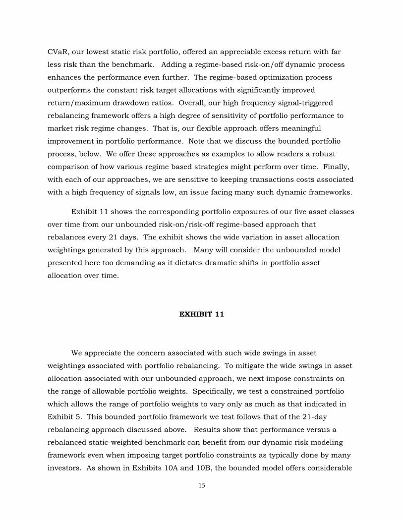
To generate the time series of our 21 day look-ahead portfolio risk forecast, we
repeat the steps above and forecast the portfolio 95% CVaR under an expanding
window approach. To avoid look-ahead bias, we incorporate only that market
information available at the time the model forecast is generated. The result of our
risk forecast effort is shown in Exhibit 6 as represented by our 21-day forward
combined portfolio CVaR for the base portfolio. As can be seen from Exhibit 6, our
portfolio risk estimate is highly responsive to actual market dynamics.
EXHIBIT 5
EXHIBIT 6
Forecasting Market Risk Environments
In the next part of our framework, we estimate the probability that the market
environment is already in or about to enter a turbulent state and use this information
to inform our asset allocation decision. Here, our asset allocation is determined in
accordance with one of two possible states of the world; normal risk (normal
uncertainty: normal return volatility and correlations), and high risk (high uncertainty:
high volatility and correlations, low returns). The two market states are governed by a
forward transition probability forecast of CVaR derived earlier. Specifically, our CVaR
forecast is used as the regime variable to fit a two-state Markov Regime Switching

10
process [see Ang Bekaert 2002, 2004)]. In this way, our regimes correspond to
market dynamics and the non-normal return distributions characterizing markets
Exhibit 7 reveals the meaningful presence of a normal regime and an event
regime in our time-series forecast of market downside risk. This is evidenced by the
substantial change in both the mean and the standard deviation of our CVaR regime
variable. Over the estimation period, the high-risk, event regime shows an average 21-
day CVaR (95%) of -14.22% with a standard deviation of 5.69%, as compared to a
higher average CVaR of -6.12% with a lower standard deviation of 1.63% for the
normal regime.
EXHIBIT 7
In general, the Markov-Switching model we use seeks to more effectively
capture the dynamic volatility of the regime variable as compared to simple data
partitions based on arbitrary thresholds. To understand why this is so, consider that
if the prior CVaR estimate suggests a high volatile (normal) state, the model would
more likely predict that the current market environment is also a high volatile (normal)
state. A naïve, fixed threshold may not make the same association and may thus
classify the current state as part of the normal regime, if the current CVaR value is
below the arbitrarily chosen threshold. In short, the regime model we employ is better
equipped to adapt over time to changing market conditions in real time.
Exhibit 8 shows the time-series results of the resulting forecast of the
probability that the markets are in, or about to be in, a high risk state (regime
probability bigger than 50%) over time. To estimate our model, we use an expanding
window approach with our first estimate in January 3, 2000 using data from February
1, 1996 to January 2, 2000. We generate each new forecast daily by simply adding
new observations and re-estimating the model with the new observations as the data
become available. The results, shown in Exhibit 8, Panel A, highlight that our
Markov-Switching model succeeded in meaningfully partitioning the market into two

11
regimes. Exhibit 8, Panel B, shows the specific dates identified as the market being in
a high-risk ―event‖ regime defined as an event probability of at least 50%.
EXHIBIT 8
A further understanding of the impact of our regime risk model on asset class
performance can be inferred from the data presented in Exhibit 9. Here, we
summarize the risk and return statistics for each of our five asset classes during the
study period, January 3, 2000 to October 10, 2011. A comparison of Exhibit 9A
(event days) and Exhibit 9B (full period), shows that during the event periods the
median returns for all risky assets are lower and standard deviation of returns are all
higher, versus the full period. These results suggest that the model assisted in
anticipating turbulent periods.4 Furthermore, extreme returns are shown to be a
dominant presence during forecasted event regimes. This can be seen from the
percentiles, e.g. the 5th percentile and 95th percentile are much further apart for the
event regime daily return distributions versus the full period.
EXHIBIT 9
Dynamic Asset Allocation
We now discuss the third, and final, part of our modeling; incorporating our
forecast of market turbulence into an effective dynamic asset allocation framework.
Our portfolio construction process responds to market dynamics by adjusting the
overall portfolio asset allocation in accordance with our regime-based risk forecast and
4 Furthermore, the maximum and minimum daily returns always occurred in the high volatile
event regime suggesting that investors might benefit from a regime model that can correctly
distinguish a third regime for high return periods.

12
Mean-CVaR optimization.5 As mentioned, we employ a risk-on (risk-off) approach as
driven by our model prediction for either a normal or high risk state, respectively.
Importantly, the dynamic portfolios we construct here facilitate a direct evaluation of
the risk present in markets with an eye towards mitigating the impact of abrupt
downside events frequenting markets via dynamic asset allocation.
Specifically, we solve equation 3 to obtain the weights of a portfolio that
maximizes expected return while targeting the CVaR to a desired level (see Rockafellar
and Uryasev [2002]). Expected returns and benchmark portfolio weights are shown in
Exhibit 5. This approach allows us to incorporate our copula-driven fat-tailed
simulation scenarios into a portfolio allocation optimization problem. Furthermore, as
we will see, this allows the optimal portfolio allocation to be determined in accordance
with our market regime prediction. Specifically, the fixed expected return vector is
represented by µ, and w is the set of weights that belongs to the space X. We examine
both an unconstrained portfolio with no-shorting and no-leverage portfolio (weights
must be between 0% and 100%) and a constrained portfolio with bounds as shown in
Exhibit 5. The CVaR target constraint is represented by and is the resulting
forward-looking CVaR at a 95% confidence level as estimated given the set of weights,
w, with a target CVaR level of γ.
(3)
We next demonstrate the approach by back-testing the model outcomes
combining all three parts of our process over time. We explore both unconstrained
and constrained portfolio weighting schemes as shown in Exhibit 5. As mentioned, we
reduce the effect of any hindsight bias on our results by using static, unadjusted
expected returns. The main focus of this paper is to show the meaningful impact that
can be had on portfolio performance by adjusting ―only‖ the portfolio asset allocation
in accordance with dynamic forecasts of market risk as captured by changing variance
and covariances across asset classes, over time. To this end, we forecast risk and
5 There is an extensive literature on advanced portfolio optimization techniques. See, for
instance, Fabozzi, et al., 2007 and Rachev, Stoyanov and Fabozzi 2008.

13
rebalance the portfolio according to pre-specified rules discussed below. For all
results, we use static expected returns and the policy portfolio as the benchmark
portfolio, as shown in Exhibit 5.
Exhibit 10 shows the results from our portfolio construction process. In Panel
A, we employ a set monthly rebalancing rule whereby we rebalance the portfolio every
21-days. We compare the performance of the benchmark portfolio to an unbounded
(weights must be between 0% and 100%, e.g., no shorting and no leverage) portfolio
construction processes, all rebalanced each 21 days. The two unbounded portfolios
are optimized portfolios based on CVaR, as discussed above. We show results for
several static target levels of CVaR, and we then allow the target level of CVaR to
switch over time between a high- and low-risk level in accordance with our dynamic
regime forecast.
In row 1 of Exhibit 10, Panel A, we show the performance of the benchmark
portfolio. We compare outcomes for our unbounded portfolios which allow for the
weights for each of our five asset classes to vary between 0% and 100% over the study
period. First, we show the performance of overall portfolios created by imposing a
series of constant, maximum allowable level of mean-CVaRs. Here, we report the
results for five constant target CVaR levels ranging from lowest risk (3 percent CVaR)
to highest risk (7 percent CVaR). This allows a comparison of how various CVaR limits
reflect changing risk conditions as estimated solely by our CVaR model, while
temporarily ignoring our market risk regime forecast in constructing portfolios. As
expected, portfolio draw downs and volatility rise with each higher level of allowable
risk along with higher realized total returns. Importantly, all mean-CVaR optimized
portfolios provide improved risk/return profiles, each outperforming the benchmark
portfolio showing positive alphas along with higher corresponding Sharpe ratios of
around 0.65.
EXHIBIT 10

14
Next, we add step 3 into our process by incorporating the signal derived from
our Markov-Switching risk model that identifies the current market state as being in
either a high-risk or low-risk environment. We estimate our model under the
expanding window approach with daily data beginning in February 1, 1996 with our
first regime risk estimate occurring in January 3, 2000. If the risk model output
suggests that the current environment is low-risk (high-risk) measured as less (more)
than a 50% likelihood of being in a high-risk state, then we implement a risk-on (risk-
off) strategy and optimize portfolio weights allowing for a CVaR risk target of 7% (3%),
respectively. As before, expected return assumptions are the same for each state, and
the optimization techniques are the same as those used in the constant target CVaR
process, above. The only difference being that we now allow the target portfolio to
change its risk profile to either risk-on (7% CVaR) or risk-off (3% CVaR) to reflect our
dynamic forecast of market risk.
In this approach, we simply use the same rebalancing conditions as the
constant CVaR process (i.e. same rebalancing dates and the constant 21-day
rebalancing period). On rebalancing days, we choose the target CVaR for the up-
coming 21-day period based on the prior day’s market risk regime signal. Results
show that incorporating the two-state market risk forecast meaningfully improves
results over the benchmark and the constant CVaR approach. With this risk-on/risk-
off framework, we are better able to capture a meaningful part of the upside that
markets have to offer while also reducing the downside. This approach represents
considerable improvement over the rebalanced, static benchmark and also the various
static levels of CVaR. As evidence, consider that for the risk on/off model the Sharpe
ratio rises to 0.68 while the maximum drawdown is now 19.73%, about half that of the
benchmark. We note that this max drawdown is equivalent to that calculated under
the 3% CVaR portfolio as calculated earlier but now captures much of the upside
afforded by the risk-on days.6
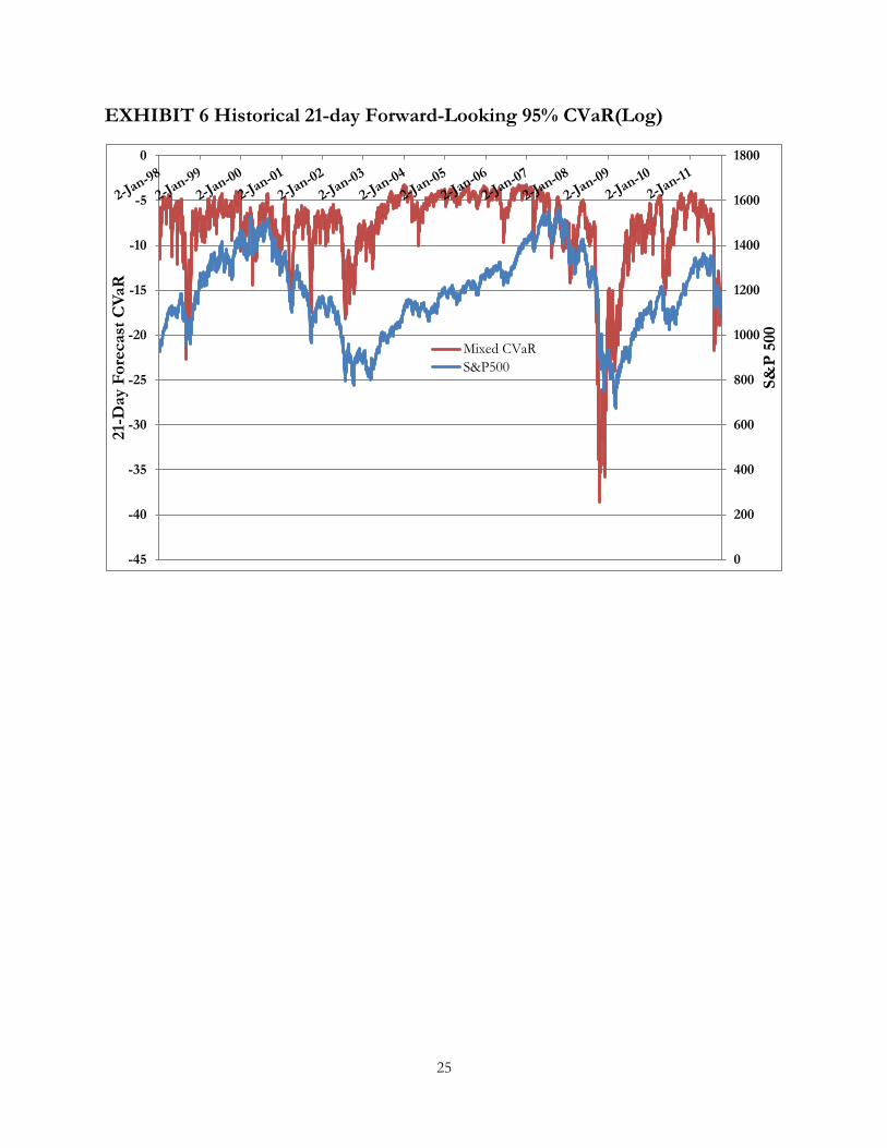
Exhibit 10B summarizes our results by plotting the risk-return relationships for
the various portfolios. Overall, results reflect the view that our CVaR tail risk
framework offers a highly relevant risk measurement approach for investors. All
CVaR related portfolios dominate the rebalanced static benchmark. Even the 3%
6 Our conclusions are unaffected when back-testing other rebalancing definitions.
15
CVaR, our lowest static risk portfolio, offered an appreciable excess return with far
less risk than the benchmark. Adding a regime-based risk-on/off dynamic process
enhances the performance even further. The regime-based optimization process
outperforms the constant risk target allocations with significantly improved
return/maximum drawdown ratios. Overall, our high frequency signal-triggered
rebalancing framework offers a high degree of sensitivity of portfolio performance to
market risk regime changes. That is, our flexible approach offers meaningful
improvement in portfolio performance. Note that we discuss the bounded portfolio
process, below. We offer these approaches as examples to allow readers a robust
comparison of how various regime based strategies might perform over time. Finally,
with each of our approaches, we are sensitive to keeping transactions costs associated
with a high frequency of signals low, an issue facing many such dynamic frameworks.
Exhibit 11 shows the corresponding portfolio exposures of our five asset classes
over time from our unbounded risk-on/risk-off regime-based approach that
rebalances every 21 days. The exhibit shows the wide variation in asset allocation
weightings generated by this approach. Many will consider the unbounded model
presented here too demanding as it dictates dramatic shifts in portfolio asset
allocation over time.
EXHIBIT 11
We appreciate the concern associated with such wide swings in asset
weightings associated with portfolio rebalancing. To mitigate the wide swings in asset
allocation associated with our unbounded approach, we next impose constraints on
the range of allowable portfolio weights. Specifically, we test a constrained portfolio
which allows the range of portfolio weights to vary only as much as that indicated in
Exhibit 5. This bounded portfolio framework we test follows that of the 21-day
rebalancing approach discussed above. Results show that performance versus a
rebalanced static-weighted benchmark can benefit from our dynamic risk modeling
framework even when imposing target portfolio constraints as typically done by many
investors. As shown in Exhibits 10A and 10B, the bounded model offers considerable

16
improvement in both risk and return versus the rebalanced static-benchmark.
Exhibit 12 shows the corresponding portfolio exposures over time for each of the five
asset classes associated with the bounded risk-on/risk-off regime-based approach.
As expected, it differs markedly from Exhibit 11. We note that during the global
financial crisis of 2008-2009, given the minimum allowable allocation to risky assets,
the model is unable to consistently achieve the desired 7% CVaR associated with a
risk-off regime. This simply means that we are not always able to obtain the portfolio
risk limits imposed when using a constrained approach with sizable minimum
allowable allocations to risky assets.
EXHIBIT 12
Exhibit 13 shows the total cumulative returns to the various rebalancing
approaches: benchmark, static allocations with 3%, 5% and 7% constant target CVaR,
and a regime-based allocation that switches between 3% and 7% target CVaR under
the same rebalancing conditions as the static allocations. This Exhibit offers visual
evidence that our regime-based risk framework offers investors a meaningful approach
to portfolio construction in the presence of fluctuating market risk.
Exhibit 13
Conclusions
We propose a dynamic portfolio construction model that accounts for the reality
of heavy tails and dynamic return correlations as witnessed in markets. The powerful
framework behind our portfolio construction is a dynamic process that integrates
high-frequency information to capture the time-varying risks of asset classes within
the investor’s portfolio. We use our dynamic risk information to adjust optimal asset
allocation across time and market states using only information known at the time of
model implementation. We find that ongoing monitoring of markets using our market

17
risk barometer and corresponding asset allocation framework offers investors the
promising opportunity to improve portfolio performance in challenging market
environments.
Acknowledgment
We thank Michael Barry, Xi Li, XXX, and the team at Georgetown University
Investment Office for their valuable comments and assistance.

18
References
Ang, A., and G. Bekaert. 2002. ―International Asset Allocation with Regime Shifts.‖ Review of Financial Studies, vol. 15, no. 4 (Fall):1137–1187. Ang, Andrew and Geert Bekaert. 2004. ―How Regimes Affect Asset Allocation.‖ Financial Analysts Journal, vol. 60, no. 2 (March/April):86–99. Black, Fischer. 1972. ―Capital Market Equilibrium with Restricted Borrowing.‖ The
Journal of Business, vol. 45, no. 3 (July):444–455.
Embrechts, Paul, Claudia Klüppelberg, and Thomas Mikosch. 1997. Modelling
Extremal Events for Insurance and Finance. Berlin/Heidelberg: Springer-Verlag.
Fabozzi, Frank J., Petter N. Kolm, Dessislava A. Pachamanova, Sergio M. Focardi . Robust Portfolio Optimization and Management. John Wiley & Sons. Hoboken, New Jersey, 2004.
Focardi, Sergio M. and Frank J. Fabozzi. 2004. The Mathematics of Financial Modeling
and Investment Management. Hoboken, NJ: John Wiley & Sons.
Glosten, Lawrence R., Ravi Jagannathan, and David E. Runkle. 1993. ―On the Relation between Expected Value and the Volatility of the Nominal Excess Return on
Stocks.‖ The Journal of Finance, vol. 48, no. 5 (December):1779–1801.
Hilal, Sawsan, Ser-Huang Poon, and Jonathan Tawn. 2011. ―Hedging the Black Swan:
Conditional Heteroskedasticity and Tail Dependence in S&P500 and VIX.‖ Journal of
Banking and Finance, vol. 35, no. 9 (September):2374–2387.
Hyung, Namwon, and Casper de Vries. 2007. ―Portfolio Selection with Heavy Tails.‖
Journal of Empirical Finance, vol. 14, no. 3 (June):383–400.
Kaya, Hakan, Wai Lee, and Bobby Pornrojnangkool. 2011. ―Implementable Tail Risk
Management: An Empirical Analysis of CVaR-Optimized Carry Trade Portfolios.‖
Journal of Derivatives & Hedge Funds, vol. 17, no. 4 (November):341–356.
Kritzman, Mark, Sebastien Page, and David A. Turkington. Forthcoming 2012.
―Regime Shifts: Implications for Dynamic Strategies.‖ Financial Analysts Journal.
Li, Xi, and Rodney N. Sullivan. 2011. ―A Dynamic Future for Active Quant Investing.‖
Journal of Portfolio Management, vol. 37, no. 3 (Spring):29–36.
McNeil, Alexander J., and Thomas Saladin. 1997. ―The Peaks over Thresholds Method
for Estimating High Quantiles of Loss Distributions.‖ Proceedings of 28th International
ASTIN Colloquium.
Rachev, Svetlozar T., Stoyan V. Stoyanov, and Frank J. Fabozzi. 2008. Advanced Stochastic Models, Risk Assessment, and Portfolio Optimization: The Ideal Risk,
Uncertainty, and Performance Measures. Hoboken, NJ: John Wiley & Sons.

19
Rockafellar, R. Tyrrell, and Stanislav Uryasev. ―Conditional Value-at-Risk for General
Loss Distributions.‖ Journal of Banking & Finance, vol. 26, no. 7 (July):1443–1471.
Sullivan, Rodney N., Steven P. Peterson, and David T. Waltenbaugh. 2010. ―Measuring
Global Systemic Risk: What Are Markets Saying about Risk?‖ Journal of Portfolio
Management, vol. 37, no. 1 (Fall):67–77.
Tsay, Ruey S. 2005. Analysis of Financial Time Series. Hoboken, NJ: John Wiley &
Sons.
Uryasev, Stanislav. 2000. ―Conditional Value-at-Risk: Optimization Algorithms and
Applications.‖ Financial Engineering News, no. 14 (February):1–5.
Xiong, James X., and Thomas M. Idzorek. 2011. ―The Impact of Skewness and Fat
Tails on the Asset Allocation Decision.‖ Financial Analysts Journal, vol. 67, no. 2
(March/April):23–35.
Xiong, James X., Roger G. Ibbotson, Thomas M. Idzorek, and Peng Chen. 2010. ―The
Equal Importance of Asset Allocation and Active Management.‖ Financial Analysts
Journal, vol. 66, no. 2 (March/April):22–30.

20
EXHIBIT 1 Asset Classes, Indices and Summary Statistics of Daily Returns
Period from February 1, 1996 to October 10, 2011
Global Equity Commodities Real Estate High Yield Investment Grade
Index MSCI ACWI SPGSCI DW REITs MLHY Barclay Agg
Mean 0.02% 0.03% 0.06% 0.03% 0.02%
Std Deviation 1.04% 1.50% 1.90% 0.29% 0.26%
Median 0.07% 0.03% 0.03% 0.05% 0.03%
Min -7.10% -8.76% -19.76% -4.73% -2.04%
Max 9.31% 7.48% 18.98% 2.78% 1.71%
1st Percentile -2.98% -4.08% -6.30% -0.87% -0.64%
99th Percentile
2.68% 3.62% 6.24% 0.73% 0.66%
5th Percentile -1.61% -2.40% -2.32% -0.36% -0.40%
95th Percentile
1.53% 2.37% 2.16% 0.36% 0.41%
10th Percentile -1.09% -1.70% -1.33% -0.21% -0.27%
90th Percentile
1.07% 1.82% 1.39% 0.24% 0.32%
Skewness -0.24 -0.16 0.44 -2.74 -0.27
Kurtosis 7.50 2.38 21.21 42.55 3.11

21
EXHIBIT 2 Autocorrelations of Daily Returns and Squared Returns – ACWI
Panel A. Log Daily Returns
Panel B. Standardized Log Residual Returns

22
EXHIBIT 3 ACWI Lower and Upper Tail Fit

23
EXHIBIT 4 Scatter Plot of ACWI vs GSCI Log Daily Returns

24
EXHIBIT 5 Portfolio Assumptions
Global Equity Commodities Real Estate High Yield Investment Grade
Index (MSCI ACWI) (SPGSCI) (DW REITs) (MLHY) (Barclay Agg)
Policy Allocation
45% 10% 10% 15% 20%
Portfolio Bounds
30 - 70% 5 - 15% 5 - 15% 7 - 23% 10 - 40%
Expected Returns
7% 6.5% 7% 6% 4%
25
EXHIBIT 6 Historical 21-day Forward-Looking 95% CVaR(Log)
0
200
400
600
800
1000
1200
1400
1600
1800
-45
-40
-35
-30
-25
-20
-15
-10
-5
0
S&
P 5
00
21-
Day F
ore
cast
CV
aR
Mixed CVaR
S&P500

26
EXHIBIT 7 Markov-Switching Model Perfect Insights Estimation
Regime 1
Regime 2 ("event")
Persistence Mu Sigma Persistence Mu Sigma
Market Downside Risk 99.14% -6.12% 1.63% 96.29% -14.22% 5.69%

27
EXHIBIT 8 Expanding Window Approach 1/3/2000 – 10/10/2011
(A) Probability of the Event Regime
0
0.5
1
0
200
400
600
800
1000
1200
1400
1600
1800
3-Jan-00 3-Jan-02 3-Jan-04 3-Jan-06 3-Jan-08 3-Jan-10
S&P500

28
EXHIBIT 8 Expanding Window Approach 1/3/2000 – 10/10/2011
(B) Event Regime Periods
Start 4-Jan-00 9-Feb-00 18-Feb-00 14-Apr-00 11-Oct-00 10-Nov-00 20-Feb-01 9-Mar-01 6-Jul-01 6-Sep-01
End 8-Feb-00 10-Feb-00 23-Feb-00 9-Jun-00 6-Nov-00 18-Jan-01 6-Mar-01 9-May-01 17-Jul-01 24-Oct-01
Trading Days in Between 24 1 2 38 18 45 10 42 7 31
Start 29-Oct-01 10-Dec-01 13-Dec-01 29-Jan-02 19-Feb-02 26-Jun-02 26-Nov-02 5-Dec-02 9-Dec-02 27-Dec-02
End 8-Nov-01 11-Dec-01 21-Dec-01 13-Feb-02 26-Feb-02 21-Nov-02 27-Nov-02 6-Dec-02 26-Dec-02 2-Jan-03
Trading Days in Between 8 1 6 11 5 104 1 1 12 3
Start 21-Jan-03 24-Jan-03 24-Feb-03 10-Mar-03 24-Mar-03 10-May-04 19-May-06 2-Jun-06 6-Jun-06 6-Jul-06
End 23-Jan-03 21-Feb-03 28-Feb-03 19-Mar-03 15-Apr-03 25-May-04 23-May-06 5-Jun-06 30-Jun-06 7-Jul-06
Trading Days in Between 2 19 4 7 16 11 2 1 18 1
Start 21-Jul-06 25-Jul-06 27-Feb-07 7-Jun-07 12-Jun-07 26-Jul-07 19-Oct-07 9-May-08 6-Jun-08 27-Jul-09
End 24-Jul-06 26-Jul-06 30-Mar-07 8-Jun-07 15-Jun-07 1-Oct-07 2-May-08 12-May-08 24-Jul-09 28-Jul-09
Trading Days in Between 1 1 23 1 3 46 134 1 285 1
Start 17-Aug-09 3-Sep-09 9-Sep-09 30-Oct-09 27-Nov-09 4-Feb-10 4-May-10 18-Mar-11 4-Aug-11
End 2-Sep-09 4-Sep-09 10-Sep-09 12-Nov-09 9-Dec-09 17-Feb-10 26-Jul-10 21-Mar-11 10-Oct-11
Trading Days in Between 12 1 1 9 8 8 57 1 46

29
EXHIBIT 9 Summary Statistics of Daily Returns 1/3/2000 – 10/10/2011
Global Equity Commodities Real Estate High Yield Investment Grade
Index MSCI ACWI SPGSCI DW REITs MLHY Barclay Agg
Mean 0.01% -0.02% 0.05% 0.00% 0.03%
Std Deviation 1.59% 1.89% 3.32% 0.47% 0.30%
Median 0.08% 0.03% 0.03% 0.03% 0.04%
Min -7.10% -8.76% -19.76% -4.73% -2.04%
Max 9.31% 7.48% 18.98% 2.78% 1.71%
1st Percentile -4.90% -5.35% -9.27% -1.62% -0.70%
99th Percentile 4.41% 4.93% 11.12% 1.12% 0.79%
5th Percentile -2.50% -3.13% -5.31% -0.74% -0.47%
95th Percentile 2.31% 2.81% 5.00% 0.64% 0.47%
10th Percentile -1.75% -2.26% -3.00% -0.46% -0.34%
90th Percentile 1.66% 2.12% 3.17% 0.44% 0.37%
Skewness -0.14 -0.28 0.33 -1.45 -0.18
Kurtosis 6.50 5.13 9.66 17.79 6.53
(A) Event Days
MSCI ACWI SPGSCI DW REITs MLHY Barclay Agg
Mean 0.01% 0.03% 0.07% 0.03% 0.03%
Std Deviation 1.13% 1.62% 2.20% 0.33% 0.26%
Median 0.07% 0.05% 0.09% 0.05% 0.03%
Min -7.10% -8.76% -19.76% -4.73% -2.04%
Max 9.31% 7.48% 18.98% 2.78% 1.71%
1st Percentile -3.55% -4.37% -7.37% -0.96% -0.64%
99th Percentile 2.90% 3.84% 7.33% 0.84% 0.66%
5th Percentile -1.74% -2.62% -2.88% -0.42% -0.41%
95th Percentile 1.61% 2.54% 2.61% 0.42% 0.42%
10th Percentile -1.21% -1.86% -1.71% -0.25% -0.28%
90th Percentile 1.14% 2.00% 1.65% 0.28% 0.33%
Skewness -0.21 -0.19 0.38 -2.51 -0.21
Kurtosis 9.86 5.02 18.63 38.30 6.13
(B) Full Period

EXHIBIT 10 Panel A Unbounded
Optimization
Info Ratio Alpha
Tracking Error
Sharpe Ratio
Return /
MaxDD MaxDD
Worst 21day loss
Annual Return
Annual Volatility
Hit Ratio
Benchmark
0.24 0.11 42.83% 15.99% 4.84% 14.26%
No leverage, no shorting Constant Target CVaR
3% 0.23 2.91% 12.56% 0.67 0.39 19.73% 13.00% 7.75% 8.32% 49.65%
4% 0.48 4.25% 8.78% 0.67 0.33 27.62% 15.52% 9.09% 10.56% 53.90%
5% 0.65 4.81% 7.36% 0.63 0.29 33.22% 16.34% 9.65% 12.45% 56.03%
6% 0.78 5.47% 7.05% 0.61 0.27 37.71% 16.97% 10.31% 14.11% 65.96%
7% 0.79 5.68% 7.20% 0.59 0.26 40.90% 17.53% 10.52% 15.29% 63.83%
Regime Based Target CVaR (Same Rebalancing Conditions)
3%, 7% 0.44 4.90% 11.09% 0.68 0.49 19.73% 14.84% 9.74% 11.39% 60.28%
Panel B Bounded Optimization Regime Based Target CVaR (Same Rebalancing Conditions)
Info Ratio Alpha TrackingError
Sharpe Ratio
Return /
MaxDD MaxDD
Worst 21day loss
Annual Return
Annual Volatility
Hit Ratio
Bound 3%, 7% 0.37 1.40% 3.74% 0.37 0.18 35.36% 13.20% 6.24% 12.54% 59.57%
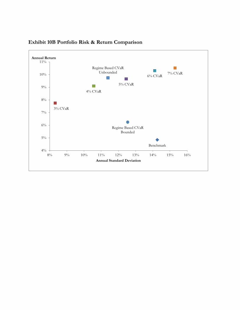
Exhibit 10B Portfolio Risk & Return Comparison
Benchmark
3% CVaR
4% CVaR
5% CVaR
6% CVaR 7% CVaR
Regime Based CVaR Unbounded
Regime Based CVaR Bounded
4%
5%
6%
7%
8%
9%
10%
11%
8% 9% 10% 11% 12% 13% 14% 15% 16%
Annual Return
Annual Standard Deviation
1
EXHIBIT 11 Optimal Portfolio Weights: Regime Based (3%, 7% Target
CVaR)
0%
10%
20%
30%
40%
50%
60%
70%
80%
90%
100%
1/
1/
2000
6/
1/
2000
11/
1/
2000
4/
1/
2001
9/
1/
2001
2/
1/
2002
7/
1/
2002
12/
1/
2002
5/
1/
2003
10/
1/
2003
3/
1/
2004
8/
1/
2004
1/
1/
2005
6/
1/
2005
11/
1/
2005
4/
1/
2006
9/
1/
2006
2/
1/
2007
7/
1/
2007
12/
1/
2007
5/
1/
2008
10/
1/
2008
3/
1/
2009
8/
1/
2009
1/
1/
2010
6/
1/
2010
11/
1/
2010
4/
1/
2011
9/
1/
2011
Equity Commodities Real Estate High Yield Invest. Grade

2
EXHIBIT 12 Optimal Portfolio Weights: Bounded Portfolio
0%
10%
20%
30%
40%
50%
60%
70%
80%
90%
100%
1/
3/
2000
5/
3/
2000
8/
31/
2000
1/
2/
2001
5/
3/
2001
8/
31/
2001
1/
7/
2002
5/
8/
2002
9/
6/
2002
1/
7/
2003
5/
8/
2003
9/
8/
2003
1/
7/
2004
5/
7/
2004
9/
8/
2004
1/
6/
2005
5/
9/
2005
9/
7/
2005
1/
6/
2006
5/
9/
2006
9/
7/
2006
1/
8/
2007
5/
9/
2007
9/
7/
2007
1/
8/
2008
5/
8/
2008
9/
8/
2008
1/
7/
2009
5/
8/
2009
9/
8/
2009
1/
7/
2010
5/
10/
2010
9/
8/
2010
1/
6/
2011
5/
9/
2011
9/
7/
2011
Equity Commodities Real Estate High Yield Invest. Grade

3
EXHIBIT 13 Cumulative Portfolio Returns
0
0.5
1
1.5
2
2.5
3
3.5
4
4.5 3% 5% 7% 3%-7% Benchmark