at SciVerse ScienceDirect

Energy 50 (2013) 74e82

Contents lists available

Energy

journal homepage: www.elsevier .com/locate/energy

Risk based multiobjective generation expansion planning consideringrenewable energy sources

Mohsen Gitizadeh*, Mahdi Kaji, Jamshid AghaeiDepartment of Electronics and Electrical Engineering, Shiraz University of Technology, Shiraz, Iran

a r t i c l e i n f o

Article history:Received 23 May 2012Received in revised form27 November 2012Accepted 29 November 2012Available online 3 January 2013

Keywords:Generation expansion planning (GEP)Renewable energy sources (RESs)Multiobjective optimizationModified normal boundary intersection(MNBI)Green certificate

* Corresponding author. Tel.: þ98 711 7264121; faxE-mail address: gitizadeh@sutech.ac.ir (M. Gitizad

0360-5442/$ e see front matter � 2012 Elsevier Ltd.http://dx.doi.org/10.1016/j.energy.2012.11.040

a b s t r a c t

Generation expansion planning is defined as the problem of finding the technology type, number ofgeneration units, size, and location of candidate plants within the planning horizon. In the deregulatedenvironment rather than the traditional system which considered the cost minimization as the mainobjective function in generation expansion planning problem, the major objective is to maximize theProject Lifetime Economic Return. In this paper, the problem is solved considering three objectives,simultaneously (i.e. maximization of the Project Lifetime Economic Return, minimization of CO2 emis-sion, and minimization of the fuel price risk due to the use of non-renewable energy sources).Furthermore, due to the extensive use of renewable energy sources, e.g., onshore wind, offshore wind,solar, etc, the effect of these power plants has been investigated in this paper. In order to make theproblem more compatible with the real world, some of the most common incentive systems (i.e. carbontax, emission trade, quota obligation, and feed-in-tariff) have been considered for the problem formu-lation. The problem is solved using Modified Normal Boundary Intersection method using GeneralAlgebraic Modelling System. Finally, a case study is designed to assess the efficiency of the proposedscheme.

� 2012 Elsevier Ltd. All rights reserved.

1. Introduction

The generation expansion planning (GEP) has historicallyaddressed the problem of determining what generation technologyto be commissioned, when the units to commit online, and wherethe units to be installed. By the time the electricity industrythroughout the world was mainly dominated by verticallyintegrated utilities, the main objective of GEP was to minimize thetotal cost (including investment and operating cost), to meet theexpected demand growth. After mid-1980 by liberalization ofthe electricity industry, energy producers had no more open accessto the grid and had a competitionwith other Generating Companies(GENCOs) to sell their produced energy. In this case, for a price takerGENCO, it is not guaranteed that its cost be covered and thus, themain objective of the GENCO would be maximizing the ProjectLifetime Economic Return (PLER) rather than minimizing the cost.

As it was mentioned, GEP is one of the earliest problems inpower systems industry and numerous techniques have beenapplied to solve the problem. In Ref. [1] dynamic programming and

: þ98 711 7353502.eh).

All rights reserved.

in Ref. [2,3] linear programing were used to solve the problem. InRef. [4] the Wien Automatic System Planning (WASP) is used tosolve GEP problem minimizing the cost of plan.

More recently the problem has solved by means of artificialintelligent methods. Chuang et al. used genetic algorithms inRef. [5]. In Ref. [6], the Evolutionary Programing (EP) techniquewith Gaussian mutation is used, and in Refs. [7e11] Particle SwarmOptimization (PSO), Simulated Annealing (SA), Tabu Search (TS),Ant Colony Optimization (ACO), and Genetic Algorithm (GA) areapplied to solve the GEP problem.

The electricity industry is one of the most important parts of thecountries’ economy and is a significant source of greenhouse gasemissions. Moreover, its economic and environmental role isgrowing in coming years. On the other hand, over the past decades,the demand for electricity has steadily increased and is expected torise in the upcoming years. Thus, many governments around theworld have worked on the issue of global warming and environ-mental protection. As the result they have agreed to Kyoto protocol[12,13], which commits the countries to reduce their greenhousegas emissions. In Ref. [12] and [13], in order to cope with Kyotoprotocol, the level of CO2 emission is considered as a constraint inGEP formulation. Nelson et al. [14] has carried out the powersystem planning by considering various CO2 pricing scenarios

Nomenclature

Indicest index corresponding to years of the planning horizonn index corresponding to a generation technology

available for planning

ConstantsT number of years in the planning horizond discount factor (rate of return) per-unit time on

investmentIn,t investment cost(V/MW) for the installation of

a generating unit of technology n in the tth yearpet average price of electrical energy in the tth year

(V/MWh)pgct green certificate price in the tth year (V/MWh)

εCO2n rate of CO2 emission releasing by the nth generating

unit (ton/MWh)Eoldn;t maximum energy (MWh) that can be produced in the

tth year by the set of units already installed in the year0, belonging to technology n.

FTn,t feed-in tariff for technology n in the tth yearPn rated power of generation units based on technology n

Sk,t expected coefficient of variation in prices of the fueltype k in period t

at percentage of energy produced and must be balancedby green certificates in the tth year

hgcn coefficient for assigning the green certificates to therenewable technology n corresponding to 1-MWhgeneration

ufn,t utilization factor

VariablesEst amount of energy sold in the tth year (MWh)Eexn;t amount of energy produced by the existing units

(MWh)Enewn;t amount of energy produced by the new generating

units (MWh)Un,t number of selected plants in the tth yearun,t number of units based on technology n benefiting from

renewable energy incentives in year tGstðGb

t Þ tradable Green Certificate (TGC) sold (bought) in thetth year

SetsNex set of existing generating unitsNnew set of candidate unitsJk set of unit fuel types

M. Gitizadeh et al. / Energy 50 (2013) 74e82 75

in order to make the planner use renewable energy sources. Careriet al. [15] have modelled several incentive systems to evaluate theirapplication effect in the age of green economy.

To the best of our knowledge, the contributions of this paperwith respect to the previous researches in the area can be listed asfollows:

(i) The generation expansion planning problem is solved usinga multiobjective mixed integer linear optimization model bya GENCO in the restructured power system. The proposedoptimization framework includes maximization of the GEN-CO’s PLER, minimization of CO2 emission, and maximization ofthe energy price risk. In addition, a simple risk model has beenimplemented that can quickly and efficiently evaluate the fuelprice volatility for the GEP problem.

(ii) Renewable Energy Sources (RESs) have been considered in theproposed GEP problem. Also, to motivate GENCOs to employthese kinds of technologies, financial incentives have beenimplemented in the proposed framework including feed-intariffs and green certificate trading schemes.

(iii) In the conventional multiobjective optimization methods, therange of the objective functions constructed based on thepayoff table may not be optimized. Consequently, it is notguaranteed the resulting Pareto set be an efficient or non-dominated Pareto set. Therefore, the lexicographic optimiza-tion is proposed here to calculate the payoff matrix to be usedin the NBI method. Accordingly, the Pareto optimal solutionsof Multiobjective Generation Expansion Planning (MOGEP) areidentified using the Modified Normal Boundary Intersection(MNBI) method.

The model is implemented in the General Algebraic ModellingSystem (GAMS), using CPLEX solver and applied to a hypotheticalGENCO [15].

The reminder of this paper has been organized as follows: InSection 2, the mathematical multiobjective generation expansionplanning problem formulation is introduced in the form of a Mixed

Integer Linear Programming (MILP). Section 3 introduces a frame-work based on NBI method to solve the multiobjective problem. InSection 4 simulation results are presented and the results obtainedby the application of the methodology are thoroughly discussed tohighlight the efficacy of the proposed approach. Some relevantconclusions are drawn in Section 5.

2. Multiobjective generation expansion planning problemformulation

RESs decrease the pollution production rates; contribute to theattainment of the Kyoto Protocol climate change mitigation goals,permit countries to develop security of energy supply bydecreasing fossil fuel dependency and offer several socioeconomicopportunities such as investment, development and job creation.

The model presented here, includes several RESs and CO2reduction measures. In this model three objectives are optimized inthe viewpoint of a GENCO, while the previous models mostlyconsider only one objective. In comparison with single objectiveoptimization techniques, the Pareto-based multiobjective optimi-zation methods have a number of advantages including the abilityof having enough flexibility to deal with conflicting objectives [16].

2.1. Objective functions

2.1.1. Maximization of PLERThis objective function is defined as the overall present value

sum of revenues minus the total present value of costs.

f1¼Xt˛T

ð1þdÞ1�t

264pet E

st�

Pn˛Nex

lnEexn;tþP

n˛Nnew

�Ftn;t�ln

�Enewn;t

� Pn˛Nnew

In;tUn;tPnþpgct

�Gst�Gb

t

�375 (1)

In this formulation, FTn,t represents the feed-in tariff for tech-nology n in the tth year of the planning horizon. A feed-in tariff isa policy mechanism designed to speed up investment in renewableenergy technologies. This aim can be attained by offering long-term

M. Gitizadeh et al. / Energy 50 (2013) 74e8276

contracts to renewable energy producers, classically based uponthe cost of generation of each technology [17]. Besides, Gs

tðGbt Þis the

Tradable Green Certificate (TGC) sold (bought) in the tth year. Greentags or green certificates stand for cost-efficient tools to stimulateelectricity production from RESs. These certificates can be traded orused, and can be sold together with the electrical energy or sepa-rately to it.

The other costs of each technology are considered asmultiplyingthe amount of produced energy by l. This coefficient is variable costof per-unit of energywhich is as the variable unit cost (per MWh) ofa payment stream that has the same present value as the total costof building a generating plant over its life. Here it includesdecommissioning costs (Dn,t), fuel costs (Fn,t), and maintenancecosts (Mn,t) as follows [15]:

ln ¼

PTt¼1

Dn;t þ Fn;t þMn;t

ð1þ dÞt�1PTt¼1

En;tð1þ dÞt�1

for all n: (2)

2.1.2. Minimization of environmental impactsDespite the previously mentioned benefits, renewable energy

competes with conventional electricity on an imbalanced playingfield amid a failure to internalize the negative externalities asso-ciated with conventional energy production. In other words, inorder to make the applications of RES more justifiable, the partyresponsible for environmental pollution (e.g. air pollution) must bein charge of paying for the negative impacts caused. In this case, it issaid that the external costs have been internalized and thus, themarket mechanism will not fail to secure an optimal allocation ofresources.

Furthermore, the carbon dioxide emissions from fossil-fuelplants should be minimized because of their danger for the globalwarming (greenhouse). Therefore, the second objective is consid-ered as the minimization of the environmental effects byminimizing

f2 ¼Xt˛T

" Xn˛Nex

εCO2n Eexn;t þ

Xn˛Nnew

εCO2n Enewn;t

#(3)

Moreover, more polluting gases such as NOx and SOx can beconsidered if necessary. It should be noted that by minimizing CO2emission, the released NOx and SOx will be minimized.

2.1.3. Minimization of energy price risk (volatility)A key feature in the price of the electrical energy is the fuel price

in conventional energy sources. Fuel price changes dramaticallydue to numerous reasons over time and thus, it is desired fora GENCO to control the risk of employing units using different typesof fuels. The following equation contributes the vulnerability ofenergy price changes to the expansion plan model. More specifi-cally using this equation the fuel price volatility is to be minimized.

f3 ¼Xt˛T

24Xk˛F

Sk;tXn˛Jk

EFn;t

35 (4)

This riskmeasure in prices is simple but original inmultiobjectivemodels [18].

2.2. Constraints

In this multiobjective problem nine sets of constraints havebeen applied as described below.

2.2.1. Energy balanceThis equality constraint shows the balance between the amount

of energy by all units (existing as well as new ones) and energy soldat the market in year t.

Est ¼Xn˛Nex

Eexn;t þX

n˛Nnew

Enewn;t (5)

2.2.2. Sold energy constraintsThe amount of energy that the GENCO wants to sell at the

market is limited by proper bounds as follows.

Est min � Est � Est max (6)

2.2.3. Quota obligationThis constraint stands for themechanism of the quota obligation

for RESs. This obligation forces the electricity supply companies toproduce a specific part of their energy from RESs. Furthermore,their green certificate will be tradable, and each GENCO can buy orsell its right to other GENCOs upon its needs.

Xk˛F

at

Enewk þ Eexk

!¼ Gb

t � Gst þ

Xn˛Nnew

hgcn Enewn;t (7)

The right hand side of Eq. (7) is a specific fraction of the totalproduced energy from conventional sources, which must bebalanced with the green certificate bought (sold) Gb

t ðGstÞ and

produced energy from renewable energy sources.

2.2.4. Generation limitsEnergy output of the units should be limited by the following

inequalities:

Enewn;t � 8760� ufn;tun;tPn;t (8)

Eexn;t � 8760� ufn;tPn;t�Un;t � un;t

�þ E

oldn;t (9)

In Eq. (9) un,t > 0 by the time the incentive period is not expired.After that, the unit is shifted from new units to existing ones.

2.2.5. Maximum construction timeThese physical constraints reflect the maximum number of

yearly construction capability of various types of units to becommitted in the planning horizon.

0 � Un;t � Un;t (10)

0 � un;t � un;t (11)

2.2.6. Maximum investment limitThis economic constraint stands for the maximum amount of

investment which will be made by the GENCO.

XTt¼1

ð1þ dÞ1�t

" Xn˛Snew

In;tPnUn;t

#� Imax (12)

2.2.7. Non-negativity constraintsThe following variable should be positive in the problem.

Gbt ;G

st ;Un;t ;un;t ; Est ; E

newn;t ; Eexn;t � 0 (13)

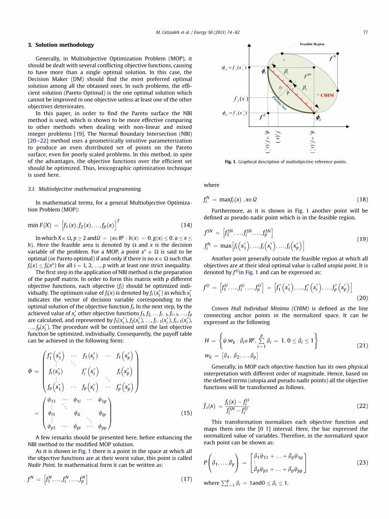
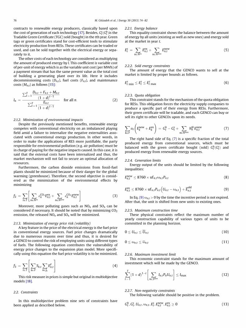
Fig. 1. Graphical description of multiobjective reference points.

M. Gitizadeh et al. / Energy 50 (2013) 74e82 77

3. Solution methodology

Generally, in Multiobjective Optimization Problem (MOP), itshould be dealt with several conflicting objective functions, causingto have more than a single optimal solution. In this case, theDecision Maker (DM) should find the most preferred optimalsolution among all the obtained ones. In such problems, the effi-cient solution (Pareto Optimal) is the one optimal solution whichcannot be improved in one objective unless at least one of the otherobjectives deteriorates.

In this paper, in order to find the Pareto surface the NBImethod is used, which is shown to be more effective comparingto other methods when dealing with non-linear and mixedinteger problems [19]. The Normal Boundary Intersection (NBI)[20e22] method uses a geometrically intuitive parameterizationto produce an even distributed set of points on the Paretosurface, even for poorly scaled problems. In this method, in spiteof the advantages, the objective functions over the efficient setshould be optimized. Thus, lexicographic optimization techniqueis used here.

3.1. Multiobjective mathematical programming

In mathematical terms, for a general Multiobjective Optimiza-tion Problem (MOP):

min F�X� ¼

hf1�x�; f2�x�;.; fp

�x�iT

(14)

Inwhich X˛U, p� 2 andU ¼ fx˛Rp : hðxÞ ¼ 0; gðxÞ � 0; a� x�bg. Here the feasible area is denoted by U and x is the decisionvariable of the problem. For a MOP, a point x* ˛ U is said to beoptimal (or Pareto optimal) if and only if there is no x ˛ U such thatfi(x) � fi(x*) for all i ¼ 1, 2, ., p with at least one strict inequality.

The first step in the application of NBI method is the preparationof the payoff matrix. In order to form this matrix with p differentobjective functions, each objective (fi) should be optimized indi-vidually. The optimum value of fi(x) is denoted by fi (x*i ) in which x*iindicates the vector of decision variable corresponding to theoptimal solution of the objective function fi. In the next step, by theachieved value of x*i other objective functions f1, f2, . fi�1, fiþ1,., fpare calculated, and represented by f1(x*i ), f2(x

*i ), ., fi�1(x*i ), fiþ1(x*i ),

., fp(x*i ). The procedure will be continued until the last objectivefunction be optimized, individually. Consequently, the payoff tablecan be achieved in the following form:

F ¼

0BBBBBBB@

f *1�x*1�

/ f1�x*i�

/ f1�x*p�

« 1

fi�x*1�

f *i�x*i�

fi�x*p�

« 1

fp�x*1�

/ fp�x*i�

/ f *p�x*p�

1CCCCCCCA

¼

0BBBB@f11 / f1i / f1p« 1fi1 fii fip« 1

fp1 / fpi / fpp

1CCCCA (15)

A few remarks should be presented here, before enhancing theNBI method to the modified MOP solution.

As it is shown in Fig. 1 there is a point in the space at which allthe objective functions are at their worst value, this point is calledNadir Point. In mathematical form it can be written as:

f N ¼hf N1 ;.; f Ni ;.; f Np

i(17)

where

f Ni ¼ maxfi�x�; x˛U (18)

Furthermore, as it is shown in Fig. 1 another point will bedefined as pseudo nadir point which is in the feasible region.

f SN ¼hf SN1 ;.; f SNi ;.; f SNp

if Ni ¼ max

hfi�x*1�;.; fi

�x*i�;.; fi

�x*p�i (19)

Another point generally outside the feasible region at which allobjectives are at their ideal optimal value is called utopia point. It isdenoted by f U in Fig. 1 and can be expressed as:

f U ¼hf U1 ;.; f Ui ;.; f Up

i¼hf *1�x*1�;.; f *i

�x*i�;.; f *p

�x*p�i

(20)

Convex Hull Individual Minima (CHIM) is defined as the lineconnecting anchor points in the normalized space. It can beexpressed as the following

H ¼(4:wk : bi˛Rp;

Ppi¼1

bi ¼ 1; 0 � bi � 1

)wk ¼ �

b1; b2;.; bp� (21)

Generally, in MOP each objective function has its own physicalinterpretation with different order of magnitude. Hence, based onthe defined terms (utopia and pseudo nadir points) all the objectivefunctions will be transformed as follows.

f i�x� ¼ fi

�x�� f Ui

f SNi � f Ui(22)

This transformation normalizes each objective function andmaps them into the [0 1] interval. Here, the bar expressed thenormalized value of variables. Therefore, in the normalized spaceeach point can be shown as:

P

0@b1;.; bp

1A ¼24 b1411 þ.þ bp41p«bp4p1 þ.þ bp4pp

35 (23)

wherePp

i¼1 bi ¼ 1and0 � bi � 1.

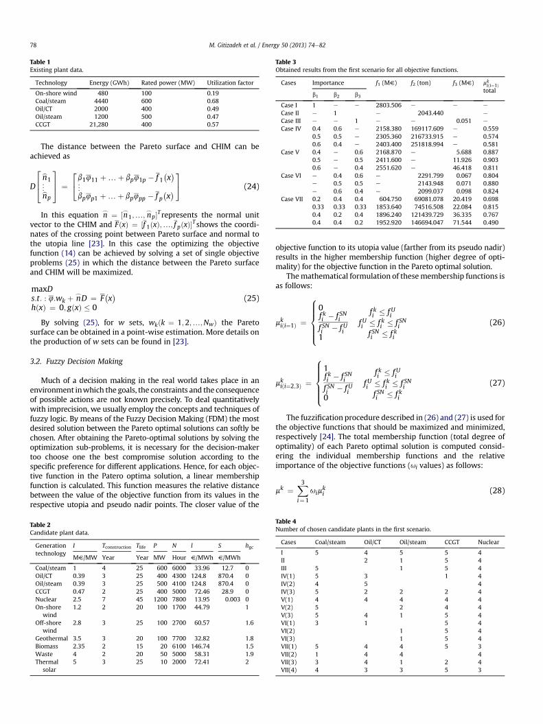
Table 1Existing plant data.

Technology Energy (GWh) Rated power (MW) Utilization factor

On-shore wind 480 100 0.19Coal/steam 4440 600 0.68Oil/CT 2000 400 0.49Oil/steam 1200 500 0.47CCGT 21,280 400 0.57

Table 3Obtained results from the first scenario for all objective functions.

Cases Importance f1 (MV) f2 (ton) f3 (MV) mkiði¼1Þtotal

b1 b2 b3

Case I 1 e e 2803.506 e e e

Case II e 1 e 2043.440 e

Case III e e 1 e e 0.051 e

Case IV 0.4 0.6 e 2158.380 169117.609 e 0.5590.5 0.5 e 2305.360 216733.915 e 0.5740.6 0.4 e 2403.400 251818.994 e 0.581

Case V 0.4 e 0.6 2168.870 e 5.688 0.8870.5 e 0.5 2411.600 e 11.926 0.9030.6 e 0.4 2551.620 e 46.418 0.811

Case VI e 0.4 0.6 e 2291.799 0.067 0.804e 0.5 0.5 e 2143.948 0.071 0.880e 0.6 0.4 e 2099.037 0.098 0.824

Case VII 0.2 0.4 0.4 604.750 69081.078 20.419 0.6980.33 0.33 0.33 1853.640 74516.508 22.084 0.8150.4 0.2 0.4 1896.240 121439.729 36.335 0.7670.4 0.4 0.2 1952.920 146694.047 71.544 0.490

M. Gitizadeh et al. / Energy 50 (2013) 74e8278

The distance between the Pareto surface and CHIM can beachieved as

D

264 bn1«bnp

375 ¼24b1411 þ.þ bp41p � f 1

�x�

«bp4p1 þ.þ bp4pp � f p

�x�35 (24)

In this equation n_ ¼ ½n_1;.; n

_p�Trepresents the normal unit

vector to the CHIM and FðxÞ ¼ ½f 1ðxÞ;.; f pðxÞ�Tshows the coordi-nates of the crossing point between Pareto surface and normal tothe utopia line [23]. In this case the optimizing the objectivefunction (14) can be achieved by solving a set of single objectiveproblems (25) in which the distance between the Pareto surfaceand CHIM will be maximized.

maxDs:t: : 4:wk þ n

_D ¼ F

�x�

hðxÞ ¼ 0; gðxÞ � 0(25)

By solving (25), for w sets, wkðk ¼ 1;2;.;NwÞ the Paretosurface can be obtained in a point-wise estimation. More details onthe production of w sets can be found in [23].

3.2. Fuzzy Decision Making

Much of a decision making in the real world takes place in anenvironment inwhich the goals, the constraints and the consequenceof possible actions are not known precisely. To deal quantitativelywith imprecision, we usually employ the concepts and techniques offuzzy logic. By means of the Fuzzy Decision Making (FDM) the mostdesired solution between the Pareto optimal solutions can softly bechosen. After obtaining the Pareto-optimal solutions by solving theoptimization sub-problems, it is necessary for the decision-makertoo choose one the best compromise solution according to thespecific preference for different applications. Hence, for each objec-tive function in the Patero optima solution, a linear membershipfunction is calculated. This function measures the relative distancebetween the value of the objective function from its values in therespective utopia and pseudo nadir points. The closer value of the

Table 2Candidate plant data.

Generationtechnology

I Tconstruction Tlife P N l S hgc

MV/MW Year Year MW Hour V/MWh V/MWh

Coal/steam 1 4 25 600 6000 33.96 12.7 0Oil/CT 0.39 3 25 400 4300 124.8 870.4 0Oil/steam 0.39 3 25 500 4100 124.8 870.4 0CCGT 0.47 2 25 400 5000 72.46 28.9 0Nuclear 2.5 7 45 1200 7800 13.95 0.003 0On-shore

wind1.2 2 20 100 1700 44.79 1

Off-shorewind

2.8 3 25 100 2700 60.57 1.6

Geothermal 3.5 3 20 100 7700 32.82 1.8Biomass 2.35 2 15 20 6100 146.74 1.5Waste 4 2 20 50 5000 58.31 1.9Thermal

solar5 3 25 10 2000 72.41 2

objective function to its utopia value (farther from its pseudo nadir)results in the higher membership function (higher degree of opti-mality) for the objective function in the Pareto optimal solution.

Themathematical formulation of thesemembership functions isas follows:

mkiði¼1Þ ¼

8>>>><>>>>:0f ki � f SNif SNi � f Ui1

f ki � f Uif Ui � f ki � f SNi

f SNi � f ki

(26)

mkiði¼2;3Þ ¼

8>>>><>>>>:1f ki � f SNif SNi � f Ui0

f ki � f Uif Ui � f ki � f SNi

f SNi � f ki

(27)

The fuzzification procedure described in (26) and (27) is used forthe objective functions that should be maximized and minimized,respectively [24]. The total membership function (total degree ofoptimality) of each Pareto optimal solution is computed consid-ering the individual membership functions and the relativeimportance of the objective functions (ui values) as follows:

mk ¼X3i¼1

uimki (28)

Table 4Number of chosen candidate plants in the first scenario.

Cases Coal/steam Oil/CT Oil/steam CCGT Nuclear

I 5 4 5 5 4II 2 1 5 4III 5 1 5 4IV(1) 5 3 1 4IV(2) 4 5 4IV(3) 5 2 2 2 4V(1) 4 4 4 4 4V(2) 5 2 4 4V(3) 5 4 1 5 4VI(1) 3 1 5 4VI(2) 1 5 4VI(3) 1 5 4VII(1) 5 4 4 5 3VII(2) 1 4 4 4VII(3) 3 4 1 2 4VII(4) 4 3 3 5 3

1600 1800 2000 2200 2400 2600 28000

1

2

3

4

5

6x 10

5

PLER (M€)

Em

issi

on (t

on)

Fig. 2. PLER and Emission Trade-off in the first scenario.

2000 2100 2200 2300 2400 2500 2600 2700 2800 29000.05

0.1

0.15

0.2

0.25

Emission (ton)

Ris

k (M

€)

Fig. 4. Emission and fuel price volatility (Risk) Trade-off in the first scenario.

M. Gitizadeh et al. / Energy 50 (2013) 74e82 79

The best planning scheme is determined by ranking theschemes based on value of mk which is represented in (28). In thispaper, the importance of objective functions is the same asw valueswhich was introduced in Eq. (25).

4. Simulation results and discussion

The proposed framework of the GEP problem is applied ona hypothetical GENCO for a 14-year planning horizon. The energymarket price is supposed to increase linearly from 90.1 V/MWh(year 2012) to 108.3 V/MWh (the last year of planning horizon).This price is considered to be deterministic and its stochastic natureis ignored in this study. As in [15], the annual price of greencertificates can be obtained bypgc

t ¼ 180� pet . The main charac-

teristics of the existing technologies are presented in Table 1 whichrepresents the initial conditions of the expansion plan [15]. Thetechnology of coal-fired power plant is super-critical pulverisedcoal (SCPC). In this table, the technology of Oil/CT power plant isbased on the combustion turbine and CCGT shows the combinedcycle gas turbine.

In order to calculate the present value of the first objectivefunction (i.e. PLER) a 5% discount rate is considered (r ¼ 0.05).Table 2 consists of 11 different types of plants including non-RESs(for instance, nuclear plant) and RES-based technologies [15].Here I is the capital cost of each technology, and l is the variable costof different candidate plants. P shows the rated power of generationunits based on technology n, Sk,t is the Expected coefficient of

0 500 1000 1500 2000 2500 30000

50

100

150

PLER (M€)

Ris

k (M

€)

Fig. 3. PLER and fuel price volatility (Risk) Trade-off in the first scenario.

variation in prices of the fuel type k in period t, and N is theutilization hours per year. In this table, coefficient hgc is to assigngreen certificate to renewable energy source to be compatible inthe market. The construction time of each plant is also consideredas a constraint in this problem.

To have better illustration of the proposed framework features,two scenarios have been studied in the following subsections.

4.1. Scenario I: GEP without considering RES-based technologies

In order to analyse the effects of RES-based technologies in theproposed MOGEP problem two scenarios are analysed here. In thisscenario, the candidates are coal, oil, combined cycle gas turbine,and nuclear power plants.

Using the MNBI method for the proposed formulation of theMOGEP, the payoff table obtained. According to the payoff table (F)the ideal and anti-ideal points of objective functions f1 to f3 isdetermined as the minimum and maximum values of rows 1 to 3,respectively.

F1 ¼24 2803:50 �473:08 �535:51506421:20 2043:44 2883:20

15:43 0:21 0:05

35The results of the first and third rows in terms of million euros

are related to the PLER and fuel price volatility (risk), and thesecond row in ton corresponds to the emission. The main diagonalof the payoff table F1 shows the result of the individual optimiza-tion of the objective functions (the utopia point).

-20000

20004000

6000

0

24

6

× 105

0

50

100

150

PLER (M€)Emission (ton)

Ris

k(M

€)

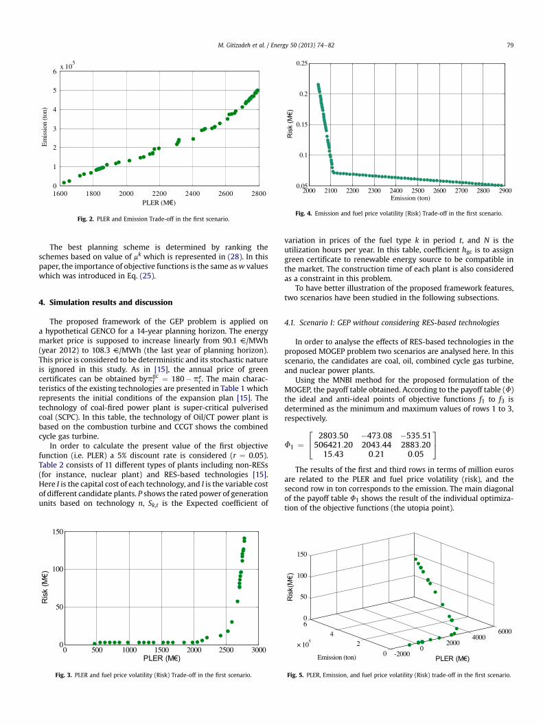
Fig. 5. PLER, Emission, and fuel price volatility (Risk) trade-off in the first scenario.

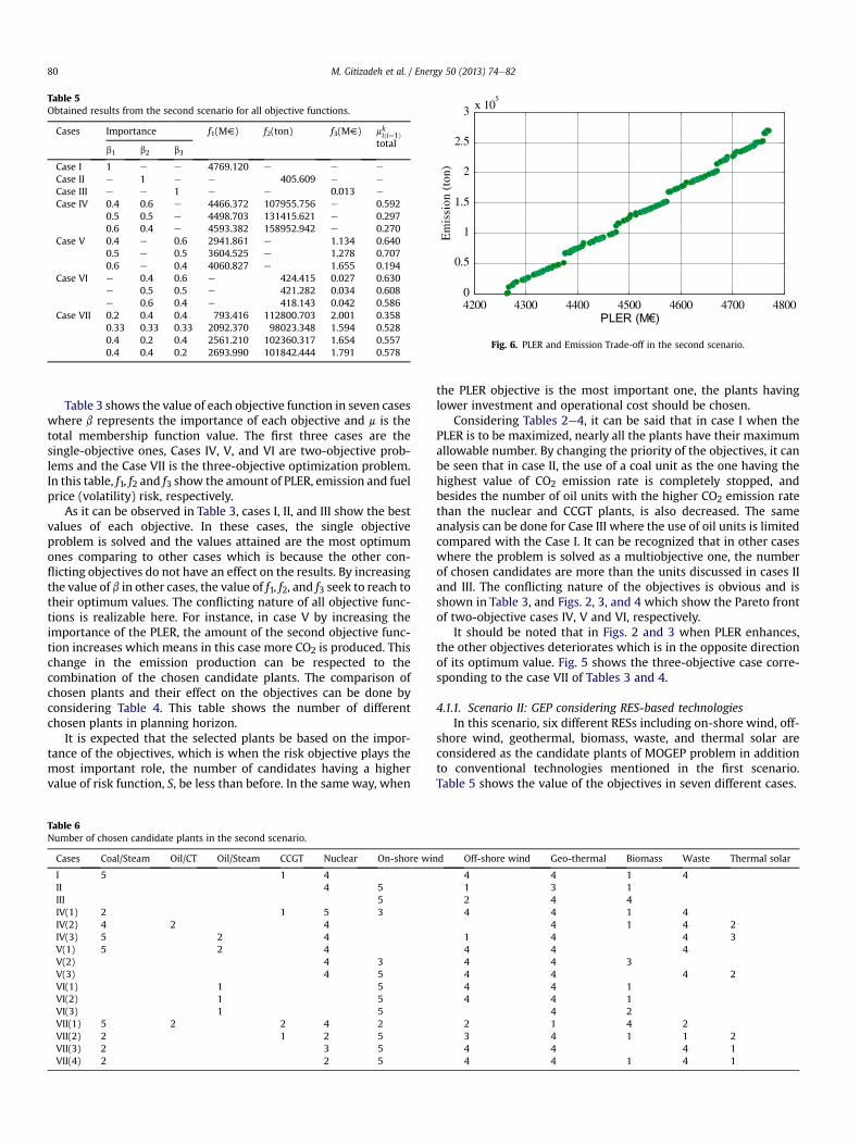
Table 5Obtained results from the second scenario for all objective functions.

Cases Importance f1(MV) f2(ton) f3(MV) mkiði¼1Þtotal

b1 b2 b3

Case I 1 e e 4769.120 e e e

Case II e 1 e e 405.609 e e

Case III e e 1 e e 0.013 e

Case IV 0.4 0.6 e 4466.372 107955.756 e 0.5920.5 0.5 e 4498.703 131415.621 e 0.2970.6 0.4 e 4593.382 158952.942 e 0.270

Case V 0.4 e 0.6 2941.861 e 1.134 0.6400.5 e 0.5 3604.525 e 1.278 0.7070.6 e 0.4 4060.827 e 1.655 0.194

Case VI e 0.4 0.6 e 424.415 0.027 0.630e 0.5 0.5 e 421.282 0.034 0.608e 0.6 0.4 e 418.143 0.042 0.586

Case VII 0.2 0.4 0.4 793.416 112800.703 2.001 0.3580.33 0.33 0.33 2092.370 98023.348 1.594 0.5280.4 0.2 0.4 2561.210 102360.317 1.654 0.5570.4 0.4 0.2 2693.990 101842.444 1.791 0.578

4200 4300 4400 4500 4600 4700 48000

0.5

1

1.5

2

2.5

3 x 105

PLER (M€)

Em

issi

on (

ton)

Fig. 6. PLER and Emission Trade-off in the second scenario.

M. Gitizadeh et al. / Energy 50 (2013) 74e8280

Table 3 shows the value of each objective function in seven caseswhere b represents the importance of each objective and m is thetotal membership function value. The first three cases are thesingle-objective ones, Cases IV, V, and VI are two-objective prob-lems and the Case VII is the three-objective optimization problem.In this table, f1, f2 and f3 show the amount of PLER, emission and fuelprice (volatility) risk, respectively.

As it can be observed in Table 3, cases I, II, and III show the bestvalues of each objective. In these cases, the single objectiveproblem is solved and the values attained are the most optimumones comparing to other cases which is because the other con-flicting objectives do not have an effect on the results. By increasingthe value of b in other cases, the value of f1, f2, and f3 seek to reach totheir optimum values. The conflicting nature of all objective func-tions is realizable here. For instance, in case V by increasing theimportance of the PLER, the amount of the second objective func-tion increases which means in this case more CO2 is produced. Thischange in the emission production can be respected to thecombination of the chosen candidate plants. The comparison ofchosen plants and their effect on the objectives can be done byconsidering Table 4. This table shows the number of differentchosen plants in planning horizon.

It is expected that the selected plants be based on the impor-tance of the objectives, which is when the risk objective plays themost important role, the number of candidates having a highervalue of risk function, S, be less than before. In the same way, when

Table 6Number of chosen candidate plants in the second scenario.

Cases Coal/Steam Oil/CT Oil/Steam CCGT Nuclear On-shore win

I 5 1 4II 4 5III 5IV(1) 2 1 5 3IV(2) 4 2 4IV(3) 5 2 4V(1) 5 2 4V(2) 4 3V(3) 4 5VI(1) 1 5VI(2) 1 5VI(3) 1 5VII(1) 5 2 2 4 2VII(2) 2 1 2 5VII(3) 2 3 5VII(4) 2 2 5

the PLER objective is the most important one, the plants havinglower investment and operational cost should be chosen.

Considering Tables 2e4, it can be said that in case I when thePLER is to be maximized, nearly all the plants have their maximumallowable number. By changing the priority of the objectives, it canbe seen that in case II, the use of a coal unit as the one having thehighest value of CO2 emission rate is completely stopped, andbesides the number of oil units with the higher CO2 emission ratethan the nuclear and CCGT plants, is also decreased. The sameanalysis can be done for Case III where the use of oil units is limitedcompared with the Case I. It can be recognized that in other caseswhere the problem is solved as a multiobjective one, the numberof chosen candidates are more than the units discussed in cases IIand III. The conflicting nature of the objectives is obvious and isshown in Table 3, and Figs. 2, 3, and 4 which show the Pareto frontof two-objective cases IV, V and VI, respectively.

It should be noted that in Figs. 2 and 3 when PLER enhances,the other objectives deteriorates which is in the opposite directionof its optimum value. Fig. 5 shows the three-objective case corre-sponding to the case VII of Tables 3 and 4.

4.1.1. Scenario II: GEP considering RES-based technologiesIn this scenario, six different RESs including on-shore wind, off-

shore wind, geothermal, biomass, waste, and thermal solar areconsidered as the candidate plants of MOGEP problem in additionto conventional technologies mentioned in the first scenario.Table 5 shows the value of the objectives in seven different cases.

d Off-shore wind Geo-thermal Biomass Waste Thermal solar

4 4 1 41 3 12 4 44 4 1 4

4 1 4 21 4 4 34 4 44 4 34 4 4 24 4 14 4 1

4 22 1 4 23 4 1 1 24 4 4 14 4 1 4 1

0 1000 2000 3000 4000 50000

0.5

1

1.5

2

2.5

PLER (M€)

Ris

k (M

€)

Fig. 7. PLER and fuel price volatility (Risk) Trade-off in the second scenario.

01000

20003000

40005000

01

23

× 105

0

2

4

6

PLER (M€)Emission (ton)

Ris

k (M

€)

Fig. 9. PLER, Emission, and fuel price volatility (Risk) trade-off in the first scenario.

M. Gitizadeh et al. / Energy 50 (2013) 74e82 81

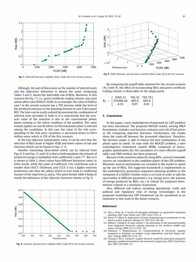
Although, the part of discussion on the number of selected unitsand the objectives’ behaviour is almost the same, comparingTables 3 and 5, shows the noticeable role of RESs. Moreover, in thisscenario the Eq. (7), i.e., green certificate trading scheme, was usedwhich affects the GENCO’s PLER. As an example, the value of PLER incase I in the second scenario has a 70% increase while the level ofthe produced emission in the planning horizon in case II decreased80%. The later can be easily realized by assessing the combination ofselected units provided in Table 6. It is noteworthy that the non-zero value of the emission is due to the conventional powerplants existing in the initial condition of the problem. The sameremark applies on case III where no thermal power plant is selectedamong the candidates. In this case the value of the risk corre-sponding to the fuel price variations is decreased down to 0.013million euros which is 25% of the first scenario.

In the two objective optimization cases, it can be seen that theselection of RESs leads to higher PLER and lower values of risk andemission which can be found in Figs. 2e9.

Another interesting observation which can be inferred fromFigs. 8, 9 and Eqs. (3) and (4) is that in both equations the amount ofproduced energy is multiplied with coefficients S and ε

CO2 . But as itis shown in Table 2, these values have different behaviour ratios. Inother words, while the value of coefficient S for Coal/Steam unit issmaller than Oil/CT, Oil/Steam, and CCGT, it has a higher emissionproduction rate than the others which in turn leads to conflictingmanner of the objectives f2 and f3. This point beside Table 6 helps toclarify the behaviour of the objective functions shown in Fig. 9.

405 410 415 420 425 430 435 440 4450.01

0.02

0.03

0.04

0.05

0.06

0.07

Emission (ton)

Ris

k (M

€)

Fig. 8. Emission and fuel price volatility (Risk) Trade-off in the second scenario.

By comparing the payoff table obtained for the second scenario(F2) with F1 the effect of incorporating RESs and green certificatetrading scheme is observable on the utopia point.

F2 ¼24 4769:12 792:35 792:70270360:24 405:6 445:6

4:33 0:07 0:01

35

5. Conclusions

In this paper, a new multiobjective framework for GEP problemhas been introduced. The proposed MOGEP model, owning MILPformulation, includes cost function, emission and risk of fuel pricesas the competing objective functions. Furthermore, the resultsshow the trade-off between the presented objectives. Therefore,the decision maker is able to choose the best combination of theplants upon its needs. To cope with the MOGEP problem, a newmultiobjective framework named MNBI, composed of lexico-graphic optimization (for the calculation of a more effective payofftable) and NMI method, has been proposed.

Because of the extensive plans for using RESs, several renewablesources are considered as the candidate plants of the GEP problem.Moreover several mechanisms are included in the model to speedup the use of RESs. The suggested framework is implemented onthe multiobjective generation expansion planning problem in theviewpoint of a GENCO. Further work is on track in order to add theuncertainty of different parameters (e.g. energy price, the amountof energy produced by RESs, etc.) to extend the proposed deter-ministic scheme to a stochastic framework.

Also, different risk indices including operational, credit andpolitical and regulatory risks of energy technologies in theproposed multiobjective GEP framework can be considered as anextension to this work in the future research.

References

[1] Zhu J, Chow M. A review of emerging techniques on generation expansionplanning. IEEE Trans Power Syst 1997;12(4):1722e8.

[2] Masse P, Gilbrat R. Application of linear programming to investments in theelectric power industry. Manage Sci 1957;3(2):149e66.

[3] AlKhal F, Chedid R, Ze Itani, Karam T. An assessment of the potential benefitsfrom integrated electricity capacity planning in the northern middle eastregion. Energy 2006;31(13):2316e24.

[4] Nakawiro T, Bhattacharyya SC, Limmeechokchai B. Electricity capacityexpansion in Thailand: an analysis of gas dependence and fuel import reli-ance. Energy 2008;33(5):712e23.

[5] Chuang A, Wu F, Varaiya P. A game-theoretic model for generation expansionplanning: problem formulation and numerical comparisons. IEEE Trans PowerSyst 2001;16(4):885e91.

M. Gitizadeh et al. / Energy 50 (2013) 74e8282

[6] ParkY,Won J, Park J, KimD.Generationexpansionplanningbasedonanadvancedevolutionary programming. IEEE Trans Power Syst 1999;14(1):299e305.

[7] Kennedy J, Eberhart R. Particle swarm optimization. Proc. IEEE Int. Conf.Neural Networks 1995;4:1942e8.

[8] MehmetY, Kadir E, SemraO. Power generation expansion planningwithadaptivesimulated annealing genetic algorithm. Int. J. Energy Res 2006;30(14):1188e99.

[9] Glover F, Laguna M. Tabu search. Boston: Springer; 1997.[10] Dorigo M, Stützle T. The ant colony optimization metaheuristic: algorithms,

applications, and advances. Belgium, Tech. Rep. IRIDIA-2000.[11] Pereira JCA, Saraiva JT. Generation expansion planning (GEP) e a long-term

approach using system dynamics and genetic algorithms (GAs). Energy2011;36(8):5180e99.

[12] Shabani A, Alahverdi A, Ghorbani A. application of genetic algorithm forgeneration expansion planning considering renewable technologies. Aust JBasic Appl Sci 2011;5(2):52e60.

[13] Shrestha RM, Marpaung OP. Supply- and demand-side effects of power sectorplanning with CO2 mitigation constraints in a developing country. Energy2002;27(3):271e86.

[14] Nelson J, Johnston J, Mileva A, Fripp M, Hoffman I, Petros-Good A, et al. High-resolution modelling of the western north American power system demon-strates low-cost and low-carbon futures. Energ Policy 2012;43:436e47.

[15] Careri F, Genesi C, Marannino P, Montagna M, Rossi S, Siviero I. Generationexpansion planning in the age of green economy. IEEE Trans Power Tech2011;26(4):2214e23.

[16] Deb K. Multiobjective optimization using evolutionary algorithms. 1st ed.Singapore: Wiley; 2001.

[17] Twidell JW. Powering the green economy e the feed-in tariff handbook.Energy 2010;35(12):4618e9.

[18] Meza JLC, Yildirim MB, Masud ASM A. Model for the multiperiod multi-objective power generation expansion problem. IEEE Trans Power Syst 2007;22(2):871e8.

[19] Zangeneh A, Jadid S. Normal boundary intersection for generating Pareto setin distributed generation planning. Int Conf Power Eng 2007:773e8.

[20] Das I, Dennis JE. Normal-boundary intersection: a new method for generatingthe Pareto surface in nonlinear multicriteria optimization problems. Siam JOptimiz 1998;8(3):631e57.

[21] Das I. Applicability of existing continuous methods in determining the Paretoset for nonlinear, mixed-integer multicriteria optimization problems. In:Proceedings of the 8th AIAA/USAF/NASA/ISSMO symposium on multidisci-plinary analysis & optimization; 2000.

[22] Roman C, Rosehart W. Evenly distributed Pareto points in multiobjectiveoptimal power flow. IEEE Trans Power Syst 2006;21(2):1011e2.

[23] Antunes CH, Martins AG, Brito IS. A multiple objective mixed integer linearprogramming model for power generation expansion planning. Energy 2004;29:613e27.

[24] Amjadi N, Aghaei J, Shayanfar HA. Stochastic multiobjective market clearing ofjoint energy and reserve auctions ensuring power system security. IEEE TransPower Syst 2009;24(4):1841e54.