1

Risk-Based Regulatory Capital for

Insurers: A Case Study1

Christian Sutherland-Wong

Bain International

Level 35, Chifley Tower

2 Chifley Square

Sydney, AUSTRALIA

Tel: + 61 2 9229 1615 Fax: +61 2 9223 2404

Email: Christian.Sutherland-Wong@Bain.com

Michael Sherris

Actuarial Studies,

Faculty of Commerce and Economics

University of NSW, Sydney, AUSTRALIA

Tel: +61 2 9385 2333 Fax: +61 2 9385 1883

Email: m.sherris@unsw.edu.au

24 March 2004

1 The authors acknowledge the invaluable assistance of Scott Collings and Abhijit Apte, of Trowbridge Deloitte, and of David Koob, Brett Ward, and David Finnis. Sutherland-Wong acknowledges the financial support of APRA and the award of the Brian Gray Scholarship to support this research. Sherris acknowledges the financial support of Australian Research Council Discovery Grant DP0345036 and the UNSW Actuarial Foundation of The Institute of Actuaries of Australia.

2

Risk-Based Regulatory Capital for

Insurers: A Case Study

Abstract

Regulatory capital requirements for insurers are the focus of the current development of a global

framework for insurer solvency assessment. Banks have already adopted risk-based capital

requirements under Basel. Australia has introduced insurer capital requirements that are regarded by

many as best practice. The regulator of non-life (property and casualty) insurers, the Australian

Prudential Regulatory Authority (APRA), recently introduced new prudential standards that allow

insurers to choose between a standardised approach, the Prescribed Method, and an advanced

modelling approach, the Internal Model Based (IMB) Method, for determining their minimum

(regulatory) capital requirement (MCR). This is consistent with the proposals of the International

Actuarial Association (IAA). No insurer in Australia has adopted the advanced modelling approach at

the date of writing. In this paper we study the issues in determining regulatory capital requirements

using advanced modelling by assessing and comparing capital requirements under the two alternative

approaches. A Dynamic Financial Analysis (DFA) model is used for this case study. These issues are

of current international interest as regulators, insurers and actuaries face the significant issues involved

with the introduction of risk-based capital for insurers.

Key words: insurer solvency, standardized solvency assessment, advanced modelling, Dynamic

Financial Analysis

3

1. Introduction Capital is defined as the excess of the value of an insurer’s assets over the value of

their liabilities. In practice, the value of the assets and liabilities is reported using

statutory and regulatory requirements. Regulatory requirements are used for solvency

assessment. Methods of determining economic capital have become the focus of

insurers in recent years. Increasingly regulatory capital requirements for banks and

insurers are becoming risk-based to reflect the economic impact of balance sheet

risks. Giese (2003) discusses the concept of economic capital along with the recent

developments in economic capital models.

However determined, capital provides a buffer that allows insurers to pay claims even

when losses exceed expectations or asset returns fall below expectations. As described

by the IAA (International Actuarial Association) Insurer Solvency Assessment

Working Party (2004) a level of capital provides, amongst other things, a “rainy day

fund, so when bad things happen, there is money to cover it.”

Cummins (1988) and Butsic (1994) discuss the need for regulation in insurance.

Butsic (1994) argues that if markets were perfectly efficient, capital regulation would

not be necessary. Insurers could determine their own level of capital and market

forces would price premiums depending upon the riskiness of an insurer becoming

insolvent. Fully informed consumers would diversify their insurance policies across

insurers taking into account the risk of insurer default. Taylor (1995) and Sherris

(2003) use economy wide models to explore equilibrium insurance pricing and

capitalisation. Sherris (2003) shows that in a complete and frictionless market model

the level of capital will be reflected in the market price of premiums for insurance and

there is no unique optimal level of capital for an insurer.

In reality the complete and perfect markets assumptions do not hold. There is

asymmetry in information between consumers and insurers and the costs of insurer

insolvency can be significant. Insurers do not report their level of default risk even

though this is often assessed by rating agencies. For this form of market failure, as

described by Frank & Bernanke (2001), an efficient way for insurers to demonstrate

4

financial soundness is to meet regulated levels of capital prescribed for all insurers.

This regulatory capital serves as protection for consumers against the adverse effects

of insurer insolvency.

The IAA Insurer Solvency Assessment Working Party has developed a global

framework for risk-based capital for insurers. In their working paper, “A Global

Framework for Insurer Solvency Assessment” (2004), the working party advocates

two methodologies for regulatory capital determination. These are the Standard

Approach and the Advanced Approach. The Standard Approach applies industry wide

risk factor charges to the calculation of the insurer’s capital requirement. The

Advanced Approach allows insurers to use a dynamic financial analysis (DFA) model

to calculate their capital requirement, better reflecting the insurer’s risks.

Banks have been increasingly moving to the use of internal models for capital

requirements under Basel. Insurers in a number of countries will be faced with similar

requirements as regulators adopt a more risk-based capital approach to regulation.

Against this background, the issues in implementing risk-based capital are of

significant interest to insurers and actuaries at an international level.

1.1 Capital Regulation in Australia

The Australian Prudential Regulation Authority (APRA) is the primary capital

regulator of non-life (property and casualty) insurers in Australia. APRA reviewed its

approach to regulating non-life insurance companies and recently released a new set

of Prudential Standards. These Standards contain a new methodology for determining

a non-life insurer’s minimum capital requirement. The new capital requirements more

closely match regulatory capital to an insurer’s risk profile, otherwise known as risk-

based capital.2

Non-life insurers are able to calculate the minimum capital required in one of two

ways.

“An insurer may choose one of two methods for determining its Minimum

Capital Requirement (MCR). Insurers with sufficient resources are

2 For further information on the background to the APRA general insurance reform, refer to Gray (1999), Gray (2001) and IAA Insurer Solvency Assessment Working Party (2004).

5

encouraged to develop an in-house capital measurement model to calculate

the MCR (this is referred to as the Internal Model Based (IMB) Method).

Use of this method will, however, be conditional on APRA’s and the

Treasurer’s prior approval and will require insurers to satisfy a range of

qualitative and quantitative criteria. Insurers that do not use the IMB Method

must use the Prescribed Method.”3

APRA’s Prescribed Method is in line with the Standard Approach of the IAA Insurer

Solvency Assessment Working Party’s, while the IMB Method is in line with the

Advanced Approach. The solvency benchmark for the new APRA standards is a

maximum probability of insolvency in a one-year time horizon of 0.5%.

The IAA Insurer Solvency Assessment Working Party considers that the Prescribed

Method should produce a more conservative (higher) value for the minimum capital

requirement as it should determine a minimum level applicable to all insurers licensed

to conduct business. The IMB Method should produce a lower minimum capital

requirement but would only be available as a capital calculation methodology to

larger, more technically able insurers with effective risk management programs.

1.2 The Purpose of this Study

This paper presents the results of a case study of the assessment of regulatory capital

for non-life insurers in Australia. The case study highlights the issues involved in

determining the capital requirements advocated by the IAA Insurer Solvency

Assessment Working Party, and in particular demonstrates the challenges of the

Internal Model Based approach for insurers. It also highlights shortcomings of the

Prescribed Method. The comparative levels of capital required under the Prescribed

Method and the IMB Method are important for insurers considering the use of internal

model based methods. Insurers using either method should meet minimum levels of

capital that ensure a consistent probability of insolvency across different insurers.

3 APRA’s Prudential Standard GPS 110.

6

The study aims to compare the MCRs under the two methodologies.4 In order to do

this we use techniques that insurers would use in practice. The approach used is as

follows. A model of a typical, large non-life insurer with five business lines –

domestic motor, household, fire & industry specific risk (ISR), public liability and

compulsory third party (CTP) insurance – is developed. A dynamic financial analysis

(DFA) model is used for the IMB Method capital requirement and this is compared to

capital levels calculated under the Prescribed Method. The DFA model is used to

allocate capital to each of the risks considered using a method adopted by

practitioners. The model insurer’s business mix, asset mix and business size are

changed to examine the effect on capital requirements.

This paper begins with a description of the model, which is based on a typical best

practice DFA model. We use current techniques that insurers would be expected to

use for this purpose. The aim is not to develop new models but to apply those that are

currently available for this purpose.

The results from the analysis are presented and conclusions drawn. The main results

of the analysis are as follows. Based on the liability volatility assumptions developed

by leading industry consultants, the IMB Method was found to produce a higher MCR

than the Prescribed Method. From the insurer’s perspective this indicates a possible

incentive to use the Prescribed Method in practice. It was also found that the

Prescribed Method capital requirements were inadequate to ensure a ruin probability

in one-year of less than 0.5% for the entire general insurance industry. This illustrates

the difficulty in developing Prescribed Method requirements that reflect insurer

differences. Finally, the liability volatility assumptions have a significant impact on

the results produced by the internal model. These assumptions require further

investigation since there is no consensus on insurance liability volatility assumptions

suitable for capital requirements. This is an important area for future research.

From an international perspective this study identifies challenges for risk-based

capital requirements in insurance. Prescribed Methods, although easier to apply, are

more difficult to develop than would seem, especially if consistent treatment of

4 Readers are referred to Collings (2001) and IAA Insurer Solvency Working Party (2004) for prior work in this area.

7

different insurers is important. On the other hand, implementing internal model based

capital requirements requires that the issue of the calibration of models and

consistency in assumptions used for different classes of business be properly

addressed. An internal model can deal with the many interactions between the assets

and liabilities and many of the most important risks but this will only be the case if

the models are based on a sound estimation of risks from actual data. This is an area

that requires attention before regulators can use this approach with the confidence that

is necessary for such an important aspect of insurer risk management.

2. The DFA Model5 2.1 Choice of DFA Model

This study uses a DFA model to determine the capital requirement under the IMB

Method. The DFA model used was developed using Prophet, a DFA software package

produced by Trowbridge Consulting. The Prophet DFA model is used by several large

non-life insurers in Australia for internal management purposes. Other DFA software

packages commonly used in the Australian non-life insurance industry include Igloo

(developed by The Quantium Group), Moses (developed by Classic Solutions) and

TASPC (developed by Tillinghast Towers-Perrin Consulting). Although these various

software packages have different features, we do not expect significant differences in

the results from using a different DFA software package based on the simplified

assumptions used in the model.

The Prophet DFA model calibrated for this study uses typical assumptions for this

purpose. It was not developed to meet the requirements for approval by APRA and

the Treasurer for use in the IMB Method. The Prophet model is broadly representative

of current industry best practice in general insurance DFA modelling.

2.2 Description of the Prophet DFA Model

The Prophet DFA model consists of an economic model and an insurance model. The

key interaction between the two models is inflation, which affects both the asset

returns in the economic model and the claims and expenses in the insurance model.

5 The model described in this section is of the model calibrated for the purposes of this study.

8

We describe the main features of the DFA model for completeness. Other models will

differ in details but are broadly similar to the model described here.

2.2.1 The Economic Model

Prophet uses The Smith Model (TSM) to model the economic environment. TSM is a

proprietary economic model that forecasts a range of economic variables including

bond yields, equity returns, property returns, inflation and the exchange rate. The key

features of the model are that TSM ensures that all initial prices and projections are

arbitrage-free and that markets are efficient. Historical data is used to calibrate TSM

to derive the necessary parameters for the projections, including the risk premium and

covariance matrix parameters that ensure efficiency in markets. For further details on

TSM see www.thesmithmodel.com. We should emphasise that we are not advocating

the use of any particular model or software. Our aim is to use typical software and

assumptions as would be used by an insurer in order to assess the impact of capital

requirements and to draw conclusions about the alternate approaches.

2.2.2 The Insurance Model

The insurance model is disaggregated into separate models for each of the business

lines’ liabilities. Assets, liabilities not relating to a specific line, and interactions

between business lines are modelled at the insurer entity level.

Opening Financial Position

The opening financial position for the insurer is an input and covers the details of the

insurer’s liabilities and assets. From this opening position projections are simulated

for the insurer’s asset returns, claims for each business line, expenses and reinsurance

recoveries.

Asset Returns

Asset returns are projected based on the assumed asset allocation and the simulations

from the economic model.

Claims

There are four stochastic claims processes in the model: run-off claims (outstanding

claims); new attritional losses; new large claims; and new catastrophe claims.

9

Attritional and large claims are modelled separately for each business line, while

catastrophe claims are modelled by the catastrophe event.

Run-off claims

The opening value for the outstanding claims reserve equals the expected discounted

value of the inflated run-off claims. The expected run-off claims are input into the

model in the form of a run-off triangle. For each accident year the run-off claims are

assumed to follow a lognormal distribution with a variance parameter for each

business line and each accident year inputted into the model. Formulae are provided

in Appendix 1.1 for details of the run-off claims model.

External factors that affect the run-off claims are inflation and superimposed inflation.

The inflation level is derived from the economic model, while superimposed inflation

is modelled as a stochastic two-state process. The superimposed inflation process

consists of a normal superimposed inflation state and a high superimposed inflation

state, with a transition probability matrix determining the movement between these

two states. The process is described in Appendix 1.5.

New Attritional Losses

Ultimate attritional losses from new claims are assumed to follow a lognormal

distribution, with a specified payment pattern. Inflation and superimposed inflation

are also included. Correlations between business lines are modelled by a specified

correlation matrix that is inputted in the model. More information for the attritional

loss model is given in Appendix 1.2.

New Large Claims

A collective risk model is used to model large claims. The frequency of claims is

modelled as a Poisson process and a lognormal distribution is used to model large

claims severity as, for example, in Klugman, Panjer & Willmot (1998). Details for the

large claims model are given in Appendix 1.3. The assumptions for the large claims

payment pattern, inflation and superimposed inflation are identical to those used in

the modelling of attritional claims.

10

New Catastrophe Claims

Catastrophe claims are modelled based upon similar principles to the collective risk

model with some modifications. Four catastrophe types are modelled separately. For

each catastrophe, a Poisson frequency process was used to model the number of

catastrophe events per year and an empirical distribution was used to model the claim

severity from the event. For each event, there is a primary and a secondary severity

process modelled, with the primary process being larger than the secondary process.

The key difference between the modelling of large and catastrophe claims is that

catastrophes are considered as events and are not specific to any business line. Further

details are in Appendix 1.4 for the catastrophe model.

It is assumed that all claims from catastrophes are paid in the year in which they were

incurred.

Expenses

There are three categories of expenses in the model: acquisition expense; commission;

and claims handling expense. Acquisition expense and commission are expressed as a

fixed percentage of premiums. Claims handling expense is a fixed percentage of

claims. Expenses vary across business lines.

Reinsurance

The model allows for individual excess of loss (XoL) reinsurance to cover large

claims and catastrophe reinsurance to cover catastrophes. Proportional reinsurance is

not explicitly modelled so in effect attritional claims can be viewed to be net of

proportional cover. For both reinsurance contracts there is a cost of cover, a

deductible amount, an upper limit and a specified number of reinstatements for the

contract.

2.3 Key Interactions and Correlations in the Prophet DFA Model

An important aspect of DFA modelling is accounting for the many interactions and

correlations between variables in the model. It is particularly important when

considering the tail-end of the distribution of insurance outcomes given that extreme

losses are often driven by several variables behaving unfavourably. For example, a

one in two hundred year loss for an insurer could occur when both a catastrophe event

11

causes very high insurance claims and at the same time asset markets under perform.

In the Prophet DFA model there are four key interactions that are modelled: between

assets and liabilities; claims and expenses; attritional claims across business lines; and

between catastrophe claims across business lines.

Relationship between Assets and Liabilities

Inflation is the central driver of the relationship between assets and liabilities.

Consumer Price Index (CPI) and Average Weekly Earnings (AWE) inflation are

projected by TSM. Inflation impacts asset returns as TSM assumes markets are

efficient and incorporates a risk premium and covariance matrix to relate inflation

with other asset prices. The impact of TSM’s projected inflation on liabilities is

through claims inflation in the insurance model.

Relationship between Claims and Expenses

Claims handling expenses are modelled as a fixed percentage of claims. Thus, claims

handling expenses are perfectly correlated with claims incurred.

Relationship between Attritional Claims across Business Lines

A correlation matrix is specified to model the relationship between the attritional

claims of different business lines. Appendix 1.6 gives the correlation matrix used for

the DFA study base case.

Relationship between Catastrophe Claims across Business Lines

Since catastrophes are modelled as events that can impact multiple business lines

there exists a correlation between catastrophe claims across different business lines.

For business lines that are impacted by either the primary or secondary severity

distribution of a given catastrophe event, there will be perfect correlation between

claims from that catastrophe event. In the case where one line is impacted by the

primary severity distribution and another is impacted by the secondary severity

distribution, there will be a positive correlation (but less than one). Lines that are not

affected by a given catastrophe event, will have zero correlation with lines that are

affected.

12

Modelling of dependence in insurance is a topic of current research. We have not

included more detailed models of dependence in this case study. We aimed to use

current industry practice which is currently largely based on correlations. Even using

correlations is problematic since there is no current agreement on the assumptions to

use.

3. DFA Model Assumptions 3.1 Data Sources

The data used to create the model insurer came from the following sources:

• APRA’s June 2002 Selected Statistics on the General Insurance Industry

(APRA statistics).

• Tillinghast’s report “Research and Data Analysis Relevant to the Development

of Standards and Guidelines on Liability Valuation for General Insurance”

(Tillinghast report).

• Trowbridge’s report “APRA Risk Margin Analysis” (Trowbridge report).

• Allianz Australia Insurance Limited (Allianz).

• Promina Insurance Australia Limited (Promina).

• Insurance Australia Group Limited (IAG).

The model insurer created is not representative of any of the insurers that provided

data for the study. Full details of the model assumptions are provided in Sutherland-

Wong (2003) and available from the authors on request. Brief details are provided in

Appendix 1.

3.2 Data used for Model Insurer

Number of Business Lines

Five business lines were included. This was considered large enough for an in depth

analysis without over complicating the analysis. To ensure a broad mix of business

lines, two of the five were chosen to be short tail, two long tail and one of

intermediate policy duration. The largest business lines from the APRA statistics (by

gross written premium) for each of these categories were chosen. These were: Short

Tail - Domestic Motor and Household; Intermediate - Fire & ISR and Long Tail -

Public Liability and CTP.

13

Size of Business Lines

The business size was set so that the model insurer had a 10% market share from the

APRA statistics (by gross written premiums) in each business line.

Expected Claims

The expected claims for each line of business were set to a level to produce an

expected after-tax return of 15% on capital based on an assumed capital level of 1.5

times the MCR calculated under the Prescribed Method. The payment pattern,

premium assumptions and inflation assumptions were used to solve for the expected

claims for each business line to meet this target.

Claims Volatility

The volatility assumption used for each business line determines the insurance

outcome at the 99.5th percentile and therefore directly impacts the MCR. Rather than

using individual insurer data for these assumptions, we used statistics that were more

representative of the broader Australian general insurance industry.

The Tillinghast and Trowbridge reports both include estimates of the coefficients of

variation (CVs) of the insurance liabilities of the Australian general insurance

industry. However, the reported CVs in these reports were vastly different, with the

Tillinghast numbers being generally twice as large as the Trowbridge numbers.

Appendix 1.1 provides details of CVs used in this DFA case study.

Thomson (2003) outlines the initial risk margins that insurers have adopted since the

new standards came in force from July 2002. He reports that for short tail lines,

insurers were generally aligned with the lower Trowbridge numbers, and for long tail

lines the numbers were consistently lower than the Tillinghast report. However, there

was a great deal of variation in the risk margins adopted within each business line

suggesting that there is no real consensus among the industry on the appropriate level

for risk margins. It would generally be in the interest of insurers to adopt lower risk

margins in order to report a lower liability value and also a lower capital requirement.

14

The Tillinghast numbers were used in the analysis as they represented a more

conservative view of variability in the industry. The Trowbridge numbers were used

as an alternative scenario in the analysis to determine the impact of these assumptions.

Payment Pattern

The payment pattern data was derived from typical insurer data.

Asset Mix

The asset mix for the model insurer was representative of the industry average

investment mix. Details are given in Appendix 1.7.

Reinsurance

The reinsurance for each business line was based upon typical insurer data. For the

long tail lines, individual XoL contracts were designed to cover most of the large

claims. For the short tail lines (including fire & ISR), catastrophe XoL contracts were

designed to set the maximum event retention (MER) of the insurer to equal $15

million.

Superimposed Inflation

The superimposed inflation parameters were estimated from typical insurer data. The

parameter details are found in Appendix 1.5.

4. Assessment of the DFA model The model was designed to broadly represent best practice in applying DFA models

to capital analysis and to be consistent with the way that practitioners would model

the business lines. The parameters of the model were set to capture the features of a

typical insurer. The model can also be assessed against APRA’s Guidance Note GGN

110.2, which sets out the qualitative and quantitative requirements for an internal

model. The key quantitative risks that an internal model must capture, as specified by

the Guidance Note, fall under the broad categories of investment risk, insurance risk,

credit risk and operational risk.

TSM is used in Prophet to capture the dynamics of the economic market and the

subsequent impact on an insurer’s investment portfolio. While no stochastic asset

15

model currently available is perfect, TSM is representative of best practice in

economic forecasting and assessment of investment risk.

The Guidance Note specifies a range of risks relating to the insurance business that

need to be included in the model. These risks include outstanding claims risk,

premium risk, loss projection risk, concentration risk and expense risk. Prophet allows

for these risks using the assumed variability in its three claims processes; attritional,

large and catastrophe claims. Attritional claims are assumed to follow a lognormal

distribution. This assumption is common industry practice for modelling claims. The

lognormal assumption can be inadequate for capturing the true variability in claims

processes, particularly when analysing the tail-end of the distribution of claims.

Modelling dependencies between business lines with a standard (linear) covariance

assumption may not adequately capture the dependence in tail outcomes. Although

not commonly used in industry practice, copulas are an increasingly useful method of

measuring tail dependencies. Venter (2001) and Embrechts, McNeil & Straumann

(2000) provide a good coverage of the use of copulas in modelling tail dependencies

in insurance.

The Prophet DFA model does attempt to capture the variability in claims at the tail-

end of the distribution by including separate models for large claims and catastrophe

claims. Dependencies between business lines in these tail outcomes are in part

captured by the impact of catastrophe events on multiple business lines. In fact the

catastrophe model has a similarity to frailty models used to construct copulas. How

well the model captures the tail risk in practice is an empirical issue that needs further

research.

Concentration risk is a component of loss projection risk, relating to the uncertainty of

the impact of catastrophic events. This risk is accounted for by the catastrophe model.

The XoL catastrophe reinsurance assumptions in the model limit the impact of

concentration risk.

Expense risk is accounted for since claims handling expenses are expressed as a

percentage of claims incurred. Although some unexpected expense increases may be

independent of the amount of claims, there is normally a significant level of

16

correlation between claims and claims handling expenses. Assuming expenses and

claims are perfectly correlated results in a conservative allowance for the expense risk

of the insurer, since under circumstances in the tail when claims are higher than

expected, so too will be claims handling expenses.

Like all businesses, insurers face the credit risk that parties who owe money to them

may default. For an insurer, the key sources of credit risk arise from their investment

assets, premium receivables and reinsurance recoveries. Credit risk relating to

investment assets is implicitly covered in The Smith Model. The Prophet DFA model

calibrated in this study does not account for the risk of default in premiums or

reinsurance owed. Thus, the MCR calculated by the IMB Method using the Prophet

DFA model will not include a charge for these risks. To compensate for this, in

calculating the total MCR for the IMB Method, the charge from the Prescribed

Method for outstanding premiums and reinsurance recoveries is included.

Guidance Note GGN 110.2 highlights operational risk as a quantitative risk that

should be included in an insurer’s capital measurement. However, operational risk is a

particularly difficult risk to quantify and is an area of ongoing research in both

insurance and banking. APRA’s Prudential Standards include a Guidance Note for

operational risk, GGN 220.5, which outlines the qualitative measures an insurer

should pursue to manage operational risk but does not provide any guidance on how

to quantify the risk for capital calculation.

The Prophet DFA model calibrated in this study does not account for operational risk.

There is no well-accepted model nor sufficient data and analysis to properly assess

insurer operational risk. The Prescribed Method does not have a charge for

operational risk. The Basel Committee’s Working Paper on the Regulatory Treatment

of Operational Risk (2001) reports that operational risk should make up 12% of a

bank’s minimum required capital. Giese (2003) uses a survey of banks and non-life

insurers to report that on average banks allocate approximately 30% of their capital to

operational risk, while non-life insurers allocate approximately 16%. However, in the

absence of an agreed approach to allocating capital to operational risk for non-life

insurers, it was decided that no additional charge would be made. Given the

17

comparative nature of this study, this assumption does not impact on the conclusions

drawn or the significance of the results.

5. Methodology A model insurer was created to be representative of a typical large non-life insurer

operating in Australia. The Prophet DFA model was used to project future insurance

outcomes under different assumptions. Six thousand (6000) simulations were

performed for each set of assumptions and used to estimate the required capital to

ensure a ruin probability over a one-year horizon of 0.5%. The number of simulations

was determined so that the standard error of the capital requirement estimate was

small enough to be reliable. The capital requirement calculated by the Prophet DFA

model was then compared to the MCR under the Prescribed Method for the model

insurer.6 A summary of the Prescribed Method capital charges for Australia is

provided in Appendix 2.

The following five different sets of assumptions were examined to assess the impact

of different assumptions and different types of insurer. Since the assumptions for the

liability volatilities currently used differ significantly, it was important to examine the

impact of these differences. It was also important to consider different types of

insurers with different balance sheet structures. In each case, only the model

assumption mentioned is changed from the base case.

Alternative Liability Volatility Assumptions

The model was run using the Trowbridge volatility assumptions. This was to indicate

the sensitivity of the capital requirements to a change in volatility based on an

alternative view on the variability of business lines. Since both sets of volatility

assumptions have been proposed it is of interest to examine the resulting difference.

Riskier Asset Mix Assumption

The model was run with the insurer having a significantly higher proportion of

investment assets in equities. This was designed to indicate the MCR required for

insurers in the industry holding significant levels of riskier assets. This also allows a

6 See APRA GPS 110 for the insurance and investment risk capital charges.

18

comparison of the significance of the investment capital charge for the IMB and

Prescribed Methods.

Short Tail Insurer Assumption

The insurer was assumed to only sell short tail business lines. Assets and liabilities

were scaled back to reflect the smaller overall insurer size, while all other

assumptions remained unchanged. Since some insurers have predominantly short tail

business this will identify the significance of the short tail capital charge for the

comparison between the IMB and Prescribed Methods.

Long Tail Insurer Assumption

The insurer was assumed to only sell long tail business lines. Assets and liabilities

were scaled back to reflect the smaller overall insurer size, while all other

assumptions remained unchanged. This will identify the significance of the long tail

capital charge.

Smaller Insurer Assumption

In this case the insurer was assumed to have premiums equal to 2.5% of the gross

written premiums from the APRA statistics. The liability variability assumptions were

adjusted according to the Tillinghast report to account for the smaller business size.

Assets and liabilities were also scaled back and all other assumptions remained

unchanged.

In order to compare the IMB and Prescribed Methods it is necessary to allocate the

MCR to lines of business. To do this we use a technique adopted by practitioners.

Myers & Read (2001) have proposed an allocation of capital to lines of business

based on marginal changes in business mix. Sherris (2004) shows that, under the

assumptions of complete and frictionless markets, there is no unique capital allocation

to line of business unless an assumption about rates of return or surplus ratios is also

made. In this case study we have set the liability parameters to generate a constant

rate of return across lines of business.

A numerical estimation procedure was used to allocate capital to line of business. The

procedure was as follows:

19

Step 1: The size of business line 1 was reduced by 1%.

Step 2: The marginal change in the MCR was calculated, and this amount was

allocated to business line 1.

Step 3: Steps 1 to 2 were repeated for business lines 2 to 5.

Step 4: Steps 1 to 3 were repeated 100 times until all the business line sizes were

reduced to zero and the MCR was reduced to zero.

The capital allocated to each line was calculated as the sum of all of the marginal

capital allocations for each line of business. Using a 1% reduction each time was

sufficiently small so that the capital allocation was found to be independent of which

line was reduced first.

The capital allocated to each line of business is such that, as an additional small

amount of each liability is added, the overall insurer one-year ruin probability is

maintained. This is equivalent to using the ruin probability for the total company as a

risk measure when determining capital allocation. In other words, the capital allocated

to each line of business is such that for the insurer the overall ruin probability is

constant.

6. Capital Requirements and Model Results 6.1 Model Insurer – Base Case

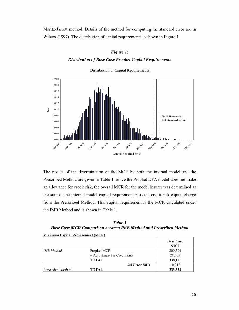
The model was run for the base case assumptions. The Prophet DFA model produced

a distribution of insurance outcomes. For each of these outcomes, the amount of

assets in excess of the technical reserves required at the start of the year to ensure that

the insurer’s assets are equal to their liabilities at the end of the year was determined.

This represents a distribution of capital requirements. The Prophet MCR was

determined as the 99.5th percentile of this distribution of capital requirements. By

taking this capital requirement, the probability that total assets will exceed liabilities

at the end of the year will be 99.5%, using the same simulations. This value was

$309.4M with a standard error of $10.9M. The standard error was calculated using the

20

Maritz-Jarrett method. Details of the method for computing the standard error are in

Wilcox (1997). The distribution of capital requirements is shown in Figure 1.

Figure 1:

Distribution of Base Case Prophet Capital Requirements

Distribution of Capital Requirements

0.000

0.002

0.004

0.006

0.008

0.010

0.012

0.014

0.016

0.018

0.020

-364,9

62

-280,7

40

-196,5

18

-112,2

96

-28,07

4

56,14

8

140,3

70

224,5

92

308,8

14

393,0

36

477,2

58

561,4

80

Capital Required (t=0)

Pro

b.

The results of the determination of the MCR by both the internal model and the

Prescribed Method are given in Table 1. Since the Prophet DFA model does not make

an allowance for credit risk, the overall MCR for the model insurer was determined as

the sum of the internal model capital requirement plus the credit risk capital charge

from the Prescribed Method. This capital requirement is the MCR calculated under

the IMB Method and is shown in Table 1.

Table 1

Base Case MCR Comparison between IMB Method and Prescribed Method

Minimum Capital Requirement (MCR) Base Case $'000 IMB Method Prophet MCR 309,396 + Adjustment for Credit Risk 28,705 TOTAL 338,101 Std Error IMB 10,912 Prescribed Method TOTAL 233,323

99.5th Percentile ± 2 Standard Errors

21

The MCR calculated by the IMB Method was found to be significantly larger than the

MCR under the Prescribed Method. The MCR calculated by the IMB Method

represents the risk-based level of capital required to ensure a ruin probability in one-

year of 0.5%. The Prescribed Method is found to produce a capital requirement

insufficient to ensure a probability of ruin over a one-year time horizon of 0.5%.

To understand each method’s treatment of the various risks we break down each of

the MCRs by line of business and by risk type. The capital charge components that

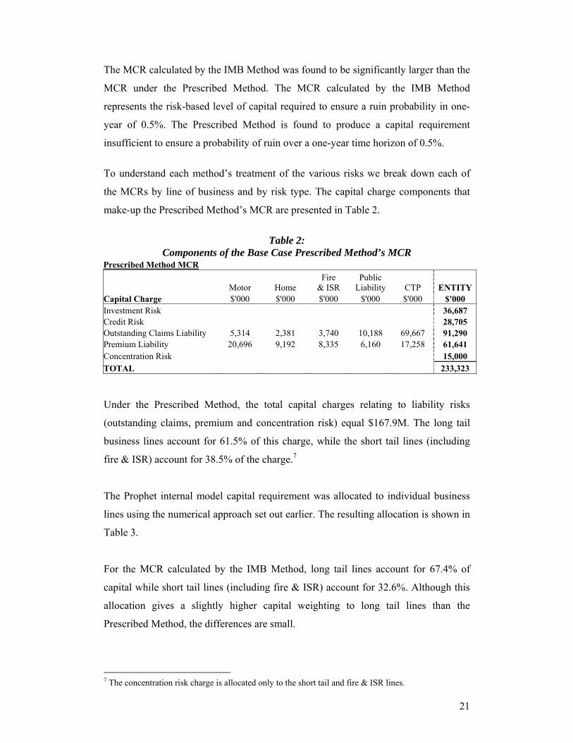
make-up the Prescribed Method’s MCR are presented in Table 2.

Table 2:

Components of the Base Case Prescribed Method’s MCR Prescribed Method MCR

Motor Home Fire

& ISR Public

Liability CTP ENTITYCapital Charge $'000 $'000 $'000 $'000 $'000 $'000 Investment Risk 36,687 Credit Risk 28,705 Outstanding Claims Liability 5,314 2,381 3,740 10,188 69,667 91,290 Premium Liability 20,696 9,192 8,335 6,160 17,258 61,641 Concentration Risk 15,000 TOTAL 233,323 Under the Prescribed Method, the total capital charges relating to liability risks

(outstanding claims, premium and concentration risk) equal $167.9M. The long tail

business lines account for 61.5% of this charge, while the short tail lines (including

fire & ISR) account for 38.5% of the charge.7

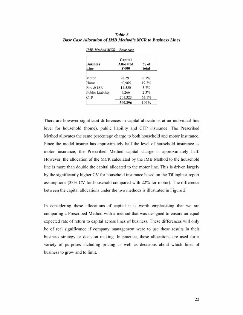
The Prophet internal model capital requirement was allocated to individual business

lines using the numerical approach set out earlier. The resulting allocation is shown in

Table 3.

For the MCR calculated by the IMB Method, long tail lines account for 67.4% of

capital while short tail lines (including fire & ISR) account for 32.6%. Although this

allocation gives a slightly higher capital weighting to long tail lines than the

Prescribed Method, the differences are small.

7 The concentration risk charge is allocated only to the short tail and fire & ISR lines.

22

Table 3

Base Case Allocation of IMB Method’s MCR to Business Lines

IMB Method MCR – Base case

Business Line

Capital Allocated

$'000 % of total

Motor 28,291 9.1% Home 60,965 19.7% Fire & ISR 11,550 3.7% Public Liability 7,266 2.3% CTP 201,323 65.1% 309,396 100%

There are however significant differences in capital allocations at an individual line

level for household (home), public liability and CTP insurance. The Prescribed

Method allocates the same percentage charge to both household and motor insurance.

Since the model insurer has approximately half the level of household insurance as

motor insurance, the Prescribed Method capital charge is approximately half.

However, the allocation of the MCR calculated by the IMB Method to the household

line is more than double the capital allocated to the motor line. This is driven largely

by the significantly higher CV for household insurance based on the Tillinghast report

assumptions (33% CV for household compared with 22% for motor). The difference

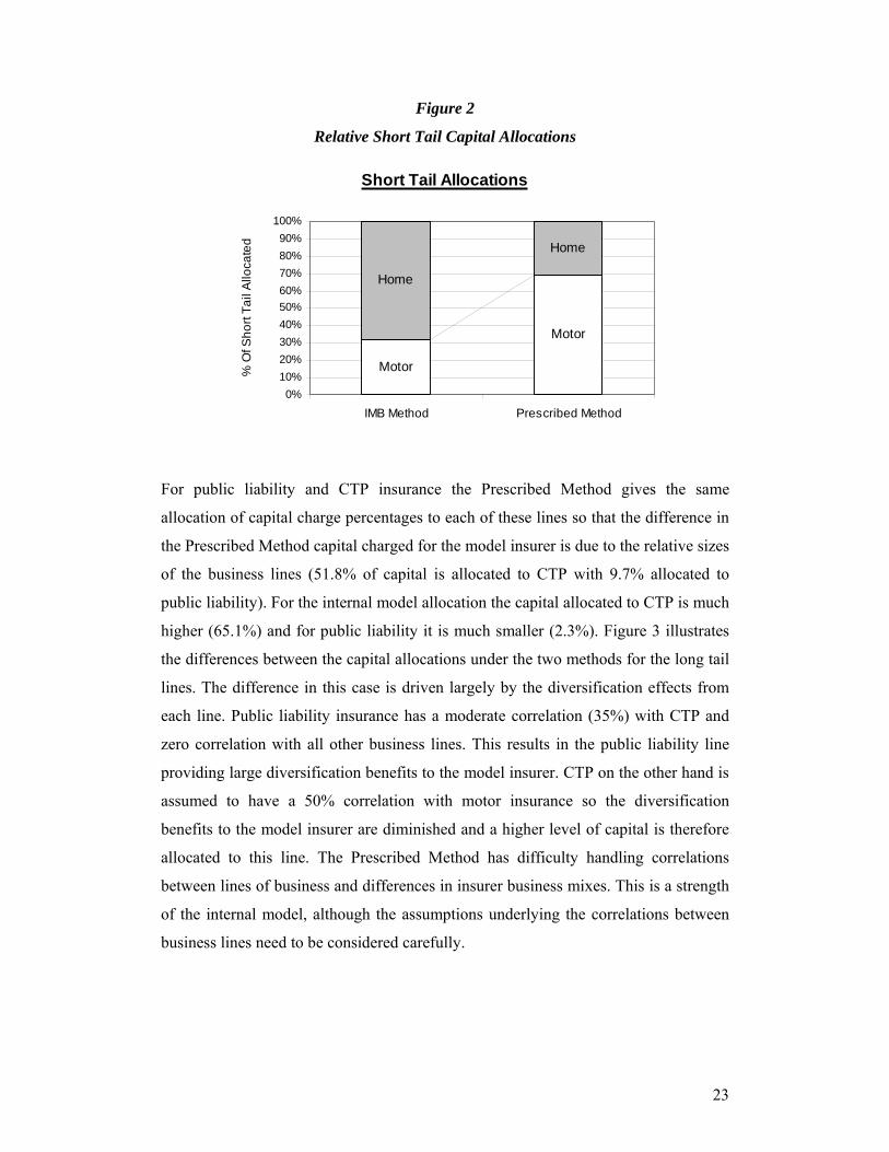
between the capital allocations under the two methods is illustrated in Figure 2.

In considering these allocations of capital it is worth emphasising that we are

comparing a Prescribed Method with a method that was designed to ensure an equal

expected rate of return to capital across lines of business. These differences will only

be of real significance if company management were to use these results in their

business strategy or decision making. In practice, these allocations are used for a

variety of purposes including pricing as well as decisions about which lines of

business to grow and to limit.

23

Figure 2

Relative Short Tail Capital Allocations

Short Tail Allocations

Motor

Motor

Home

Home

0%10%20%30%40%50%60%70%80%90%

100%

IMB Method Prescribed Method

% O

f Sho

rt Ta

il A

lloca

ted

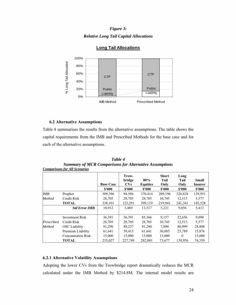
For public liability and CTP insurance the Prescribed Method gives the same

allocation of capital charge percentages to each of these lines so that the difference in

the Prescribed Method capital charged for the model insurer is due to the relative sizes

of the business lines (51.8% of capital is allocated to CTP with 9.7% allocated to

public liability). For the internal model allocation the capital allocated to CTP is much

higher (65.1%) and for public liability it is much smaller (2.3%). Figure 3 illustrates

the differences between the capital allocations under the two methods for the long tail

lines. The difference in this case is driven largely by the diversification effects from

each line. Public liability insurance has a moderate correlation (35%) with CTP and

zero correlation with all other business lines. This results in the public liability line

providing large diversification benefits to the model insurer. CTP on the other hand is

assumed to have a 50% correlation with motor insurance so the diversification

benefits to the model insurer are diminished and a higher level of capital is therefore

allocated to this line. The Prescribed Method has difficulty handling correlations

between lines of business and differences in insurer business mixes. This is a strength

of the internal model, although the assumptions underlying the correlations between

business lines need to be considered carefully.

24

Figure 3:

Relative Long Tail Capital Allocations

Long Tail Allocations

CTPCTP

PublicLiability

PublicLiability

0%

20%

40%

60%

80%

100%

IMB Method Prescribed Method

% L

ong

Tail

Allo

cate

d

6.2 Alternative Assumptions

Table 4 summarises the results from the alternative assumptions. The table shows the

capital requirements from the IMB and Prescribed Methods for the base case and for

each of the alternative assumptions.

Table 4 Summary of MCR Comparisons for Alternative Assumptions

Comparisons for All Scenarios

Base Case

Trow- bridge CVs

80% Equities

Short Tail Only

Long Tail Only

Small Insurer

$'000 $'000 $'000 $'000 $'000 $'000 IMB Prophet 309,396 94,586 370,414 209,196 228,828 139,951 Method Credit Risk 28,705 28,705 28,705 10,745 12,513 5,577 TOTAL 338,101 123,291 399,119 219,941 241,341 145,528 Std Error IMB 10,912 3,469 13,517 5,221 9,056 5,413 Investment Risk 36,391 36,391 85,366 9,157 22,656 9,098 Prescribed Credit Risk 28,705 28,705 28,705 10,745 12,513 5,577 Method OSC Liability 91,290 88,237 91,290 7,890 80,999 28,808 Premium Liability 61,641 59,415 61,641 30,885 23,789 15,876 Concentration Risk 15,000 15,000 15,000 15,000 0 15,000 TOTAL 233,027 227,749 282,001 73,677 139,956 74,359

6.2.1 Alternative Volatility Assumptions

Adopting the lower CVs from the Trowbridge report dramatically reduces the MCR

calculated under the IMB Method by $214.8M. The internal model results are

25

extremely sensitive to the volatility assumptions for the insurance liabilities. An

insurer who uses the Trowbridge CVs for the volatility of their business will require

an MCR under the IMB Method that is significantly lower than the MCR calculated

under the Prescribed Method. Without an extensive study of liability volatility to

validate these assumptions, it is open to insurers who can use the internal model

approach to adopt volatility assumptions in line with these levels.

6.2.2 Riskier Asset Mix

As expected, the MCR under both the IMB and Prescribed Methods increase when the

insurer’s proportion of invested assets in equities is increased to 80%. However, there

is a difference in increase for each method. Under the IMB Method, the MCR

increases by $61.0M while under the Prescribed Method the increase was much less at

only $49.0M. The capital charge for equities in the Prescribed Method may not be

sufficient to allow for the impact of these securities on ruin probabilities.8 Since asset

risk, especially asset mismatch risk, is a major risk run by insurers, a Prescribed

Method should not encourage insurers to adopt a riskier investment strategy. The

above result suggests that the Prescribed Method in Australia may have an incentive

for insurers to invest in equities.

It is interesting to note that had the Trowbridge CV assumptions been used, then

changing the asset mix from 20% equities to 80% equities would have increased the

MCR by a greater amount of $83.7M. The reason for the larger increase under the

Trowbridge assumptions is related to the relative size of the various risks and their

impact on ruin probability. The Trowbridge assumptions have lower insurance

liability volatility, so that fewer of the outcomes at the 99.5th percentile of the capital

required distribution are due to high claims costs. Instead, the outcomes at the 99.5th

percentile are more often due to low asset returns. This leads to a higher proportion of

the overall capital under the IMB Method being attributed to asset risk when insurer

liability volatility assumptions are lower. This in turn creates a greater disparity

between the Prescribed Method’s and IMB Method’s charges for asset risk.

6.2.3 Short Tail Insurer

8 This is based on the assumption that TSM is a realistic model of asset returns.

26

Removing the long tail lines from the insurer reduces the overall insurer’s size along

with the MCR. Under the IMB Method the MCR reduces by $118.2M while under the

Prescribed Method the reduction is significantly larger at $159.3M. The internal

model allocates more capital to each of the insurer’s liabilities than is charged by the

Prescribed Method. So, rather than comparing absolute changes in MCR, it is more

interesting to compare the relative changes. The same will hold for the long tail and

small insurer scenarios.

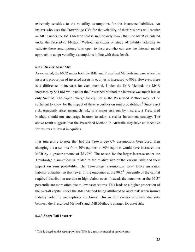
Figure 4 illustrates the MCRs under the different assumptions relative to the base

case.

Figure 4

Alternative Assumptions MCRs as a Percentage of the Base Case

MCR as % of Original

43%

71%65%

60%

32% 32%

0%10%20%30%40%50%60%70%80%90%

100%

Origina

l Sce

nario

Short T

ail O

nly

Long

Tail O

nly

Small In

surer

Scenario

% o

f Orig

inal

IMBPrescribed

For the short tail insurer, the IMB Method has a reduction in its MCR of 65% of its

original size, while under the Prescribed Method the MCR reduces to 32% of its

original size. The internal model is allocating a greater amount of capital to a purely

short tail insurer compared to the Prescribed Method. The reasons for this highlight

some further shortcomings of the Prescribed Method. By reducing the number of lines

of business, diversification benefits are lost. This is accounted for in the IMB Method

but not by the Prescribed Method, which has constant capital charges independent of

the business mix. The result is that the capital calculated under the IMB Method is

higher than under the Prescribed Method.

27

The short tail capital charges (relative to other capital charges) under the Prescribed

Method may also charge less for the risk of those lines than the internal model. This

would be consistent with Collings’ (2001) finding that as an insurer increases its

business mix with short tail lines9, it will have a relatively larger capital increase

under the IMB Method than the Prescribed Method.

This means that insurers will have an incentive to write short tail lines if they are

using the Prescribed Method. If there is a relative advantage in capital required for

short tail lines this may also lead to underpricing of these lines.

6.2.4 Long Tail Insurer

In Figure 4 we note that the MCR calculated by the IMB Method reduces to 71% of

its original size, while under the Prescribed Method the MCR reduces to 60% of its

original size for the case of a long tail insurer. The internal model allocates a higher

level of capital to a purely long tail insurer than the Prescribed Method.

The same two effects as for the short tail insurer appear to apply to the case of the

long tail insurer. Once again there is a loss of some diversification benefits for the

purely long tail insurer leading to the higher relative MCR under the IMB Method

than the Prescribed Method. The long tail capital charges (relative to other capital

charges) under the Prescribed Method charge less for the risk of those lines than the

internal model. This is inconsistent with Collings (2001) findings that increasing the

business mix with long tail lines10 led to a greater relative MCR under the Prescribed

Method than the IMB Method.

However, regardless of the relative impact of long tail lines of business, it is clear that

the Prescribed Method can not deal adequately with differences amongst business mix

of insurers. Applying the Prescribed Methods will lead to incentives for insurers to

change their business mix to optimise their regulatory capital position. Lines of

business with too low capital charges will be increased leading to potential price cuts

that can not be justified if proper risk allowance were to be made.

9 Collings (2001) used motor insurance as an example of a short tail line. 10 Collings (2001) used public liability insurance as an example of a long tail line.

28

6.2.5 Small Insurer

Figure 4 also shows the effect of changing the size of the insurer. In this case the

insurer is assumed to reduce to 25% of its original size. Under the Prescribed Method,

the MCR reduced by a similar amount to 32% of its original size.11 The percentage

capital charges under the Prescribed Method are independent of insurer size. For the

IMB Method, while the size of the insurer decreased, the overall volatility of each of

the business lines is assumed to increase. This is based on the assumption that smaller

business portfolios have greater independent variance and that pooling of insurer risks

reduces relative volatility within a class of business. The volatility assumptions in an

internal model should depend on the size of the business line, with higher volatility

assumed for smaller lines. The overall MCR under the IMB Method reduced to 43%

of its original size.

7. Implications For Risk-based Capital Regulation of

Insurers 7.1 Dependence of Internal Model Results on Volatility Assumptions

These results show the strong dependence of an internal model’s output on the

insurance liability’s volatility assumptions. Of all the sensitivities performed, the

greatest change in MCR resulted from changing from the original Tillinghast

insurance liability CVs to the Trowbridge CVs.

Insurers would be expected to prefer to have a lower regulatory capital requirement.

Insurers in the industry that have liability volatility similar to the Tillinghast CVs are

unlikely to adopt an internal model to calculate their MCR. Insurers that have liability

volatility similar to the Trowbridge CVs have an incentive to adopt an internal model

to lower their MCR. As yet no insurer in Australia has elected to use an internal

model based approach. This may be for a number of reasons. One of these could be

that the Prescribed Method produces lower capital requirements than would be

required if they were to adopt an internal model. If this were the case then those

insurers who use these levels of capital to price their insurance contracts could be

11 The MCR under the Prescribed Method did not reduce to 25% of its original size since the risk margins for a smaller insurer are higher and the concentration charge was assumed to remain constant at $15M.

29

undercharging compared to the premium rate required to generate the level of ruin

probability considered appropriate by APRA using the internal model approach.

The importance of the assumed CVs in determining an insurer’s MCR indicates a

clear need for an assessment of the level of volatility across business lines and an

understanding as to how this varies across companies. Thomson (2003) commented

on APRA’s disappointment with the general lack of justification by actuaries in the

risk margins they adopted for their first reporting under the new APRA requirements.

It appears that the Australian industry is yet to understand fully the true level of

volatility in their insurance business and have yet to reach agreement on best practice

in calculating volatility. This is expected to be an important issue for any regulator to

address, regardless of country, in the introduction of risk-based regulatory capital

requirements.

Issues with the Prescribed Method

Considering the results in Figure 4, it is evident that the Prescribed Method does not

prescribe a level of capital that is adequate to ensure a ruin probability of 0.5% for all

insurers, regardless of size or mix of business. This is based on the presumption that

the internal model used in this study represents an insurer’s realistic business

situation. The model used has been developed to be close to the realistic situation and

reflects industry best practice. The MCR calculated by the internal model should be

representative of the actual level of capital required to ensure a ruin probability in

one-year of 0.5%. Although the IAA Insurer Solvency Assessment Working Party

(2004) state that the Prescribed Method should be conservative to make sure that it is

representative of all insurers that conduct business, in the Australian general insurance

industry this does not appear to be the case.

An important part of implementing the risk-based capital requirements is the

calibration of the Prescribed Method capital charges. APRA calibrated the current

capital charges at an industry-wide level so that the total MCR of the industry

increased by a factor of 1.4 – 1.5 times the previous level. This was a substantial

increase in capital requirements across the industry. The impact of the changes differs

between insurers depending on their experience relative to the industry. Insurers with

lower volatility experience are effectively treated as the same as those with higher

30

volatility experience. Even if the charges are adequate for the average insurer they

may be inadequate for insurers with greater than average volatility. Assuming APRA

want to secure an industry-wide solvency requirement of a 0.5% ruin probability in

one-year then they will need to increase the Prescribed capital charges for insurance

liabilities. Given that the last change in regulatory requirements increased the capital

requirement in the industry by around 50%, a further increase is a politically

contentious issue.

This is the situation that is likely to face many regulators at an international level

when they consider the introduction of these risk-based capital requirements. There

are likely to be poorly capitalised insurers that will no longer be able to operate under

these more stringent requirements. At the same time capital strong insurers will be

expected to meet the requirements. Given the difficult capital situation that has been

faced by the insurance industry at an international level, the adoption of risk-based

capital for insurers may take longer and require more attention to capital weak

insurers than otherwise.

An important issue for the Australian regulator will be to consider the liability capital

charges that should be increased and to what extent. Collings (2001) found that short

tail lines had a relatively higher capital requirement under the IMB Method compared

to the Prescribed Method, and vice versa for long tail lines. While the results from this

study are broadly consistent with this, the differences between long tail and short lines

are less distinct.

At an individual line level, our internal capital allocation showed that the household

line was allocated a significantly larger amount of capital than the motor line. This

was driven by the higher CV assumption for household from the Tillinghast report.

Differences in household and motor volatility suggest that it is inappropriate for

household and motor to have identical capital charges.

Differences in the capital allocations between CTP and public liability were assumed

to be driven largely by diversification effects. Smaller insurers and insurers with less

diversified business mixes are under charged under the Prescribed Method to a greater

extent than larger and well-diversified insurers. This strongly indicates the need to

31

include diversification benefits in the capital requirements, concentration charges for

less diversified insurers or varying capital charges based upon business size.

Further sophistication to the Prescribed Method must be weighed up against the

benefits of simplicity in the method. However it is clear that using a Prescribed

Method that is out of line with the actual risk-based capital requirements will produce

incentives for insurers to behave out of line with the economics of the business. This

is a critical issue if this approach leads to an incentive for insurers to underprice or

grow riskier business lines.

7.3 Investment Risk Capital Charges

Our results demonstrated that the capital required for higher levels of equity

investment was greater under the IMB Method than the Prescribed Method. The

Prescribed capital charge for equities under the model assumptions is insufficient to

cover the risk. This is consistent with the findings of Collings (2001) that the

Prescribed Method is less responsive to increases in equity investment than the IMB

Method. An adequate charge to cover equity risk at the 99.5th percentile would need

to be larger than the current Prescribed charge of 8%,12 particularly for insurers with

investment portfolios that are not well diversified.

On the asset side, the Prescribed Method provides little incentive for insurers with a

well-diversified investment portfolio. As an example to illustrate this point consider

the property investment capital charge. The capital charge for property investment is

10% while the capital charge for listed equity is 8%. For insurers that perceive there

to be relatively higher risk-adjusted returns to be gained from equity than property,

there is an incentive to overweight their investment in equity. This is despite the fact

that there can often be considerable diversification benefits of holding equity and

property together. Collings (2001) provides another example by considering the

diversification and immunisation benefits of holding appropriate amounts of

government bonds and cash. While there is an optimal amount of each of these

securities to hold that minimises overall volatility for the insurer, the capital charges

under the Prescribed Method do not distinguish between the two asset classes and

charge a constant amount of 0.5%.

32

In order to ensure the MCR under the Prescribed Method provides an industry-wide

solvency requirement of a 0.5% ruin probability in one-year, APRA will need to

change the investment capital charges. For risky assets such as equity, the current

capital charges should be increased. APRA should also provide incentives for insurers

to hold well-diversified asset portfolios. This could be achieved by offering

diversification discounts or alternatively a more stringent investment concentration

charge.13

7.4 Incentive to Use an Internal Model

The opening section of APRA’s capital standards states that APRA encourages

insurers with sufficient resources to adopt an internal model for calculation of their

MCR. APRA has a desire for insurers to begin to adopt the IMB Method in line with

its aim for insurers to more closely match their capital requirements with their

individual risk characteristics. The results of the analysis of the capital requirements

that we have undertaken indicate that there is no incentive to adopt the IMB Method

especially if an insurer has insurance liability CVs in line with the Tillinghast report.

The Prescribed Method’s capital charges would need to increase to the extent that the

internal model would produce a lower MCR. Alternatively there needs to be a much

closer examination of the volatility of insurer liabilities and a more careful calibration

of the Prescribed Method capital charges.

There are other reasons why insurers would not adopt an internal model for the MCR

calculation. Even though risk management and measurement techniques in non-life

(property and casualty) insurance have vastly improved over the last decade and DFA

modelling has become an important part of internal management for many large

insurers, developments in these areas are still occurring. The IMB Method requires an

internal model with a very high degree of sophistication to adequately address all the

material risks of an insurer and their complex interrelationships. There also needs to

be the actuarial and risk management human resource skills to ensure proper

implementation and interpretation of results. The internal model used in this study

12 8% is the Prescribed capital charge for listed equity securities. 13 The current investment concentration charge only applies to Grades 4 and 5 debt and does not apply to concentrated holdings in other securities.

33

was based on simplifying assumptions and the internal model for a real-world insurer

would be far more complex. Even with an adequate internal model, the assumptions

required in the model need far more careful attention. A greater understanding and

consensus of the underlying volatility of insurance liabilities is a major requirement

for non-life insurers in order to adopt an internal model for MCR calculation.

Even as actuaries develop the necessary skills and capabilities to adequately

implement an internal model for the IMB Method, there will no doubt exist further

obstacles from other stakeholders in the general insurance industry. The “black-box”

stigma attached to internal models is likely to be an area that actuaries will need to

overcome in order to convince general insurance senior management and the

regulators to trust the internal model’s output for management purposes and MCR

calculation.

Industry experts have identified another obstacle to the IMB Method. Financial

analysts involved in the trading of general insurance company shares may not have

the confidence in the insurer management to rely on them determining their own

regulatory capital requirements. Financial analysts may not be willing to rely upon the

MCR calculated under the IMB Method.

Differences in approaches to internal modelling may also make it difficult to compare

the MCR output from one insurer’s internal model with another insurer. Comparison

across different insurers is important for regulatory reasons and to avoid opportunistic

insurers taking advantage of differences in models. Financial analysts and regulators

may prefer to make MCR comparisons based upon the Prescribed Method where the

formula is fixed and insurer judgement does not impact the results. This leaves open

the need to develop Prescribed Method charges that are more risk-based.

7.5 Further Research

Our results depend to some extent on the degree to which the model and the

assumptions used are representative of actual insurers. Our aim has been to use an

internal model that broadly represents the insurer’s business situation and parameters

and assumptions based on industry best practice. We would expect any insurer that

34

used a model similar to the one that we have used for the IMB approach would come

to similar conclusions.

In this study, many simplifying assumptions were made in the model’s calibration.

We are not aware of any comprehensive study that has been completed that examines

and assesses the appropriate insurance liability volatility assumptions taking into

account actual insurer data and allowing for insurer specific characteristics. This is a

critical area of research required for risk-based regulatory capital if internal models

are to be used with any confidence.

The modelling of claims correlation is another important area for further research.

Dependency models need to be further considered. Brehm (2002) outlines a formal

quantitative approach for estimating correlation from data. The Tillinghast and

Trowbridge reports’ use a much more qualitative approach. Copulas also have great

potential for modelling insurance liability dependencies, especially for tail events.

8. Conclusions The IAA Insurer Solvency Assessment Working Party (2004) has advocated two

methods for non-life insurers to calculate their capital requirement – the Standard

Approach and the Advanced Approach. In Australia, these dual capital requirements

are known as the Prescribed Method and the IMB Method. This study explores the

implications of these new capital requirements.

From APRA’s perspective, the aim is to meet a regulatory objective of requiring that

insurers hold a level of capital to ensure a minimum ruin probability across the

industry. It is important that the Prescribed Method adequately charges risks to meet

this objective for all non-life insurers licensed to do business in Australia.

This study compared the MCRs calculated under the two methods and analysed the

Prescribed Method’s capital charges using a model representative of industry best

practice. Despite this, simplifying assumptions were made in the model’s calibration

and there remains a lack of consensus as to the insurance liability volatility

assumptions.

35

However the results of this study have highlighted some significant issues for both

regulators and insurers. For the model insurer studied, the MCR calculated under the

IMB Method was significantly larger than the MCR under the Prescribed Method.

The implication of this result is that despite APRA’s desire for insurers to adopt an

internal model for MCR calculation, there is an incentive for insurers to use the

Prescribed Method to produce a lower MCR. This also highlights the need to develop

Prescribed Methods that are as consistent with the underlying risk of the insurer. To

do this the need for a diversification allowance is very important.

The results were shown to be highly sensitive to the insurance liability volatility

assumptions. However it is arguable that the current capital charge levels in Australia

are too low in order for the Prescribed Method to ensure a ruin probability in one-year

of less than 0.5% across the entire general insurance industry. This is likely to be very

difficult to achieve. Differences between insurers of different sizes and with different

business mixes should at least be considered more carefully in any revision of the

Prescribed Method capital charges.

There is a strong case for including either diversification benefits or more stringent

concentration charges in the Prescribed Method to address the risk reduction

associated with a well diversified business mix and asset portfolio and to give a more

consistent treatment of insurers with different characteristics.

The internal model’s results rely heavily on its volatility assumptions. There is a

major need for a study to be carried out using insurer level data to develop a

consensus in the industry as to the level of insurance liability volatility that should be

allowed in internal models for capital determination.

We can only conclude that there is much to be done by regulators and insurers if they

are to adopt risk-based capital requirements. Some countries have taken a step along

this path already. Australia has been one of the first countries to introduce a risk-

based regulatory regime for non-life insurers and its experience is no doubt of great

interest to insurers, actuaries and regulators internationally. We have analysed the

capital requirements with a view to identifying lessons for others. There is still a long

36

way to go before insurers will be in a position to confidently adopt the IMB Method

for the MCR calculation even in Australia.

37

References

Australian Prudential Regulation Authority (2002) “General Insurance Prudential Standards and Guidance Notes,” July 2002. www.apra.gov.au Artzner, P., Delbaen, F., Eber, J-M. & Heath, D. (1999) “Coherent Measures of Risk” Mathematical Finance, Vol. 9, 203-228. Basel Committee on Banking Supervision (2001a) “Operational Risk,” January 2001. www.bis.org Basel Committee on Banking Supervision (2001b) “Overview of the New Basel Capital Accord,” January 2001. www.bis.org Basel Committee on Banking Supervision (2001c) “Working Paper on the Regulatory Treatment of Operational Risk,” September 2001. www.bis.org Bateup, R. & Reed, I. (2001) “Research and Data Analysis Relevant to the Development of Standards and Guidelines on Liability Valuation for General Insurance,” Tillinghast Towers-Perrin. Prepared for the Institute of Actuaries of Australia and APRA, November 2001. www.actuaries.asn.au Brehm, P. J (2002) “Correlation and the Aggregation of Unpaid Loss Distributions.” Presented at the Casualty Actuarial Society Fall Forum, 2002. www.casact.org Butsic, R. P (1994) “Solvency Measurement for Property-Liability Risk-Based Capital Applications” The Journal of Risk and Insurance, Vol. 61, 4, 656-690. B&W Deloitte (2003) “How TSM Works – Calibration & Projection.” Prepared for DFA Clients, July 2003. B&W Deloitte (2003) “Prophet DFA User Manual.” Prepared for DFA Clients, January 2003. Casualty Actuaries Society (2002) “Report of the Operational Risks Working Party to GIRO 2002.” www.casact.org Collings, S. (2001) “APRA’s Capital Adequacy Measures: The Prescribed Method v The Internal Model Method.” Presented at the Institute of Actuaries of Australia XIIIth General Insurance Seminar, November 2001.www.actuaries.asn.au Collings, S. & White, G. (2001) “APRA Risk Margin Analysis,” Trowbridge Consulting. Presented at the Institute of Actuaries of Australia XIIIth General Insurance Seminar, November 2001. www.actuaries.asn.au Cummins, J.D. (1988) “Risk-Based Premiums for Insurance Guaranty Funds” The Journal of Finance, Vol. 43, 4, 823-839.

38

Duffie, D. & Pan. J. (1997) “An Overview of Value-at-Risk” The Journal of Derivatives, Spring 1997, 7-49. Dynamic Financial Analysis Committee of the Casualty Actuarial Society (1995) DFA Handbook. Casualty Actuarial Society, September 1995. www.casact.org Embrechts, P., McNeil, A. J. & Straumann, D. (2000) “Correlation: Pitfalls and Alternatives” In Extremes and Integrated Risk Management, ed. Paul Embrechts, Chapter 6, 71-76. London: Risk Books. Financial Services Authority (2003) “Enhanced Capital Requirements and Individual Capital Assessments for Non-Life Insurers,” July 2003. www.fsa.gov.uk Frank, R. H. & Bernanke B.S. (2001) “The Economics of Information” Principles of Microeconomics, McGraw Hill Irwin, First Edition 2001, 297-312. Giese, G. (2003) “Economic Capital versus Regulatory Capital – A Market Benchmark,” Risk, May 2003. www.risk.net Gray, B. (2001) “Prudential Supervision of General Insurance – Policy Discussion Paper,” APRA, March 2001. www.apra.gov.au Gray, B. (1999) “Study of the Prudential Supervisory Requirements for General Insurers in Australia,” APRA, September 1999. www.apra.gov.au Holton, G. (2003) Value-at-Risk: Theory and Practice, Academic Press, March 2003. IAA Insurance Regulation Committee (2002) “Report of Solvency Working Party,” February 2002. This can be found at www.actuaries.org IAA Insurer Solvency Assessment Working Party (2003) “A Global Framework for Insurer Solvency Assessment,” May 2003. www.actuaries.org IAA Insurer Solvency Assessment Working Party (2004) “A Global Framework for Insurer Solvency Assessment: Appendix B – Non-life Case Study,” www.actuaries.org Klugman, S. A., Panjer, H. H. & Willmot, G. E. (1998) “Aggregate Loss Models” In Loss Models: From Data to Decisions, Chapter 4, 291-384. USA: John Wiley & Sons. Mack, T. (1993) “Distribution Free Calculation of the Standard Error of Chain Ladder Reserve Estimates” ASTIN Bulletin, Vol. 23, 2, 213-225. Myers, S. C. & Read Jr., J. A. (2001) “Capital Allocation for Insurance Companies” Journal of Risk and Insurance, Vol. 68, 4, 545-580 Rockafellar, R. T. & Uryasev, S. (2002) “Conditional Value-at-Risk for General Loss Distributions” Journal of Banking and Finance, Vol. 26, 1443-1471.

39

Sherris, M. (2003) “Equilibrium Insurance Pricing, Market Value of Liabilities and Optimal Capitalization,” University of NSW. Presented at the 13th International AFIR Colloquium, Maastricht, Netherlands, September 2003. www.actuarial.unsw.edu.au Sherris, M., “Solvency, Capital Allocation and Fair Rate of Return in Insurance”, UNSW Actuarial Studies Working Paper (2004) http://www.actuary.unsw.edu.au/files/sherriscapall.pdf Slater, D. & Gillott, N. (2003) “Calibration of the General Insurance Risk Based Capital Model,” Watson Wyatt UK. Prepared for the Financial Services Authority, July 2003. www.fsa.gov.uk Stevens, A. & Tadros, R. (2003) “Getting the Solvency Balance Right” Risk, May 2003. www.risk.net Sutherland-Wong, C., (2003), “A Comparison of Methods for APRA’s General Insurance Capital Requirements”, BCom Honours Thesis, Actuarial Studies, University of News South Wales. Taylor, G. (1995) “An Equilibrium Model of Insurance Pricing and Capitalization” Journal of Risk and Insurance, Vol. 62, 3, 408-446 Taylor, G. (2000) “Stochastic Models” In Loss Reserving: An Actuarial Perspective, Part II, 167-228. US: Kluwer. Thomson, R. (2003) “The Approved Actuary Regime in General Insurance – An APRA Reflection” Actuary Australia, July 2003, 12-13. www.actuaries.asn.au Venter, G. (2001) “Tails of Copulas.” Presented at the ASTIN Colloquium, Washington, USA, July 2001. www.actuaries.org Wilcox, R. R. (1997) “Estimating Measures of Location and Scale” In Introduction to Robust Estimation and Hypothesis Testing, Chapter 3, p41. USA: Academic Press Information on The Smith Model (TSM) can be found at www.thesmithmodel.com

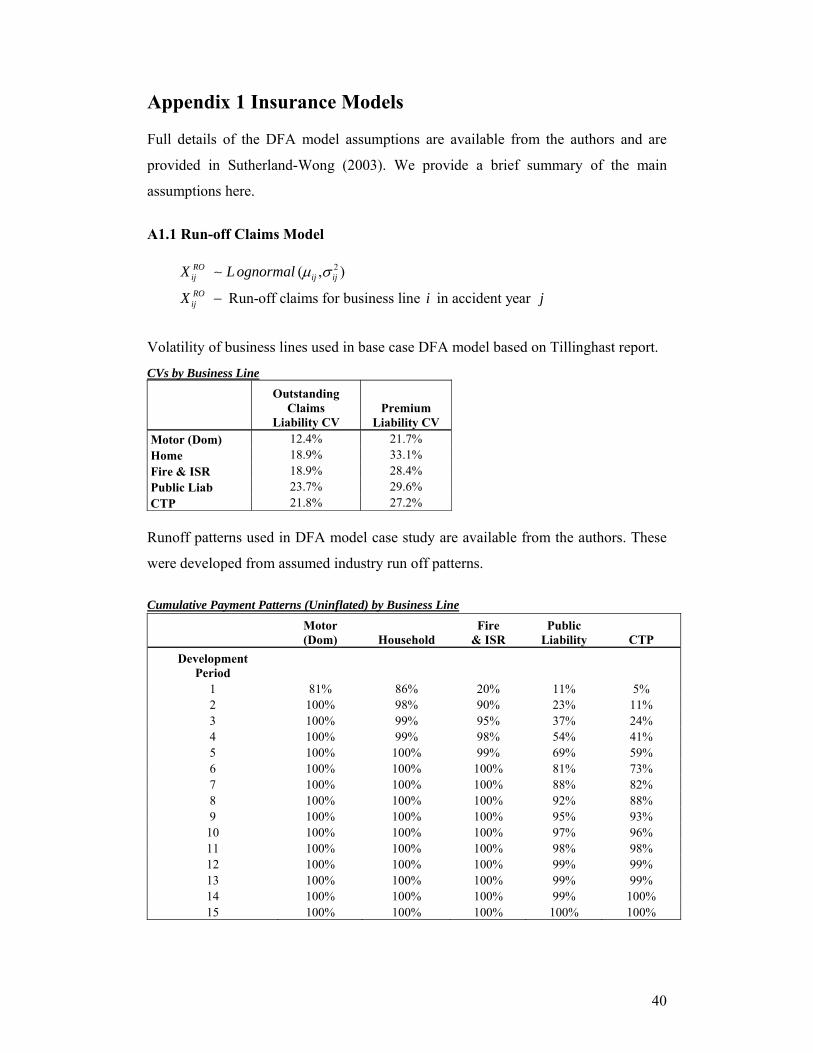
40

Appendix 1 Insurance Models Full details of the DFA model assumptions are available from the authors and are

provided in Sutherland-Wong (2003). We provide a brief summary of the main

assumptions here.

A1.1 Run-off Claims Model

2( , )

Run-off claims for business line in accident year

ROij ij ij

ROij

X L ognormal

X i j

µ σ

−

∼

Volatility of business lines used in base case DFA model based on Tillinghast report.

CVs by Business Line

Outstanding Claims

Liability CV Premium

Liability CV Motor (Dom) 12.4% 21.7% Home 18.9% 33.1% Fire & ISR 18.9% 28.4% Public Liab 23.7% 29.6% CTP 21.8% 27.2% Runoff patterns used in DFA model case study are available from the authors. These

were developed from assumed industry run off patterns.

Cumulative Payment Patterns (Uninflated) by Business Line

Motor (Dom) Household

Fire & ISR

Public Liability CTP

Development Period

1 81% 86% 20% 11% 5% 2 100% 98% 90% 23% 11% 3 100% 99% 95% 37% 24% 4 100% 99% 98% 54% 41% 5 100% 100% 99% 69% 59% 6 100% 100% 100% 81% 73% 7 100% 100% 100% 88% 82% 8 100% 100% 100% 92% 88% 9 100% 100% 100% 95% 93% 10 100% 100% 100% 97% 96% 11 100% 100% 100% 98% 98% 12 100% 100% 100% 99% 99% 13 100% 100% 100% 99% 99% 14 100% 100% 100% 99% 100% 15 100% 100% 100% 100% 100%

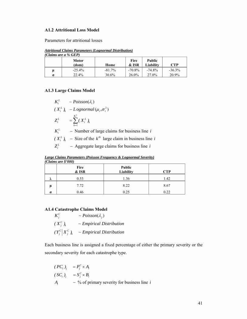
41

A1.2 Attritional Loss Model Parameters for attritional losses Attritional Claims Parameters (Lognormal Distribution) (Claims are a % GEP)

Motor (dom) Home

Fire & ISR

Public Liability CTP

µ -25.4% -81.7% -70.8% -74.8% -36.3% σ 22.4% 30.6% 26.0% 27.0% 20.9%

A1.3 Large Claims Model

2

1

( )

( , )

Number of large claims for business line

Size of the large claim in business line

Aggregate large claims for business

Li

Li i

Li k i i

KL Li i k

kLi

L thi k

Li

K Poisson

( X ) L ognormal

Z ( X )

K i

( X ) k i

Z

λ

µ σ

=

=

−

−

−

∑

∼∼

line i

Large Claims Parameters (Poisson Frequency & Lognormal Severity) (Claims are $’000)

Fire

& ISR Public

Liability CTP

λ 0.53 1.36 1.42

µ 7.72 8.22 8.67

σ 0.46 0.25 0.22

A1.4 Catastrophe Claims Model

( )Cj j

Cj k

C Cj j k

K Poisson

( X ) Empirical Distribution

(Y X ) Empirical Distribution

λ∼

∼

∼

Each business line is assigned a fixed percentage of either the primary severity or the

secondary severity for each catastrophe type.

% of primary severity for business line

Ci j j i

Ci j j i

i

( PC ) P A

( SC ) S B

A i

= ×

= ×

−

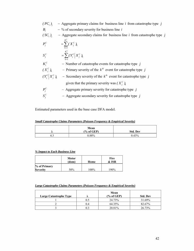
42

Aggregate primary claims for business line from catastrophe type

% of secondary severity for business line Aggregate secondary claims for business line from catastrophe typ

i j

i

i j

( PC ) i j

B i( SC ) i

−

−− e j

1

1

Number of catastrophe events for catastrophe type

Primary severity of the event for catastrophe type

Secondary severity of the

Cj

Cj

KC Cj j k

k

KC C Cj j j k

k

Ci

C thj k

C C tj j k

P ( X )

S (Y X )

K j

( X ) k j

(Y X ) k

=

=

=

=

−

−

−

∑

∑

event for catastrophe type

given that the primary severity was

Aggregate primary severity for catastrophe type

Aggregate secondary severity for catastrophe type

h

Cj k

Cj

Cj

j

( X )

P j

S j

−

−

Estimated parameters used in the base case DFA model. Small Catastrophe Claims Parameters (Poisson Frequency & Empirical Severity)

λ Mean

(% of GEP) Std. Dev 4.3 0.88% 0.43%

% Impact to Each Business Line

Motor (dom) Home

Fire & ISR

% of Primary Severity 50% 100% 190% Large Catastrophe Claims Parameters (Poisson Frequency & Empirical Severity)

Large Catastrophe Type λ Mean

(% of GEP) Std. Dev 1 0.5 24.73% 31.69% 2 0.4 64.35% 82.67% 3 0.3 20.81% 26.73%

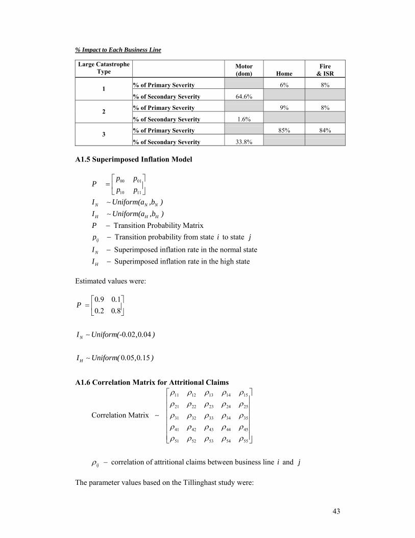
43

% Impact to Each Business Line

Large Catastrophe Type

Motor (dom) Home

Fire & ISR

% of Primary Severity 6% 8% 1 % of Secondary Severity 64.6%

% of Primary Severity 9% 8% 2 % of Secondary Severity 1.6%

% of Primary Severity 85% 84% 3 % of Secondary Severity 33.8%

A1.5 Superimposed Inflation Model

00 01

10 11

Transition Probability Matrix Transition probability from state to state

Superimposed inflation rate in the normal state Superimp

N N N

H H H

ij

N

H

p pP

p pI Uniform(a ,b )I Uniform(a ,b )Pp i j

II

⎡ ⎤= ⎢ ⎥⎣ ⎦

−−

−−

∼∼

osed inflation rate in the high state

Estimated values were:

0 9 0 10 2 0 8

0 02 0 04

0 05 0 15

N

H

. .P

. .

I Uniform(- . , . )

I Uniform( . , . )

⎡ ⎤= ⎢ ⎥⎣ ⎦

∼

∼

A1.6 Correlation Matrix for Attritional Claims 11 12 13 14 15

21 22 23 24 25

31 32 33 34 35

41 42 43 44 45

51 52 53 54 55

Correlation Matrix

correlation of attritional claims between business line and ij i j

ρ ρ ρ ρ ρρ ρ ρ ρ ρρ ρ ρ ρ ρρ ρ ρ ρ ρρ ρ ρ ρ ρ

ρ

⎡ ⎤⎢ ⎥⎢ ⎥⎢ ⎥⎢ ⎥⎢ ⎥⎢ ⎥⎣ ⎦

−

∼

The parameter values based on the Tillinghast study were:

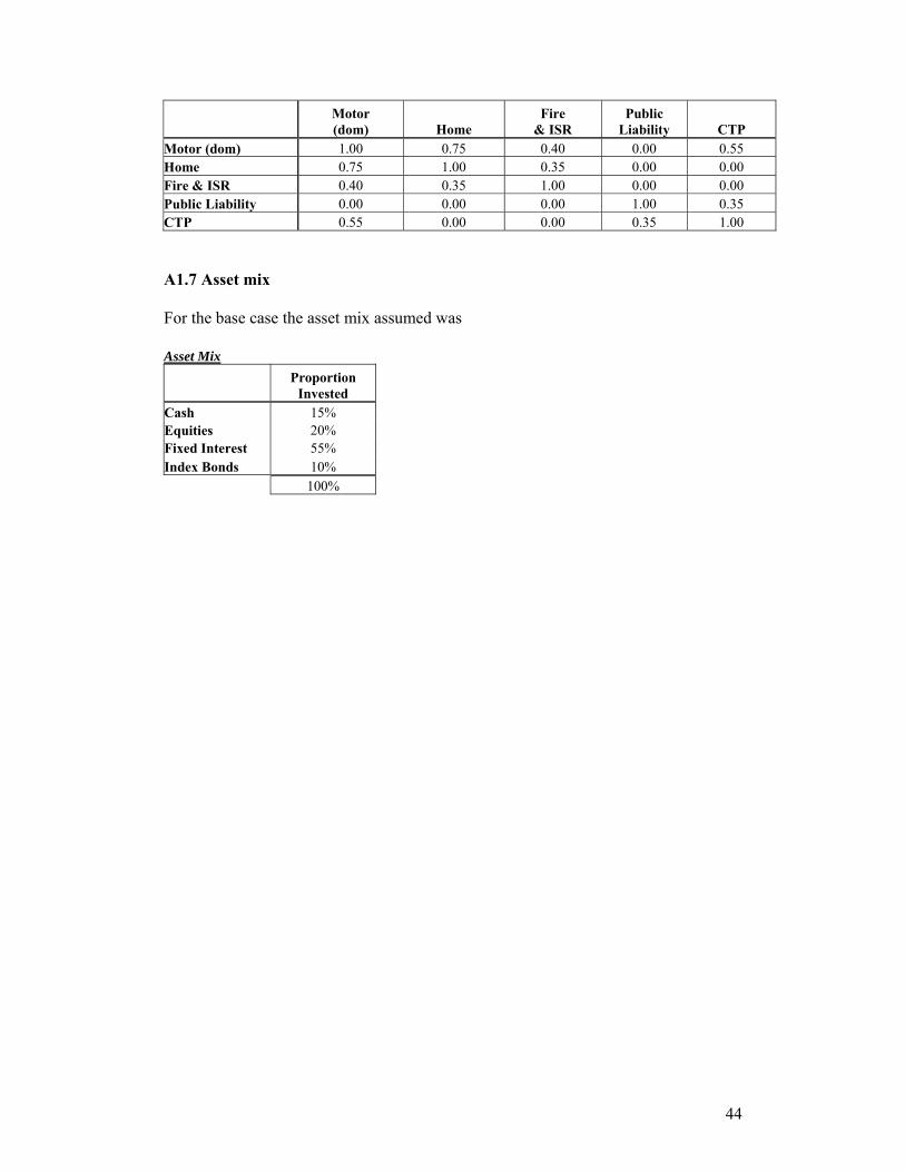
44

Motor (dom) Home

Fire & ISR

Public Liability CTP

Motor (dom) 1.00 0.75 0.40 0.00 0.55 Home 0.75 1.00 0.35 0.00 0.00 Fire & ISR 0.40 0.35 1.00 0.00 0.00 Public Liability 0.00 0.00 0.00 1.00 0.35 CTP 0.55 0.00 0.00 0.35 1.00 A1.7 Asset mix For the base case the asset mix assumed was Asset Mix

Proportion

Invested Cash 15% Equities 20% Fixed Interest 55% Index Bonds 10% 100%

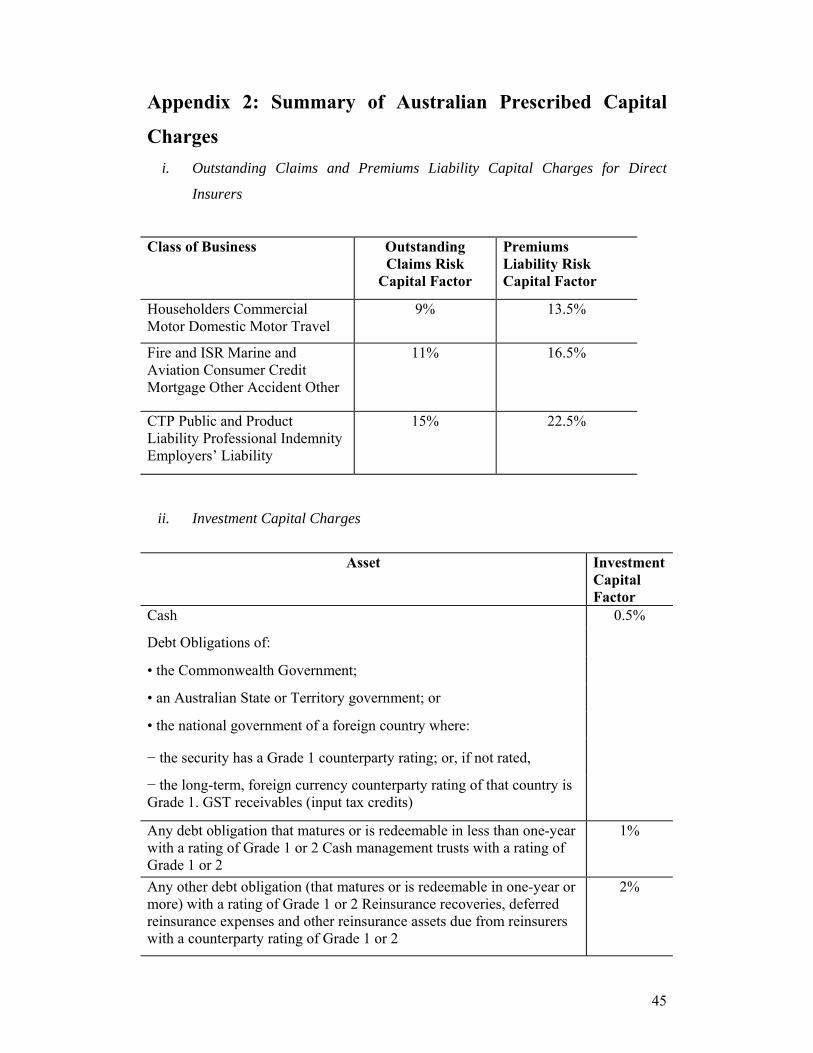
45

Appendix 2: Summary of Australian Prescribed Capital

Charges i. Outstanding Claims and Premiums Liability Capital Charges for Direct

Insurers

Class of Business Outstanding Claims Risk

Capital Factor

Premiums Liability Risk Capital Factor

Householders Commercial Motor Domestic Motor Travel

9% 13.5%

Fire and ISR Marine and Aviation Consumer Credit Mortgage Other Accident Other

11% 16.5%

CTP Public and Product Liability Professional Indemnity Employers’ Liability

15% 22.5%

ii. Investment Capital Charges

Asset Investment

Capital Factor

Cash 0.5%

Debt Obligations of:

• the Commonwealth Government;

• an Australian State or Territory government; or

• the national government of a foreign country where:

− the security has a Grade 1 counterparty rating; or, if not rated,

− the long-term, foreign currency counterparty rating of that country is Grade 1. GST receivables (input tax credits)

Any debt obligation that matures or is redeemable in less than one-year with a rating of Grade 1 or 2 Cash management trusts with a rating of Grade 1 or 2

1%

Any other debt obligation (that matures or is redeemable in one-year or more) with a rating of Grade 1 or 2 Reinsurance recoveries, deferred reinsurance expenses and other reinsurance assets due from reinsurers with a counterparty rating of Grade 1 or 2

2%

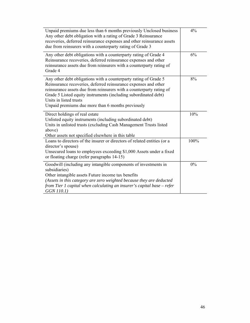
46

Unpaid premiums due less than 6 months previously Unclosed business Any other debt obligation with a rating of Grade 3 Reinsurance recoveries, deferred reinsurance expenses and other reinsurance assets due from reinsurers with a counterparty rating of Grade 3

4%

Any other debt obligations with a counterparty rating of Grade 4 Reinsurance recoveries, deferred reinsurance expenses and other reinsurance assets due from reinsurers with a counterparty rating of Grade 4

6%

Any other debt obligations with a counterparty rating of Grade 5 Reinsurance recoveries, deferred reinsurance expenses and other reinsurance assets due from reinsurers with a counterparty rating of Grade 5 Listed equity instruments (including subordinated debt) Units in listed trusts Unpaid premiums due more than 6 months previously

8%

Direct holdings of real estate Unlisted equity instruments (including subordinated debt) Units in unlisted trusts (excluding Cash Management Trusts listed above) Other assets not specified elsewhere in this table

10%

Loans to directors of the insurer or directors of related entities (or a director’s spouse) Unsecured loans to employees exceeding $1,000 Assets under a fixed or floating charge (refer paragraphs 14-15)

100%

Goodwill (including any intangible components of investments in subsidiaries) Other intangible assets Future income tax benefits (Assets in this category are zero weighted because they are deducted from Tier 1 capital when calculating an insurer’s capital base – refer GGN 110.1)

0%