1

Risk contributions in an asymptotic multi­factor framework

Dirk Tasche∗†

May 20, 2005

Abstract

So far, regulatory capital requirements for credit risk portfolios are calculated in a bottom­up approach by determining the requirements at asset level and then adding up them. In

contrast, economic capital for a credit risk portfolio is calculated for the portfolio as a whole

and then decomposed into risk contributions of assets or sub­portfolios for, e.g., diagnostic

purposes like identifying risk concentrations. In the “Asymptotic Single Risk Factor” model that underlies the most important part of the “Basel II Accord”, bottom­up and top­down

approach yield identical results. However, the model fails in detecting exposure concentra­tions and recognizing diversification effects. We investigate multi­factor extensions of the

ASRF model and derive exact formulae for the risk contributions to Value­at­Risk and Ex­pected Shortfall. As an application of the risk contribution formulae we introduce a new

concept for a diversification index. The use of this new index is illustrated with an example

calculated with a two­factor model. The results with this model indicate that there can be

a substantial reduction of risk contributions by diversification effects.

Introduction

Credit risk, i.e. the risk that borrowers do not fully meet their obligations, is considered the most important risk banks are facing. During the past decade, therefore, banks as well as banking

supervisory authorities put considerable efforts in developing models for quantitative assessments of credit risk. These efforts were accompanied by a growing interest of the academic community

in credit risk models. Compared to models of market risk or actuarial models, credit risk models have some interesting special features. In particular, they produce non­normal loss distributions and reflect the empirically observed dependence of credit events.

While the more advanced large banks rely more and more on very sophisticated credit risk

models in order to take into account these features, banking supervisors worldwide intend to ∗Deutsche Bundesbank, Postfach 10 06 02, 60006 Frankfurt am Main, Germany

E­mail: tasche@ma.tum.de †The opinions expressed in this paper are those of the author and do not necessarily reflect views of Deutsche

Bundesbank. The author thanks Katja Pluto for useful comments on an earlier version of the paper.

1

implement a minimum standard of credit risk modelling which can also be met by smaller banks. The process of designing this standard (“Basel II”) is coordinated by the Basel Committee

on Banking Supervision (BCBS). Although some details are still under discussion, the BCBS

published at the end of June 2004 a framework with the status quo of its recommendations (BCBS, 2004). Most important in this so­called “Basel II Accord” is the part on the “Internal Ratings Based Approach” (IRBA) for the determination of regulatory capital requirements for credit risk. It is regarded as a first step towards a supervisory recognition of advanced credit risk models and economic capital calculations.

According to the IRBA, the regulatory minimum capital for a credit risk portfolio is calculated

in a bottom­up approach by determining capital requirements at asset level and adding up them. The capital requirements of the assets are expressed as 8 percent of the so­called “risk weights”. The risk weight functions were developed by considering a special credit portfolio model, the

so­called “Asymptotic Single Risk Factor Model” (ASRF model, Gordy, 2003). This model is characterized by its computational simplicity and the property that the risk weights of single

credit assets depend only upon the characteristics of these assets, but not upon the composition

of the portfolio (“portfolio invariance”). As a consequence, the model can reflect neither exposure

concentrations nor segmentation effects (say by industry branches).

The model’s inability to detect exposure concentrations entails a potential underestimation

of the risk inherent in the portfolio, whereas its fault in recognizing the diversification effects following from segmentation could result in a potential overestimation of portfolio risk. The Basel Committee decided to deal in Pillar 2 of the Basel II Accord (BCBS, 2004) with the potential underestimation of risk concentration. As a consequence there is no automatism of extended

regulatory capital requirements for risk concentrations, but banks will have to demonstrate

to the supervisors that they have established appropriate procedures to keep concentrations under control. Nevertheless, there are methods to measure quantitatively risk concentrations. A quantitative way of tackling the exposure concentration issue was suggested in Emmer and

Tasche (2005), for instance.

In the present paper, we suggest a minimal – in the spirit of Emmer and Tasche (2005) –

extension of the Basel II model that allows to study the effects of segmentation on portfolio risk. Admitting several risk factors instead of a single factor only and applying the same transition

to the limit as described in Gordy (2003), we arrive at versions of the model that remove the

no segmentation restriction. Alternatively, our class of models can be regarded as special cases of the asymptotic models introduced by Lucas et al. (2001, Theorem 1).

As determining risk contributions or, economically speaking, capital requirements for assets or sub­portfolios, is a main purpose when using credit risk models, deriving exact formulae for risk

contributions to “Value­at­risk” (VaR) and “Expected Shortfall” (ES) in the asymptotic multi risk factors setting represents the main contribution of our paper to the subject. Our results complement results on the differentiation of VaR and ES presented in Gourieroux et al. (2000),

2

�

2

Lemus (1999), and Tasche (1999). From a computational point of view, the resulting formulae

are more demanding than in the one factor case, and – necessarily, as otherwise diversification

effects could not be recognized – they are not portfolio invariant any longer. As an application

of the risk contribution formulae we introduce then a new concept for a diversification index. This index can be computed at portfolio as well as at sub­portfolio or asset level, thus allowing

for identifying the causes of bad diversification. The use of these new indices is illustrated with

an example calculated with a two­factor model. The results with this model indicate that there

can be a substantial reduction of risk contributions by diversification effects.

The material presented here is closely related to work by Pykhtin (2004) and Garcia et al. (2004). Pykhtin describes an approximation of multi­factor models by single­factor models, thus transferring the computational simplicity of single­factor models to multi­factor models. Garcia

et al. propose “factor adjustments” to the risk contributions from a single­factor model in order to

reflect diversification effects. As our results on the risk contribution formulae are not approximate

but exact they could be used for benchmarking the results by Pykhtin and Garcia et al.

This paper is organized as follows: In Section 2 we introduce the class of models we are going

to analyze and derive some basic properties. In Section 3 we shortly recall the Euler allocation

principle that justifies the use of partial derivatives as risk contributions and derive then the

announced formulae for risk contributions to VaR and ES in the asymptotic multi­factor setting. A potential application of the risk contribution formulae for the purpose of identifying sources of concentration risk is suggested in Section 4 where a new concept for a diversification index

is introduced. Section 5 gives a numerical illustration of a potential application of the formulae

and the diversification index. We conclude with some summarizing comments in Section 6.

Asymptotic multi­factor models: basic properties

The starting point for the factor models1 we are going to consider is a random variable L(u) =

L(u1, . . . , un) that reflects the loss suffered from a portfolio of n credit assets, with respective

exposures ui. The tilde indicates that we regard the original loss variable, without any approxi­mation procedure. The variable L(u) can be interpreted as the absolute loss, measured in units of some currency. Then the ui are absolute exposures2 and amounts of money. Alternatively, L(u) can also be understood as relative loss, indicating the percentage of the sum of all exposures that is lost. In this case the ui are non­negative numbers without units that add up to 1.

Formally, the original loss variable L(u) is given as n

L = ui 1Di . (2.1) i=1

1See Bluhm et al. (2002) and the references therein for more information on credit risk models. 2 ui may be thought as a face value multiplied with some factor that expresses the average loss rate in case of

default.

3

�

�� �

The term 1Di is the default indicator variable for asset i, i.e. it takes the value of 1 if i defaults and 0 if not. As a consequence, the sum in (2.1) will be built up with only those ui’s that relate

to defaulted assets i. For factor models, it is quite common to specify the default events Di by ��k � Di = ρi,j Sj + ωi ξi ≤ ti , i = 1, . . . , n, (2.2)

j=1

with the following for the involved constants and random variables:

• The random variables S1, . . . , Sk are the systematic risk factors. They are assumed to

capture the dependence of the default events. In general, we have k � n. Within this paper, we assume that the factor variables are standardized, i.e.

E[Sj ] = 0 and var[Sj ] = 1, j = 1, . . . , k. (2.3)

The S1, . . . , Sk may be stochastically dependent, but they do not have do be.

• The random variables ξ1, . . . , ξn are the idiosyncratic risk drivers. They are also standard­ized, i.e.

E[ξi] = 0 and var[ξi] = 1, i = 1, . . . , n. (2.4)

ξ1, . . . , ξn, (S1, . . . , Sk ) are stochastically independent. As a consequence, conditional on

(S1, . . . , Sk ), the default events Di, i = 1, . . . , n are independent.

• The constants ρi,j , i = 1, . . . , n, j = 1, . . . , k are the factor loadings of the systematic

factors. We assume that k

ρi,j ρi,� corr[Sj , S�] ≤ 1, i = 1, . . . , n. (2.5) j=1,�=1

By (2.5) and the standardization assumption on the Sj and ξi the idiosyncratic loadings

ωi, i = . . . , n are well defined by � k

ωi = �1 − ρi,j ρi,� corr[Sj , S�]. (2.6) j=1,�=1

As a further consequence of (2.5) and (2.6) and of the standardization assumptions also

the asset values changes �k

j=1 ρi,j Sj + ωi ξi are standardized.

• The constant ti, i = 1, . . . , n is called default threshold. It can be thought as a critical loss in value of borrower i’s assets that causes the borrower to default on asset i. It is common

to derive ti from borrower i’s (assumed to be known) probability of default pi. Hence, we

determine ti such that � �k � P[Di] = P ρi,j Sj + ωi ξi ≤ ti = pi, i = 1, . . . n. (2.7)

j=1

When the idiosyncratic risk drivers ξi and the factor variables are all standard normally

distributed, also the asset value changes �

jk =1 ρi,j Sj + ωi ξi are standard normal. Let Φ

denote the standard normal distribution function. By (2.7) we then have pi = Φ(ti).

4

��

�

�

� � � ��� � � � � � ��

� � � �

�

� � �

� � � �

For the sake of a more concise notation we define

S = (S2, . . . , Sk), s� = (s2, . . . , sk) (2.11a)

and for fixed u n

G(v, s�) = uj gj(v, s�). (2.11b) j=1

By Assumption 2.2, then, for fixed s�, v �→ G(v, s�) is invertible. Write G(·, s�)−1 for the inverse

function of v �→ G(v, s�). Write additionally G(·, s�)−1(0) = ∞ and G(·, s�)−1(z) = −∞ for z ≥ n j=1 uj . Having fixed the assumptions and notations, we can prove a result on the calculation

of moments that in particular implies that the distribution of the generalized loss variable L(u) has a density.

Proposition 2.3 Let F : [0, 1] → R be arbitrary and L(u) be the loss variable defined by (2.10). nThen, under Assumption4 2.2, for any 0 ≤ z ≤ j=1 uj and i ∈ {1, . . . , n} we have: � � � � � �� � � z F gi(G(·, S)−1(t), S) h G(·, S)−1(t) | S

E F (gi(S)) 1{L(u)≤z} = − 0

E ∂ G(v, S)��

v=G(·,S)−1 (t)

dt. ∂v �

Proof.

E F (gi(S)) 1{L(u)≤z} = E F (gi(S1, S)) 1 {G(S1,S)≤z} | S = s� PS�−1(ds�) (2.12a)

(taking into account G(·, s�)−1(0) = ∞)

= ∞

F gi(y, s�) h(y | s�) dy PS�−1(ds�) (2.12b) s)−1(z)G(·,�

(substituting y = G(·, s�)−1(t)) � � � � � � z F gi(G(·, s�)−1(t), s�) h G(·, s�)−1(t) | s�

= − 0

∂ G(v, S)�� v=G(·,S)−1(t)

dtPS�−1(ds�). ∂v �

The assertion follows by applying Fubini’s theorem. 2

The choice F = 1 in Proposition 2.3 implies the existence of a density for the distribution of the

generalized loss variable:

Corollary 2.4 Under Assumption 2.2, the loss variable L(u) from (2.10) has the density fL(u) : n0, j=1 uj → [0,∞[, defined by ⎡ ⎤

fL(u)(t) = −E h G(·, S)−1(t) | S � �n � ⎣

∂ G(v, S)�� v=G(·,S)−1 (t)

⎦ , t ∈ 0, uj . (2.13)� j=1 ∂v �

4In order to keep the representation of the results as intuitive and clear as possible here and in the following the

proofs will not be rigorous but rather consist of calculations without consideration of continuity, differentiability

etc. Moreover, for some of the results, additional assumptions on existence of moments etc. must be made.

6

� � � � | �

�

Note that Gordy’s (2003) ASRF (Asymptotic Single Risk Factor) model is a special case of (2.8) with k = 1. Then the expectation in (2.13) disappears, and the density h and the inverse of G

do not depend on s�. Nevertheless, in the case of non­constant asset correlations or probabilities of default the calculation of the density of L(u) will involve numerical inversion of G even in the

simple ASRF case.

In case that an explicit representation of the conditional distribution of S1 given S� is known

(e.g. if S is jointly normally distributed), Equation (2.12a) (with F = 1) yields a more efficient way to calculate the distribution function of L(u) than Corollary 2.4 does. The reason is that application of Corollary 2.4 would require evaluation of a k­dimensional integral if S had a

density, whereas the application of the following Proposition 2.5 would only require evaluation

of a (k − 1)­dimensional integral.

Proposition 2.5 Under Assumption 2.2, the distribution function of the loss variable L(u) as

given in (2.10) can be calculated by means of

P[L(u) ≤ z] = P S1 ≥ G(·, S)−1(z) S = s� PS�−1(ds�). (2.14)

Define, for α ∈ (0, 1) and any real random variable X , the α­quantile of X by

qα(X ) = min{x : P[X ≤ x] ≥ α}. (2.15a)

Quantiles at high levels (e.g. 99.9%) are popular metrics for determining the economic capital of portfolios. Within the financial community, the α­quantile of a loss distribution is commonly

called Value­at­Risk (VaR) at level α. In case of the generalized loss variable L(u) we write

qα(L(u)) = qα(u). (2.15b)

The quantiles of L(u) can be computed by numerical inversion of (2.14).

We conclude this section by providing two alternative formulae for the calculation of another popular risk measure, the Expected Shortfall5, in the case of the asymptotic multi­factor model under consideration.

Remark 2.6 The Expected Shortfall ESα(L(u)) = E[L(u) L(u) ≥ qα(L(u))] at level α of the |loss variable L(u) from (2.10) can alternatively be calculated with recourse to Corollary 2.4 or

to Proposition 2.5. Note that the existence of a density of the distribution of L(u) (Corollary

2.4) implies P[L(u) ≥ qα(L(u))] = 1 − α. From Corollary 2.4 we can therefore derive ⎡ ⎤ � �n � � j=1 uj � �

E[L(u) L(u) ≥ qα(L(u))] = −(1 − α)−1 t E h G(·, S�)−1(t) | S ⎦ dt. (2.16a)|

qα(L(u))

⎣ ∂ G(v, S)�

v=G(·,S)−1(t)∂v �See Acerbi and Tasche (2002) and the references given there for more details on Expected Shortfall vs. Value­

at­Risk. In particular, in case of discontinuous loss distributions the definition of ES has to be slightly modified

in order to make it a risk measure superior to VaR.

7

5

�

| � � � � � �

�

� � � �

∞0 P[X ≥ x] dx forFrom Proposition 2.5 we obtain (by making use of the formula E[X] =

X ≥ 0)

E[L(u) L(u) ≥ qα(L(u))] (2.16b) n j=1 uj

S)−1(z)

qα (L(u))

�

3 Computing the risk contributions

When economic capital for a portfolio is determined by means of a homogeneous risk measure, by the Euler allocation principle the risk contributions of assets should be calculated as partial derivatives of the portfolio­wide economic capital with respect to the exposures. In this section

we first recall the Euler principle and derive then formulae for the derivatives of Value­at­Risk6

as defined by (2.15a) and Expected Shortfall as defined in Remark 2.6 in the context of the

asymptotic multi­factor model of Section 2.

3.1 Euler allocation

Suppose that real­valued random variables X1, . . . , Xn are given that stand for the profits and

losses with the assets in a portfolio. Let Y denote the portfolio­wide profit and loss, i.e. let

qα(L(u)) + (1 − α)−1 PS�−1(d�P S1 ≤ G(·, s) dz.S = s�= |

n

Y = Xi. (3.1) i=1

The economic capital EC required by the portfolio is determined with a risk measure �, i.e.

EC = �(Y ). (3.2)

Definition 3.1 If � is a risk measure and V,W are random variables such that the derivative d �(h V + W )dh exists, then

h=0

d �(V | W ) = �(h V + W )

dh h=0

is called contribution of V to the risk of W in respect of �.

Assumption 3.2 The risk measure � is positively homogeneous, i.e.

�(h Z) = h �(Z)

for any random variable Z in the definition set of � and h > 0. 6See Mausser and Rosen (2004) and the references therein for the practical issues when estimating VaR

contributions from statistical samples.

8

�

�

�

If for every i the contribution of Xi to the risk of Y exists, then we have by Euler’s theorem on

the representation of positively homogenous functions

n

�(Y ) = �(Xi | Y ). (3.3) i=1

The decomposition of the portfolio risk � as given by (3.3) is called Euler allocation. The use of the Euler allocation principle was justified by several authors with different reasonings:

• Patrik et al. (1999) argued from a practitioner’s view emphasizing mainly the fact that the risk contributions according to the Euler principle by (3.3) naturally add up to the

portfolio­wide economic capital.

• Litterman (1996) and Tasche (1999) pointed out that the Euler principle is fully compatible

with economically sensible portfolio diagnostics and optimization.

• Denault (2001) derived the Euler principle by game­theoretic considerations.

• More recently Kalkbrener (2005) presented an axiomatic approach to capital allocation

and risk contributions. One of his axioms requires that risk contributions do not exceed

the corresponding stand­alone risks. From this axiom in connection with more technical conditions, in the context of sub­additive and positively homogeneous risk measures, Kalk­brener concluded that the Euler principle is the only allocation principle to be compatible

with the “no excession”­axiom (see also Kalkbrener et al., 2004; Tasche, 2002).

3.2 Partial derivatives of VaR and ES

Before coming to the main result on the partial derivatives of VaR with respect to the exposures of the assets in the portfolio, we will shortly discuss the case of Gordy’s (2003) ASRF model.

Example 3.3 In Gordy’s (2003) ASRF model Equation (2.10) reads

n

L(u) = uj gj (X), (3.4) j=1

where X stands for a standard normally distributed random variable, the single systematic factor, and the gj are strictly decreasing and continuous functions. As a consequence, the terms gj (X) in (3.4) are comonotonic random variables. From the comonotonic additivity of VaR and ES

(see, e.g., Tasche, 2002) follows then for any α ∈ (0, 1) that

n

qα(u) = uj qα(gj (X)) (3.5a) j=1

9

�

�

(�

� �� �� .

� � �

� �

and

n

E[L(u) L(u) ≥ qα(u)] = uj E[gj (X) gj (X) ≥ qα(gj (X))]. (3.5b) || j=1

As the right­hand sides of (3.5a) and (3.5b) are linear in the exposure vector u, applying the

Euler allocation principle with partial derivatives with respect to the components of u yields

that the risk contributions to VaR or ES in the ASRF model model equal the corresponding

stand­alone risks.

In the following we compute the derivatives of VaR and ES in the context of an asymptotic

multi­factor model as given by (2.10). The validity of the results is subject to technical conditions similar to those of Tasche (1999, Section 5). For reasons of readability of the text we do not discuss these conditions here in detail.

Write again qα(u) for qα(L(u))) and (slightly modifying the notation from (2.11b) but keeping

(2.11a))

n

G(v, �s, w) = wj gj (v, s�) (3.6a) j=1

as well as

s, w)−1(z). (3.6b) s,w)(z) = G(·, �G−(�1

Note that existence of G−1 s,w) is guaranteed by Assumption 2.2. Thus prepared, we can state

the main result of this paper (Theorem 3.4 and Remark 3.5), namely that in the asymptotic

multi­factor model the risk contributions to VaR, calculated as partial derivatives, coincide with

certain expectations conditional on the portfolio loss equalling VaR.

Theorem 3.4 Under Assumption 2.27, the quantiles (VaRs) at level α ∈ (0, 1) of the generalized

loss variable L(u) as defined in (2.10) are partially differentiable with respect to the portfolio

weights ui of the single loss variables. The partial derivatives ∂qα(u) are given by ∂ui � � � � � � � �� � � � � �� h G−1 (qα(u)) S �−1 � gi G−( �1 (qα(u)), S, u h G−1 (qα(u)) S

S,u) S,u)∂qα(u)= E �

( � �� E S,u) ( �

∂ui ∂ G v, S, u � v=G

( −�1 (qα(u))

∂ G v, S, u � v=G−1∂v ∂v

( � (qα(u))S,u) S,u)

(3.7)

nProof. Fix z ∈ 0, i=1 ui and observe that

G G−(�1 s, u = z for all �s, u s,u)(z), �

Some further technical conditions on uniform integrability of the random variables under consideration have

to be required, cf. Tasche (1999, Lemma 5.3) for a similar result.

10

7

� � ( � �

�

( ��

� � �

� �

implies by (3.6a)

∂ � �0 =

∂ui G G−

(�1 s, u)s,u)(z), �∂ ∂ � �� ∂ � ��

= ∂ui

G−1 (�s,u)(z)

∂v G v, �s, u �

v=G−1 (�s,u)

(z)+

∂wi G G−1

(�s,u)(z), �s, w � w=u

= ∂

∂ui G−1

(�s,u)(z) ∂ ∂v

G � v, �s, u

�� � v=G−1

(�s,u)(z)

+ gi � G−1

(�s,u)(z), �s �

and as a further consequence

∂ ∂ui

G−1 (�s,u)(z) = −

gi � G−1

(�s,u)(z), �s �

∂ ∂v G

� v, �s, u

�� � v=G−1

(�s,u) (z)

. (3.8a)

Additionally, we have

∂ ∂z

G−1 (�s,u)(z) =

� ∂ ∂v

G � v, �s, u

�� � v=G−1

(�s,u)(z)

�−1

. (3.8b)

Assuming existence8 of ∂qα(u) , it can be implicitly determined as follows: ∂ui

α = P[L(u) ≤ qα(u)]

= E P[S1 ≥ G−1 (qα(u)) | S]S,u)⎡ ⎤

= E ⎣ ∞

h(y | S) dy ⎦ G−1 (qα(u))

S,u)

implies

∂ � � 0 = −E G−1 (qα(u)) h G−1 (qα(u)) | S . (3.9)

S,u) ( �∂ui ( � S,u)

By (3.8a) and (3.8b) we obtain

∂G−1 (z)��

z=qα(u)

∂qα(u)∂G−1 (qα(u)) =

∂G−1 (z)��

z=qα(u)+

∂ui ( � S,u) ∂z ( �S,u) ∂ui ( � S,u) ∂ui � �−1 � � ∂ � ��

= G v, S, u � v=G−1

∂qα(u) − gi � G−1 (qα(u)), S

� .

( � (qα(u)) S,u)∂v S,u) ∂ui ( �(3.10)

∂Replacing ∂ui G−

( �1 (qα(u)) in (3.9) by the right­hand side of (3.10) and solving for ∂qα(u) yields S,u) ∂ui

the assertion. 2

Remark 3.5 Equation (3.7) may equivalently be written as

∂qα(u) = E[gi(S) | L(u) = qα(u)]. (3.11)

∂ui

8Under appropriate smoothness and moment conditions, existence can be proven by means of the implicit

function theorem.

11

� � �

� � �

��

�

� �

This follows from Proposition 2.3 and Corollary 2.4. For by Corollary 2.4, we have for any n z ∈ 0, i=1 ui ⎡ ⎤ � � z � �

E gi(S) 1{L(u)≤z} = E[gi(S) | L(u) = t] E ⎣ h G(·, S�)−1(t) | S ⎦ dt. (3.12a)− 0

∂ G(v, S)� v=G(·,S)−1(t)∂v �

On the other hand, Proposition 2.3 implies that ⎡ ⎤ � � � z ⎣ gi(G(·, S�)−1(t), S�) h � G(·, S�)−1(t) | S�

E gi(S) 1{L(u)≤z} = − 0

E ∂ G(v, S)��

v=G(·,S)−1(t)

⎦ dt. (3.12b) ∂v �

Equating the right­hand sides of (3.12a) and (3.12b) respectively implies by taking the derivative

with respect to z and then letting z = qα(u) that E[gi(S) | L(u) = qα(u)] equals the right­hand

side of (3.7).

A result analogous to Theorem 3.4 for VaR holds for ES as the following corollary shows.

Corollary 3.6 Under Assumption 2.2, the Expected Shortfall risk measure E[L(u) L(u) ≥| qα(u)] of the generalized loss variable as defined in (2.10) is partially differentiable with respect to the weights ui. The partial derivatives can be computed as

∂ E[L(u) L(u) ≥ qα(u)] = E[gi(S) L(u) ≥ qα(u)], i = 1, . . . , n. (3.13)

∂ui | |

Proof. A straight­forward calculation as in the proof of Proposition 2.3 (see (2.12b)) yields

∂(1 − α) E[L(u) L(u) ≥ qα(u)]

∂ui |⎛

n�� G−1 (qα(u))

�⎞ S,u) � � ⎠=

∂ ⎝� uj E

( �gj(y, S) h(y | S) dy

∂ui j=1 −∞

n � �� ∂ � � � � �� �= uj E G−1 (qα(u)) gj G−1 (qα(u)), S� h G−( �1 (qα(u)) S

S,u) ( �∂ui ( � S,u) S,u)j=1

+ E gi(S) 1{L(u)≥qα(u)} . (3.14)

12

2

� �( � ( �� � �

( �� �

� �� � � �

( �� � � ( �� �� � �

�

Making use of identity (3.10) and of the definition of G−( �1 (see (3.6a) and (3.6b)) we obtain S,u)

n � �� ∂ � � � � �� �uj E G−1 (qα(u)) gj G−( �1 (qα(u)), S� h G−1 (qα(u)) S

S,u) S,u) ( �∂ui ( � S,u)j=1 ⎡�� � �� � � �⎤

n � �∂qα(u) ⎢ j=1 uj gj G−

( �1 (qα(u)), S� h G−1 (qα(u)) S S,u) S,u) ⎥ = E ⎣ � �� ( � ⎦

∂ui ∂ G v, S, u � v=G−1∂v (qα(u))

S,u)(⎡ ⎤�� � �� G−1 G−1 G−1S� S� h � �Sn (qα(u)), (qα(u)), (qα(u))j=1 uj gj gi

S,u) S,u) S,u)⎢ ⎥ − E v=G−1 �S,u)

⎣ ⎦ S, u ∂ G v, ∂v (qα(u)) ⎡ � � � ⎤

( � � �∂qα(u) ⎢ h G−1 (qα(u)) S

S,u) ⎥ = qα(u) E ⎣ ∂

� ( � �� ⎦

∂ui G v, S, u � v=G−1∂v (qα(u))�S,u)⎡

( � �⎤ G−1 S� h G−1 � �S(qα(u)), (qα(u))gi

S,u) S,u)⎢ ⎥ − E 1−Gv= �S,u)

⎣ ⎦ S, u ∂ G v, ∂v (qα(u))

(

= 0,

by Theorem 3.4. By means of (3.14) this implies the assertion. 2

Remark 3.7 At first sight, formulae (3.11) and (3.13) look very much like corresponding for­mulae for the derivatives of VaR and ES in Gourieroux et al. (2000), Lemus (1999), and Tasche

(1999). Note, however, that those formulae were not derived in an asymptotic multi­factor set­ting like the ones here. On the other hand, the validity of the results by Gourieroux et al. (2000), Lemus (1999), and Tasche (1999) is not restricted to the case of bounded loss variables of the

assets. Therefore, the results from this paper and the earlier results complement each other.

4 Defining a diversification index

During the last few years three properties of risk measures � turned out to be potentially most important:

• Positive homogeneity. See Assumption 3.2 for the formal definition. This assumption

seems very natural as long as the asset or sub­portfolio under consideration does not dominate the portfolio and is not subject to liquidity risk. Moreover, by (3.3), positive

homogeneity implies that, within a portfolio, the risk contributions add up to the total risk. This additivity property is of high practical importance.

• Sub­additivity. Sub­additivity of a positively homogeneous risk measures is equivalent to the property that risk contributions are not larger than the corresponding stand­alone

13

�

risks. Speaking in terms of Sub­section 3.1,

�(V + W ) ≤ �(V ) + �(W ) for all V,W ⇔ �(V W ) ≤ �(V ) for all V,W, (4.1)|

if � is positively homogeneous (Tasche, 2002, Proposition 2.5).

• Comonotonic additivity. Random variables V and W are called comonotonic if they

can be represented as non­decreasing functions of a third random variable Z, i.e.

V = hV (Z) and W = hW (Z) (4.2a)

for some non­decreasing functions hV , hW . As comonotonicity is implied if V and W are

correlated with correlation coefficient 1, it generalizes the concept of linear dependence. A

risk measure � is called comonotonic additive if for any comonotonic random variables V

and W

�(V + W ) = �(V ) + �(W ). (4.2b)

Thus comonotonic additivity can be interpreted as a specification of the worst case sce­narios for the sub­additivity (4.1): nothing worse can occur than comonotonic random

variables – which seems quite natural.

Note that VaR is positively homogeneous and comonotonic additive but not sub­additive and

that ES is positively homogeneous, comonotonic additive and sub­additive (see, e.g. Tasche, 2002). As a consequence, finding worst case scenarios for given marginal distributions of V,W

in (4.1) is easy in case of ES (take the comonotonic scenario) and non­trivial in case of VaR (see

Embrechts et al., 2003; Luciano and Marena, 2003).

As for positively homogeneous, comonotonic additive and sub­additive risk measures nothing

worse than the comonotonic case can happen, it seems natural9 to measure diversification by

comparison with the comonotonic scenario. This suggests the following definition10 .

nDefinition 4.1 Let X1, . . . , Xn be real­valued random variables and let Y = i=1 Xi. If � is a

risk measure such that �(Y ), �(X1), . . . , �(Xn) are defined, then

�(Y )DI�(Y ) = � n �(Xi)i=1

denotes the diversification index of portfolio Y with respect to the risk measure �. The fraction

DI�(Xi | Y ) = �(Xi | Y )

�(Xi)

with �(Xi | Y ) being the risk contribution of Xi as in Definition 3.1 denotes the diversification

index of sub­portfolio Xi with respect to the risk measure �.

Martin and Tasche (2005) suggest another approach to measuring diversification as they calculate the pro­

portions of systematic and idiosyncratic risk within the total risk of the portfolio. 10Without calling the concept “diversification index”, Memmel and Wehn (2005) calculate a diversification

index for the German supervisor’s market price risk portfolio.

14

9

�

5

If � is sub­additive and positively homogeneous, then by (4.1) both DI�(Y ) and DI�(Xi | Y ) will be bounded by 1. If � is additionally comonotonic additive, then the bound 1 can be reached

by portfolios with comonotonic risks. Thus, with a reasonable risk measure, DI�(Y ) being close

to 1 will indicate that there is no significant diversification in the portfolio. Similarly, a value of DI�(Xi | Y ) close to 1 will indicate that there is almost no diversification effect with asset i.

Note that VaR by practical experience can be considered an almost sub­additive risk measure

(but see Kalkbrener et al., 2004, for an example of a sub­additivity violation from practice). In

the following section we will illustrate the use of the diversification indices from Definition 4.1

by a numerical example.

Numerical example

In this section, we illustrate the application of the formulae for the loss distribution function

(Proposition 2.5) and the risk contributions to VaR (Theorem 3.4) with a simple example. We

consider a special case of model (2.10) with two independent normally distributed systematic

factors and normally distributed idiosyncratic risk drivers as in Example 2.1.

We assume that all but one of the assets are exposed to the first systematic factor only. Only one

asset in the portfolio has additionally got an exposure to the second systematic factor. By varying

the extent of this exposure to the second systematic factor we will obtain a dynamic picture of the effect of diversification by dependence on more than one systematic factors. Additionally, we

will fix the exposure to the second systematic factor but vary the weights of the assets within

the portfolio in order to get an impression of the dynamics of the diversification indices defined

in Section 4.

Note that our example model can be considered a special case of segmentation, as there is one

segment of assets with exposure to the first systematic factor only and another (degenerated to

a single asset) segment with exposure to both systematic factors.

Example 5.1 Consider the loss variable ˜L(u) from Example 2.1 with independent standard

normally distributed systematic factors S1 and S2 and independent (also of (S1, S2)) standard

normally distributed idiosyncratic risk drivers ξ1, . . . , ξn. We consider the case of relative (to the ntotal exposure) loss, i.e. the case i=1 ui = 1. Additionally we assume

pi = p, i = 1, . . . , n, (5.1)

so that all assets have the same probability of default. With respect to the correlations with the

systematic factors, we fix some � ∈ (0, 1) and let

�1,1 = √

� w, �1,2 = �

� (1 − w), (5.2a)

�i,1 = √

�, �i,2 = 0, i = 2, . . . n, (5.2b)

15

� � �

where w ∈ [0, 1] is a weight parameter controlling the exposure of the first asset to the second

factor.

The square­root representation in (5.2a) and (5.2b) was chosen in order to make the correlations comparable in size with those from BCBS (2004, §272). w = 1 means that we are in a single factor model, whereas w = 0 implies that the default indicator of the first asset is independent from

the rest of the portfolio. Note that due to the almost homogeneous structure of the portfolio

under consideration the approximate loss variable ˜L(u) obtains a relatively simple form, not depending any longer on n, namely

Φ−1(p) −√� w S1 − �

� (1 − w) S2 + (1 − u) Φ Φ−1(p) −√� S1

�

. (5.3)˜L(u) = u Φ √1 − �

√1 − �

Since by independence of S1 and S2 the random variables S1 and √

w S1 + √

1 − w S2 are both

standard normally distributed, both random parts of ˜L(u) are identically distributed. This way, we ensure that in the example all observed differences in VaR or in the risk contributions are

due to the factor structure only.

For the first calculations we choose

p = 0.1, � = 0.1, u = 0.1. (5.4)

This choice is mainly driven by the desire to come up with illustrative results. Nevertheless, the values from (5.4) are not too far away from reality, as 10% probability of default may be

observed in some retail credit portfolios. The value 10% for � is somewhere in the center of the span provided by BCBS (2004). A 10% weight for a single asset might appear quite high. However, this single asset could be seen as having been created from a non­degenerated portfolio

segment by transition to the limit in the sense of (2.8).

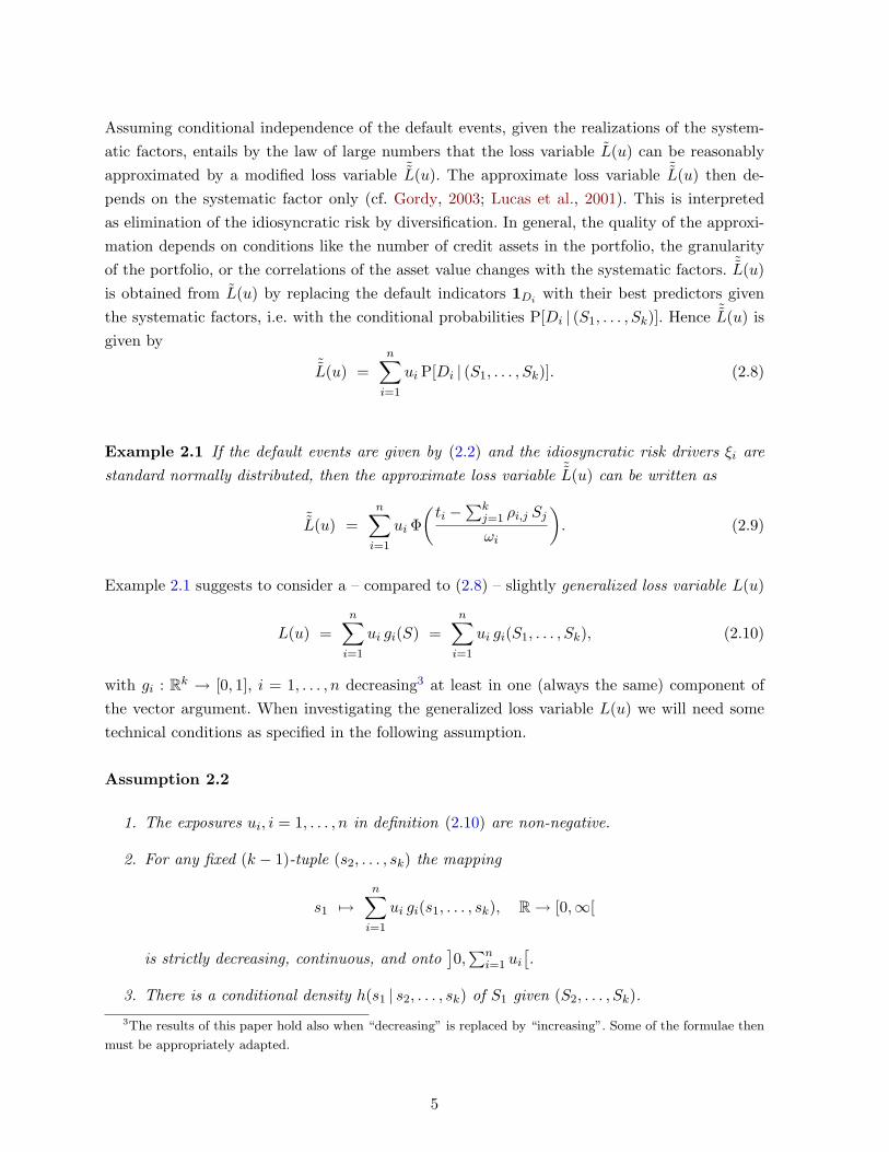
In order to assess the impact of factor diversification at portfolio level, first we calculate11 VaR­figures at different levels both for the single factor model as in (5.3) with w = 1 as well as for the

two factor model with w = 0. Table 1 shows that the impact even in the case of an independent second factor and for high levels of VaR remains limited.

This picture changes dramatically if we consider UL contributions with respect to VaR instead

of total UL. “UL” means “unexpected loss” and is defined by choosing

�(V ) = VaRα(V ) − E[V ] = qα(V ) − E[V ] = UL(V ) (5.5)

in Definition 3.1. In Figure 1 we plot the relative contribution to UL with respect to 99.9%­VaR

of the first asset in the model in Example 5.1 against the extent of the asset’s exposure to the

first factor (low values of w correspond to low exposure, values of w close to 1 correspond to high

exposure). It turns out that the size of the risk contribution of the first asset can be reduced

The more intricate calculations for this paper were conducted by means of the statistics software package R

(cf. R Development Core Team, 2003).

16

11

� �

�

� � �

Assuming conditional independence of the default events, given the realizations of the system­atic factors, entails by the law of large numbers that the loss variable L(u) can be reasonably

approximated by a modified loss variable ˜ L(u) then de­L(u). The approximate loss variable ˜

pends on the systematic factor only (cf. Gordy, 2003; Lucas et al., 2001). This is interpreted

as elimination of the idiosyncratic risk by diversification. In general, the quality of the approxi­mation depends on conditions like the number of credit assets in the portfolio, the granularity

of the portfolio, or the correlations of the asset value changes with the systematic factors. ˜L(u) is obtained from L(u) by replacing the default indicators 1Di with their best predictors given

the systematic factors, i.e. with the conditional probabilities P[Di | (S1, . . . , Sk )]. Hence ˜L(u) is given by

n˜ � L(u) = ui P[Di | (S1, . . . , Sk )]. (2.8)

i=1

Example 2.1 If the default events are given by (2.2) and the idiosyncratic risk drivers ξi are

standard normally distributed, then the approximate loss variable ˜L(u) can be written as

n � �k � ˜L(u) =

� ui Φ

ti − j=1 ρi,j Sj . (2.9)

ωii=1

Example 2.1 suggests to consider a – compared to (2.8) – slightly generalized loss variable L(u)

n n

L(u) = ui gi(S) = ui gi(S1, . . . , Sk ), (2.10) i=1 i=1

with gi : Rk → [0, 1], i = 1, . . . , n decreasing3 at least in one (always the same) component of the vector argument. When investigating the generalized loss variable L(u) we will need some

technical conditions as specified in the following assumption.

Assumption 2.2

1. The exposures ui, i = 1, . . . , n in definition (2.10) are non­negative.

2. For any fixed (k − 1)­tuple (s2, . . . , sk ) the mapping

n

s1 ui gi(s1, . . . , sk ), R → [0,∞[�→ i=1

nis strictly decreasing, continuous, and onto 0, .i=1 ui

3. There is a conditional density h(s1 | s2, . . . , sk ) of S1 given (S2, . . . , Sk ).

The results of this paper hold also when “decreasing” is replaced by “increasing”. Some of the formulae then

must be appropriately adapted.

5

3

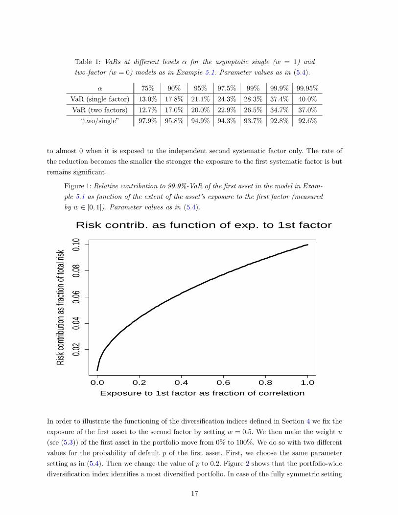
Table 1: VaRs at different levels α for the asymptotic single (w = 1) and

two­factor (w = 0) models as in Example 5.1. Parameter values as in (5.4).

α 75% 90% 95% 97.5% 99% 99.9% 99.95%

VaR (single factor) 13.0% 17.8% 21.1% 24.3% 28.3% 37.4% 40.0%

VaR (two factors) 12.7% 17.0% 20.0% 22.9% 26.5% 34.7% 37.0%

“two/single” 97.9% 95.8% 94.9% 94.3% 93.7% 92.8% 92.6%

to almost 0 when it is exposed to the independent second systematic factor only. The rate of the reduction becomes the smaller the stronger the exposure to the first systematic factor is but remains significant.

Figure 1: Relative contribution to 99.9%­VaR of the first asset in the model in Exam­ple 5.1 as function of the extent of the asset’s exposure to the first factor (measured

by w ∈ [0, 1]). Parameter values as in (5.4).

0.0 0.2 0.4 0.6 0.8 1.0

0.02

0.04

0.06

0.08

0.10

Exposure to 1st factor as fraction of correlation

Risk

contr

ibutio

n as f

racti

on of

total

risk

Risk contrib. as function of exp. to 1st factor

In order to illustrate the functioning of the diversification indices defined in Section 4 we fix the

exposure of the first asset to the second factor by setting w = 0.5. We then make the weight u

(see (5.3)) of the first asset in the portfolio move from 0% to 100%. We do so with two different values for the probability of default p of the first asset. First, we choose the same parameter setting as in (5.4). Then we change the value of p to 0.2. Figure 2 shows that the portfolio­wide

diversification index identifies a most diversified portfolio. In case of the fully symmetric setting

17

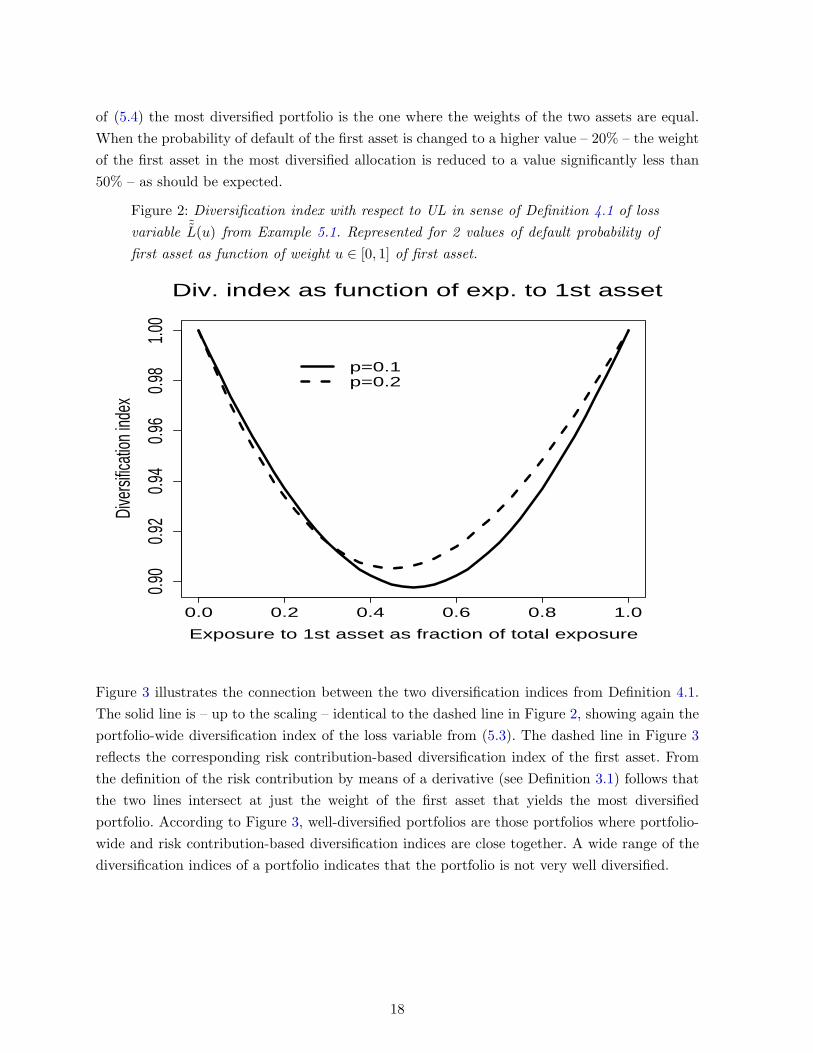
of (5.4) the most diversified portfolio is the one where the weights of the two assets are equal. When the probability of default of the first asset is changed to a higher value – 20% – the weight of the first asset in the most diversified allocation is reduced to a value significantly less than

50% – as should be expected.

Figure 2: Diversification index with respect to UL in sense of Definition 4.1 of loss

variable ˜L(u) from Example 5.1. Represented for 2 values of default probability of first asset as function of weight u ∈ [0, 1] of first asset.

0.0 0.2 0.4 0.6 0.8 1.0

0.90

0.92

0.94

0.96

0.98

1.00

Exposure to 1st asset as fraction of total exposure

Dive

rsific

ation

inde

x

Div. index as function of exp. to 1st asset

p=0.1p=0.2

Figure 3 illustrates the connection between the two diversification indices from Definition 4.1. The solid line is – up to the scaling – identical to the dashed line in Figure 2, showing again the

portfolio­wide diversification index of the loss variable from (5.3). The dashed line in Figure 3

reflects the corresponding risk contribution­based diversification index of the first asset. From

the definition of the risk contribution by means of a derivative (see Definition 3.1) follows that the two lines intersect at just the weight of the first asset that yields the most diversified

portfolio. According to Figure 3, well­diversified portfolios are those portfolios where portfolio­wide and risk contribution­based diversification indices are close together. A wide range of the

diversification indices of a portfolio indicates that the portfolio is not very well diversified.

18

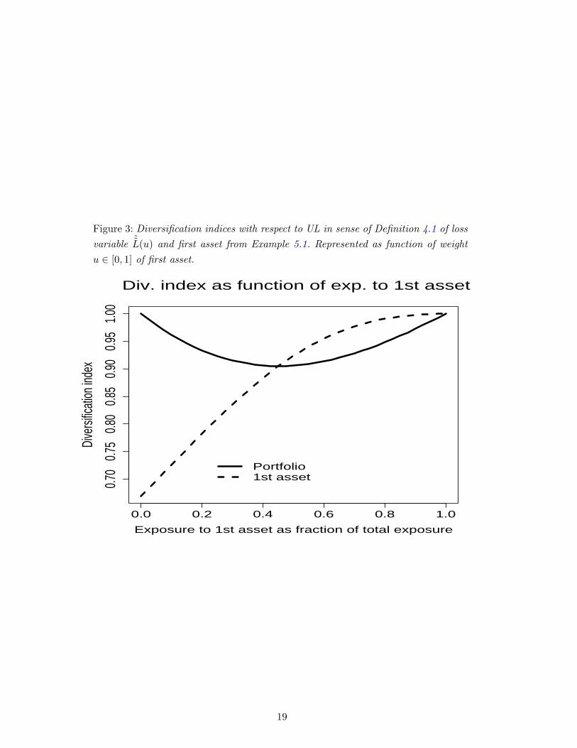
Figure 3: Diversification indices with respect to UL in sense of Definition 4.1 of loss

variable ˜L(u) and first asset from Example 5.1. Represented as function of weight u ∈ [0, 1] of first asset.

0.0 0.2 0.4 0.6 0.8 1.0

0.70

0.75

0.80

0.85

0.90

0.95

1.00

Exposure to 1st asset as fraction of total exposure

Dive

rsific

ation

inde

x

Div. index as function of exp. to 1st asset

Portfolio1st asset

19

6 Conclusions

In this paper we have derived explicit formulae for risk contributions to VaR and ES in the

context of asymptotic multi­factor models, thus generalizing the capital requirements as provided

by the Basel II Accord in the context of the ASRF (Asymptotic Single Risk Factor) model. The

effort needed for the numerical calculations is higher than in the ASRF case but, as a numerical example shows, remains feasible at least in the case of two­factor models. The example also

indicates that the effect of factor diversification on portfolio­wide economic capital is moderate

but can be significant for risk contributions of single assets or sub­portfolios.

The risk contributions we analyze in the first sections of the paper can be used for calculating

diversification indices for sub­portfolios or assets in a portfolio. If these indices, considered for all the assets in the portfolio, take a wide range, then there is a high potential for diversification

in the portfolio. If, in contrast, the range of the indices is narrow, there is no potential left for diversification by changing the weights of the assets in the portfolio. In this case, more

diversification can be only reached by adding new assets or by removing assets from the portfolio.

This observation suggests the use of the newly developed diversification indices for reflecting

factor diversification: assets found well­diversified by an index close to the portfolio­wide index

could receive a reduction of capital requirements. The sizes of such reductions could be estimated

by means of an asymptotic two­factor model. Of course, the concrete choice of the model and

its underlying parameters might have a strong impact on the estimates. Further research in this direction seems necessary.

References

Acerbi, C. and D. Tasche (2002) On the coherence of Expected Shortfall. Journal of Banking and Finance 26(7), 1487­1503.

Basel Committee on Banking Supervision (BCBS) (2004) Basel II: International Con­vergence of Capital Measurement and Capital Standards: a Revised Framework. http://www.bis.org/publ/bcbs107.htm

Bluhm, C., Overbeck, L. and C. Wagner (2002) An Introduction to Credit Risk Modeling. CRC Press: Boca Raton.

Denault, M. (2001) Coherent allocation of risk capital. Journal of Risk 4(1), 1­34.

Embrechts, P., Hoing, A. and A. Juri (2003) Using Copulae to bound the Value­at­Risk

for functions of dependent risks. Finance & Stochastics 7(2), 145­167.

Emmer, S. and D. Tasche (2005) Calculating Credit Risk Capital Charges with the One­Factor Model. Journal of Risk 7(2), 85­101.

20

Garcia Cespedes, J. C., Kreinin, A. and D. Rosen (2004) A Simple Multi­Factor “Factor Adjustment” for the Treatment of Diversification in Credit Capital Rules. Working paper, BBVA and Algorithmics Inc.

Gordy, M. (2003) A Risk­Factor Model Foundation for Ratings­Based Bank Capital Rules. Journal of Financial Intermediation 12(3), 199­232.

Gourieroux, C., Laurent, J. P. and O. Scaillet (2000) Sensitivity analysis of Values at Risk. Journal of Empirical Finance, 7, 225­245.

Kalbrener, M. (2005) An axiomatic approach to capital allocation. Mathematical Finance

15(3), 425­437.

Kalbrener, M., Lotter, H. and L. Overbeck (2004) Sensible and efficient capital allo­cation for credit portfolios. Risk 17(1), S19­S24.

Lemus, G. (1999) Portfolio Optimization with Quantile­based Risk Measures. PhD thesis, Sloan

School of Management, MIT. http://citeseer.ist.psu.edu/lemus99portfolio.html

Litterman, R. (1996) Hot SpotsTM and Hedges. The Journal of Portfolio Management 22, 52­75.

Lucas, A., Klaassen, P., Spreij, P. und S. Straetmans (2001) An analytic approach

to credit risk of large corporate bond and loan portfolios. Journal of Banking & Finance 25, 1635­1664.

Luciano, E. and M. Marena (2003) Value at risk bounds for portfolios of non­normal returns. In New Trends in Banking Management. C. Zopoudinis (ed.). Physica­Verlag, 207­222.

Martin, R. and D. Tasche (2005) CVaR: A Tale of Two Parts. Working paper.

Mausser, H. and D. Rosen (2004) Allocating Credit Capital with VaR Contributions. Working paper, Algorithmics Inc.

Memmel, C. and C. Wehn (2005) The supervisor’s portfolio: the market price risk of German

banks from 2001 to 2003 – Analysis and models for risk aggregation. Discussion Paper Series 2: Banking and Financial Studies No 02/2005, Deutsche Bundesbank. http://www.bundesbank.de/bankenaufsicht/bankenaufsicht diskussionspapiere.en.php

Patrik, G., Bernegger, S. and M.B. Ruegg (1999) The use of risk adjusted capital to

support business decision­making. CAS Forum 1999 Spring, Reinsurance Call Papers. http://www.casact.org/pubs/forum/99spforum/99spftoc.htm

Pykhtin, M. (2004) Multi­factor adjustment. Risk 17(3), 85­90.

21

R Development Core Team (2003) R: A language and environment for statistical comput­ing. R Foundation for Statistical Computing, Vienna. http://www.R­project.org

Tasche, D. (1999) Risk contributions and Performance Measurement. Working paper, Tech­nische Universit¨ unchen.at M¨

Tasche, D. (2002) Expected Shortfall and Beyond. Journal of Banking and Finance 26(7), 1519­1533.

22