RISK FACTORS ASSOCIATED WITH HIGH … FACTORS ASSOCIATED WITH HIGH POTENTIAL FOR SERIOUS CRASHES Final ... Risk Factors Associated with High Potential for Serious ... (Veneziano …

RISK FACTORS ASSOCIATED WITH HIGH POTENTIAL FOR SERIOUS

CRASHES

Final Report

SPR 771

RISK FACTORS ASSOCIATED WITH HIGH POTENTIAL FOR SERIOUS CRASHES

Final Report

SPR 771

by Ahmed Al-Kaisy, PhD, PE – Professor & Program Manager

David Veneziano, PhD – Research Scientist II Levi Ewan, PE – Research Engineer

Fahmid Hossain – Graduate Research Assistant

Western Transportation Institute Montana State University

Bozeman, MT 59717-4250

for

Oregon Department of Transportation Research Section

555 13th Street NE, Suite 1 Salem OR 97301

and

Federal Highway Administration 400 Seventh Street, SW

Washington, DC 20590-0003

September 2015

i

Technical Report Documentation Page

1. Report No.

FHWA-OR-RD-16-05

2. Government Accession No. 3. Recipient’s Catalog No.

4. Title and Subtitle

Risk Factors Associated with High Potential for Serious Crashes

5. Report Date

September 2015

6. Performing OrganizationCode

7. Author(s)Ahmed Al-Kaisy, Levi Ewan, David Veneziano, and Fahmid Hossain

8. Performing OrganizationReport No.

9. Performing Organization Name and AddressWestern Transportation Institute

Montana State University P.O. Box 174250 Bozeman, MT 59717-4250

10. Work Unit No. (TRAIS)

11. Contract or Grant No.

SPR 771

12. Sponsoring Agency Name and Address

Oregon Dept. of TransportationResearch Section and Federal Highway Admin. 555 13th Street NE, Suite 1 400 Seventh Street, SWSalem, OR 97301 Washington, DC 20590-0003

13. Type of Report and PeriodCovered

Final Report

14. Sponsoring Agency Code

15. Supplementary Notes

16. Abstract

Crashes are random events and low traffic volumes therefore don’t always make crash hot-spot identification possible. This project has used extensive data collection and analysis for a large sample of Oregon’s low volume roads to develop a risk index that expresses the crash risk for different road geometries and roadside features as well as crash history and traffic exposure. This crash risk index can then be a proactive means of identifying potentially risky locations where safety treatments might be best targeted. The economic analysis completed as part of this effort can be used in conjunction with the risk index when determining which safety treatments may result in the highest return on investment for agency safety improvement funds. This report includes a review of literature related to features effecting crash risk and other past risk index efforts, the data collection and analysis methods used in quantifying risks, the establishment of the crash risk index, an economic feasibility analysis showing which treatments may be the best options for Oregon’s low volume roads, and a few case studies highlighting the use of the crash risk index on three samples of Oregon’s low volume roadways.

17. Key WordsCrash risk, low volume road, risk factor,countermeasures, risk index

18. Distribution Statement

Copies available from NTIS, and online at http://www.oregon.gov/ODOT/TD/TP_RES/

19. Security Classification(of this report)

Unclassified

20. Security Classification(of this page)

Unclassified

21. No. of Pages

157

22. Price

Technical Report Form DOT F 1700.7 (8-72) Reproduction of completed page authorized Printed on recycled paper

ii

iii

SI* (MODERN METRIC) CONVERSION FACTORS

APPROXIMATE CONVERSIONS TO SI UNITS APPROXIMATE CONVERSIONS FROM SI UNITS

Symbol When You

Know Multiply

By To Find Symbol Symbol

When You Know

Multiply By

To Find Symbol

LENGTH LENGTH

in inches 25.4 millimeters mm mm millimeters 0.039 inches in ft feet 0.305 meters m m meters 3.28 feet ft yd yards 0.914 meters m m meters 1.09 yards yd mi miles 1.61 kilometers km km kilometers 0.621 miles mi

AREA AREA

in2 square inches 645.2 millimeters squared

mm2 mm2 millimeterssquared

0.0016 square inches in2

ft2 square feet 0.093 meters squared m2 m2 meters squared 10.764 square feet ft2 yd2 square yards 0.836 meters squared m2 m2 meters squared 1.196 square yards yd2 ac acres 0.405 hectares ha ha hectares 2.47 acres ac

mi2 square miles 2.59 kilometers squared

km2 km2 kilometerssquared

0.386 square miles mi2

VOLUME VOLUME

fl oz fluid ounces 29.57 milliliters ml ml milliliters 0.034 fluid ounces fl oz gal gallons 3.785 liters L L liters 0.264 gallons gal ft3 cubic feet 0.028 meters cubed m3 m3 meters cubed 35.315 cubic feet ft3 yd3 cubic yards 0.765 meters cubed m3 m3 meters cubed 1.308 cubic yards yd3

NOTE: Volumes greater than 1000 L shall be shown in m3.

MASS MASS

oz ounces 28.35 grams g g grams 0.035 ounces oz lb pounds 0.454 kilograms kg kg kilograms 2.205 pounds lb

T short tons (2000 lb)

0.907 megagrams Mg Mg megagrams 1.102 short tons (2000 lb) T

TEMPERATURE (exact) TEMPERATURE (exact)

°F Fahrenheit (F-32)/1.8

Celsius °C °C Celsius 1.8C+32

Fahrenheit °F

*SI is the symbol for the International System of Measurement

iv

v

ACKNOWLEDGEMENTS

The authors wish to thank the Oregon Department of Transportation and the Federal Highway Administration for the funding of this research. They also wish to thank the project technical advisory committee, including Mark Joerger, Douglas Bish, Timothy Burks, Kevin Haas, Nick Fortey, Amanda Salyer, and Zahidul Siddique for their input and assistance in this work. Finally, they thank Janice Simmons formerly of the Western Transportation Institute for her assistance in the data collection portion of this work.

DISCLAIMER

This document is disseminated under the sponsorship of the Oregon Department of Transportation and the United States Department of Transportation in the interest of information exchange. The State of Oregon and the United States Government assume no liability of its contents or use thereof.

The contents of this report reflect the view of the authors who are solely responsible for the facts and accuracy of the material presented. The contents do not necessarily reflect the official views of the Oregon Department of Transportation or the United States Department of Transportation.

The State of Oregon and the United States Government do not endorse products of manufacturers. Trademarks or manufacturers’ names appear herein only because they are considered essential to the object of this document.

This report does not constitute a standard, specification, or regulation.

vi

vii

TABLE OF CONTENTS

1.0 INTRODUCTION............................................................................................................. 1

2.0 LITERATURE REVIEW ................................................................................................ 3

2.1 LOW-VOLUME ROADS AND RISK FACTORS ........................................................................ 3 2.1.1 Low-Volume Roads ................................................................................................................................ 3 2.1.2 Risk Factors ........................................................................................................................................... 3

2.1.2.1 Roadside ............................................................................................................................................................ 3 2.1.2.2 Cross Section ..................................................................................................................................................... 5 2.1.2.3 Alignment ......................................................................................................................................................... 8

2.1.3 Summary of Identified Risk Factors ....................................................................................................... 9 2.2 LOW-COST COUNTERMEASURES TO MITIGATE RISK ........................................................ 10

2.2.1 Alignment ............................................................................................................................................. 10 2.2.1.1 Curve Delineation ........................................................................................................................................... 11 2.2.1.2 Curve Warning Pavement Markings ............................................................................................................... 11 2.2.1.3 Curve Warning Signs ...................................................................................................................................... 12

2.2.2 Road Cross Section .............................................................................................................................. 13 2.2.2.1 Lane Widening ................................................................................................................................................ 13 2.2.2.2 Pavement Friction ........................................................................................................................................... 14 2.2.2.3 Shoulder Improvements .................................................................................................................................. 14

2.2.3 Roadside Features ............................................................................................................................... 15 2.2.3.1 Clear Zone Improvements ............................................................................................................................... 15 2.2.3.2 Flattening Side Slopes ..................................................................................................................................... 15 2.2.3.3 Prevent Pavement Edge Drops ........................................................................................................................ 16

2.2.4 Other Measures ................................................................................................................................... 16 2.2.4.1 Centerline and Edge-line Marking Improvements ........................................................................................... 16 2.2.4.2 Centerline and Edge-line rumble Strips / Stripes............................................................................................. 17 2.2.4.3 Lighting Improvements ................................................................................................................................... 18 2.2.4.4 Other Warning Signs ....................................................................................................................................... 18 2.2.4.5 Transverse Lane Markings and Warnings ....................................................................................................... 19 2.2.4.6 Transverse Rumble Strips ............................................................................................................................... 19

2.2.5 Countermeasure Effectiveness and Benefit/Cost ................................................................................. 20 2.2.5.1 Alignment Countermeasures Effectiveness ..................................................................................................... 20 2.2.5.2 Road Cross-Section Countermeasures Effectiveness ...................................................................................... 24 2.2.5.3 Roadside Features Countermeasures ............................................................................................................... 31 2.2.5.4 Other Countermeasures Effectiveness ............................................................................................................. 34

2.3 EXISTING RISK AND SAFETY INDICES .............................................................................. 42 2.3.1 Existing Approaches ............................................................................................................................ 42 2.3.2 Summary of Existing Risk Indices ........................................................................................................ 49

2.4 LITERATURE REVIEW SUMMARY ..................................................................................... 49

3.0 DATA COLLECTION ................................................................................................... 52

3.1 SAMPLE SELECTION ........................................................................................................ 52 3.2 DATA SOURCES AND GATHERING .................................................................................... 53

4.0 DATA ANALYSIS .......................................................................................................... 55

4.1 METHODS ....................................................................................................................... 55 4.2 OREGON’S LOW VOLUME ROADS: CHARACTERISTICS AND CRASHES ............................... 55

4.2.1 Road Characteristics ........................................................................................................................... 55 4.2.2 Overall Crash Characteristics ............................................................................................................. 58

4.3 CRASH OCCURRENCE AND ROAD CHARACTER RELATIONSHIPS ....................................... 60 4.3.1 Lane Width ........................................................................................................................................... 60 4.3.2 Shoulder Width .................................................................................................................................... 63

viii

4.3.3 Grade ................................................................................................................................................... 64 4.3.4 Side Slope ............................................................................................................................................ 66 4.3.5 Fixed Objects in Clear Zone ................................................................................................................ 68 4.3.6 Driveway Density ................................................................................................................................. 70 4.3.7 Horizontal Curves ................................................................................................................................ 72 4.3.8 Vertical Curves .................................................................................................................................... 76

4.4 REGRESSION AND CORRELATION .................................................................................... 78 4.4.1 Crash Rate Regression ......................................................................................................................... 79 4.4.2 Crash Severity Rate Regression ........................................................................................................... 80 4.4.3 Correlation Analysis ............................................................................................................................ 81

4.5 DATA ANALYSIS SUMMARY ............................................................................................ 81

5.0 RISK INDEX DEVELOPMENT .................................................................................. 83

5.1 GENERAL FORM .............................................................................................................. 83 5.2 GEOMETRIC FEATURES ................................................................................................... 84

5.2.1 Geometric Feature Weights ................................................................................................................. 84 5.2.2 Geometric Feature Values ................................................................................................................... 86

5.3 CRASH HISTORY ............................................................................................................. 88 5.4 TRAFFIC EXPOSURE ........................................................................................................ 89 5.5 RISH INDEX DEVELOPMENT SUMMARY ........................................................................... 90

6.0 ECONOMIC FEASIBILITY ......................................................................................... 91

6.1 ROAD SAMPLE ................................................................................................................ 91 6.2 SAFETY COUNTERMEASURES .......................................................................................... 91 6.3 BENEFIT-COST ANALYSIS ................................................................................................ 93

6.3.1 Costs of Countermeasures ................................................................................................................... 94 6.3.2 Benefits of Countermeasures ............................................................................................................... 98 6.3.3 Benefit / Cost Relationships ............................................................................................................... 102

6.4 ECONOMIC ANALYSIS CONCLUSIONS ............................................................................ 105

7.0 CASE STUDIES ............................................................................................................ 107

7.1 STUDY SITES AND METHODOLOGY ............................................................................... 107 7.2 RESULTS ...................................................................................................................... 108

8.0 SUMMARY ................................................................................................................... 111

9.0 REFERENCES .............................................................................................................. 114

LIST OF TABLES

Table 2.1:Evaluations of Countermeasures Mitigating for Alignment Risk Factors ................................................... 21 Table 2.2: Evaluations of Countermeasures Mitigating for Road Cross-Section Related Risk Factors ...................... 24 Table 2.3: Results from Evaluations of Countermeasures Mitigating for Risk Factors related to Roadside Features . 31 Table 2.4: Results from Evaluations of Countermeasures Mitigating for Risk Factors related to Other Features Not

Included in the Previous Sections. ..................................................................................................................... 34 Table 4.1: Region Comparison .................................................................................................................................... 60 Table 4.2: Summary of Crash Rate Regression Results .............................................................................................. 79 Table 4.3: Summary of Crash Severity Rate Regression Results ................................................................................ 80 Table 4.4: Correlation Results ..................................................................................................................................... 81

ix

Table 4.5: Road Character Summary ........................................................................................................................... 82 Table 5.1: Overall Geometric Features Weights .......................................................................................................... 85 Table 5.2: Equations for Geometric and Roadside Features ........................................................................................ 87 Table 5.3: Traffic Exposure Values ( ) .................................................................................................................... 90 Table 6.1: Sample Crash Rates by Crash Type ............................................................................................................ 91 Table 6.2: Costs of Alignment Safety Measures ......................................................................................................... 95 Table 6.3: Costs of Roadway Cross Section Safety Measures..................................................................................... 96 Table 6.4: Costs of Roadside Features Safety Measures ............................................................................................. 97 Table 6.5: Costs of Other Safety Measures ................................................................................................................. 98 Table 6.6: Benefits of Alignment Safety Measures ..................................................................................................... 99 Table 6.7: Benefits of Roadway Cross Section Safety Measures .............................................................................. 100 Table 6.8: Benefits of Roadside Features Safety Measures ....................................................................................... 101 Table 6.9: Benefits of Other Safety Measures ........................................................................................................... 101 Table 6.10: Crash Costs ............................................................................................................................................. 102 Table 6.11: Estimated Crash Costs on Road Sample ................................................................................................. 102 Table 6.12: Benefit/Costs Ratios of Alignment Safety Measures .............................................................................. 103 Table 6.13: Benefit/Costs Ratios of Roadway Cross Section Safety Measures ......................................................... 104 Table 6.14: Benefit/Costs Ratios of Roadside Features Safety Measures ................................................................. 104 Table 6.15: Benefit/Costs Ratios of Other Safety Measures...................................................................................... 105

LIST OF FIGURES

Figure 2.1: Curve Delineation Examples (a, b, c - (McGee and Hanscom 2006); d - (FHWA 2012); e - (FHWA 2013)) ................................................................................................................................................................. 11

Figure 2.2: Curve Warning Pavement Marking Examples (a –(ATSSA 2006), b – (Hallmark et al. 2013a)) ............. 12 Figure 2.3: Curve Warning Sign Examples (a, b – (Hallmark et al. 2013a); c, d – (McGee and Hanscom 2006)) .... 13 Figure 2.4: Pavement Friction Improvement Measures (a – (Veneziano and Villwock-Witte 2013), b – (Veneziano et

al. 2011) ............................................................................................................................................................. 14 Figure 2.5: Example of Road that may Benefit from Shoulder Improvements (Sun and Das 2012) ........................... 15 Figure 2.6: Example of Pavement Edge Drop (Kirk 2008) .......................................................................................... 16 Figure 2.7: Example of Centerline and Shoulder Rumble Strips (a – (Datta et al. 2012), b - WTI) ........................... 17 Figure 2.8: Example of other Dynamic Warning Signs (a – (Hallmark et al. 2013d), b – (Simpson and Troy 2012))18 Figure 2.9: Example of Transverse Lane Markings and Warnings (a – (Arnold and Lantz 2007), b – (Gross et al.

2008)) ................................................................................................................................................................. 19 Figure 2.10: Example of Transverse Rumble Strips (a – (Fitzpatrick et al. 2003), b – (Harder et al. 2006)) ............. 20 Figure 3.1: Sample Definition (Map Source: Google Maps) ....................................................................................... 53 Figure 4.1: Sample Lane and Shoulder Widths ........................................................................................................... 56 Figure 4.2: Sample AADT Ranges and Driveway Densities ....................................................................................... 56 Figure 4.3: Sample Fixed Object and Side Slope Ratings ........................................................................................... 57 Figure 4.4: Sample Degree of Curvature ..................................................................................................................... 57 Figure 4.5: Sample Horizontal and Vertical Curve Lengths ........................................................................................ 58 Figure 4.6: Sample Grade Distribution ........................................................................................................................ 58 Figure 4.7: Crash Types and Vehicle Involvement ..................................................................................................... 59 Figure 4.8: Crash Severity and Driver Age Involvement ............................................................................................ 59 Figure 4.9: Distance from Home and Day of Week .................................................................................................... 60 Figure 4.10: Crash Rate by Lane Width ...................................................................................................................... 61 Figure 4.11: Crash Characteristics by Lane Width ...................................................................................................... 62 Figure 4.12: Crash Rate by Shoulder Width ................................................................................................................ 63 Figure 4.13: Crash Characteristics by Shoulder Width................................................................................................ 64 Figure 4.14: Crash Rate by Percent Grade .................................................................................................................. 65 Figure 4.15: Crash Characteristics by Percent Grade .................................................................................................. 66 Figure 4.16: Crash Rate by Side Slope Rating ............................................................................................................ 67 Figure 4.17: Crash Characteristics by Side Slope Rating ............................................................................................ 68

x

Figure 4.18: Crash Rate by Fixed Object Rating ......................................................................................................... 69 Figure 4.19: Crash Characteristics by Fixed Object Rating ......................................................................................... 70 Figure 4.20: Crash Rate by Driveway Density ............................................................................................................ 71 Figure 4.21: Crash Characteristics by Driveway Density ............................................................................................ 72 Figure 4.22: Crash Rate by Degree of Curvature ........................................................................................................ 73 Figure 4.23: Crash Characteristics by Degree of Curvature ........................................................................................ 74 Figure 4.24: Crash Rate by Length of Horizontal Curve ............................................................................................. 75 Figure 4.25: Crash Characteristics by Length of Horizontal Curve ............................................................................. 76 Figure 4.26: Crash Rate by Length of Vertical Curve ................................................................................................. 77 Figure 4.27: Crash Characteristics by Length of Vertical Curve ................................................................................. 78 Figure 5.1: Geometric Feature Value for Degree of Curvature ................................................................................... 86 Figure 5.2: XG Definition............................................................................................................................................. 88 Figure 5.3: Crash History Value .................................................................................................................................. 89 Figure 7.1: Case Study Sites (Map Source: ODOT TransGIS System & ESRI) ....................................................... 107 Figure 7.2: Highway 171 Sliding One-Mile CRI and Crash Rate ............................................................................. 108 Figure 7.3: Highway 036 Sliding One-Mile CRI and Crash Rate ............................................................................. 109 Figure 7.4: Highway 380 Sliding One-Mile CRI and Crash Rate ............................................................................. 110

1

1.0 INTRODUCTION

Crashes are random events and consequently, can occur at any location along the roadway. On roadways with higher traffic volumes, the more frequent occurrence of crashes allows for the direct identification of high crash locations using historical data. However, on local roads, crash occurrence, particularly fatal and serious injury crashes, is less frequent. This makes it difficult to identify trends and treat hazardous sites based on historical data. Geometric, traffic and other features may lend themselves toward crashes potentially happening in spot locations. Therefore, an approach to identifying these types of risk factors on low volume roads is necessary. It is imperative to identify, develop and deliver such approaches for low-volume roads, both those operated by the Oregon Department of Transportation and local agencies (for example, counties), in order to reduce the number and severity of highway crashes and improve highway safety.

In essence, the identification of such features and sites is a proactive approach to identifying locations where potential safety issues may exist but no/few crashes may have occurred to date. In identifying such sites, low cost safety countermeasures could then be applied, either at a limited number of locations or on a systemic basis, depending on identified concerns and needs as well as available budget. This proactive approach can prevent or reduce the severity of crashes without waiting for a critical mass of such crashes to occur prior to identifying improvement locations. In many cases, the improvements that can be made are low cost, which creates an opportunity to produce substantial benefits for a relatively small investment. As a result, safety is improved on roadways that are often given lower priority or consideration given the traffic volumes they serve.

There is a need to better understand the different risks associated with factors and features along low- and moderate-volume roadways. In understanding where risks are present in the system, a proactive or reactive approach may be employed to make improvements that can translate into reduced (or prevented) crashes in the future. To an extent, such an approach would be similar to a Road Safety Audit (RSA) in that it seeks to identify potential safety issues before they contribute to crashes or based on the occurrence of a significant number of crashes at a location. In Oregon, RSA are used as a reactive tool for crashes. RSAs are limited in that they typically focus on one roadway segment of a finite length due to time, cost and labor constraints and require field site visits. Consequently, similar features or factors that can contribute to crashes along other segments can typically go unidentified. As a result, the systemic implementation of an improvement to address those features or factors is not achieved.

Six major tasks have been completed to address these needs including 1) conducting a Literature Review to understand existing approaches and previously identified risk factors and features, 2) Collecting Data for a large sample of Oregon’s low-volume roads, 3) performing Data Analysis to understand what features may influence crash risk, 4) Developing a Risk Index that provides a means to quantify crash risk based on roadway and traffic characteristics, 5) investigating Economic Feasibility to determine which low-cost safety measures may be the best use of the agency safety improvement funds, and 6) performing Case Studies to illustrate how the risk

2

index can be used with real-world data from samples of Oregon’s low-volume roads. The following chapters will detail each of these tasks and the findings and results produced with each effort.

3

2.0 LITERATURE REVIEW

In order to develop an approach to identifying risk factors on low volume roads, it is necessary to first understand what approaches may exist, as well as what factors and features have been identified as presenting a risk in previous studies. The literature review presented in the following sections develops such an understanding.

2.1 LOW-VOLUME ROADS AND RISK FACTORS

2.1.1 Low-Volume Roads

Low-volume roads comprise a significant portion of roadway mileage in the U.S. However, the definition of what constitutes a low-volume road can vary. The Manual on Uniform Traffic Control Devices (MUTCD) states in Chapter 5A that “A low-volume road shall be a facility lying outside of built-up areas of cities, towns, and communities, and it shall have a traffic volume of less than 400 AADT [Annual Average Daily Traffic]” (FHWA 2009). Alternatively, Chapter 2 of the MUTCD, specifically Section 2C.06 which pertains to horizontal alignment warning signs, establishes a cutoff between high and low volume roads of 1,000 AADT (FHWA 2009). Work by Iowa State University produced a similar 400 vehicle per day (vpd) value when defining low-volume roads (McDonald and Sperry 2013). Gross et al. (Gross et al. 2011) cite a figure of 1,000 vehicles per day as constituting low-volume roads and less than 400 VPD for very low-volume roads.

As many of the references presented in the following text indicate, the threshold of 400 to 500 vehicles per day is a fairly common measure of a low-volume road. In some cases, higher figures are used, reaching the point of 1,000 vpd similar to what is identified above. For the purpose of the current project, it is reasonable to employ the higher threshold MUTCD guidance of 1,000 vpd or lower AADT as an appropriate traffic level to consider as a low-volume road.

2.1.2 Risk Factors

Researchers have extensively focused on identifying the different factors and features of roadways that contribute to crashes. In a low volume, rural context, this includes work examining roadway aspects such as lane and shoulder widths, curve radius, intersection control, pavement markings, lateral clearance, side slope condition, driveway density and grades. The literature in the following sections establishes the specific features and factors that pose a risk for serious crashes on rural roads and the extent to which they have impacted safety.

2.1.2.1 Roadside

As part of developing a roadside hazardousness index, Pardillo-Mayora et al. (Pardillo-Mayora et al. 2010) focused on four roadside features that influenced the results of road

4

departure crashes. These included roadside slope, distance from the roadside edge to obstacles, barrier presence and horizontal alignment. These features were selected based on previous research results and no values associated with the risks they pose were provided by this work.

Bendigeri et al. (Bendigeri et al. 2011) identified factors contributing to roadside tree crashes on different classes of roads in South Carolina. Approximately 48 percent of tree crashes in the state occurred on secondary routes, with drivers under the age of 36 involved in over 57 percent of those crashes. Using laser scan data of the roadside, it was determined that 48 of the 51 study sites that had experienced a crash did not meet clear zone requirements. Specifically, critical side slopes and non-traversable ditches reduced effective clear zone distances.

Cafiso et al. (Cafiso et al. 2010), in discussing the cost effectiveness of safety countermeasures on rural two lane roads in Italy, listed safety issues and their percentage increase in safety risk. Roadway geometry issues were found to increase crash risk by 700 percent. Deficiencies in other areas also increased safety risks, including driveway presence by 135 percent, delineation by 30 percent, markings by 20 percent, pavement by 10 percent, roadside features by 200 percent, sight distance by 50 percent and signage by 20 percent. As these figures indicate, various aspects of the rural roadway environment individually or in combination can present significant safety risks.

Schrum et al. (Schrum et al. 2012) undertook a field study of low volume roads in Kansas and Nebraska to identify common fixed objects and geometric features that presented safety issues to drivers. Features identified by this effort included culverts, bridges, driveways, trees, ditches, slopes, utility poles and public broadcast service routing stations. Infrequent obstacles, including road and advertising signs, mailboxes, tree stumps, bushes, rock walls, boulders and water bodies were also identified as presenting issues. The Roadside Safety Analysis Program (RSAP) was used to determine impact frequencies and treatment options for these features based on measurements made in the course of the field study. The risks associated with the features identified by this work were not quantified however.

Souleyrette et al. (Souleyrette et al. 2010) performed a safety analysis of low volume (400 vpd) rural roads in Iowa. Among the relevant findings of this work was that crashes on rolling and hilly terrain were more frequent than on flat terrain. Crashes were also more frequent during the night. Fixed object crashes involved culverts, ditches, embankments, trees and poles at a higher frequency on low volume roads compared to their higher volume counterparts. Finally, crashes occurred at higher frequencies at bridges, railroad crossings, driveways and T and Y configuration intersections, but at a lower frequency at four-way intersections.

Peng et al. (Peng et al. 2012) evaluated the effects of roadside features on single vehicle crashes on rural two lane roads in Texas. Results of the analysis showed that shoulder width, lateral clearance and sideslope condition had a significant effect on road departure crashes. Crash frequency and severity increased when lateral clearance or shoulder width decreased or when a steeper sideslope was present. As shoulder widths increased from

5

zero to 10 feet, the probability of an injury crash fell from 9.6 percent of total crashes to 7.1 percent. Similarly, as lateral clearance increased from 10 feet to 40 feet, the probability of an injury crash fell from 8.8 percent to 6.4 percent. Finally, as slopes flattened, injury crash probability fell from 11.1 percent to 9.9 percent.

2.1.2.2 Cross Section

Gross et al. (Gross et al. 2011) identified general issues on low volume roads that present safety risks. These issues included narrow lane widths between 8 and 10.5 feet, narrow or lack of paved shoulders, lack of turn lanes and pavement edge drop offs of greater than 2 inches. Note that these issues were identified during observations from Road Safety Audits as opposed to a statistical evaluation.

Gross and Jovanis (Gross and Jovanis 2007)examined the safety effectiveness of lane and shoulder widths on rural, two lane highway segments in Pennsylvania, including low volume segments (below 500 vehicles average daily traffic (ADT). Segment and crash data were evaluated using a matched case-control approach which paired case segments with control segments to compare safety. Conditional logistic regression was used to investigate the relationship between the outcome (crashes) and risk factors (lane and shoulder width). Results indicated that lane widths between 10 to 11.5 feet and greater than 13 feet were less safe than other lane widths (i.e. 12 feet). Interestingly, lane widths less than 10 feet indicated a lower crash risk, which contradicts the findings of other studies. Shoulder widths of 0 to 3 feet were found to increase crash risk, with that risk dropping as widths increased.

Ivan et al. (Ivan et al. 1999) identified differences in causality factors for single and multi-vehicle crashes on two lane roads. While the work did not specifically focus on low volume roads, its results are still of interest to this research. The research found that single vehicle crash rates decreased with increased traffic intensity, wider shoulder widths and longer sight distances. Multi-vehicle crash rates increased with the presence of signalized intersections and decreased shoulder widths.

Wang et al. compiled a review of the effects of road characteristics on safety (Wang et al. 2013). This effort found that past evaluation of the relationship between speed and crashes produced mixed results, with some studies finding increased speeds reduced safety while other studies found the opposite trend. Regarding road characteristics, the researchers noted past work had found roads with narrow lanes (less than 11.5 feet) and sharp horizontal curves had decreased numbers of crashes. Similarly, increased shoulder width and pavement improvements had also been shown to decrease crashes. While these findings were the result of previous studies on different types of roads, they offer insights into the factors that may present risk on low volume roads.

Garber and Kassebaum (Garber and Kassbaum 2008) identified causal factors of crashes for high risk locations on rural and urban two lane roads in Virginia. Major causal factors were identified using fault tree analysis, and generalized linear modeling (GLM) was used to develop models for prediction of crash occurrence at study sites. Annual Average Daily Traffic (AADT) values for the routes examined ranged from 0 to over

6

10,000 vpd. Overall, the variables associated with crashes did not vary between rural and urban roads. The research found that grade, operational speed, lane width and passing zone presence were factors in run off the road crashes. Lane width, ADT, turn lane presence and operating speeds were associated with rear end crashes. Curvature, operating speed, grade, ADT and passing zone presence were factors in head on crashes. ADT, passing zone presence, speed, curvature and lane width were associated with sideswipe crashes. Finally, grade, operational speed, ADT, curvature, lane width and passing zone presence were associated with crashes classified as “other”. A specific level of risk associated with each type of feature was not determined by the work.

As part of work to develop a quantitative assessment tool for local roads (under 500 vpd), Mahgoub et al. (Mahgoub et al. 2011) identified a series of issues to examine when conducting field reviews. These included changes in land use, traffic or terrain, lane width, shoulder width, fixed object and guardrail presence, pavement surface, signage adequacy and railroad crossing presence. These features were listed for evaluation purposes; no specific quantification of the risks associated with them was developed.

Fitzpatrick et al. identified characteristics of low-volume two lane road crashes in Texas (Fitzpatrick et al. 2001). Among the findings was that sites with higher crash rates had more vertical and horizontal curves, narrow lanes, narrow shoulders, higher driveway/access density or restrictive sight distances due to roadside development.

Polus et al. estimated and quantified the contribution of infrastructure elements to crashes on two lane roads in Israel (Polus et al. 2005). Using a crash rate prediction model, values for poor roadway infrastructure elements were identified. These included lane widths of 10.5 feet or less, shoulder widths below 3.9 feet and shoulder drop-offs of greater than 4 inches. Further, roads where only 20 percent of the necessary guardrail was present were prone to higher crash rates. Finally, roads with 1.8 access points per 0.6 miles were also likely to have higher crash rates.

As part of a larger discussion of road safety inspections and the calculation of a safety index in Italy, Cafiso et al. (Cafiso et al. 2011) cited safety issues and respective risk values associated with them. While the origin of these values was not provided by the researchers, they represent useful points for consideration. Access points located within horizontal curves, vertical crests and in close proximity to one another were elements to identify during field evaluations, along with three or more access points within a 650 foot distance. Lane widths less than 9 feet and greater than 14.7 feet were also cited as being a safety concern. Missing or misplaced delineation and worn pavement markings were also an issue to consider. Shoulder widths less than 1 foot were an issue, as were unshielded trees and ditches within 10 feet of the roadway. Finally, sight distances less than 165 feet were considered problematic.

Prato et al. identified risk factors associated with crash severity for low volume (less than 2,000 vpd) rural roads in Denmark (Prato et al. 2014). The researchers found that when a speed limit was above 50 mph, drivers in crashes were 30 percent, 50 percent and 60 percent more likely to sustain light, severe and fatal injuries, respectively. Unpaved

7

roads were found to have a 14 percent decrease in fatalities, while reduced sight distances increased fatal crashes by 20 percent.

Austroads, the Australian transportation agency, reviewed relationships between crash risk and geometric design element standards (McLean et al. 2010). Crash risk ratios were developed by this work, which were the relative change in crash rate attributable to differences in geometric standards, intersection configuration or traffic conditions. On two lane rural roads, crash risk was observed to decrease as lane widths and paved shoulder widths were increased. Indeed, an increase in combined lane and shoulder widths from 18 to 32 feet reduced the crash risk ratio by 2.7 times. Similarly, sight distance deficiencies increased the risk ratio to 1.4 when the deficiency was more than 40 percent of the design value. Finally, crash risks were cited as being reduced by 35 to 47 percent when roadside hazards were removed.

In developing a safety improvement index, Montella (Montella 2005) identified general safety issues on rural roads in Italy. This included percentages of increased risk for injury crashes based on existing literature. Inadequate sight distance increased crash risk by 5 percent when stopping sight distance on horizontal curves was less than 656 feet and 50 percent on vertical curves when stopping sight distance was less than 656 feet. Lane widths less than 9 feet increased crash risk between 5 and 50 percent (depending on AADT), while lane widths less than 10.7 feet increased crash risk between 2 and 30 percent. Similarly, narrow shoulder widths increased risks between 9 and 40 percent (based on AADT) for shoulder widths less than 1 foot and between 6 to 20 percent for shoulder widths less than 3 feet. The absence of a passing or climbing lane where one was necessary increased risk by 33 percent. Missing or inadequate edgelines, centerlines or no passing zone markings increased crash risks by 8, 13 and 20 percent, respectively. Absence of edgeline rumble strips increased crash risk by 40 percent, while an absence of centerline rumble strips increased risk by 11 percent. Missing or damaged chevron signs increased crash risk by 20 percent, missing or damaged guideposts increased risk by 8 percent, and missing curve warning signs increased risk by 10 percent. Inadequate pavement skid resistance increased risk by 30 percent. Excessive access density (10+ accesses per 0.6 miles) increased risk by 75 percent. Finally, the presence of unshielded obstacles, non-breakaway barrier terminals and inadequate bridge rail increased crash risk by 6 to 90 percent, depending on the feature.

Stamatiadis et al. (Stamatiadis et al. 1999) examined the likelihood of crash involvement for young (> 35), middle age (35-64) and older (65+) drivers on low volume roads (AADT > 5000 vpd) in Kentucky and North Carolina. Among the roadway characteristics examined were speed limits, lane widths, shoulder widths and AADT. Ratios were calculated to measure the relative crash propensity for the different driver groups. This was done by establishing the ratio of drivers to vehicles in crashes for a given set of conditions, with a ratio above 1.0 indicating a higher likelihood of crash involvement. Results for single vehicle crashes indicated that for speed limits above 45 mph, all age groups were more likely to be involved in crashes. For lane widths of 8 to 9 feet, younger and middle age drivers were more likely to be involved in crashes, while only younger drivers were at risk for lane widths of 9 to 10 feet. Shoulder widths of 0 to

8

1 foot presented a risk to younger drivers, while widths of 1 to 5 feet were a risk for younger and middle age drivers. Finally, roads with an AADT of 0 to 1999 vpd were a risk to younger and middle age drivers. When examining two vehicle crashes, both younger and older driver groups were at risk for all of these same features, while middle age drivers were found to be less at risk.

Sun et al. (Sun et al. 2007) in evaluating pavement edge line on narrow, low volume (86 vpd – 1,855 vpd ADT) roads in Louisiana, examined general crash trends. It was found that fatal run off the road crashes comprised up to 75 percent of total fatal crashes on rural two lane roads where pavement widths were less than 20 feet.

Cafiso et al. (Cafiso et al. 2011), in discussing the cost effectiveness of safety countermeasures on rural two lane roads in Italy, listed safety issues and their percentage increase in safety risk. The work noted that deficiencies in cross section elements increased crashes by 15 to 100 percent (depending on the traffic volume for a segment).

Wang et al. evaluated rural two lane roads (no traffic volumes cited) in Washington State to identify causal factors in crashes. Shoulder and pavement widths decreased crashes as their width increased. No specific values associated with these risks were cited by the researchers however. (Wang et al. 2008)

2.1.2.3 Alignment

Research by the FHWA on horizontal curves on two lane highways found that a curve with a radius of 500 feet was twice as likely to experience a crash, while a curve with a radius of 1,000 feet was 50 percent more likely to experience a crash compared to a tangent section of road (FHWA 2009, Zegeer et al. 1990). Similarly, Harwood et al. found that when curve length and radius were both 100 feet, a crash rate more than 28 times high than that of a tangent section occurred (Harwood et al. 2000).

Findley et al., modeled the impacts of spatial relationships to horizontal curve safety, including distance to adjacent curves, radius and length of adjacent curves (Findley et al. 2012). The research evaluated data from rural two lane roads in North Carolina and found that the distance to adjacent curves was significant in estimating crashes, with curves more distant from one another having more predicted crashes.

Van Schalkwyk and Washington identified characteristic features of two lane rural roads for crashes in Washington state (Van Schalkwyk and Washington 2008). The rate of run off the road crashes was found to be higher in mountainous terrain than for other terrain types. Segments with shoulder widths less than 5 feet had higher overall and severe injury crash rates, including on horizontal curves. Finally, degree of horizontal curvature above 2 was found to be associated with higher crash rates.

In evaluating the speed impacts of dynamic curve warning signs on low-volume roads (ADT of at least 100) in Minnesota, Knapp and Robinson identified a critical radius for crashes at horizontal curves (Knapp and Robinson 2012). Curves with a radius of 800

9

feet or less were identified as having higher fatal and injury crash rates (3.86+ crashes per million vehicle-miles traveled).

Austroads found the risk associated with horizontal curve radius increased with decreasing radius down to 4256 feet, and crash risk was six times higher in comparison to 4256 foot curves when radius dropped to 328 feet (McLean et al. 2010). Vertical grade crash risk was 1.1 times more likely for a grade of 6 percent compared to a level grade.

Stamatiadis et al. examined the likelihood of crash involvement for young (> 35), middle age (35-64) and older (65+) drivers on low volume roads (AADT > 5000) in Kentucky and North Carolina (Stamatiadis et al. 1999). Among the roadway characteristics examined were degree of curvature. Degrees of curvature from 0.4 to 8.4 were a risk to younger drivers; degrees from 8.5 to 19.4 were a risk to younger and middle age drivers, and degrees of 19.5 and more a risk to younger and older drivers.

Wang et al. evaluated rural two lane roads (no traffic volumes cited) in Washington State to identify causal factors in crashes. Among the findings of the analysis was that degree of curvature increased crash risk, as did grade or the presence of a curb or roadside wall. No specific values associated with these risks were cited by the researchers however (Wang et al. 2008).

Schneider et al. examined the severity of crashes at horizontal and vertical curves on rural two lane roads (Schneider et al. 2009). Results of the analysis found that driver injuries were more likely to be severe on curves with a radius between 500 and 2,800 feet. When examining parametric-specific elasticities to measure the impact of different parameters on the likelihood of injury outcomes, it was found that run off the road injuries increased by 7.7 percent on horizontal curves with a radius greater than 2,800 feet and 18.9 percent for curves with a radius between 500 and 2,800 feet. The combination of horizontal and vertical curves increased the likelihood of fatal crashes by 560 percent on curves with a radius of radius 500 to 2,800 feet.

Bauer and Harwood examined the safety effects of horizontal curve and grade combinations on two lane rural highways in Washington State (Bauer and Harwood 2013). This work found that short, sharp horizontal curves were associated with higher crash frequencies, as were short horizontal curves at sharp crest and sag vertical curves.

2.1.3 Summary of Identified Risk Factors

As the work presented in this section has illustrated, a number of roadside, cross section and alignment features of roadways have been identified over time as posing varying risks to drivers. The features identified include:

Clear zone / lateral clearance to obstacles

Roadside features – trees, culverts, ditches, slopes, utility poles, etc.

Lane width

10

Shoulder width

Pavement edge drop off

Sight distance

Signage and marking

o Speed limit

o Passing zone presence / frequency

o Signage adequacy

o Pavement marking condition

Land use

Pavement surface condition

Driveway density

Horizontal curves

Vertical curves

Lane and shoulder widths were recurring elements that were cited in literature as being related to crash risk, particularly on low volume roads where design standards are lower. Consequently, the items listed above primarily constitute the majority of factors that should be focused on as posing risk on two lane and low volume roads in the current research. Based on the features identified here, the following chapter discusses different low cost countermeasures that may be employed to address specific issues or concerns.

2.2 LOW-COST COUNTERMEASURES TO MITIGATE RISK

There have been many evaluations of countermeasures attempting to mitigate crash risk factors commonly found on low volume roads. For the purposes of this study, emphasis has been placed on low cost countermeasures that focus on roadways that share characteristics with typical low volume road settings. The countermeasures have been organized into four main categories: alignment, road cross section, roadside features and other countermeasures. This section identifies and describes the countermeasures discovered in the literature, while benefit/cost evaluations of using those measures are detailed in the following section.

2.2.1 Alignment

The alignment of the roadway can create increased risk for crashes under certain circumstances. Methods to mitigate risky alignments can often be costly (e.g. flattening sharp curves), but some

11

low cost countermeasures have been documented including curve delineation improvements, curve pavement warnings and curve warning signs.

2.2.1.1 Curve Delineation

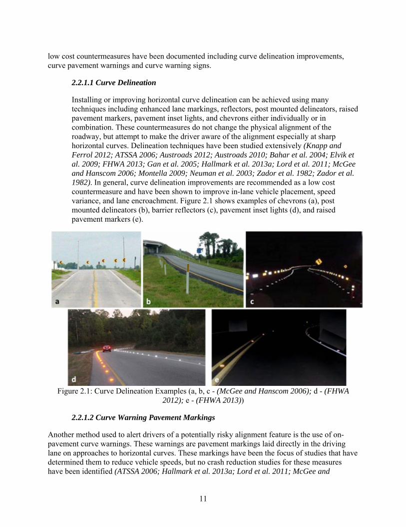
Installing or improving horizontal curve delineation can be achieved using many techniques including enhanced lane markings, reflectors, post mounted delineators, raised pavement markers, pavement inset lights, and chevrons either individually or in combination. These countermeasures do not change the physical alignment of the roadway, but attempt to make the driver aware of the alignment especially at sharp horizontal curves. Delineation techniques have been studied extensively (Knapp and Ferrol 2012; ATSSA 2006; Austroads 2012; Austroads 2010; Bahar et al. 2004; Elvik et al. 2009; FHWA 2013; Gan et al. 2005; Hallmark et al. 2013a; Lord et al. 2011; McGee and Hanscom 2006; Montella 2009; Neuman et al. 2003; Zador et al. 1982; Zador et al. 1982). In general, curve delineation improvements are recommended as a low cost countermeasure and have been shown to improve in-lane vehicle placement, speed variance, and lane encroachment. Figure 2.1 shows examples of chevrons (a), post mounted delineators (b), barrier reflectors (c), pavement inset lights (d), and raised pavement markers (e).

Figure 2.1: Curve Delineation Examples (a, b, c - (McGee and Hanscom 2006); d - (FHWA 2012); e - (FHWA 2013))

2.2.1.2 Curve Warning Pavement Markings

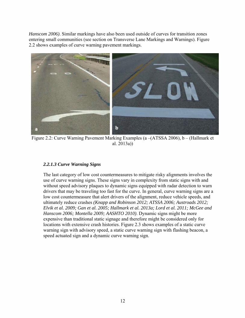
Another method used to alert drivers of a potentially risky alignment feature is the use of on-pavement curve warnings. These warnings are pavement markings laid directly in the driving lane on approaches to horizontal curves. These markings have been the focus of studies that have determined them to reduce vehicle speeds, but no crash reduction studies for these measures have been identified (ATSSA 2006; Hallmark et al. 2013a; Lord et al. 2011; McGee and

12

Hanscom 2006). Similar markings have also been used outside of curves for transition zones entering small communities (see section on Transverse Lane Markings and Warnings). Figure 2.2 shows examples of curve warning pavement markings.

Figure 2.2: Curve Warning Pavement Marking Examples (a –(ATSSA 2006), b – (Hallmark et al. 2013a))

2.2.1.3 Curve Warning Signs

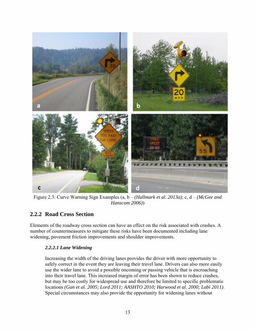
The last category of low cost countermeasures to mitigate risky alignments involves the use of curve warning signs. These signs vary in complexity from static signs with and without speed advisory plaques to dynamic signs equipped with radar detection to warn drivers that may be traveling too fast for the curve. In general, curve warning signs are a low cost countermeasure that alert drivers of the alignment, reduce vehicle speeds, and ultimately reduce crashes (Knapp and Robinson 2012; ATSSA 2006; Austroads 2012; Elvik et al. 2009; Gan et al. 2005; Hallmark et al. 2013a; Lord et al. 2011; McGee and Hanscom 2006; Montella 2009; AASHTO 2010). Dynamic signs might be more expensive than traditional static signage and therefore might be considered only for locations with extensive crash histories. Figure 2.3 shows examples of a static curve warning sign with advisory speed, a static curve warning sign with flashing beacon, a speed actuated sign and a dynamic curve warning sign.

13

Figure 2.3: Curve Warning Sign Examples (a, b – (Hallmark et al. 2013a); c, d – (McGee and Hanscom 2006))

2.2.2 Road Cross Section

Elements of the roadway cross section can have an effect on the risk associated with crashes. A number of countermeasures to mitigate these risks have been documented including lane widening, pavement friction improvements and shoulder improvements.

2.2.2.1 Lane Widening

Increasing the width of the driving lanes provides the driver with more opportunity to safely correct in the event they are leaving their travel lane. Drivers can also more easily use the wider lane to avoid a possible oncoming or passing vehicle that is encroaching into their travel lane. This increased margin of error has been shown to reduce crashes, but may be too costly for widespread use and therefore be limited to specific problematic locations (Gan et al. 2005; Lord 2011; AASHTO 2010; Harwood et al. 2000; Labi 2011). Special circumstances may also provide the opportunity for widening lanes without

14

adding pavement width by reducing shoulder width, if adequate shoulders exist at certain locations. A weighing of benefits of wider lanes and shoulder widths may be possible (see effectiveness of lane and shoulder widths in next section).

2.2.2.2 Pavement Friction

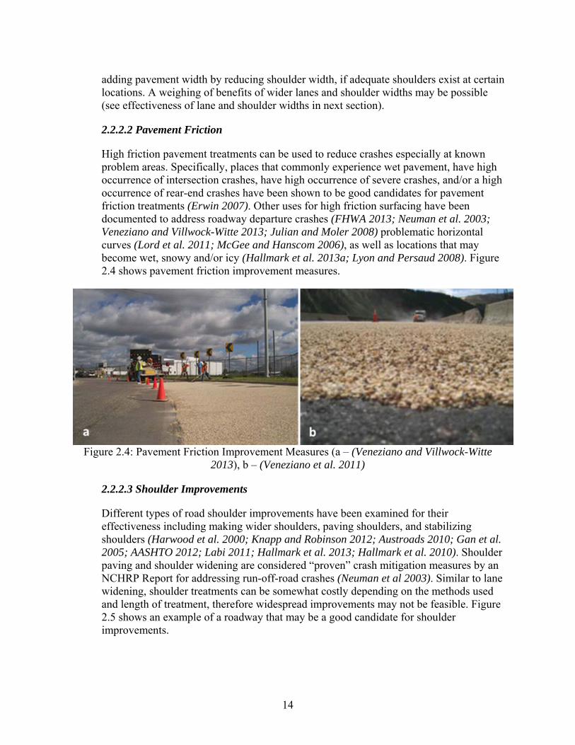
High friction pavement treatments can be used to reduce crashes especially at known problem areas. Specifically, places that commonly experience wet pavement, have high occurrence of intersection crashes, have high occurrence of severe crashes, and/or a high occurrence of rear-end crashes have been shown to be good candidates for pavement friction treatments (Erwin 2007). Other uses for high friction surfacing have been documented to address roadway departure crashes (FHWA 2013; Neuman et al. 2003; Veneziano and Villwock-Witte 2013; Julian and Moler 2008) problematic horizontal curves (Lord et al. 2011; McGee and Hanscom 2006), as well as locations that may become wet, snowy and/or icy (Hallmark et al. 2013a; Lyon and Persaud 2008). Figure 2.4 shows pavement friction improvement measures.

Figure 2.4: Pavement Friction Improvement Measures (a – (Veneziano and Villwock-Witte 2013), b – (Veneziano et al. 2011)

2.2.2.3 Shoulder Improvements

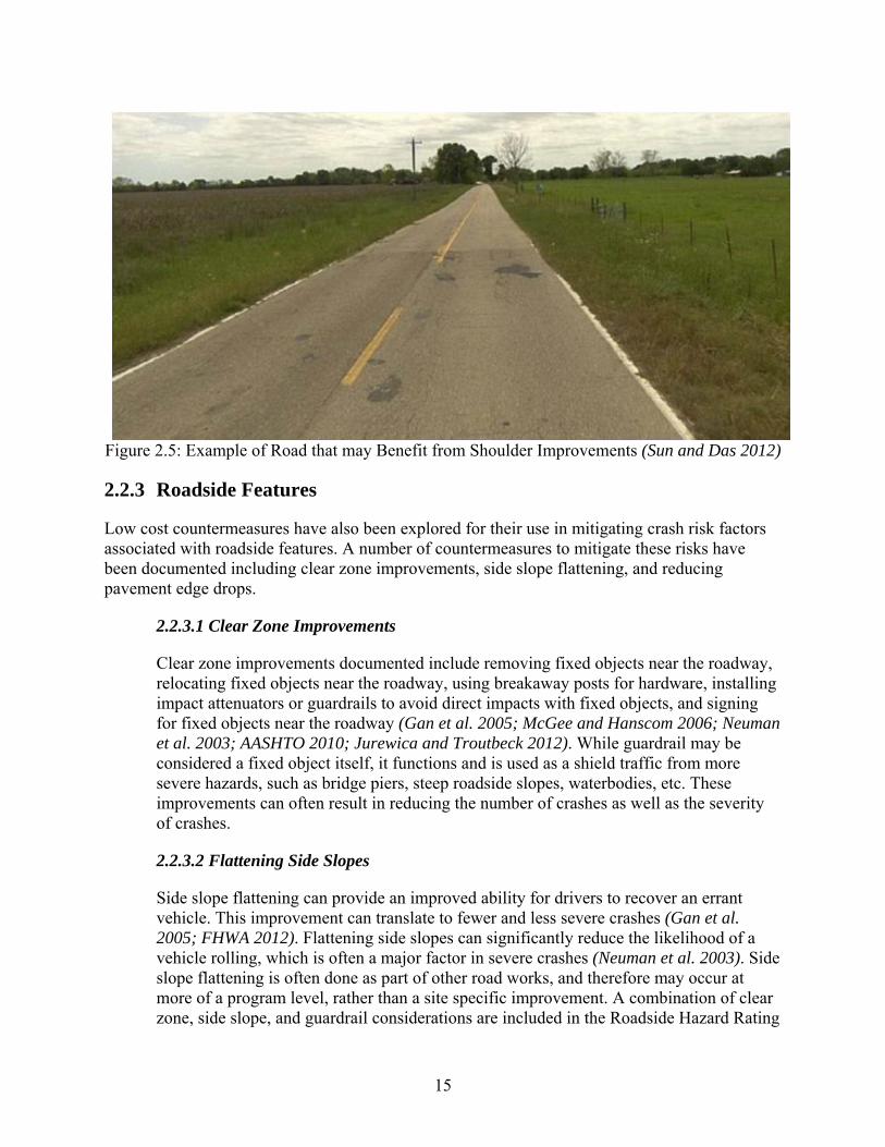
Different types of road shoulder improvements have been examined for their effectiveness including making wider shoulders, paving shoulders, and stabilizing shoulders (Harwood et al. 2000; Knapp and Robinson 2012; Austroads 2010; Gan et al. 2005; AASHTO 2012; Labi 2011; Hallmark et al. 2013; Hallmark et al. 2010). Shoulder paving and shoulder widening are considered “proven” crash mitigation measures by an NCHRP Report for addressing run-off-road crashes (Neuman et al 2003). Similar to lane widening, shoulder treatments can be somewhat costly depending on the methods used and length of treatment, therefore widespread improvements may not be feasible. Figure 2.5 shows an example of a roadway that may be a good candidate for shoulder improvements.

15

Figure 2.5: Example of Road that may Benefit from Shoulder Improvements (Sun and Das 2012)

2.2.3 Roadside Features

Low cost countermeasures have also been explored for their use in mitigating crash risk factors associated with roadside features. A number of countermeasures to mitigate these risks have been documented including clear zone improvements, side slope flattening, and reducing pavement edge drops.

2.2.3.1 Clear Zone Improvements

Clear zone improvements documented include removing fixed objects near the roadway, relocating fixed objects near the roadway, using breakaway posts for hardware, installing impact attenuators or guardrails to avoid direct impacts with fixed objects, and signing for fixed objects near the roadway (Gan et al. 2005; McGee and Hanscom 2006; Neuman et al. 2003; AASHTO 2010; Jurewica and Troutbeck 2012). While guardrail may be considered a fixed object itself, it functions and is used as a shield traffic from more severe hazards, such as bridge piers, steep roadside slopes, waterbodies, etc. These improvements can often result in reducing the number of crashes as well as the severity of crashes.

2.2.3.2 Flattening Side Slopes

Side slope flattening can provide an improved ability for drivers to recover an errant vehicle. This improvement can translate to fewer and less severe crashes (Gan et al. 2005; FHWA 2012). Flattening side slopes can significantly reduce the likelihood of a vehicle rolling, which is often a major factor in severe crashes (Neuman et al. 2003). Side slope flattening is often done as part of other road works, and therefore may occur at more of a program level, rather than a site specific improvement. A combination of clear zone, side slope, and guardrail considerations are included in the Roadside Hazard Rating

16

(RHR) system. The RHR for a roadway segment is a value from 1 (safest) to 7 (least safe) that describes the state of the clear zone, side slopes, and guardrail presence. Improvements in RHR have also been tied to quantifiable improvements in safety (AASHTO 2010).

2.2.3.3 Prevent Pavement Edge Drops

Pavement edge drops can develop from roadside erosion and/or pavement buildup from resurfacing projects. When these drops become too abrupt or too deep, crashes result from drivers’ inability to recover errant vehicles. Reducing pavement edge drops can be beneficial (Lord et al. 2011; Neuman et al. 2003; FHWA 2011; Hallmark et al. 2012) and is considered low cost especially when resurfacing is taking place as it may only require a modification to the existing surfacing equipment. Figure 5.6 shows a pavement edge drop.

Figure 2.6: Example of Pavement Edge Drop (Kirk 2008)

2.2.4 Other Measures

Many other low cost countermeasures that don’t fall in the previous three categories have been employed and experimented with in the documented literature. These countermeasures include centerline and edge line marking improvements, centerline and shoulder rumble strips and stripes, lighting improvements, other warning signs, transverse lane markings and warnings, and transverse rumble strips.

2.2.4.1 Centerline and Edge-line Marking Improvements

Installing, widening, and/or improving the reflectivity of edge lines and centerlines are improvements that have produced beneficial safety results (ATSSA 2006; Austroads

17

2010; Elvik et al. 2009; Gan et al. 2005; Lord et al. 2011; Neuman et al. 2003; Sun and Das 2012; Al-Masaeid and Sinha 1994; Donnell et al. 2009; Park et al. 2012; Potts et al. 2011). Pavement line markings provide valuable guidance for drivers especially at night. Typical line widths used are 4 inches, but wider markings up to 8 inches have been tried as well (Park et al. 2012). Enhanced line markings have also been used successfully as part of larger statewide safety improvement programs like the Missouri DOT Total Stripping and Delineation Program (Potts et al. 2011).

2.2.4.2 Centerline and Edge-line rumble Strips / Stripes

Rumble strips have been used and studied extensively in the documented literature. Centerline rumble strips are used on two lane undivided roadways to alter drivers encroaching into oncoming traffic. Shoulder rumble strips and edge line rumble stripes are used to alert drivers that may be leaving the roadway. Centerline and shoulder/edge line rumble strips have been used alone and in combination both on curves and tangent roadway sections to improve safety (ATSSA 2006; Lord et al. 2011; McGee and Hanscom 2006; Neuman et al. 2003; AASHTO 2010; Hallmark et al. 2010; Kirk 2008; Abdel-Rahim and Khan 2012; Datta et al. 2012; Hallmark et al. 2013; Monsere 2002; NCHRP 2005; Olson et al. 2013; Persaud et al. 2003). Both types of rumble strips/stripes have been shown to reduce crashes. Centerline rumble strips have also been shown to improve in-lane vehicle placement (Mahoney et al. 2003), and rumble stripes have also been shown to improve daytime and nighttime edge line visibility (Filcek et al. 2004). (See Figure 2.7)

Figure 2.7: Example of Centerline and Shoulder Rumble Strips (a – (Datta et al. 2012), b - WTI)

18

2.2.4.3 Lighting Improvements

The installation and enhancement of lighting has also been used to improve safety. The installation of lighting is typically targeted at intersections, but has also been envisioned for problematic horizontal curves (Austroads 2012; Gan 2005; Lord et al. 2011; AASHTO 2010; ITE 2007). Typically lighted intersections are mostly in urban and suburban areas, but lighting rural intersections may also have significant benefits (Isebrands et al. 2010).

2.2.4.4 Other Warning Signs

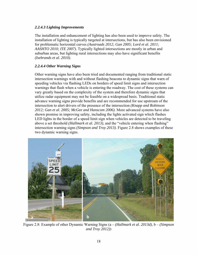
Other warning signs have also been tried and documented ranging from traditional static intersection warnings with and without flashing beacons to dynamic signs that warn of speeding vehicles via flashing LEDs on borders of speed limit signs and intersection warnings that flash when a vehicle is entering the roadway. The cost of these systems can vary greatly based on the complexity of the system and therefore dynamic signs that utilize radar equipment may not be feasible on a widespread basis. Traditional static advance warning signs provide benefits and are recommended for use upstream of the intersection to alert drivers of the presence of the intersection (Knapp and Robinson 2012; Gan et al. 2005; McGee and Hanscom 2006). More advanced systems have also shown promise in improving safety, including the lights activated sign which flashes LED lights in the border of a speed limit sign when vehicles are detected to be traveling above a set threshold (Hallmark et al. 2013), and the “vehicle entering when flashing” intersection warning signs (Simpson and Troy 2013). Figure 2.8 shows examples of these two dynamic warning signs.

B Figure 2.8: Example of other Dynamic Warning Signs (a – (Hallmark et al. 2013d), b – (Simpson

and Troy 2012))

19

2.2.4.5 Transverse Lane Markings and Warnings

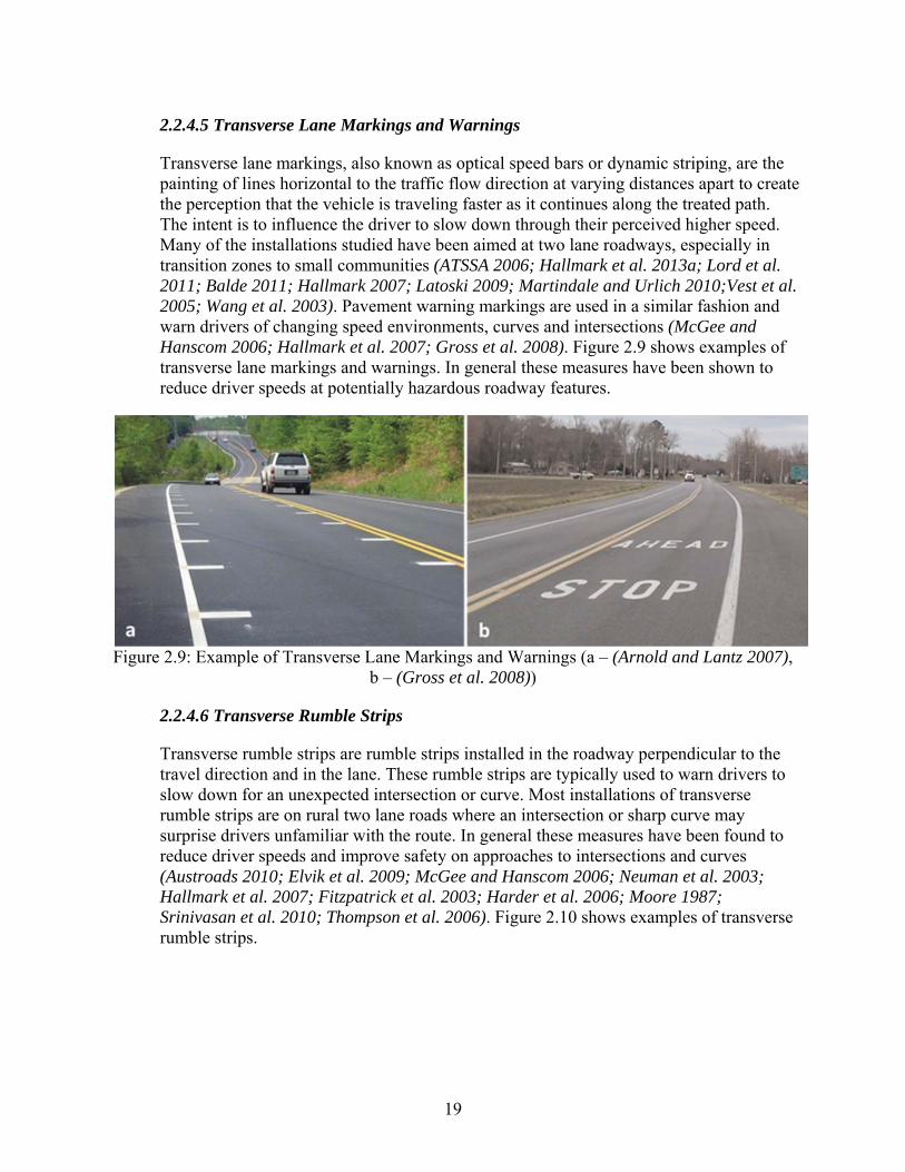
Transverse lane markings, also known as optical speed bars or dynamic striping, are the painting of lines horizontal to the traffic flow direction at varying distances apart to create the perception that the vehicle is traveling faster as it continues along the treated path. The intent is to influence the driver to slow down through their perceived higher speed. Many of the installations studied have been aimed at two lane roadways, especially in transition zones to small communities (ATSSA 2006; Hallmark et al. 2013a; Lord et al. 2011; Balde 2011; Hallmark 2007; Latoski 2009; Martindale and Urlich 2010;Vest et al. 2005; Wang et al. 2003). Pavement warning markings are used in a similar fashion and warn drivers of changing speed environments, curves and intersections (McGee and Hanscom 2006; Hallmark et al. 2007; Gross et al. 2008). Figure 2.9 shows examples of transverse lane markings and warnings. In general these measures have been shown to reduce driver speeds at potentially hazardous roadway features.

Figure 2.9: Example of Transverse Lane Markings and Warnings (a – (Arnold and Lantz 2007), b – (Gross et al. 2008))

2.2.4.6 Transverse Rumble Strips

Transverse rumble strips are rumble strips installed in the roadway perpendicular to the travel direction and in the lane. These rumble strips are typically used to warn drivers to slow down for an unexpected intersection or curve. Most installations of transverse rumble strips are on rural two lane roads where an intersection or sharp curve may surprise drivers unfamiliar with the route. In general these measures have been found to reduce driver speeds and improve safety on approaches to intersections and curves (Austroads 2010; Elvik et al. 2009; McGee and Hanscom 2006; Neuman et al. 2003; Hallmark et al. 2007; Fitzpatrick et al. 2003; Harder et al. 2006; Moore 1987; Srinivasan et al. 2010; Thompson et al. 2006). Figure 2.10 shows examples of transverse rumble strips.

20

Figure 2.10: Example of Transverse Rumble Strips (a – (Fitzpatrick et al. 2003), b – (Harder et al. 2006))

2.2.5 Countermeasure Effectiveness and Benefit/Cost

Many documented studies have evaluated the effectiveness of the previously identified low cost countermeasures. Crash reduction factors and crash modification factors are often reported and occasionally a benefit / cost analysis for the countermeasure is also included in the reporting. The effectiveness values cited in this section are focused on those that may best represent lower volume roads.

2.2.5.1 Alignment Countermeasures Effectiveness

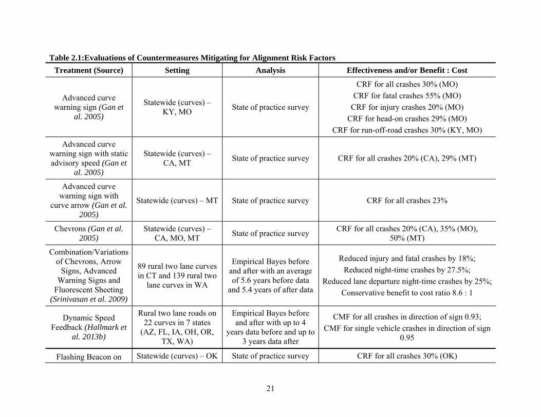
Table 2.1 provides the results from evaluations of countermeasures mitigating for alignment risk factors.

21

Table 2.1:Evaluations of Countermeasures Mitigating for Alignment Risk Factors

Treatment (Source) Setting Analysis Effectiveness and/or Benefit : Cost

Advanced curve warning sign (Gan et

al. 2005)

Statewide (curves) – KY, MO

State of practice survey

CRF for all crashes 30% (MO)

CRF for fatal crashes 55% (MO)

CRF for injury crashes 20% (MO)

CRF for head-on crashes 29% (MO)

CRF for run-off-road crashes 30% (KY, MO)

Advanced curve warning sign with static advisory speed (Gan et

al. 2005)

Statewide (curves) – CA, MT

State of practice survey CRF for all crashes 20% (CA), 29% (MT)

Advanced curve warning sign with

curve arrow (Gan et al. 2005)

Statewide (curves) – MT State of practice survey CRF for all crashes 23%

Chevrons (Gan et al. 2005)

Statewide (curves) – CA, MO, MT

State of practice survey CRF for all crashes 20% (CA), 35% (MO),

50% (MT)

Combination/Variations of Chevrons, Arrow

Signs, Advanced Warning Signs and

Fluorescent Sheeting (Srinivasan et al. 2009)

89 rural two lane curves in CT and 139 rural two

lane curves in WA

Empirical Bayes before and after with an average of 5.6 years before data

and 5.4 years of after data

Reduced injury and fatal crashes by 18%;

Reduced night-time crashes by 27.5%;

Reduced lane departure night-time crashes by 25%;

Conservative benefit to cost ratio 8.6 : 1

Dynamic Speed Feedback (Hallmark et

al. 2013b)

Rural two lane roads on 22 curves in 7 states

(AZ, FL, IA, OH, OR, TX, WA)

Empirical Bayes before and after with up to 4

years data before and up to 3 years data after

CMF for all crashes in direction of sign 0.93;

CMF for single vehicle crashes in direction of sign 0.95

Flashing Beacon on Statewide (curves) – OK State of practice survey CRF for all crashes 30% (OK)

22

Curve Warning (Gan et al. 2005)

Install horizontal alignment and advisory speed signs (AASHTO

2010)

Unspecified Combination of studies CMF for injury crashes 0.87*

CMF for non-injury crashes 0.71*

Post Mounted Delineators (McGee and Hanscom 2006)

Rural two lane curves in OH

Unknown Reduced run-off-road crashes by 15%

Post mounted delineators (Gan et al.

2005)

Statewide (curves) – AK, MO, MT

State of practice survey CRF for all crashes 20% (AK), 25% (MO),

30% (MT)

Raised Pavement Markers (FHWA 2013)

10 rural roadways (tangents and curves) in Mobile County, AL with

documented high run-off-road crashes

Simple before and after with 4 years data before

and 4 years data after

Total crashes reduced from 224 to 33;

Fatalities from 7 to 0;

Injuries from 152 to 10

23

Raised Pavement Markers (Gan et al.

2005)

Statewide (tangents and curves) – AZ, IN, KY,

MO, OK, VT State of practice survey

CRF for total crashes 4% (IN), 10% (MO), 11% (AZ), 16% (VT);

CRF for head on crashes 12% (AZ), 20% (MO);

CRF for side-swipe crashes 13% (AZ), 20% (MO);

CRF for fixed object crashes 10% (MO);

CRF for run-off-road crashes 10% (MO), 33% (AZ);

CRF for wet pavement crashes 25% (KY, MO);

CRF for nighttime crashes 16% (AZ), 20% (KY, MO), 30% (OK)

Raised Pavement Markers (Zadot et al.

1982)

662 two lane horizontal curves in GA with

curvature > 6 degrees

Before and after with statistical testing

Reduction in nighttime crashes of 22%;

Raised Pavement Markers (Neuman et

al. 2003)

184 high accident locations (including

curves, narrow bridges, and intersection

approaches)

Before and after with 1 year before and 1 year after

data

Reduced all accidents by 9%;

Reduced injuries by 15%;

Benefit to cost ratio of 6.5 : 1

Raised Pavement Markers (Neuman et

al. 2003)

8 rural two lane roads in NJ, selected for high

crash history

Before and after with 2 years before and 1 year

after data

Unspecified reduction in crashes resulting in benefit to cost ratios ranging from 15.5 : 1 to 25.5 : 1

* Indicates CMF (or equivalent CMF based on CRF) is reported in the Highway Safety Manual (HSM).

24

2.2.5.2 Road Cross-Section Countermeasures Effectiveness

Table 2.2 provides the results from evaluations of countermeasures mitigating for road cross-section related risk factors.

Table 2.2: Evaluations of Countermeasures Mitigating for Road Cross-Section Related Risk Factors


Adding Paved Shoulders (Hallmark

et al. 2013c)

220 road segments (both 2-lane and 4-lane) in

Iowa

Before-and-after with comparison to expected

crashes with control sections and generalized

linear models

CRF for total crashes 4%, and CRF for run-off-road crashes 8%

per every additional foot of shoulder added.

Change Shoulders from Turf to

Pavement

(Harwood et al. 2000; AASHTO 2010)

Rural two lane roads

Combine approach using historical crash data,

regression analysis, before-and-after studies, and

expert judgment

CFRs for run-off-road, side-swipe, and opposite direction crashes:

for 1ft shoulder: 1%*






High Friction Overlay (Veneziano and

Villwock-Witte 2013)

Rural two lane highway segment with high crash

history – PA.

Simple before and after with 9 years before data and 1 year of after data.

Total crashes reduced from 22 in before period to 0 in the after period (limited timeframe reported).

High Friction Surface Treatment (FHWA

2013)

75 targeted rural two lane roads – KY

Simple before and after with 3 years before and 3

years after data

Wet-weather roadway departure crashes reduced from 357 to 33;

Dry-weather roadway departure crashes reduced from 126 to 28

25

Increase pavement friction number - 5 unit increase (Labi

2011)

540 rural two lane road segments in IN

(effectiveness for rural major collectors shown):

empirical analysis using negative binomial

modeling technique

CRF for fatal and injury crashes 8%;

CRF for injury crashes 8%;

CRF for PDO crashes 9%

Pave Shoulder (Gan et al. 2005)

Statewide – KY, MO State of practice survey CRF for total crashes 15% (KY, MO)

Pave Shoulder (Austroads 2010)

Statewide – Australia Meta-analysis CRF for total crashes 30%

Resurface with skid resistant pavement (Gan et al. 2005)

Statewide (curves) – CA, MO, MT


CRF for all crashes 10% (CA), 24% (MT);

CRF for head-on crashes 86% (MO);

CRF for wet pavement crashes 51% (MO)

Resurface with skid resistant pavement (Gan et al. 2005)

Statewide – IN, NY State of practice survey

CRF for all crashes 7% (IN), 8% (NY);

CRF for right-angle crashes 31% (NY);

CRF for wet pavement crashes 35% (NY)

Skid Resistant Improvements (Lyon and Persaud 2008)

Rural two lane road segments identified as high wet-road crash

locations and having low friction numbers – NY.

Empirical Bayes before and after with an average of 5 years before data and

4 years of after data

CRF for all crashes 4%;

CRF for wet-road crashes 15%;

Rear-end and dry-road crashes showed slight increases in crashes after treatment.

(These values were not found to be statistically significant at the 5% level.)

Skid Resistant Improvements with curve warning sign

(McGee and Hanscom 2006)

Rural two lane curve Simple before and after

with 13 months before and 6 months after

Wet-pavement crashes reduced from 16 in before period to two in after period.

26

Skid treatment with overlay (Gan et al.

2005) Statewide – MN, NY State of practice survey

CRF for all crashes 13% (NY);

CRF for head-on crashes 19% (MN fatal+inj), 30% (MN pdo), 43% (NY);

CRF for rear-end crashes 12% (MN fatal+inj), 21% (MN pdo);

CRF for right-angle crashes 11% (MN fatal+inj), 23% (NY), 31%(MN pdo);

CRF for side-swipe crashes 12% (MN fatal+inj), 27% (MN pdo), 43% (NY);

CRF for left-turn crashes 34% (MN pdo), 41% (MN fatal+inj);

CRF for fixed-object crashes 43% (NY);

CRF for pedestrian crashes 3% (MN fatal+inj);

CRF for run-off-road crashes 28% (MN fatal+inj), 29% (MN pdo);

CRF for wet pavement crashes 23% (NY)

Stabilize Shoulder (Gan et al. 2005)

Statewide – KY, MO State of practice survey CRF for total crashes 25%, (KY, MO)

Widen Lanes


Rural two lane highways with ADT < 400 vpd



expert judgment


9ft to 10ft: 3%*

9ft to 11ft: 4%*

9ft to 12ft: 5%*

Widen Lanes


Rural two lane highways with ADT approximately

1000 vpd



expert judgment


9ft to 10ft: 10%*

9ft to 11ft: 18%*

9ft to 12ft: 20%*

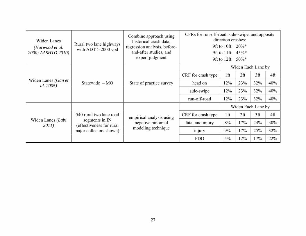
27

Widen Lanes


Rural two lane highways with ADT > 2000 vpd



expert judgment


9ft to 10ft: 20%*

9ft to 11ft: 45%*

9ft to 12ft: 50%*

Widen Lanes (Gan et al. 2005)

Statewide – MO State of practice survey

Widen Each Lane by

CRF for crash type 1ft 2ft 3ft 4ft

head on 12% 23% 32% 40%

side-swipe 12% 23% 32% 40%

run-off-road 12% 23% 32% 40%

Widen Lanes (Labi 2011)




modeling technique

Widen Each Lane by


fatal and injury 8% 17% 24% 30%

injury 9% 17% 25% 32%

PDO 5% 12% 17% 22%

28

Widen Paved Shoulder (Gan et al.

2005) Statewide – MO State of practice survey

Widen Each Shoulder by


fixed-object 16% 29% 40% 49%

run-off-road 16% 29% 40% 49%

Widen Paved Shoulder by

unspecified amount (Gan et al. 2005)

Statewide – AZ, CA, IA, MI, MT, VA


CRF for total crashes 8% (IA), 20% (CA), 32% (MT), 57% (AZ);

CRF for fatal crashes 50% (VA);

CRF for injury crashes 50% (VA);

CRF for PDO crashes 50% (VA);

CRF for head-on crashes 15% (MI), 75% (AZ);

CRF for side-swipe crashes 15% (MI), 41% (AZ);

CRF for fixed-object crashes 15% (MI);

CRF for pedestrian crashes 71% (AZ);

CRF for run-off-road crashes 60% (AZ)

Widen Shoulder by 1 foot each (Labi 2011)




modeling technique

% reduction shown Widen Each Shoulder by

CRF for crash type 1ft 2ft 3ft 4ft 5ft 6ft

fatal and injury 4 5 9 12 15 18

injury 4 5 9 11 14 16

PDO 1 2 4 5 6 7

29

Widen Shoulders


Rural two lane highways with < 400 ADT



expert judgment


0ft to 2ft: 4%*

0ft to 4ft: 9%*

0ft to 6ft: 12%*

0ft to 8ft: 15%*

Widen Shoulders


Rural two lane highways with ADT approximately

1000 vpd



expert judgment


0ft to 2ft: 8%*

0ft to 4ft: 18%*

0ft to 6ft: 24%*

0ft to 8ft: 30%*

Widen Shoulders


Rural two lane highways with > 2000 ADT



expert judgment


0ft to 2ft: 20%*

0ft to 4ft: 35%*

0ft to 6ft: 50%*

0ft to 8ft: 63%*

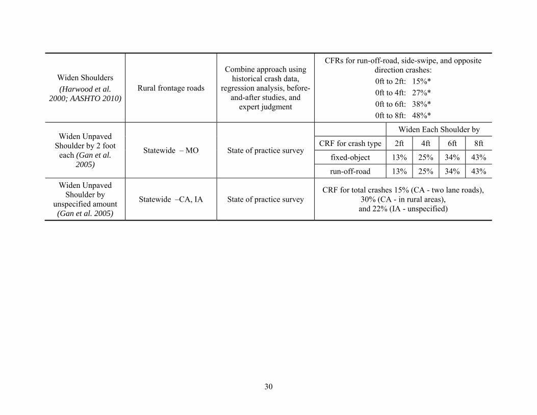
30

Widen Shoulders


Rural frontage roads



expert judgment


0ft to 2ft: 15%*

0ft to 4ft: 27%*

0ft to 6ft: 38%*

0ft to 8ft: 48%*

Widen Unpaved Shoulder by 2 foot

each (Gan et al. 2005)


Widen Each Shoulder by


fixed-object 13% 25% 34% 43%

run-off-road 13% 25% 34% 43%

Widen Unpaved Shoulder by

unspecified amount (Gan et al. 2005)

Statewide –CA, IA State of practice survey CRF for total crashes 15% (CA - two lane roads),

30% (CA - in rural areas), and 22% (IA - unspecified)

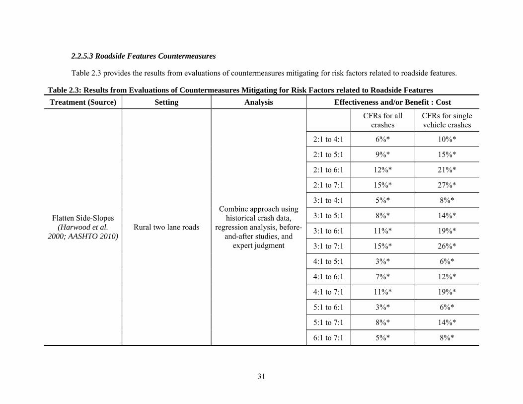
31

2.2.5.3 Roadside Features Countermeasures

Table 2.3 provides the results from evaluations of countermeasures mitigating for risk factors related to roadside features.

Table 2.3: Results from Evaluations of Countermeasures Mitigating for Risk Factors related to Roadside Features


Flatten Side-Slopes (Harwood et al.

2000; AASHTO 2010) Rural two lane roads



expert judgment

CFRs for all

crashes CFRs for single vehicle crashes

2:1 to 4:1 6%* 10%*

2:1 to 5:1 9%* 15%*

2:1 to 6:1 12%* 21%*

2:1 to 7:1 15%* 27%*

3:1 to 4:1 5%* 8%*

3:1 to 5:1 8%* 14%*

3:1 to 6:1 11%* 19%*

3:1 to 7:1 15%* 26%*

4:1 to 5:1 3%* 6%*

4:1 to 6:1 7%* 12%*

4:1 to 7:1 11%* 19%*

5:1 to 6:1 3%* 6%*

5:1 to 7:1 8%* 14%*

6:1 to 7:1 5%* 8%*

32

Flatten Side-Slopes in General (Gan et al.

2005)

Statewide – AZ, IA, KY, MT, NY, OK


CRF for total crashes 25% (IA), 30% (KY, OK), 32% (MT), 43% (NY);



Flatten Side-Slopes in General (Neuman et

al. 2003)

All roads with grade improvements

completed 1986 – 1991 in WA

Before and after with statistical significance

testing

CRF for total crashes 3% to 50%;

Median CRF for run-off-road crashes 25% to 45%

Improve Roadside Hazard Rating

(AASHTO 2010) Rural two lane roads Not Specified

CMF for total crashes

RHR 7 to 6: 0.94*

RHR 7 to 5: 0.87*

RHR 7 to 4: 0.82*

RHR 7 to 3: 0.77*

RHR 7 to 2: 0.72*

RHR 7 to 1: 0.67*

Increase Clear Zone (AASHTO 2010)

Rural two lane roads Combination of studies

CMF for total crashes

increase clear zone 3.3ft to 16.7ft: 0.78*

increase clear zone 16.7ft to 30.0ft: 0.56*

Increase Clear Zone (Gan et al. 2005)


CFRs for fixed object and run-off-road crashes:

increase clear zone 5ft: 13%





Install Object Markers (Gan et al. 2005)

Statewide – AZ, MO State of practice survey

CRF for total crashes 16% (AZ, MO);

CRF for fatal crashes 41% (MO);

CRF for injury crashes 17% (MO);

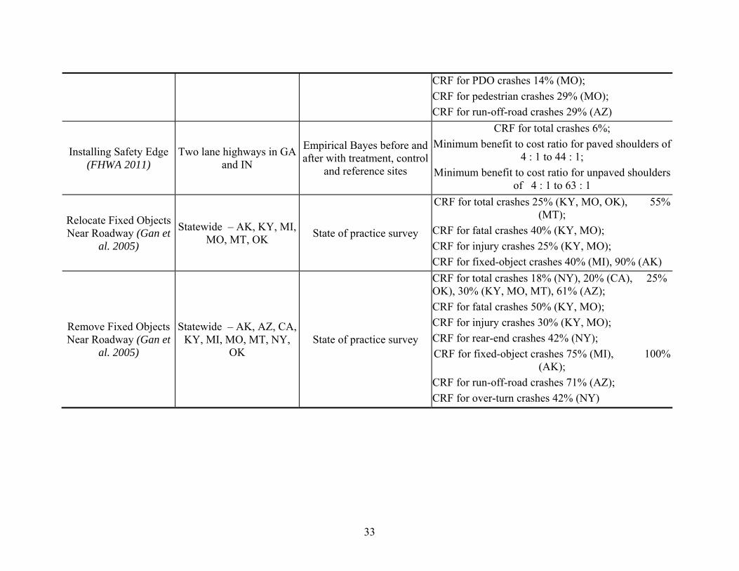
33

CRF for PDO crashes 14% (MO);

CRF for pedestrian crashes 29% (MO);


Installing Safety Edge (FHWA 2011)

Two lane highways in GA and IN

Empirical Bayes before and after with treatment, control

and reference sites

CRF for total crashes 6%;

Minimum benefit to cost ratio for paved shoulders of 4 : 1 to 44 : 1;

Minimum benefit to cost ratio for unpaved shoulders of 4 : 1 to 63 : 1

Relocate Fixed Objects Near Roadway (Gan et

al. 2005)

Statewide – AK, KY, MI, MO, MT, OK


CRF for total crashes 25% (KY, MO, OK), 55% (MT);

CRF for fatal crashes 40% (KY, MO);

CRF for injury crashes 25% (KY, MO);

CRF for fixed-object crashes 40% (MI), 90% (AK)

Remove Fixed Objects Near Roadway (Gan et

al. 2005)

Statewide – AK, AZ, CA, KY, MI, MO, MT, NY,

OK State of practice survey

CRF for total crashes 18% (NY), 20% (CA), 25% OK), 30% (KY, MO, MT), 61% (AZ);

CRF for fatal crashes 50% (KY, MO);

CRF for injury crashes 30% (KY, MO);

CRF for rear-end crashes 42% (NY);

CRF for fixed-object crashes 75% (MI), 100% (AK);

CRF for run-off-road crashes 71% (AZ);

CRF for over-turn crashes 42% (NY)

34

2.2.5.4 Other Countermeasures Effectiveness

Table 2.4 provides the results from evaluations of countermeasures mitigating for risk factors related to other features not included in the previous sections.

Table 2.4: Results from Evaluations of Countermeasures Mitigating for Risk Factors related to Other Features Not Included in the Previous Sections.


Install Centerline and Shoulder Rumble

Strips (Olson et al. 2013)

Rural two lane roads in WA

Before and after with 8 years of crash data total

CRF for lane departure crashes 66%

CRF for cross-over crashes 71%

CRF for run-off-the road (right) crashes 62%

Install Centerline Markings (Gan et al.

2005)

Statewide – KY, MO, OK

State of practice survey CRF for total crashes 30% (OK), 35% (KY, MO);

Install Centerline Rumble Strips

(AASHTO 2010; Persaud 2003)

210 miles of rural two lane roads in CA, CO,

DE, MD, MN, OR, WA


3 years after data

CRF for all crashes 14%*

CRF for opposite direction crashes 21%*

CRF for night time crashes 19%*;

CRF for day time crashes 9%*

Install Edge Line Markings (Sun and

Das 2012)

Narrow (pavement less than 22ft) rural two lane

highways in LA

Before and after with 3 years before data and 1

year after data and using control sites and statistical

testing

CMF for total crashes 0.78

35

Install Edge Line Markings (Gan et al.

2005)

Statewide – AZ, IA, KY, MO, NY, OK, TX


CRF for total crashes 4% (IA), 15% (KY, MO, OK), 25% (TX), 30% (AZ),

44% (NY);





CRF for run-off-road crashes 30% (AZ, KY, MO);

CRF for overturn crashes 45% (NY)

Install Flashing Beacon at or in

Advance of Intersection (Gan et

al. 2005)

Statewide – KY, MO, MT, OK

State of practice survey CRF for total crashes 25% (KY, MO, OK),

27% (MT), 30% (OK, MO)

Install Lighting (Isebrands et al.

2010)

33 isolated rural intersections in MN

Before and after with 3 years of before data and 3

years of after data with statistical testing

CRF for night crashes 37%

Install Lighting (AASHTO 2010)

All road types Combination of studies

CMF for nighttime crashes 0.80*

CMF for nighttime injury crashes 0.72*

CMF for nighttime non-injury crashes 0.83*

Install Lighting at Intersections (ITE

2007)

FHWA / ITE toolbox value for non-signalized

intersections Not Specified CRF for total crashes 47%

Install or Improve Street Lighting at

Intersections (Gan et al. 2005)

Statewide – AK, CA, KY, MO, MT, OK

State of practice survey CRF for total crashes 30% (KY, MO), 36% (CA);

CRF for night time crashes 50% (AK, KY, MO, OK), 64% (MT), 67% (CA)

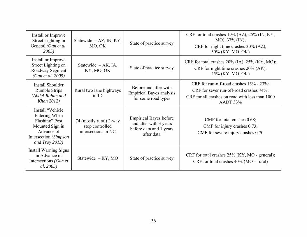
36

Install or Improve Street Lighting in

General (Gan et al. 2005)

Statewide – AZ, IN, KY, MO, OK


CRF for total crashes 19% (AZ), 25% (IN, KY, MO), 37% (IN);

CRF for night time crashes 30% (AZ), 50% (KY, MO, OK)

Install or Improve Street Lighting on Roadway Segment (Gan et al. 2005)

Statewide – AK, IA, KY, MO, OK

State of practice survey CRF for total crashes 20% (IA), 25% (KY, MO);

CRF for night time crashes 20% (AK), 45% (KY, MO, OK)

Install Shoulder Rumble Strips

(Abdel-Rahim and Khan 2012)

Rural two lane highways in ID

Before and after with Empirical Bayes analysis

for some road types

CRF for run-off-road crashes 15% - 23%;

CRF for sever run-off-road crashes 74%;

CRF for all crashes on road with less than 1000 AADT 33%

Install “Vehicle Entering When Flashing” Post

Mounted Sign in Advance of

Intersection (Simpson and Troy 2013)

74 (mostly rural) 2-way stop controlled

intersections in NC

Empirical Bayes before and after with 3 years

before data and 1 years after data

CMF for total crashes 0.68;

CMF for injury crashes 0.73;

CMF for severe injury crashes 0.70

Install Warning Signs in Advance of


Statewide – KY, MO State of practice survey CRF for total crashes 25% (KY, MO - general);

CRF for total crashes 40% (MO – rural)

37

Pavement Marking Improvements (Al-Masaeid and Sinha

1994)

Hazardous two lane rural road segments in IN

Empirical Bayes before and after

CRF for total crashes 14%

“Stop Ahead” Pavement Warning (Gross et al. 2008)

175 intersections in AR, MD, MN

Empirical Bayes before and after with more than 7 years before data and 2 years after

data

CRF for total crashes at 3-legged int. 60%


Transverse Rumble Strips (Moore 1987)

26 approaches to rural, low-volume, two lane, stop controlled intersections in LA selected for high crash

history

Before and after analysis with 2 years before and 2

years after data CRF for all crashes 29%

Transverse Rumble Strips (Srinivasan et al.

2010)

154 approaches to rural two way stop controlled

intersections in IA and MN

Empirical Bayes before and after with an average of 13

years before data and 6 years after data

CRF for evident injury or worse crashes 21%

CRF for incapacitating injury or worse crashes 39%

CRF for PDO crashes -19%

Overall economic crash harm reduction of $6,600 per year per intersection

Wider Edge Line Markings (Park et al.

2012)

Rural two lane highways in IL, KS, MI

Multiple approaches including Empirical Bayes

before and after and observational analysis

CRF for total crashes 18%, 19%, 27%, 30%;

CRF for fatal and injury crashes 15%, 16%, 37%, 38%;

CRF for PDO crashes 12%, 20%, 24%, 31%;

CRF for night crashes 4%, 19%, 30%, 31%;

CRF for wet crashes 23%, 35%, 63%, 67%;

CRF for fixed-object crashes 19%, 30%

Wider Marking on Centerline and Edge

Line (Potts et al. 2011)

Statewide stripping improvements on two lane

rural roadways in MI

Before and after with 3 years before data and 3 year after data and statistical testing

CFR for fatal and injury crashes 38%

Benefit cost ratio (for all road types) 11 : 1

38


Install Centerline and Shoulder Rumble

Strips (Olson et al. 2013)

Rural two lane roads in WA

Before and after with 8 years of crash data total

CRF for lane departure crashes 66%

CRF for cross-over crashes 71%

CRF for run-off-the road (right) crashes 62%

Install Centerline Markings (Gan et al.

2005)

Statewide – KY, MO, OK

State of practice survey CRF for total crashes 30% (OK), 35% (KY, MO);


(AASHTO 2010; Persaud 2003)

210 miles of rural two lane roads in CA, CO,

DE, MD, MN, OR, WA


3 years after data

CRF for all crashes 14%*

CRF for opposite direction crashes 21%*

CRF for night time crashes 19%*;

CRF for day time crashes 9%*

Install Edge Line Markings (Sun and

Das 2012)

Narrow (pavement less than 22ft) rural two lane

highways in LA

Before and after with 3 years before data and 1

year after data and using control sites and statistical

testing

CMF for total crashes 0.78

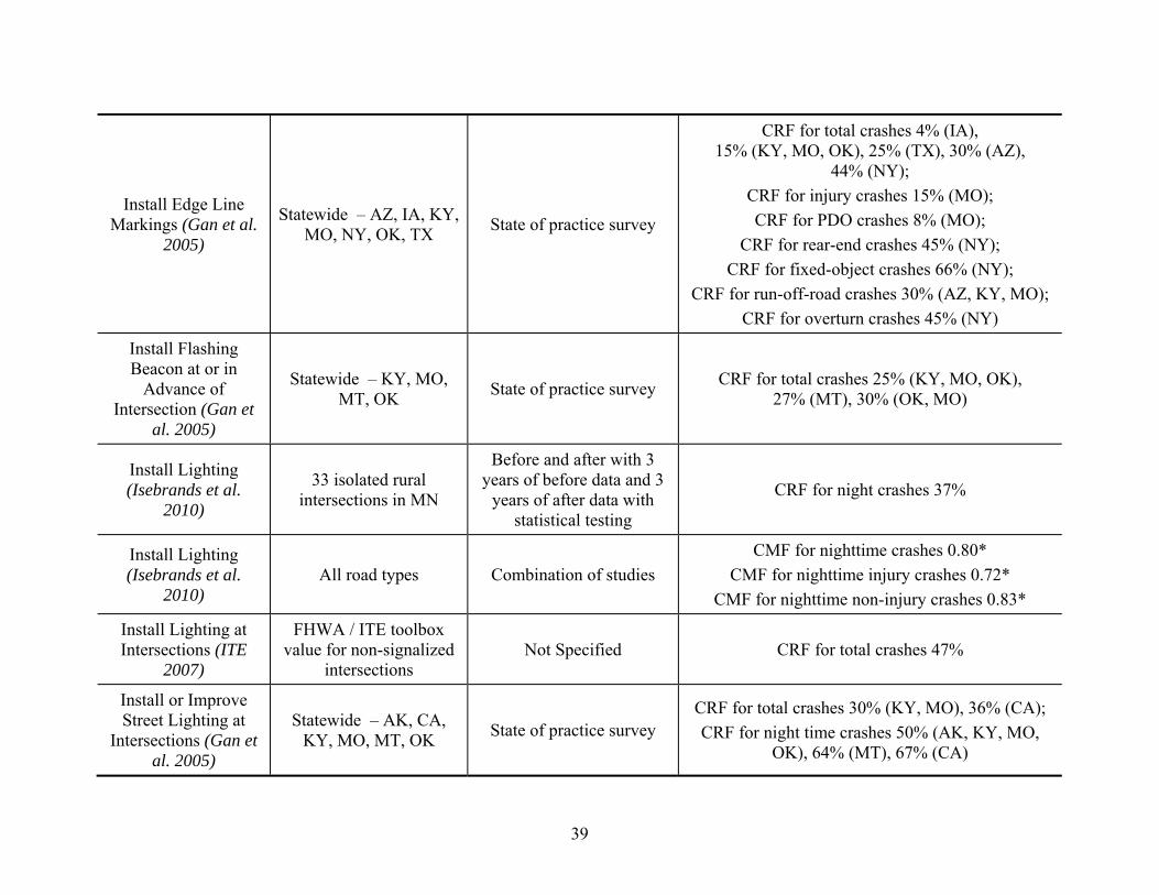
39

Install Edge Line Markings (Gan et al.

2005)

Statewide – AZ, IA, KY, MO, NY, OK, TX


CRF for total crashes 4% (IA), 15% (KY, MO, OK), 25% (TX), 30% (AZ),

44% (NY);





CRF for run-off-road crashes 30% (AZ, KY, MO);

CRF for overturn crashes 45% (NY)

Install Flashing Beacon at or in

Advance of Intersection (Gan et

al. 2005)

Statewide – KY, MO, MT, OK

State of practice survey CRF for total crashes 25% (KY, MO, OK),

27% (MT), 30% (OK, MO)


2010)

33 isolated rural intersections in MN

Before and after with 3 years of before data and 3

years of after data with statistical testing

CRF for night crashes 37%


2010) All road types Combination of studies

CMF for nighttime crashes 0.80*

CMF for nighttime injury crashes 0.72*

CMF for nighttime non-injury crashes 0.83*

Install Lighting at Intersections (ITE

2007)

FHWA / ITE toolbox value for non-signalized

intersections Not Specified CRF for total crashes 47%

Install or Improve Street Lighting at


Statewide – AK, CA, KY, MO, MT, OK

State of practice survey CRF for total crashes 30% (KY, MO), 36% (CA);

CRF for night time crashes 50% (AK, KY, MO, OK), 64% (MT), 67% (CA)

40

Install or Improve Street Lighting in

General (Gan et al. 2005)

Statewide – AZ, IN, KY, MO, OK


CRF for total crashes 19% (AZ), 25% (IN, KY, MO), 37% (IN);

CRF for night time crashes 30% (AZ), 50% (KY, MO, OK)

Install or Improve Street Lighting on Roadway Segment (Gan et al. 2005)

Statewide – AK, IA, KY, MO, OK

State of practice survey CRF for total crashes 20% (IA), 25% (KY, MO);

CRF for night time crashes 20% (AK), 45% (KY, MO, OK)

Install Shoulder Rumble Strips (ITE

2007)

Rural two lane highways in ID

Before and after with Empirical Bayes analysis

for some road types

CRF for run-off-road crashes 15% - 23%;

CRF for sever run-off-road crashes 74%;

CRF for all crashes on road with less than 1000 AADT 33%

Install “Vehicle Entering When Flashing” Post

Mounted Sign in Advance of

Intersection (ITE 2007)

74 (mostly rural) 2-way stop controlled

intersections in NC

Empirical Bayes before and after with 3 years

before data and 1 years after data

CMF for total crashes 0.68;

CMF for injury crashes 0.73;

CMF for severe injury crashes 0.70

Install Warning Signs in Advance of


Statewide – KY, MO State of practice survey CRF for total crashes 25% (KY, MO - general);

CRF for total crashes 40% (MO – rural)

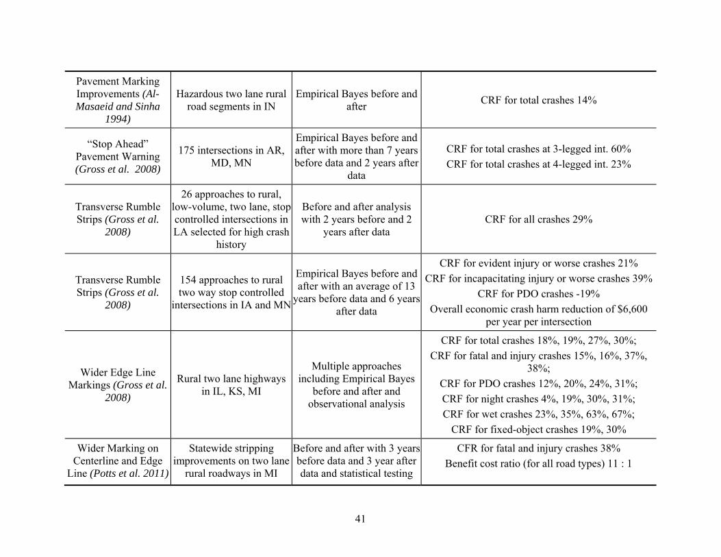
41

Pavement Marking Improvements (Al-Masaeid and Sinha

1994)

Hazardous two lane rural road segments in IN

Empirical Bayes before and after

CRF for total crashes 14%

“Stop Ahead” Pavement Warning (Gross et al. 2008)

175 intersections in AR, MD, MN

Empirical Bayes before and after with more than 7 years before data and 2 years after

data



Transverse Rumble Strips (Gross et al.

2008)

26 approaches to rural, low-volume, two lane, stop controlled intersections in LA selected for high crash

history

Before and after analysis with 2 years before and 2

years after data CRF for all crashes 29%

Transverse Rumble Strips (Gross et al.

2008)

154 approaches to rural two way stop controlled

intersections in IA and MN

Empirical Bayes before and after with an average of 13

years before data and 6 years after data

CRF for evident injury or worse crashes 21%

CRF for incapacitating injury or worse crashes 39%

CRF for PDO crashes -19%

Overall economic crash harm reduction of $6,600 per year per intersection

Wider Edge Line Markings (Gross et al.

2008)

Rural two lane highways in IL, KS, MI

Multiple approaches including Empirical Bayes

before and after and observational analysis

CRF for total crashes 18%, 19%, 27%, 30%;

CRF for fatal and injury crashes 15%, 16%, 37%, 38%;

CRF for PDO crashes 12%, 20%, 24%, 31%;

CRF for night crashes 4%, 19%, 30%, 31%;

CRF for wet crashes 23%, 35%, 63%, 67%;

CRF for fixed-object crashes 19%, 30%

Wider Marking on Centerline and Edge

Line (Potts et al. 2011)

Statewide stripping improvements on two lane

rural roadways in MI

Before and after with 3 years before data and 3 year after data and statistical testing

CFR for fatal and injury crashes 38%

Benefit cost ratio (for all road types) 11 : 1

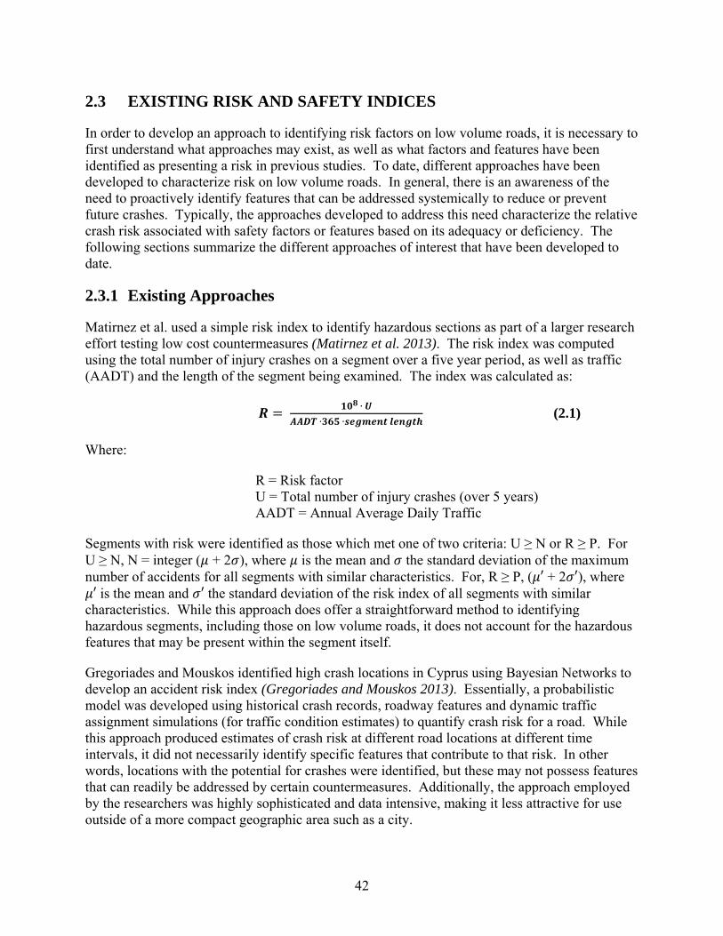
42

2.3 EXISTING RISK AND SAFETY INDICES

In order to develop an approach to identifying risk factors on low volume roads, it is necessary to first understand what approaches may exist, as well as what factors and features have been identified as presenting a risk in previous studies. To date, different approaches have been developed to characterize risk on low volume roads. In general, there is an awareness of the need to proactively identify features that can be addressed systemically to reduce or prevent future crashes. Typically, the approaches developed to address this need characterize the relative crash risk associated with safety factors or features based on its adequacy or deficiency. The following sections summarize the different approaches of interest that have been developed to date.

2.3.1 Existing Approaches

Matirnez et al. used a simple risk index to identify hazardous sections as part of a larger research effort testing low cost countermeasures (Matirnez et al. 2013). The risk index was computed using the total number of injury crashes on a segment over a five year period, as well as traffic (AADT) and the length of the segment being examined. The index was calculated as:

∙

∙ ∙ (2.1)

Where:

R = Risk factor U = Total number of injury crashes (over 5 years) AADT = Annual Average Daily Traffic

Segments with risk were identified as those which met one of two criteria: U ≥ N or R ≥ P. For U ≥ N, N = integer ( + 2 ), where is the mean and the standard deviation of the maximum number of accidents for all segments with similar characteristics. For, R ≥ P, ( ′ + 2 ′), where ′ is the mean and ′ the standard deviation of the risk index of all segments with similar

characteristics. While this approach does offer a straightforward method to identifying hazardous segments, including those on low volume roads, it does not account for the hazardous features that may be present within the segment itself.

Gregoriades and Mouskos identified high crash locations in Cyprus using Bayesian Networks to develop an accident risk index (Gregoriades and Mouskos 2013). Essentially, a probabilistic model was developed using historical crash records, roadway features and dynamic traffic assignment simulations (for traffic condition estimates) to quantify crash risk for a road. While this approach produced estimates of crash risk at different road locations at different time intervals, it did not necessarily identify specific features that contribute to that risk. In other words, locations with the potential for crashes were identified, but these may not possess features that can readily be addressed by certain countermeasures. Additionally, the approach employed by the researchers was highly sophisticated and data intensive, making it less attractive for use outside of a more compact geographic area such as a city.

43

Pardillo-Mayora et al. examined crash records and roadside data for two lane roads in Spain to calibrate a roadside hazardousness index (Pardillo-Mayora et al. 2010a;Pardillo-Mayora et al. 2010b). Slope, non-traversable obstacle distance from roadside, barrier installation and alignment were the four indicators used to characterize the roadside features influencing the outcomes of departure crashes. Cluster analysis was applied to group the combinations of these four indicators into categories with homogeneous effects on road departure crash frequency and severity (Pardillo-Mayora et al. 2010b). Based on this, a 5-level roadside hazardousness index was developed, which is summarized as follows:

Index 1: 0 – 4.5 fatalities/100 departure crashes and 0 – 31.9 severe injuries/100 departure crashes.

Index 2: 4.6 – 5.4 fatalities/100 departure crashes and 32.0 – 34.3 severe injuries/100 departure crashes.



Index 5: 6.9 – 12.9+ fatalities/100 departure crashes and 38.0 – 40.2+ severe injuries/100 departure crashes.

The approach that was developed by the researchers offers a straightforward method to quantify hazardousness/risk for fatal and injury crashes for a given set of roadside features. However, the work only considered roadside features and additional investigation would be needed to determine if other features such as lane widths, shoulder types, etc. could be employed within the analysis framework and produce similar results/output.

Nodari and Lindau (2006) discussed a proactive method for evaluating the safety of rural two lane road segments in Brazil by estimating a potential safety index (Nodari and Lindau 2006). The approach developed by the researchers assigned weights and scores to 34 road features (too numerous to list here), with the scores assigned based on field inspections. The approach developed consisted of the following steps:

Identify the features impacting safety.

Select features that compose the Potential Safety index (PSI).

Estimate the weights of the selected PSI features.

Calculate the PSI for 1 km road sections (also incorporating a safety score from field inspections).

Features impacting safety were identified through a literature review. Estimation of the PSI weights was made by considering Brazilian experience and through use of the knowledge of a

44

panel of road safety professionals. The entire approach was done to account for sparse crash data. The professionals that were consulted included highway patrol, road designers, Brazilian road safety experts and international safety experts. Input levels from 0 to 10, with 10 indicating a great influence, were used to estimate the weight of each feature. Finally, the collective PSI for the segment was calculated as the geometric average of individual PSI scores from all features to account for the good and poor performance of these features.

While it may require a local calibration of weights and scores associated with the safety of different features on roads such as those in Oregon, this approach is one worth considering for further analysis in the current research. It does not require the development and calibration of extensive prediction models and can accommodate the potential for sparse crash data, a particular issue on low volume roads. The drawback of this approach is that it was developed for roadway segments and does not address intersections. However, alternative approaches that do account for intersections could potentially be combined with the approach outlined here to provide comprehensive coverage of low volume roads.

Polus and Cohen developed models to analyze crashes on low volume (below 3,000 ADT) rural roads in Israel (Polus and Cohen 2010). A Poisson model was developed to predict the number of crashes expected on a roadway segment, with a road-safety score subsequently produced using this information. The road-safety score was based on the probability that a highway would experience a higher number of crashes than predicted by the model or that the number of crashes was significantly lower than predicted by the model. The road-safety score was derived by identifying probabilities below 5 percent or above 95 percent (the low and high end of crashes, respectively) of the mean of expected crashes estimated by the model. This approach, while targeted at low volume roads (which by the researchers’ definition was quite high) requires sufficient crash data to develop an accurate model, which is typically an issue on roads of interest to the current research.

Evans et al. in discussing the implementation of Wyoming’s rural road safety program, touched upon how high risk rural locations were identified (Evans et al. 2012). This identification process consisted of five steps:

Crash data analysis;

Level I field evaluation;

Combined ranking to identify potential high risk locations;

Level II field evaluation;

Benefit/cost analysis.

Crash data from a 19 year period were used to identify road segments with a proportionally higher number of crashes during the time period compared to other segments. Based on these identified segments, a field evaluation was performed to assign an initial rating score from 0 (worst) to 10 (best). This score was combined with the initial ranking from the crash data analysis to identify the prioritized list of high risk locations. These sites received a Level II field

45

evaluation to identify safety improvement alternatives. Finally, a benefit/cost analysis was performed to evaluate the potential countermeasures selected to address safety and identify those that would most effectively reduce crashes at the lowest cost.

This approach is straightforward and may warrant consideration for use in the current research. However, its limitation is the need for field visits during the course of identifying priority sites, which may be time-consuming and not practical on a systemwide basis. However, if the approach to field evaluations can be modified to employ databases such as GIS as opposed to field visits, this methodology might be adaptable, particularly the benefit/cost analysis component.

Mahgoub, et al. presented a quantitative assessment of local road (<400 VPD) safety by developing a rural road safety index in South Dakota (Mahgoub et al. 2011). The index ranked the road network according to the safety issues present along it. Safety issues present along 500 foot segments were identified and graded from 1 (needs treatment) to 4 (no treatment needed). The index was calculated by subtracting the sum of “deduct” points (the grading of a feature). The lowest index value then became the top rated segment to address via countermeasures.

This approach, while developed to rely on field site evaluations to assign deduct points, is quite attractive for use in the current research. The approach to assigning values to certain features or characteristics could be adapted for use with existing databases, reducing or eliminating the need for any site visits. Further, the length of segments could be adjusted as needed and sites such as intersection incorporated into the approach as well. Finally, the approach does not rely on existing crash history to identify locations, but rather, is proactive in nature.

Qin and Wellner developed a safety screening tool for high risk rural roads (traffic not specified) in South Dakota (Qin and Wellner 2011). The approach developed used an empirical Bayes sliding window technique in a GIS environment to identify high risk locations within segments and at points. This approach estimated the expected number of crashes for a site per year to compare to the observed crash frequency based on roadway features. From this, crash rates were then calculated to identify high risk crash locations.

The approach developed by this work was robust and addressed statistical issues present in crash data such as regression to the mean. It would be an approach warranting consideration by the current research should the GIS code developed by the project be available for experimental use. However, its use would still require evaluation of Oregon roadway features to identify the significant variables contributing to crashes, which could be limited by low crash numbers on the roads of interest. This in turn would impact the accuracy of the prediction models being used in the overall process. Further, those models would require local calibration or entirely new development in order to be used in a different geographic setting.

Waiby et al. discussed the development of a proactive road safety assessment tool in New Zealand based on road assessment programs from Europe, the U.S. and Australia developed since the early 2000s (Waiby et al. 2012). Historical traffic and crash data were used to [produce color coded maps of the level of personal and collective risk on a road segment. Star ratings were then assigned to segments based on an assessment of the road’s engineering for safety. Collectively, performance over time was then tracked to determine if measures to improve safety

46

were effective. While the approach was automated, it has the drawback of being dependent on crash data for a portion of the identification of risk. Consequently, its transferability to low volume roads that may not have an extensive crash history is not clear. However, this approach, particularly under the auspices of the usRAP (U.S. Road Assessment Program), may be feasible at some point in the future when that approach moves beyond the research and evaluation stage.

Habibian et al. ranked hazardous road locations where no crash records were available on two lane rural roads in Iran (Habibian et al. 2011). Roads were decomposed into size elements: straight segments, horizontal and vertical curves, bridges, tunnels, merges and intersections, and roadside land use. These elements were established during the first stage of the process by identifying the most common occurring aspects of the road environment. Next, the identification of factors associated with each element that may have affected safety, such as pavement and shoulder widths, lighting, etc. were identified. Following this, weights were assigned to the identified elements and factors using an Analytical Hierarchy Process (AHP) which found the contribution of each item (element/feature) in a problem using pairwise comparisons to systematically scale the items. This was done by calculating eigenvalues of the Relative Weight Matrix (RWM) and determining the relative weights by calculating the eigenvector. Next, a field survey was conducted to perform a road safety audit and establish the actual safety condition of the road. The results of rankings produced by this survey were then combined as a weighted sum with the results of the AHP to produce a safety index value for the road. Roads with a low safety index value would warrant improvements and countermeasures.

This approach is intriguing as it employs a specific series of calculations to establish weights rather than relying on a panel of expert or other approaches to develop such values. Consequently, the use of such calculations combined with the features/steps of other approaches discussed in this section offer a potential approach to identifying low volume road locations for improvement in the absence of or with limited crash data available. Such an approach should be considered when developing methodological approaches in subsequent tasks.

Chen, et al. developed an intelligent decision support system for proactively implementing strategies to improve traffic safety (Chen et al. 2013). The approach used a decision support system within a GIS framework that employed an optimization model to minimize the total expected number of crashes when applying countermeasures while working within defined budget constraints. The empirical Bayes method was used to estimate the expected number of crashes for a site with and without a certain treatment being made. This was then used as an input into the optimization model to develop an optimized scenario of sites and countermeasures that could be treated for a given budget.

While this approach is proactive, it is a tool that was developed for a certain state (Minnesota) and its corresponding datasets. The approaches to estimating expected crashes are similar to those employed by work discussed elsewhere in this section, so their consideration is not reliant on the tool developed here. Finally, while it does optimize improvements given a specific budget scenario and the expected reductions in crashes resulting from them, the approach does not necessarily identify and prioritize the most critical sites on low volume roads that may need improvement. Instead, the approach focuses on the entire network. As a result, this approach may not be the best to consider when focusing on low volume roads.

47

Montella and Mauriello developed a procedure for ranking unsignalized rural intersections in Italy in order to select and implement safety improvements (Montella and Mauriello 2012). The safety index that was developed by the researchers could be used with or without crash data. The index itself consisted of the exposure of road users to hazards and the probability of being involved in a crash. Exposure was determined by multiplying the major and minor leg AADT’s (vehicles per day/1,000). Crash probability was determined by summing different safety scores for features (developed by experts with experience in road safety engineering and consisting of a score from 0 (no problems) to 1 (high level problem)) multiplied by an estimated change in crash risk (again developed by experts). The result of these two figures when multiplied together was a safety index value which, when arranged in descending order, provided a ranking of sites from worst to best.

This approach would be complementary to the other approaches discussed elsewhere in this text that only focus on roadway segments. The drawback of this approach is that it currently relies on field/manual observations to assign risk ratings to features. Whether such ratings can be generally applied to an existing database for intersections rather than through observations would require additional investigation.

Cafiso, et al. looked at the use of road safety inspections as a tool to manage safety on low volume (volume not specified) roads in Italy (Cafiso et al. 2011). Similar to other efforts, a safety index was developed that combined an exposure factor, an accident frequency factor and an accident severity factor. Exposure was calculated as the length of a segment times AADT. The accident frequency factor was the road safety index value times the geometric design accident frequency factor (both values established by safety experts). The accident severity factor was a function of the 85th percentile speed divided by base operating speed for the segment times a roadside severity factor. When all calculations were combined, the result was the severity index. This index was then sorted in descending order to rank segments from worst to best.

The drawback to this approach is that it relies heavily on field observations and reviews to establish current conditions. Whether the ratings used during these reviews could be transferred for application to existing databases requires further investigation. However, it would appear that other approaches reviewed in this text that do not rely extensively on field observations may be more attractive.

Montella, as part of a discussion on performing safety reviews of existing roads in Italy, presented a potential for safety improvement index (PFI) (Montella 2005). The PFI was a function of exposure, estimated increase in injury crashes due to an issue and the proportion of crashes affected by the issue. The PFI was calculated by multiplying the AADT for a segment (raised to an exponent of AADT from an accident prediction model) times the sum of relative risk values for features along the segment. A higher PFI value indicated a greater opportunity to make safety improvements.

This approach, in part, relies on crash models to aid in calculating the PFI. Consequently, in areas where a low number of crashes have occurred, such as on low volume roads, the approach may not be the best option for consideration. This is particularly true when the goal is to proactively identify potential improvement locations.

48

deLeur and Sayed developed a road safety risk index in Canada using a four step approach (deLeur and Sayed 2002). The initial step was to identify the factors to be considered in the index. Next, guidelines for the index were formulated, namely the consideration of exposure, probability and consequence. This was followed by developing the procedures to obtain the risk index values, including quantifying the components of risk. Finally, the risk index was calculated as risk exposure, probability and consequence scores multiplied together. The exposure score was a function of traffic volumes on a corridor and at the point of a feature. The probability score was produced by assigning a score for each feature being evaluated on the segment from 0 to 3 (3 representing a high crash probability). Finally, the consequence score was a function of speed limits at the point of concern and on the overall segment being evaluated.

This approach is straightforward and does not rely on existing crash data, and it can be used on both segments and intersections. However, it does rely on a manual identification and interpretation of conditions, specifically at point locations, in order to assign values associated with risks. As a result, further investigation would be needed to determine transferability of the approach for use with archived data in existing databases. Given the straightforward nature of the approach itself, it may warrant consideration for use in the current research.

Cafiso, et al. developed a safety index for evaluating two lane rural roads in Italy (Cafiso et al. 2007). The safety index that was developed measured the relative safety performance of a segment based on exposure, crash frequency and crash severity. Similar to other work by the same researchers, the exposure factor was calculated by the segment length multiplied by AADT, while the crash severity factor was a road safety inspection crash frequency factor multiplied by a geometric design crash factor. Both of these factors were based on rankings completed on checklists during field inspections of road segments. Finally, the crash severity was a function of 85th percentile and base operating speeds for the segment multiplied by a roadside crash severity factor.

The approach developed by the researchers was straightforward and does not rely on crash data, making it a potential option to consider for adaptation in the current research. Similar to the approaches discussed previously from the same researchers, it relies on field reviews of segments. As a result, further investigation into the transferability of the approach using data from database to characterize segment safety would need to be investigated.

Isebrands discussed a systematic approach to rural road safety as part of an FHWA presentation on general safety improvements (Isebrands 2013). The approach presented has been employed by Minnesota counties and consists of four steps. First, targeted crash types and risk factors were identified by examining statewide (or countywide) trends. The second step screened and prioritized candidate locations by identifying those where the targeted crash types and risk factors were present on the network. The Minnesota approach assigned a star to the segment or site when certain conditions that met the criteria of concern were present. The greater the number of stars assigned, the more at risk the segment or site was. Following these two primary steps, the remaining steps involved selection of low cost countermeasures and prioritizing projects. Prioritization required a decision-making process to determine which countermeasures and projects should be pursued (although no guidance was provided on this aspect).

49

The approach discussed by this presentation was straightforward and could be easily adapted. While field reviews of conditions have been used in Minnesota, it is just as feasible to apply similar star (or numerical) ratings to features on a segment or at a site within a database. The drawback to this approach is that it does not account for the varying levels of risk inherent with certain roadway and roadside features. As a result, some adaptations to this type of approach would be required before applying it to the current research.

2.3.2 Summary of Existing Risk Indices

This section has outlined different approaches that have been developed to establish risk or safety indices. These approaches range from simple to complex. Simpler approaches tend to rely on assigning points, scores or weights to a risk or safety value to a particular feature. Depending on the approach, a riskier or less safe feature may be assigned a high or low value. Once values have been assigned to features, the collective risk of a segment (or point location such as an intersection) is established by approaches such as subtraction from an overall “ideal” score or by weighted summing. In some cases, factors such as traffic and past crash history may be included in the approach. These simpler approaches offer an attractive option to consider adaptation to the current research as they do not rely on crash history (in most cases) to identify segments with more risk or where safety is reduced. This is a benefit on local roads where a proactive approach to addressing potential issues is preferable to waiting until a critical mass of crashes may occur to identify improvement locations.

At the other end of the spectrum, several sophisticated approaches have been developed. These approaches typically rely on crash prediction models to establish what the expected safety for a segment should be based on its existing features. If the crash history for a segment exceeds this expected number of crashes, then the segment (or point) is identified as being a concern. More complex approaches can go so far as to identify specific characteristics or features of the roadway that are an issue. While these approaches can be statistically rigorous, they rely on historical crash data, which may not be available for low volume roads where crashes are less frequent. These existing approaches are considered during the development of the risk index for this project.

2.4 LITERATURE REVIEW SUMMARY

There is a need to better understand the different risks associated with factors and features along low and moderate volume roadways. In understanding where risks are present in the system, a proactive approach may be employed to make improvements that can translate into reduced (or prevented) crashes in the future. In order to develop an approach to identifying risk factors on low volume roads, this literature review was conducted. It sought to first identify what factors and features have been identified in past work as presenting a risk to drivers as well as what prospective countermeasures exist to address them. Additionally, this literature review has identified and summarized existing approaches to developing risk or safety indices that can be used in identifying where current features pose a potential risk to drivers.

50

A review of roadside, cross section and alignment features found that several have been identified through past research as posing varying risks to drivers including:



Lane width

Shoulder width

Pavement edge drop off

Sight distance

Signage and marking

Speed limit

Passing zone presence / frequency

Signage adequacy

Pavement marking condition

Land use


Driveway density

Horizontal curves

Vertical curves

These features are those which should be focused on as posing risk on two lane and low volume roads as the current research progresses. Based on this list, a review of the various countermeasures available to address the various safety issues associated with each feature was completed.

Finally, different approaches were reviewed and summarized that have been developed to establish risk or safety indices. These approaches range from simple to complex. Simpler approaches tend to rely on assigning points, scores or weights to a risk or safety value to a particular feature and could also apply a similar score or ranking to crashes that have occurred along a segment or at a point. Once values have been assigned to features and crashes, the collective risk of a segment (or point location such as an intersection) is established by

51

approaches such as subtraction from an overall “ideal” score or by weighted summing. More sophisticated approaches have used crash prediction models to establish what the expected safety for a segment should be based on its existing features. If the crash history for a segment exceeds this expected number of crashes, then the segment (or point) is identified as being a concern. Past crashes that have occurred along a segment or at a point could also be considered outside of a modeling environment to account for historical performance. More complex approaches can go so far as to identify specific characteristics or features of the roadway that are an issue.

The findings from this literature review provided a basis for understanding which road characteristics may influence crash risk on Oregon’s low-volume roads. These risk influencing features were then investigated along with other potential factors not cited in the literature during the data collection and analysis tasks.

52

3.0 DATA COLLECTION

Extensive and detailed road characteristics and crash data have been collected and analyzed for a large representative sample to fully understand the features that may affect crashes on low-volume roads throughout Oregon. The following sections detail the data collection process and methods used.

3.1 SAMPLE SELECTION

Following the Literature Review and in consultation with the Technical Advisory Committee (TAC), it was decided that roads with annual average daily traffic (AADT) of 1,000 vpd or less would be included in the data analysis. A total sample target of approximately 600 - 800 miles was deemed appropriate to ensure large geographic coverage while recognizing the labor and cost limitations that an extensive data collection effort require. Low-volume state-owned roads were used because the required data was available for these routes, and was not as readily available for roads at the county level.

Consultation with the TAC indicated that the state should be considered from the perspective of two distinct regions: Western Oregon and Eastern Oregon. The roads in these two regions are somewhat different due to the geographic differences in terrain between the rainy, mountainous and winding roads included in the west and the drier (desert), flatter and straighter roads in the east. All state-owned roads with AADT less than or equal to 1,000 vpd were queried using online GIS data, and then random selections were made from that query to arrive at the target length of road sample. The sample was comprised of approximately half in the western region and half in the eastern region. Figure 3.1 shows the roads included in the selected sample.

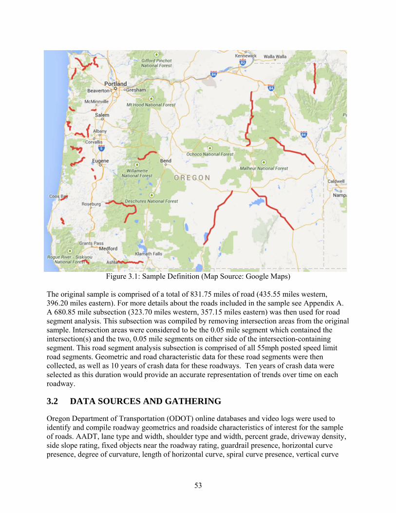
53

Figure 3.1: Sample Definition (Map Source: Google Maps) The original sample is comprised of a total of 831.75 miles of road (435.55 miles western, 396.20 miles eastern). For more details about the roads included in the sample see Appendix A. A 680.85 mile subsection (323.70 miles western, 357.15 miles eastern) was then used for road segment analysis. This subsection was compiled by removing intersection areas from the original sample. Intersection areas were considered to be the 0.05 mile segment which contained the intersection(s) and the two, 0.05 mile segments on either side of the intersection-containing segment. This road segment analysis subsection is comprised of all 55mph posted speed limit road segments. Geometric and road characteristic data for these road segments were then collected, as well as 10 years of crash data for these roadways. Ten years of crash data were selected as this duration would provide an accurate representation of trends over time on each roadway.

3.2 DATA SOURCES AND GATHERING

Oregon Department of Transportation (ODOT) online databases and video logs were used to identify and compile roadway geometrics and roadside characteristics of interest for the sample of roads. AADT, lane type and width, shoulder type and width, percent grade, driveway density, side slope rating, fixed objects near the roadway rating, guardrail presence, horizontal curve presence, degree of curvature, length of horizontal curve, spiral curve presence, vertical curve

54

presence and type, and length of vertical curve were determined for the sample with 0.05 mile resolution. The 0.05 mile resolution was selected because that increment allowed for video log data to be comprehensive without missing characteristics of interest between video log images. Ten years of crash records (2004 – 2013) from ODOT online databases were also gathered for the sample. Over 20 individual crash characteristics including crash location, road character, impact location, traffic control, crash type, crash severity and vehicle type involvement data were collected and combined with the geometric data into a unified database for analysis. The resulting comprehensive data set is very rich and includes all road characteristics described combined with all crash data for the 680.85 miles of low-volume state-owned roads in Oregon at 0.05 mile resolution. The database prepared for this purpose consists of over 13,000 records, each representing a 0.05 mile sub-segment with 62 individual road and crash characteristics for each sub-segment.

The data gathered in this effort were then used for data analysis which made the development of the risk index possible. The sample data were also used during the economic feasibility analysis task.

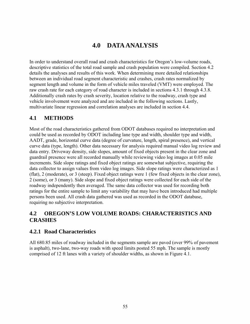
55

4.0 DATA ANALYSIS

In order to understand overall road and crash characteristics for Oregon’s low-volume roads, descriptive statistics of the total road sample and crash population were compiled. Section 4.2 details the analyses and results of this work. When determining more detailed relationships between an individual road segment characteristic and crashes, crash rates normalized by segment length and volume in the form of vehicle miles traveled (VMT) were employed. The raw crash rate for each category of road character is included in sections 4.3.1 through 4.3.8. Additionally crash rates by crash severity, location relative to the roadway, crash type and vehicle involvement were analyzed and are included in the following sections. Lastly, multivariate linear regression and correlation analyses are included in section 4.4.

4.1 METHODS

Most of the road characteristics gathered from ODOT databases required no interpretation and could be used as recorded by ODOT including lane type and width, shoulder type and width, AADT, grade, horizontal curve data (degree of curvature, length, spiral presence), and vertical curve data (type, length). Other data necessary for analysis required manual video log review and data entry. Driveway density, side slopes, amount of fixed objects present in the clear zone and guardrail presence were all recorded manually while reviewing video log images at 0.05 mile increments. Side slope ratings and fixed object ratings are somewhat subjective, requiring the data collector to assign values from video log images. Side slope ratings were characterized as 1 (flat), 2 (moderate), or 3 (steep). Fixed object ratings were 1 (few fixed objects in the clear zone), 2 (some), or 3 (many). Side slope and fixed object ratings were collected for each side of the roadway independently then averaged. The same data collector was used for recording both ratings for the entire sample to limit any variability that may have been introduced had multiple persons been used. All crash data gathered was used as recorded in the ODOT database, requiring no subjective interpretation.

4.2 OREGON’S LOW VOLUME ROADS: CHARACTERISTICS AND CRASHES

4.2.1 Road Characteristics

All 680.85 miles of roadway included in the segments sample are paved (over 99% of pavement is asphalt), two-lane, two-way roads with speed limits posted 55 mph. The sample is mostly comprised of 12 ft lanes with a variety of shoulder widths, as shown in Figure 4.1.

56

Figure 4.1: Sample Lane and Shoulder Widths Twenty percent (20%) of sample segments have no shoulders, 68% have pavement shoulders and 11% have gravel shoulders. There are no instances of “turf” shoulders recorded in the ODOT databases for the sample.

AADT categories indicate that the sample represents varying traffic levels under 1,000 vpd with around 65% of the sample having daily volumes less than 500 vpd. Additionally, driveway densities throughout the sample are also represented in an even manner from zero driveways to 7+ driveways per mile, as shown in Figure 4.2.

Figure 4.2: Sample AADT Ranges and Driveway Densities The sample includes fixed object ratings mostly in the few to some range, with the highest amount of fixed objects in the clear zone rating only comprising 2% of the total population. Similarly, very few roadway sections fell into the steepest side slope category with most represented in the moderate and flat side slope categories as shown in Figure 4.3.

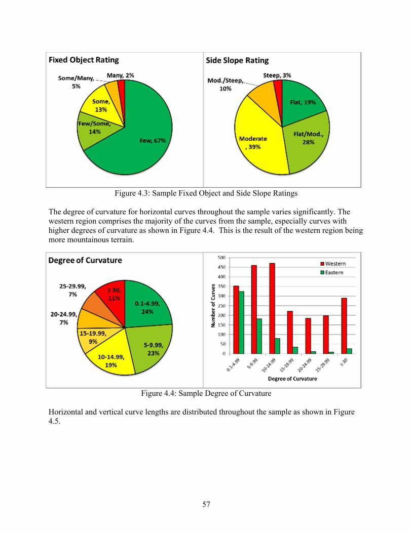
57

Figure 4.3: Sample Fixed Object and Side Slope Ratings The degree of curvature for horizontal curves throughout the sample varies significantly. The western region comprises the majority of the curves from the sample, especially curves with higher degrees of curvature as shown in Figure 4.4. This is the result of the western region being more mountainous terrain.

Figure 4.4: Sample Degree of Curvature Horizontal and vertical curve lengths are distributed throughout the sample as shown in Figure 4.5.

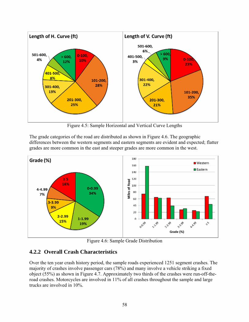
58

Figure 4.5: Sample Horizontal and Vertical Curve Lengths The grade categories of the road are distributed as shown in Figure 4.6. The geographic differences between the western segments and eastern segments are evident and expected; flatter grades are more common in the east and steeper grades are more common in the west.

Figure 4.6: Sample Grade Distribution

4.2.2 Overall Crash Characteristics

Over the ten year crash history period, the sample roads experienced 1251 segment crashes. The majority of crashes involve passenger cars (78%) and many involve a vehicle striking a fixed object (55%) as shown in Figure 4.7. Approximately two thirds of the crashes were run-off-the-road crashes. Motorcycles are involved in 11% of all crashes throughout the sample and large trucks are involved in 10%.

59

Figure 4.7: Crash Types and Vehicle Involvement The severities of crashes and driver involvement ages are shown in Figure 4.8.

Figure 4.8: Crash Severity and Driver Age Involvement Over half of all crashes (55%) involve some form of injury or a fatality. Young drivers, those under 20 years of age, are involved in 13% of crashes in the sample. Similarly 15% of crashes involved an elderly driver whose age was 65 or older.

Forty-two percent (42%) of crashes involved a driver that was within 25 miles of home, as shown in Figure 4.9. Crashes occurred most often on Saturdays compared to other days of the week.

60

Figure 4.9: Distance from Home and Day of Week Western region road segments experience higher traffic volumes, experience more crashes, and have higher crash rates than Eastern region road segments as shown in Table 4.1.

Table 4.1: Region Comparison Western Region Eastern Region

Length (miles) 323.70 357.15

Crashes 844 407

Ave. AADT (vpd) 580 382

Crashes/MVMT 1.23 0.82

4.3 CRASH OCCURRENCE AND ROAD CHARACTER RELATIONSHIPS

Roadway segment characteristics were examined individually to determine their potential effects on crash occurrence. The following eight sections detail the analysis results showing the relationships between road characteristics and the crashes observed on road segments between 2004 and 2013.

4.3.1 Lane Width

The majority of the roads in the sample have 12 foot lanes, but some segments have narrower lanes, down to 9 feet in some locations. Crash rates were observed to increase as lane widths narrowed, except for the 9-ft category. Figure 4.10 shows the crash rate (crashes per MVMT) observed for each lane width. Shaded columns in this figure and all following crash rate figures indicate that the rate for that category is based on a small sample size (less than 5% of the sample - 35 miles of road). Values based on small sample size may be less reliable than the other values. Crashes occur at a rate of 0.90 per MVMT when lanes are at least 12 feet wide, but increased to 1.48 for 10-ft lanes.

61

Figure 4.10: Crash Rate by Lane Width

The characteristics of crashes observed also tend to vary by the lane width category. Figure 4.11 shows the proportion of each crash characteristic (severity, on-road / off-road, type, and vehicle involvement) occurring by lane width category.

62

Figure 4.11: Crash Characteristics by Lane Width Crash severity relationships do not exhibit large differences across lane width categories. Lane width categories of 10 feet and greater experience 65% to 70% of crashes off the roadway, while 9 feet lanes experience 50% of crashes off the roadway. Fixed object crashes are the most common crash type occurring with 42% to 64% of crashes. Opposite direction crashes occur more often on 9 foot lanes (28%) and decrease with increasing lane width to a low of 5% on lanes 12 feet or wider. This trend may be attributed to the closer proximity that opposing vehicles must travel to one another on segments with a lower design standard. A similar but less obvious pattern is observed with the same direction collisions (e.g. sideswipe crashes). The type of vehicles involved in crashes also vary by lane width with passenger car only crashes being most common followed by motorcycle crashes (defined as those involving at least one motorcycle) and truck crashes (defined as those involving at least one large truck). It is evident that the narrowest roadways (9 foot lanes) have much higher instances of crashes involving motorcycles, and somewhat higher instances of crashes involving trucks when compared to the other lane width categories.

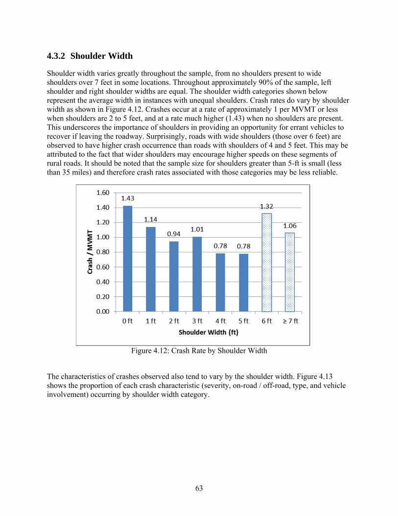
63

4.3.2 Shoulder Width

Shoulder width varies greatly throughout the sample, from no shoulders present to wide shoulders over 7 feet in some locations. Throughout approximately 90% of the sample, left shoulder and right shoulder widths are equal. The shoulder width categories shown below represent the average width in instances with unequal shoulders. Crash rates do vary by shoulder width as shown in Figure 4.12. Crashes occur at a rate of approximately 1 per MVMT or less when shoulders are 2 to 5 feet, and at a rate much higher (1.43) when no shoulders are present. This underscores the importance of shoulders in providing an opportunity for errant vehicles to recover if leaving the roadway. Surprisingly, roads with wide shoulders (those over 6 feet) are observed to have higher crash occurrence than roads with shoulders of 4 and 5 feet. This may be attributed to the fact that wider shoulders may encourage higher speeds on these segments of rural roads. It should be noted that the sample size for shoulders greater than 5-ft is small (less than 35 miles) and therefore crash rates associated with those categories may be less reliable.

Figure 4.12: Crash Rate by Shoulder Width

The characteristics of crashes observed also tend to vary by the shoulder width. Figure 4.13 shows the proportion of each crash characteristic (severity, on-road / off-road, type, and vehicle involvement) occurring by shoulder width category.

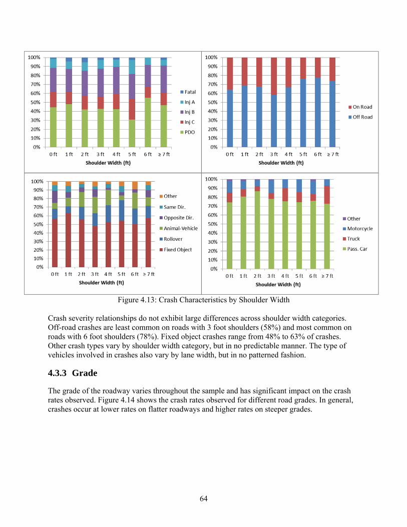
64

Figure 4.13: Crash Characteristics by Shoulder Width Crash severity relationships do not exhibit large differences across shoulder width categories. Off-road crashes are least common on roads with 3 foot shoulders (58%) and most common on roads with 6 foot shoulders (78%). Fixed object crashes range from 48% to 63% of crashes. Other crash types vary by shoulder width category, but in no predictable manner. The type of vehicles involved in crashes also vary by lane width, but in no patterned fashion.

4.3.3 Grade

The grade of the roadway varies throughout the sample and has significant impact on the crash rates observed. Figure 4.14 shows the crash rates observed for different road grades. In general, crashes occur at lower rates on flatter roadways and higher rates on steeper grades.

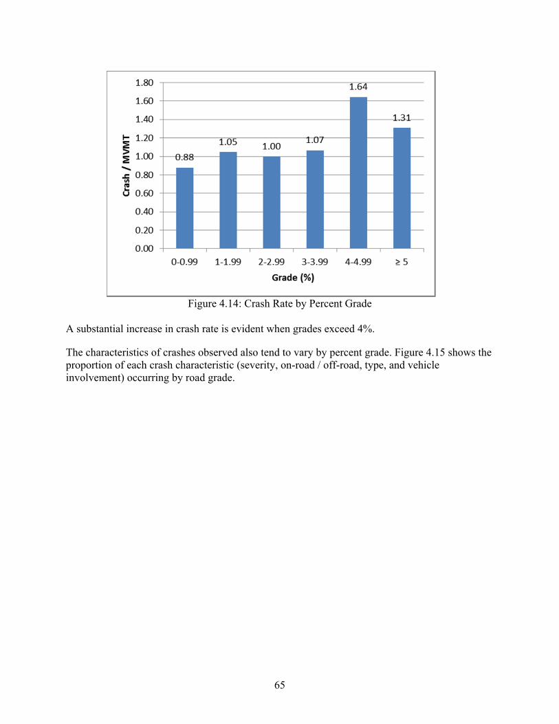
65

Figure 4.14: Crash Rate by Percent Grade

A substantial increase in crash rate is evident when grades exceed 4%.

The characteristics of crashes observed also tend to vary by percent grade. Figure 4.15 shows the proportion of each crash characteristic (severity, on-road / off-road, type, and vehicle involvement) occurring by road grade.

66

Figure 4.15: Crash Characteristics by Percent Grade Crash severity relationships vary by road grade, but not in a predictable fashion. Off-road crashes range from 64% (on the flattest road grades) to 74% (on road grades of 2-2.99%). Crash types vary by road grade in no discernable manner, except for opposite direction crashes which are least common on flatter grades (5%) and become increasingly common as grades increase up to 15% on the steepest grades category. The type of vehicles involved in crashes also vary by lane width, with truck and motorcycle crashes increasing with increasing road grade. This may be partly due to decreased stopping ability on downgrades as well as large speed differentials between trucks climbing grades and smaller vehicles.

4.3.4 Side Slope

Crashes occur at different rates depending upon the side slope rating of the roadway. Figure 4.16 shows the crash rates associated with the different side slope ratings from flatter (1) to steeper (3). It should be noted that the sample size for category 3 side slopes is small (less than 35 miles) and therefore crash rates associated with that category may be less reliable.

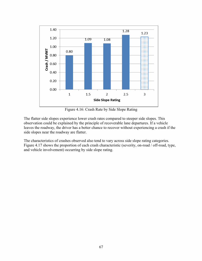
67

Figure 4.16: Crash Rate by Side Slope Rating

The flatter side slopes experience lower crash rates compared to steeper side slopes. This observation could be explained by the principle of recoverable lane departures. If a vehicle leaves the roadway, the driver has a better chance to recover without experiencing a crash if the side slopes near the roadway are flatter.

The characteristics of crashes observed also tend to vary across side slope rating categories. Figure 4.17 shows the proportion of each crash characteristic (severity, on-road / off-road, type, and vehicle involvement) occurring by side slope rating.

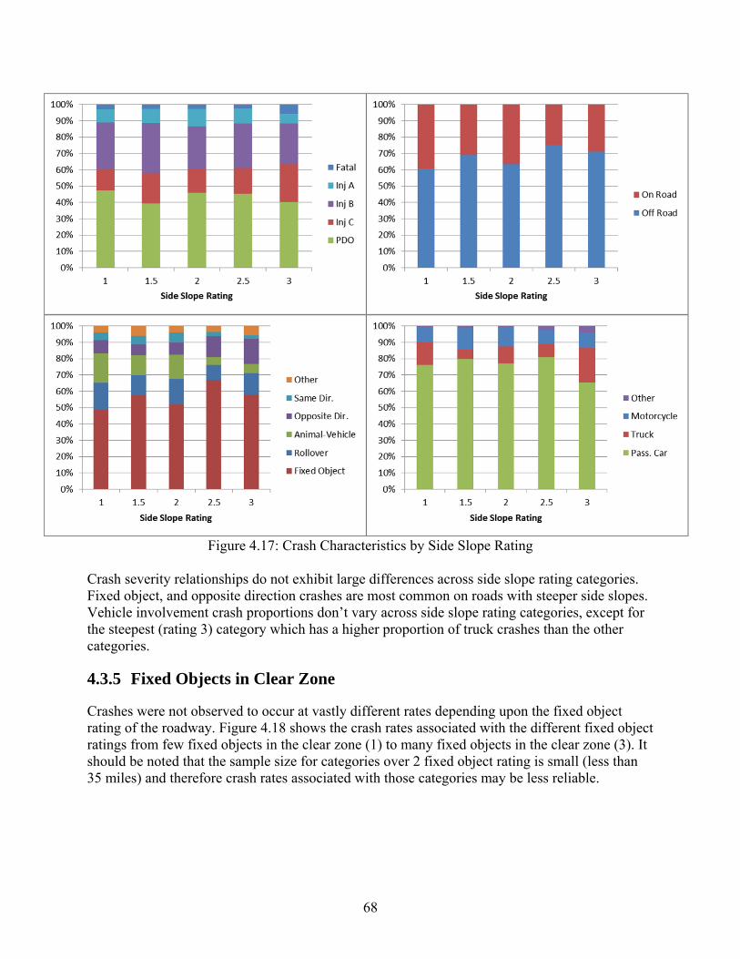
68

Figure 4.17: Crash Characteristics by Side Slope Rating Crash severity relationships do not exhibit large differences across side slope rating categories. Fixed object, and opposite direction crashes are most common on roads with steeper side slopes. Vehicle involvement crash proportions don’t vary across side slope rating categories, except for the steepest (rating 3) category which has a higher proportion of truck crashes than the other categories.

4.3.5 Fixed Objects in Clear Zone

Crashes were not observed to occur at vastly different rates depending upon the fixed object rating of the roadway. Figure 4.18 shows the crash rates associated with the different fixed object ratings from few fixed objects in the clear zone (1) to many fixed objects in the clear zone (3). It should be noted that the sample size for categories over 2 fixed object rating is small (less than 35 miles) and therefore crash rates associated with those categories may be less reliable.

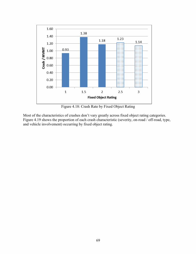
69

Figure 4.18: Crash Rate by Fixed Object Rating

Most of the characteristics of crashes don’t vary greatly across fixed object rating categories. Figure 4.19 shows the proportion of each crash characteristic (severity, on-road / off-road, type, and vehicle involvement) occurring by fixed object rating.

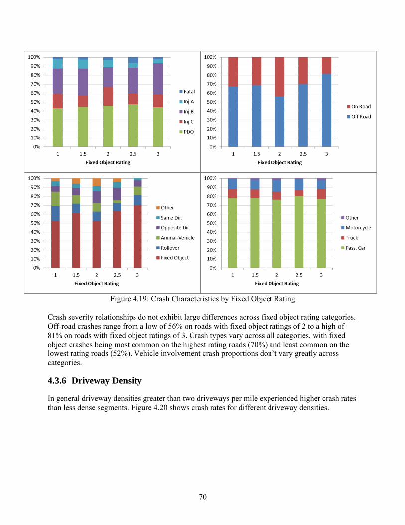
70

Figure 4.19: Crash Characteristics by Fixed Object Rating Crash severity relationships do not exhibit large differences across fixed object rating categories. Off-road crashes range from a low of 56% on roads with fixed object ratings of 2 to a high of 81% on roads with fixed object ratings of 3. Crash types vary across all categories, with fixed object crashes being most common on the highest rating roads (70%) and least common on the lowest rating roads (52%). Vehicle involvement crash proportions don’t vary greatly across categories.

4.3.6 Driveway Density

In general driveway densities greater than two driveways per mile experienced higher crash rates than less dense segments. Figure 4.20 shows crash rates for different driveway densities.

71

Figure 4.20: Crash Rate by Driveway Density

Most of the characteristics of crashes don’t vary greatly across driveway density categories. Figure 4.21 shows the proportion of each crash characteristic (severity, on-road / off-road, type, and vehicle involvement) occurring by driveway density.

72

Figure 4.21: Crash Characteristics by Driveway Density Crash severity relationships do not exhibit large differences across driveway density categories. Off-road crashes don’t exhibit any discernable crash proportion pattern by driveway density. Crash types vary across all categories, but again in no apparent pattern. Also vehicle involvement crash proportions don’t vary greatly by driveway density.

4.3.7 Horizontal Curves

The degree of curvature of horizontal curves has a large impact on crash rates. Figure 4.22 shows the crash rates for different degree of curvature categories. As curvature increases, crash rate increases from the lowest rate of 0.36 crashes per MVMT on curves with degree of curvature less than 5 degrees, up to 3.81 crashes per MVMT on curves with degree of curvature 30 or greater.

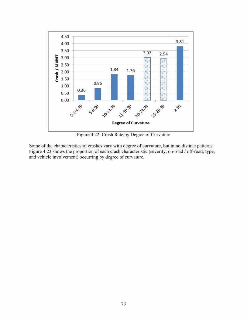
73

Figure 4.22: Crash Rate by Degree of Curvature

Some of the characteristics of crashes vary with degree of curvature, but in no distinct patterns. Figure 4.23 shows the proportion of each crash characteristic (severity, on-road / off-road, type, and vehicle involvement) occurring by degree of curvature.

74

Figure 4.23: Crash Characteristics by Degree of Curvature Crash severity relationships vary somewhat by degree of curvature, but in no discernable pattern. Off-road crashes don’t exhibit any discernable crash proportion pattern by degree of curvature. Crash types vary across all categories, but in no apparent pattern. Vehicle involvement crash proportions also vary by driveway density, but again in no discernable pattern.

Crash rates are also dependent on horizontal curve length. Figure 4.24 shows the observed crash rates for different horizontal curve length categories. Shorter curves tend to experience higher crash rates than longer curves. This is logical as longer curves present drivers with a more gradual roadway transition, potentially translating into a decreased risk of performing an errant maneuver resulting in a crash. It should be noted that the sample size for horizontal curves less than 100 feet is small (less than 15 miles of curves) and therefore crash rates associated with that category may be less reliable.

75

Figure 4.24: Crash Rate by Length of Horizontal Curve

Some of the crash characteristics vary by horizontal curve length but in no discernable pattern. Figure 4.25 shows the proportion of each crash characteristic (severity, on-road / off-road, type, and vehicle involvement) occurring by horizontal curve length.

76

Figure 4.25: Crash Characteristics by Length of Horizontal Curve

4.3.8 Vertical Curves

Crash rates are also dependent on vertical curve length. Figure 4.26 shows the crash rates observed for different vertical curve lengths. Shorter curves tend to experience higher crash rates than longer curves. It should be noted that the sample size for vertical curves 401 to 500 feet is small (less than 15 miles of curves) and therefore crash rates associated with that category may be less reliable.

77

Figure 4.26: Crash Rate by Length of Vertical Curve

Some of the characteristics of crashes vary with vertical curve length, but in no discernable pattern. Figure 4.27 shows the proportion of each crash characteristic (severity, on-road / off-road, type, and vehicle involvement) occurring by vertical curve length.

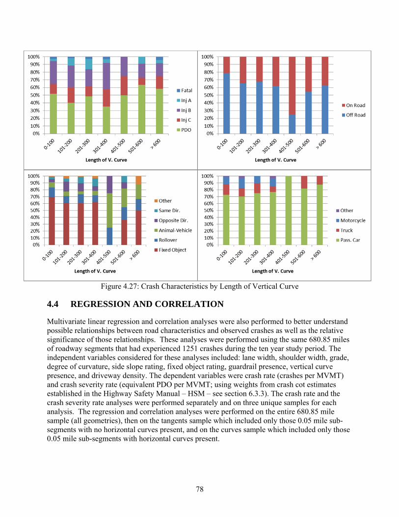
78

Figure 4.27: Crash Characteristics by Length of Vertical Curve

4.4 REGRESSION AND CORRELATION

Multivariate linear regression and correlation analyses were also performed to better understand possible relationships between road characteristics and observed crashes as well as the relative significance of those relationships. These analyses were performed using the same 680.85 miles of roadway segments that had experienced 1251 crashes during the ten year study period. The independent variables considered for these analyses included: lane width, shoulder width, grade, degree of curvature, side slope rating, fixed object rating, guardrail presence, vertical curve presence, and driveway density. The dependent variables were crash rate (crashes per MVMT) and crash severity rate (equivalent PDO per MVMT; using weights from crash cot estimates established in the Highway Safety Manual – HSM – see section 6.3.3). The crash rate and the crash severity rate analyses were performed separately and on three unique samples for each analysis. The regression and correlation analyses were performed on the entire 680.85 mile sample (all geometries), then on the tangents sample which included only those 0.05 mile sub-segments with no horizontal curves present, and on the curves sample which included only those 0.05 mile sub-segments with horizontal curves present.

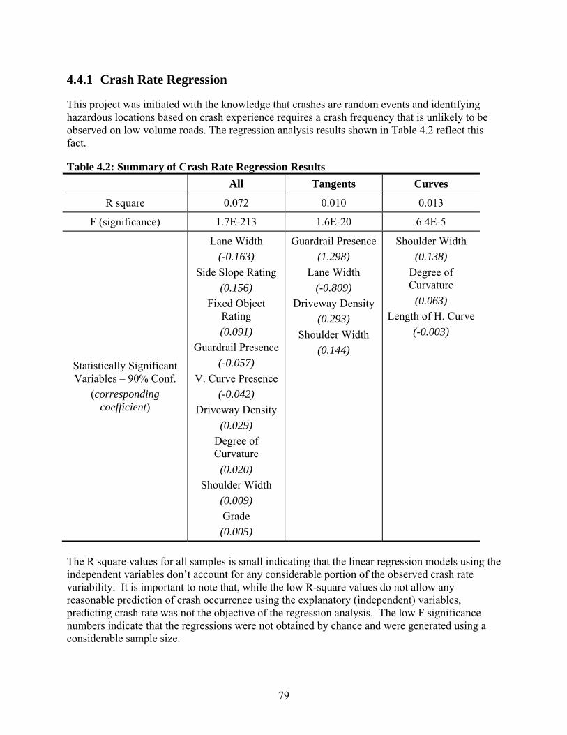
79

4.4.1 Crash Rate Regression

This project was initiated with the knowledge that crashes are random events and identifying hazardous locations based on crash experience requires a crash frequency that is unlikely to be observed on low volume roads. The regression analysis results shown in Table 4.2 reflect this fact.

Table 4.2: Summary of Crash Rate Regression Results

All Tangents Curves

R square 0.072 0.010 0.013

F (significance) 1.7E-213 1.6E-20 6.4E-5

Statistically Significant Variables – 90% Conf.

(corresponding coefficient)

Lane Width

(-0.163)

Side Slope Rating

(0.156)

Fixed Object Rating

(0.091)

Guardrail Presence

(-0.057)

V. Curve Presence

(-0.042)

Driveway Density

(0.029)

Degree of Curvature

(0.020)

Shoulder Width

(0.009)

Grade

(0.005)

Guardrail Presence

(1.298)

Lane Width

(-0.809)

Driveway Density

(0.293)

Shoulder Width

(0.144)

Shoulder Width

(0.138)

Degree of Curvature

(0.063)

Length of H. Curve

(-0.003)

The R square values for all samples is small indicating that the linear regression models using the independent variables don’t account for any considerable portion of the observed crash rate variability. It is important to note that, while the low R-square values do not allow any reasonable prediction of crash occurrence using the explanatory (independent) variables, predicting crash rate was not the objective of the regression analysis. The low F significance numbers indicate that the regressions were not obtained by chance and were generated using a considerable sample size.

80

All independent variables were found to be statistically significant at the 90% confidence level for all geometries. The signs (+ or -) of the regression coefficients of most of these variables suggest logical relationships with the dependent variable (i.e. crash rate). Specifically, increases in lane width correspond to decreases in crash rate and increases in side slope rating, fixed object rating, driveway density, degree of curvature, and grade all correspond to increases in crash rate. The presence of guardrail corresponds to a reduction in crash rate. The presence of vertical curves also corresponds to reductions in crash rate, a result that may be counterintuitive. Similarly, an increase in shoulder width corresponds to increases in crash rate which seems counterintuitive, but somewhat in agreement with the individual crash rate analysis for shoulder widths above 5 ft. Complete regression analysis results are included in Appendix B.

4.4.2 Crash Severity Rate Regression

Similar to the crash rate regression analysis, the crash severity rate regression analysis shows that the independent variables considered don’t explain much of the variability in the observed crash severity rates. Table 4.3 shows the results of the crash severity rate regression analysis.

Table 4.3: Summary of Crash Severity Rate Regression Results

All Tangents Curves

R square 0.005 0.007 0.003

F (significance) 5.1E-11 4.3E-13 6.3E-1

Statistically Significant Variables – 90% Conf.

(corresponding coefficient)

Fixed Object Rating

(9.47)

Guardrail Presence

(-5.14)

V. Curve Presence

(-3.40)

Side Slope Rating

(-2.71)

Lane Width

(2.22)

Shoulder Width

(-0.560)

Guardrail Presence

(42.85)

Lane Width

(-14.46)

Side Slope Rating

(-13.45)

Driveway Density

(6.90)

Shoulder Width

(2.61)

Degree of Curvature

(1.08)

The F significance numbers are low for all geometries and tangents, but exceed the 90% confidence level for the curves sample. Six of the independent variables (fixed object rating, guardrail presence, vertical curve presence, side slope rating, lane width, and shoulder width) were found to be statistically significant at the 90% confidence level for crash severity rate. The regression coefficients show that increases in fixed object rating correspond to increases in crash severity which is expected. Also the presence of guardrail corresponds to a reduction in crash severity which is also expected. Vertical curve presence corresponds to reduced crash severity

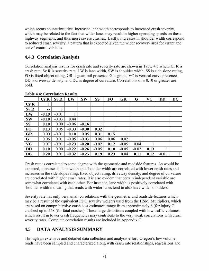
81

which seems counterintuitive. Increased lane width corresponds to increased crash severity, which may be related to the fact that wider lanes may result in higher operating speeds on these highway segments, and thus more severe crashes. Lastly, increases in shoulder width correspond to reduced crash severity, a pattern that is expected given the wider recovery area for errant and out-of-control vehicles.

4.4.3 Correlation Analysis

Correlation analysis results for crash rate and severity rate are shown in Table 4.5 where Cr R is crash rate, Sv R is severity rate, LW is lane width, SW is shoulder width, SS is side slope rating, FO is fixed object rating, GR is guardrail presence, G is grade, VC is vertical curve presence, DD is driveway density, and DC is degree of curvature. Correlations of ± 0.10 or greater are bold.

Table 4.4: Correlation Results Cr R Sv R LW SW SS FO GR G VC DD DC Cr R 1 Sv R -- 1 LW -0.19 -0.01 1 SW -0.10 -0.03 0.44 1 SS 0.10 0.00 -0.06 -0.16 1 FO 0.13 0.05 -0.33 -0.30 0.32 1 GR 0.00 -0.01 0.10 0.05 0.31 0.15 1 G 0.06 0.01 -0.05 -0.03 0.06 0.06 0.02 1 VC 0.07 -0.01 -0.23 -0.20 -0.02 0.12 -0.05 0.04 1 DD 0.10 0.00 -0.22 -0.26 -0.05 0.10 -0.05 -0.02 0.13 1 DC 0.20 0.01 -0.32 -0.25 0.19 0.23 0.04 0.11 0.12 -0.01 1

Crash rate is correlated to some degree with the geometric and roadside features. As would be expected, increases in lane width and shoulder width are correlated with lower crash rates and increases in the side slope rating, fixed object rating, driveway density, and degree of curvature are correlated with higher crash rates. It is also evident that certain independent variable are somewhat correlated with each other. For instance, lane width is positively correlated with shoulder width indicating that roads with wider lanes tend to also have wider shoulders.

Severity rate has only very small correlations with the geometric and roadside features which may be a result of the equivalent PDO severity weights used from the HSM. Multipliers, which are based on comprehensive crash cost estimates, range from approximately 6 (for injury C crashes) up to 568 (for fatal crashes). These large distortions coupled with low traffic volumes which result in lower crash frequencies may contribute to the very weak correlations with crash severity rates. Complete correlation results are included in Appendix C.

4.5 DATA ANALYSIS SUMMARY

Through an extensive and detailed data collection and analysis effort, Oregon’s low volume roads have been sampled and characterized along with crash rate relationships, regressions and

82

correlations in an effort to understand geometric and other roadway characteristics. This work has been done to determine what roadway characteristics may contribute to crash occurrence and aid in risk identification. The relationships established herein have aided other project tasks, especially Task 4 Risk Index Development, which develops a methodology for identifying safety hazards on low volume roads. The analyses conducted have shown which factors may influence crash risk and roughly the extent to which the risk may be increased for different situations. Table 4.5 shows a summary of the road characteristics and the resulting crash rate differences between categories of road character.

Table 4.5: Road Character Summary

Road Character Category Change Crash Rate Change

(Cr/MVMT)

Difference

(%)

Length of Horizontal Curve (ft) > 600 to ≤ 100 0.24 to 4.87 1929

Degree of Curvature < 5 to ≥ 30 0.36 to 3.81 958

Length of Vertical Curve (ft) > 600 to ≤ 100 0.34 to 3.38 894

Grade (%) < 1 to 4-5 0.88 to 1.64 86

Shoulder Width (ft) 4 to 0 0.78 to 1.43 83

Lane Width (ft) 12 to 10 0.90 to 1.48 64

Side Slope Rating 1 to 2.5 0.80 to 1.28 60

Driveway Density (driveways / mile) 1 to 5 0.84 to 1.34 60

Fixed Object Rating Variable Variable Variable

The difference in crash rate expressed in Table 4.5 is due partly to the road characteristics listed, but is also expected to be the result of multiple factors acting in conjunction. For example degree of curvature and length of horizontal curve are related and thus some of the difference in crash rate between degree of curvature categories may be due to curve length. Similarly, multiple road characteristics are expected to be present at any given location, and this makes it unrealistic to state that all of the change in a particular crash rate is due to a single characteristic. The regression analysis does consider multiple characteristics simultaneously and therefor may be a useful illustration showing multiple factors related to crash risk.

83

5.0 RISK INDEX DEVELOPMENT

This task’s goal was to develop a numerical index which could serve as an indicator of the level of risk associated with any particular site along low-volume roads. As defined earlier in this project, low-volume roads are roads with average daily traffic (ADT) of less than 1000 vpd. These roads usually consist of “secondary” two-lane highways serving less developed rural areas and are generally classified as class II two-lane highways per the Highway Capacity Manual (HCM) classification. The risk index developed and presented in this report can be used to assess the level of risk at any particular site along low-volume road segments and is not applicable to evaluating intersections alone. The geometric data gathered and analyzed in the previous project task are related to cross section characteristics of road segments.

5.1 GENERAL FORM

The proposed risk index considers three major elements that are known to influence the relative crash experience: geometric features, crash history, and traffic exposure. Each of the three major elements contributes to the overall crash risk as defined by the risk index shown in a general form:

(5.1)

Where:

is the crash risk index; a numerical expression of the relative crash risk,

is the geometric features weight; the contribution of geometric features to the total crash risk,

is the crash history weight; the contribution of crash history to the total crash risk,

is the traffic exposure weight; the contribution of traffic exposure to the total crash risk, and

, , are percentile scores which reflect site characteristics in regards to the three major elements; equations defined in the following sections.

While it may be argued that traffic level is more associated with crash frequency (as opposed to risk), it was included in the crash risk index to allow for using the index in ranking sites deserving safety countermeasures. Further, some phenomena associated with traffic level could affect crash risk (e.g. increased passing maneuvers on two-lane two-way highways could increase the risk of head-on collisions).

84

The weights used in the risk index formula should reflect agency priorities and preferences. For example, if only limited crash data are used, the weight used in this formulation could be lowered and more weights are assigned to the other two elements. For the purpose of this report, the weights used for geometric features, crash history and traffic exposure are 45%, 25%, and 30% respectively. Those weights were selected based on the engineering judgment of the research team. The resulting expression reflecting these weights is then:

. . . (5.2)

While the aforementioned weights were set based on the engineering judgment of the research team, ODOT respective staff have the choice to adopt those weights or adjust them to better reflect agency experience and other considerations.

5.2 GEOMETRIC FEATURES

The geometric features that contribute to increased crash risk for this risk index are included based on prior data analyses detailed in the Task 3 report for this project. The general form of the geometric features equation is:

(5.3)

Where: terms refer to weights associated with specific geometric features,

is degree of curvature; is length of vertical curve; is lane width; is grade; is shoulder width; is driveway density; is side slope rating; is fixed object rating

terms are numerical ratings associated with site geometric features and are defined in the Geometric Feature Values section of this document.

5.2.1 Geometric Feature Weights

The weights associated with each individual geometric and roadside feature were determined using the crash rate descriptive statistics and regression analyses. The weight of each geometric feature from the crash rate descriptive statistics analysis is set proportional to the deviation or difference in crash rates between the most restrictive value/rating of that geometric feature and the overall crash rate for the study sample. This method ensures that geometric features that exhibited larger influences on observed crash rates are weighted more heavily than those features that showed less influence on crash rates. The geometric feature weight from descriptive statistics is determined using the following formula:

∑

∗ % (5.4)

85

Where is the deviation/difference described earlier for geometric feature i. Length of horizontal curves and degree of curvature are not independent of each other, and therefore special consideration of their interrelatedness was necessary. The degree of curvature and length of horizontal curve relationship was further analyzed by varying one against the other in order to ensure that horizontal curve effects were not overestimated.

The weight of each geometric feature is also dependent upon the regression analysis results. In the regression analysis, all features were found to be significant in terms of explaining the variation in crash rates at the 90% confidence level, therefore all features have a regression weight associated with them. While the regression results found all features to be significant, the overall regression models did not adequately explain the crash rates observed in the data (i.e. models had very low coefficient of determination). For that reason, the regression results are deemed less reliable overall compared to the crash rate descriptive statistics analysis results. Therefore, in calculating the total geometric feature weight, it was deemed necessary for regression weights to have lower contribution compared to the weights found using descriptive statistics. The total resulting overall geometric feature weights are shown in Table 5.1. The total weight is calculated as a weighted average with the descriptive statistics weight column being 75% and the regression weight column being 25% of the total geometric feature weight.

Table 5.1: Overall Geometric Features Weights

Feature Rate Weight Regression Weight

Total

Degree of Curvature 43% 12.5% 36%

Length of Vertical Curve 37% 12.5% 30%

Lane Width 3% 12.5% 6%

Vertical Grade 4% 12.5% 6%

Shoulder Width 6% 12.5% 7%

Driveway Density 3% 12.5% 6%

Side Slope Rating 3% 12.5% 5%

Fixed Object Rating 1% 12.5% 4%

Total 100% 100% 100%

Using the proposed geometric feature weights the overall geometric features equation becomes:

. . . . . .. . (5.5)

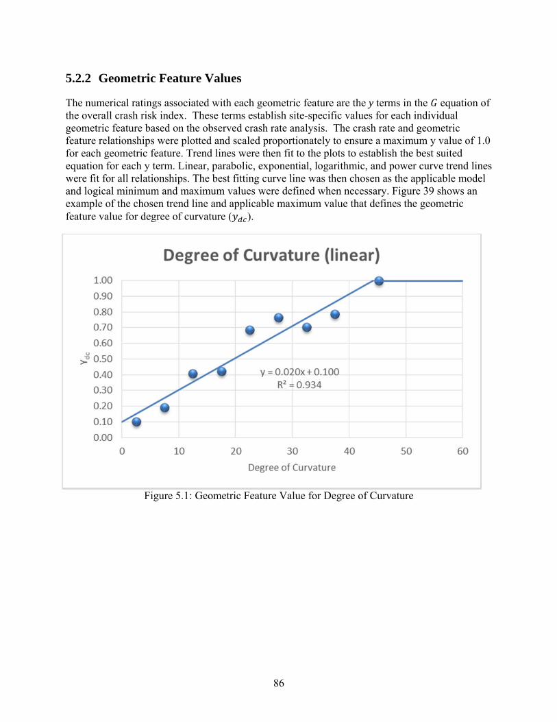
86

5.2.2 Geometric Feature Values

The numerical ratings associated with each geometric feature are the y terms in the equation of the overall crash risk index. These terms establish site-specific values for each individual geometric feature based on the observed crash rate analysis. The crash rate and geometric feature relationships were plotted and scaled proportionately to ensure a maximum y value of 1.0 for each geometric feature. Trend lines were then fit to the plots to establish the best suited equation for each y term. Linear, parabolic, exponential, logarithmic, and power curve trend lines were fit for all relationships. The best fitting curve line was then chosen as the applicable model and logical minimum and maximum values were defined when necessary. Figure 39 shows an example of the chosen trend line and applicable maximum value that defines the geometric feature value for degree of curvature ( ).

Figure 5.1: Geometric Feature Value for Degree of Curvature

87

The equations of all geometric features are shown in Table 5.2.

Table 5.2: Equations for Geometric and Roadside Features Geometric Feature Equation Condition

Degree of Curvature 0.029 ∗ 0.033 1.00 0.00

dc ≤ 33 dc > 33 no horizontal curve present

Length of Vertical Curve 0.365 ∗ ln 2.386 1.00 0.00 0.00

50 ft ≤ lvc ≤ 690 ft lvc < 50 ft lvc > 690 ft no vertical curve present

Lane Width 0.110 ∗ 2.227 ∗

10.270 0.86 0.61

9 ft ≤ lw ≤ 12 ft lw < 9 ft lw > 12 ft

Grade 0.510 . ∗ 1.00

g ≤ 7% g > 7%

Shoulder Width 0.025 ∗ 0.199 ∗

1.000 0.83

sw ≤ 7 ft sw > 7 ft

Driveway Density 0.010 ∗ 0.125 ∗

0.611 1.00

dd ≤ 7 driveways/mile dd > 7 driveways/mile

Side Slope 0.106 ∗ 0.593 ∗

0.173

all ss ratings

Fixed Object Rating 0.181 ∗ 0.763 ∗

0.195

all fo ratings

The term, which defines the geometric component of the CRI, is scaled as a result of investigating the range of possible values for the entire 680.85 mile sample. The average and standard deviation of the term for the sample was found to be 0.32 and 0.121 respectively. The scale is defined as shown in Figure 5.2 such that one standard deviation below the mean is = 0 and three standard deviations above the mean is = 1.

88

Figure 5.2: XG Definition Geometric Features (XG)

2.083 ∗ 0.417 [0.20 ≤ G ≤ 0.68],

0.00 [G < 0.20], or

1.00 [G > 0.68].

5.3 CRASH HISTORY

The crash history risk index values are based on the average crash rate and the critical crash rate for the sample low-volume roads as defined in the Highway Safety Manual (10). The average crash rate for the sample was found to be 1.06 crashes per MVMT (million vehicle miles traveled). The critical rate is dependent upon the average rate at similar sites, traffic volume, and a statistical level of confidence associated with the Poisson distribution and can be estimated using the following equation:

/ ⁄ (5.6)

Where Rc is the critical crash rate, Ra is the average crash rate at similar locations, k is a constant determined by the confidence interval, and E is traffic exposure.

The average critical rate for all segments of the low-volume roads sample was found to be 2.52 crashes per MVMT for 90% confidence level. Data over the most recently available 10 year

89

period (2004 – 2013) was used in determining the average and critical rates. The minimum crash rate is selected as the half of the average crash rate and the maximum crash rate is selected as the average critical rate for 90% confidence level. Figure 5.3 shows the crash history risk index value model using a linear relationship.

Figure 5.3: Crash History Value Crash History (Xc)

0.502 ∗ 0.266 [0.53 ≤ crash rate ≤ 2.52],

0.00 [crash rate < 0.53], or

1.00 [crash rate > 2.52].

Crash history values used for calculation in the CRI should be a rolling 1 mile value in order to be consistent with the data analysis methods used and to accommodate the reality that crash data reported mile posts may not be accurate to very small resolutions.

5.4 TRAFFIC EXPOSURE

The proposed crash risk index considers two aspects of traffic exposure in estimating the exposure risk index values: total vehicular traffic volume expressed as average daily traffic (ADT) and the percentage of heavy vehicles in the traffic stream (AASHTO class 4 or larger). The fundamental relationship underlying this component of the CRI is that crash risk increases with the increase of total vehicular volume as well as with the increase in the percentage of heavy vehicles. The average percentage of heavy vehicles for the low-volume roads sample used in this study was found to be approximately 29% of the total traffic volume. The standard deviation of the percentage of heavy vehicles for the sample was found to be approximately

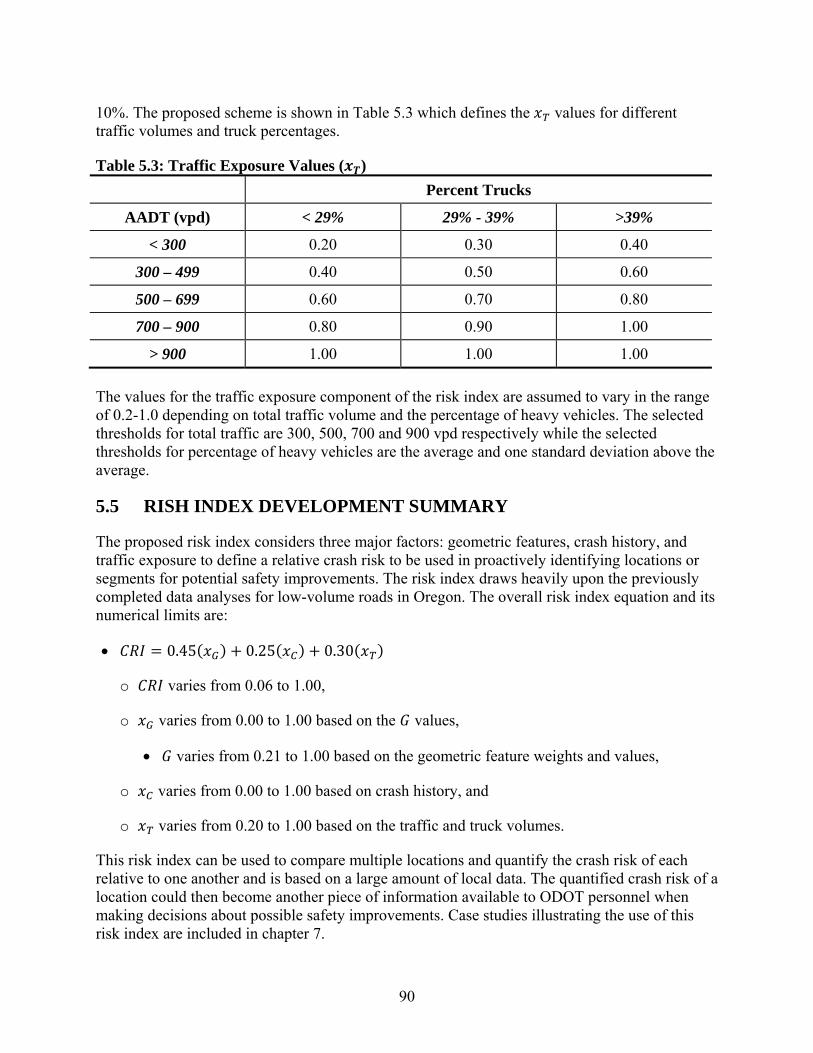
90

10%. The proposed scheme is shown in Table 5.3 which defines the values for different traffic volumes and truck percentages.

Table 5.3: Traffic Exposure Values ( )

Percent Trucks

AADT (vpd) < 29% 29% - 39% >39%

< 300 0.20 0.30 0.40

300 – 499 0.40 0.50 0.60

500 – 699 0.60 0.70 0.80

700 – 900 0.80 0.90 1.00

> 900 1.00 1.00 1.00

The values for the traffic exposure component of the risk index are assumed to vary in the range of 0.2-1.0 depending on total traffic volume and the percentage of heavy vehicles. The selected thresholds for total traffic are 300, 500, 700 and 900 vpd respectively while the selected thresholds for percentage of heavy vehicles are the average and one standard deviation above the average.

5.5 RISH INDEX DEVELOPMENT SUMMARY

The proposed risk index considers three major factors: geometric features, crash history, and traffic exposure to define a relative crash risk to be used in proactively identifying locations or segments for potential safety improvements. The risk index draws heavily upon the previously completed data analyses for low-volume roads in Oregon. The overall risk index equation and its numerical limits are:

0.45 0.25 0.30

o varies from 0.06 to 1.00,

o varies from 0.00 to 1.00 based on the values,

varies from 0.21 to 1.00 based on the geometric feature weights and values,

o varies from 0.00 to 1.00 based on crash history, and

o varies from 0.20 to 1.00 based on the traffic and truck volumes.

This risk index can be used to compare multiple locations and quantify the crash risk of each relative to one another and is based on a large amount of local data. The quantified crash risk of a location could then become another piece of information available to ODOT personnel when making decisions about possible safety improvements. Case studies illustrating the use of this risk index are included in chapter 7.

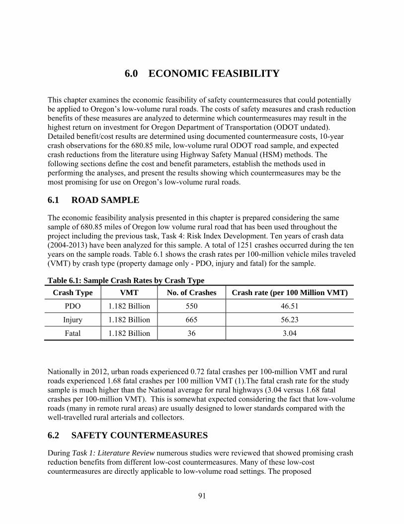
91

6.0 ECONOMIC FEASIBILITY

This chapter examines the economic feasibility of safety countermeasures that could potentially be applied to Oregon’s low-volume rural roads. The costs of safety measures and crash reduction benefits of these measures are analyzed to determine which countermeasures may result in the highest return on investment for Oregon Department of Transportation (ODOT undated). Detailed benefit/cost results are determined using documented countermeasure costs, 10-year crash observations for the 680.85 mile, low-volume rural ODOT road sample, and expected crash reductions from the literature using Highway Safety Manual (HSM) methods. The following sections define the cost and benefit parameters, establish the methods used in performing the analyses, and present the results showing which countermeasures may be the most promising for use on Oregon’s low-volume rural roads.

6.1 ROAD SAMPLE

The economic feasibility analysis presented in this chapter is prepared considering the same sample of 680.85 miles of Oregon low volume rural road that has been used throughout the project including the previous task, Task 4: Risk Index Development. Ten years of crash data (2004-2013) have been analyzed for this sample. A total of 1251 crashes occurred during the ten years on the sample roads. Table 6.1 shows the crash rates per 100-million vehicle miles traveled (VMT) by crash type (property damage only - PDO, injury and fatal) for the sample.

Table 6.1: Sample Crash Rates by Crash Type

x

Crash Type VMT No. of Crashes Crash rate (per 100 Million VMT)

PDO 1.182 Billion 550 46.51

Injury 1.182 Billion 665 56.23

Fatal 1.182 Billion 36 3.04

Nationally in 2012, urban roads experienced 0.72 fatal crashes per 100-million VMT and rural roads experienced 1.68 fatal crashes per 100 million VMT (1).The fatal crash rate for the study sample is much higher than the National average for rural highways (3.04 versus 1.68 fatal crashes per 100-million VMT). This is somewhat expected considering the fact that low-volume roads (many in remote rural areas) are usually designed to lower standards compared with the well-travelled rural arterials and collectors.

6.2 SAFETY COUNTERMEASURES

During Task 1: Literature Review numerous studies were reviewed that showed promising crash reduction benefits from different low-cost countermeasures. Many of these low-cost countermeasures are directly applicable to low-volume road settings. The proposed

92

countermeasures considered for this economic feasibility analysis are separated into four categories based on the types of risks they mitigate: 1) highway alignment, 2) roadway cross section, 3) roadside features, and 4) other countermeasures. Only those countermeasures with usable quantified crash reduction benefits are included, as the benefits are required to perform the economic analyses.

Highway Alignment

Altering the geometry of the road to mitigate risks associated with the road alignment is costly, but some lower cost alignment warning countermeasures have been successfully used. These countermeasures do not improve the physical layout of the road, but rather warn the driver of the presence of curves that may be unexpected. These low-cost treatments include:

Horizontal Alignment Signs

Horizontal Alignment Signs with Static Advisory Speeds

Flashing Beacons for Curve Warning

Chevrons

Post Mounted Delineators for Curves

Raised Pavement Markers (Curves and Other Features)

Dynamic Speed Feedback Displays on Approach to Curves

High Friction Surface Treatments for Curves

Roadway Cross Section

Safety treatments that improve the roadway cross section can also be costly, but some moderate to low-cost options have been proposed for analysis. Adding, widening, or improving shoulders and lanes as well as improving the surface friction of the road can lead to crash reductions. The specific treatments documented and considered for this analysis include:

Widen Lanes

Widen Paved Shoulders

Widen Un-Paved Shoulders

Adding Paved Shoulders

Stabilizing Shoulders

High Friction Surface Treatments

93

Roadside Features Roadside features can also be improved using low-cost countermeasures. Edge drops, side slopes, and features in the clear-zone can all influence crash risk and severity. The specific treatments for roadside features proposed are:

Flatten Side Slopes

Install Safety Edge

Improve Roadside Hazard Rating

Install Object Markers for Objects Near the Roadway

Relocate Objects Near the Roadway

Remove Objects Near the Roadway

Other Countermeasures A handful of other countermeasures that don’t fit into the prior categories are also considered for analysis. These treatments include:



Install Edge-line Markings

Install Centerline Markings

Install Edge-line and Centerline Markings

Widen Edge-line Markings

Widen Centerline Markings

6.3 BENEFIT-COST ANALYSIS

To determine the economic feasibility of the proposed safety measures, both the costs of the treatments and the benefits reasonably expected from those treatments need to be established. The overall benefit-to-cost ratios (B/C) can then be determined to provide guidance on which treatments may be the best use of agency funds.

94

6.3.1 Costs of Countermeasures

Comprehensive and up-to-date cost information for all the proposed safety measures was challenging to find, but an FHWA report (Atkinson et al. 2014), ODOT (ODOT 2014), Florida Department of Transportation, FDOT (Davis 2015), and Texas Department of Transportation, TxDOT (McDaniel 2015) all provided useful figures to complete the cost data when other published sources could not be found. Table 6.2. shows the alignment treatment costs and any associated maintenance and life cycle replacement type costs to arrive at an average equivalent 1-year cost that is used in the economic analysis. Initial costs are amortized over 10 years when necessary for calculations. For all cost tables the initial cost sources are referenced individually, and all maintenance / life cycle type costs are from the FHWA report (Atkinson et al. 2014) unless otherwise noted. In reality many of the treatment cost could vary greatly from the numbers given due to local factors and circumstances. All costs are approximate and rounded to the nearest hundred dollars. Cost are adjusted for inflation to represent 2015 dollars using US Bureau of Labor Statistics, Consumer Price Index methods.

95

Table 6.2: Costs of Alignment Safety Measures

x

Treatment (Reference) Initial Cost Maintenance / Life Cycle Cost

Average Equivalent 1 Year Cost

Horizontal Alignment Sign (Davis 2015; McDaniel 2015)

$300 to $3,500 per installation

$1,300 / 5 years $500

Horizontal Alignment Sign with Static Advisory Speed (Davis 2015; McDaniel 2015)


$1,300 / 5 years $500

Flashing Beacon for Curve Warning (Sperry et al. 2008)

$2,400 per installation

$1,000 / 2 years $700

Chevrons (McGee and Hanscom 2006; Atkinson et al. 2014)


$3,600 / 5 years $1,100

Post Mounted Delineators for Curves (Atkinson et al. 2014)

$5,600 per installation

Life ≥ 10 years $600

Raised Pavement Markers for Curves (Jiang 2006)

$6001 per installation

$600 / 2 years (Error! Bookmark

not defined.) $400

Dynamic Speed Feedback Display on Approach to Curves (Hallmark et al. 2007; Davis 2015)

$2,300 to $12,600 per installation

$1,0002 / 2 years $1,200

High Friction Surface Treatment for Curves (Davis 2015; McDaniel 2015)

$13,6003 to $18,700 Life ≥ 10 years $1,600

Most alignment related safety measures are inexpensive with 1-year costs under $1,600.

1 Calculated for a 500 foot horizontal curve and 40 foot marker spacing. 2 No value given, but assumed to be equal to or greater than beacon maintenance. 3 Calculated for a 500 foot horizontal curve with two 12-foot lanes, 1 inch mill, and 1 inch overlay.

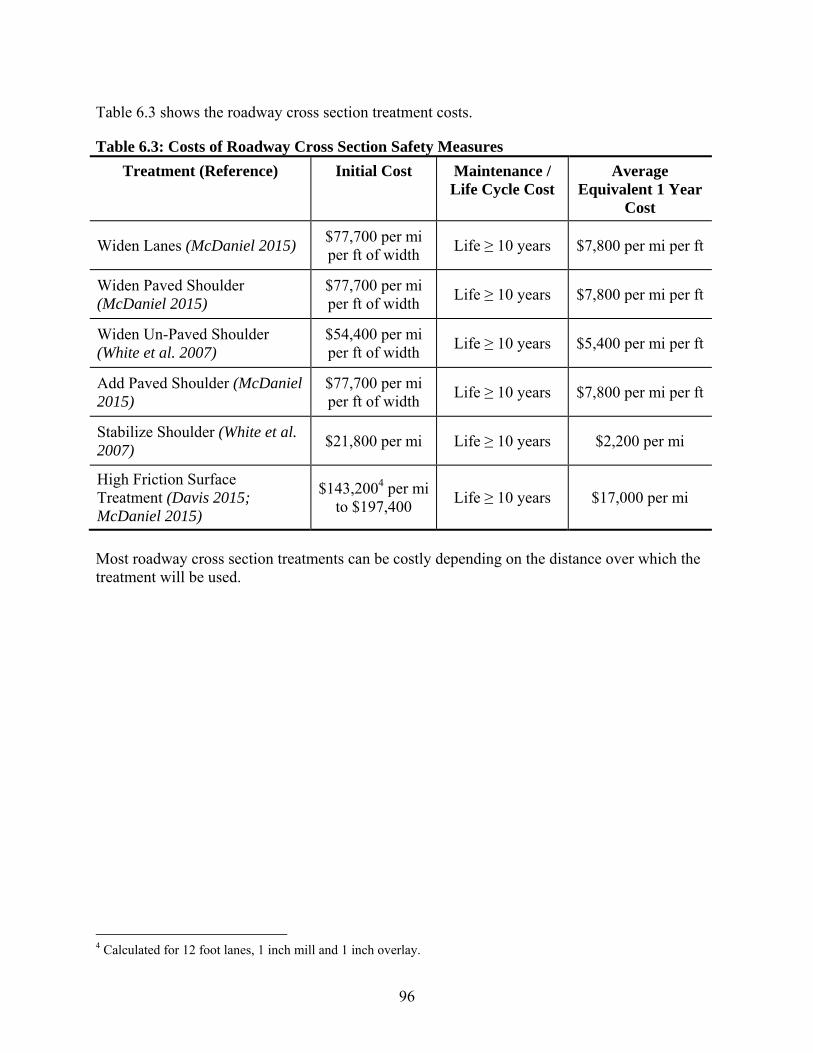
96

Table 6.3 shows the roadway cross section treatment costs.

Table 6.3: Costs of Roadway Cross Section Safety Measures

x


Average Equivalent 1 Year

Cost

Widen Lanes (McDaniel 2015) $77,700 per mi per ft of width

Life ≥ 10 years $7,800 per mi per ft

Widen Paved Shoulder (McDaniel 2015)

$77,700 per mi per ft of width


Widen Un-Paved Shoulder (White et al. 2007)



Add Paved Shoulder (McDaniel 2015)



Stabilize Shoulder (White et al. 2007)

$21,800 per mi Life ≥ 10 years $2,200 per mi

High Friction Surface Treatment (Davis 2015; McDaniel 2015)

$143,2004 per mi to $197,400

Life ≥ 10 years $17,000 per mi

Most roadway cross section treatments can be costly depending on the distance over which the treatment will be used.

4 Calculated for 12 foot lanes, 1 inch mill and 1 inch overlay.

97

Table 6.4 shows the roadside feature treatment costs.

Table 6.4: Costs of Roadside Features Safety Measures

x



Cost

Flatten Side Slopes (Davis 2015) $34,9005 per mi Life ≥ 10 years $3,500 per mi

Install Safety Edge (Graham et al. 2011)

$500 to $2,300 per mi

Life > 10 years $150 per mi

Improve Roadside Hazard Rating (McDaniel 2015)

$103,000 per mi Life > 10 years $10,300 per mi

Install Object Markers for Objects Near the Roadway (Davis 2015)

$5,300 to $8,5006 per mi

Life > 10 years $700 per mi

Relocate Objects Near the Roadway (McDaniel 2015)


Remove Objects Near the Roadway (McDaniel 2015)


Some of the roadside features countermeasures are low-cost while others can be more expensive, and they are also highly dependent on treatment length.

5 Calculated for 3:1 to 6:1 flattening 30 ft width. 6 Calculated assuming 1 marked object every 100 ft.

98

Table 6.5 shows the treatment costs for the countermeasures in the other category.

Table 6.5: Costs of Other Safety Measures

x



Cost

Install Shoulder Rumble Strips (McGee and Hanscom 2006)

$2,100 per mi Life > 10 years $200 per mi

Install Centerline Rumble Strips (McGee and Hanscom 2006)

$2,100 per mi Life > 10 years $200 per mi

Install Edge-line Markings (Massachusetts Traffic Safety Toolbox Series 2008)

$1,800 to $5,000 per mi per line

$3,400 / 3 years $1,500 per mi

Install Centerline Markings (Massachusetts Traffic Safety Toolbox Series 2008)


$3,400 / 3 years $1,500 per mi

Install Edge-line and Centerline Markings (Massachusetts Traffic Safety Toolbox Series 2008)


$3,400 / 3 years $1,500 per mi

Widen Edge-line Markings (Davis 2015)

$4,300 per mi per line

$4,300 / 3 years $1,900 per mi

Widen Centerline Markings (Davis 2015)

$4,300 per mi per line

$4,300 / 3 years $1,900 per mi

Most of the safety countermeasures in the other category are low cost per mile compared to roadway cross section and roadside feature treatments.

6.3.2 Benefits of Countermeasures

Literature reviewed during Task 1: Literature Review uncovered many crash reduction benefits for the safety countermeasures considered in this economic analysis. These benefits are expressed as crash reduction factors (CRFs) that represent the proportion of total crashes that can be expected to be avoided by using the treatment. Some of the measures also have documented CRFs for different severity levels of crashes be they property damage only (PDO), injury, or fatal. The CRFs included here are meant to be estimates using the best information available. As is common with most CRFs, local factors present during the studies can have great influence on the reported values, and vagueness in reporting can also affect the applicability of these values to this study. Table 6.6 shows the CRF benefits for the alignment safety countermeasures. When CRF ranges are cited, the average value is used for benefit-to-cost calculations.

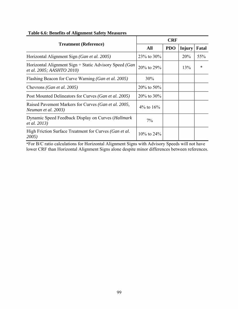
99

Table 6.6: Benefits of Alignment Safety Measures

*For B/C ratio calculations for Horizontal Alignment Signs with Advisory Speeds will not have lower CRF than Horizontal Alignment Signs alone despite minor differences between references. x

Treatment (Reference) CRF

All PDO Injury Fatal

Horizontal Alignment Sign (Gan et al. 2005) 23% to 30% 20% 55%

Horizontal Alignment Sign + Static Advisory Speed (Gan et al. 2005; AASHTO 2010)

20% to 29% 13% *

Flashing Beacon for Curve Warning (Gan et al. 2005) 30%

Chevrons (Gan et al. 2005) 20% to 50%

Post Mounted Delineators for Curves (Gan et al. 2005) 20% to 30%

Raised Pavement Markers for Curves (Gan et al. 2005, Neuman et al. 2003)

4% to 16%

Dynamic Speed Feedback Display on Curves (Hallmark et al. 2013)

7%

High Friction Surface Treatment for Curves (Gan et al. 2005)

10% to 24%

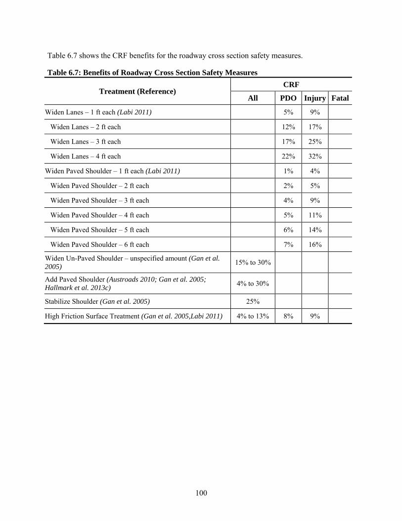
100

Table 6.7 shows the CRF benefits for the roadway cross section safety measures.

Table 6.7: Benefits of Roadway Cross Section Safety Measures

x



Widen Lanes – 1 ft each (Labi 2011) 5% 9%

Widen Lanes – 2 ft each 12% 17%



Widen Paved Shoulder – 1 ft each (Labi 2011) 1% 4%

Widen Paved Shoulder – 2 ft each 2% 5%





Widen Un-Paved Shoulder – unspecified amount (Gan et al. 2005)

15% to 30%

Add Paved Shoulder (Austroads 2010; Gan et al. 2005; Hallmark et al. 2013c)

4% to 30%

Stabilize Shoulder (Gan et al. 2005) 25%

High Friction Surface Treatment (Gan et al. 2005,Labi 2011) 4% to 13% 8% 9%

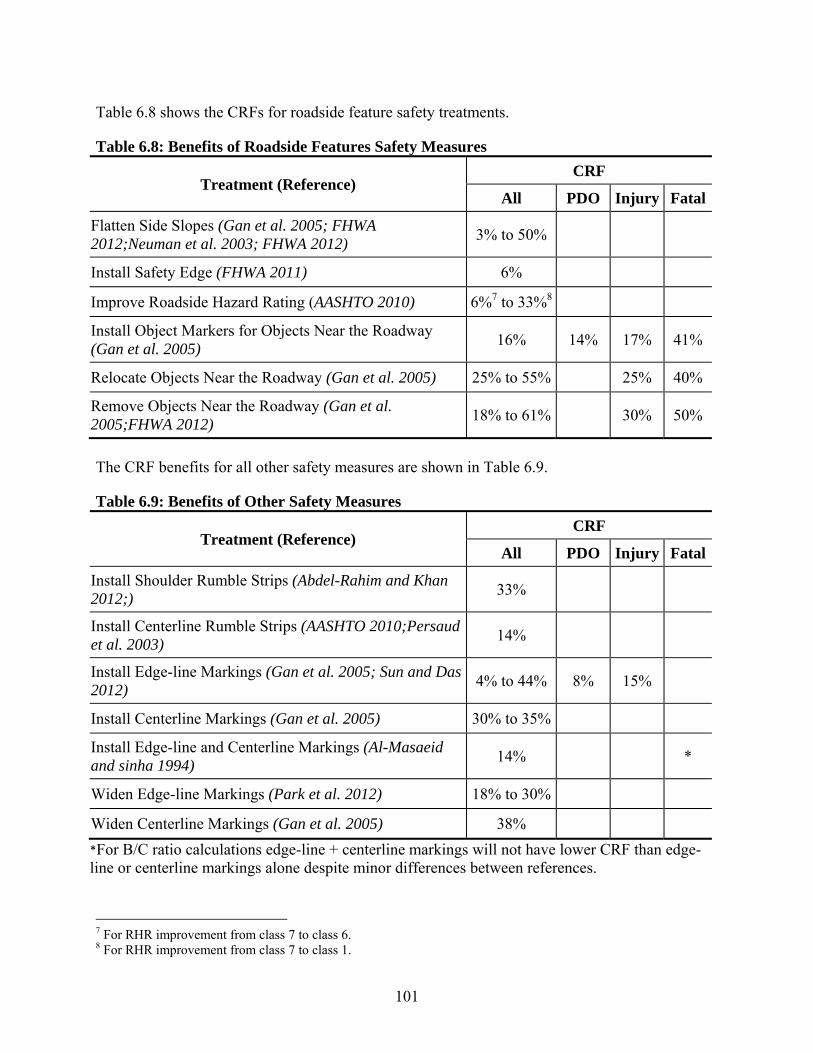
101

Table 6.8 shows the CRFs for roadside feature safety treatments.

Table 6.8: Benefits of Roadside Features Safety Measures

x



Flatten Side Slopes (Gan et al. 2005; FHWA 2012;Neuman et al. 2003; FHWA 2012)

3% to 50%

Install Safety Edge (FHWA 2011) 6%

Improve Roadside Hazard Rating (AASHTO 2010) 6%7 to 33%8

Install Object Markers for Objects Near the Roadway (Gan et al. 2005)

16% 14% 17% 41%

Relocate Objects Near the Roadway (Gan et al. 2005) 25% to 55% 25% 40%

Remove Objects Near the Roadway (Gan et al. 2005;FHWA 2012)

18% to 61% 30% 50%

The CRF benefits for all other safety measures are shown in Table 6.9.

Table 6.9: Benefits of Other Safety Measures

*For B/C ratio calculations edge-line + centerline markings will not have lower CRF than edge-line or centerline markings alone despite minor differences between references. x



Install Shoulder Rumble Strips (Abdel-Rahim and Khan 2012;)

33%

Install Centerline Rumble Strips (AASHTO 2010;Persaud et al. 2003)

14%

Install Edge-line Markings (Gan et al. 2005; Sun and Das 2012)

4% to 44% 8% 15%

Install Centerline Markings (Gan et al. 2005) 30% to 35%

Install Edge-line and Centerline Markings (Al-Masaeid and sinha 1994)

14% *

Widen Edge-line Markings (Park et al. 2012) 18% to 30%

Widen Centerline Markings (Gan et al. 2005) 38%

7 For RHR improvement from class 7 to class 6. 8 For RHR improvement from class 7 to class 1.

102

6.3.3 Benefit / Cost Relationships

The crash reduction benefits of the safety countermeasures can be quantified in monetary value using agency defined crash cost equivalencies for different crash severities. Table 6.10 shows the crash costs for different crash types as defined by both ODOT and the American Association of State Highway and Transportation Officials (AASHTO) in the Highway Safety Manual (HSM). More recent FHWA “value of statistical life” methods are not used here as those values use a six tier Abbreviated Injury Scale severity system which does not match well with the crash data used for analysis. Costs are adjusted for inflation to represent 2015 dollars using US Bureau of Labor Statistics, Consumer Price Index and Employment Cost Index methods as suggested in the HSM.

Table 6.10: Crash Costs x Crash Type ODOT Cost9 (ODOT

undated) HSM Cost (AASHTO

2010)

PDO $20,237 $10,040

Injury C $85,884

$62,153

Injury B $110,313

Injury A $1,766,395

$301,989

Fatal $5,702,325

The ODOT crash costs have fatal and injury type-A crashes combined, which is slightly different than the HSM values used which have separate costs for fatal and injury crashes. Also ODOT data has injury B and injury C costs combined.

Some safety treatments are targeted toward curves while others are applied to all road type segments. For benefit/cost analyses, the crash reduction cost savings for possible alignment safety measures are applied to all horizontal curves in the sample. All other safety treatments are targeted toward all road segments and the cost reduction benefits for those are therefore applied to all of the road sample. Table 6.11 shows the samples with crash characteristics and total 10-year equivalent crash costs.

Table 6.11: Estimated Crash Costs on Road Sample

x

Sample Quantity 10 Year Crash Total ODOT

Cost HSM Cost PDO Inj C Inj B Inj A Fatal Total

Curves 2841 curves 145 66 120 36 8 375 $96.6M $75.3M

All 680.85 miles 550 199 349 117 36 1251 $328.5M $297.0M

To determine the potential crash reduction benefits for each treatment, the number of crashes prevented for each crash type per unit (either curve of mile of road) is calculated using the

9 Rural, non-Interstate, State Highway values

103

CRFs10. Then each treatment’s benefit can be calculated using the number of crashes prevented and the cost of each type of crash. This resulting 10-year unit benefit can then be normalized to 1 year benefits for comparison to the 1-year unit cost for each treatment to calculate the B/C ratios. For more detailed B/C calculations see Appendix E. Table 6.12 shows the benefit/cost ratios for the alignment safety measures using both ODOT and HSM crash cost estimates. For all B/C ratio tables, ratios greater than 1 are in bold and underlined.

Table 6.12: Benefit/Costs Ratios of Alignment Safety Measures

x

Treatment B/C (ODOT Values)

B/C (HSM Values)

Horizontal Alignment Sign (Gan et al. 2005) 1.64 1.10

Horizontal Alignment Sign with Static Advisory Speed (Gan et al. 2005; AASHTO 2010)

1.64 1.10

Flashing Beacon for Curve Warning (Gan et al. 2005)

1.46 1.14

Chevrons (Gan et al. 2005) 1.08 0.84

Post Mounted Delineators for Curves (Gan et al. 2005)

1.42 1.10

Raised Pavement Markers for Curves (Gan et al. 2005; Neuman et al. 2003)

0.85 0.66

Dynamic Speed Feedback Display on Curves (Hallmark et al. 2013b)

0.10 0.08

High Friction Surface Treatment for Curves (Gan et al. 2005)

0.36 0.28

For the low-volume rural road sample, a few treatments have benefit to cost ratios slightly greater than 1. Horizontal alignment signs, flashing beacons, chevrons, and post mounted delineators are all potentially favorable treatments for alignment risks. Table 6.13 shows the B/C ratios for the roadway cross section safety treatments.

10 When CRF ranges are available, the average of that range is used to calculate benefits for B/C analysis

104

Table 6.13: Benefit/Costs Ratios of Roadway Cross Section Safety Measures

x


B/C (HSM Values)

Widen Lanes – 1 ft each 0.09 0.15




Widen Paved Shoulder – 1 ft each 0.04 0.07






Widen Un-Paved Shoulder – unspecified amount 2.01 1.82

Add Paved Shoulder 1.05 0.95

Stabilize Shoulder 2.74 2.48

High Friction Surface Treatment 0.24 0.22

Most of the roadway cross section safety treatments are too costly to result in B/C ratios greater than 1. Only widening unpaved shoulders, adding a paved shoulder, and stabilizing shoulders results in a B/C ratios greater than 1. Table 6.14 shows the B/C ratios for the roadside features treatments.

Table 6.14: Benefit/Costs Ratios of Roadside Features Safety Measures


B/C (HSM Values)

Flatten Side Slopes 1.83 1.65

Install Safety Edge 9.65 8.72

Improve Roadside Hazard Rating 0.91 0.83


12.63 10.45

Relocate Objects Near the Roadway 1.77 1.51

Remove Objects Near the Roadway 2.19 1.86

105

x Flattening side slopes, installing safety edge, installing object markers, and relocating or removing objects near the roadway may be economically beneficial treatments. While these results are promising, the reader is cautioned that many of the roadside feature treatment costs could vary greatly from the costs used in this study due to local factors and circumstances. Installing safety edge and installing object markers are especially promising with their B/C ratios larger than 8 to 1. Table 6.15 shows the B/C ratios for all other safety treatments considered.

Table 6.15: Benefit/Costs Ratios of Other Safety Measures

x


B/C (HSM Values)

Install Shoulder Rumble Strips 39.80 35.99

Install Centerline Rumble Strips 33.77 30.54

Install Edge-line Markings 3.56 3.07

Install Centerline Markings 10.45 9.45

Install Edge-line and Centerline Markings 3.48 3.15

Widen Edge-line Markings 3.05 2.76

Widen Centerline Markings 9.65 8.72

All of the other safety measures considered result in B/C ratios greater than 1. Rumble strips, both shoulder and centerline, show very favorable economic results for the low volume rural road sample with B/C ratios over 30 to 1.

6.4 ECONOMIC ANALYSIS CONCLUSIONS

The economic analysis of the proposed safety measures for the low-volume rural road sample has shown certain treatments to be potentially economically beneficial and feasible for implementation. Despite differences in the crash cost estimates between ODOT and HSM, the overall results are in close agreement. The most economically beneficial safety treatments for the low-volume road sample include:





Install Safety Edge


106




Stabilize Shoulders


Widen Un-Paved Shoulder

Flatten Side Slopes



Horizontal Alignment Signs with Static Advisory Speed



Safety treatments that are found economically infeasible for the study sample include:

Widen Paved Shoulders

Widen Lanes

Dynamic Speed Feedback Display for Curves

High Friction Surface Treatments

Depending upon the challenges present at a location, these economic safety treatment analysis results can help determine which countermeasures may be the best use of agency funds.

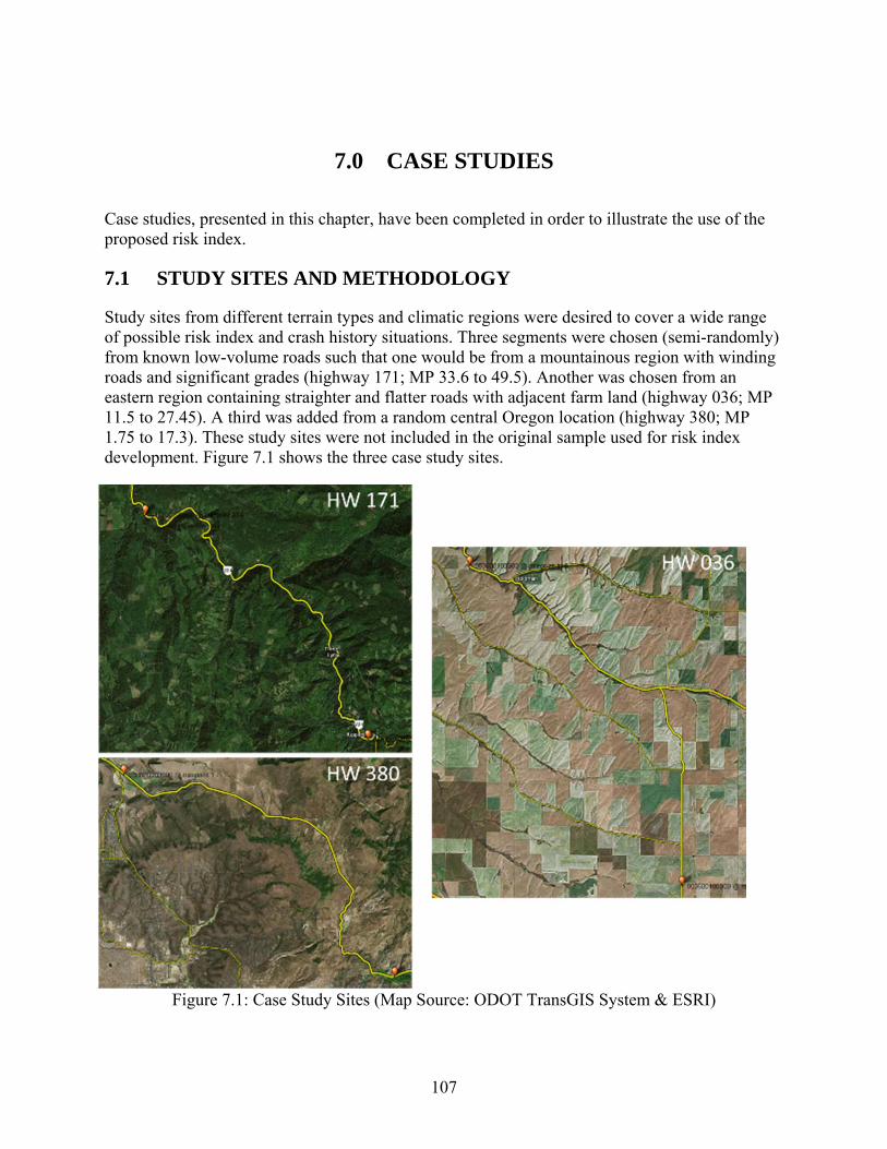
107

7.0 CASE STUDIES

Case studies, presented in this chapter, have been completed in order to illustrate the use of the proposed risk index.

7.1 STUDY SITES AND METHODOLOGY

Study sites from different terrain types and climatic regions were desired to cover a wide range of possible risk index and crash history situations. Three segments were chosen (semi-randomly) from known low-volume roads such that one would be from a mountainous region with winding roads and significant grades (highway 171; MP 33.6 to 49.5). Another was chosen from an eastern region containing straighter and flatter roads with adjacent farm land (highway 036; MP 11.5 to 27.45). A third was added from a random central Oregon location (highway 380; MP 1.75 to 17.3). These study sites were not included in the original sample used for risk index development. Figure 7.1 shows the three case study sites.

Figure 7.1: Case Study Sites (Map Source: ODOT TransGIS System & ESRI)

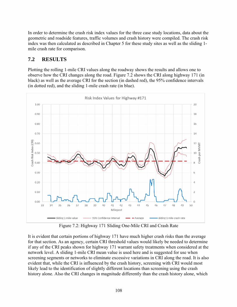
108

In order to determine the crash risk index values for the three case study locations, data about the geometric and roadside features, traffic volumes and crash history were compiled. The crash risk index was then calculated as described in Chapter 5 for these study sites as well as the sliding 1-mile crash rate for comparison.

7.2 RESULTS

Plotting the rolling 1-mile CRI values along the roadway shows the results and allows one to observe how the CRI changes along the road. Figure 7.2 shows the CRI along highway 171 (in black) as well as the average CRI for the section (in dashed red), the 95% confidence intervals (in dotted red), and the sliding 1-mile crash rate (in blue).

Figure 7.2: Highway 171 Sliding One-Mile CRI and Crash Rate It is evident that certain portions of highway 171 have much higher crash risks than the average for that section. As an agency, certain CRI threshold values would likely be needed to determine if any of the CRI peaks shown for highway 171 warrant safety treatments when considered at the network level. A sliding 1-mile CRI mean value is used here and is suggested for use when screening segments or networks to eliminate excessive variations in CRI along the road. It is also evident that, while the CRI is influenced by the crash history, screening with CRI would most likely lead to the identification of slightly different locations than screening using the crash history alone. Also the CRI changes in magnitude differently than the crash history alone, which

109

is expected given that crash history is only one component contributing to the CRI value. For example, while crash rate at MP 43 is notably higher than that at MP 40.8 and MP 37, the CRI at the latter site is the highest among the three sites, which confirms the fact that the use of CRI provide new information about the level of hazard along highway segments compared to using crash history alone.

Figure 7.3 shows the sliding one-mile CRI and crash rate along highway 036.

Figure 7.3: Highway 036 Sliding One-Mile CRI and Crash Rate A quick examination of this figure shows that the third peak in crash rate which occurs at MP 15.8 correspond to a CRI value that is hardly above the average. This suggests that while this location may well belong to the list of sites needing more attention using the crash history alone, it is very unlikely to be identified as such using the CRI value.

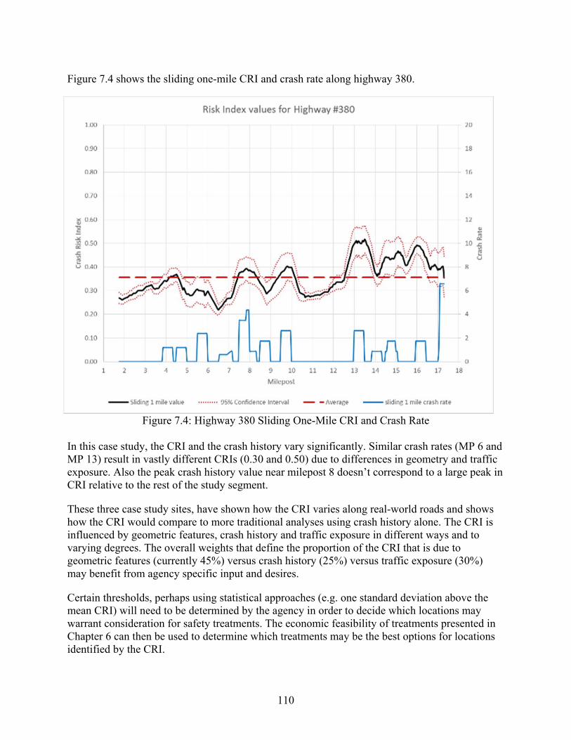
110

Figure 7.4 shows the sliding one-mile CRI and crash rate along highway 380.

Figure 7.4: Highway 380 Sliding One-Mile CRI and Crash Rate In this case study, the CRI and the crash history vary significantly. Similar crash rates (MP 6 and MP 13) result in vastly different CRIs (0.30 and 0.50) due to differences in geometry and traffic exposure. Also the peak crash history value near milepost 8 doesn’t correspond to a large peak in CRI relative to the rest of the study segment.

These three case study sites, have shown how the CRI varies along real-world roads and shows how the CRI would compare to more traditional analyses using crash history alone. The CRI is influenced by geometric features, crash history and traffic exposure in different ways and to varying degrees. The overall weights that define the proportion of the CRI that is due to geometric features (currently 45%) versus crash history (25%) versus traffic exposure (30%) may benefit from agency specific input and desires.

Certain thresholds, perhaps using statistical approaches (e.g. one standard deviation above the mean CRI) will need to be determined by the agency in order to decide which locations may warrant consideration for safety treatments. The economic feasibility of treatments presented in Chapter 6 can then be used to determine which treatments may be the best options for locations identified by the CRI.

111

8.0 SUMMARY

There is a need to better understand the different risks associated with factors and features along low-volume roads. In understanding where risks are present in the system, a proactive approach may be employed to make improvements that can translate into reduced (or prevented) crashes in the future. Overall, six main tasks were completed to address this need.

First a literature review was conducted that sought to identify what factors and features have been identified in past work as presenting a risk to drivers as well as what prospective countermeasures exist to address them. Additionally, this literature review identified and summarized existing approaches to developing risk or safety indices that can be used in identifying where current features pose a potential risk to drivers.

A review of roadside, cross section and alignment features found that several have been identified through past research as posing varying risks to drivers including:



Lane width

Shoulder width

Pavement edge drop-off

Sight distance

Signage and marking

o Speed limit

o Passing zone presence / frequency

o Signage adequacy

o Pavement marking condition

Land use


Driveway density

112

Horizontal curves

Vertical curves

Based on this list, a review of the various countermeasures available to address the various safety issues associated with each feature was also completed. Finally, different approaches were reviewed and summarized that have been developed to establish risk or safety indices. The findings from the literature review provided a basis for understanding which road characteristics may influence crash risk on Oregon’s low-volume roads. These risk influencing features were then investigated along with other potential factors not cited in the literature during the data collection and analysis tasks.

The data collection process was extensive and included gathering road geometry data, roadside feature data, 10-year crash history, and 10-year traffic data for approximately 830 miles of Oregon’s low-volume roads at 0.05 mile resolution. These data were then used in the data analysis task to quantify their effects on crash risk.

The data analysis task completed a number of analyses including overall descriptive statistics of the sample roads and crash characteristics, crash rate analyses leading to a quantification of the effects of individual features on crash risk, and multivariate regression and correlation analyses all of which helped define the crash risk index. The features effecting crash risk and the weights associated with each feature were quantified based on results of the crash analyses.

The crash risk index development task defined an index based on the extensive data analysis efforts. The crash risk index is a function of the geometry of the road and roadside features, crash history, and traffic exposure. The crash risk index quantifies the crash risk and expresses it as a value from 0.15 to 1.0 with higher values corresponding to greater crash risk. The weights of the individual geometric features are based on data analysis and are not recommended for alteration, however, the overall weights that define the proportion of the CRI that is due to geometric features versus crash history versus traffic exposure may benefit from agency specific input.

An economic analysis of potential low-cost safety countermeasures was also completed. The analysis of the proposed safety measures for the low-volume rural road sample has shown certain treatments to be potentially economically beneficial and feasible for implementation. Based on the cost and benefit data gathered and considering the low traffic volumes for these types of roads, the most economically beneficial safety treatments for the low-volume road sample were found to be:





113

Install Safety Edge





Stabilize Shoulders


Widen Un-Paved Shoulder

Flatten Side Slopes



Horizontal Alignment Signs with Static Advisory Speed



The results of the economic analysis are highly depended upon the costs of the treatments. While all efforts were made to choose accurate treatment costs, again agency and region specific cost information could improve the localized benefit / cost ratio results that generated these recommended low-volume treatments.

Lastly, three case studies were completed to illustrate the use of the crash risk index on real world roads in Oregon. Overall, this effort provides a quantification and guidance for improving the safety of low-volume roads.

114

9.0 REFERENCES

Abdel-Rahim, A., and M. Khan. Potential Crash Reduction Benefits of Safety Improvement Projects – Part A: Shoulder Rumble Strips. Report No. FHWA-ID-12-191A. National Institute for Advanced Transportation Technology, 2012. Al-Masaeid, H., and K. Sinha. Analysis of Accident Reduction Potentials of Pavement Markings. Journal of Transportation Engineering. Vol. 120, No. 5, 1994. pp. 723-736 American Traffic Safety Services Association. (ATSSA). Low Cost Local Road Safety Solutions. American Traffic Safety Services Association, Fredericksburg, VA, 2006. American Association of State Highway and Transportation Officials. (AASHTO). Highway Safety Manual First Edition. AASHTO, Washington, D.C., 2010. Arnold, E., and K. Lantz. Evaluation of Best Practices in Traffic Operations and Safety: Phase I: Flashing LED Stop Sign and Optical Speed Bars. Publication FHWA/VTRC 07-R34. FHWA, U.S. Department of Transportation, Federal Highway Administration, Washington, D.C., 2007. Atkinson, J., B. Chandler, V. Betkey, K. Weiss, K. Dixon, A. Giragosian, K. Donoughe, and C. O’Donnell. Manual for Selecting Safety Improvements on High Risk Rural Roads. Report FHWA-SA-14-075. U.S. Department of Transportation, Federal Highway Administration, Washington, D.C. 2014. Austroads. Effectiveness of Road Safety Engineering Treatments. Austroads, Publication No. AP-R422-12, 2012. Austroads. Road Safety Engineering Risk Assessment Part 6: Crash Reduction Factors. Austroads, Publication No. AP-T151/10. 2010. Bahar, G., Mollett, C., Persaud, B., Lyon, C., Smiley, A., Smahel, T., and McGee, H. Safety Evaluation of Permanent Raised Pavement Markers. NCHRP Report 518. National Cooperative Highway Research Program, Transportation Research Board, National Research Council, Washington, D.C. 2004. Balde, A., and S. Dissanayake. Effectiveness of Optical Speed Bars in Reducing Approach Speeds to Rural Communities. Transportation Research Board Annual Meeting, 2011. Bauer, K., and D. Harwood. Safety Effects of Horizontal Curve and Grade Combinations on Rural Two-Lane Roads. Proceedings of the 92nd Annual Transportation Research Record Meeting, 2013.

115

Bendigeri, V., J. Ogle, J. Dillon, and W. Sarasua. Analysis of Factors Contributing to Roadside Tree Crashes in South Carolina Using Laser Data Collection Technologies. Proceedings of the 90th Annual Transportation Research Record Meeting, 2011. Cafiso, S., G. LaCava, and A. Montella. Safety Index for Evaluation of Two-Lane Rural Highways. In Transportation Research Record: Journal of the Transportation Research Board, No. 2019, Transportation Research Board, National Research Council, Washington, D.C., 2007, pp. 136-145. Cafiso, S., A. Di Grazino, G. La Cava, and G. Pappalardo. Cost-Effectiveness Evaluation of Different Safety Intervention Strategies on Two-Lane Rural Highways. Proceedings of the 4th International Symposium on Highway Geometric Design, Valencia, Spain, 2010. Cafiso, S., G. La Cava, and A. Montella. Safety Inspections as Supporting Tool for Safety Management of Low Volume Roads. In Transportation Research Record: Journal of the Transportation Research Board, No. 2203, Transportation Research Board, National Research Council, Washington, D.C., 2011, pp. 116-125. Chen, H., F. Chen, and C. Anderson. Developing an Intelligent Decision Support System for the Proactive Implementation of Traffic Safety Strategies. Report CTS 13-12, Center for Transportation Studies, University of Minnesota, Minneapolis, MN, 2013. Datta, T., T. Gates, and P. Savolainen. Impacts of Non-Freeway Rumble Strips Phase 1. Publication RC-1575. Michigan Department of Transportation, 2012. Davis, P.G. FDOT State Estimates Engineer, Correspondence. May, 2015. deLeur, P., and T. Sayed. Development of a Road Safety Risk Index. In Transportation Research Record: Journal of the Transportation Research Board, No. 1784, Transportation Research Board, National Research Council, Washington, D.C., 2002, pp. 33-42. Donnell, E., V. Karwa, and S. Sathyanarayanan. Analysis of Effects of Pavement Marking Reflectivity on Traffic Crash Frequency on Highways in North Carolina. In Transportation Research Record: Journal of the Transportation Research Board, No. 2103, Transportation Research Board, National Research Council, Washington, D.C., 2009, pp. 50-60. Elvik, R., T. Vaa, A. Hoye, and M. Sorensen. The Handbook of Road Safety Measures. Emerald Group Publishing Limited, Bingley, UK. 2009. Erwin, T. Safety Effects of Preventative Maintenance: Microsurfacing – A Case Study. Thesis for University of Waterloo, Ontario, Canada, 2007. Evans, B., J. Jones, and K. Ksaibati. Implementation of the Wyoming Rural Road Safety Program. Proceedings of the 91st Annual Transportation Research Record Meeting, January, 2012.

116

Federal Highway Administration. (FHWA). Manual on Uniform Traffic Control Devices, ed. Federal Highway Administration, United States Department of Transportation, Washington, D.C., 2009. Accessed at http://mutcd.fhwa.dot.gov/. Accessed February 17, 2014. Federal Highway Administration. (FHWA). Safety Evaluation of the Safety Edge Treatment: Summary Report. Report No. FHWA-HRT-11-025. U.S. Department of Transportation, Federal Highway Administration, 2011. Federal Highway Administration. (FHWA). Technology Partnerships Program to Evaluate LED Raised Pavement Markers. Highways for Life Program: Innovator. FHWA-HIF-12-017, Vol. 5, Issue 28. 2012. Federal Highway Administration. (FHWA). National Road Safety Awards 2013: Noteworthy Practices Guide. U.S. Department of Transportation, Federal Highway Administration, Washington, D.C., 2013. Filcek, M.J., V. Oulevski, J.G. Morena, D.C. Long, and T.L. Maleck. Development of a Profiled Pavement Marking System: Investigation of the Dry/Wet-Night Retroreflectivity and Durability of Pavement Markings Placed in Milled Rumble Strips. Proceedings of the 83rd Annual Transportation Research Record Meeting, 2004. Findley, D., J. Hummer, W. Rasdorf, C. Zegeer, and T. Fowler Modeling the Impact of Spatial Relationships on Horizontal Curve Safety. Accident Analysis and Prevention, Vol. 45, No. 1, 2012, pp. 296-304. Fitzpatrick, K., A. Parham, M. Brewer, and S.-Pin Miaou. Characteristics of and Potential Treatments for Crashes on Low Volume, Rural Tow Lane Highways in Texas. Texas Department of Transportation, Austin, TX, 2001. Fitzpatrick, K., M. Brewer, and A. Parham. Left-Turn and In-Lane Rumble Strip Treatments for Rural Intersections. Publication FHWA/TX-04/0-4278-2. Federal Highway Administration, U.S. Department of Transportation, 2003. Gan, A., P. Shen, and A. Rodriguez. Update of Florida Crash Reduction Factors and Countermeasures to Improve the Development of District Safety Improvement Projects. Lehman Center for Transportation Research – Florida International University, Miami, FL, 2005. Garber, N., and E. Kassebaum. Evaluation of Crash Rates and Causal Factors for High-Risk Locations on Rural and Urban Tow-Lane Highways in Virginia. Report FHWA/VTRC 09-R1, Virginia Department of Transportation, Richmond, 2008. Graham, J., K. Richard, M. O’Laughlin, and D. Harwood. Safety Evaluation of the Safety Edge Treatment. Summary Report FHWA-HRT-11-025. Federal Highway Administration, McLean, VA, 2011.

117

Gregoriades, A., and K. Mouskos. Black Spots Identification Through a Bayesian Networks Quantification of Accident Risk Index. Transportation Research Part C, Vol. 28, 2013, pp. 28-43. Gross, F., K. Eccles, and D. Nabors. Low-Volume Roads and Road Safety Audits - Lessons Learned. In Transportation Research Record: Journal of the Transportation Research Board, No. 2213, Transportation Research Board of the National Research Council, Washington, D.C., 2011, pp. 37-45. Gross, F., and P. Jovanis. Estimation of the Safety Effectiveness of Lane and Shoulder Width: Case-Control Approach. Journal of Transportation Engineering, Vol. 133, No. 6, 2007, pp. 362-369. Gross, F., R. Jagannathan, C. Lyon, and K. Eccles. Safety Effectiveness of “Stop Ahead” Pavement Markings. In Transportation Research Record: Journal of the Transportation Research Board, No. 2056, Transportation Research Board, National Research Council, Washington, D.C., 2008, pp. 25-33. Habibian, M., M. Mesbah, and A. Sobhani. Ranking of Hazardous Road Locations in Two-Lane Two-Way Rural Roads with No Crash Record. Proceedings of the Australasian Transport Research Forum, Adelaide, Australia, 2011. Hallmark, S., E. Peterson, E. Fitzsimmons, N. Hawkins, J. Resler, and T. Welch. Evaluation of Gateway and Low-Cost Traffic-Calming Treatments for Major Routes in Small Rural Communities. Center for Transportation Research and Education, Iowa State University, Ames, IA, 2007. Hallmark, S., T. McDonald, Y. Tian, and D. Andersen. Safety Benefits of Paved Shoulders. Center for Transportation Research and Education – Iowa State University, 2010 Hallmark, S., T. McDonald, and B. Sperry. Evaluation of the Safety Edge in Iowa: Phase II. Center for Transportation Research and Education. 2012 Hallmark, S., N. Hawkins, and O. Smadi. Toolbox of Countermeasures for Rural Two-Lane Curves. Center for Transportation Research and Education – Iowa State University, Ames, IA, 2013a. Hallmark, S., N. Hawkins, and O. Smadi. Evaluation of DSFS and Low Cost Treatments to Reduce Speed and Crashes on Rural Curves. Presentation given at the National Association of County Engineers Conference, 2013b. Hallmark, S., Y. Qiu, M. Pawlovich, and T. McDonald. Assessing the Safety Impacts of Paved Shoulders. Journal of Transportation Safety and Security. Vol. 5, 2013c. pp. 131-147. Hallmark, S., S. Knickerbocker, and N. Hawkins. Evaluation of Low Cost Traffic Calming for Rural Communities – Phase II. Center for Transportation Research and Education. 2013d.

118

Harder, K., J. Bloomfield, and B. Chihak. Stopping Behavior at Real-World Stop-Controlled Intersections with and without In-Lane Rumble Strips. Publication MN/RC-2006-42, Minnesota Department of Transportation, 2006. Harwood, D., F. Council, E. Hauer, W. Hughes, and A. Vogt. Prediction of the Expected Safety Performance of Rural Two-Lane Highways. Report FHWA-RD-99-207. FHWA, U.S. Department of Transportation, Washington, D.C., 2000. Institute of Transportation Engineers. Toolbox of Countermeasures and Their Potential Effectiveness for Intersection Crashes. 2007. Isebrands, H. Rural Road Safety, Systemic Safety with Low Cost Safety Improvements. Presentation to the Wisconsin County Highway Association, 2013. Isebrands, H., S. Hallmark, W. Li, T. McDonald, R. Storm, and H. Preston. Roadway Lighting Shows Safety Benefits at Rural Intersections. Journal of Transportation Engineering, No. 136, 2010. pp. 949-955 Ivan, J., R. Pasupath, and P. Ossenbruggen. Differences in Causality Factors for Single and Multi-vehicle Crashes on Two-lane Roads. Accident Analysis and Prevention, Vol. 31, No. 6, 1999, pp. 695-704. Jiang, Y. The Effectiveness and Criteria for Placement of Raised Pavement Markers - Synthesis Study. Report FHWA/IN/JTRP-2006/6, Indiana Department of Transportation. Indianapolis, IN, 2006. Julian, F., and S. Moler. Gaining Friction in Roadway Safety. FHWA Public Roads, Vol. 72, No. 1, 2008. Jurewicz, C., and R. Troutbeck. A Safe System-based Approach to Selection of Clear Zones, Safety Barriers and Other Roadside Treatments. Proceedings of the Australasian Road Safety Research, Policing and Education Conference, Wellington, New Zealand, 2012. Kirk, A. Evaluation of the Effectiveness of Pavement Rumble Strips. Kentucky Transportation Center. 2008. Knapp, K., and F. Robinson. The Vehicle Speed Impacts of a Dynamic Horizontal Curve Warning Sign on Low-Volume Local Roadways. Report No. CTS 12-12, Minnesota Department of Transportation, St. Paul, MN, 2012. Labi, S. Efficacies of Roadway Safety Improvements across Functional Subclasses of Rural Two-Lane Highways. Journal of Safety Research, No. 42, 2011, pp. 231-239. Latoski, P. Optical Speed Zone for Rural Two-Lane Highways. ITE Journal. 2009.

119

Lord, D., M. Brewer, K. Fitzpatrick, R. Srinivas, and Y. Peng. Analysis of Roadway Departure Crashes on Two-Lane Rural Roads in Texas. Report No. FHWA/TX-11/0-6031-1, Texas Transportation Institute, College Station, TX, 2011. Lyon, C. and Persaud, B. Safety Effects of Targeted Program to Improve Skid Resistance. In Transportation Research Record: Journal of the Transportation Research Board, No. 2068, Transportation Research Board, National Research Council, Washington, D.C., 2008, pp. 135-140. Mahgoub, H., A. Selim, and K.C. Pramod. Quantitative Assessment of Local Rural Road Safety – Case Study. Proceedings of the 90th Annual Transportation Research Record Meeting, 2011. Mahoney, K., R. Porter, E. Donnell, and M. Pietrucha. Evaluation of Centerline Rumble Strips on Lateral Vehicle Placement and Speed on Two-Lane Highways. Pennsylvania Transportation Institute, 2003. Martindale, A., and C. Urlich. Effectiveness of Transverse Road Markings on Reducing Vehicle Speeds. New Zealand Transport Agency, 2010. Massachusetts Traffic Safety Toolbox Series: Pavement Markings. 2008. Matirnez, A., D. Mantaras, and P. Luque. Reducing Posted Speed and Perceptual Countermeasures to Improve Safety in Road Stretches with a High Concentration of Accidents. Safety Science, Vol. 60, 2013, pp. 160-168. McDaniel D., TxDOT Safety Engineer, Correspondence. May, 2015. McGee, H., and F. Hanscom. Low-Cost Treatments for Horizontal Curve Safety. Report No. FHWA-SA-07-002. U.S. Department of Transportation, Federal Highway Administration, Washington, D.C., 2006. McLean, J., G. Veith, and B. Turner. Road Safety Engineering Risk Assessment Part 1: Relationships Between Crash Risk and the Standards of Geometric Design Elements. Report No. AP-T146/10, Austroads, Sydney, New South Wales, 2010. McDonald, T., and R. Sperry. Evaluation of Mitigation for Safety Concerns on Low-Volume, Unpaved Rural Roads. Institute for Transportation, Iowa State University, Ames, IA, 2013. Monsere, C. Preliminary Evaluation of the Safety Effectiveness of Centerline (Median) Rumble Strips in Oregon. Presented at the ITE Quad Conference, Seattle, WA, 2002. Montella, A. Safety Reviews of Existing Roads – Quantitative Safety Assessment Methodology. In Transportation Research Record: Journal of the Transportation Research Board, No. 1922, Transportation Research Board, National Research Council, Washington, D.C., 2005, pp. 62-72.

120

Montella, A. Safety Evaluation of Curve Delineation Improvements: Empirical Bayes Observational Before-and-After Study. In Transportation Research Record: Journal of the Transportation Research Board, No. 2103, Transportation Research Board, National Research Council, Washington, D.C. 2009, pp. 69-79. Montella, A., and F. Mauriello. Procedure for Ranking Unsignalized Rural Intersections for Safety Improvement. In Transportation Research Record: Journal of the Transportation Research Board, No. 2318, Transportation Research Board, National Research Council, Washington, D.C., 2012, pp. 75-82. Moore, A. Evaluation of Experimental Rumble Strips. Research Report No. 186, Louisiana Department of Transportation and Development. 1987. National Cooperative Highway Research Program. (NCHRP) Centerline Rumble Strips. NCHRP Synthesis 339. Transportation Research Board of the National Academies, Washington, D.C., 2005. National Highway Traffic Safety Administration. (NHTSA). Traffic Safety Facts: 2012 Data. USDOT Report DOT HS 812 050. U.S. Department of Transportation, 2014. Neuman, T., R. Pfefer, K. Slack, K. Hardy, F. Council, H. McGee, L. Prothe, and K. Eccles. Guidance for Implementation of the AASHTO Strategic Highway Safety Plan, Volume 6: A Guide for Addressing Run-Off-Road Collisions. NCHRP Report 500. National Cooperative Highway Research Program, Transportation Research Board, National Research Council, Washington, D.C. 2003. Nodari, C., and L. Lindau. Proactive Method for Safety Evaluation of Two-Lane Rural Highway Segments. Proceedings of the 85th Annual Transportation Research Record Meeting, 2006. Olson, D., M. Sujka, and B. Manchas. Performance Analysis of Centerline and Shoulder Rumble Strips Installed in Combination in Washington State. Washington Department of Transportation Research, 2013. Oregon Department of Transportation. (ODOT). Highway Safety Projects Benefit/Cost Analysis Worksheet. (undated). Oregon Department of Transportation. (ODOT). Historical Bid Price Listings by Region, 2014. Pardillo-Mayora, J., C. Dominguez-Lira, and R. Jurado-Pina. Empirical Calibration of a Roadside Hazardousness Index for Spanish Two-Lane Rural Roads. Accident Analysis and Prevention, Vol. 42, No. 6, 2010a, pp. 2018-2023. Pardillo-Mayora, J., C. Domingues-Lira, and R. Jurado-Pina. Calibration of a Roadside Hazardousness Index for Two-Lane Rural Roads. Proceedings of the 89th Annual Transportation Research Record Meeting, 2010b.

121

Park, E., P. Carlson, R. Porter, and C. Andersen. Safety Effects of Wider Edge Lines on Rural, Two-Lane Highways. Accident Analysis and Prevention, Vol. 48, 2012, pp. 317-325. Peng, Y., S.R. Geedipally, and D. Lord. Effect of Roadside Features on Single-Vehicle Roadway Departure Crashes on Rural Two-Lane Roads. In Transportation Research Record: Journal of the Transportation Research Board, No. 2759, Transportation Research Board, National Research Council, Washington, D.C., 2012, pp. 21-29. Persaud, B., R. Retting, and C. Lyon. Crash Reduction Following Installation of Centerline Rumble Strips on Rural Two-Lane Roads. Insurance Institute for Highway Safety, Arlington, VA, 2003. Polus, A., M. Pollatschek, and H. Farah. Input of Infrastructure Characteristics on Road Crashes on Two-Lane Highways. Traffic Injury Prevention, Vol. 6, No. 3, 2005, pp. 240-247. Polus, A., and M. Cohen. Models and Analysis of Accidents on Low-Volume Rural Roads. Proceedings of the 89th Annual Transportation Research Record Meeting, 2010. Potts, I., D. Harwood, C. Bokenkroger, and M. Knoshaug. Benefit/Cost Evaluation of MoDOT’s Total Striping and Delineation Program: Phase II. MRIGlobal. 2011. Prato, C., T. Rasmussen, and S. Kaplan. Risk Factors Associated with Crash Severity on Low-Volume Rural Roads in Denmark. Journal of Transportation Safety and Security, Vol. 6, No. 1, 2014, pp. 1-20. Qin, X., and A. Wellner. Development of Safety Screening Tool for High Risk Rural Roads in South Dakota. South Dakota State University, Brookings, SD, 2011. Schneider, W., P. Savolainen, and K. Zimmerman. Driver Injury Severity Resulting from Single-Vehicle Crashes Along Horizontal Curves on Rural Two-Lane Highways. In Transportation Research Record: Journal of the Transportation Research Board, No. 2102, TRB, National Research Council, Washington, D.C., 2009, pp. 85-92. Schrum, K., K. Lechtenberg, C. Stolle, R. Faller, and D. Sickling. Cost-Effective Safety Treatments for Low-Volume Roads. Report No. TRP-03-222-12, Nebraska Department of Roads, Lincoln, August 2012. Simpson, C., and S. Troy. Evaluation of the Safety Effectiveness of Vehicle Entering When Flashing; Signs and Actuated Flashers at 74 Stop-Controlled Intersections in North Carolina. Proceedings of the 92nd Annual Transportation Research Record Meeting, January, 2013. Simpson, C., and S. Troy. Vehicle Entering When Flashing Evaluation. Presentation October, 2012 at unknown location retrieved from https://connect.ncdot.gov/resources/safety/Safety%20Evaluation%20Completed%20Projects/VEWF%20Presentation_102412.pdf Accessed January, 2014.

122

Souleyrette, R., M. Caputcu, T. McDonald, R. Speery, Z. Hans, and D. Cook. Safety Analysis of Low-Volume Rural Roads in Iowa. Report No. 07-309, Iowa Department of Transportation, Ames, 2010. Sperry, R., J. Latterell, and T. McDonald. Best Practices for Low-Cost Safety Improvements on Iowa’s Local Roads. Report CTRE-08-338. Iowa Department of Transportation, Ames, IA, 2008. Srinivasan, R., J. Baek, D. Carter, B. Persaud, C. Lyon, K. Eccles, F. Gross, and N. Lefler. Safety Evaluation of Improved Curve Delineation. Report No. FHWA-HRT-09-045. U.S. Department of Transportation, Federal Highway Administration, Washington, D.C., 2009. Srinivasan, R., J. Baek, and F. Council. Safety Evaluation of Transverse Rumble Strips on Approaches to Stop-Controlled Intersections in Rural Areas. Journal of Transportation Safety and Security, Vol. 2, 2010, pp. 261-278. Stamatiadis, N., S. Jones, and L. Aultman-Hall. Causal Factors for Accidents on Southeastern Low-Volume Rural Roads. In Transportation Research Record: Journal of the Transportation Research Board, No. 1652, Transportation Research Board, National Research Council, Washington, D.C., 1999, pp. 111-117. Sun, X., J. Park, V. Tekell Jr., and N. Ludington. Evaluation of Pavement Edge Lines on Narrow Highways with Low Traffic Volume in Louisiana. In Transportation Research Record: Journal of the Transportation Research Board, No. 1989, Transportation Research Board, National Research Council, Washington, D.C., 2007, pp. 115-122. Sun, X., and S. Das. Safety Improvements from Edge Lines on Rural Two-Lane Highways. Report No. FHWA/LA.11/487, University of Louisiana at Lafayette. 2012. Thompson, T., M. Burris, and P. Carlson. Speed Changes Due to Transverse Rumble Strips on Approaches to High-Speed Stop-Controlled Intersections. In Transportation Research Record: Journal of the Transportation Research Board, No. 1973, Transportation Research Board of the National Academies, Washington, D.C., 2006, pp. 1-9 Van Schalkwyk, I., and S. Washington. Cost Effective Safety Improvements on Two-Lane Rural State Roads in Washington State. Report WA-RD 695.1, Washington State Department of Transportation, Olympia, WA, 2008. Veneziano, D., N. Villwock-Witte, and A. Al-Kaisy. Cost Effective Local Road Safety Planning and Implementation. American Traffic Safety Services Association, Fredericksburg, VA, 2011. Veneziano, D., and N. Villwock-Witte. Safety Opportunities in High Friction Surfacing. American Traffic Safety Services Association, Fredericksburg, VA, 2013. Vest, A., N. Stamatiadis, A. Clayton, and J. Pigman. Effect of Warning Devices on Curve Operating Speeds. Publication KTC-05-20/SPR-259-03-1F. Kentucky Transportation Cabinet, 2005.

123

Waiby, G.. F. Tate, and C. Brodie. The Development of a Proactive Road Safety Assessment Tool – KiwiRap. Proceedings of the Australasian Road Safety Research, Policing and Education Conference, Wellington, New Zealand, 2012. Wang, C., K. Dixon, and D. Jared. Evaluating Speed Reduction Strategies for Highway Work Zones. In Transportation Research Record: Journal of the Transportation Research Board, No. 1824, Transportation Research Board of the National Academies,Washington, D.C., 2003, pp. 44-53. Wang, C., M. Quddus, and S. Ison. The Effect of Traffic and Road Characteristics on Road Safety: A Review and Future Research Direction. Safety Science, Vol. 57, 2013, pp. 264-275. Wang, Y., N. Ha Nguyen, A. Levy, and Y.-Jau Wu. Cost Effective Safety Improvements for Two-Lane Rural Roads. Report No. TNW 2008-04, University of Washington, Seattle, WA, 2008. White, D., M. Mekkawy, C. Jahren, D. Smith, and M. Suleiman. Effective Shoulder Design and Maintenance. Report IHRB-TR-531 for Iowa Highway Research Board. 2007. Zador, P., P. Wright, and R. Karpf. Effect of Pavement Markers on Nighttime Crashes in Georgia. Insurance Institute for Highway Safety. Washington, D.C., 1982. Zegeer, C., D. Reinfurt, T. Neuman, J. Stewart, and F. Council. Safety Improvements on Horizontal Curves for Two-Lane Rural Roads. Report No. FHWA-RD-90-074. FHWA, U.S. Department of Transportation, Washington, D.C., 1990. Zegeer, C., R. Stewart, F. Council, and D. Reinfurt. Cost Effective Geometric Improvements for Safety Upgrading of Horizontal Curves. Report No. FHWA-RD-90-021. FHWA, U.S. Department of Transportation, Washington, D.C., 1991.

APPENDIX A DATA SAMPLE DEFINITION

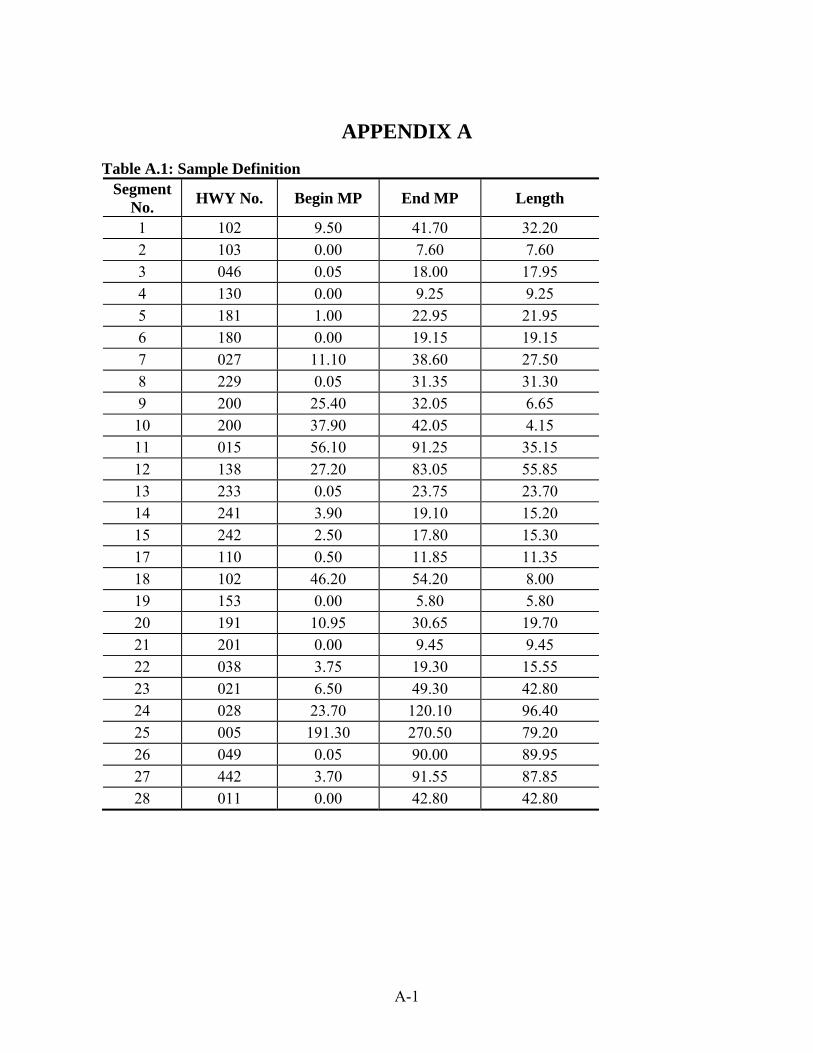
A-1

APPENDIX A

Table A.1: Sample Definition Segment

No. HWY No. Begin MP End MP Length

1 102 9.50 41.70 32.202 103 0.00 7.60 7.603 046 0.05 18.00 17.954 130 0.00 9.25 9.255 181 1.00 22.95 21.956 180 0.00 19.15 19.157 027 11.10 38.60 27.508 229 0.05 31.35 31.309 200 25.40 32.05 6.6510 200 37.90 42.05 4.1511 015 56.10 91.25 35.1512 138 27.20 83.05 55.8513 233 0.05 23.75 23.7014 241 3.90 19.10 15.2015 242 2.50 17.80 15.3017 110 0.50 11.85 11.3518 102 46.20 54.20 8.0019 153 0.00 5.80 5.8020 191 10.95 30.65 19.7021 201 0.00 9.45 9.4522 038 3.75 19.30 15.5523 021 6.50 49.30 42.8024 028 23.70 120.10 96.4025 005 191.30 270.50 79.2026 049 0.05 90.00 89.9527 442 3.70 91.55 87.8528 011 0.00 42.80 42.80

APPENDIX B REGRESSION RESULTS

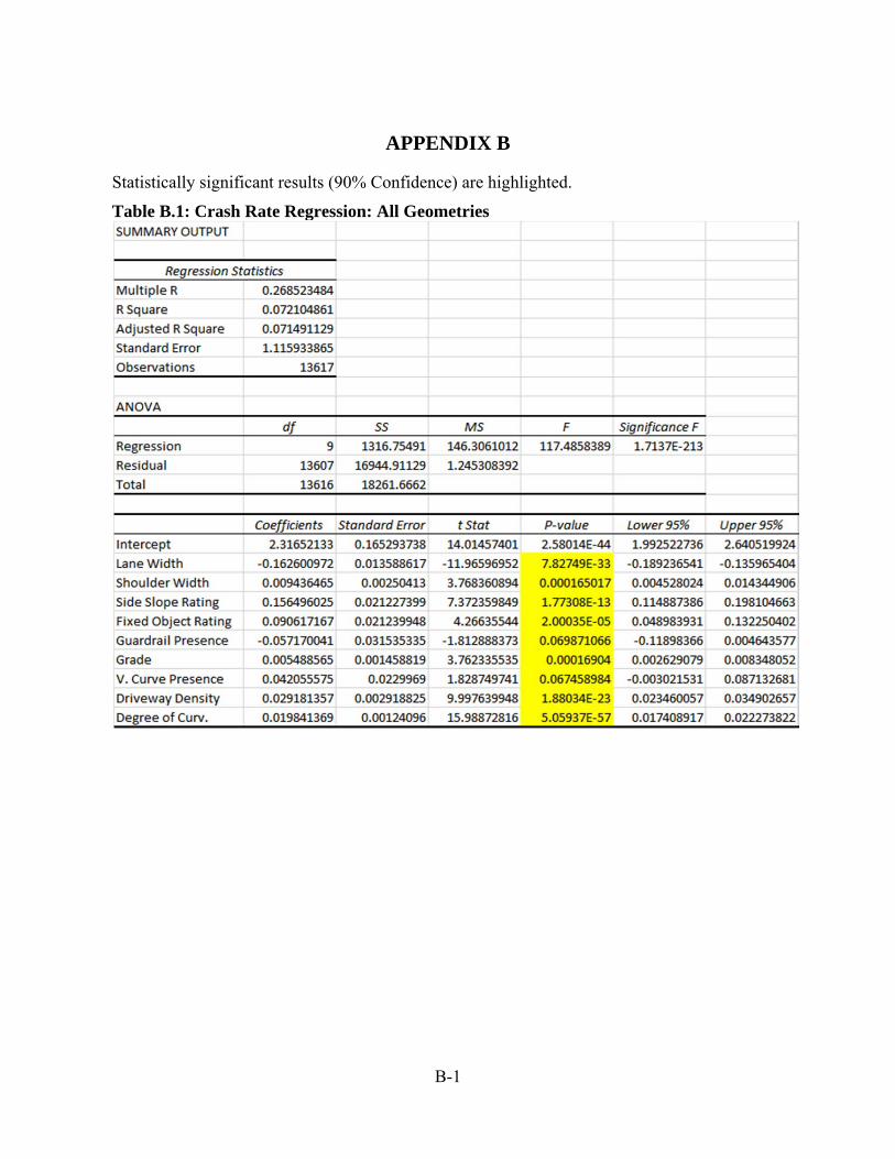
B-1

APPENDIX B

Statistically significant results (90% Confidence) are highlighted.

Table B.1: Crash Rate Regression: All Geometries

B-2

Table B.2: Crash Rate Regression: Tangents

B-3

Table B.3: Crash Rate Regression: Curves

B-4

Table B.4: Crash Severity Rate Regression: All Geometries

B-5

Table B.5: Crash Severity Rate Regression: Tangents

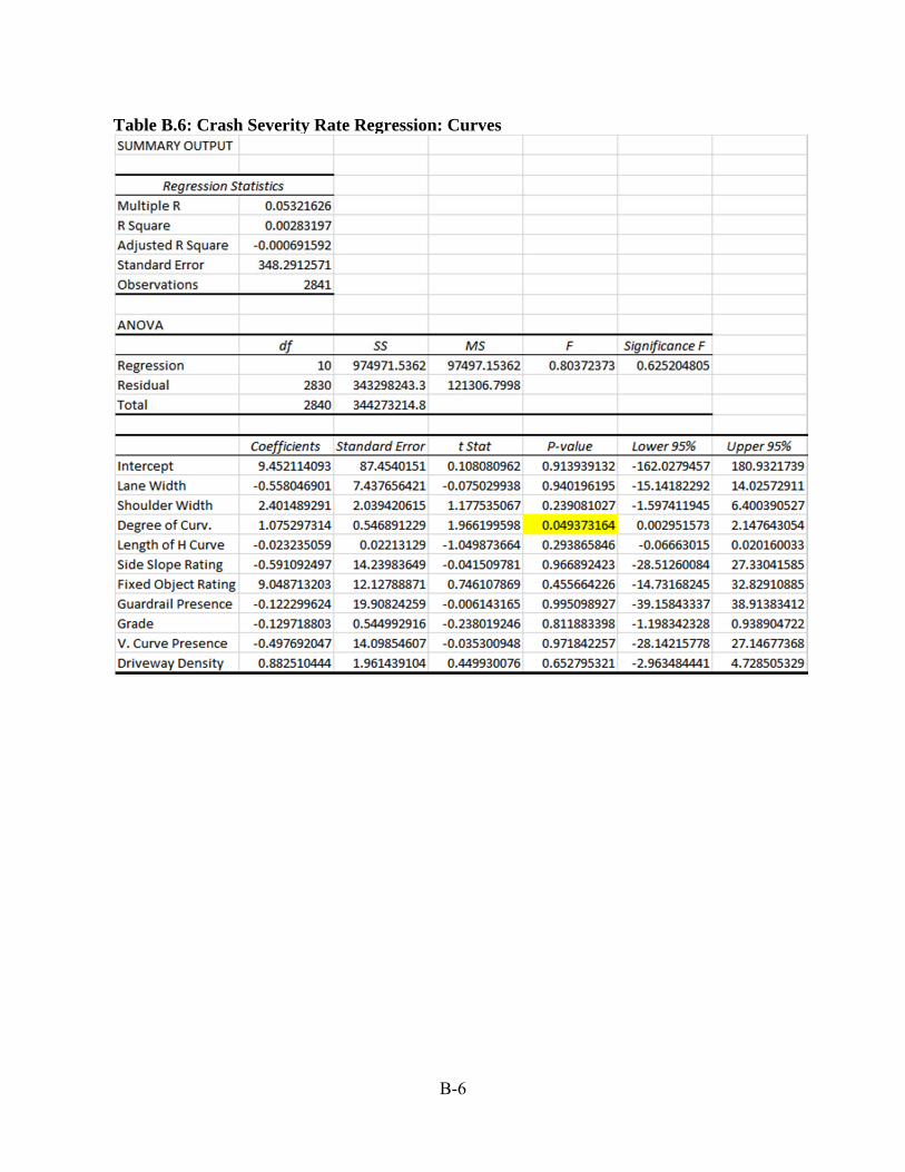
B-6

Table B.6: Crash Severity Rate Regression: Curves

APPENDIX C CORRELATION RESULTS

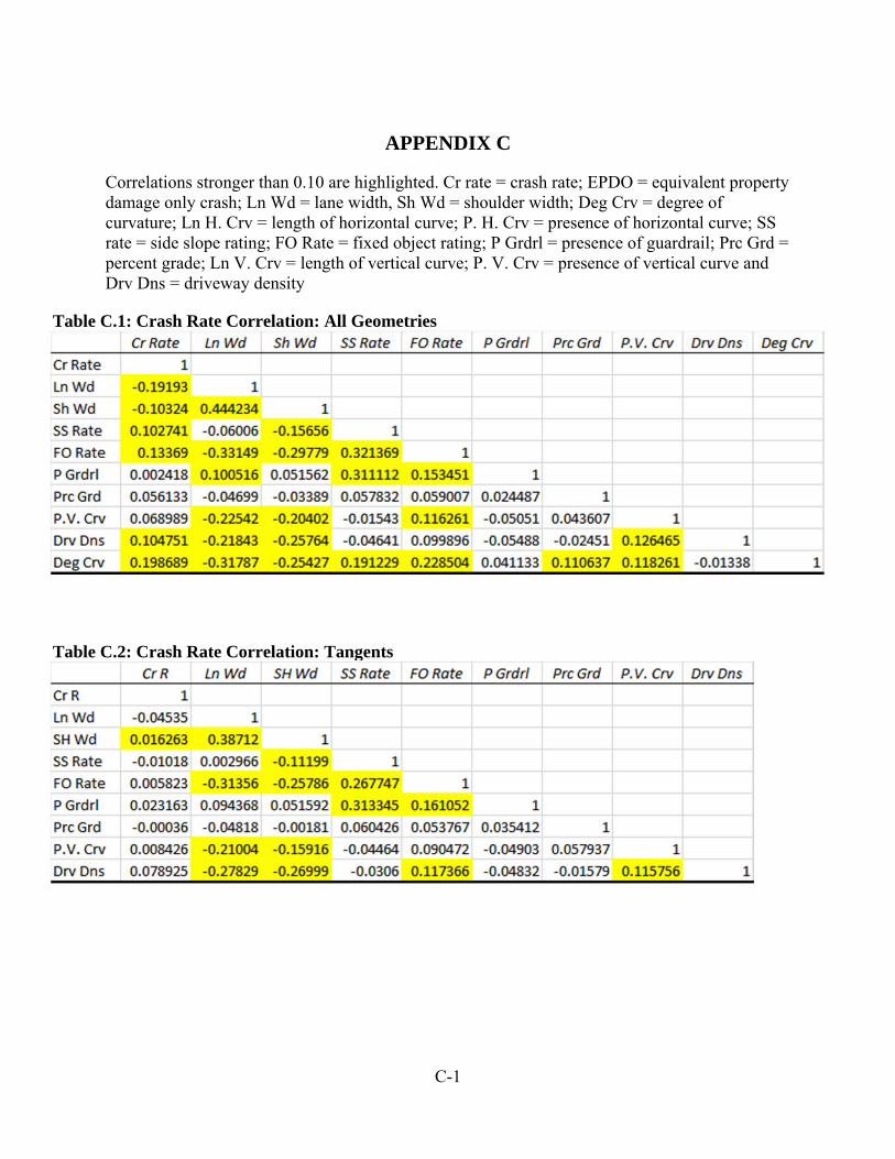
C-1

APPENDIX C

Correlations stronger than 0.10 are highlighted. Cr rate = crash rate; EPDO = equivalent property damage only crash; Ln Wd = lane width, Sh Wd = shoulder width; Deg Crv = degree of curvature; Ln H. Crv = length of horizontal curve; P. H. Crv = presence of horizontal curve; SS rate = side slope rating; FO Rate = fixed object rating; P Grdrl = presence of guardrail; Prc Grd = percent grade; Ln V. Crv = length of vertical curve; P. V. Crv = presence of vertical curve and Drv Dns = driveway density

Table C.1: Crash Rate Correlation: All Geometries

Table C.2: Crash Rate Correlation: Tangents

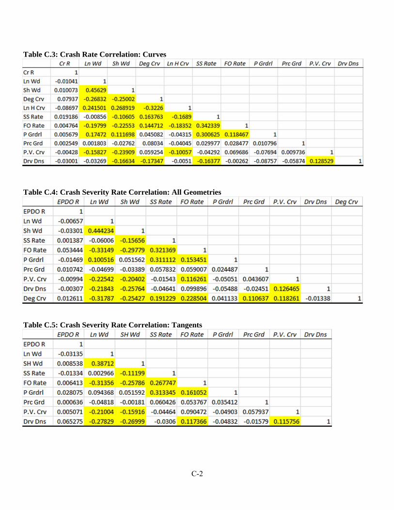
C-2

Table C.3: Crash Rate Correlation: Curves

Table C.4: Crash Severity Rate Correlation: All Geometries

Table C.5: Crash Severity Rate Correlation: Tangents

C-3

Table C.6: Crash Severity Rate Correlation: Curves

APPENDIX DGEOMETRIC FEATURE PLOTS

D-1

APPENDIX D

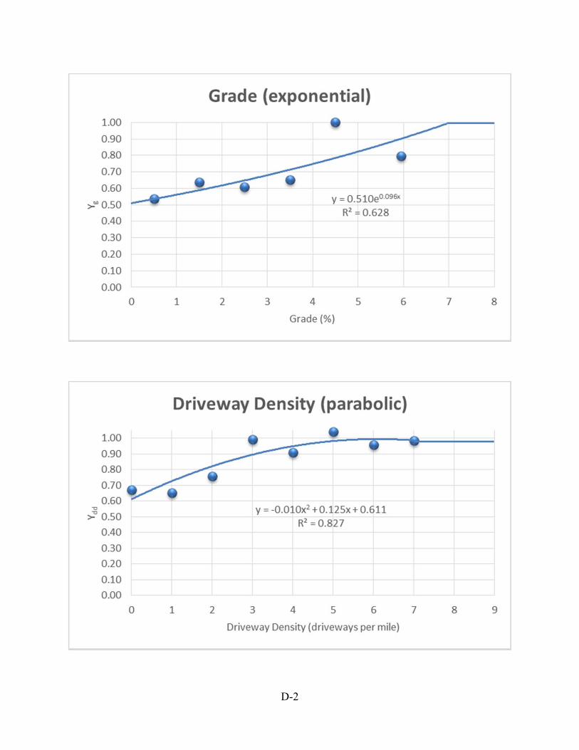
D-2

D-3

D-4

APPENDIX EBENEFIT-COST SAMPLE CALCULATION

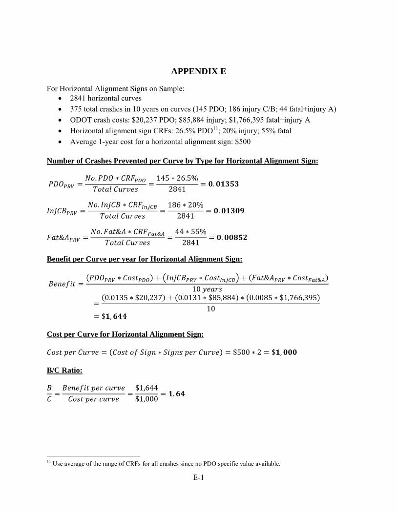
E-1

APPENDIX E

For Horizontal Alignment Signs on Sample: 2841 horizontal curves

375 total crashes in 10 years on curves (145 PDO; 186 injury C/B; 44 fatal+injury A)

ODOT crash costs: $20,237 PDO; $85,884 injury; $1,766,395 fatal+injury A

Horizontal alignment sign CRFs: 26.5% PDO11; 20% injury; 55% fatal

Average 1-year cost for a horizontal alignment sign: $500

Number of Crashes Prevented per Curve by Type for Horizontal Alignment Sign:

. ∗

145 ∗ 26.5%

2841.

. ∗

186 ∗ 20%2841

.

&. & ∗ &

44 ∗ 55%2841

.

Benefit per Curve per year for Horizontal Alignment Sign:

∗ ∗ & ∗ &

100.0135 ∗ $20,237 0.0131 ∗ $85,884 ∗ 0.0085 ∗ $1,766,395

10$ ,

Cost per Curve for Horizontal Alignment Sign:

∗ $500 ∗ 2 $ ,

B/C Ratio:

$1,644$1,000

.

11 Use average of the range of CRFs for all crashes since no PDO specific value available.

Documents

RISK FACTORS ASSOCIATED WITH HIGH … FACTORS ASSOCIATED WITH HIGH POTENTIAL FOR SERIOUS CRASHES Final ... Risk Factors Associated with High Potential for Serious ... (Veneziano …