Risk management based on GARCH and Non …239419/FULLTEXT01.pdfGARCH and Non-parametric stochastic volatility models and some cases of Generalized Hyperbolic distribution ... in every

Technical report, IDE0832 , October 29, 2008

Risk management based onGARCH and Non-parametricstochastic volatility models

and some cases of GeneralizedHyperbolic distribution

Master’s Thesis in Financial Mathematics

Askerbi Midov and Konstantin Balashov

School of Information Science, Computer and Electrical EngineeringHalmstad University

Risk management based on GARCHand Non-parametric stochastic

volatility models and some cases ofGeneralized Hyperbolic distribution

Askerbi Midov and Konstantin Balashov

Halmstad University

Project Report IDE0832

Master’s thesis in Financial Mathematics, 15 ECTS credits

Supervisors: Prof. Albert N. Shiryaev, Ph.D. Jan-Olof JohanssonExaminer: Prof. Ljudmila A. Bordag

External referee: Prof. Lioudmila Vostrikova

October 29, 2008

Department of Mathematics, Physics and Electrical EngineeringSchool of Information Science, Computer and Electrical Engineering

Halmstad University

Acknowledgements

We would like to thank Albert Nikolaevich Shiryaev for useful hints in thedirection of the research and Jan-Olof Johansson who supported the projectin every day work, discussed with us our problems and gave us plenty ofideas. Special thanks to Ljudmila Bordag for her attention to our life duringthe time in Halmstad and lots of helpful advices.

ii

Abstract

The paper is devoted to the modern methods of Value-at-Risk calcu-lation using different cases of Generalized Hyperbolic distribution andmodels for predicting volatility. In our research we use GARCH-M andNon-parametric volatility models and compare Value-at-Risk calcula-tion depending on the distribution that is used. In the case of Non-parametric model corresponding windows are proved by the Cross Val-idation method. Furthermore in our work we consider adaption of themethod to intraday data using ACD and UHF-GARCH models. Theproject involves also application of the developed methods to real finan-cial data and comparable analysis of the obtained results.

iii

iv

Contents

1 Introduction 1

2 Models description 52.1 General model . . . . . . . . . . . . . . . . . . . . . . . . . . . 52.2 Stochastic volatility . . . . . . . . . . . . . . . . . . . . . . . . 62.3 Levy processes . . . . . . . . . . . . . . . . . . . . . . . . . . . 102.4 Risk management . . . . . . . . . . . . . . . . . . . . . . . . . 14

3 Methods 173.1 Volatility estimation . . . . . . . . . . . . . . . . . . . . . . . 173.2 The driving Generalized Hyperbolic process estimation . . . . 213.3 Value-at-Risk calculation . . . . . . . . . . . . . . . . . . . . . 22

4 Backtestings and conclusions 23

Appendix 39

Bibliography 59

v

vi

Chapter 1

Introduction

Nowadays risk is an essential part of the financial world. Estimation of themarket risk is one of the main problems that different types of financial in-stitutions face every day. This kind of risk arises because of fluctuations ofinterest rates, commodity prices, stock prices, exchange rates etc. As thereis direct relation between these movements and investor’s gains or losses, weget the necessity to estimate the market risk as precise as possible. Thereexist a lot of different risk measures. But most of them do not provide exactinformation about magnitude of losses. For example if we consider one ofthe most well-known risk-measures standard deviation (volatility), we obtaininformation just about the magnitude of changes in price, but not about theamount of possible losses. Therefore today such instrument as Value-at-riskbecame one of the most preferable methods to quantify risk on financial mar-kets. In the present financial world VaR, a quantile measure, has become themost widespread approach to estimate the market risk and for the last sev-eral years it has been a really popular and useful tool in risk management.But VaR measure had been known for quite a long time before it came intouse in financial lexicon. In 1952 Harry Markowitz[22] used VaR in his paper”Portfolio selection” to evolve methods of portfolio optimization. Later sincemiddle 1980s till 1990s a lot of financial institutions adopted VaR measureto deal with capital allocation and market risk. In 1994 J.P. Morgan, one ofthe biggest investment companies of the United States released it’s free riskmanagement service Risk Metrics that represented VaR as a basic approachfor market risk estimation. Even now values that are obtained using thisservice are considered to be a kind of a standard of VaR calculation. Finallyin 1995 the Basel Committee on Banking Supervision set requirements con-cerning market risk capital reserves based on VaR measure. After all thesestages of development this approach has become one of the main methodsfor estimating market risk.

1

2 Chapter 1. Introduction

There exist three main approaches for VaR calculation: historical, variance-covariance and Monte-Carlo Simulations. The main aim of this research is toinvestigate variance-covariance method and to introduce some improvementsby using non-normal density functions.In general VaR is a probabilistic measure that gives us opportunity to mea-sure the risk of a portfolio or a single asset with just one number that ac-cumulates all the information about the risk that is taken. To computeValue-at-Risk we need to have some model for describing price behavior. Inthis work we use a model that is based on two main components: StochasticVolatility and Levy processes. Such model was investigated in the paper ofEberlein, Kallsen and Kristen (2003)[10]. The first component, Volatility, isa very important characteristic of the market. To estimate the market risksufficiently precise one should take it into account. In contrary of the Black-Scholes approach the idea of the stochastic volatility price model is basedon the empirical fact that volatility is not constant and in the real world itchanges randomly. Stochastic volatility is very well-known and widely usedin financial world. There are a lot of works where it was described and in-vestigated, such as Hull and White (1998)[21], Barone-Adesi et al. (1998,1999)[2], Guermat and Harris (2002)[18], Venter and de Jongh (2002)[26],McNeil and Frey (2000)[23].The second component is Levy processes. More precisely speaking to achieveour goals we will take into consideration some cases of Generalized Hyperbolicdistributions that were introduced in papers of Brandorff-Nielsen (1998)[1],Eberlein (2001)[8], Eberlein and Prause (2002)[9]. These kinds of distribu-tions are much more flexible then normal distribution. That is why they canprovide better fit to empirical data.There are three main goals that should be achieved at the end of the work.The first one is to compare two markets, the comparably small Stockholmand the rather big Frankfurt exchange markets. We will do this by analyzingthe DAX and the OMXS30 indexes correspondingly. We will investigate thebehavior of the volatility on both markets and try to find if they are corre-lated or not. The second goal is to calculate VaR using the same indexesfrom two exchange markets that were mentioned. To do so we will comparedifferent types of generalized hyperbolic distributions to decide which onewill provide the best fit to the empirical data. Also we will compare VaRresults obtained by using different generalized hyperbolic distributions withVaR calculated using Normal Gaussian distribution. And finally the thirdaim of this paper is to apply a model for estimation of volatility using tickdata and conditional duration for VaR calculationThe paper is composed in the next consecution: we will start with presen-tation of Value-at-Risk calculation methods overview. Later in Chapter 1

Risk management based on VaR estimation 3

two basic components, stochastic volatility and generalized hyperbolic dis-tributions, with their partial cases and basic notions are introduced. Furtherin Chapter 2 we describe methods of volatility prediction and estimation ofdistribution parameters for logarithmic returns. At the end of the chapter wewill suggest methods to access the accuracy of calculations. The results thatwere obtained in this research and description of the used data are presentedin Chapter 3. Finally the meaning of these results and ideas for furtherinvestigation are discussed in Conclusion section.

4 Chapter 1. Introduction

Chapter 2

Models description

2.1 General model

Consider the price process of such type St = S0eXt . We suggest to model

log-return process ∆Xt = Xt − Xt−1 as it was done in the paper Eberlein,Kallsen and Kristen (2003)[10]

∆Xt = σt∆Lt (2.1)

where σt is a stochastic volatility series and ∆Lt - white noise.Definition(Wide sense white noise) : The sequence εt is called white noisein the wide sense if Eεt = 0, Eε2t <∞ and

Eεkεm = 0, ∀ k 6= m

In the above mentioned paper Eberlein, Kallsen and Kristen (2003)[10], au-thors argue that such model is rather natural. They considered Dow Jonesindex returns data of very large time period and have found that real resid-uals

log ∆X2t − log σ2

t

look very similar with simulated standard normal white noise. But in fact,during the given comparison very common effects of price were recognized

1. Large positive value of residuals appear much more rarely in the Gaussiansample than for real data. This illustrates the well-known fact that re-turn data has heavier tails than normal distribution.

2. We can observe additionally some clusters of extremely high values.Which tell us that there may be a very short-lived volatility componentin the data.

5

6 Chapter 2. Models description

3. The time series

log ∆X2t = log σ2

t + log ∆L2t

can be considered as a signal log σ2t perturbed by an white noise, which

has a mean E log ∆L21

Due to this observations the suggested general model seems to be very robust.In the paper the authors describe residuals white noise using Hyperbolicdistribution instead of Normal. In our research we consider a wide class -General Hyperbolic distributions, which are tailor-made and flexible enoughfor fitting real data. Let’s take a closer look to the basic components of themodel.

2.2 Stochastic volatility

In modern financial mathematics volatility is considered to be nearly themost investigated phenomenal occurrence because of two reasons. First ofall for the last several years the usage of financial derivatives has increaseddramatically and volatility is involved in their calculation. The second rea-son is directly related with the subject of this paper and consists in thatthe volatility of the stock returns plays the central role in risk managementand particularly in such method as VaR. From the beginning Black-Scholes(1973)[3] the volatility was assumed to be constant but the existence of suchphenomena as the volatility smile showed that it appears to vary indeed.Stochastic volatility models were introduced to obtain the possibility to de-scribe such empirical tendency that exists on financial markets and is nottaken into account by the constant volatility models. The main idea of thestochastic volatility is to present the volatility itself as a stochastic process.Definition(Stochastic volatility) : A process in which the return fluctu-ation includes an unobservable component which cannot be predicted usingcurrent available information .In other words it is a model in which volatility is presented as a randomlychanging process described by a discrete random process or a stochastic dif-ferential equation.In the paper Eberlein, Kallsen and Kristen (2003)[10] introduced an ex-ploratory analysis of stochastic volatility based on the Dow Jones Indus-trial Average index. In that research the authors substantiated the necessityof using stochastic volatility models by performing a qualitative analysis ofvolatility fluctuations and showed that besides the slowly varying stochas-tic volatility there exist really short-period volatility constituents. Also hepractically showed that a widely known fact that the stock returns data have


heavier tails rather than if it was normally distributed really appears to be.We have already mentioned the model for our returns:

∆Xt = σt∆Lt

Where the volatility can be determined as shown below:

• ARCH

σ2t = a0 +

p∑i=1

ai∆X2t−i a0 > 0, ai ≥ 0

From the equation we can see that the volatility is a fully determinis-tic function of previous returns. Also it is necessary to mention thatprevious big returns result in big value of the volatility and small re-turns give us small volatility. This is called Autoregressive ConditionalHeteroscedastic model or ARCH(p). This model was very widely usedbecause it explained such phenomena as heavy tails of return data,clustering etc. that linear stochastic models could not explain (AR,MA, ARMA etc.) cf. Shiryaev (1998)[25].

• GARCHAs a further development there appeared a generalized form of thismodel called GARCH(p, q):

σ2t = a0 +

p∑i=1

ai∆X2t−i +

q∑j=1

biσ2t−i

Here a0 > 0, ai ≥ 0, bi ≥ 0. In this case the volatility depends notonly on the previous values of returns, but also on the previous valuesof the volatility itself. Now let’s consider a particular case of this modelthat we will use for our research called GARCH(1.1)-M. (cf. Shephard(1996)[24], Shiryaev (1998)[25] section II. 3a(10)):

σ2t = a0 + a1σ

2t−1(∆L

2t−1 −m)2 + b1σ

2t−1

Where a0 > 0, a1, b1 ≥ 0, m = E∆L1. This is a really widely usedstochastic volatility model that shows that big values of the volatilityappear because of the large absolute values of previous returns.

• Non− parametricVolatility modeling is possible not just with parametric models. We cansuppose that the volatility is changing according to some arbitrary sto-chastic process but slowly. We assume that the endurance of volatility


changes is longer than the interval of the historical observations. So wecan say that tomorrow volatility is more likely to keep its tendency andin such case we can use a moving average to predict volatility one dayahead. Our goal is to revile volatility signal masked with noise fromthe historical data. To do this we use a non-parametric smoothing (cf.Hardle (1991))[19].

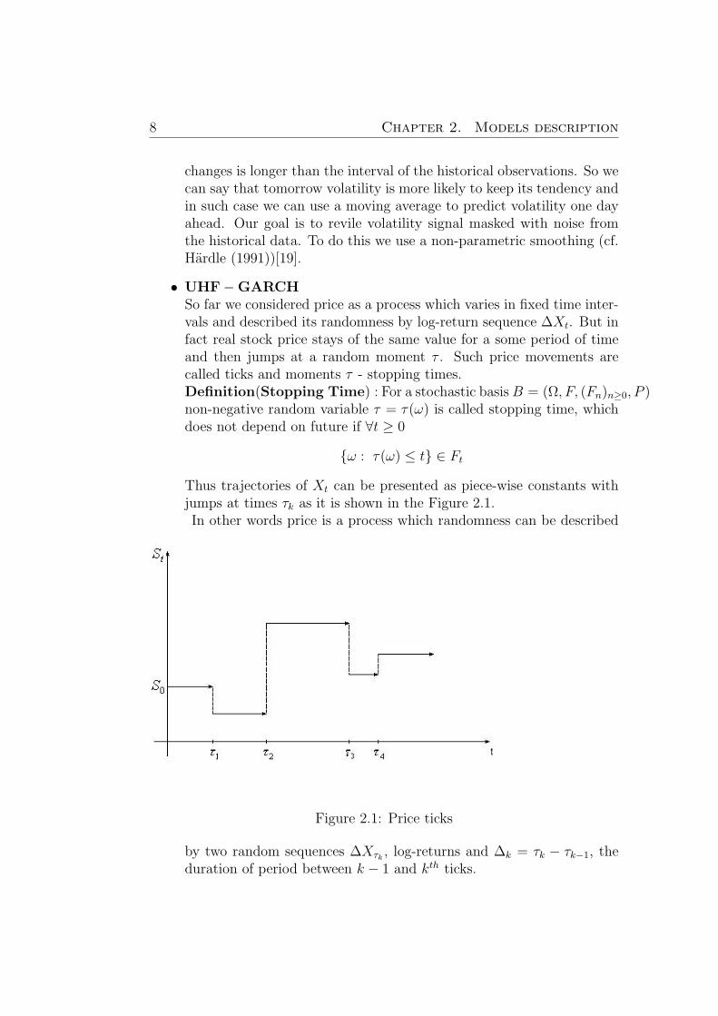
• UHF−GARCHSo far we considered price as a process which varies in fixed time inter-vals and described its randomness by log-return sequence ∆Xt. But infact real stock price stays of the same value for a some period of timeand then jumps at a random moment τ . Such price movements arecalled ticks and moments τ - stopping times.Definition(Stopping Time) : For a stochastic basisB = (Ω, F, (Fn)n≥0, P )non-negative random variable τ = τ(ω) is called stopping time, whichdoes not depend on future if ∀t ≥ 0

ω : τ(ω) ≤ t ∈ Ft

Thus trajectories of Xt can be presented as piece-wise constants withjumps at times τk as it is shown in the Figure 2.1.In other words price is a process which randomness can be described

Figure 2.1: Price ticks

by two random sequences ∆Xτk , log-returns and ∆k = τk − τk−1, theduration of period between k − 1 and kth ticks.


In the above section we discussed how to model log-returns. But thequestion is how to model this random sequence ∆k and it is interestingto receive some past dependence for them, because in reality durationbetween ticks are correlated.For our research we use the model which was investigated in Engle,Russel (1998)[13]. In this model durations assumes to be correlatedand all past dependence is included in function ψ, where ∆

ψ∼ i.i.d..

Also one can realize that process in the Figure 2.1 looks similar withwell-known Poisson process, where the periods of time between ticksare exponentially distributed. It could be transformed for modelingdesirable durations distribution and seems to be a good starting point.Thus first simple case of the model has exponential distribution withparameter λ = 1

ψ. It is called Exponential ACD or just EACD

p(∆k|ψk) =1

ψke−∆kψk

where

ψk = ω +

p∑i=1

αi∆k−i +

q∑j=1

βjψk−j

andψ0 =

ω

1− β

This formula for ψ is very similar with GARCH(p,q) and it is calledAutoregressive Conditional Duration model or ACD(p,q). As in theGARCH it is more convenient to work with ACD(1,1)

ψk = ω + α∆k−1 + βψk−1

The second more general case of the model assumes that conditionaldistribution of durations is Weibull, where (∆k

φk)γ is exponential. It is

called Weibull ACD or just WACD model. The density function thenlooks like that

g(∆k) =γ

∆k

(∆k

φk

)γ

e−

∆kφk

γ∀∆k > 0

whereφk = ω + α∆k−1 + βφk−1

φk =ψk

Γ(1− 1

γ

)


and Γ is a Gamma function. Another reasonable question arises - howcan we use these durations for our risk management purposes?It was noticed in Engle (2000)[14] that there exists some correlationbetween durations of periods when price is a constant and volatility.Indeed, when durations between price ticks a very long, it correspondsto the situation when trading transactions occur very rarely. Accordingto that, the volatility of the price will be very low and vice versa.This fact tell us about negative correlation between these two processes.Define the conditional variance of log-returns per unit of time. Inorder to do that we divide log-returns by the square root of the currentduration

V ar

(∆Xt√

∆t

|∆t

)= σ2

t

Define new sequence∆Xt√

∆t

= εt (2.2)

which is consist of log-returns per unit of time. Then GARCH(1,1)volatility model for such process looks like that

σ2t = ω + αε2t−1 + βσ2

t−1

This model can be applied if we think that current duration does notprovide any information about volatility. Another more interesting caseof the volatility model due to negative correlation effect seems to bemore realistic

σ2t = a+ bε2t−1 + cσ2

t−1 + d∆−1t (2.3)

Usually durations between price movements are very small time inter-vals measured in seconds that is why equation 2.3 is called Ultra-HighFrequency or just UHF-GARCH(1,1). Estimation parameters proce-dure and one-step prediction for duration models will be presented inthe subsequent chapter.As it was shown in Eberlein, Ozkan (2002)[11] in the case when thetime scale is very small, estimations of the white noise ∆Lt with Gen-eralized Hyperbolic distribution is still consistent. Hence we can applyabove defined UHF-GARCH volatility approach to our general model.

2.3 Levy processes

Today investigation and application of Levy processes has become very wide-spread in financial analysis. It was named in honor of famous French math-ematician Paul Levy.


Definition (Levy process) : Levy process is any stochastic processX, whichsatisfy to the following conditions:1) X0 = 02) X has independent increments. It means that for every n and m (n 6= m)

∆Xn⊥∆Xn, where ∆Xi = Xi −Xi−1

3) X has stationary increments. It means that distribution of the Xn −Xm

for any n 6= m depends only the difference n−m. Stationarity of incrementsseems to be a very natural and convenient property for our purposes becauseit admits to behavior of price.4) X is stochastically continuous

limn→m

P (|Xn −Xm| > ε) = 0, ∀m ≥ 0, ∀ε ≥ 0

Sometimes in the definition of Levy process it is also mentioned about reg-ularity of trajectories. The most well-known Levy representatives are theWiener processes and the Poisson processes.It is very evident fact that the distribution of log-returns differs essentiallyfrom the normal one. That is why we will consider Generalized Hyperbolicdistributions an its subclasses.Generalized Hyperbolic distribution is defined by five parameters, which givesan opportunity to perform very good fit to empirical distribution of data.Density function of the Generalized Hyperbolic distribution ∀x ∈ R lookslike that

fGH(x; a, b, µ, β, ν) = c3(a, b, β, ν)Kν− 1

2(α

√b+ (x− µ)2)

(√b+ (x− µ)2)

12−ν

eβ(x−µ) (2.4)

whereα =

√a+ β2

c3(a, b, β, ν) =(ab)ν2α

12−ν

√2πKν(

√ab)

And Kν(y) is a modified Bessel function of the third kind of order ν

Kν(y) =1

2

∫ ∞

0

tν−1e−yt+12t dt

Parameters description:µ - location parameterb - scale parameter


a and b -responsible for the shape of the density function. If we considerprocess of price in such form

St = S0eXt

then Generalized Hyperbolic distribution describes empirical distribution oflog-returns, which are presented as follows

∆Xt = Xt+1 −Xt = m+ dσ2t + σtεt

Here ε ∼ N(0, 1) and σ2 ∼ GIG - Generalized Inverse Gaussian randomvariable (σ2

t⊥εt). So we can say that GH is a Normal variance-mean mixture

GH = Eσ2N(m+ dσ2, σ2)

DenoteGH(a, b, µ, β, ν) = N GIG(a, b, ν)

In this sense we can distinguish following cases of Generalized Hyperbolicdistribution:

• HyperbolicFor the Generalized Inverse Gaussian distribution with parameters a ≥0, b > 0, ν = 1 we obtain Positive Hyperbolic distribution

GIG(a, b, 1) = H+(a, b)

And hence for the Generalized Hyperbolic distribution

GH(a, b, µ, β, 1) = N GIG(a, b, 1) = N H+(a, b)

which is called Hyperbolic distribution. It has the density function ofsuch type

fHyp(x; a, b, µ, β) =a

2bαK1(√ab)

e−α√b+(x−µ)2+β(x−µ), ∀x ∈ R

The logarithm of this density function is a hyperbola, which gives thename for this distribution.

• Normal Inverse Gaussian(NIG)When a > 0, b > 0, ν = −1

2, the Generalized Inverse Gaussian is just

Inverse Gaussian

GIG(a, b,−1

2) = IG(a, b)


And it follows that

GH(a, b, µ, β,−1

2) = N GIG(a, b,−1

2) = N IG(a, b)

which is called Normal Inverse Gaussian distribution. Its density hassuch form

fNIG(x; a, b, µ, β) =ab

πe√abK1(α

√b+ (x− µ)2)√

b+ (x− µ)2eβ(x−µ), ∀x ∈ R

It is worth mentioning that NIG distribution has such property:if ξ1 ∼ NIG(a, b1, β, µ) and ξ2 ∼ (a, b2, β, µ)then ξ1 + ξ2 ∼ (a, (

√b2 +

√b2)

2, β, µ)

• Variance−Gamma(VG)Generalized Inverse Gaussian distribution with parameters a > 0, b =0, ν > 0 is called Gamma distribution

GIG(a, 0, ν) = Gamma(a

2, ν)

GH(a, 0, µ, β, ν) = N GIG(a, 0, ν) = N Gamma

- Variance-Gamma distribution. Its density has a form

fV G(x; a, 0, µ, β) =aν

√πΓ(ν)(2α)ν−

12

|x− µ|ν−12 Kν− 1

2(α |x− µ|)eβ(x−µ), ∀x ∈ R

Variance-Gamma distribution has the same property as NIG for thesum of random variables.

For further details see Shiryaev (1998)[25].Also as a benchmark we will consider skewed Student-t distribution, whichis very well-known limiting case of Generalized Hyperbolic distribution. Thedensity of skewed Student-t distribution has more pointed shape than normalone and with heavier tails. This density has following form

f(x) =Γ(ν+1

2)

√πbΓ(ν

2)

(1 +

(x− µ)2

b2

)− ν+12

where ν is a number of degrees of freedom and Γ(z) - gamma function

Γ(z) =

∫ ∞

0

tz−1e−tdt


2.4 Risk management

Today risk management is presented by many methods, but one of the mostprevailing is considered to be Value-at-Risk. To give an exact definition wecan say, that VaR is an estimate of the level of possible loss on a portfolio ora single asset, which may appear over some certain period of time and maybe exceeded with a relatively small probability that is also known.Definition(Value-at-Risk) Given some confidence level α ∈ (0,1), then

V aRα = inf(l ∈ R : P (L > l) ≤ 1− α)

So VaR tells us that we are α% sure, that our loss will not exceed l amount ofmoney during N days. In this statement l value is VaR itself. It is amount ofloss or loss percentage that is a function of two parameters: N - time horizon(VaR horizon) and α - the confidence level. In other words VaR value givesus the worst scenario that can occur with a relatively high confidence, usually95% or 99%, over a period of time that we choose. It may be a day, a monthor a year.There are three basic methods of calculating VaR. They are the historicalmethod, the variance-covariance method, and Monte-Carlo Simulation.

1. Historical methodIn this method we assume that the future returns will repeat the ten-dency of the historical data. We simply build a histogram of real his-torical returns and get a number of bars with different hight that showus the frequency of particular returns. Then if we consider for example95% confidence level, we take 5% of the worst returns and assume thatwith 95% confidence such losses will not occur.

2. Monte-Carlo SimulationUsing this method we develop a model that predicts future returns ofan asset and runs multiple possible outcomes. Actually a Monte-CarloSimulation is any method that acts like a generator of random results.We run the process 100 times, then take the worst 5 outcomes andobtain the result.

3. The variance-covariance methodAbout this method we will speak more precisely as it is one of the maintopics of this paper and we will use it at the final stage of our research.This method assumes that our returns are distributed according tosome density function. Usually it is a normal distribution but we willuse generalized hyperbolic distributions as they fit the real data much


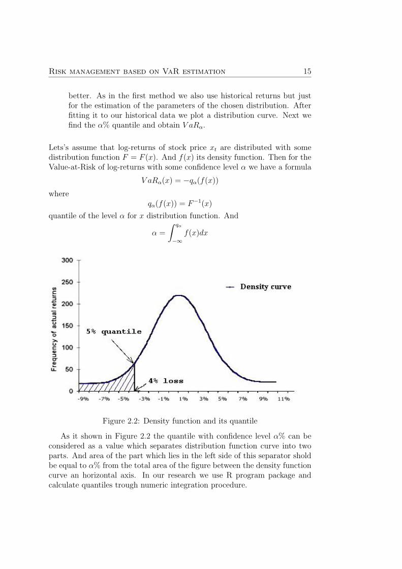
better. As in the first method we also use historical returns but justfor the estimation of the parameters of the chosen distribution. Afterfitting it to our historical data we plot a distribution curve. Next wefind the α% quantile and obtain V aRα.

Lets’s assume that log-returns of stock price xt are distributed with somedistribution function F = F (x). And f(x) its density function. Then for theValue-at-Risk of log-returns with some confidence level α we have a formula

V aRα(x) = −qα(f(x))

whereqα(f(x)) = F−1(x)

quantile of the level α for x distribution function. And

α =

∫ qα

−∞f(x)dx

Figure 2.2: Density function and its quantile

As it shown in Figure 2.2 the quantile with confidence level α% can beconsidered as a value which separates distribution function curve into twoparts. And area of the part which lies in the left side of this separator sholdbe equal to α% from the total area of the figure between the density functioncurve an horizontal axis. In our research we use R program package andcalculate quantiles trough numeric integration procedure.


Chapter 3

Methods

3.1 Volatility estimation

For our risk management purposes we will use some models as a volatilityestimator. They were introduced in the chapter above. And here we takea closer look to the models, show how to estimate parameters and makeone-step forecast using them.

• Non− parametricNonparametric regression is a fast growing direction in statistical analy-sis. There are many theoretical developments made in this field. A veryinteresting thing about the nonparametric models is that it is possibleto use them to uncover the volatility of a process that is masked bysome noise.The information that we do know is the historical log-returns ∆Xt thatconsist of the signal σt and a noise ∆Lt:

∆Xt = σt∆Lt

To make further estimations easier let’s put the equation to the powerof two and pass to the logarithm:

log (∆Xt)2 = log σ2

t + log(∆Lt)2

Our goal is to estimate the hidden volatility from the observations. Thestrength of fluctuations of log-returns mainly depends on the volatilityand the noise gives just some extra perturbation. So in such situation itis convenient to use a non-parametric smoothing (cf. Hardle (1991))[19]which will consider the noise as some error. In our research we use a

17

18 Chapter 3. Methods

moving average method:

log σt2 =

1

k

k−1∑i=0

log (∆Xt−i)2

Where k is a correctly chosen smoothing parameter. There are severalpossibilities to choose the k. It is possible to set it ”by eye” by tryingseveral values and choosing the best result. But such method is toosubjective and depends on a researcher very much. In our work we usecross-validation method which idea is in minimizing the function:

CV (k) =1

T

T∑t=1

(log (∆Xt)2 − (log σt

2)−t)2

Here T is a total number of available data points (in our case it is 499)and:

(log σt2)−t =

1

k

k∑i=1

log (∆Xt−i)2

is the same moving average but with the window moved one observa-tion back as if the information at time t is missing. So according tothis method the optimal window is such ”k” that minimizes the CVfunction and CV is actually a sum of errors.We applied this method to our 499 data set taken from the DAX andOMX indexes. In the paper of Eberlein, Kallsen and Kristen (2003)[10]authors were using the same data set and tried windows varying from5 to 80 with step 5. As a result they obtained the optimal window thatturned out to be 40. We created an application using the R packagethat calculates the CV function for the same set of windows from 5 to80 but with step 1. As a result we obtained a more precise result. It isnecessary to mention that in fact to be able to examine this set of win-dows we had to extend the data set from 499 to 579. It was necessaryto do so because the moving average method needs 80 observations be-fore the point that we want to start with to use the maximum window.The code of the application is presented in the appendix. But lets getback to our results. For the date set taken from the DAX index theoptimal window is 35 with CV equal to 9.68452. While the window 40showed CV equal to 9.705831. After applying this method to the dateset taken from the OMX index the optimal window turned out to be36 with CV equal to 7.409330 and the window 40 performed CV equalto 7.445528. To say in advance while calculating VaR we used both 35


and 40 for DAX and 36 and 40 for OMX to be able to compare theresults and to find out whether such slight difference in windows willaffect the final amount of overlaps. But first we used these windowsto estimate the volatility and obtained next graphs in Figure 4.3 andFigure4.4.We should not forget that σ2

t is affected by the expectation of (log ∆Lt)2

and for different Levy processes it is different. But since the Levyprocess can be multiplied by any constant we do not have to compen-sate for this affection.Finally we have estimated the volatility of our log-returns, but we havenot introduced any model for σ. So how are we going to create aone-period prediction for σt+1. In chapter 1 we have assume that theendurance of volatility changes is longer than the interval of the his-torical observations. So it is logical to say that tomorrow volatility ismore likely to be the same as a day before σt.

• GARCH(1,1)−MRemind the basic formula for the model

σ2t = a0 + a1σ

2t−1(∆L

2t−1 −m)2 + b1σ

2t−1 (3.1)

Thus we have to find just four unknown parametersω, α, β, m. Usu-ally estimation procedure is performed by using Maximum Likelihoodmethod. Let’s assume that ∆Lt are distributed with some distribution,which has density function f(·, θ), where θ is a set of parameters of thisdistribution.Suppose we have an initial vector of log-returns x1, .., xT Then thelikelihood function for the given data will have a form

LhoodT =T∏t=1

lt =T∑t=1

lt

where

lt = log lt = lt(xt, (xs)s=1,...,t−1, ω, α, β, m, θ) = log f(∆xtσt

, θ)

We should maximize function Lhoodt by the vector of model parametersω, α, β, m and such optimal vector gives an estimator for desirableparameters. In our research we use the R program which perform opti-mization and parameter estimation using SQP algorithm. It is based onthe normal distribution, i.e. supposes ∆Lt to be normally distributed.If we consider non-normal increments, then as it was shown Gourieroux


(1984)[17] in this case nevertheless Quasi-Maximum likelihood estima-tor (QMLE) appears to be consistent.For our Value-at-Risk calculation procedure we need one step of predic-tion for the volatility time series. Value σT+1 can be obtained directlyfrom the equations 2.1 and 3.1.

• UHF−GARCH(1,1)In order to estimate parameters of this model and receive one stepforecast for the volatility we should find estimator of duration predictedvalue first. It means we have to investigate ACD model. Remind themain formula for EACD(1,1)

p(∆t|ψt) =1

ψte−∆tψt

whereψt = ω + α∆t−1 + βψt−1 (3.2)

We apply the MLE method and use similar procedure as for the GARCH(1,1)model. EACD(1,1) log-likelihood function for the given vector of du-rations ∆1, .., ∆T looks like that

LhoodT =T∑t=1

[logψt +

∆t

ψt

]The estimation procedure will be similar in the case of Weibull ACD

g(∆k) =γ

∆k

(∆k

φk

)γ

e−

∆kφk

γ∀∆k > 0

whereφk = ω + α∆k−1 + βφk−1 (3.3)

φk =ψk

Γ(1− 1

γ

)Then log-likelihood function for WACD

LhoodT =T∑t=1

[log

γt∆t

+ γ log∆t

φt−

(∆t

φt

)γ]Maximizing Lhoodt we can receive vector of parameters ω, α, β. Hereour risk management purposes limits us with the estimation time. Be-cause it will be useless at all if the program search for an estimator


of duration longer than this duration period of time itself. We needquicker algorithms, that is why we use another parameter estimationmethod in R, call Nlminb, which is fast enough.Conditional mean of ∆t is ψt. Hence we take ψt as a predictor the nextduration. This value can be obtained through the formulas 3.2 and 3.3for EACD and WACD correspondingly. Now we are ready to estimateparameters of the UHF-GARCH(1,1).

σ2t = a+ bε2t−1 + cσ2

t−1 + d∆−1t (3.4)

where ε is as in 2.2. Log-likelihood function in this case looks like that

LhoodT = −1

2

T∑t=1

[log 2πσ2

t +ε2tσ2t

]We apply QMLE method and as before receive vector of desirable pa-rameters a, b, c, d. One step forecast for the volatility σT+1 can beobtained directly from the equation 3.4

3.2 The driving Generalized Hyperbolic process

estimation

In order to obtain consistent prediction Value-at-Risk we should know dis-tribution of the increment ∆Lt from the equation 2.1. Further we will seehow it can be applied for the VaR calculation.Advantages of Generalized Hyperbolic class of distributions and reasons totake it as a distribution of the driving process were described in the previouschapter. With such assumption for the process ∆Lt we have to estimate fiveparameters a, b, µ, β, ν of the density function fGH from the equation 2.4.Standard procedure to do it is Maximum Likelihood estimation method.Thus for the given vector of log-returns x1, .., xT we obtain log-likelihoodfunction of the following form

LhoodT =T∑t=1

fGH(x; a, b, µ, β, γ)

Common MLE procedure supposes search for the optimal set of parametersthrough the maximization of log-likelihood function over desirable parame-ters. However it is rather complicated to use this one for our purposes becausewe have to access values of five parameters and perform maximization pro-cedure also over covariance matrices.


In the R program this estimation of parameters is performed by using theiteration MCECM scheme and BFGS optimization algorithm. For furtherdetails about these procedures see Breymann, Luthi (2008)[5].In our risk management approach we assume that the next day log-returnhas the same distribution, which was estimated using previous T days data.Since estimated values of parameters vary essentially depending on T, wetake the same value as in Eberlein, Kallsen and Kristen(2003)[10] T=500.

3.3 Value-at-Risk calculation

The last step in our risk management method is to calculate VaR. We want toquantify risk concerned with changes of log-returns ∆Xt. Since Value-at-Riskcan be found from the expression

V aRα(∆XT+1) = −qα(∆XT+1) (3.5)

we need to know tomorrow distribution of log-returns. In order to obtainit, following the general model 2.1 it is enough to define the distribution ofσT+1∆LT+1. Therefore we use a well-known property of Generalized Hyper-bolic distributions class, that it is closed under linear transformation.If ξ ∼ GH(a, b, µ, β, ν) then ∀A,B ∈ R, A 6= 0

Aξ +B ∼ GH(a, b, Aµ+B,Aβ, ν)

Assume ∆LT+1 has GHT+1(a, b, µ, β, ν) distribution, and σT+1 is the one-step forecast of volatility then due to above mentioned fact distribution of∆XT+1 will be GHT+1(a, b, σT+1µ, σT+1β, ν) Now we are ready to calculateα-quantile as it was shown in the section Risk management.

Chapter 4

Backtestings and conclusions

In the practical part of this paper we are going to apply the discussed modelsto the historical data which was taken from two financial indexes, the DAXIndex and the OMX Stockholm Index (OMXS30).The DAX Index is a Blue Chip stock market index which is the most usedindicator for measuring the returns of stocks that are traded on the Frank-furt Stock Exchange. It was started in 1984 and consist of the 30 largestand most traded stocks on the exchange. The DAX belongs to performance-based indexes, which means that dividends and other add-ins are includedinto the index’s final calculation. The DAX index is calculated using pricesfrom the ”Xetra” electronic trading system from 9:00 AM to 5:30 PM CentralEuropean Time. Daily trading volume of the DAX market is approximately200000 contracts, and daily price range is approximately 160 ticks. The DAXIndex includes stocks of such big and famous companies as Adidas, Bayer,BMW, Commerzbank, DaimlerChrysler, Deutsche Bank, Deutsche Boerse,Lufthansa, MAN, METRO, Siemens, Volkswagen etc.The OMX Stockholm 30 (OMXS30) is the most known and widely used in-dex in the Nordic region. It is a capitalization-weighted index and consistsof the 30 most liquid stocks that are traded on Stockholm Stock Exchangewhich is relatively small comparing to the Frankfurt Stock Exchange. TheOMXS30 displays the general movements in the stock market. The shareof each stock of the index is specified by the market capitalization of eachcompany. The OMXS30 index is calculated accordingly to the situation onSeptember 30, 1986, when the index was developed with a base level of 125.This Index is represented by stocks of such world known companies as VolvoGroup, TeliaSonera, Svenska Handelsbanken, SEB, SCANIA, Nordea, Eric-sson, Nokia, Hennes & Mauritz etc.

Using data from these two indexes we are going to test the introduced

23

24 Chapter 4. Backtestings and conclusions

volatility models and calculate the VaR. In order to do it and compare theresults we take DAX and OMX indexes daily closing data for the same pe-riod of time as in [10] which is 2nd January 1992 - 29 June 1999. Totally- 1875 observations. First 500 observations we use for the estimation rou-tine of Volatility and Hyperbolic processes. The remaining 1375 are used forbacktesting. Thus we will be able to access preciseness of the methods.Also it is interesting to mention such detail that we were able to find depen-dence in price changes between these two financial markets. This effect easyto see in the following graphics of losses. Note that near to 1200 observationin the DAX index very large losses occurred and little bit later the samesituation happened in the Nordic market.

Figure 4.1: Losses of DAX(top) and OMX(bottom) indexes during observedperiod


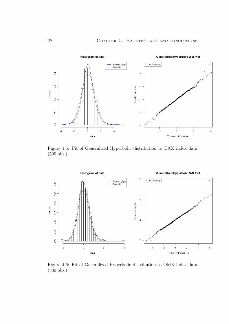
Next the estimated volatility time series for backtesting period is pre-sented on the Figure 4.2, Figure 4.3 and Figure 4.4. After that we showGeneralized Hyperbolic fit statistics for the first 500 observations data onthe Figure 4.5 and Figure 4.6. Finally on the Figures 4.7 and 4.8 Value-at-Risk illustrations are considered.We preferred not to show graphics of all the fit and Value-at-Risk for allcases of distributions. We illustrated only the best result of calculated VaRfor OMX and DAX data. All the rest of the results are presented in tablesand a corresponding analysis is given.

Figure 4.2: Volatility estimated using GARCH model for the DAX(top) andOMX(bottom) indexes


Figure 4.3: DAX Volatility estimated using Nonparametric approach withthe windows: 35(top),40 (bottom)


Figure 4.4: OMX Volatility estimated using Nonparametric approach withthe windows: 36(top),40(bottom)


Figure 4.5: Fit of Generalized Hyperbolic distribution to DAX index data(500 obs.)

Figure 4.6: Fit of Generalized Hyperbolic distribution to OMX index data(500 obs.)


Figure 4.7: V aR99% and V aR95% calculated for DAX index usingGARCH(top) and Nonparametric(bottom) models (Normal Inverse Gaussiancase)


Figure 4.8: V aR99% and V aR95% calculated for OMX index usingGARCH(top) and Nonparametric(bottom) models (Normal Inverse Gaussiancase)


Figure 4.9: Comparison of the windows used in Non-parametric model

Before discussing the preciseness of VaR calculation depending on thetype of the distribution we would like to go back to the windows that wereused in the Non-parametric model. As we mentioned before in the ”Volatilityestimation” section the optimal windows according to our research for DAXand OMX are 35 and 36 correspondingly. As provided by the Cross Vali-dation method the window 40 that was obtained in the paper of Eberlein,Kallsen and Kristen (2003)[10] showed a bit worse result. To check it practi-cally we calculated VaR for DAX and OMX using volatility calculated bothwith windows 35, 36 and 40. The results are performed in the Table 4.9.According to this table windows 35 and 36 showed better result in 9 casesand window 40 in 7 cases. So we can say that a slight change in the length ofthe window in Non-parametric model while calculating the volatility affectsthe preciseness of VaR calculation.

In our research we have found that VaR preciseness very substantiallydepends on the distribution which is used for ∆Lt. An example which isshown below illustrates the difference in DAX V aR99% estimation for theGeneralized Hyperbolic and Gaussian cases. As a result for the same back-testing period investigated models showed following behavior:


• GARCH volatility model and L∼ Generalized Hyperbolic distributed -16 overlaps

• GARCH volatility model and L∼Normally distributed - 22 overlaps

• Non parametric volatility model and L∼Generalized Hyperbolic dis-tributed - 17 overlaps

• Non parametric volatility model and L∼Normally distributed - 25 over-laps

Here ”overlap” means underestimation of returns. This example demon-strates us the fact that the accuracy of the VaR estimation depends on thetype of chosen distribution. It is obvious in the case of Normal Gaussiandistribution because even the example shows that density function differsdramatically. But in fact such differences we can observe inside the Gener-alized Hyperbolic distributions class.

Figure 4.10: Frequency of Losses Table


Figure 4.11: Losses/observation ratio

Finally due to our research and results presented on the tables above wecan conclude that the Normal Inverse Gaussian distribution satisfies our riskmanagement proposes and shows the highest level of accuracy while calcu-lating VaR.In order to check performance of the model introduced for tick data we ap-ply it to the one day Dow Jones index data. More precisely we considermovements of the index’s price during the 1st September 2004, total 10135tick observations. From the previous tests of the general model on DAXand OMXS30 indexes we have found that Normal Inverse Gaussian (NIG)distribution gives the best results. That is why we use it again as an as-sumed distribution of returns for the tick data. The fit of the distribution toempirical data looks as follows.


Figure 4.12: Fit of Normal Inverse Gaussian distribution to Dow Jones indextick data

The Figure 4.12 confirms the assumption that the quality of model’s fitis still sufficiently high in the case of tick returns. Next the 99% and 95%VaR curves obtained for Dow Jones index are presented


Figure 4.13: V aR95%(upper picture) and V aR99%(bottom picture) curvescalculated for Dow Jones index tick data using UHF-GARCH model

The Figure 4.13 reflects calculation result of Value-at-Risk for 500 tickpoints which corresponds to approximately 30 minutes of trading. In thecase of 95% VaR there were 40 overlaps and in the case of 99% VaR, 12


overlaps occured. We can see that presented method is rather robust andgives consistent results. A higher level of preciseness can be reached by usingmore complex types of ACD model. The developed method could be usefulfor those investors, who wants to make profit on very short movements ofthe price.In conclusion of our research we would like to enumerate those results thatwe obtained:

• OMX and DAX indexes are highly correlated. Furthermore losses ofNordic market repeat the tendency of losses of German market witha small lag. This effect can be easily seen when one compares twopictures on the Figure 4.1. If very high losses occur in DAX then aftersome small period of time such losses occur in OMX (pictures reflectlosses of both indexes for the same period of time).

• Estimated volatility which was obtained both using GARCH and Non-parametric models describes the shape of losses very well. It can beobserved on the Figures 4.1, 4.2, 4.3 and 4.4. This property of calcu-lated volatility is especially important for getting precise Value-at-Riskestimation.

• In Non-parametric model the windows 35 and 36 were used for DAXand OMX indexes correspondingly. They were obtained by the CrossValidation method and during backtesting performed more precise com-paring to the window 40. Respective information is shown in the Figure4.9.

• During backtesting Normal distribution performed worse than othersand Normal Inverse Gaussian showed the best outcome. It was oneof our main goals to compare Value-at-Risk calculation depending onthe distribution that is used. It is evident that Normal distributioncan not describe returns of an index as precise as Generalized Hyper-bolic distributions does. But it was interesting to obtain as a resultthat Normal Inverse Gaussian distribution due to its special propertiesperforms better than others.

• Value-at-Risk sensitivity to the choice of distribution becomes higheras the level of confidence increases.

• We have developed a model which allows us to calculate Value-at-Riskfor an intraday data. Also we have applied this model to Dow Jonesindex and have received consistent results. Actually it is possible to

model tick data using different cases of ACD and UHF-GARCH mod-els. For example using Weibull ACD model or UHF-GARCH modelwith long run volatility variable included. These improvements of thesuggested model can be considered as a subject for further research.

37

38

Appendix

Program code in RValue-at-Risk for DAX using GARCH-M model

## Take 500 work data points

z <- read.table("H:\dax.csv",sep=",", skip=1511)

y <- z[ ,5]

b=c(length(y),NA)

for (i in 1:length(y))

b[i]=y[length(y)-i+1]

x<-diff(log(b))

print(x)

## Backtesting 459 data points

2009

z1<- read.table("H:\dax.csv",sep=",", skip=133)

y1<- z1[ ,5]

b1=c(length(y1),NA)

for (i in 1:length(y1))

b1[i]=y1[length(y1)-i+1]

print(b1)

x1<-diff(log(b1))

print(x1)

plot(x1, type="p")

## Excessive loses sequence for the Backtesting data

loses=c(1378, NA)

for (i in 500:1877)

if (x1[i]<0)

loses[i-499]=-x1[i]

else loses[i-499]=0

plot(loses, type="h")

##Prices loses

z2<- read.table("H:\dax.csv",sep=",", skip=133)

y2<- z2[ ,5]

b2=c(length(y2),NA)



print(b2)

x3<-diff(b2)

print(x3)

plot(x3, type="h")


Pdloses=c(1378, NA)

39

for (i in 500:1874)

if (x3[i]<0)

Pdloses[i-499]=-x3[i]

else Pdloses[i-499]=0

plot(Pdloses, type="h")

lines(loses, type="h", col="blue")

##------------------------------

## Volatility GARCH sequence

fit = garchFit(~garch(1, 1), x)

print(fit)

Interactive Plot:

plot(fit1, which=2)

plots,results

Batch Plot:

plot(fit, which = 2)

summary(fit)

##devolatilized returns

L=x/[email protected]

print(L)

##Normal Inverse Gaussian fit

NIGfit<-fit.NIGuv(L)

hist(NIGfit, ghyp.col="blue")

qqghyp(NIGfit, gaussian=FALSE)

##---------------------

## Quantity of overlaps

Calc=function(varf)

num<-c(2008,NA)

k=0

d=0

for (i in 500:1877)

if (varf[i]<=loses[i-499])

k=d+1

d=k

num[k]=i

print(k)

print(num)

Calc=k

##-----------------

## myGarch 1 step

mygarch=function(sigma1,L1,m,c,a,b)

mygarch=sqrt(c+a*sigma1*sigma1*(L1-m)*(L1-m)+ b*sigma1*sigma1)

##----------------

## VaR 1:499

var<-c(2008,NA)

for (i in 1:499)

fitgh<-transform(‘NIGfit‘,0,[email protected][i])

lambda=qghyp(0.01,fitgh)

40

var[i]=-lambda;

##-----------

##(NIGfit) Value-at-Risk

for (i in 499:2008)

j=i-498

window<-x1[j:i]

g=garchFit(~garch(1, 1), window)

L=window/[email protected]


sd=mygarch([email protected][499],L[499],g@fit$coef[1],

g@fit$coef[2],g@fit$coef[3],g@fit$coef[4])

fitgh<-transform(‘NIGfit‘,0,sd)


var[i+1]=-lambda;

print(Calc(var))


lines(var, type="l",col="red")

##--------------------------

##Take Image out in the file

jpeg(filename="H:\QQplot for NIG.jpg")

qqghyp(NIGfit,gaussian=FALSE)

dev.off()

##-----------

41

Value-at-Risk for OMX using GARCH-M model

## Take 500 work data points

z <- read.table("H:\omx1.txt", sep="", skip=4)

y <- z[ ,5]

b=c(length(y),NA)



x<-diff(log(b))

print(x)

## Backtesting 459 data points

z <- read.table("H:\omx1.txt", sep= "", skip=4, nrows=500)

y <- z[ ,2]

x<-diff(log(y))

print(x)

z1 <- read.table("H:\omx1.txt", sep= "", skip=4)

y1 <- z1[ ,2]

x1<-diff(log(y1))

x2<-diff(y1)


loses=c(1378, NA)

for (i in 500:1877)

if (x1[i]<0)

loses[i-499]=-x1[i]

else loses[i-499]=0


## Excessive PRICE loses sequence for the Backtesting data

Ploses=c(1378, NA)

for (i in 500:1877)

if (x2[i]<0)

Ploses[i-499]=-x2[i]

else Ploses[i-499]=0

plot(Ploses, type="h")

##------------------------------

## Volatility GARCH sequence

fitOmx = garchFit(~garch(1, 1), x)

Interactive Plot:

plot(fitOmx, which=2)

##devolatilized returns

OmxL=x/[email protected]

print(OmxL)

##GH fit

fitted<-fit.ghypuv(OmxL, silent=TRUE)

hist(Omxfit, ghyp.col="blue")

qqghyp(Omxfit, gaussian=FALSE)

##---------------------


Calc=function(varf)

num<-c(2008,NA)

k=0

d=0

for (i in 500:1877)

42

if (varf[i]<=loses[i-499])

k=d+1

d=k

num[k]=i

print(k)

print(num)

Calc=k

##-----------------

## myGarch 1 step

mygarch=function(sigma1,L1,m,c,a,b)

mygarch=sqrt(c+a*sigma1*sigma1*(L1-m)*(L1-m)+ b*sigma1*sigma1)

##----------------

## VaR 1:499

var<-c(1878,NA)

for (i in 1:499)

fitgh<-transform(‘fitted‘,0,[email protected][i])


var[i]=-lambda;

##-----------

##(GH) Value-at-Risk

var<-c(1878,NA)

Curve<-c(1378,NA)

for (i in 499:1877)

j=i-498

window<-x1[j:i]

g=garchFit(~garch(1, 1), window)

L=window/[email protected]

Ggfit<-fit.ghypuv(L)

sd=mygarch([email protected][499],L[499],g@fit$coef[1],

g@fit$coef[2],g@fit$coef[3],g@fit$coef[4])

Curve[j]=sd

fitgh<-transform(‘Ggfit‘,0,sd)


var[i+1]=-lambda;

plot(Curve)

Calc(var)

Rvar<-var[500:1877]

Losses<-c(1879,NA)

Losses<-loses[1:1378]

Losses[1379]=0.15

plot(Losses, type="h", col="white")

lines(loses,type="h")

##--------------------------

##Take Image out in the file

jpeg(filename="H:\QQplot for GH.jpg")

qqghyp(fitted,gaussian=FALSE)

dev.off()

##-----------

43

Value-at-Risk for Dow Jones tick data

library(fGarch)

library(ghyp)

##Data

hh<-read.table("D:\dj_tick.csv",sep=",", skip=1, nrows=10000)

pr<-hh[,4]

plot(pr,type="l")

ff<-(log(pr))

plot(ff,type="l")

r<-diff(ff)

plot(r,type="l")

Losses<-c(500)

for(i in 500:9999)

if (r[i]<0)

Losses[i-499]=-r[i]

else

Losses[i-499]=0

tm<-hh[,3]

ttt<-timeDate(paste(tm), format = "%H:%M:%S")

dt<-diff(ttt)

d<-as.numeric(dt)

rLosses<-c(500)

eps=r/sqrt(d)

for(i in 500:9999)

if (r[i]<0)

rLosses[i-499]=-r[i]

else

rLosses[i-499]=0

plot(rLosses[1:9499],type="h")

##---------------------------------

## ACD parameters estimation

dur<-d[1:499]

lhood<-function(teta,dur)

psi<-c(499,NA)

if (teta[1]/(1-teta[3])>0)

psi[1]=teta[1]/(1-teta[3])

for(i in 2:499)

psi[i]=teta[1]+teta[2]*dur[i-1]+teta[3]*psi[i-1]

lhood=sum(log(psi)+dur/psi)

else

lhood=Inf

predict<-function(dur,a,b,c)

psi<-c(500,NA)

psi[1]=a/(1-c)

for(i in 2:500)

44

psi[i]=a+b*dur[i-1]+c*psi[i-1]

predict=psi[500]

##---------------------------------

## UHF-GARCH parameters estimation

ret<-r[1:499]

eps<-ret/sqrt(dur)

Vlhood<-function(theta,eps,dur)

sig<-c(499,NA)

if( theta[1]*(1-theta[2]-theta[3])> 0)

sig[1]=sqrt(theta[1]/(1-theta[2]-theta[3]))

for(i in 2:499)

if ((theta[1]+theta[2]*eps[i-1]^2+theta[3]*sig[i-1]^2+theta[4]/dur[i])>0)

sig[i]=sqrt(theta[1]+theta[2]*eps[i-1]^2+theta[3]*sig[i-1]^2+theta[4]/dur[i])

else sig[i]=Inf

Vlhood=sum(log(2*pi*sig^2)+(eps/sig)^2)/2

else

Vlhood=Inf

predictVol<-function(vect,eps,d1)

sig<-c(500,NA)

sig[1]=sqrt(vect[1]/(1-vect[2]-vect[3]))

for(i in 2:500)

sig[i]=sqrt(vect[1]+vect[2]*eps[i-1]^2+vect[3]*sig[i-1]^2+vect[4]/d1[i])

predictVol=sig[500]

Vol<-function(vect,eps,d1)

sig<-c(500,NA)

sig[1]=sqrt(vect[1]/(1-vect[2]-vect[3]))

for(i in 2:500)

sig[i]=sqrt(vect[1]+vect[2]*eps[i-1]^2+vect[3]*sig[i-1]^2+vect[4]/d1[i])

Vol=sig

##----Shape of the distribution----------

shape<-function(f)

x<-c(200000,NA)

y<-c(200000,NA)

x[1]=-0.0003

y[1]=dghyp(0.0001,fitgh)

for (i in 2:40)

k=-0.0001+i*0.00001

x[i]=k

y[i]=dghyp(k,fitgh)

plot(x,y,type="l")

45

shape(fitgh)

##My Quantile-------------------------

f<-function(x)

f<-dghyp(x,fitgh)

quant1<-function(q)

k=0

p=1

a=-0.1

b=0

x=(a+b)/2

ind=0

while((abs(q-p)>1e-6)&&(k<=1000))

if (ind==0)

k1=k

k=k1+1

x=(a+b)/2

if(integrate(f, -0.1, x, stop.on.error = FALSE)$message=="OK")

ind=0

I<-integrate(f, -0.1, x, stop.on.error = FALSE)

p=I$value

if (q<p)

b=x

side=-1

else

a=x

side=1

else

x1=x

if (side==1) x=x1+0.0001

else x=x1-0.0001

ind=1

print(k)

print(p)

quant1<-x

q<-quant1(0.01)

q

##-----------------------------------

square<-function(f)

I<-integrate(f, -0.1, 0.1)

square<-I$value

print(square(fitgh))

##------------------------


Calc=function(var, n1, n2)

46

num<-c(501,NA)

k=0

d=0

for (i in n1:n2)

if (var[i]<rLosses[i])

k=d+1

d=k

num[k]=i

print(k)

print(num)

Calc=k

##--------------------------------------------

##------VaR-----

tvar<-c(10000,NA)

for (i in 499:9999)

j=i-498

w<-d[j:i]

r499<-r[j:i]

eps499<-r499/sqrt(w)

sg0=sum(eps499^2)/499

teta0<-c(sg0,1/4,1/4)

##teta0<-c(1/2,1/4,1/4)

opt<-nlminb(start = teta0, lhood, d = w)

vect1<-c(opt$par[1],opt$par[2],opt$par[3])

d500<-w

d500[500]=predict(w,vect1[1],vect1[2],vect1[3])

theta0<-c(sg0,3/16,3/16,2/16)

##theta0<-c(1/2,1/6,1/6,1/6)

opt1<-nlminb(start = theta0, Vlhood, eps=eps499, d = w, lower=1e-10, upper=5)

vect2<-c(opt1$par[1],opt1$par[2],opt1$par[3],opt1$par[4])

sig=Vol(vect2,eps499,d500)

sigma=sig*sqrt(d500)

L=eps499/sigma[1:499]

NIGfit<-fit.ghypuv(L)

fitgh<-transform(‘NIGfit‘,0,sigma[500])

shape(fitgh)

lambda<-quant1(0.01)

tvar[j]=-lambda;

tvar[1:9501]

plot(rLosses[1:9501],type="h")

lines(tvar[1:9501], type="l", col="blue")

Calc(tvar,1,9500)

##----------------

47

Finding the optimal window for Non-parametric modelusing CV method

## Working with data from DAX ------------------------------------------------------

## Loading 500 data points from the file--------------------------------------------

z <- read.table("D:\dax.csv",sep=",", skip=1431)

y <- z[ ,5]

b=c(length(y),NA)



## Calculating log-returns ----------------------------------------------------------

x<-diff(log(b))

print(x)

## After calculating log-returns in some points we obtain zeros that we can not

use, so we replace them with a very small value 1e-10 -------------------------------

zeros<-c(579,NA)

id=1

for(i in 1:579)

if (x[i]==0)

x[i]=1e-10

zeros[id]=i

id=id+1

zeros

## This function is ((log(b^2)^-t) and is used to calculate CV function ------------

sigma=function(k,x,l)

d=0

vec<-x[1:l]

vec1<-log(vec^2)

for(i in 1:k)

a=l-i

d=d+vec1[a]

sigma=d/k

mas<-log(x^2)

## This is CV function -------------------------------------------------------------

CV=function(k,mas,x,T)

s=0

for(j in 1:T)

l=j+80

s=s+(mas[l]-sigma(k,x,l))^2

CV=s/T

48

## This shows all the values of CV function calculated for different "k" and then finds

the optimal window by choosing the smallest one ------------------------------------

T=499

ff<-c(200,NA)

min=CV(5,mas,x,T)

window=5

min

k=5

while(k<=80)

ff[k]=CV(k,mas,x,T)

if (ff[k]<min)

min=ff[k]

window=k

k=k+1

ff

window

## Working with data from OMX ------------------------------------------------------

## Algorithm and the body of the program are the same, we change only the part that

loads data points from the file ----------------------------------------------------

z <- read.table("D:\omx1.txt",sep="", skip=4, nrows=580)

y <- z[ ,2]

print(y)

x<-diff(log(y))

print(x)

49

Value-at-Risk for DAX using Non-parametric model

## Loading data points from the file------------------------------------------------

z1<- read.table("D:\dax.csv",sep=",", skip=2)

y1<- z1[ ,5]

b1=c(length(y1),NA)



print(b1)


x1<-diff(log(b1))

print(x1)

plot(x1, type="h")

## Finding excessive loses sequence for Backtesting and obtaining it’s graphic -----

loses=c(length(x1), NA)

for (i in 1:length(x1))

if (x1[i]<0)

loses[i]=-x1[i]

else loses[i]=0


lines(loses, type="h", col="blue")

## A function that predicts volatility one step forward ----------------------------

sigma=function(k,x,t)

d=0

vec<-x[1:t]

vec1<-log(vec^2)

for(i in 1:k)

if(is.finite(vec1[t-i]))

d=d+vec1[t-i]

sigma=d/k

## A function that calculates volatility for distribution’s parameters estimation --

sigmad=function(k,x,t)

d=0

vec<-x[1:t]

vec1<-log(vec^2)

for(i in 0:k-1)


d=d+vec1[t-i]

sigma=d/k

## Calculating volatility using window 35 to find VaR ------------------------------

volatility35<-c(1973,NA)

k=35

for (i in 36:2008)

volatility35[i-35]=sqrt(exp(sigma(k,x1,i)))

volatility35

## Calculating volatility using window 35 to estimate distribution’s parameters ----

volatilityd35<-c(1973,NA)

k=35

50

for (i in 35:2008)

volatilityd35[i-34]=sqrt(exp(sigmad(k,x1,i)))

volatilityd35

## Calculating VaR 1% using GENERALIZED HYPERBOLIC DISTRIBUTION --------------------

var35GHYP<-c(2008,NA)

for (i in 533:2008)

j=i-498

a=j-34

b=i-34

c=i-33

window<-x1[j:i]

v1<-volatilityd35[a:b]

L=window/v1

GHYPfit<-fit.ghypuv(L)

fitgh<-transform(‘GHYPfit‘,0,volatility35[c])


var35GHYP[i+1]=mean(fitgh)-lambda;

## Calculating the number of overlaps and finding points where they occurred -------

Calc=function(varf)

num<-c(2008,NA)

k=0

d=0

for (i in 1:1474)

if (varf[i]<=Loses[i])

k=d+1

d=k

num[k]=i

print(k)

print(num)

Calc=k

## Drawing graphics of losses and VaR 1% -------------------------------------------

var35GHYPplot<-c(1475,NA)

var35GHYPplot<-var35GHYP[534:2007]

Losses<-c(1475,NA)


Losses[1475]=0.18

Loses<-loses[534:2007]


lines(Loses, type="h")

lines(var35GHYPplot, type="l",col="red")

Calc(var35GHYPplot)

var35GHYPplot

## To calculate VaR 5% using GENERALIZED HYPERBOLIC DISTRIBUTION we follow the same

steps that were shown above for calculating VaR 1% but the line

"lambda=qghyp(0.01,fitgh)" should be changed to "lambda=qghyp(0.05,fitgh)"

## To calculate VaR using other distributions we take the same procedure as shown

above but with following changes ------------------------------------------------

## VaR 1% using HYPERBOLIC DISTRIBUTION --------------------------------------------

...

51

var35HYP<-c(2008,NA)

for (i in 533:2008)

j=i-498

a=j-34

b=i-34

c=i-33

window<-x1[j:i]


L=window/v1

HYPfit<-fit.hypuv(L)

fith<-transform(‘HYPfit‘,0,volatility35[c])

lambda=qghyp(0.01,fith)

var35HYP[i+1]=mean(fith)-lambda;

...


lambda=qghyp(0.01,fith) -----> lambda=qghyp(0.05,fith)

## VaR 1% using NORMAL INVERSE GAUSSIAN --------------------------------------------

...

var35NIG<-c(2008,NA)

for (i in 533:2008)

j=i-498

a=j-34

b=i-34

c=i-33

window<-x1[j:i]


L=window/v1


fitnig<-transform(‘NIGfit‘,0,volatility35[c])

lambda=qghyp(0.01,fitnig)

var35NIG[i+1]=mean(fitnig)-lambda;

...


lambda=qghyp(0.01,finig) -----> lambda=qghyp(0.05,fitnig)

## VaR 1% using NORMAL GAUSSIAN DISTRIBUTION ---------------------------------------

...

var35GAUSS<-c(2008,NA)

for (i in 533:2008)

j=i-498

a=j-34

b=i-34

c=i-33

window<-x1[j:i]


L=window/v1

par<-coef(GAUSSfit)

fitgauss<-gauss(par$mu, volatility35[c]*par$sigma)

lambda=qghyp(0.01,fitgauss)

var35GAUSS[i+1]=mean(fitgauss)-lambda;

...

52


lambda=qghyp(0.01,fitgauss)-----> lambda=qghyp(0.05,figauss)

## VaR 1% using Variance Gamma -----------------------------------------------------

...

var35VG<-c(2008,NA)

for (i in 533:2008)

j=i-498

a=j-34

b=i-34

c=i-33

window<-x1[j:i]


L=window/v1

VGfit<-fit.VGuv(L)

fitvg<-transform(‘VGfit‘,0,volatility35[c])

lambda=qghyp(0.01,fitvg)

var35VG[i+1]=mean(fitvg)-lambda;

...


lambda=qghyp(0.01,fitvg)-----> lambda=qghyp(0.05,fitvg)

## VaR 1% using STUDENT ------------------------------------------------------------

...

var35St<-c(2008,NA)

for (i in 533:2008)

j=i-498

a=j-34

b=i-34

c=i-33

window<-x1[j:i]


L=window/v1

Stfit<-fit.tuv(L)

fitst<-transform(‘Stfit‘,0,volatility35[c])

lambda=qghyp(0.01,fitst)

var35St[i+1]=mean(fitst)-lambda;

...


lambda=qghyp(0.01,fitst) -----> lambda=qghyp(0.05,fitst)

53

Value-at-Risk for OMX using Non-parametric

## Loading data points from the file------------------------------------------------

z1<- read.table("D:\omx1.txt",sep="", skip=4)

b1<- z1[ ,2]

print(b1)


x1<-diff(log(b1))

print(x1)

plot(x1, type="h")

## Finding excessive loses sequence for Backtesting and obtaining it’s graphic -----

loses=c(length(x1), NA)

for (i in 1:length(x1))

if (x1[i]<0)

loses[i]=-x1[i]

else loses[i]=0

plot(loses, type="l")

## A function that predicts volatility one step forward ----------------------------

sigma=function(k,x,t)

d=0

vec<-x[1:t]

vec1<-log(vec^2)

for(i in 1:k)


d=d+vec1[t-i]

sigma=d/k

## A function that calculates volatility for distribution’s parameters estimation --

sigmad=function(k,x,t)

d=0

vec<-x[1:t]

vec1<-log(vec^2)

for(i in 0:k-1)


d=d+vec1[t-i]

sigma=d/k

## Calculating volatility using window 36 to find VaR ------------------------------

volatility36<-c(1877,NA)

k=36

for (i in 37:1877)

volatility36[i-36]=sqrt(exp(sigma(k,x1,i)))

volatility36

## Calculating volatility using window 36 to estimate distribution’s parameters ----

volatilityd36<-c(1877,NA)

k=36

for (i in 36:1877)

volatilityd36[i-35]=sqrt(exp(sigmad(k,x1,i)))

volatilityd36

54

## Calculating VaR 1% using GENERALIZED HYPERBOLIC DISTRIBUTION --------------------

var36GHYP<-c(1877,NA)

for (i in 534:1877)

j=i-498

a=j-35

b=i-35

c=i-34

window<-x1[j:i]


L=window/v1

GHYPfit<-fit.ghypuv(L)

fitgh<-transform(‘GHYPfit‘,0,volatility36[c])


var36GHYP[i+1]=mean(fitgh)-lambda;

for (i in 535:1876)

if(is.na(var36GHYP[i])==TRUE)

var36GHYP[i]=var36GHYP[i-1]

## Calculating the number of overlaps and finding points where they occurred -------

Calc=function(varf)

num<-c(1342,NA)

k=0

d=0

for (i in 1:1342)

if (varf[i]<=Loses[i])

k=d+1

d=k

num[k]=i

print(k)

print(num)

Calc=k

## Drawing graphics of losses and VaR 1% -------------------------------------------

var36GHYPplot<-c(1342,NA)

var36GHYPplot<-var36GHYP[535:1876]

Losses<-c(1342,NA)


Losses[1342]=0.1

Loses<-loses[534:1876]


lines(Loses, type="h")

lines(var36GHYPplot, type="l",col="red")

Calc(var36GHYPplot)

## To calculate VaR 5% using GENERALIZED HYPERBOLIC DISTRIBUTION we follow the same

steps that were shown above for calculating VaR 1% but the line

"lambda=qghyp(0.01,fitgh)" should be changed to "lambda=qghyp(0.05,fitgh)"

## To calculate VaR using other distributions we take the same procedure as shown

above but with some changes -----------------------------------------------------

55


...

var36HYP<-c(1877,NA)

for (i in 534:1877)

j=i-498

a=j-35

b=i-35

c=i-34

window<-x1[j:i]


L=window/v1

HYPfit<-fit.hypuv(L)

fith<-transform(‘HYPfit‘,0,volatility36[c])

lambda=qghyp(0.01,fith)

var36HYP[i+1]=mean(fith)-lambda;

...


lambda=qghyp(0.01,fith) -----> lambda=qghyp(0.05,fith)


...

var36NIG<-c(1877,NA)

for (i in 534:1877)

j=i-498

a=j-35

b=i-35

c=i-34

window<-x1[j:i]


L=window/v1


fitnig<-transform(‘NIGfit‘,0,volatility36[c])

lambda=qghyp(0.01,fitnig)

var36NIG[i+1]=mean(fitnig)-lambda;

...


lambda=qghyp(0.01,fitnig)-----> lambda=qghyp(0.05,fitnig)


...

var36GAUSS<-c(1877,NA)

for (i in 534:1877)

j=i-498

a=j-35

b=i-35

c=i-34

window<-x1[j:i]


L=window/v1

GAUSSfit<-fit.gaussuv(L)

par<-coef(GAUSSfit)

fitgauss<-gauss(par$mu, volatility36[c]*par$sigma)

56

lambda=qghyp(0.01,fitgauss)

var36GAUSS[i+1]=mean(fitgauss)-lambda;

...


lambda=qghyp(0.01,fitgauss)-----> lambda=qghyp(0.05,fitgauss)


...

ar36VG<-c(1877,NA)

for (i in 534:1877)

j=i-498

a=j-35

b=i-35

c=i-34

window<-x1[j:i]


L=window/v1

VGfit<-fit.VGuv(L)

fitvg<-transform(‘VGfit‘,0,volatility36[c])

lambda=qghyp(0.01,fitvg)

var36VG[i+1]=mean(fitvg)-lambda;

...


lambda=qghyp(0.01,fitvg)-----> lambda=qghyp(0.05,fitvg)


...

var36St<-c(1877,NA)

for (i in 534:1877)

j=i-498

a=j-35

b=i-35

c=i-34

window<-x1[j:i]


L=window/v1

Stfit<-fit.tuv(L)

fitst<-transform(‘Stfit‘,0,volatility36[c])

lambda=qghyp(0.01,fitst)

var36St[i+1]=mean(fitst)-lambda;

...


lambda=qghyp(0.01,fitst)-----> lambda=qghyp(0.05,fitst)

57

58

Bibliography

[1] Barndorff-Nielsen O.(1998)Process of normal inverse Gaussian type. Finance & Stochastics 2, pp.41-68

[2] Barone-Adesi G., Giannopoulos K. and Vosper L.(1999)VaR without correlations for nonlinear portfolios. Journal of FuturesMarkets 19 (1999), pp. 583-602

[3] Black F. and Scholes M.S.(1973)The Pricing of Options and Corporate Liabilities. Journal of PoliticalEcomomy 81, pp. 637-654

[4] Bollerslev T.(1986)Generalized autoregressive conditional heteroscedasticity. Journal ofEconometrics 31, pp. 307-327

[5] Breymann W. and Luthi D.(2008)ghyp: A package on generalized hyperbolic distributions .R documentation, http://www.r-project.org/, CRAN, Packages, ghyp.

[6] Buhlmann P. and McNeil A.J.(2002)An Algorithm for Nonparametric GARCH modeling.Computational Statistics and Data Analysis, Volume 40, Number 4, pp.665-683

[7] Eberlein E. and Keller U., University of Freiburg (1995)Hyperbolic Distributions in Finance.Bernoulli Journal, Vol. 1, No. 3, pp. 281-299

[8] Eberlein E.(2001)Application of Generalized Hyperbolic Levy motions to Finance.In Barndorff-Nielsen O., Mikosch T. and Resnick S., Levy Processes:Theory and Application, pp. 319-337

59

[9] Eberlein E. and Prause K.(2002)The generalized hyperbolic model: Financial derivatives and risk mea-sures. In Geman H., Madan D., Pliska S. and Vorst T. MathematicalFinance - Bachelier Congress 2000, pp. 245-267

[10] Eberlein E., Kallsen J. and Kristen J.(2003)Risk management based on stochastic volatility. The Journal of Risk,Vol. 5, No. 2, pp. 19-44

[11] Eberlein,E. and Ozkan F.(2003)Time consistency of Levy models. Quantitative Finance, Vol. 3, pp. 40-50

[12] Eberlein,E., Keller U. and Prause K. University of Freiburg, (1998)New Insights into Smile, Mispricing, and Value at Risk: The HyperbolicModel.The Journal of Business, Vol. 71, No. 3, pp. 371-405.

[13] Engle R.F. and Russel J.R.(1998)Autoregressive Conditional Duration: A new model for irregularityspaced transaction data. Econometrica, Vol.66, No.5, pp. 1127-1162

[14] Engle R.F. (2000)The econometrics of Ultra-High-Frequency data. Econometrica, Vol.68,No.1, pp. 1-22

[15] Engle R.F. and Russel J.R.(2006)Analysis of High Frequency financial data. In Ait Sahalia, Y., Hansen,L.P. (Eds.), Handbook of Financial Econometrics.

[16] Gay D.M.(1990)Usage Summary for Selected Optimization Routines. Computation Sci-ence Technical Report No. 153, Murray Hill: AT&T Bell Laboratories.

[17] Gourieroux C., Monfort A. and Trognon A. (1984)Pseudo Maximal Likelihood Methods: Application to Poisson Models.Econometrica. May 1984, Vol. 52, No. 3, pp. 701-720.

[18] Guermat C. and Harris R. (2002)Robust Conditional Variance Estimation and Value-at-Risk. Journal ofRisk, Vol. 4, No. 2, pp. 25-41

[19] Hardle W. (1991)Applied Nonparametric Regression. Econometric Society Monograph Se-ries 19, Cambridge University Press, ISBN 0-521-42950-1, p. 333

60

[20] Hu W. (2005)Calibration of multivariate generalized hyperbolic distributions using theEM algorithm, with applications in risk management, portfolio optimiza-tion, and portfolio credit risk. PhD dissertation, Florida State University,2005 .

[21] Hull J. and White A. (1998)Incorporating volatility updating into the historical simulation methodfor Value at Risk. Journal of Risk, Vol. 1, pp. 5-19

[22] Markowitz H. (1952)Portfolio Selection. The Journal of Finance, Vol.7, No.1, pp. 77-91.

[23] McNeil A.J. and Frey R.(2000)Estimation of tail-related risk measures for heteroskedastic financial timeseries: An extreme value approach. Journal of Empirical Finance, Vol.7, pp. 271-300

[24] Shephard N.(1996)Statistical aspect of ARCH and stochastic volatility In Cox D., HinkleyD. and Brandorff-Nielsen O. Time Series Models, pp. 1-67. London:Chapman and Hall.

[25] Shiryaev A.N.(1998)Foundation of Stochastic financial mathematics. Fazis, Moscow 1998;English transl., Essentials of stochastic finance: facts, models, theory.Singapore, River Edge, NJ 1999, World Scientific, Vol. 1,2.

[26] Venter J. and de Jongh P.(2002)Risk estimation using the normal inverse Gaussian distribution. Journalof Risk 4, pp. 1-23

61

Documents

Risk management based on GARCH and Non …239419/FULLTEXT01.pdfGARCH and Non-parametric stochastic volatility models and some cases of Generalized Hyperbolic distribution ... in every