Risk Management in Financial Institutions∗

Adriano A. Rampini† S. Viswanathan‡ Guillaume Vuillemey§

This draft: April 2016First draft: October 2015

Abstract

We study risk management in financial institutions using data on hedging ofinterest rate risk by U.S. banks and bank holding companies. Theory predicts thatmore financially constrained institutions hedge less and that institutions whose networth declines due to adverse shocks reduce hedging. We find strong evidenceconsistent with the theory both in the cross-section and within institutions overtime. For identification, we exploit net worth shocks resulting from loan lossesdue to drops in house prices. Institutions which sustain such losses reduce hedgingsubstantially relative to otherwise similar institutions. We find no evidence thatrisk shifting, changes in interest rate risk exposures, or regulatory capital explainhedging behavior.

Keywords: Risk management; Financial institutions; Interest rate risk; Financialconstraints; DerivativesJ.E.L. Codes: G21, G32, D92, E44

∗We thank Manuel Adelino, Markus Brunnermeier, Divya Kirti, João Santos, David Scharfstein,Jeremy Stein, Adi Sunderam, James Vickery, and seminar participants at Duke University, HEC Paris,Princeton University, Georgia State University, the Federal Reserve Bank of New York, and the NBERInsurance and Corporate Finance Joint Meeting for helpful comments. Address: Duke University, FuquaSchool of Business, 100 Fuqua Drive, Durham, NC, 27708. Rampini: Phone: (919) 660-7797. Email:rampini@duke.edu. Viswanathan: Phone: (919) 660-7784. Email: viswanat@duke.edu. Vuillemey:Phone: +33 (0)6 60 20 42 75. Email: vuillemey@hec.fr.†Duke University, NBER, and CEPR‡Duke University and NBER§HEC Paris

1 IntroductionThe potential of the market for financial derivatives for use in risk management remainsunrealized. Limited risk management leaves financial institutions, firms, and householdsmore exposed to shocks than they could be and is arguably a key factor in financialcrises. Why the gains from using traded securities for risk management are exploitedto such a limited extent remains a central open question. To address this question, westudy the determinants of risk management in the quantitatively largest market for suchinstruments – the interest rate derivatives market – in which the main participants arefinancial institutions.

We show that the net worth of financial institutions is a principal determinant oftheir risk management: better capitalized institutions hedge more and institutions whosenet worth declines reduce hedging. We find a statistically and economically significantpositive relation between interest rate risk management and net worth both across in-stitutions and within-institution over time. Moreover, we propose a novel identificationstrategy. We instrument variation in financial institutions’ net worth using losses on realestate loans attributable to local house price shocks, and use these shocks to estimatedifference-in-differences models. We find that institutions which suffer such shocks sub-stantially reduce interest rate risk management. We also show that institutions reducehedging significantly several quarters before failing or entering financial distress. Weconclude that the financing needs associated with hedging are a major barrier to riskmanagement.

We focus on the financial intermediary sector for several reasons. First, despite muchdebate about bank risk management and its failure during the financial crisis, even thebasic patterns of risk management in financial institutions are not known and its maindeterminants are not well understood. Second, financial institutions play a key role in themacroeconomy and for the transmission of monetary policy. Understanding their exposureto interest rate shocks and the extent to which they do or do not hedge these exposures isthus essential for monetary and macro-prudential policy.1 Third, financial intermediariesare the largest users of derivatives, measured in terms of gross notional exposures, and

1Following Bernanke and Gertler (1989), the effects of the net worth of financial institutions on theavailability of intermediated finance and real activity are analyzed by Holmström and Tirole (1997),Gertler and Kiyotaki (2010), Brunnermeier and Sannikov (2014), and Rampini and Viswanathan (2015),among others. Empirically, the effects of bank net worth on lending and real activity are documented byPeek and Rosengren (1997, 2000), and its effects on employment are studied by Chodorow-Reich (2014).Financial institutions’ central role in the transmission of monetary policy is examined by Gertler andGilchrist (1994), Bernanke and Gertler (1995), Kashyap and Stein (2000), and Jiménez, Ongena, Peydró,and Saurina (2012).

1

interest rate derivatives comprise the bulk of such exposures.2 The management of interestrate risk is a primary concern of financial intermediaries; indeed, in our data on U.S.financial institutions, interest rate derivatives represent on average 94% of the notionalvalue of all derivatives used for hedging, far exceeding other derivatives positions.3

We use risk management theory to inform our measurement. A leading theory ofcorporate risk management argues that firms subject to financial constraints are effectivelyrisk averse, giving them an incentive to hedge (see Froot, Scharfstein, and Stein, 1993).Given this rationale, Rampini and Viswanathan (2010, 2013) show that in a dynamicmodel where financing and risk management are subject to the same financial constraints,that is, promises to both financiers and hedging counterparties need to be collateralized,both require net worth. Therefore, a dynamic trade-off between financing investmentor current operations and risk management arises: financially constrained firms mustallocate their limited net worth between the two. Hedging has an opportunity cost interms of foregone investment. The basic prediction of the dynamic theory is that morefinancially constrained firms, that is, firms with lower net worth, hedge less. The cost offoregoing investment or down-sizing operations is higher at the margin for such firms.

We test this prediction in panel data on U.S. banks and bank holding companies. Weshow that the theory is consistent with the main empirical patterns, which have not beendocumented previously. In the cross section, better capitalized financial intermediarieshedge interest rate risk to a greater extent. Over time, institutions whose net worthfalls reduce their hedging and institutions that approach financial distress drastically cutback on risk management. We propose a novel identification strategy by focusing ondrops in financial institutions’ net worth due to loan losses attributable to falls in houseprices. Instrumenting financial institutions’ net income with the deposit-weighted averageof changes in local house prices, we find a significant positive relation between hedgingand net worth. Using a difference-in-differences estimation and 2009 as the treatmentyear, we find that institutions (i) with a lower net income, (ii) a larger decrease in localhouse prices, and (iii) a lower local housing supply elasticity, cut hedging substantiallyrelative to institutions in the relevant control groups.4

2According to the BIS’ Derivative Statistics (December 2014), financial institutions account for morethan 97% of all gross derivatives exposures and interest rate derivatives comprise 80% of the notionalvalue of all derivatives globally.

3Other positions include foreign exchange derivatives (5.4% of notional value), equity derivatives(0.7%), and commodity derivatives (0.1%). Not included in these calculations are credit derivatives, asno breakdown between uses for hedging and trading is available.

4A growing literature uses house prices to instrument for the collateral value of firms (see, for example,Chaney, Sraer, and Thesmar, 2012) and entrepreneurs (see, for example, Adelino, Schoar, and Severino,2015). For financial institutions, a measure of local house prices in a similar spirit to ours, albeit at a

2

Importantly, we are able to rule out alternative explanations consistent with a pos-itive relation between net worth and hedging. First, we find that trading activities arealso positively related to net worth, both between and within institutions. This evidenceis not consistent with the idea that financially constrained institutions cut hedging be-cause they engage in risk shifting. Second, we show that more constrained institutions donot substitute financial hedging with operational risk management by holding more netfloating-rate assets; instead, we find that net floating-rate assets are strongly positivelyrelated to net worth and that institutions which approach distress dramatically cut theirnet floating-rate assets. If anything, institutions that do more financial hedging also domore operational hedging. Finally, we find that it is the net worth of financial insti-tutions, that is, their market value, which determines their hedging policy rather thantheir regulatory capital. Regulatory capital is not a significant determinant of bank riskmanagement.

Data availability presents a major challenge for inference regarding the determinantsof risk management. Much of the literature is forced to rely on data that includes onlydummy variables on whether firms use any derivatives or not.5 In contrast, our dataprovides measures of the intensive margin of hedging, not just of the extensive margin.Further, much of the literature has access to only cross-sectional data or data with at besta limited time dimension.6 Instead, we have panel data for U.S. bank holding companiesand banks at the quarterly frequency for up to 19 years, that is, up to 76 quarters. Thisenables us to exploit the within-variation separately from the between-variation.

The closest paper to ours in terms of the empirical approach is Rampini, Sufi, andViswanathan (2014) who study fuel price risk management by U.S. airlines. Like us, theyhave panel data on the intensive margin, albeit for a more limited sample; they havedata at the annual frequency for up to 15 years and up to 23 airlines, 270 airline-yearobservations in all, whereas we use a much larger data set. One advantage of their datais that hedging is arguably measured more precisely, as airlines report the fraction ofnext year’s expected fuel expenses that they hedge. We discuss our hedging measuresin greater detail in Section 3. One major difference is the identification strategy, aswe are able to exploit exogenous variation in net worth due to house price changes.

higher level of aggregation, is used in several recent studies of the determinants of the supply of banklending (see Bord, Ivashina, and Taliaferro (2014), Cuñat, Cvijanović, and Yuan (2014), and Kleiner(2015)).

5Guay and Kothari (2003) emphasize that such data may be misleading when interpreting the eco-nomic magnitude of risk management. Their hand-collected data on the size of derivatives hedgingpositions suggests that these are quantitatively small for most non-financial firms.

6For example, Tufano (1996)’s noted study of risk management by gold mining firms uses only threeyears of data, albeit the data is on the intensive margin of hedging.

3

Moreover, we focus on risk management in the financial intermediary sector, which is ofquantitative importance from a macroeconomic perspective and has received widespreadattention both among researchers and policy makers. Nevertheless, our basic findings areconsistent with theirs, suggesting that the specifics of the industry are not driving theresults.

When describing the basic patterns of risk management, the existing literature hasmostly emphasized a strong positive relation between firm size and hedging (see Nance,Smith, and Smithson (1993) and Géczy, Minton, and Schrand (1997) for large U.S. cor-porations). For financial institutions, the fact that users of derivatives are larger thannon-users is shown by Purnanandam (2007).7 From the vantage point of previous theories,the positive relation between firm size and hedging has long been considered a puzzle (see,for example, Stulz, 1996), because larger firms are considered less constrained. Based ona large sample of 3,022 firms, Mian (1996) reaches the stark conclusion that “evidence isinconsistent with financial distress cost models; evidence is mixed with respect to con-tracting cost, capital market imperfections and tax-based models; and evidence uniformlysupports the hypothesis that hedging activities exhibit economies of scale.”8 The hypoth-esis which we test, in contrast, is consistent with the observation that large financialinstitutions hedge more. Guided by the new dynamic theory of risk management, we arealso able to provide a much more detailed description of both cross-sectional and time-series patterns in hedging by financial institutions. We show that the key determinant ofthese patterns is not size as such, but net worth, as measured by several variables.

Finally, related to this paper is also the literature on interest rate risk in banking.Purnanandam (2007) shows that the lending policy of financial institutions which engagein derivatives hedging is less sensitive to interest rate spikes than that of non-user in-stitutions. More recently, Landier, Sraer, and Thesmar (2013) find that the exposure offinancial institutions to interest rate risk predicts the sensitivity of their lending policyto interest rates. Theoretically, the optimal management of interest rate risk by finan-cial institutions, as well as its impact on lending, is modelled by Vuillemey (2015). In arecent study, Begenau, Piazzesi, and Schneider (2015) quantify the exposure of financialinstitutions to interest rate risk. They find economically large interest rate exposuresboth in terms of balance sheet exposures and exposures due to the overall derivatives

7Ellul and Yerramilli (2013) construct a risk management index to measure the strength and inde-pendence of the risk management function at bank holding companies and find that larger institutionshave a higher risk management index, that is, stronger and more independent risk management.

8Other theories of risk management include managerial risk aversion (see Stulz, 1984) and informationasymmetries between managers and shareholders (see DeMarzo and Duffie (1995) and Breeden andViswanathan (1998)).

4

portfolios, which include trading and market making positions. In contrast, our focus ison the dynamic determinants of hedging by financial institutions based on risk manage-ment theory. The overall literature on risk management using interest rate derivatives,however, is surprisingly small, given the enormous size of this market and the centralrole of financial institutions in the macro finance nexus. Our paper contributes to abetter understanding of this market, by documenting new empirical regularities in thecross-section and time-dimension, consistent with dynamic risk management theory.

The paper proceeds as follows. Section 2 discusses the theory of risk managementsubject to financial constraints, and formulates our main hypothesis. Section 3 describesthe data and the measurement of interest rate hedging by financial institutions. Section 4provides between-institution and within-institution evidence on the relation between networth and hedging, and studies hedging before distress. Section 5 provides our identifi-cation strategy, using changes in house prices to assess the effect of changes in net worthon hedging, both in instrumental variables and difference-in-differences estimations. Sec-tion 6 considers alternative hypotheses and Section 7 concludes.

2 Risk management subject to financial constraintsWhy do firms, and financial institutions in particular, hedge? Arguably, the leadingrationale for risk management is that firms subject to financial constraints are effectivelyrisk averse. This rationale is formalized in an influential paper by Froot, Scharfstein,and Stein (1993), who show that financially constrained firms are as if risk averse in theamount of internal funds they have, that is, in their net worth, giving them an incentiveto hedge. They conclude that such firms should completely hedge the tradable risksthey face.9 Moreover, since risk management should not be a concern for unconstrainedfirms, they conclude that more financially constrained firms should hedge more. Thisprediction, however, is at odds with some of the basic empirical patterns on corporaterisk management, especially the strong positive relation between firms’ derivatives useand size.

Building on the insight that financial constraints provide a raison d’être for risk man-agement, Rampini and Viswanathan (2010, 2013) show in a dynamic model that whenrisk management and financing are subject to the same constraints, a trade-off arises

9Froot and Stein (1998) reach the same conclusion in a model of risk management for financialinstitutions. Holmström and Tirole (2000), in contrast, argue that credit-constrained entrepreneurs maychoose not to buy full insurance against liquidity shocks, that is, that incomplete risk management maybe optimal. Mello and Parsons (2000) also argue that financial constraints could constrain hedging.

5

between the two, as both promises to hedging counterparties and financiers need to becollateralized. While the key state variable remains net worth, the conclusion is reversed:more constrained firms hedge less, not more, as the financing needs for ongoing operationsdominate hedging concerns. Essentially, financially constrained firms choose to use theirlimited net worth to retain more capital instead of committing part of their scarce inter-nal funds to risk management. Two key differences are that Froot, Scharfstein, and Stein(1993) consider hedging in frictionless financial markets and no concurrent investment.Instead, Rampini and Viswanathan (2010, 2013) impose the same constraints on bothhedging and financing, thus linking them, and consider concurrent investment, implyinga choice between committing internal funds to finance operations or risk management.The basic prediction of this theory is a positive relation between measures of the networth of firms, including financial institutions, and the extent of their risk management.This is the main hypothesis that we test in this paper. The theory predicts such a positiverelation between hedging and net worth both across institutions, that is, for the between-variation, as well as for a given institution over time, that is, for the within-variation. Adrop in a financial institution’s net worth should lead to a cut in its risk management.

We stress that the theory implies that the appropriate state variable is net worth, notcash, liquid assets, or collateral per se. Financial institutions’ net worth determines theirwillingness to pledge collateral to back hedging positions, use it to raise additional funding,or keep it unencumbered. In other words, available cash or collateral are endogenous. Networth is defined as total assets, including the current cash flow, net of liabilities. Thus,it includes unused debt capacity, such as unused credit lines and unencumbered assets.

Vuillemey (2015) explicitly considers interest rate risk management in a dynamicquantitative model of financial institutions subject to financial constraints. Consistentwith the previous results, he finds that interest rate risk management is limited. Moreover,he shows that the sign of the hedging demand for interest rate risk can vary acrossinstitutions, which is important in interpreting our data below.

3 Data and measurementThis section describes the data and the measurement of hedging by financial institutions.We use two measures of risk management, gross and net hedging. We also discuss themeasurement of balance sheet interest rate exposures and relate these exposures to hedg-ing patterns. Finally, we provide measures of net worth, including a net worth index thatwe construct.

6

3.1 Data sources

Our main dataset comprises data on two types of financial institutions, bank holdingcompanies (BHCs) and banks. We discuss the distinction between the two in the nextsubsection. All balance sheet data is from the call reports, obtained from the FederalReserve Bank of Chicago at a quarterly frequency (forms FR Y-9C for BHCs and FFIEC031 and FFIEC 041 for banks). The sample starts in 1995Q1, when derivatives databecomes available, and extends to 2013Q4.10 We drop the six main dealers, since theyare much larger and engage in extensive market making in derivatives markets, but allour regression results regarding hedging are robust to the inclusion of these dealers.11

To obtain several measures of net worth, the BHC-level balance sheet data is matchedwith market data. The market value of equity and credit ratings (from Standard & Poors)are retrieved from CRSP and Capital IQ, for 753 out of 2,102 BHCs. The resultingsample contains 22,723 BHC-quarter observations, that is, 301 observations per quarteron average, for 76 quarters. The total assets of the BHCs being matched to market datarepresent, on average per quarter, 69.7% of all assets in the banking sector. The bank-level dataset, which is not matched with market data, contains 627,219 bank-quarterobservations (8,252 observations per quarter on average).

3.2 Unit of observation: BHCs versus banks

We conduct our empirical work both at the BHC and at the bank level. In the U.S., mostbanks are part of a larger BHC structure. A BHC controls one or several banks, butcan also engage in other activities such as asset management or securities dealing. TheBHC-level data consolidates balance sheets of all entities within a BHC (see Avraham,Selvaggi, and Vickery, 2012, for details). For clarity of exposition, we use the termfinancial institutions whenever we mean both BHCs and banks and the term banks onlywhen we refer to individual banks.

The use of both BHC-level and bank-level data is motivated by theoretical and prac-tical considerations. Theoretically, risk management can be conducted at both levels.

10We drop U.S. branches of foreign banks, because a large part of their hedging activities is likelyunobserved. We drop lower-tier BHCs, that is, BHCs which are subsidiaries of other BHCs that are inthe sample. Finally, we drop a small number of observations corresponding to financial institutions withlimited banking activity, defined by a ratio of total loans to total assets below 20%. In case of mergersand acquisitions, only one of two institutions remains after the event. We treat it as a single institutionover the sample period, and check that regressions including fixed effects are robust to treating it as twoseparate entities before and after the merger or acquisition.

11These institutions are Bank of America, Citigroup, Goldman Sachs, J.P. Morgan Chase, MorganStanley and Wells Fargo.

7

For liquidity management, Campello (2002) shows evidence on internal capital markets,which provide partial insurance to individual banks within a BHC against liquidity short-falls. However, each individual bank in a BHC has its own managerial structure and canhave its own derivatives trading desk. There can also be limits to intra-group transfers,which motivate risk management at the bank level.12

From a practical perspective, the BHC-level and bank-level datasets do not includean identical set of variables. Balance sheet data at the BHC level can be matched withmarket-based data on net worth (specifically data on market capitalization and creditrating). Bank-level data has the advantage that hedging can be more precisely measured,as net derivatives hedging can be computed for a subset of banks (see Section 3.4 below).In light of these trade-offs, we report results at both the BHC and bank level whereverpossible and focus on BHCs or banks when data availability forces us to.

3.3 Measurement: gross hedging

Our main measure of hedging is gross hedging. Gross hedging for institution i at time tis defined as

Gross hedgingit =

Gross notional amount of interest ratederivatives for hedging of i at t

Total assetsit, (1)

and its construction, together with that of other variables, is detailed in Table 1. Thisvariable is the sum of the notional value of all interest rate derivatives, primarily swaps,but also options, futures and forwards, scaled by total assets. Swaps are the most com-monly traded interest rate derivative, representing on average 71.7% of all outstandingnotional amounts.

To identify derivatives used for risk management, as opposed to trading, we exploita unique feature of BHC and bank reporting. Derivative exposures are broken down bycontracts “held for trading” and “held for purposes other than trading.”13 We exclude allderivatives held for trading when measuring risk management and focus only on exposuresheld for other purposes, that is, hedging. In other industries, researchers are typically

12Our data shows that hedging occurs mostly at the bank level. Aggregating derivative exposures ofindividual banks within each top-tier BHC (that is, BHC that is not owned by another sample BHC),we find that these exposures represent on average 88.5% of the exposure reported by the BHC. Thushedging by BHCs outside the banks they own is rather limited.

13Derivatives held for trading include (i) dealer and market making activities, (ii) positions taken withthe intention to resell in the short-term or to benefit from short-term price changes (iii) positions takenas an accommodation for customers and (iv) positions taken to hedge other trading activities.

8

forced to rely on indirect evidence to distinguish between hedging and trading (see, forexample, Chernenko and Faulkender, 2011). While the distinction between derivativesused for trading and for hedging is a unique feature of our data, the use of this variablealso raises a number of measurement concerns, which we address below.

Descriptive statistics for gross hedging and gross trading are provided in Table 2.Panel A shows that their distributions are skewed, with a large number of zeros. Themedian bank does not hedge while the median BHC hedges to a very limited extent.Moreover, even for BHCs and banks that hedge, the magnitude of hedging to total assetsis fairly small, except in the highest percentiles of the distribution. Thus, risk man-agement in derivatives markets is limited. Furthermore, Panel B shows that derivativeshedging displays a strong size pattern, both at the extensive margin (number of deriva-tives users) and at the intensive margin (magnitude of the use of derivatives). Largerfinancial institutions are more likely to use derivatives and, conditional on hedging, usederivatives to a larger extent.

A potential concern about our data is whether derivative exposures for hedging areeconomically relevant when compared to exposures for trading. At an aggregate level,trading represents on average 93.8% of all derivatives in notional terms. These largeexposures, however, are due almost exclusively to the market-making activities of a smallnumber of broker-dealers. In 2013Q4, the top-5 banks account for 96.0% of all exposuresfor trading, and the top-10 banks for more than 99.7% of such exposures. If marketmaking leaves residual exposures on the balance sheet of dealers, these exposures aredifficult to assess quantitatively, because they result from a large number of offsettinglong and short positions. Residual exposures are also likely to be kept on the balancesheet for short periods of time only.

For the average sample bank, in contrast, the use of derivatives for trading is minimal,as can be seen in Table 2. Panel B shows that the use of derivatives for trading isconcentrated among institutions in the highest size quintile. For smaller institutions,trading is rare while hedging using derivatives remains fairly common. For banks, tradingis almost equal to zero even at the 98th percentile, while hedging at that percentile isimportant. At the BHC level, more than half of the BHCs hedge, while less than a quarterengage in trading. Taken together, these observations suggest that the relevant exposuresto be looked at for institutions other than the main broker-dealers are those associatedwith hedging purposes. In notional terms, after excluding the main dealers, interest ratederivatives held for hedging represent between 10% and 26% of the total assets of allBHCs, depending on the quarter.

9

3.4 Measurement: net hedging

Gross hedging may aggregate long and short positions. A potential concern is that grosshedging is a poor measure of net hedging (that is, long minus short positions), whichis economically more relevant. The data does not provide information on net hedgingdirectly. To address this concern, we construct a measure of net hedging for a subset ofbanks and show that gross and net hedging are highly correlated for these banks.

A measure of net hedging can be constructed for banks which report that they useonly swaps and no other types of interest rate derivatives. No such measure can beobtained for BHCs. Banks report the notional amount of interest rate derivatives heldfor hedging as well as the notional amount of swaps held for hedging on which they paya fixed rate. The notional amount of swaps held for hedging on which they pay a floatingrate, however, is not reported, but can be inferred from the previous two numbers for thesubset of banks that only use swaps.14

Thus, for a bank i at time t which reports using only swaps and no other interest ratederivatives, we construct a measure of net hedging as

Net hedgingit = Pay-fixed swapsit − Pay-float swapsitTotal assetsit

, (2)

for which descriptive statistics are provided in Table 3. A positive (resp. negative) valueof this ratio means that an institution is taking a net pay-fixed (pay-float) position, thatis, hedges against increases (decreases) in the referenced interest rate. To our knowledge,this variable has not been constructed in previous research.

To document the relation between gross and net hedging, we use the absolute valueof net hedging from Equation (2). Indeed, while net hedging can be both positive andnegative, gross hedging is bounded from below by zero. Thus, we recognize that bothnet pay-fixed and pay-float swap positions can be used by banks to hedge, consistentwith Vuillemey (2015). The average ratio of (the absolute value of) net hedging to grosshedging is 90.9%. The percent of bank-quarter observations in which net hedging is largerthan 80% of gross hedging is 89.2%. This is the case because a large number of small andmedium-sized institutions enter into derivatives transactions infrequently and do not takemany offsetting long and short positions.15 This suggests that our main hedging variable,expressed in gross terms, is a good proxy for the underlying net hedging.

14Bank-quarter observations for which this ratio can be computed represent 28.7% of all bank-quarterobservations for banks that use derivatives. Banks for which net hedging can be computed are relativelylarge and have a median size of 13.58 (in log assets), which is above the 90th percentile of the bank sizedistribution (see Table 5).

15A similar pattern has been documented in the CDS market, in which end-users typically have a highratio of net exposure to gross exposure (see Peltonen, Scheicher, and Vuillemey, 2014).

10

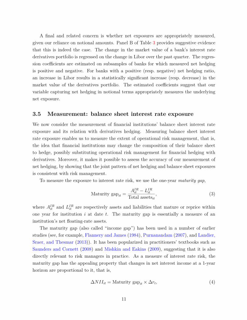
A final and related concern is whether net exposures are appropriately measured,given our reliance on notional amounts. Panel B of Table 3 provides suggestive evidencethat this is indeed the case. The change in the market value of a bank’s interest ratederivatives portfolio is regressed on the change in Libor over the past quarter. The regres-sion coefficients are estimated on subsamples of banks for which measured net hedgingis positive and negative. For banks with a positive (resp. negative) net hedging ratio,an increase in Libor results in a statistically significant increase (resp. decrease) in themarket value of the derivatives portfolio. The estimated coefficients suggest that ourvariable capturing net hedging in notional terms appropriately measures the underlyingnet exposure.

3.5 Measurement: balance sheet interest rate exposure

We now consider the measurement of financial institutions’ balance sheet interest rateexposure and its relation with derivatives hedging. Measuring balance sheet interestrate exposure enables us to measure the extent of operational risk management, that is,the idea that financial institutions may change the composition of their balance sheetto hedge, possibly substituting operational risk management for financial hedging withderivatives. Moreover, it makes it possible to assess the accuracy of our measurement ofnet hedging, by showing that the joint pattern of net hedging and balance sheet exposuresis consistent with risk management.

To measure the exposure to interest rate risk, we use the one-year maturity gap,

Maturity gapit = AIRit − LIRitTotal assetsit

, (3)

where AIRit and LIRit are respectively assets and liabilities that mature or reprice withinone year for institution i at date t. The maturity gap is essentially a measure of aninstitution’s net floating-rate assets.

The maturity gap (also called “income gap”) has been used in a number of earlierstudies (see, for example, Flannery and James (1984), Purnanandam (2007), and Landier,Sraer, and Thesmar (2013)). It has been popularized in practitioners’ textbooks such asSaunders and Cornett (2008) and Mishkin and Eakins (2009), suggesting that it is alsodirectly relevant to risk managers in practice. As a measure of interest rate risk, thematurity gap has the appealing property that changes in net interest income at a 1-yearhorizon are proportional to it, that is,

∆NIIit = Maturity gapit ×∆rt, (4)

11

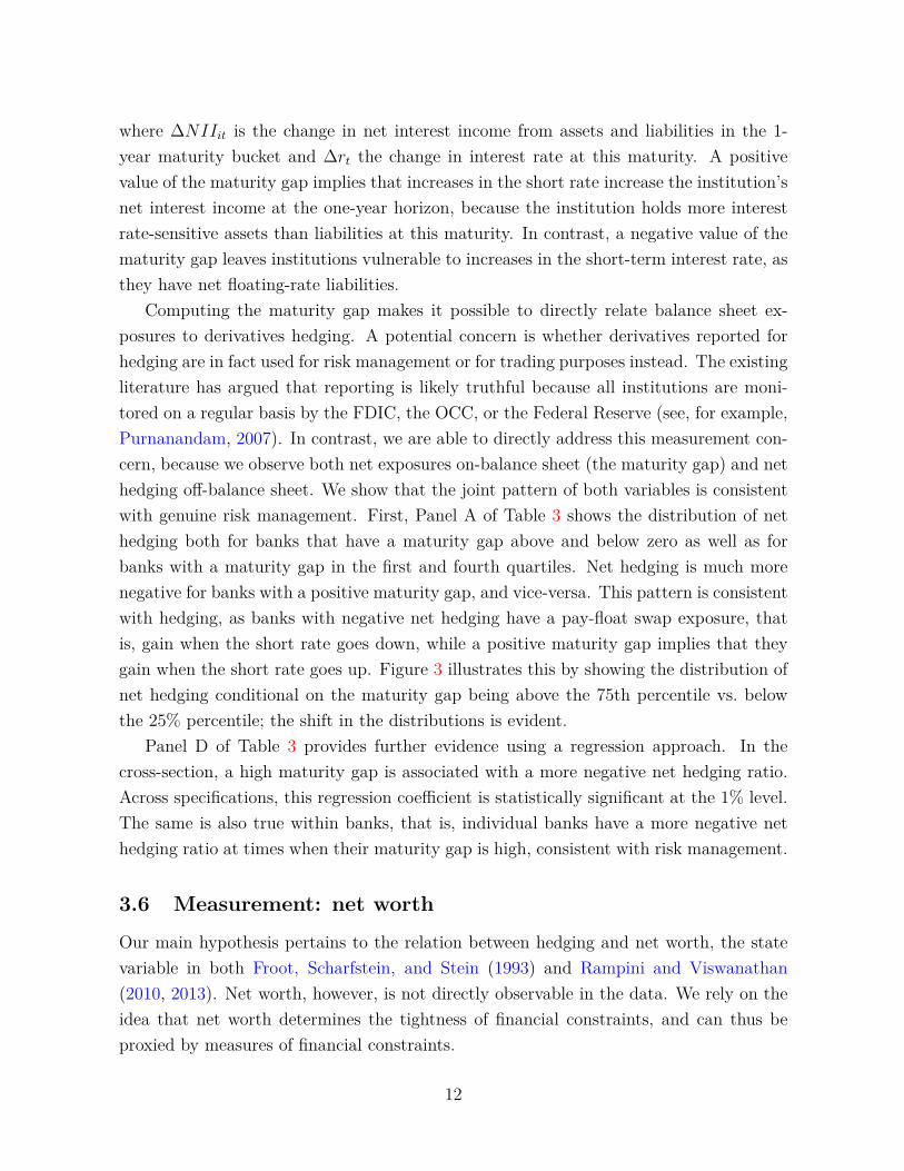
where ∆NIIit is the change in net interest income from assets and liabilities in the 1-year maturity bucket and ∆rt the change in interest rate at this maturity. A positivevalue of the maturity gap implies that increases in the short rate increase the institution’snet interest income at the one-year horizon, because the institution holds more interestrate-sensitive assets than liabilities at this maturity. In contrast, a negative value of thematurity gap leaves institutions vulnerable to increases in the short-term interest rate, asthey have net floating-rate liabilities.

Computing the maturity gap makes it possible to directly relate balance sheet ex-posures to derivatives hedging. A potential concern is whether derivatives reported forhedging are in fact used for risk management or for trading purposes instead. The existingliterature has argued that reporting is likely truthful because all institutions are moni-tored on a regular basis by the FDIC, the OCC, or the Federal Reserve (see, for example,Purnanandam, 2007). In contrast, we are able to directly address this measurement con-cern, because we observe both net exposures on-balance sheet (the maturity gap) and nethedging off-balance sheet. We show that the joint pattern of both variables is consistentwith genuine risk management. First, Panel A of Table 3 shows the distribution of nethedging both for banks that have a maturity gap above and below zero as well as forbanks with a maturity gap in the first and fourth quartiles. Net hedging is much morenegative for banks with a positive maturity gap, and vice-versa. This pattern is consistentwith hedging, as banks with negative net hedging have a pay-float swap exposure, thatis, gain when the short rate goes down, while a positive maturity gap implies that theygain when the short rate goes up. Figure 3 illustrates this by showing the distribution ofnet hedging conditional on the maturity gap being above the 75th percentile vs. belowthe 25% percentile; the shift in the distributions is evident.

Panel D of Table 3 provides further evidence using a regression approach. In thecross-section, a high maturity gap is associated with a more negative net hedging ratio.Across specifications, this regression coefficient is statistically significant at the 1% level.The same is also true within banks, that is, individual banks have a more negative nethedging ratio at times when their maturity gap is high, consistent with risk management.

3.6 Measurement: net worth

Our main hypothesis pertains to the relation between hedging and net worth, the statevariable in both Froot, Scharfstein, and Stein (1993) and Rampini and Viswanathan(2010, 2013). Net worth, however, is not directly observable in the data. We rely on theidea that net worth determines the tightness of financial constraints, and can thus beproxied by measures of financial constraints.

12

We use several measures of net worth. The first five are relatively standard and havebeen used by Rampini, Sufi, and Viswanathan (2014), among others; these are bookvalue of assets (“size”), market value of equity (“market capitalization”), market valueof equity to assets, net income to assets, and the credit rating. The sixth, a measureof cash dividends, has been used to measure financial constraints at least since Fazzari,Hubbard, and Petersen (1988). The last one is an index of net worth which we introduce.All variables are defined in more detail in Table 1.

Given the central role of net worth in our analysis, we construct a net worth indexas follows. We extract the first principal component of size, market value of equity toassets, net income to assets, and cash dividends to assets. The loadings on each of thesevariables are in Table 1. We exclude the rating variable in the construction of the indexto avoid being forced to exclude institutions for which no rating information is available.We think that this net worth index may be of independent interest.

The evolution of the cross-sectional distribution of each measure of net worth at thequarterly frequency is plotted in Figure 1. Notice the substantial drop in the marketvalue to assets, net income to assets, and dividends to assets during the financial crisis,and the corresponding drop in the net worth index we construct. Descriptive statisticsfor these variables are in Panel A of Table 5. Panel B of Table 5 shows the correlationbetween all measures of net worth. Interestingly, the net worth index is relatively lesscorrelated with size than with other variables such as the market value of equity to assets,net income, or cash dividends.

4 Hedging and net worth in cross section and timeseries

To study the determinants of risk management in financial institutions, we investigatethe relation between hedging and net worth, both in the cross-section and in the timeseries. We also examine the dynamics of hedging for institutions approaching distress.

4.1 Hedging and net worth across financial institutions

We provide evidence of a positive cross-sectional relation between interest rate hedgingand net worth at the BHC level. To isolate cross-sectional variation, we estimate BHC-mean specifications, where both dependent and independent variables are averaged foreach BHC over the sample period. We also estimate a pooled OLS specification with timefixed effects, to control for time trends in hedging. The results are reported in Panel A of

13

Table 6. In both specifications, the estimated coefficients are positive and significant atthe 1% level (and in one case at the 5% level) for six out of seven measures of net worth.The magnitude of the effect is economically relevant. Focusing on BHC-mean estimates,one standard deviation increase in size is associated with an increase in hedging equal to53% of a standard deviation. For other measures, a one-standard deviation increase inthe credit rating (resp. the net worth index) is associated with an increase in hedging by25% (resp. 23%) of a standard deviation.

One concern with the above specifications is the large number of zeros in the dependentvariable (49% in the BHC sample), possibly biasing estimates downwards. Indeed, forBHCs that do not hedge, variation in net worth does not translate to any variation inhedging. We turn to several estimation methods which account for the fact that hedginghas a mass point at zero. We estimate (i) a BHC-mean Tobit, where both the dependentand independent variables are averaged for each BHC over all periods, before a Tobitspecification is estimated, (ii) a Tobit specification in the pooled sample, with time fixedeffects, (iii) quantile regressions in the upper percentiles (75th, 85th and 95th) of thedistribution of gross hedging, and (iv) a Heckman selection model. In the first stage ofthe Heckman estimation, we predict whether a BHC hedges or not using the net worthindex and size (orthogonalized on the net worth index) to capture the potential effect offixed costs on the participation decision. In the second stage, the magnitude of hedgingis predicted using the net worth index.

Estimates for these specifications are in Panel B of Table 6. With two exceptions,estimated coefficients are all positive and significant at the 1% level.16 The fact thathedging drops as net worth declines is also seen from regressions of hedging on creditrating dummies reported in Panel C of Table 6. Estimates are given as differences withrespect to the hedging level by institutions in a bucket from A- to AAA. Institutionswith low credit ratings hedge significantly less than institutions with high credit ratingsin the cross-section. Overall, these results suggest that, in the cross-section, financialinstitutions with high net worth hedge more than institutions with low net worth. Incontrast to previous work, we emphasize that cross-sectional patterns in hedging are notmainly driven by size, but by net worth, proxied by several measures.17

16We report only the estimate from the second stage of the Heckman estimation; in the first stage,both the net worth index and size, orthogonalized on the net worth index, are statistically significant.

17We obtain similar results at the bank-level, with net worth measured by size, net income, anddividends, but do not report these findings here.

14

4.2 Hedging and net worth within financial institutions

We now turn to the panel dimension and use institution fixed effects to isolate within-institution variation in hedging. The inclusion of fixed effects serves two purposes. First, itis meant to provide more stringent evidence of the positive relation between net worth andhedging. Our hypothesis is that, over time, financial institutions hedge more when theyare better capitalized and cut hedging when they become more constrained. Second, fixedeffects make it possible to difference out any time-invariant unobserved heterogeneity, suchas differences in business models, sophistication, or the fixed costs of setting up a hedgingdesk, which may affect estimates in pooled regressions.

Results for all fixed effect regressions are in Table 7. Panel A provides estimates atthe BHC level, and Panels B and C at the bank level, focusing on gross and net hedging,respectively. In all cases, the fixed effect estimates in the whole sample are either positiveand significant or insignificant. The economic magnitude of the effect is attenuated withrespect to the cross-sectional regressions, but is still appreciable. Since theory predictsthat the trade-off between hedging and financing is more acute for banks with low networth, we provide an additional specification by excluding the 10% of institutions withthe highest net worth. When these institutions are excluded (see the second specificationin Panel A), all coefficients are positive and significant at the 1% level.

Further, we estimate two additional specifications to account for the large number ofzeros. We estimate a regression with BHC fixed effects excluding all institutions whichnever use derivatives. We also use the trimmed least absolute deviations estimator pro-posed by Honoré (1992), which makes it possible to estimate a model with fixed effectsin the presence of truncated data. In both cases, all significant coefficients are positive,although in the latter specification, only two of seven coefficients are significant. Finally,at the bank level, we find positive and significant effects for all three measures of networth available for gross hedging, and for two of the three variables available for theabsolute value of net hedging. That said, the magnitude of the effects at the bank levelis smaller.

To sum up, we find a statistically significant and economically appreciable positiverelation between hedging and net worth within financial institutions, corroborating ourcross-sectional results.

4.3 Hedging before distress

We provide additional evidence of the relation between hedging and net worth withininstitutions by focusing on hedging by institutions that enter financial distress and thus

15

become severely constrained.18

We define a distress event for a BHC (resp. a bank) as any exit from the sample witha ratio of market capitalization (resp. common equity) to total assets below 4% in the lastquarter in which the institution is in the sample.19 Restricting attention to institutionswhich exit the sample with a market capitalization or common equity below 4% of totalassets ensures that these institutions are distressed. We identify all such distress eventsover the sample period and restrict the sample to BHCs and banks which hedge in at leastone quarter. There are 49 distress events for BHCs and 636 distress events for banks. Ofthese events, 95.9% involve mergers or purchases before the entity actually fails, and theothers are failures in which FDIC assistance is provided.

We use a regression approach to investigate the extent of hedging in the eight quartersbefore distress. We estimate

Hedgingit = FEi + FEt +8∑j=0

γj ·Dτ−j + εit, (5)

where τ is the quarter in which institution i exits the sample in distress andDτ−j a dummyvariable that equals 1 for distressed institutions at each date τ − j ∈ {τ − 8, ..., τ} and 0otherwise. The specification includes institution fixed effects (FEi) and time fixed effects(FEt), to isolate within-institution variation before distress.

Equation (5) is estimated both at the BHC and the bank level, using the whole sampleof distressed and non-distressed institutions. At the bank level, we estimate it for bothgross and net hedging. Regression coefficients are collected in Table 8. Both gross andnet hedging decrease by a statistically significant amount several quarters before distress.Interestingly, both are reduced by comparable amounts at the bank level, again suggestingthat gross and net hedging are relatively similar for most banks.

The economic magnitude of the pre-distress reduction in hedging is large. Financialinstitutions cut hedging by close to one half. Figure 4 illustrates this result by plottingmean and median hedging before distress for institutions for which all 8 observations

18While we focus on hedging before distress here, we emphasize that the positive relation betweenhedging and net worth is not just due to financial institutions that are close to distress. In fact, we obtainvery similar results in our cross-sectional and within regressions after dropping the 10% of observationswith the lowest net worth (as measured by the pertinent variable for each regression).

19There are several reasons why financial institutions exit the sample, including mergers and acquisi-tions or failures. The reason for exiting the sample is obtained from the National Information Center(NIC) transformation data. Distinguishing between actual failures and distress episodes leading to ac-quisitions is, however, of limited interest for our purposes. Mergers and acquisitions are indeed oftenarranged before FDIC assistance is provided and the bank actually fails (see Granja, Matvos, and Seru,2014).

16

before exit are available. In all cases, approaching distress is associated with a reductionof both mean and median hedging. For banks, median hedging falls to zero at the timeof exit. Both the regression results and the figures are strongly suggestive of the factthat, as institutions become more constrained, the opportunity cost of hedging becomestoo large. Cutting hedging for such institutions is the optimal response in the face ofmore severe financing constraints. Since institutions cut hedging so dramatically beforedistress, one might be tempted to conclude that these cuts are explained by risk shiftingbefore distress. We discuss this alternative hypothesis in Section 6. To anticipate ourconclusion, we provide evidence on the trading behavior of these institutions that suggeststhat risk shifting is not a plausible interpretation of these findings.

5 Identification using house pricesWe turn to our identification strategy next. We use changes in house prices to assess theeffect of variation in net worth on hedging. First, we instrument net income with changesin local house prices. Second, we estimate the effect of a drop in net worth on hedgingusing a difference-in-differences estimation.

5.1 Instrumenting net income with changes in house prices

We use local house prices to instrument for net income, a key component of the change innet worth. We exploit the fact that, over the period from 2005 to 2013, changes in financialinstitutions’ net income are driven to an important extent by losses on loans secured byreal estate, which are in turn driven by variation in house prices. We instrument netincome by lagged changes in house prices at the local level. Because the instrument islikely stronger for institutions with a high exposure to real estate, we restrict attentionto institutions with a ratio of loans secured by real estate to assets above the samplemedian.

Our identifying assumption is that house prices affect hedging only through their im-pact on financial institutions’ net worth, as proxied by net income. We start by providingsupporting evidence in favor of this instrument. First, we show that changes in net incomeover the 2005-2013 period arise to a large extent from provisions for loan losses causedby drops in house prices. Second, we address a potential endogeneity concern by showingthat changes in net income over the period do not also arise to a significant extent –directly or indirectly through defaults on mortgages – from changes in interest rates.

We first conduct a variance decomposition of changes in net income. Net income can

17

be written as

Net incomeit = Net interest incomeit +Net noninterest incomeit−Provisionsit + εit, (6)

where εit contains extraordinary items, income taxes, and income attributable to non-controlling (minority) interests. We use a regression approach to decompose changes innet income into changes in its three main components. The results of this decompositionare provided in Table 9, in which t-statistics are reported together with the regressioncoefficients. Two features are worth noting. First, as can be seen in columns (1) and (4),changes in net income arise to a large extent from provisions for loan losses. Second, asseen in column (2), variation in net interest income is not a significant driver of changes innet income over the period. Thus we can rule out the concern that changes in net worth,as measured by net income, may be driven to a significant extent by interest rates, as thedecomposition shows that this concern is not warranted.20 Figure 5 provides a graphicalillustration of the decomposition; notice that while the variation of net interest incomeover time is limited, provisions increase massively exactly at the time when net incomedrops dramatically.

Turning to provisions for loan losses, the fourth panel in Figure 5 shows that provisionsincrease primarily to face losses on loans secured by real estate. Over the sample period,nonaccrual real estate loans represent the vast majority of total nonaccrual loans. For ourinstrument to be valid, however, two additional steps are needed. First, it has to be thecase that changes in house prices drive defaults on loans secured by real estate, primarilymortgages, to a significant extent. Second, an additional endogeneity concern must beaddressed. If defaults on loans secured by real estate are importantly related to changes inthe interest rate environment, then such changes may also affect the incentive to engage ininterest rate hedging, for reasons unrelated to net worth. To address these two concerns,we turn to the sizeable literature which studies mortgage defaults over our sample period.This literature largely concludes that house prices were the main driver of mortgagedefaults from 2007 onwards (see, for example, Bajari, Chu, and Park (2008), Mayer,Pence, and Sherlund (2009), Demyanyk and Van Hemert (2011), and Palmer (2014)).Second, a number of these papers also stress that the interest rate environment played aminor role in explaining mortgage defaults. Importantly, the interest rate environmentwas the same across the U.S., while there was a lot of local heterogeneity in mortgagedefaults, driven by local heterogeneity in house prices drops. These findings suggest thatour instrument is valid and satisfies exogeneity conditions.

20The other important component of changes in net income is changes in non-interest income. Un-reported results show that these changes are almost entirely attributable to goodwill impairments of asmall subset of banks. For other banks, changes in provisions explain the bulk of changes in net income.

18

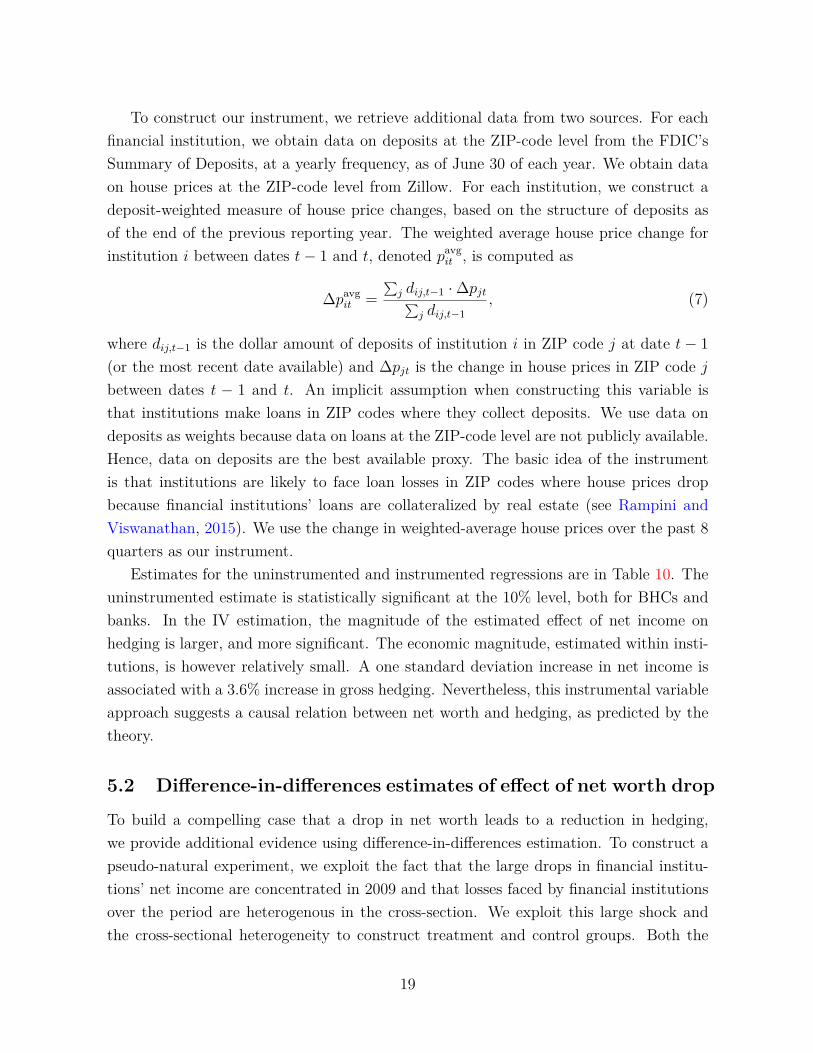
To construct our instrument, we retrieve additional data from two sources. For eachfinancial institution, we obtain data on deposits at the ZIP-code level from the FDIC’sSummary of Deposits, at a yearly frequency, as of June 30 of each year. We obtain dataon house prices at the ZIP-code level from Zillow. For each institution, we construct adeposit-weighted measure of house price changes, based on the structure of deposits asof the end of the previous reporting year. The weighted average house price change forinstitution i between dates t− 1 and t, denoted pavg

it , is computed as

∆pavgit =

∑j dij,t−1 ·∆pjt∑

j dij,t−1, (7)

where dij,t−1 is the dollar amount of deposits of institution i in ZIP code j at date t− 1(or the most recent date available) and ∆pjt is the change in house prices in ZIP code jbetween dates t − 1 and t. An implicit assumption when constructing this variable isthat institutions make loans in ZIP codes where they collect deposits. We use data ondeposits as weights because data on loans at the ZIP-code level are not publicly available.Hence, data on deposits are the best available proxy. The basic idea of the instrumentis that institutions are likely to face loan losses in ZIP codes where house prices dropbecause financial institutions’ loans are collateralized by real estate (see Rampini andViswanathan, 2015). We use the change in weighted-average house prices over the past 8quarters as our instrument.

Estimates for the uninstrumented and instrumented regressions are in Table 10. Theuninstrumented estimate is statistically significant at the 10% level, both for BHCs andbanks. In the IV estimation, the magnitude of the estimated effect of net income onhedging is larger, and more significant. The economic magnitude, estimated within insti-tutions, is however relatively small. A one standard deviation increase in net income isassociated with a 3.6% increase in gross hedging. Nevertheless, this instrumental variableapproach suggests a causal relation between net worth and hedging, as predicted by thetheory.

5.2 Difference-in-differences estimates of effect of net worth drop

To build a compelling case that a drop in net worth leads to a reduction in hedging,we provide additional evidence using difference-in-differences estimation. To construct apseudo-natural experiment, we exploit the fact that the large drops in financial institu-tions’ net income are concentrated in 2009 and that losses faced by financial institutionsover the period are heterogenous in the cross-section. We exploit this large shock andthe cross-sectional heterogeneity to construct treatment and control groups. Both the

19

concentration of losses and the cross-sectional heterogeneity are apparent in the top leftpanel of Figure 5, where the year 2009, which we use to define our treatment, is shaded.

As before, we restrict attention to financial institutions with a high exposure to realestate, defined by a ratio of loans secured by real estate to total assets above the samplemedian in 2008Q4. Among these institutions with a high exposure to real estate, we definethe treatment group as institutions in the bottom 30% of the net income distribution in2009. These institutions have negative net income, that is, face losses which decreasetheir net worth. We define the control group as institutions in the top 30% of the netincome distribution in that year. These institutions have positive net income on average.The event date is defined as of 2009, and we focus on a 4-year window before and afterthe event, that is, 2005 to 2013. We drop institutions which exit the sample over thisperiod. We further restrict the sample to institutions which have strictly positive hedgingin at least one quarter before the event. The fact that we restrict attention to institutionswith a high exposure to real estate ensures that both treatment and control groups havea similar potential to face losses on real estate loans ex ante. Theory predicts thatinstitutions in the treatment group cut hedging more than institutions in the controlgroup.

We estimate three main specifications. In the first, we include a dummy variable thattakes value one for treated banks after the treatment. In the other two specifications,we include treatment-year dummies for each year after the treatment, without and withinstitution fixed effects. Estimates are reported in Columns (1) to (3) in Table 11, inPanel A for BHCs and in Panel B for banks. There is a statistically significant drop inhedging by institutions in the treatment group relative to the control institutions. Thisis true for both BHCs and banks. Furthermore, the magnitude is economically large.Both treated BHCs and banks cut hedging by about one half in the post-2009 period,relative to the control group. Furthermore, the drop in net worth has persistent effects,as hedging by treated institutions does not recover to its pre-2009 level relative to controlinstitutions. These effects are illustrated at the BHC level in Figure 6.

Changes in net income in 2009 are arguably exogenous to the interest rate environ-ment, implying that financial institutions which cut hedging after the event do so becausetheir net worth is lower, not because the incentive to engage in interest rate risk man-agement has changed due to the change in interest rates. To nevertheless address anyfurther endogeneity concerns, we consider two alternative treatments that are further re-moved from financial institutions’ decisions. We continue to restrict attention to financialinstitutions with a ratio of loans secured by real estate over total assets above the samplemedian.

20

First, for each institution, we compute a deposit-weighted measure of the change inhouse prices over the period from 2007Q1 to 2008Q4, as described earlier. This measureuses data on deposits and house prices at the ZIP-code level. We define the treatmentgroup as institutions in the bottom 30% of weighted-average house price changes. Theseinstitutions face large drops in local house prices in the two years leading up to 2009. Incontrast, we define the control group as institutions in the top 30% of house price changes.Among institutions with ex ante similar exposure to real estate, treated institutions arethose which face relatively large drops in local house prices. The interpretation of thispseudo-natural experiment is that such drops affect financial institutions’ net worth forreasons unrelated to interest rates, as the interest rate environment is the same for thetreatment and control group.

Second, we also compute, for each institution, a measure of the housing supply elastic-ity at a local level, namely the deposit-weighted average housing supply elasticity. To doso, we obtain data on the housing supply elasticity at the Metropolitan Statistical Area(MSA) level from Saiz (2010). This measure, available for 269 MSAs, is constructed usingsatellite-generated data on terrain elevation and on the presence of water bodies. It ismatched with deposit data at the MSA level and used to construct an institution-specificdeposit-weighted measure of housing supply elasticity, εavg

i , as

εavgi =

∑j dij · εj∑j dij

, (8)

where εj is the housing supply elasticity in MSA j, and dij is the stock of deposits of in-stitution i in MSA j, measured in 2008.21 We define the treatment group as institutionsin the bottom 30% of deposit-weighted average housing supply elasticity. These insti-tutions are more likely to face large house prices drops. We define the control group asinstitutions in the top 30% of housing supply elasticity. The interpretation of this pseudo-natural experiment is that areas in which the housing supply is inelastic are subject tolarger house price fluctuations, which may in turn affect the net worth of institutions thatare highly exposed to the housing sector. Moreover, housing supply elasticity is unrelatedto the interest rate environment.

We estimate the same three specifications as we did with net income before for eachof these two alternative definitions of the treatment and control groups. Estimates arereported in Columns (4) to (9) in Table 11. The results are consistent with those of thebaseline specification and statistically significant, except at the bank-level when treatmentis based on local housing supply elasticity. Institutions which face a larger decline in local

21The housing supply elasticity measure provided by Saiz (2010) is purely cross-sectional, that is, thereis no within-MSA time variation that can be exploited.

21

house prices or a lower local housing supply elasticity cut hedging significantly more thaninstitutions in the relevant control groups. The magnitude of the estimated effect is largeand economically substantial, as with the baseline specification. When the treatment isbased on house price changes, treated institutions, both BHCs and banks, cut hedging bymore than one half. When the treatment is based on the local housing supply elasticity,the estimated coefficient and hence economic magnitude of the effect is even larger. Inpart, this is due to the fact that not all institutions can be matched with the data by Saiz(2010), as this data is available for 269 MSAs only. The sample size is lower, and hedgingbefore treatment is higher for both the treatment and the control groups in this case.Relative to the pre-treatment level, the estimated magnitude of the effect is comparableto that estimated with other definitions of the treatment.

To sum up, our difference-in-difference estimates imply that financial institutionswhose net worth drops in 2009 relative to an otherwise similar control group cut hedgingsubstantially. The effect of the drop in net worth on hedging is not just statisticallysignificant but also economically sizeable; indeed, the drop in net worth leads financialinstitutions to cut their hedging by about half. We obtain similar estimates whether wedefine the treatment directly in terms of the drop in net income or in terms of the dropin local weighted-average house prices or weighted-average housing supply elasticity.

5.3 Robustness – pre-trends and maturity gap

We now discuss the robustness of our difference-in-differences estimation. First, we pro-vide evidence supporting the parallel trends assumption. Second, we show that financialinstitutions’ balance sheet exposure to interest rate risk behaves similarly in the treatmentand in the control groups over the sample period.

The parallel trends assumption is the identifying assumption in difference-in-differencesestimation. Trends in the outcome variable must be the same in the treatment and inthe control group before the treatment. This assumption cannot be formally tested. In-stead, we provide supporting evidence by including treatment-year dummies during thepre-treatment period in our benchmark specification. Such estimates, along with post-treatment dummies, are reported in Panel A of Table 12. These estimates, both withoutand with institution fixed effects, show that there are no significant differences in trendsbetween treatment and control groups during the pre-treatment years, and that hedgingin the treatment and control group diverge significantly only from 2009 onwards. Thefact that trends in hedging are parallel in the treatment and the control group before2009 in our benchmark specification can also be seen graphically in Figure 6. Thus, thekey identifying assumption seems valid.

22

Another potential concern is that financial institutions’ balance sheet exposure tointerest rate risk in the treatment and the control group changes differentially after thetreatment. If treated and control institutions are left with different hedgeable exposures,they may be induced to adjust derivatives hedging differentially not because their networth changes, but because the exposures change. This concern is not warranted. Toshow this, we rerun our main difference-in-differences specification, replacing hedging bythe maturity gap as the dependent variable. Estimates are in Panel B of Table 12. Withthe exception of the year 2009, the differences in the maturity gap between the treatmentand control groups are never statistically different after the treatment. The fact thatthe maturity gap in both groups evolves very similarly around the treatment can alsobe seen visually in Figure 7. The only statistically significant difference that appears,in 2009 (that is, in the treatment year), contradicts the idea that BHCs which reducederivatives hedging have also reduced their operational risk exposure. These institutionsinstead choose a more negative maturity gap, that is, if anything, increase their exposureto interest rate risk by taking on more pay-floating liabilities. We discuss the dynamicsof the maturity gap in more detail in Section 6.2.

We conclude that there are no differential trends between the treatment and controlgroup before the treatment and that the balance sheet interest rate risk exposures do notevolve differentially in the two groups either before or after the treatment. Hence, ourdifference-in-differences strategy identifies a negative causal effect of drops in financialinstitutions’ net worth on hedging.

6 Alternative hypothesesSo far, we have emphasized financial constraints as the main determinant of the positiverelation between hedging and net worth. We now consider alternative explanations thatmight be consistent with this positive relation. Specifically, we first study whether thereduction in risk management by financially constrained institutions is evidence of riskshifting. Next we consider whether institutions that reduce financial hedging increaseoperational hedging by adjusting the maturity structure of their balance sheet instead.Finally, we ask whether the determinant of hedging is financial institutions’ regulatorycapital rather than their market net worth. None of these three alternative hypothesesare supported by the data.

23

6.1 Risk shifting? Evidence from trading

An alternative explanation for the positive relation between hedging and net worth is riskshifting resulting from an agency conflict between debtholders and shareholders. Due tolimited liability, the payoffs of equity holders around distress are convex, so that theymay benefit from an increase in the volatility of net income (see Jensen and Meckling,1976). This may induce them to reduce hedging (see, for example, Leland, 1998).

We provide evidence inconsistent with risk shifting. We rely on the idea that, iffinancial institutions engage in risk shifting in derivatives markets, they should reducehedging, but they should also increase trading. In contrast, if financial constraints are themain reason why institutions reduce hedging, as the theory we test in this paper suggests,then no such increase is predicted. In contrast, institutions might reduce trading as well,if trading also requires net worth. Both theories provide similar predictions with respectto hedging, but make differing predictions about trading. We test these predictions byfocusing on financial institutions’ portfolio of derivatives for trading purposes.22

In Panel A of Table 13, we study the relation between trading and net worth. The firsttwo specifications, a BHC-mean Tobit and a pooled Tobit, exploit cross-sectional variationin trading. For all measures of net worth, BHCs with higher net worth trade more, notless, and the relation is statistically significant in most cases. The third specificationisolates within-BHC variation in net worth, and speaks thus more directly to the risk-shifting hypothesis. Again, there is a positive and significant relation between trading andnet worth. Financial institutions trade more not when their net worth is low, but whenit is high. This evidence is at odds with risk shifting and consistent with the existence offinancial constraints.

Furthermore, because risk shifting is more of a concern around distress, we studythe trading behavior of financial institutions entering distress, defined as in Section 4.3.Panel B of Table 13 analyzes gross trading before distress for institutions that exit thesample using dummies for up to eight quarters before distress. BHCs cut trading bya statistically significant amount before distress. At the bank level, coefficients are notstatistically significant. Trading by banks before distress is plotted in Panel A of Figure 8.Mean trading drops before distress. Again, this is the opposite of what risk shifting wouldpredict.

It is moreover worth noting that we find a positive relation between hedging and networth not just for institutions in distress but in our data overall.23 And we do not find

22Recall that we exclude the six main broker-dealers in the results we report which is warranted fortrading because most of the trading activities of these dealers arise from market making.

23Indeed, one reason why it is not plausible that the basic pattern is due to risk shifting is that we find

24

discontinuous hedging behavior as net worth drops. This smooth behavior of hedging isin marked contrast to the discontinuous behavior predicted by models of risk shifting.Together, these results suggest that financial constraints, not risk shifting, explain thepositive relation between risk management and net worth. The results are also consistentwith empirical evidence in other sectors (see Andrade and Kaplan (1998) for highly lever-aged transactions and Rauh (2009) for corporate pension plans), according to which riskmanagement concerns dominate risk shifting incentives even in the vicinity of bankruptcy.

6.2 Operational risk management

Another concern might be that financial institutions which have lower net worth cutfinancial hedging, but substitute it with operational risk management, that is, reducetheir on-balance sheet exposure to interest rate risk (see Petersen and Thiagarajan (2000)and Purnanandam (2007)). We investigate this alternative hypothesis by studying therelation between financial institutions’ maturity gap and their net worth. The evidenceis not consistent with this alternative hypothesis.

Panel A of Table 14 provides evidence of a positive and significant relation betweenthe maturity gap and net worth. Financial institutions with higher net worth have morenet floating-rate assets than institutions with low net worth. If anything, they do moreoperational risk management, while at the same time hedging more using derivatives. Thisevidence suggests that financial institutions with low net worth engage less in any typeof risk management, either on-balance sheet or off-balance sheet. The fact that any typeof risk management is more costly for such institutions is consistent with the theoreticalpredictions by Rampini and Viswanathan (2010, 2013) and broadly inconsistent with theidea that operational risk management is used as a substitute for derivatives hedging.

Additional evidence against operational risk management is obtained by focusing onfinancial institutions that approach distress. Operational risk management would implythat these institutions hold more net-floating rate assets, that is, that their maturitygap increases as they approach distress. Panel B of Table 14 reports the results ofregressions of the maturity gap on a set of dummies that take value one up to eightquarters before distress for both BHCs and banks that exit the sample. The maturitygap of such institutions gets more negative as they approach distress, and the drop isstatistically significant several quarters before they exit. These institutions thus do lessoperational risk management as they become more constrained, as also illustrated in

the same positive relation between hedging and net worth in our cross-sectional and within regressionseven after dropping the 10% of observations with the lowest net worth (see footnote 18), whereas riskshifting might predict such a pattern close to distress but not otherwise.

25

Panel B of Figure 8. Quantitatively, the drop is remarkably large, exceeding 10% ofassets for both banks and BHCs. This pattern, which to the best of our knowledge hasnot been documented before, is of independent interest.

Overall, these results suggest that operational risk management cannot provide a sat-isfactory explanation for the positive relation between net worth and hedging. We find aremarkably strong pattern going the opposite way, as more financially constrained finan-cial institutions have more net floating-rate liabilities, not less. The existence of financialconstraints is consistent with the fact that operational risk management is reduced, notincreased, as financial institutions become more constrained.

6.3 Regulatory capital versus net worth

Another alternative explanation is that the positive relation between hedging and networth is driven not by market measures of net worth, which we use, but by regulatorycapital. This could be the case, for example, if counterparties in the swap market payattention not to market net worth but to regulatory capital. If so, the positive relationwhich we document might spuriously arise from the positive correlation between marketmeasures of net worth and regulatory capital. At the same time, if regulators monitor thehedging policies of financial institutions, they might in fact require more hedging whenregulatory capital is lower, not higher. If this were the dominant force, then one wouldexpect a negative relation between hedging and regulatory capital.

To investigate its role, we estimate the relation between hedging and two measuresof regulatory capital for BHCs. We use both total regulatory capital and Tier 1 capital,normalized by risk-weighted assets. Panel A of Table 15, provides the estimates of fourregression specifications, which exploit both the cross-sectional and the within-institutionvariation in regulatory capital. None of the estimated coefficients, except one, are sta-tistically significant. There is no significant and stable relation between hedging andregulatory capital, neither between institutions nor within institutions.

We further conduct the J-test proposed by Davidson and MacKinnon (1981) to testthe specification with our (market-based) measures of net worth against the alternativespecification with regulatory capital. The residuals of the regression of hedging on regu-latory capital are regressed on our market-based measures of net worth. Because tests ofmodel specification have no natural null hypothesis (see, for example, Greene, 2012), wealso regress the residuals of the models with our market-based measures of net worth onregulatory capital. Panel B in Table 15 reports t-statistics for the second stage regres-sion of the test. The hypothesis that the model with regulatory capital is true is alwaysrejected in favor of our specification with market-based net worth. When we reverse the

26

order of the hypotheses, we find that our model with market-based net worth is typicallynot rejected in favor of the alternative hypothesis with regulatory capital.

Together with the above regression results, this test provides strong suggestive ev-idence against regulatory capital being a major determinant of hedging. The primarydeterminant of the hedging behavior of financial institutions seems to be their net worth,not their regulatory capital. The emphasis on regulatory capital as a determinant of fi-nancial institutions’ risk exposures in much of the literature and policy debate may hencenot be warranted.

7 ConclusionThe evidence that we present strongly suggest that the financing needs associated withhedging are a substantial barrier to risk management for financial institutions. Consistentwith the theoretical predictions of Rampini and Viswanathan (2010, 2013), we find astrong positive relation between interest rate hedging and net worth across financialinstitutions and within institutions over time; better capitalized financial institutionshedge more. We use a novel identification strategy based on shocks to the net worth offinancial institutions due to drops in house prices. This allows us to conclude that suchdrops in net worth lead to a reduction in hedging.

We provide auxiliary evidence that is inconsistent with alternative hypotheses. Thereis a strong positive relation between trading and net worth which goes against the ideathat more constrained financial institutions engage in risk shifting by trading more. More-over, there is a strong positive relation between the maturity gap and net worth which goesagainst the idea that more constrained financial institutions substitute financial hedgingwith operational risk management. We do not observe a strong relation between hedgingand regulatory capital, and model comparison tests suggest that it is market measures ofnet worth rather than regulatory capital that explain the hedging behavior of financialinstitutions.

We contend that financial constraints are a key impediment to risk management byfinancial institutions and firms, and to insurance by households, and result in financial in-stitutions, firms, and households being more exposed to tradeable or insurable risks thanthey otherwise would be. The implications of our findings for the dynamics of financingand investment by institutions and households and the consequences for macroeconomicactivity may be significant. Limited interest rate risk management leaves financial in-stitutions, especially financially constrained ones, exposed to changes in interest rates,which is an essential fact for both monetary and macro-prudential policy to consider.

27

ReferencesAdelino, M., A. Schoar, and F. Severino (2015). House prices, collateral and self-employment. Journal of Financial Economics 117, 288–306.

Andrade, G. and S. N. Kaplan (1998). How costly is financial (not economic) distress?Evidence from highly leveraged transactions that became distressed. Journal of Fi-nance 53, 1443–1493.

Avraham, D., P. Selvaggi, and J. Vickery (2012). A structural view of U.S. bank holdingcompanies. FRBNY Economic Policy Review June, 65–81.

Bajari, P., C. S. Chu, and M. Park (2008). An empirical model of subprime mortgagedefault from 2000 to 2007. NBER Working Paper 14625 .

Begenau, J., M. Piazzesi, and M. Schneider (2015). Banks’ risk exposures. Working paper .

Bernanke, B. and M. Gertler (1989). Agency costs, net worth and business fluctuations.American Economic Review 79, 14–31.

Bernanke, B. and M. Gertler (1995). Inside the black box: The credit channel of monetarypolicy transmission. Journal of Economic Perspectives 9, 27–48.

Bord, V. M., V. Ivashina, and R. D. Taliaferro (2014). Large banks and the transmissionof financial shocks. Working Paper .

Breeden, D. and S. Viswanathan (1998). Why do firms hedge? An asymmetric informa-tion model. Working Paper .

Brunnermeier, M. K. and Y. Sannikov (2014). A macroeconomic model with a financialsector. American Economic Review 104, 379–421.

Campello, M. (2002). Internal capital markets in financial conglomerates: Evidence fromsmall bank responses to monetary policy. Journal of Finance 57, 2773–2805.

Chaney, T., D. Sraer, and D. Thesmar (2012). The collateral channel: How real estateshocks affect corporate investment. American Economic Review 102, 2381–2409.

Chernenko, S. and M. Faulkender (2011). The two sides of derivatives usage: Hedging andspeculating with interest rate swaps. Journal of Financial and Quantitative Analysis 46,1727–1754.

Chodorow-Reich, G. (2014). The employment effects of credit market disruptions: Firm-level evidence from the 2008-9 financial crisis. Quarterly Journal of Economics 129,1–59.

Cuñat, V., D. Cvijanović, and K. Yuan (2014). Within bank transmission of real estateshocks. Working Paper .

28

Davidson, R. and J. G. MacKinnon (1981). Several tests for model specification in thepresence of alternative hypotheses. Econometrica 49, 781–793.

DeMarzo, P. and D. Duffie (1995). Corporate incentives for hedging and hedge accounting.Review of Financial Studies 8, 743–777.

Demyanyk, Y. and O. Van Hemert (2011). Understanding the subprime mortgage crisis.Review of Financial Studies 24, 1848–1880.

Ellul, A. and V. Yerramilli (2013). Stronger risk controls lower risk: Evidence from U.S.bank holding companies. Journal of Finance 68, 1757–1803.

Fazzari, S. M., R. G. Hubbard, and B. C. Petersen (1988). Financing constraints andcorporate investment. Brookings Paper on Economic Activity 1, 141–195.

Flannery, M. J. and C. M. James (1984). The effect of interest rate changes on thecommon stock returns of financial institutions. Journal of Finance 39, 1141–1153.

Froot, K. A., D. S. Scharfstein, and J. C. Stein (1993). Risk management: Coordinatingcorporate investment and financing policies. Journal of Finance 48, 1629–1658.

Froot, K. A. and J. C. Stein (1998). Risk management, capital budgeting and capitalstructure policy for financial institutions: An integrated approach. Journal of FinancialEconomics 47, 55–82.

Géczy, C., B. A. Minton, and C. Schrand (1997). Why firms use currency derivatives.Journal of Finance 52, 1323–1354.

Gertler, M. and S. Gilchrist (1994). Monetary policy, business cycles, and the behaviorof small manufacturing firms. Quarterly Journal of Economics 109, 309–340.

Gertler, M. and N. Kiyotaki (2010). Financial intermediation and credit policy in businesscycle analysis. In B. M. Friedman and M. Woodford (Eds.), Handbook of MonetaryEconomics, pp. 547–599. Elsevier.

Granja, J., G. Matvos, and A. Seru (2014). Selling failed banks. Working Paper .

Greene, W. H. (2012). Econometric Analysis (7th ed.). Pearson.

Guay, W. and S. Kothari (2003). How much do firms hedge with derivatives? Journal ofFinancial Economics 70, 423–461.

Holmström, B. and J. Tirole (1997). Financial intermediation, loanable funds, and thereal sector. Quarterly Journal of Economics 112, 663–691.

Holmström, B. and J. Tirole (2000). Liquidity and risk management. Journal of MoneyCredit and Banking 32, 295–319.

29

Honoré, B. (1992). Trimmed LAD and least squares estimation of truncated and censoredregression models with fixed effects. Econometrica 60, 533–565.

Jensen, M. and W. Meckling (1976). Theory of the firm: Managerial behavior, agencycosts and ownership structure. Journal of Financial Economics 3, 305–360.

Jiménez, G., S. Ongena, J.-L. Peydró, and J. Saurina (2012). Credit supply and monetarypolicy: Identifying the bank balance-sheet channel with loan applications. AmericanEconomic Review 102, 2301–2326.

Kashyap, A. K. and J. C. Stein (2000). What do a million observations on banks sayabout the transmission of monetary policy? American Economic Review 90, 407–428.

Kleiner, K. (2015). House price contagion: Evidence from bank branching networks.Working Paper .

Landier, A., D. Sraer, and D. Thesmar (2013). Banks’ exposure to interest rate risk andthe transmission of monetary policy. Working paper .

Leland, H. E. (1998). Agency costs, risk management, and capital structure. Journal ofFinance 53, 1213–1243.

Mayer, C., K. Pence, and S. M. Sherlund (2009). The rise in mortgage defaults. Journalof Economic Perspectives 23, 27–50.

Mello, A. and J. Parsons (2000). Hedging and liquidity. Review of Financial Studies 13,127–153.

Mian, S. L. (1996). Evidence on corporate hedging policy. Journal of Financial andQuantitative Analysis 31, 419–439.

Mishkin, F. and S. Eakins (2009). Financial Markets and Institutions (7th ed.). Pearson.

Nance, D. R., C. W. Smith, and C. W. Smithson (1993). On the determinants of corporatehedging. Journal of Finance 48, 267–284.

Palmer, C. (2014). Why did so many subprime borrowers default during the crisis: Loosecredit or plummeting prices? Working paper .

Peek, J. and E. S. Rosengren (1997). The international transmission of financial shocks:The case of Japan. American Economic Review 87, 495–505.

Peek, J. and E. S. Rosengren (2000). Collateral damage: Effects of the Japanese bankcrisis on real activity in the United States. American Economic Review 90, 30–45.

Peltonen, T., M. Scheicher, and G. Vuillemey (2014). The network structure of the CDSmarket and its determinants. Journal of Financial Stability 13, 118–133.

30

Petersen, M. and R. Thiagarajan (2000). Risk measurement and hedging: With andwithout derivatives. Financial Management 29, 5–29.

Purnanandam, A. (2007). Interest rate derivatives at commercial banks: An empiricalinvestigation. Journal of Monetary Economics 54, 1769–1808.

Rampini, A. A., A. Sufi, and S. Viswanathan (2014). Dynamic risk management. Journalof Financial Economics 111, 271–296.

Rampini, A. A. and S. Viswanathan (2010). Collateral, risk management, and the distri-bution of debt capacity. Journal of Finance 65, 2293–2322.

Rampini, A. A. and S. Viswanathan (2013). Collateral and capital structure. Journal ofFinancial Economics 109, 466–492.

Rampini, A. A. and S. Viswanathan (2015). Financial intermediary capital. Workingpaper .

Rauh, J. D. (2009). Risk shifting versus risk management: Investment policy in corporatepension plans. Review of Financial Studies 22, 2687–2734.

Saiz, A. (2010). The geographic determinants of housing supply. Quarterly Journal ofEconomics 125, 1253–1296.

Saunders, A. and M. M. Cornett (2008). Financial Institutions Management - A RiskManagement Approach (6th ed.). McGraw-Hill.

Stulz, R. M. (1984). Optimal hedging policies. Journal of Financial and QuantitativeAnalysis 19, 127–140.

Stulz, R. M. (1996). Rethinking risk management. Journal of Applied Corporate Fi-nance 9, 8–24.

Tufano, P. (1996). Who manages risk? An empirical examination of risk managementpractices in the gold mining industry. Journal of Finance 51, 1097–1137.

Vuillemey, G. (2015). Derivatives and interest rate risk management by commercial banks.Working paper .

31

Table 1: Variable definitions

This table provides the definitions of the variables used in the empirical analysis. In the call reports,variables for bank holding companies (BHCs) and banks are reported with different prefixes, bhck forBHCs and rcon or rcfd for banks. When a variable is similar for BHCs and banks, its suffix is the same.For example, total assets are denoted bhck2170 for BHCs and rcon2170 for banks. When the samevariable exists for BHCs and banks, only the BHC-level variable is reported in our definition.

Variable Definition Data source

Derivatives data

Gross hedging Total gross notional amount of interest rate derivative con-tracts held for purposes other than trading (bhck8725 ) overtotal assets; for the period 1995-2000, contracts not markedto market (bhck8729 ) are added; winsorized at the 99thpercentile

Call reports

Net hedging Interest rate swaps where the bank has agreed to pay a fixedrate (rcona589 ) minus pay-float swaps (computed as totalswaps minus pay-fixed swaps), normalized by total assets;can be computed only for banks that report only swaps

Call reports

Gross trading Total gross notional amount of interest rate derivative con-tracts held for trading (bhcka126 )

Call reports

Net worth and regulatory capital

Size Log of total assets (bhck2170 ) Call reportsMarket capitalization Log of share mid-price at the end of each quarter, multiplied

by the number of shares outstandingCRSP

Market capitalization /Assets

Market capitalization normalized by total assets (at bookvalue) minus book equity plus market capitalization; win-sorized at the 1st and 99th percentiles

CRSP

Net income / Assets Net income (bhck4340 ) normalized by total assets; win-sorized at the 1st and 99th percentiles

Call reports

Dividends / Assets Cash dividends on common stock (bhck4460 ); winsorizedat the 1st and 99th percentiles

Call reports

Credit rating Credit rating from Standard & Poors coded linearly from1 (D) to 22 (AAA)

Capital IQ

Net worth index First principal component of Size, Market capitalization /Assets, Dividends / Assets and Net income / Assets withloadings of 0.149, 0.307, 0.272 and 0.272, respectively

Call reportsand CRSP

Regulatory capital / As-sets

Total qualifying capital allowable under the risk-based cap-ital guidelines (bhck3792 ) normalized by risk-weighted as-sets (bhcka223 ); winsorized at the 1st and 99th percentiles

Call reports

Tier 1 capital / Assets Tier 1 capital allowable under the risk-based capitalguidelines (bhck8274 ) normalized by risk-weighted assets(bhcka223 ); winsorized at the 1st and 99th percentiles

Call reports

32

Table 1 (continued): Variable definitions

Variable Definition Data source

Decomposition of net income

Net interest income Net interest income (bhck4074 ); annualized Call reportsNoninterest income Total noninterest income (bhck4079 ); annualized Call reportsNoninterest expense Total noninterest expense (bhck4093 ); annualized Call reportsNet noninterest income Total noninterest income (bhck4079 ) minus Total noninter-

est expense (bhck4093 ); annualizedCall reports

Provisions Provision for loan and lease losses (bhck4230 ); annualized Call reports

Other balance sheet variables

Total assets Total assets (bhck2170 ) Call reportsMaturity gap Earning assets that are repriceable or mature within one

year (bhck3197 ) minus interest-bearing deposits that ma-ture or reprice within one year (bhck3296 ) minus long-termdebt that reprices or matures within one year (bhck3298 +bhck3409 ) minus variable rate preferred stock (bhck3408 )minus other borrowed money with a maturity of one year orless (bhck2332 ) minus commercial paper (bhck2309 ) minusfederal funds and repo liabilities (bhdmb993 + bhckb995 ),normalized by total assets

Call reports

Noninterest bearing de-posits

Noninterest-bearing deposits (bhdm6631 + bhfn6631 ) Call reports

Noninterest bearing as-sets

Noninterest-bearing balances and currency and coin(bhck0081 )

Call reports

Total loans Total loans and leases, net of unearned income (bhck2122 ) Call reportsTotal for real estate Loans secured by real estate (bhck1410 ) Call reports

House price and related data

House prices House prices by zip code ZillowHousing supply elastic-ity

Housing supply elasticity by MSA Saiz (2010)

Deposits by zip code Total amount of deposits by ZIP code FDIC Sum-mary of de-posits

33

Table 2: Descriptive statistics on gross interest rate derivatives positions

This table provides descriptive statistics on gross hedging and trading at the BHC and bank level.Gross hedging (resp. trading) is defined as the gross notional amount of interest rate derivatives usedfor hedging (resp. trading), normalized by total assets. Panel A provides the basic descriptive statisticson derivatives reported for hedging and trading purposes. Panel B provides the number of hedging andtrading institutions and the extent of hedging and trading across size quintiles. Both Panels A and B areinstitution-mean statistics. Hedging (trading) amount (cond.) is the value of the variable conditional onbeing non-zero. Variables are defined in Table 1. Time frame: 1995Q1-2013Q4.

Panel A: Descriptive statistics on hedging and trading

Mean Med. 75th 90th 95th 98th Max. S.D. Obs.Gross hedging – BHC level 0.038 0.006 0.036 0.103 0.194 0.354 0.571 0.083 22,723Gross trading – BHC level 0.071 0 0 0.017 0.075 0.589 8.801 0.532 22,699

Gross hedging – bank level 0.006 0 0 0.009 0.040 0.109 0.181 0.008 627,219Gross trading – bank level 0.008 0 0 0 0.000 0.008 16.11 0.215 627,219

Panel B: Size patterns in hedging and trading

Size quintiles Total1st 2nd 3rd 4th 5th

BHC levelNumber of BHCs 61 61 61 61 60 304Any use 17.0 20.7 28.4 40.3 56.0 162.5Fraction any use 0.279 0.341 0.467 0.665 0.928 0.535

Use for hedging 15.9 20.0 27.5 37.5 53.4 154.4Fraction hedging 0.260 0.330 0.452 0.619 0.885 0.508Hedging amount (cond.) 0.048 0.048 0.052 0.064 0.119 0.077

Use for trading 1.6 1.0 2.5 8.6 31.3 45.0Fraction trading 0.026 0.017 0.041 0.142 0.518 0.148Trading amount (cond.) 0.017 0.018 0.023 0.091 0.475 0.351

Bank levelNumber of banks 1,711 1,711 1,711 1,711 1,711 8,555Any use 5.5 25.5 45.4 111.3 488.8 676.4Fraction any use 0.003 0.015 0.027 0.065 0.286 0.079

Use for hedging 4.5 23.5 40.8 104.8 458.7 632.4Fraction hedging 0.003 0.014 0.024 0.061 0.268 0.074Hedging amount (cond.) 0.046 0.037 0.044 0.045 0.064 0.058

Use for trading 1.0 2.1 5.0 7.4 98.0 113.5Fraction trading 0.001 0.001 0.003 0.004 0.057 0.013Trading amount (cond.) 0.905 0.053 0.184 0.064 0.443 0.401

34

Table 3: Descriptive statistics on net interest rate hedging – Bank level

This table provides descriptive statistics on net hedging and its relation to the maturity gap, grosshedging, and changes in interest rates at the bank level. Panel A provides descriptive statistics on thedistribution of the net swap position unconditionally as well as conditional on the maturity gap of abank being either positive or negative or in the first or fourth quartile. Panel B provides estimatesfrom regressions of the market value of banks’ derivatives portfolios for hedging on interest rate changesconditional on a positive or negative net swap position. Panel C provides estimates from regressions ofnet hedging on the maturity gap. Variables are defined in Table 1. Standard errors are clustered at thebank level; standard errors for bank-mean regressions are robust. p-values are in parentheses. ∗, ∗∗ and∗∗∗ denote statistical significance at the 10%, 5% and 1% level. Time frame: 1995Q1-2013Q4.

Panel A: Net hedging position unconditional and conditional on maturity gap

Min 10th 25th Mean Median 75th 90th Max S.D. Obs.Net hedging -2.191 -0.108 -0.046 -0.016 -0.005 0.013 0.053 2.020 0.120 9,504

Conditional on maturity gapNegative -0.681 -0.068 -0.026 0.000 0.001 0.019 0.060 1.320 0.084 3,717Positive -2.191 -0.123 -0.060 -0.027 -0.013 0.008 0.047 2.020 0.137 5,787

Below 25th pc. -0.491 -0.070 -0.027 0.002 0.001 0.020 0.065 1.320 0.095 2,356Above 75th pc. -2.191 -0.156 -0.090 -0.041 -0.023 0.007 0.059 2.020 0.187 2,362

Panel B: Regression of derivatives market value on interest rate changes

Net notional exposurePositive Negative

∆ Libor 0.034∗∗∗ -0.010∗∗∗

(0.000) (0.004)Obs. 4,155 4,852R2 0.010 0.002

Panel C: Regressions of net swap exposure on maturity gap

Bank-mean OLS Pooled OLS Bank FEMaturity gap -0.103∗∗∗ -0.084∗∗∗ -0.090∗∗

(0.000) (0.001) (0.039)R2 0.051 0.024 0.010Obs. 774 8,806 8,806

35

Table 4: Descriptive statistics on maturity gap and loans

This table provides descriptive statistics on the maturity gap and the composition of loans. Panel Aprovides descriptive statistics on the maturity gap and its components, that is, the assets and liabilitiesthat mature or reprice within one year, at the BHC level (and for the maturity gap also at the banklevel). Two additional items not included in the maturity gap, non-interest bearing balances (that is,short-term assets) and deposits, are included for reference. Panel B provides the descriptive statistics ontotal loans and loans secured by real estate (both for the entire sample and for 2008Q4) at the BHC andbank level. Variables are defined in Table 1. Time frame: 1995Q1-2013Q4.

Min. 10th 25th Mean Med. 75th 90th Max. S.D.

Panel A: Maturity gap, its components, and related variables

BHC levelMaturity gap -0.603 -0.150 -0.052 0.043 0.037 0.135 0.250 0.738 0.162

Earning assets < 1 yr. 0.093 0.229 0.299 0.391 0.386 0.473 0.534 0.924 0.128Minus: interest-bearing liabilities < 1 yr.Interest-bearing deposits 0.002 0.153 0.198 0.286 0.264 0.353 0.466 0.699 0.124Repricing long-term debt 0 0 0 0.011 0.002 0.013 0.031 0.192 0.021Maturing long-term debt 0 0 0 0.000 0 0.000 0.001 0.067 0.003Variable-rate pref. stock 0 0 0 0.000 0 0 0 0.275 0.010Commercial paper 0 0 0 0.001 0 0 0.001 0.092 0.006Fed funds and repo 0 0 0 0.018 0.007 0.027 0.051 0.308 0.030Other borrowed money 0 0.002 0.009 0.029 0.021 0.038 0.067 0.189 0.029

For reference (not incl. in maturity gap):Non int.-bearing assets 0.003 0.012 0.018 0.028 0.026 0.035 0.047 0.215 0.016Non int.-bearing deposits 0.000 0.048 0.077 0.116 0.110 0.143 0.195 0.679 0.063

Bank levelMaturity gap -0.627 -0.194 -0.119 -0.023 -0.033 0.058 0.155 0.975 0.149

Panel B: Loans and real estate loans (as fraction of total assets)

BHC levelTotal loans 0.228 0.535 0.611 0.667 0.674 0.732 0.788 0.923 0.101Real estate loans 0 0.302 0.378 0.478 0.489 0.580 0.670 0.871 0.152Real estate loans 2008Q4 0.079 0.372 0.452 0.539 0.546 0.631 0.695 0.862 0.134

Bank levelTotal loans 0.200 0.443 0.551 0.626 0.643 0.717 0.777 0.972 0.132Real estate loans 0 0.232 0.356 0.473 0.489 0.602 0.686 0.970 0.173Real estate loans 2008Q4 0 0.341 0.434 0.531 0.539 0.635 0.716 0.984 0.148

36

Table 5: Descriptive statistics on net worth variables

This table provides descriptive statistics for the variables measuring net worth and for regulatory capital.Panel A provides the descriptive statistics for the net worth measures at the BHC and bank level, tothe extent available; credit rating statistics are rounded to the closest notch. Panel B provides thecorrelations between these variables. Panel C provides descriptive statistics on the two measures ofregulatory capital at the BHC level. Variables are defined in Table 1. Time frame: 1995Q1-2013Q4.

Panel A: Descriptive statistics on net worth

Min. 10th 25th Mean Med. 75th 90th Max. S.D. Obs.

BHC levelSize 13.12 13.35 13.70 14.75 14.38 15.48 16.70 20.48 1.36 22,723Market cap. 7.63 10.91 11.55 12.67 12.39 13.60 14.86 18.56 1.62 22,723Mkt. cap./Assets 0.00 0.06 0.10 0.14 0.14 0.17 0.20 0.33 0.06 22,723Net inc./Assets -0.194 0.001 0.006 0.008 0.010 0.012 0.015 0.103 0.012 20,704Div./Assets -0.001 0 0.000 0.001 0.001 0.001 0.002 0.040 0.001 22,426Credit rating CCC- BBB- BBB BBB+ BBB+ A A+ AA 2.06 3,579Net worth ind. -9.869 -1.677 -0.835 -0.000 0.029 0.876 1.678 12.091 1.429 20,568

Bank levelSize 6.87 10.16 10.78 11.68 11.53 12.38 13.31 20.05 1.34 627,219Net inc./Assets -0.088 0.001 0.006 0.009 0.010 0.013 0.017 0.033 0.010 581,207Div./Assets 0 0 0 0.001 0 0.002 0.004 0.026 0.002 418,225

Panel B: Correlation between measures of net worth – BHC level

Size Mkt. cap. Mkt. cap. Net income Cash div. Credit Net worth/ Assets / Assets / Assets rating index

Market cap. 0.917 1Mkt. cap. / Assets 0.201 0.544 1Net inc. / Assets 0.107 0.362 0.561 1Div. / Assets 0.188 0.323 0.426 0.316 1Credit rating 0.449 0.591 0.344 0.342 0.274 1Net worth index 0.418 0.697 0.853 0.755 0.639 0.526 1Reg. cap. / Assets 0.122 0.170 0.239 0.151 0.236 0.052 0.279

Panel C: Descriptive statistics on regulatory capital – BHC level

Min. 10th 25th Mean Med. 75th 90th Max. S.D. Obs.Reg. cap./Assets -0.13 0.11 0.12 0.15 0.13 0.16 0.19 0.30 0.05 21,776Tier 1 cap./Assets -0.13 0.09 0.10 0.13 0.12 0.14 0.18 0.28 0.04 21,776

37

Table 6: Cross-sectional evidence on hedging and net worth – BHC level

This table provides evidence on the relation between gross hedging and our measures of net worth at theBHC level. Panel A provides estimates from BHC-mean OLS and pooled OLS (with time fixed effects)specifications, including observations for which hedging equals zero. Panel B provides estimates from thefollowing specifications: BHC-mean Tobit, pooled Tobit (with time fixed effects), quantile regressionsat the 75th, 85th, and 95th percentile, and the second stage of a Heckman selection model using thenet worth index and, in the first stage, also size as explanatory variables. Panel C provides estimatesfrom specifications with credit rating dummies; credit ratings of A- and above are excluded. Variablesare defined in Table 1. Standard errors are clustered at the BHC level; standard errors for BHC-meanregressions are robust. p-values are in parentheses. ∗, ∗∗ and ∗∗∗ denote statistical significance at the10%, 5% and 1% level. Time frame: 1995Q1-2013Q4.

Model Size Mkt. cap. Mkt. cap./ Net Div. Rating Net worthAssets income index

Panel A: OLS regressions

BHC-mean 0.034∗∗∗ 0.025∗∗∗ 0.060 0.962∗∗∗ 15.884∗∗∗ 0.014∗∗ 0.014∗∗∗

OLS (0.000) (0.000) (0.313) (0.000) (0.004) (0.033) (0.000)

Pooled OLS 0.031∗∗∗ 0.023∗∗∗ 0.017 0.344∗∗∗ 3.304∗∗∗ 0.013∗∗∗ 0.010∗∗∗

with time FE (0.000) (0.000) (0.143) (0.000) (0.000) (0.000) (0.000)

Panel B: Tobit, quantile regressions, and Heckman model

BHC-mean 0.052∗∗∗ 0.040∗∗∗ -0.059 0.681∗ 17.631∗∗∗ 0.013∗∗ 0.018∗∗∗

Tobit (0.000) (0.000) (0.426) (0.098) (0.005) (0.010) (0.000)

Tobit 0.055∗∗∗ 0.043∗∗∗ 0.130∗∗∗ 0.695∗∗∗ 11.958∗∗∗ 0.014∗∗∗ 0.022∗∗∗

with time FE (0.000) (0.000) (0.000) (0.000) (0.000) (0.000) (0.000)

Quantile regres- 0.031∗∗∗ 0.019∗∗∗ 0.112∗∗∗ 0.338∗∗∗ 16.142∗∗∗ 0.016∗∗∗ 0.008∗∗∗

sion 75th pctile (0.000) (0.000) (0.000) (0.000) (0.000) (0.000) (0.000)

Quantile regres- 0.049∗∗∗ 0.029∗∗∗ 0.131∗∗∗ 0.599∗∗∗ 22.791∗∗∗ 0.021∗∗∗ 0.014∗∗∗

sion 85th pctile (0.000) (0.000) (0.000) (0.000) (0.000) (0.000) (0.000)

Quantile regres- 0.086∗∗∗ 0.053∗∗∗ 0.096 1.208∗∗∗ 29.678∗∗∗ 0.050∗∗∗ 0.026∗∗∗

sion 95th pctile (0.000) (0.000) (0.146) (0.000) (0.000) (0.000) (0.000)

Heckman selec- 0.005∗∗∗

tion model (0.000)

Panel C: With rating dummies

BBB- to BBB+ BB- to BB+ B- to B+ CCC+ and belowPooled OLS -0.078∗∗∗ -0.053∗∗∗ -0.124∗∗∗ -0.153∗∗∗

BHC FE 0.009∗∗∗ 0.024∗∗∗ -0.043∗∗∗ -0.132∗∗∗

38

Table 7: Within-institution evidence on hedging and net worth

This table provides evidence on the relation between gross hedging and our measures of net worth basedon within-institution variation at the BHC level (Panel A) and the bank level (Panel B). Panel A providesestimates from regressions with BHC fixed effects for the full sample, a sample that excludes BHCs inthe top decile of the net worth distribution, a sample that excludes BHCs that never use interest ratederivatives, and a Tobit specification with fixed effect based on Honoré (1992). Panels B and C provideestimates based on fixed effect specifications and the full sample at the bank level for gross hedging(Panel B) and net hedging (Panel C). Variables are defined in Table 1. Standard errors are clustered atthe institution level. p-values are in parentheses. ∗, ∗∗ and ∗∗∗ denote statistical significance at the 10%,5% and 1% level. Time frame: 1995Q1-2013Q4.

Model Size Mkt. cap. Mkt. cap./ Net Div. Rating Net worthAssets income index

Panel A: Gross hedging – BHC levelBHC FE 0.034∗∗∗ 0.006∗∗∗ -0.009 0.182∗∗∗ 0.661∗∗∗ -0.001 0.002∗∗∗

Full sample (0.000) (0.000) (0.358) (0.000) (0.003) (0.642) (0.000)Obs. 22,723 22,723 22,723 20,839 20,568 3,657 20,568

BHC FE 0.033∗∗∗ 0.008∗∗∗ 0.048∗∗∗ 0.181∗∗∗ 1.123∗∗∗ 0.015∗∗∗ 0.003∗∗∗

Up to 90th pctile. (0.000) (0.000) (0.000) (0.000) (0.000) (0.001) (0.000)Obs. 20,451 20,451 20,451 18,579 18,459 2,978 18,459

BHC FE 0.021∗∗∗ 0.005∗∗∗ -0.010 0.185∗∗∗ 0.358 0.017∗∗∗ 0.002∗∗∗

Users only (0.000) (0.000) (0.319) (0.000) (0.182) (0.000) (0.000)Obs. 16,056 16,056 16,056 15,042 14,939 3,507 14.939

Tobit - BHC FE 0.039∗∗ 0.009∗ -0.014 0.292 0.714 0.019 0.003(Honoré) (0.011) (0.097) (0.779) (0.260) (0.723) (0.446) (0.364)Obs. 22,723 22,723 22,723 20,704 20,568 3,579 20,568

Panel B: Gross hedging – bank level

Bank FE 0.003∗∗∗ 0.052∗∗∗ 0.032∗∗∗

Full sample (0.000) (0.000) (0.003)Obs. 627,219 581,207 418,225

Panel C: Net hedging (absolute value) – bank level

Bank FE 0.008∗∗∗ 0.006 0.105∗

Full sample (0.000) (0.773) (0.080)Obs. 95,650 94,118 78,091

39

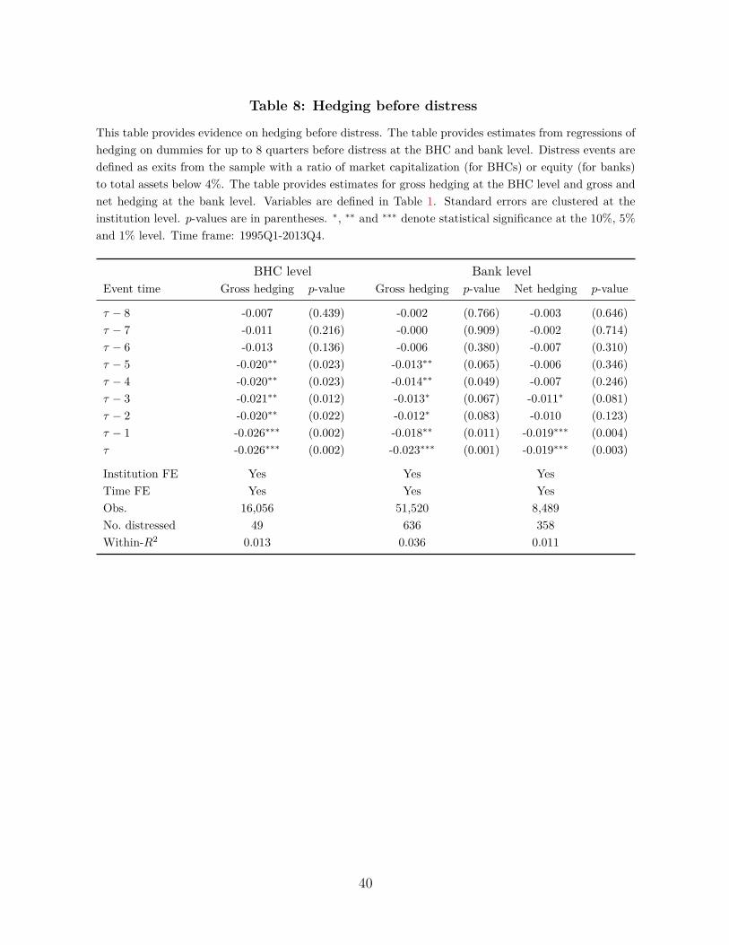
Table 8: Hedging before distress

This table provides evidence on hedging before distress. The table provides estimates from regressions ofhedging on dummies for up to 8 quarters before distress at the BHC and bank level. Distress events aredefined as exits from the sample with a ratio of market capitalization (for BHCs) or equity (for banks)to total assets below 4%. The table provides estimates for gross hedging at the BHC level and gross andnet hedging at the bank level. Variables are defined in Table 1. Standard errors are clustered at theinstitution level. p-values are in parentheses. ∗, ∗∗ and ∗∗∗ denote statistical significance at the 10%, 5%and 1% level. Time frame: 1995Q1-2013Q4.

BHC level Bank levelEvent time Gross hedging p-value Gross hedging p-value Net hedging p-value

τ − 8 -0.007 (0.439) -0.002 (0.766) -0.003 (0.646)τ − 7 -0.011 (0.216) -0.000 (0.909) -0.002 (0.714)τ − 6 -0.013 (0.136) -0.006 (0.380) -0.007 (0.310)τ − 5 -0.020∗∗ (0.023) -0.013∗∗ (0.065) -0.006 (0.346)τ − 4 -0.020∗∗ (0.023) -0.014∗∗ (0.049) -0.007 (0.246)τ − 3 -0.021∗∗ (0.012) -0.013∗ (0.067) -0.011∗ (0.081)τ − 2 -0.020∗∗ (0.022) -0.012∗ (0.083) -0.010 (0.123)τ − 1 -0.026∗∗∗ (0.002) -0.018∗∗ (0.011) -0.019∗∗∗ (0.004)τ -0.026∗∗∗ (0.002) -0.023∗∗∗ (0.001) -0.019∗∗∗ (0.003)

Institution FE Yes Yes YesTime FE Yes Yes YesObs. 16,056 51,520 8,489No. distressed 49 636 358Within-R2 0.013 0.036 0.011

40

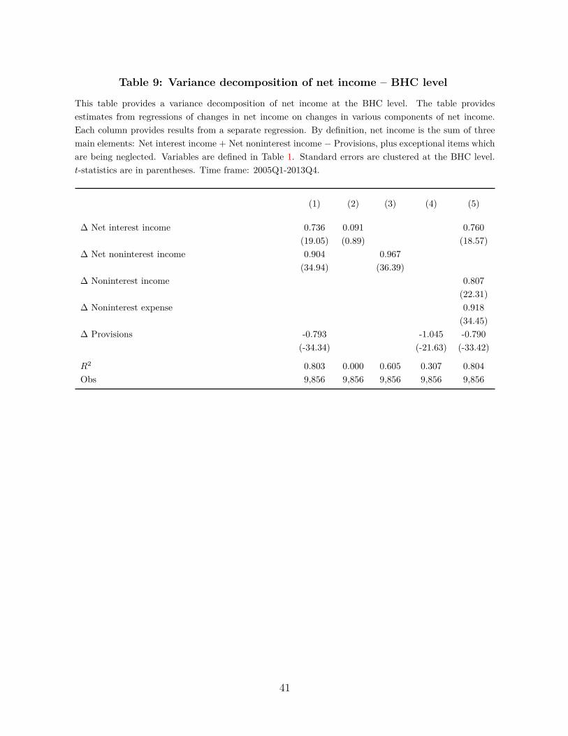
Table 9: Variance decomposition of net income – BHC level

This table provides a variance decomposition of net income at the BHC level. The table providesestimates from regressions of changes in net income on changes in various components of net income.Each column provides results from a separate regression. By definition, net income is the sum of threemain elements: Net interest income + Net noninterest income − Provisions, plus exceptional items whichare being neglected. Variables are defined in Table 1. Standard errors are clustered at the BHC level.t-statistics are in parentheses. Time frame: 2005Q1-2013Q4.

(1) (2) (3) (4) (5)

∆ Net interest income 0.736 0.091 0.760(19.05) (0.89) (18.57)

∆ Net noninterest income 0.904 0.967(34.94) (36.39)

∆ Noninterest income 0.807(22.31)

∆ Noninterest expense 0.918(34.45)

∆ Provisions -0.793 -1.045 -0.790(-34.34) (-21.63) (-33.42)

R2 0.803 0.000 0.605 0.307 0.804Obs 9,856 9,856 9,856 9,856 9,856

41

Table 10: Instrumenting net income with changes in house prices

This table provides evidence on instrumental variable regressions of gross hedging on net income at theBHC and bank level. The sample is restricted to institutions with above-median loans secured by realestate. The table provides both the OLS estimates and the estimates from the first and second stageof instrumental variables regressions. Net income is instrumented by changes in weighted-average houseprices over the past 8 quarters. The instrumental variable regressions include institution fixed effects.Variables are defined in Table 1. Standard errors are clustered at the institution level. p-values are inparentheses. ∗, ∗∗ and ∗∗∗ denote statistical significance at the 10%, 5% and 1% level. Time frame:2005Q1-2013Q4.

BHC level Bank level

OLS IV OLS IV

First stage 0.251∗∗ 0.113∗∗

(0.037) (0.033)Within-R2 0.096 0.053

Net income 0.185∗ 0.254∗∗ 0.049∗ 0.086∗∗

(0.062) (0.049) (0.075) (0.044)Within-R2 0.008 0.003 0.003 0.001

42

Table 11: Effect of net worth on hedging – Difference-in-differences estimates

This table provides the difference-in-differences estimates at the BHC level (Panel A) and the banklevel (Panel B) for three specifications of the treatment. The dependent variable is gross hedging. Thetreatment group is defined as the bottom 30% and the control group at the top 30% of institutions in2009 in terms of net income (Columns (1) to (3)), deposit weighted-average ZIP code level house pricechanges in 2007Q1 through 2008Q4 (Columns (4) to (6)), and deposit weighted-average MSA level Saiz(2010) housing supply elasticity in 2008Q4 (Columns (7) to (9)). We restrict the sample to institutionswith above-median loans secured by real estate to total assets in 2008Q4. In both panels, the sample isrestricted to institutions that hedge at least once before the treatment. Variables are defined in Table 1.Standard errors are clustered at the institution level. p-values are in parentheses. ∗, ∗∗ and ∗∗∗ denotestatistical significance at the 10%, 5% and 1% level. Time frame: 2005Q1-2013Q4.

Treatment Net income House price change Housing supply elasticity(1) (2) (3) (4) (5) (6) (7) (8) (9)

Post-event Year Year Post-event Year Year Post-event Year Yeardummy dummies dummies dummy dummies dummies dummy dummies dummies

Panel A: BHC level

2009 and -0.029∗∗ -0.040∗ -0.042∗

after (0.042) (0.056) (0.051)2009 -0.020 -0.022∗∗ -0.022 -0.026∗ -0.027∗∗ -0.096∗∗

(0.259) (0.025) (0.246) (0.098) (0.026) (0.037)2010 -0.039∗∗ -0.042∗∗∗ -0.022 -0.026 -0.027∗∗ -0.092∗∗

(0.026) (0.009) (0.154) (0.111) (0.035) (0.043)2011 -0.038∗∗ -0.035∗∗ -0.044∗ -0.051∗∗ -0.026∗∗ -0.059∗

(0.037) (0.046) (0.055) (0.049) (0.041) (0.056)2012 -0.019 -0.020∗ -0.042∗ -0.039∗ -0.021∗ -0.055∗

(0.263) (0.089) (0.065) (0.085) (0.054) (0.062)2013 -0.031∗ -0.033∗ -0.025 -0.016 -0.019∗ -0.047

(0.099) (0.053) (0.147) (0.326) (0.096) (0.112)BHC FE No No Yes No No Yes No No YesTime FE Yes Yes Yes Yes Yes Yes Yes Yes Yes

Panel B: Bank level

2009 and -0.015∗∗∗ -0.018∗ -0.005after (0.009) (0.068) (0.345)2009 -0.019∗∗ -0.017∗∗ -0.014∗ -0.018∗ -0.002 -0.003

(0.042) (0.031) (0.094) (0.087) (0.756) (0.621)2010 -0.010 -0.017∗∗ -0.014∗ -0.018∗ -0.002 -0.003

(0.181) (0.019) (0.094) (0.087) (0.756) (0.621)2011 0.001 0.006 -0.022∗ -0.025∗ -0.004 -0.003

(0.910) (0.390) (0.056) (0.064) (0.458) (0.352)2012 -0.021∗∗∗ -0.027∗∗∗ -0.019 -0.021 -0.010 -0.006

(0.008) (0.000) (0.125) (0.100) (0.555) (0.489)2013 −0.028∗∗∗ -0.018∗∗ -0.008 -0.010 0.002 0.014

(0.000) (0.017) (0.341) (0.239) (0.672) (0.534)Bank FE No No Yes No No Yes No No YesTime FE Yes Yes Yes Yes Yes Yes Yes Yes Yes

43

Table 12: Robustness – Pre-treatment differences and effect on maturity gap

This table provides two sets of robustness estimates comparing the treatment and control groups using netincome to define the treatment variable as in columns (1) to (3) in Table 11. Panel A provides estimatesfrom a difference-in-differences specification at the BHC level as in columns (1) to (3) in Panel A ofTable 11 but includes treatment-dummies for the pre-treatment period as well. Panel B provides estimatesfrom a difference-in-differences specification using the maturity gap as the dependent variable using dataat both the BHC and bank level. In both panels, the sample is restricted to institutions that hedge atleast once before the treatment. Variables are defined in Table 1. Standard errors are clustered at theinstitution level. p-values are in parentheses. ∗, ∗∗ and ∗∗∗ denote statistical significance at the 10%, 5%and 1% level. Time frame: 2005Q1-2013Q4.

Panel A: Difference-in-difference estimates with pre-treatment dummies

Year Yeardummies dummies

2005 -0.014 (0.331) -0.003 (0.784)2006 -0.010 (0.499) 0.008 (0.444)2007 -0.007 (0.626) -0.000 (0.989)2008 – –2009 -0.028∗ (0.085) -0.017 (0.134)2010 -0.047∗∗∗ (0.004) -0.029∗∗ (0.010)2011 -0.046∗∗∗ (0.005) -0.028∗∗ (0.015)2012 -0.027∗ (0.095) -0.030∗∗∗ (0.009)2013 -0.039∗∗ (0.019) -0.036∗∗∗ (0.002)

BHC FE No YesTime FE Yes Yes

Panel B: Effect of treatment on maturity gap

BHC level Bank levelPost-event p-value Year p-value Post-event p-value Year p-valuedummy dummies dummy dummies

2009 and after -0.025 (0.352) -0.038 (0.232)2009 -0.087∗∗ (0.021) -0.094∗∗∗ (0.012)2010 -0.019 (0.609) -0.036 (0.303)2011 -0.021 (0.569) -0.041 (0.204)2012 0.008 (0.817) -0.006 (0.862)2013 -0.008 (0.815) -0.014 (0.663)

44

Table 13: Derivatives trading and net worth

This table provides evidence on the relation between trading and net worth. Trading is measured asgross derivatives positions held for trading normalized by total assets. Panel A provides estimates fromregressions of trading on our measures of net worth at the BHC level from three specifications: a BHC-mean Tobit, a Tobit with time fixed effects, and a regression with BHC fixed effects. Panel B providesestimates from regressions of trading on dummies for up to 8 quarters before distress at the BHC andbank level. Variables are defined in Table 1. Standard errors are clustered at the institution level;standard errors for BHC-mean regressions are robust. p-values are in parentheses. ∗, ∗∗ and ∗∗∗ denotestatistical significance at the 10%, 5% and 1% level. Time frame: 1995Q1-2013Q4.

Panel A: OLS and fixed effect regressions

Model Size Mkt. cap. Mkt. cap./ Net Div. Rating Net worthAssets income index

BHC-mean 0.579∗∗∗ 0.484∗∗∗ 0.600 9.361∗ 374.661∗∗∗ 0.872∗∗∗ 0.303∗∗∗

Tobit (0.000) (0.000) (0.509) (0.089) (0.000) (0.000) (0.000)R2 0.267 0.215 0.000 0.001 0.011 0.036 0.036

Tobit 0.590∗∗∗ 0.511∗∗∗ 3.300∗∗∗ 11.459∗∗∗ 164.830∗∗∗ 0.809∗∗∗ 0.358∗∗∗

with time FE (0.000) (0.000) (0.000) (0.000) (0.000) (0.000) (0.000)R2 0.318 0.279 0.014 0.009 0.012 0.045 0.063

BHC FE 0.082∗∗∗ 0.020∗∗∗ 0.692∗∗∗ 1.172∗∗∗ 5.965 0.040 0.096∗∗

(0.000) (0.010) (0.000) (0.001) (0.471) (0.127) (0.024)Within-R2 0.009 0.042 0.049 0.044 0.042 0.096 0.134

Panel B: Derivatives trading before distress

BHC level Bank levelEvent time Gross trading p-value Gross trading p-valueτ − 8 -0.020 (0.458) 0.009 (0.417)τ − 7 -0.045∗∗∗ (0.002) 0.011 (0.396)τ − 6 -0.038∗∗∗ (0.009) 0.012 (0.357)τ − 5 -0.042∗∗∗ (0.009) 0.020 (0.491)τ − 4 -0.041∗∗ (0.014) 0.014 (0.457)τ − 3 -0.053∗∗∗ (0.006) 0.009 (0.544)τ − 2 -0.052∗∗∗ (0.005) 0.012 (0.250)τ − 1 -0.053∗∗ (0.010) 0.013 (0.241)τ -0.059∗∗∗ (0.003) 0.006 (0.599)

Institution FE Yes YesTime FE Yes YesObs. 5,955 18,540No. distressed 10 224Within-R2 0.042 0.005

45

Table 14: Maturity gap and net worth

This table provides evidence on the relation between the maturity gap and net worth. Panel A providesestimates from pooled time series-cross section OLS regressions of the maturity gap on our measures ofnet worth at the BHC level. Panel B provides estimates from regressions of the maturity gap on dummiesfor up to 8 quarters before distress at the BHC and bank level. Distress events are defined as in Table 8.Variables are defined in Table 1. Standard errors are clustered at the institution level. p-value are inparentheses. ∗, ∗∗ and ∗∗∗ denote statistical significance at the 10%, 5% and 1% level. Time frame:1995Q1-2013Q4.

Panel A: Maturity gap and net worth

Size Mkt. cap. Mkt. cap. Net Div. Rating Net worth/ Assets income index

Pooled OLS 0.030∗∗∗ 0.029∗∗∗ 0.681∗∗∗ 1.211∗∗∗ -1.215 0.090∗∗∗ 0.022∗∗∗

(0.000) (0.000) (0.000) (0.001) (0.794) (0.000) (0.000)

Time FE Yes Yes Yes Yes Yes Yes YesBHC cluster Yes Yes Yes Yes Yes Yes YesR2 0.093 0.104 0.077 0.043 0.049 0.187 0.058

Panel B: Maturity gap before distress

BHC level Bank levelEvent time Maturity gap p-value Maturity gap p-valueτ − 8 0.001 (0.909) 0.012 (0.714)τ − 7 -0.023 (0.241) 0.005 (0.887)τ − 6 -0.019 (0.363) -0.028 (0.428)τ − 5 -0.024 (0.227) -0.043 (0.231)τ − 4 -0.036∗ (0.090) -0.046 (0.216)τ − 3 -0.048∗∗ (0.040) -0.056 (0.140)τ − 2 -0.051∗∗ (0.030) -0.071∗ (0.060)τ − 1 -0.073∗∗∗ (0.003) -0.087∗∗ (0.029)τ -0.111∗∗∗ (0.000) -0.120∗∗∗ (0.004)

Institution FE Yes YesTime FE Yes YesObs. 22,699 48,453No. distressed 49 636Within-R2 0.052 0.132

46

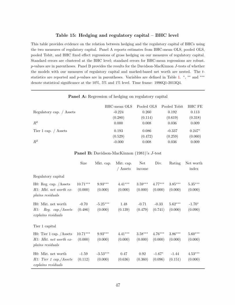
Table 15: Hedging and regulatory capital – BHC level

This table provides evidence on the relation between hedging and the regulatory capital of BHCs usingthe two measures of regulatory capital. Panel A reports estimates from BHC-mean OLS, pooled OLS,pooled Tobit, and BHC fixed effect regressions of gross hedging on our measures of regulatory capital.Standard errors are clustered at the BHC level; standard errors for BHC-mean regressions are robust.p-values are in parentheses. Panel B provides the results for the Davidson-MacKinnon J-tests of whetherthe models with our measures of regulatory capital and marked-based net worth are nested. The t-statistics are reported and p-values are in parentheses. Variables are defined in Table 1. ∗, ∗∗ and ∗∗∗

denote statistical significance at the 10%, 5% and 1% level. Time frame: 1996Q1-2013Q4.

Panel A: Regression of hedging on regulatory capital

BHC-mean OLS Pooled OLS Pooled Tobit BHC FERegulatory cap. / Assets -0.224 0.260 0.192 0.113

(0.280) (0.114) (0.619) (0.318)R2 0.000 0.008 0.036 0.009

Tier 1 cap. / Assets 0.193 0.086 -0.337 0.247∗

(0.529) (0.472) (0.259) (0.060)R2 -0.000 0.008 0.036 0.009

Panel B: Davidson-MacKinnon (1981)’s J-test

Size Mkt. cap. Mkt. cap. Net Div. Rating Net worth/ Assets income index

Regulatory capital

H0: Reg. cap. /Assets 10.71∗∗∗ 9.93∗∗∗ 4.41∗∗∗ 3.59∗∗∗ 4.77∗∗∗ 3.85∗∗∗ 5.35∗∗∗

H1: Mkt. net worth ex-plains residuals

(0.000) (0.000) (0.000) (0.000) (0.000) (0.000) (0.000)

H0: Mkt. net worth -0.70 -5.25∗∗∗ 1.48 -0.71 -0.33 5.62∗∗∗ -1.70∗

H1: Reg. cap./Assetsexplains residuals

(0.486) (0.000) (0.139) (0.479) (0.741) (0.000) (0.090)

Tier 1 capital

H0: Tier 1 cap. /Assets 10.71∗∗∗ 9.93∗∗∗ 4.41∗∗∗ 3.58∗∗∗ 4.76∗∗∗ 3.86∗∗∗ 5.60∗∗∗

H1: Mkt. net worth ex-plains residuals

(0.000) (0.000) (0.000) (0.000) (0.000) (0.000) (0.000)

H0: Mkt. net worth -1.59 -3.53∗∗∗ 0.47 0.92 -1.67∗ -1.44 4.53∗∗∗

H1: Tier 1 cap./Assetsexplains residuals

(0.112) (0.000) (0.636) (0.360) (0.096) (0.151) (0.000)

47

Figure 1: Distribution of measures of BHC net worth

This figure plots the distribution of our measures of net worth. There is one cross-sectional box plotfor each quarter from 1995Q1 to 2013Q4. In each of them, the horizontal dash is the median and thediamond is the mean. The whiskers represent the 5th and 95th percentiles. The grey rectangle representsthe 25th and 75th percentiles. Variables are defined in Table 1.

48

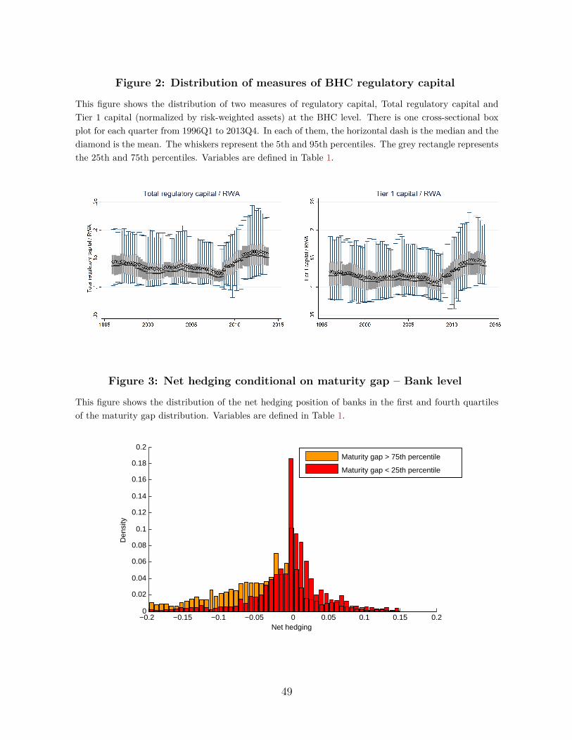
Figure 2: Distribution of measures of BHC regulatory capital

This figure shows the distribution of two measures of regulatory capital, Total regulatory capital andTier 1 capital (normalized by risk-weighted assets) at the BHC level. There is one cross-sectional boxplot for each quarter from 1996Q1 to 2013Q4. In each of them, the horizontal dash is the median and thediamond is the mean. The whiskers represent the 5th and 95th percentiles. The grey rectangle representsthe 25th and 75th percentiles. Variables are defined in Table 1.

Figure 3: Net hedging conditional on maturity gap – Bank level

This figure shows the distribution of the net hedging position of banks in the first and fourth quartilesof the maturity gap distribution. Variables are defined in Table 1.

−0.2 −0.15 −0.1 −0.05 0 0.05 0.1 0.15 0.20

0.02

0.04

0.06

0.08

0.1

0.12

0.14

0.16

0.18

0.2

Den

sity

Net hedging

Maturity gap > 75th percentile

Maturity gap < 25th percentile

49

Figure 4: Hedging before distress events

This figure shows the extent of interest rate hedging in the eight quarters preceding distress. Panel Ashows the mean and median gross hedging at the BHC level. Panel B shows gross hedging (left panel)and net hedging (right panel), respectively, at the bank level. Hedging measures are normalized by totalassets. The sample is restricted to institutions that hedge at least once between τ − 8 and τ . In bothpanels, the sample is restricted to institutions that are present in all quarters between τ − 8 and τ .Distress events are defined as in Table 8. Variables are defined in Table 1.

Panel A: Gross hedging before distress – BHC level

0

0.01

0.02

0.03

0.04

0.05

0.06

τ−8 τ−7 τ−6 τ−5 τ−4 τ−3 τ−2 τ−1 τ Quarters before distress

Gro

ss h

edgi

ng /

Tot

al a

sset

s −

BH

C le

vel

MeanMedian

Panel B: Gross hedging and net hedging before distress – bank level

0

0.01

0.02

0.03

0.04

0.05

0.06

τ−8 τ−7 τ−6 τ−5 τ−4 τ−3 τ−2 τ−1 τ Quarters before distress

Gro

ss h

edgi

ng /

Tot

al a

sset

s −

Ban

k le

vel

MeanMedian

0

0.01

0.02

0.03

0.04

0.05

0.06

τ−8 τ−7 τ−6 τ−5 τ−4 τ−3 τ−2 τ−1 τ Quarters before distress

Net

hed

ging

/ T

otal

ass

ets

− B

ank

leve

l

MeanMedian

50

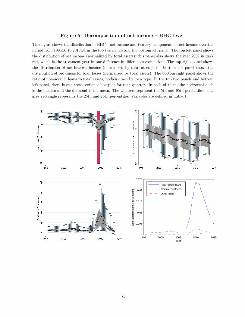
Figure 5: Decomposition of net income – BHC level

This figure shows the distribution of BHCs’ net income and two key components of net income over theperiod from 1995Q1 to 2013Q4 in the top two panels and the bottom left panel. The top left panel showsthe distribution of net income (normalized by total assets); this panel also shows the year 2009 in darkred, which is the treatment year in our difference-in-differences estimation. The top right panel showsthe distribution of net interest income (normalized by total assets); the bottom left panel shows thedistribution of provisions for loan losses (normalized by total assets). The bottom right panel shows theratio of non-accrual loans to total assets, broken down by loan type. In the top two panels and bottomleft panel, there is one cross-sectional box plot for each quarter. In each of them, the horizontal dashis the median and the diamond is the mean. The whiskers represent the 5th and 95th percentiles. Thegrey rectangle represents the 25th and 75th percentiles. Variables are defined in Table 1.

1995 2000 2005 2010 20150

0.005

0.01

0.015

0.02

0.025

Year

Non

−ac

crua

l loa

ns /

Tot

al a

sset

s

Real−estate loans

Commercial loans

Other loans

51

Figure 6: Effect of drop in net worth – Difference-in-differences – BHC level

This figure shows (gross) derivatives hedging (net of BHC fixed effects), normalized by total assets,for BHCs in the treatment and control group from 2005Q1 to 2013Q4. The sample is restricted toinstitutions that hedge at least once before the treatment year. Variables are defined in Table 1.

2005 2006 2007 2008 2009 2010 2011 2012 2013 2014−0.03

−0.02

−0.01

0

0.01

0.02

0.03

Year

Gro

ss h

edgi

ng (

net o

f BH

C F

E)

Treated

Control

Figure 7: Maturity gap in treatment and control group – BHC level

This figure shows the maturity gap (net of BHC fixed effects) for BHCs in the treatment and controlgroup from 2005Q1 to 2013Q4. The sample is restricted to institutions that hedge at least once beforethe treatment year. Variables are defined in Table 1.

2005 2006 2007 2008 2009 2010 2011 2012 2013 2014−0.1

−0.05

0

0.05

0.1

Year

Mat

urity

gap

(ne

t of B

HC

FE

)

Treated

Control

52

Figure 8: Trading and maturity gap before distress events

This figure shows trading by banks and the maturity gap of BHCs and banks in the eight quarterspreceding distress. Panel A shows gross interest rate derivatives trading (normalized by total assets)at the bank level. The sample is restricted to banks that trade at least once between τ − 8 and τ .Panel B shows the maturity gap at the BHC and bank level. In both panels, the sample is restrictedto institutions that are present in all quarters between τ − 8 and τ . Distress events are defined as inTable 8. Variables are defined in Table 1.

Panel A: Trading before distress – bank level

0

0.2

0.4

0.6

0.8

1

τ−8 τ−7 τ−6 τ−5 τ−4 τ−3 τ−2 τ−1 τ Quarters before distress

Tra

ding

/ T

otal

ass

ets

− B

ank

leve

l

MeanMedian (× 10)

Panel B: Maturity gap before distress – BHC and bank level

−0.2

−0.15

−0.1

−0.05

0

0.05

0.1

0.15

τ−8 τ−7 τ−6 τ−5 τ−4 τ−3 τ−2 τ−1 τ Quarters before distress

Mat

urity

gap

− B

HC

leve

l

MeanMedian

−0.12

−0.1

−0.08

−0.06

−0.04

−0.02

0

0.02

0.04

τ−8 τ−7 τ−6 τ−5 τ−4 τ−3 τ−2 τ−1 τ Quarters before distress

Mat

urity

gap

− B

ank

leve

l

MeanMedian

53