Embed Size (px)
Citation preview
Risk Perceptions of Arsenic in Tap Water and Consumption of Bottled
Water
Paul M. Jakus Utah State University
Dept. of Applied Economics UMC 3530
Logan, UT 84322-3530 [email protected]
W. Douglass Shaw Texas A&M University
To N. Nguyen
University of Tennessee
Mark Walker University of Nevada, Reno
Selected Paper prepared for presentation at the Agricultural and Applied Economics Association 2009 AAEA & ACCI Joint Annual Meeting, Milwaukee,
Wisconsin, July 26-29, 2009 Copyright 2009 by Paul M. Jakus, W. Douglass Shaw, To N. Nguyen, and Mark Walker, All rights reserved. Readers may make verbatim copies of this document for non-commercial purposes by any means, provided that this copyright notice appears on all such copies.
1
Risk Perceptions of Arsenic in Tap Water and Consumption of Bottled Water
Abstract: The demand for bottled water has increased rapidly over the past decade, but
bottled water is extremely costly compared to tap water. The convenience of bottled
water surely matters to consumers, but are others factors at work? This manuscript
examines whether purchases of bottled water are associated with the perceived risk of tap
water. All of the past studies on bottled water consumption have used simple scale
measures of perceived risk that do not correspond to risk measures used by risk analysts.
We elicit a probability-based measure of risk and find that as perceived risks rise,
expenditures for bottled water rise.
Risk Perceptions of Arsenic in Tap Water and Consumption of Bottled Water 1
2
3
4
5
6
7
8
9
10
11
12
13
14
15
16
17
18
19
20
21
22
Introduction
Global bottled water consumption was about 41 billion gallons in 2005, a 57
percent increase over consumption in 1999 (Arnold and Larson, 2006). In the United
States today bottled water constitutes a significant proportion of the beverage industry’s
sales, with nearly 10% growth in per capita consumption between 1999 and 2005 and the
share of bottled water in the beverage market moving ahead of coffee. Sellers include
members of the soda industry; for example, the Coca-Cola Company sells the Dasani
brand of bottled water whereas Pepsicola sells the Aquafina brand. In the late 1990’s
about 54% of the U.S. population regularly consumed bottled water (Olson, 1999), and
the number may be as high as 70% today. Generally speaking, tap water is safe to drink
in most areas of the U.S., so one could question why people in the U.S. drink bottled
water, especially when bottled water can be 240 and 10,000 times more expensive than
tap water (Ferrier, 2001).1 Is it rational to purchase something that can be up to 10,000
times more expensive than a near perfect substitute? While bottled water may be very
convenient for consumers, surely there must be other factors at work in the burgeoning
demand for bottled water.
In this manuscript we focus on the role that perceived risks of tap water play in
the demand for bottled water. Our study centers on a population that is known to be at
risk from arsenic contamination of publicly supplied water or of private well water. We
begin by reviewing the drinking water literature and find that none of these studies uses a
measure of perceived risk corresponding to known exposures. We then describe our data,
1 Indeed, if one considers water obtained at, say, the workplace drinking fountain as a free good, then bottled water is infinitely more expensive than tap water.
1
1
2
3
4
5
6
7
8
9
10
11
12
13
14
15
16
17
18
19
20
21
22
23
which were collected in communities in which respondents are exposed to arsenic
concentrations in excess of current drinking water standards. In particular, we elicit
perceived risk of arsenic exposure in a way that can be evaluated against scientists’ best
available measures of mortality risk. Models linking the probability-based perceived risk
to community arsenic concentrations are presented, after which we examine how
expenditures for bottled water vary according to perceived risk. Perceived risk is found
to be a statistically significant factor in determining bottled water expenditures.
Motivation/Literature Review
Given the high cost of bottled water relative to tap water, one might reasonably
ask why people buy bottled water. From a purely price perspective, are people who
consume bottled water simply irrational? Cherry, Crocker and Shogren [2003] define
rational behavior as people making the best decisions they can with the resources
available to them. Rationality, they argue, may be a scarce commodity because of
constraints on individuals’ cognitive and computational skills. Are people unable to
compute the cost of bottled water such that they do not realize just how expensive it
really is relative to tap water? If people do understand the relative prices, then we might
suspect purchases of bottled water are irrational unless we can find a strong off-setting
reason for its purchase.
In addition to price, there are other factors that distinguish bottled water from tap
water. Bottles of one liter or less are very convenient for those traveling or at work.
Larger containers used for in-home consumption may allow the consumer to purchase
water of better quality than tap water: it may taste better, smell better, look better, or pose
less of a health risk. It is this last characteristic that is of concern in this paper. Data we
2
1
2
3
4
5
6
7
8
9
10
11
12
13
14
15
16
17
18
19
20
21
22
23
have collected allows us to investigate whether people purchase bottled water for the very
rational reason of avoiding risk.
Averting Behavior Models
Averting behavior models explicitly or implicitly assume that households “produce”
better health by using inputs to reduce the adverse consequences of exposure to toxic or
harmful substances: people will engage in activities or purchases designed to protect
themselves from health risks. The subject of water quality has appeared frequently in the
averting behavior literature but many of these studies do not directly address the issue of
perceived risks of exposure to contaminated water. For example, Smith and Desvousges
[1986] found that 30% of households in their Boston, Massachusetts sample said they
purchased bottled water expressly to avoid hazardous wastes, but the authors were unable
to link this behavior directly to risk perceptions. Larson and Gnedenko [1999] estimate
several models of whether individuals engage in different types of averting behavior.
The authors report that people are more likely to purchase bottled water when their
incomes are higher but the study did not include a measure of risk. Yoo [2003] focuses
on a statistical model relating bottle water purchases to demographics, concluding that
more affluent households with young children are more likely to purchase bottled water if
they have reason to suspect their water quality; Yoo and Yang [2000], using the same
data set, find similar results with a slightly different model. The data set used in both
analyses by Yoo does not appear to contain information on perceived risks faced by the
households, though it contains some information regarding perceived water quality.
Similarly, Rosado et al. [2006] and McConnell and Rosado [2004] examine averting
choices as a function of the costs of each activity and demographic factors but, once
3
again, do not include an objective or subjective measure of risk. Um et al. [2002] find
that perceived quality of drinking water affects averting behavior, but the models make
no link to perceived health risks of consuming tap water.
1
2
3
4
5
6
7
8
9
10
11
12
13
14
15
16
17
18
19
20
21
22
23
We have found few studies linking the perceived risk of drinking water to
associated averting behaviors, and none of those have used a measure of risk comparable
to the probability-based measure used by risk analysts. Instead, economists have
generally captured the influence of risk concerns through the use of a qualitative scale or
a dummy variable rather than a technical measure of risk. Abdalla et al. [1992] use a 5-
point scale of perceived health risk for exposure to trichloroethylene contamination in
groundwater and find that expenditures on averting activities increase as perceived risk
increases. Abrahams et al. [2000] use a very simple measure of risk: a binary variable
takes the value of zero if people think their tap water is safe and the value of one if they
think it is somewhat unsafe or unsafe. The authors conclude that perceived risk is more
important in determining averting actions than other water quality factors. Janmaat
[2007] used principal component analysis to develop a measure of perceived risk
concerns from a variety of qualitative responses to survey questions, a fundamentally
different approach from that used by previous authors but one that still does not permit
the analyst to compare perceived risk to objectively measured risk. This risk measure,
however, was not a statistically significant determinant of household water treatment
activities.
Objective and Perceived Risk
The scale-based risk measures used in the studies cited above have two key flaws. First,
different people will use the scale-based measures differently: one person’s “three” on a
4
1
2
3
4
5
6
7
8
9
10
11
12
13
14
15
16
17
18
19
20
21
22
23
five-point qualitative scale may or may not mean the same thing as another person’s
“three”. That is, the same point on a rating scale may measure perceived risks that
actually differ across the two individuals (see the discussion of various risk ratings in
Viscusi and Hakes, 2003). A second problem is that scale measures such as those used in
previous studies, and the principal components measures used by Janmaat [2007], can
establish only an ordinal link between contaminant exposures and perceived risks. The
analyst may be able to estimate a statistical relationship between the perceived risk scale
and exposure, but the model will not yield information on how the qualitative scale
corresponds to scientists’ best estimates of probability-based risk.
Risk analysts estimate health risks using population-level probabilities of a given
health outcome, calibrated by exposures. For example, it is estimated that the
“background” level of lung and bladder cancer is about 60 deaths per 100,000 people, but
exposure to arsenic in drinking water at a concentration of 50 parts per billion for twenty
years will increase the mortality rate to 1000 cases per 100,000 people, or 1 in one
hundred (see U.S. EPA, 2000). If a person smokes and is exposed to arsenic at 50 ppb
for twenty years, the rate rises to 2000 deaths per 100,000. These risks are often
converted to probabilities (0.0006, 0.01, and 0.02, respectively). If perceived risk can be
elicited in the form of probabilities rather than a qualitative scale, then one may use
statistical models to evaluate the degree to which subjectively evaluated risk corresponds
to the objective risk as measured by scientists.
This is important because perceived risks are often quite different from science-
based estimates of risk (Slovic, 1987, provides the seminal reference). Slovic found that
dangers to which people choose to voluntarily expose themselves, such as alcohol
5
1
2
3
4
5
6
7
8
9
10
11
12
13
14
15
16
17
18
19
20
21
22
23
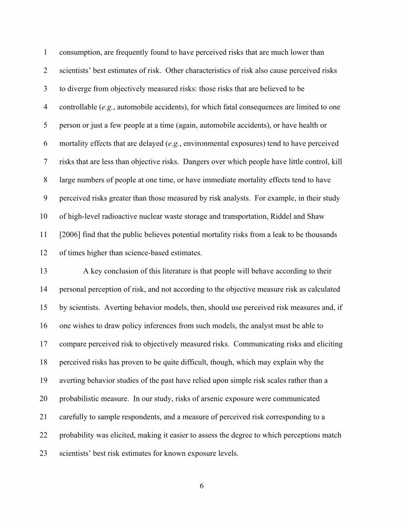
consumption, are frequently found to have perceived risks that are much lower than
scientists’ best estimates of risk. Other characteristics of risk also cause perceived risks
to diverge from objectively measured risks: those risks that are believed to be
controllable (e.g., automobile accidents), for which fatal consequences are limited to one
person or just a few people at a time (again, automobile accidents), or have health or
mortality effects that are delayed (e.g., environmental exposures) tend to have perceived
risks that are less than objective risks. Dangers over which people have little control, kill
large numbers of people at one time, or have immediate mortality effects tend to have
perceived risks greater than those measured by risk analysts. For example, in their study
of high-level radioactive nuclear waste storage and transportation, Riddel and Shaw
[2006] find that the public believes potential mortality risks from a leak to be thousands
of times higher than science-based estimates.
A key conclusion of this literature is that people will behave according to their
personal perception of risk, and not according to the objective measure risk as calculated
by scientists. Averting behavior models, then, should use perceived risk measures and, if
one wishes to draw policy inferences from such models, the analyst must be able to
compare perceived risk to objectively measured risks. Communicating risks and eliciting
perceived risks has proven to be quite difficult, though, which may explain why the
averting behavior studies of the past have relied upon simple risk scales rather than a
probabilistic measure. In our study, risks of arsenic exposure were communicated
carefully to sample respondents, and a measure of perceived risk corresponding to a
probability was elicited, making it easier to assess the degree to which perceptions match
scientists’ best risk estimates for known exposure levels.
6
The Sample and Data 1
2
3
4
5
6
7
8
9
10
11
12
13
14
15
16
17
18
19
20
21
22
23
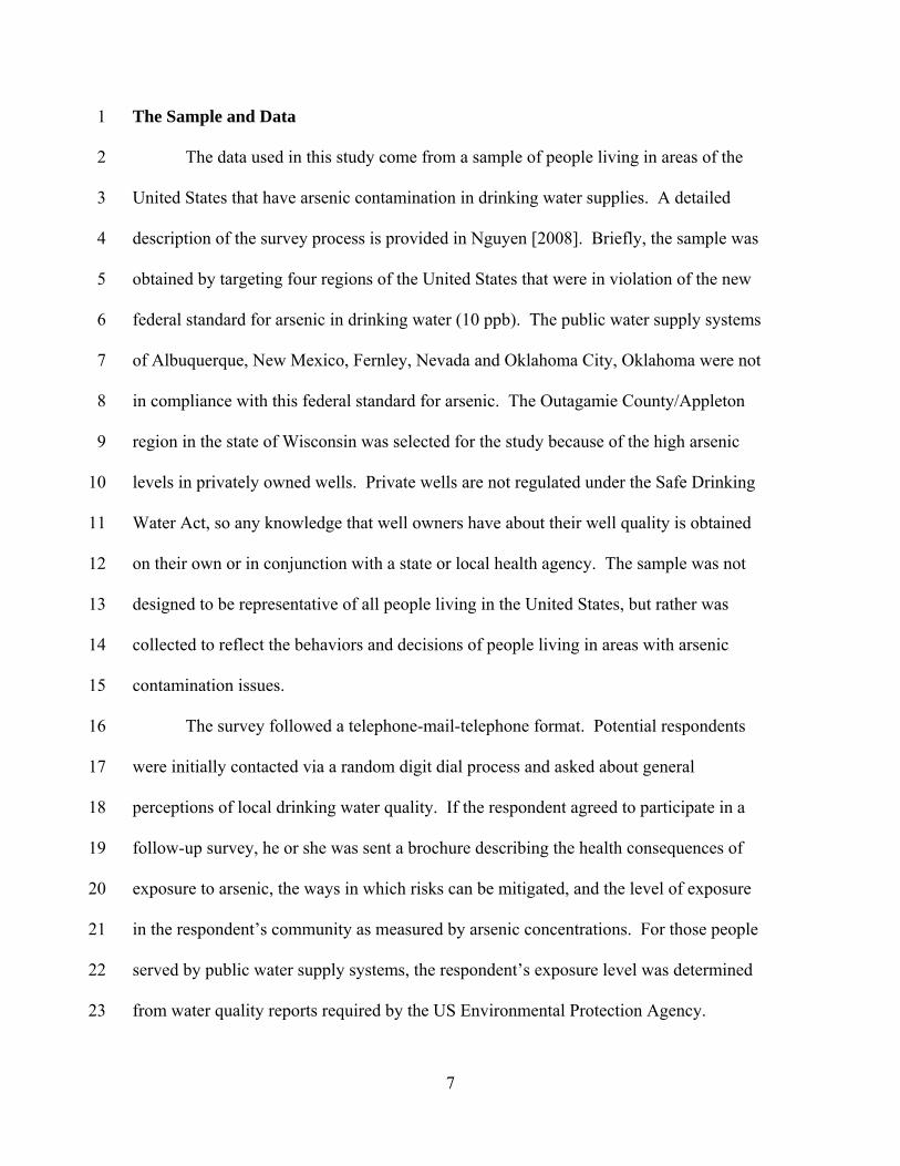
The data used in this study come from a sample of people living in areas of the
United States that have arsenic contamination in drinking water supplies. A detailed
description of the survey process is provided in Nguyen [2008]. Briefly, the sample was
obtained by targeting four regions of the United States that were in violation of the new
federal standard for arsenic in drinking water (10 ppb). The public water supply systems
of Albuquerque, New Mexico, Fernley, Nevada and Oklahoma City, Oklahoma were not
in compliance with this federal standard for arsenic. The Outagamie County/Appleton
region in the state of Wisconsin was selected for the study because of the high arsenic
levels in privately owned wells. Private wells are not regulated under the Safe Drinking
Water Act, so any knowledge that well owners have about their well quality is obtained
on their own or in conjunction with a state or local health agency. The sample was not
designed to be representative of all people living in the United States, but rather was
collected to reflect the behaviors and decisions of people living in areas with arsenic
contamination issues.
The survey followed a telephone-mail-telephone format. Potential respondents
were initially contacted via a random digit dial process and asked about general
perceptions of local drinking water quality. If the respondent agreed to participate in a
follow-up survey, he or she was sent a brochure describing the health consequences of
exposure to arsenic, the ways in which risks can be mitigated, and the level of exposure
in the respondent’s community as measured by arsenic concentrations. For those people
served by public water supply systems, the respondent’s exposure level was determined
from water quality reports required by the US Environmental Protection Agency.
7
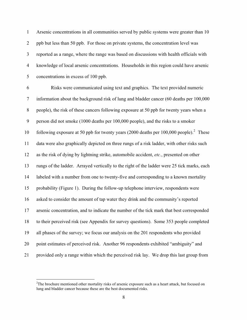
Arsenic concentrations in all communities served by public systems were greater than 10
ppb but less than 50 ppb. For those on private systems, the concentration level was
reported as a range, where the range was based on discussions with health officials with
knowledge of local arsenic concentrations. Households in this region could have arsenic
concentrations in excess of 100 ppb.
1
2
3
4
5
6
7
8
9
10
11
12
13
14
15
16
17
18
19
20
21
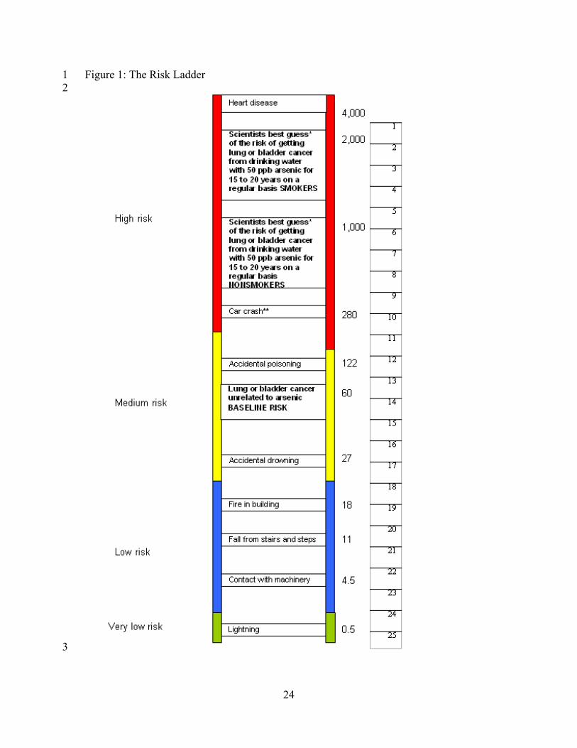
Risks were communicated using text and graphics. The text provided numeric
information about the background risk of lung and bladder cancer (60 deaths per 100,000
people), the risk of these cancers following exposure at 50 ppb for twenty years when a
person did not smoke (1000 deaths per 100,000 people), and the risks to a smoker
following exposure at 50 ppb for twenty years (2000 deaths per 100,000 people).2 These
data were also graphically depicted on three rungs of a risk ladder, with other risks such
as the risk of dying by lightning strike, automobile accident, etc., presented on other
rungs of the ladder. Arrayed vertically to the right of the ladder were 25 tick marks, each
labeled with a number from one to twenty-five and corresponding to a known mortality
probability (Figure 1). During the follow-up telephone interview, respondents were
asked to consider the amount of tap water they drink and the community’s reported
arsenic concentration, and to indicate the number of the tick mark that best corresponded
to their perceived risk (see Appendix for survey questions). Some 353 people completed
all phases of the survey; we focus our analysis on the 201 respondents who provided
point estimates of perceived risk. Another 96 respondents exhibited “ambiguity” and
provided only a range within which the perceived risk lay. We drop this last group from
2The brochure mentioned other mortality risks of arsenic exposure such as a heart attack, but focused on lung and bladder cancer because these are the best documented risks.
8
the analysis because its inclusion greatly increases the statistical complexity of the
analysis (see Nguyen et al., 2008) and distracts from the primary thesis of this study.
1
2
3
4
5
6
7
8
9
10
11
12
13
14
15
16
17
18
19
20
3
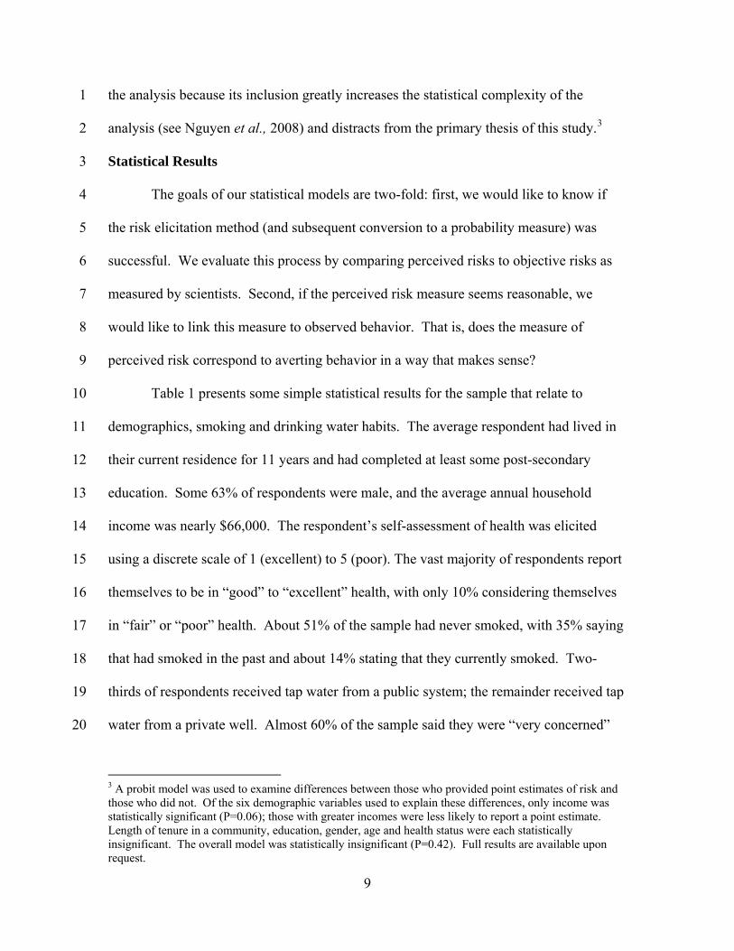
Statistical Results
The goals of our statistical models are two-fold: first, we would like to know if
the risk elicitation method (and subsequent conversion to a probability measure) was
successful. We evaluate this process by comparing perceived risks to objective risks as
measured by scientists. Second, if the perceived risk measure seems reasonable, we
would like to link this measure to observed behavior. That is, does the measure of
perceived risk correspond to averting behavior in a way that makes sense?
Table 1 presents some simple statistical results for the sample that relate to
demographics, smoking and drinking water habits. The average respondent had lived in
their current residence for 11 years and had completed at least some post-secondary
education. Some 63% of respondents were male, and the average annual household
income was nearly $66,000. The respondent’s self-assessment of health was elicited
using a discrete scale of 1 (excellent) to 5 (poor). The vast majority of respondents report
themselves to be in “good” to “excellent” health, with only 10% considering themselves
in “fair” or “poor” health. About 51% of the sample had never smoked, with 35% saying
that had smoked in the past and about 14% stating that they currently smoked. Two-
thirds of respondents received tap water from a public system; the remainder received tap
water from a private well. Almost 60% of the sample said they were “very concerned”
3 A probit model was used to examine differences between those who provided point estimates of risk and those who did not. Of the six demographic variables used to explain these differences, only income was statistically significant (P=0.06); those with greater incomes were less likely to report a point estimate. Length of tenure in a community, education, gender, age and health status were each statistically insignificant. The overall model was statistically insignificant (P=0.42). Full results are available upon request.
9
1
2
3
4
5
6
7
8
9
10
11
12
13
14
15
16
17
18
19
20
21
22
about the water quality in drinking water sources. Water quality concerns were elicited
before mailing the arsenic information brochure and thus represent “prior” perceptions of
water quality. A little over one-third of respondents reported buying bottled water,
though very few of these people relied exclusively upon bottled water for cooking and
drinking. The mean monthly expenditure for bottled water amongst those purchasing
bottled water was $27.
Perceived Risks
Our simple evaluation of the risk elicitation method is presented in Table 2.
Overall, the mean perceived risk of mortality from arsenic contamination at local
concentration levels is 0.0059, or 590 deaths out of 100,000 over twenty years of
exposure at local arsenic concentrations. This is above the background level mortality
risk for lung and bladder cancer in the absence of arsenic contamination (0.0006) but
below that for exposure at 50 ppb (0.01). After controlling for smoking history, the
results are encouraging. Respondents who have never smoked have the lowest perceived
mortality risk (0.0038) whereas those currently smoking have the highest perceived risk
(0.0139). Those who currently smoke, or have had a history of smoking, appear to
understand that smokers are at higher risks from drinking arsenic-laden water.
The results presented in Table 2 do not account for other factors that influence
perceived risk. In particular we are interested in how smoking, the level of arsenic
exposure, and other factors may influence peoples’ perceived risk. We use multivariate
regression analysis to accomplish this, using the regression model
y = β’X + ε
10
where y is perceived risk, X is a set of explanatory variables, β is a set of parameters to be
estimated, and ε is the error term. The elements of X include not only exposure to arsenic
and smoking history, but also other factors suggested by the literature and our focus
group work: the source of drinking water (a public water system or a private well), length
of tenure in the community, and the respondent’s age, gender, educational level, and self-
reported health status.
1
2
3
4
5
6
7
8
9
10
11
12
13
14
15
16
17
18
19
20
21
22
4
Table 3 reports results of our ordinary least squares model of perceived risk. The
longer a respondent had lived in their current residence (Years in Current Residence), the
lower they believe subjective risks are, and this variable is strongly significant. Those
getting tap water from a Public Water System believe themselves to be at higher risk than
those on private systems. Gender and Education appear to have no statistical influence
on perceived arsenic mortality risk. People in poorer health (Health Status) report higher
subjective arsenic risks, perhaps resulting from a belief that they are more vulnerable to
environmental contaminants than those who are in better health.
Consistent with the results presented in Table 2, those who identified themselves
as a Current or Former Smoker have significantly greater perceived risk than those who
have never smoked. All else equal, smokers and former smokers believe that a history of
smoking causes the risks of lung and bladder cancer mortality to rise by an additional 370
deaths per 100,000 people. Our statistical model also shows that perceived mortality
risks rise with exposure to arsenic (PPB). The sign on arsenic concentration is positive
and significant. All else equal, the model indicates that respondents believe mortality
risks rise by 20 deaths per 100,000 people for every one part per billion increase in
4 We are unable to control for other factors that might influence perceived risk, e.g., a history of cancer in the family, the total volume of water consumed, and the amount of water consumed away from home.
11
arsenic concentration. Our finding that perceived risk increases as contaminant exposure
increases is consistent with the analyses of Poe et al. [1998] and Poe and Bishop [1999].
1
2
3
4
5
6
7
8
9
10
11
12
13
14
15
16
17
18
19
20
21
To make a comparison of arsenic mortality risks as assessed by our sample with
scientists’ best estimates of risk, we predict perceived risks under the assumption that
everyone in the sample is exposed to an arsenic concentration of 50 ppb.5 At an exposure
concentration of 50 ppb, but holding all other variables at the levels reported by the
respondent, the mean overall risk for the sample is 0.0069, or 690 cases per 100,000. For
non-smokers the predicted risk was 0.0045, or 450 deaths per 100,000 people, which is
below the best scientific estimate for 50 ppb exposures of 1000 deaths. For those who
had ever smoked the predicted risk was 0.0092, or 920 cases out of 100,000 people; again
this is below the scientists’ best estimate of 2000 deaths per 100,000 people. Our sample
respondents appear to systematically underestimate the risks of arsenic exposure but this
is not unusual. The risk perception literature indicates that lay persons frequently
underestimate the risks that can be controlled, are not catastrophic, and have delayed
health effects (Slovic, 1987; Brewer et al., 2004; Flynn et al., 1993; Rowe and Wright,
2001).
Bottled Water Expenditures
Having established that respondents’ perceived risks are correlated with arsenic exposure
and exacerbating habits (smoking), our next task is to assess whether our measure of
perceived risk affects consumer behavior. Past research has indicated that perceived
water quality and perceived risk, as measured by a qualitative response scale, do affect
5 We estimate of perceived risk by using the model coefficients reported in Table 3 by setting arsenic exposure (PPB) equal to 50 and using the actual values reported by the respondent for all other right hand side variables. Although ordinary least squares was used, we predicted no cases of a negative perceived risk.
12
1
2
3
4
5
6
7
8
9
10
11
12
13
14
15
16
17
18
19
20
21
22
23
the demand for bottled water. Our data do not contain self-reported information on the
actual volume of water used by the household because our focus group work indicated
that households would have a difficult time recalling volumes of water used or purchased.
A somewhat easier question for respondents to answer is their typical monthly
expenditure on bottled water (reported in Table 1). The mean expenditures for those
purchasing bottled water was $27 per month, but some 64% of the sample did not buy
bottled water.
We are interested in expenditures on bottled water, which may be expressed with
the following model,
w = τ’F + υ [1]
where w is the measure of bottled water expenditures, F is a vector of variables
explaining expenditures, τ is a parameter vector to be estimated and υ is the stochastic
error term associated with the model. Under the standard assumptions of an ordinary
least squares (OLS) model, the expected value of the left hand side would be τ’F, but this
approach would not account for all the people who spent no money on bottled water.
That is, the OLS model given above actually measures expected expenditures given that
expenditures were greater than zero.
To gauge the full effects of perceived risk on demand for bottled water, the
modeling procedure must recognize that the majority of people choose not to purchase
bottled. That is, our modeling should reflect a participation decision, or “selection
effect”, that accounts for differences across people in deciding to buy any bottled water at
all, as well as a quantity decision—how much bottled water to buy. Heckman [1979]
formalized the econometric approach to modeling such processes, and variations of this
13
1
2
3
4
5
6
7
8
9
10
11
12
13
14
15
16
17
18
19
20
21
22
23
methodology have become common in the literature (see, for example, Hoehn, 2006; Yoo
and Yang, 2000; or Bockstael et al., 1990).
The model can be thought of as a two-stage decision process, with participation at
the first stage and expenditures at the second. At the first stage the consumer decides if
he or she will consume bottled water,
z* = α’W + u [2]
where z* represents an unobservable index of propensity to purchase bottled water, W is
the vector of variables affecting this propensity, α is a parameter vector to be estimated
and u is the error term. The error terms for equations [1] and [2] are correlated with one
another, causing inconsistency of the OLS estimates in equation [1] had all observations–
purchasers and non-purchasers–been included in the estimation.
z* may be unobservable, yet we can take advantage of an indicator variable, z, to
be used as the basis of a probit specification:
z = 1 if z* > 0
z = 0 if z* ≤ 0
A probit model of participation (z = 1 means the person buys bottled water) will yield
estimates of α, which are used to form the inverse Mill’s ratio, λ = φ(α’W)/Φ(α’W), where
φ(.) and Φ(.) are the standard normal density and cumulative distribution functions,
respectively. The inverse Mill’s ratio is then used as an explanatory variable on the right
hand side of equation [1], so that
w = τ’F + ρσλ
ρ and σ correspond to the correlation of the error terms across equations [1] and [2] and
the standard deviation of the error term in equation [1], respectively. Estimating
14

1
2
3
4
5
6
7
8
9
10
11
12
13
14
15
16
17
18
19
20
21
22
23
equations [1] and [2] via full information maximum likelihood (with the full dataset of
buyers and non-buyers) yields efficient and consistent parameter estimates for both
equations and fully accounts for the role of perceived risk in the decision to purchase
bottled water.
Table 4 reports the results of two Heckman selection models of bottled water
expenditures. The upper portion of the table contains the coefficient estimates for the
bottled water expenditures model (how much bottled water to buy) whereas the lower
portion contains the results of the selection equation (the decision to buy any bottled
water at all). The two models differ in the specification of the expenditures equation but
share identical specifications for the selection model.
Turning first to the selection model in the lower portion of Table 4, results were
qualitatively identical for both Model #1 and Model #2. Perceived Risk is not
statistically significant, indicating that our probabilistic measure of risk does not affect
the decision to purchase bottled water. Instead, Perceived Water Quality plays a larger
role in people’s decision to purchase bottled water. This suggests that factors such as
taste, smell, and clarity of drinking water are of greater concern than risks associated with
arsenic in deciding to buy bottled water. Among other factors, being on a Public Water
System significantly increases the probability of purchasing bottled water. It is possible
that those on private wells are less aware of the contaminants in their water source; public
systems have the responsibility to provide customers with water quality information, but
private well owners must get this information themselves. Those with greater levels of
Education are more likely to purchase bottled water than those with less education.
Older people are less likely to consume bottled water than those who are younger (Age).
15
Health Status is not a significant factor in the decision to buy bottled water. We also note
that the statistically significant estimates of Rho and Sigma in the selection models are
statistically significant, indicating that the selection model is appropriate in this
application.
1
2
3
4
5
6
7
8
9
10
11
12
13
14
15
16
17
18
19
20
21
22
23
The bottled water expenditure specifications examine the role of the risk variable
and the water quality variable. Our first specification includes only Perceived Risk and
Income, whereas the second specification adds Perceived Water Quality. In Model #1,
the risk measure is a positive and statistically significant factor in explaining bottled
water expenditures: higher subjectively perceived risks lead to increased expenditures on
bottled water. Income was statistically insignificant. Given that more obvious factors
such as taste, smell and clarity of drinking water outweighed the effects of perceived risk
at the selection stage, our second specification adds the Perceived Water Quality variable
to test whether these effects swamp the risk effect at the expenditures stage, too. In this
second specification (Model #2) Perceived Risk is of the same magnitude and statistical
significance as in Model #1, whereas Perceived Water Quality is not significant at
conventional levels (though the P-value is 0.13, just beyond the 0.10 range). The two
specifications in Table 4 indicate that perceived risk is a statistically significant
determinant of expenditures on bottled water.
Taking the selection and expenditure stages as a whole, our results suggest that
the more overt and easily recognized quality characteristics of water (taste, smell, clarity)
have a greater influence than perceived risk in prompting people to buy bottled water at
the selection stage. More people clear this “hurdle” due to characteristics of drinking
water that are readily apparent than those characteristics that are more subtle. It is at the
16
1
2
3
4
5
6
7
8
9
10
11
12
13
14
15
16
17
18
19
20
21
22
23
expenditure stage that the role of perceived risk reveals itself. All else equal, those with
greater perceived risks are willing to spend more money on bottled water than those with
lower perceived risks. This is an appealing story, in that those who drink bottled water to
avoid the serious health consequences of arsenic exposure are willing to buy more than
those whose motivation to buy bottled water is based on factors that do not affect health.
Conclusions
Many people are exposed to contaminant risks in drinking water, and numerous
authors have examined the choices made by people to avoid these risks. In some cases
the researchers did not have access to measures of perceived risk while in other cases the
authors used measures of risk that do not correspond well to the way in which risk is
measured by risk analysts. In contrast with previous research, this study elicited
perceived risks of tap water contamination in such a way as to allow comparison to the
objective risks as measured by scientists. Our statistical model demonstrates that the
measure of perceived risk follows scientists’ best estimate of risk in a manner consistent
with the epidemiology. Respondents’ perceived risk rises as the level of arsenic exposure
rises; further, the perceived risk of smokers and former smokers exceeds that those who
have never smoked. We find that perceived risks are lower than objective risks as
measured by scientists, but this merely corroborates a result found in the perceived risk
literature.
We follow Abdalla et al. [1992] and Abrahams et al. [2000] in connecting
perceived risk to the purchase of bottled water as a substitute for tap water. Similar to
other authors, we also consider a scale measure of water quality that accounts for issues
such as taste, odor and clarity as a factor in the decision to purchase bottled water. Our
17
1
2
3
4
5
6
7
8
9
10
11
12
13
14
15
16
17
18
19
20
21
22
23
statistical model indicates that the more general issue of water quality dominates the role
of perceived risk in the decision to buy any bottled water, but that perceived risk is a
statistically significant determinant of the amount of bottled water to buy, given that a
person has decided to buy bottled water at all. The model allows us to conclude that
purchases of bottled water are based on factors other than price: the additional dimension
of risk is a rational basis for purchasing bottled water at a price many times that of tap
water.
Our models also provide information to policymakers. By using a measure of
perceived risk that can be directly connected to exposure levels, one may evaluate the
degree to which averting behavior will change as a result of different exposure levels.
Our risk and expenditure models indicate that water consumption decisions are made on
the basis of perceived risks that are substantially below mortality risks based on the best
available scientific evidence and knowledge. If one assumes that scientific risk estimates
are an appropriate benchmark, then the fact that people systematically underestimate the
true risk means that our population is not purchasing enough bottled water. Policymakers
must decide whether consumer choice based on existing perceived risks is acceptable
from a public perspective, or if it is in the public interest to provide more information on
the risks of tap water consumption and the choices available to consumers.
The risk communication effort appears to have been successful. People
understood that higher exposure levels meant higher risks, while smokers also got the
signal that they were at higher risks than non-smokers. Thus, while communicating and
eliciting risks is known to be a difficult undertaking in survey-based research, this
analysis indicates that it is possible to do both. However, the survey approach is costly in
18
1
2
3
4
5
that respondents required both written and verbal information to adequately comprehend
the complex nature of risk. Therefore, we have concerns about those who would draw
behavioral and policy inferences about risks based on less rigorously designed and
implemented survey instruments.
19
Acknowledgements: Data collection was facilitated by a grant from the U.S.
Environmental Protection Agency. We thank those who helped in survey design and data
collection: Trudy Cameron, J.R. DeShazo, Paan Jindapon, Mary Riddel, Laura Schauer,
Kerry Smith, and Kati Stoddard. We thank Oral (Jug) Capps for his comments on an
earlier draft of this paper, as well as Mike Slotkin, Senerath Dharmasena, seminar
participants at Florida Institute of Technology, and two anonymous reviewers. Views
expressed within this paper are not necessarily shared by the funding agency. This work
was supported by the Utah, Texas, and Nevada Agricultural Experiment stations, as well
as USDA Regional Project W-2133.
1
2
3
4
5
6
7
8
9
10
20
References 1
2 3 4 5 6 7 8 9
10 11
Abdalla, C.W., B.A. Roach, and D.J. Epp (1992), Valuing environmental quality changes using averting expenditures: an application to groundwater contamination, Land Economics., 68, 163-69. Abrahams, N.A., B.J. Hubbell, and J.L. Jordan (2000), Joint production and averting expenditure measures of willingness to pay: do water expenditures really measure avoidance costs?, American. J. of Agricultural Economics, 82, 427-37. Arnold, Emily and Janet Larson (2006), Bottled water: pouring resources down the drain.” Earth Policy Institute (February 2, 2006 updated memorandum), retrieved February 23, 2009 http://www.earthpolicy.org/updates/2006/Update51_printable.htm 12
13 14 15 16 17 18 19 20 21 22 23 24
Bockstael, N.E., I.E. Strand, K.E. McConnell, and F. Arsanjani (1990), Sample selection bias in the estimation of recreation demand functions: an application to sportfishing, Land Economics, 66, 40-49. Brewer, N. T., Weinstein, N. D., Cuite, C. L., & Herrington, J. (2004), Risk perceptions and their relation to risk behavior, Annals of Behavioral Medicine, 27, 125-130. Cherry, T.L., T.D. Crocker, and J.F. Shogren (2003), Rationality spillovers, J. of Environmental Economics and Management, 45, 63-84. Ferrier, C. (2001), Bottled water: understanding a social phenomenon, retrieved February 23, 2009, http://assets.panda.org/downloads/bottled_water.pdf 25
26 27 28 29 30 31 32 33 34 35 36 37 38 39 40 41 42 43 44
Flynn, J., P. Slovic and C.K. Mertz (1993), Decidedly different: expert and public views of risks from a radioactive waste repository, Risk Analysis, 13, 643-48. Heckman, J.J. (1979), Sample selection bias as a specification error, Economerica, 47, 153-161. Hoehn, J.P. (2006), Methods to address selection effects in the meta-regression and transfer of ecosystem values, Ecological Economics, 60, 389-398. Janmaat, J. (2007), A little knowledge…household water quality investment in the Annapolis Valley, Canadian J. of Agricultural Economics, 55, 233-253. Larson, B.A. and E.D. Gnedenko (1999), Avoiding health risks from drinking water in Moscow: an empirical analysis, Environmental and Development Economics, 4, 565-81. McConnell, K.E. and M.A. Rosado (2000), Valuing discrete improvements in drinking water quality through revealed preferences, Water Resources Research, 36, 1575-82.
21
1 2 3 4 5 6 7 8
Nguyen, T.N. (2008), Essays on econometric modeling of subjective perceptions of risks in environment and human health, unpublished PhD dissertation Texas A&M University. Nguyen, T.N., P.M. Jakus, M. Riddel, and W.D. Shaw (2009), An empirical model of perceived mortality risks for selected United States arsenic hot spots, Economics Research Institute Report 2009-02, 31 pp., Utah State University. Olson, E.D. (1999), Bottled water: pure drink or pure hype?, Natural Resource Defense Council, retrieved February 23, 2009, http://www.nrdc.org/water/drinking/bw/bwinx.asp 9
10 11 12 13 14 15 16 17 18 19 20 21 22 23 24 25 26 27 28 29 30 31 32 33 34 35 36 37 38 39 40 41 42 43 44 45 46 47
Poe, G.L., H. M. van Es, T. P VandenBerg, and R. C. Bishop (1998), Do participants in well water testing programs update their health risk and exposure perceptions?, J. of Soil and Water Conservation 54, 320-24. Poe, G.L. and R.C. Bishop (1999), Valuing the incremental benefits of groundwater protection when exposure levels are known, Environmental and Resource Economics, 13, 341-367. Riddel, M. and W.D. Shaw (2006), A theoretically-consistent empirical non-expected utility model of ambiguity: nuclear waste mortality risk and Yucca Mountain, J. Risk and Uncertainty, 32, 131-150. Rosado, M.A., M.A. Cunha-E-Sa, M.M. Ducal-Soares, and L.C. Nunes, (2006), Combining averting behavior and contingent valuation data: an application to drinking water treatment in Brazil, Environmental and Development Economics, 11, 729-746. Rowe, G. and G. Wright, (2001), Differences in expert and lay judgments of risk: myth or reality?, Risk Analysis, 21, 341-56. Slovic, P. (1987), Perception of risk, Science, 236, 280-285. Smith, V.K. and W.H. Desvousges (1986), Averting behavior: does it exist?, Economics Letters, 20, 291-96. Um, M-J., S-J. Kwak, and T-Y. Kim (2002), Estimated willingness to pay for improved drinking water quality using averting behavior method with perception measure, Environmental and Resource Economics, 21, 287-302. United States Environmental Protection Agency (2000), Arsenic in drinking water rule: economic analysis, EPA 815-R-00-026, 257 pp., Washington, D.C. Viscusi, W.K. and J. K. Hakes (2003), Risk ratings that do not measure probabilities, J. Risk Research, 6, 23-43. Yoo, S-H. (2003), Application of a mixture model to approximate bottled water consumption distribution, Applied Economics Letters, 10, 181-84.
22
1 2 3
Yoo, S-H. and C-Y. Yang (2000), Dealing with bottled water expenditures data with zero observations: a semiparametric specification, Economics Letters, 66, 151-57.
23
24
1 2
Figure 1: The Risk Ladder
3
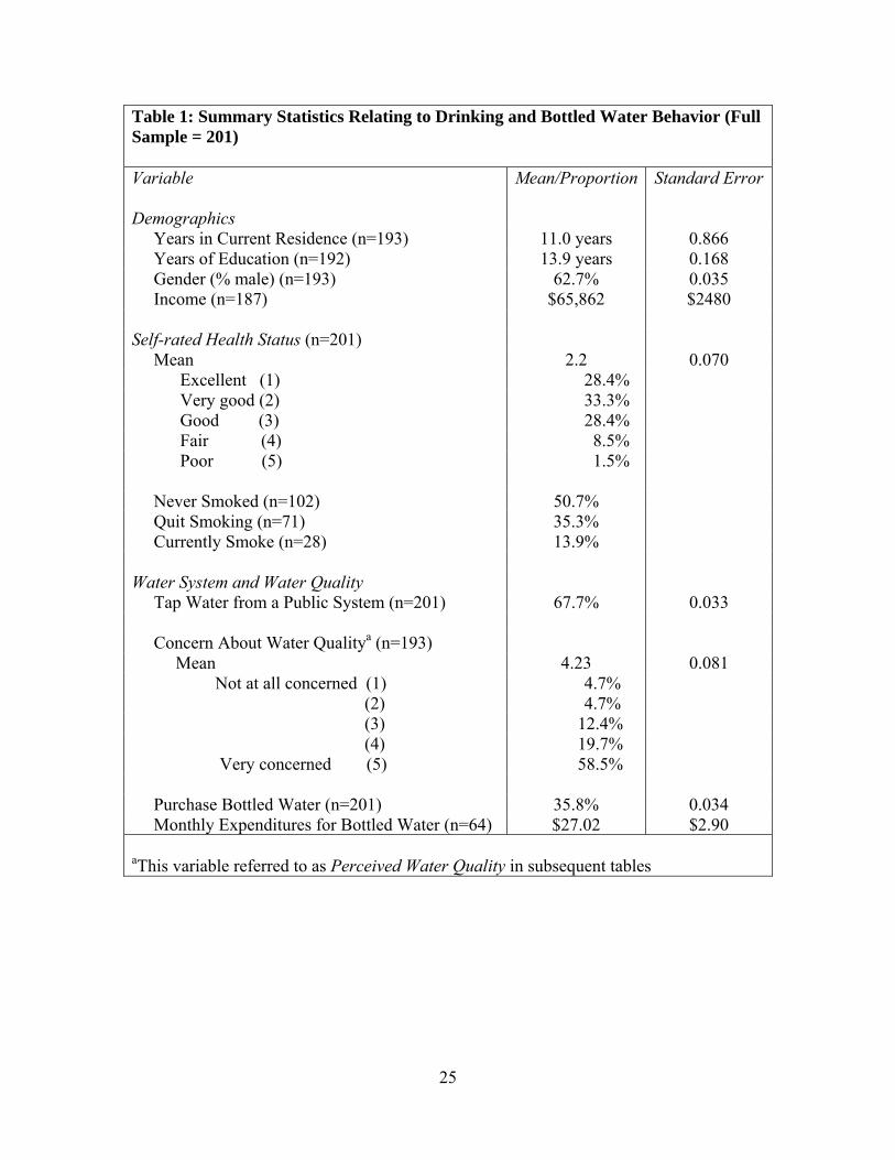
Table 1: Summary Statistics Relating to Drinking and Bottled Water Behavior (Full Sample = 201) Variable Demographics
Mean/Proportion Standard Error
Years in Current Residence (n=193) 11.0 years 0.866 Years of Education (n=192) 13.9 years 0.168 Gender (% male) (n=193) Income (n=187)
62.7% $65,862
0.035 $2480
Self-rated Health Status (n=201) Mean 2.2 0.070 Excellent (1) 28.4% Very good (2) 33.3% Good (3) 28.4% Fair (4) 8.5% Poor (5) 1.5% Never Smoked (n=102) 50.7% Quit Smoking (n=71) 35.3% Currently Smoke (n=28) 13.9% Water System and Water Quality Tap Water from a Public System (n=201) 67.7% 0.033 Concern About Water Qualitya (n=193) Mean 4.23 0.081 Not at all concerned (1) 4.7% (2) 4.7% (3) 12.4% (4) 19.7% Very concerned (5) 58.5% Purchase Bottled Water (n=201) 35.8% 0.034 Monthly Expenditures for Bottled Water (n=64) $27.02 $2.90
aThis variable referred to as Perceived Water Quality in subsequent tables
25
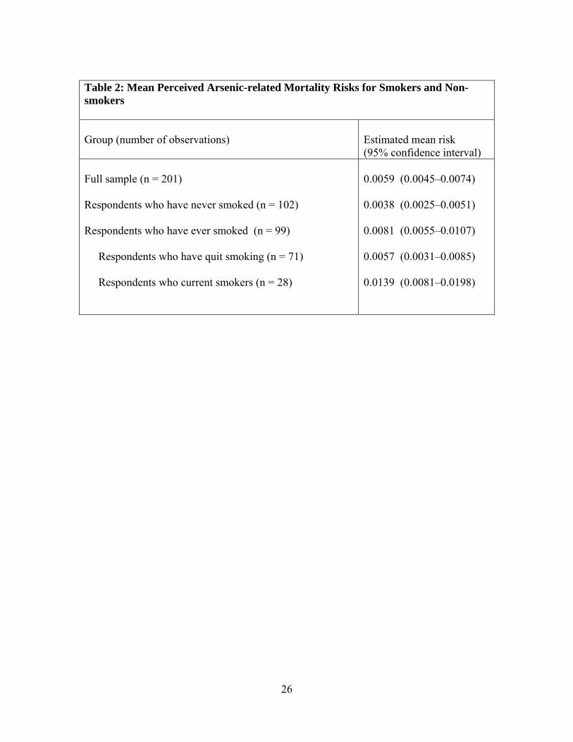
Table 2: Mean Perceived Arsenic-related Mortality Risks for Smokers and Non-smokers Group (number of observations)
Estimated mean risk (95% confidence interval)
Full sample (n = 201) Respondents who have never smoked (n = 102) Respondents who have ever smoked (n = 99) Respondents who have quit smoking (n = 71) Respondents who current smokers (n = 28)
0.0059 (0.0045–0.0074) 0.0038 (0.0025–0.0051) 0.0081 (0.0055–0.0107) 0.0057 (0.0031–0.0085) 0.0139 (0.0081–0.0198)
26
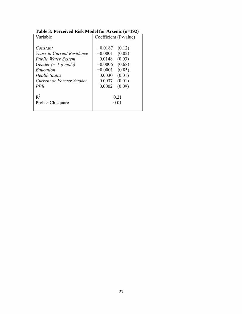
Table 3: Perceived Risk Model for Arsenic (n=192) Variable Constant Years in Current Residence Public Water System Gender (= 1 if male) Education Health Status
Current or Former Smoker PPB R2 Prob > Chisquare
Coefficient (P-value) −0.0187 (0.12) −0.0001 (0.02) 0.0148 (0.03) −0.0006 (0.68) −0.0001 (0.85) 0.0030 (0.01) 0.0037 (0.01) 0.0002 (0.09)
0.21 0.01
27
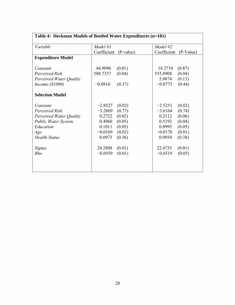
Table 4: Heckman Models of Bottled Water Expenditures (n=181) Variable Model #1
Coefficient (P-value) Model #2 Coefficient (P-Value)
Expenditure Model Constant Perceived Risk Perceived Water Quality Income ($1000) Selection Model Constant Perceived Risk Perceived Water Quality Public Water System Education Age Health Status Sigma Rho
44.9096 (0.01) 588.7337 (0.04) −0.0916 (0.37) −2.8527 (0.02) −3.2669 (0.77) 0.2722 (0.02) 0.4960 (0.05) 0.1011 (0.05) −0.0169 (0.02) 0.0973 (0.36) 24.2808 (0.01) −0.6939 (0.01)
18.2710 (0.87) 555.8908 (0.04) 5.0874 (0.13) −0.0773 (0.44) −2.5251 (0.02) −3.6164 (0.74) 0.2112 (0.06) 0.5192 (0.04) 0.0995 (0.05) −0.0178 (0.01) 0.0954 (0.38) 22.4733 (0.01) −0.6519 (0.05)
28
29
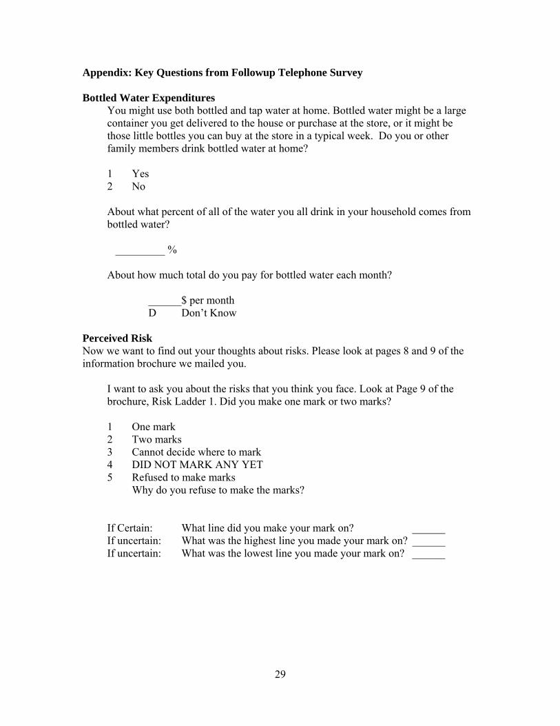
Appendix: Key Questions from Followup Telephone Survey Bottled Water Expenditures You might use both bottled and tap water at home. Bottled water might be a large
container you get delivered to the house or purchase at the store, or it might be those little bottles you can buy at the store in a typical week. Do you or other family members drink bottled water at home?
1 Yes 2 No
About what percent of all of the water you all drink in your household comes from
bottled water? _________ % About how much total do you pay for bottled water each month? ______$ per month
D Don’t Know Perceived Risk Now we want to find out your thoughts about risks. Please look at pages 8 and 9 of the information brochure we mailed you. I want to ask you about the risks that you think you face. Look at Page 9 of the
brochure, Risk Ladder 1. Did you make one mark or two marks?
1 One mark 2 Two marks 3 Cannot decide where to mark 4 DID NOT MARK ANY YET 5 Refused to make marks Why do you refuse to make the marks?
If Certain: What line did you make your mark on? ______ If uncertain: What was the highest line you made your mark on? ______ If uncertain: What was the lowest line you made your mark on? ______