Ritmico Progress, Rayney Wong Developing Process ... · Process Performance Baselines Process Performance Objectives Process Performance Models. November 19, 2008 Ritmico Progress

November 19, 2008 Ritmico Progress 1

Ritmico Progress, Ritmico Progress, RayneyRayney WongWong

DevelopingProcess Performance BaselinesProcess Performance ObjectivesProcess Performance Models


About the PresentationAbout the Presentation

About how a few companies at high maturity developed their PPB, PPO, PPM to meet business goals.

The companies performed project based software development.

Each company only has one type of methodology and life-cycle:

Iterative (Agile) or Waterfall.


About the PresentationAbout the Presentation

About how they took on a path that made high maturity acceptable by the staff.


Ritmico Progress, Ritmico Progress, RayneyRayney WongWong

Ritmico Progress is led by Rayney Wong who is a SCAMPI High Maturity lead appraiser, and a CMMI Introduction instructor. Ritmico Progress is a SEI Agreement Partner for the CMMI Product Suite and is a registered company in Singapore.

Rayney has over 20 years of software development and project management experience, ranging from radar communication systems, network systems, to publishing printer drivers and windows applications, and developing common coherent processes shared by offsite development centers.

Rayney's experience includes high maturity knowledge in developing models and Statistical process control toolkits, developing business strategic initiatives and staff development activities to achieve business goals, and training in implementing process improvements and software development. Companies have grown from 50 to over 500 people under Rayney’sguidance.

[email protected]

11/24/2008 NashLabs® 5

®

N A S H L A B O R A T O R I E S

® CMMI is registered in the U.S. Patent and Trademark Office by Carnegie Mellon University.

Since 1987 NashLabs® has helped Clients achieve a strategic advantage in the production of world-class software. We're focused on the measurement and improvement of software processes that work in the real world.

Nash Laboratories® is a Partner of the Software Engineering Institute at Carnegie-Mellon. As a Partner, the company is licensed to provide the latest generation of SEI technologies:

Introduction to the CMMI®

Introduction to the People-CMM®

SCAMPISM High-Maturity Appraisals

CMMI® Process Consulting

Six Sigma Training and Consulting

Rayney is an Associate with NashLabs®.

6

Shanghai 〇

BeiJing★

●Tokyu○

TianJin

BEIJING NTT DATA SYSTEMS INTEGRATION CO., LTD.

Founded in October 1, 1998Full Name: BEIJING NTT DATA SYSTEMS INTEGRATION CO., LTD.Location: BEIJING, CHINA, HeadquartersNumber of employees：640The main business

Off-shoring Software Development for JAPANSystem integration for Domestic business of CHINABusiness support for Domestic business of CHINA

Offshore development base in:BEIJING, SHANGHAI, TIANJINBeijing NTTDATA JAPAN: Sales/SE Dispatch etc

Main skills:Skill is widely distributed that covers open system trendsAcquisition of qualified skills: Oracle, MS systems, PMP

Project Management & Security – CMMI and ISO27001Image of the future: Current: off-shoring Software Development business.Future:

High Level off-shoring Software Development business.Service for the advance of Japanese Company into China MarketDomestic business of CHINARoll out Business for European and American enterprise

2400

3300

0

500

1000

1500

2000

2500

3000

3500

Mill

ion

Japa

n Y

en

1999 2000 2001 2002 2003 2004 2005 2006 2007 2008 2009

Sales TransitionOff-shoring

Intra-Mart

Business Support for China

Business for China

Future

650

800

0

100

200

300

400

500

600

700

800

1999 2000 2001 2002 2003 2004 2005 2006 2007 2008 2009

Growth (# of Employees)FutureBND JapanBND BeiJing

Core Service Provider

25 42 52 80 110 147 200 370 540 6501,200

2,300

3,700

5,000

1995

1996

1997

1998

1999

2000

2001

2002

2003

2004

2005

2006

2007

2008

E

Blue-Chip Customers

The People’s Bank of China

Publicly Listed on NYSE

December 12, 2007

Impressive Growth (Number of Employees)

Best-of-Breed Partners

Founded in 1995 - 13 year track record of working with global companies

Full Name: VanceInfo Technologies Inc.

Location: Beijing , Headquarter

NYSE: VIT First China based Outsourcing firm listed in US markets

Over 4500 diverse employees: 4412 developers

Substantial Global FootprintUSA (New York, Seattle, San Francisco), • China (Beijing, Shanghai , Nanjing, Tianjin, Hangzhou, Xian, Dalian

Chengdu, Shenzhen and Hong Kong) • Singapore & Japan• Australia (Melbourne)

Core capabilities• IT Services for Fortune 1000 companies and SMEs• Research & Development Services (Product Development)• Infrastructure Services • ITES/BPO

Domain knowledge & Vertical focus• Banking Financial Services and Insurance (BFSI)• Manufacturing & Retail & Distribution• Telecom• Technology

Centers of Excellence• Microsoft & Java• Enterprise Solutions: SAP, Oracle, PeopleSoft & Siebel• Business Intelligence & Data Warehousing• Messaging, EAI/B2Bi and SOA• QA & Testing Services

Quality delivery — CMMI and ISO certified

People Oriented Firm• Management Team with global experience• Voted “Top 100 Employers Most Favored by University Graduates”

VanceInfo Technologies Inc.

Perficient China Ltd.

Facts and HistoryPerficient’s Global Delivery Center was established in 2004130+ consultants -- 200 by EOY 2008Located in Hangzhou - Silicon Valley of ChinaAll business in Perficient China is conducted in EnglishAgile methodology delivering high priority requirements incrementally

Main BusinessWeb Application and Portal DevelopmentContent Management DevelopmentCRM / Siebel ImplementationSOA, Integration and Messaging ImplementationBPM Implementation

China Global Delivery Center


TerminologiesTerminologiesPPB Process-Performance Baselines

A documented characterization of the actual results achieved by following a process,

which is used as a benchmark for comparing actual process performance against

expected process performance.

PPO Quality and Process-Performance Objectives

Objectives and requirements for product quality, service quality, and process

performance. Process-performance objectives include quality; however, to emphasize the

importance of quality in the CMMI Product Suite, the phrase quality and

process-performance objectives is used rather than just process-performance objectives.

PPM Process-Performance Models

A description of the relationships among attributes of a process and its work products

that is developed from historical process-performance data and calibrated using collected

process and product measures from the project and that is used to predict results to be

achieved by following a process.

From SEI CMMI v1.2


TerminologiesTerminologies

From SEI CMMI v1.2

Base Measures

A distinct property or characteristic of an entity and the method for quantifying it. E.g.: Number of defects, Size of Module in KLoc (Thousand Lines of code)

Derived Measures

Data resulting from the mathematical function of two or more base measures. E.g.: Defect Density = (Number of Defects) / Module Size KLoc


BGS, VOPBGS, VOP--MARMAR

Purpose of all improvements are derived from the Business Goals Strategy (BGS).

Copyright Rayney Wong


VOPVOP--MARMAR


1 Vision Realizing and understanding the vision, breaking the vision down into its constituent parts.

2 Objectives Developing and prioritizing the goals and objectives that must be achieved to fulfill each part of the vision.

3 Problems Identifying and analyzing the problems and root causes that are preventing us from reaching the goals, objectives, and vision.

4 Measures Determining the measures to understand the extent of the problems and target measures to meet the objectives.

5 Actions Developing the actions for resolving the problems and reaching the goals. Improvements are aligned towards the objectives, vision and goals.

6 Risks Considering the side effects and costs of the actions in order to mitigate risks and side effects caused by the actions.

A BGS exercise typically takes up a period of several weeks and is performed annually.


BGS at High MaturityBGS at High Maturity



About the Measures in this PresentationAbout the Measures in this Presentation

Measures were from one of the companies.

Unit Testing of software modules with Test Cases.

Unit testing is performed after source codes have been reviewed:

Co-worker cross-check review of all source codes

Peer Review of critical module’s source codes

Measures have been adjusted by multiplying with factors as true measures cannot be shown.


PPB PPB –– Define the derived measures (part of BGS)Define the derived measures (part of BGS)

Unit Testing of software modules base measures:#Defects found by the developer during unit testing of his module.

Module code size in KLoc.

#Test cases used to unit test the module.

Total time in hours taken to test the module using the test cases.

Possible PPBs that can be derived:Defect Density = #Defects / Size KLoc

Test Case Density = #Test cases / Size KLoc

Test Speed = #Test cases / Testing time


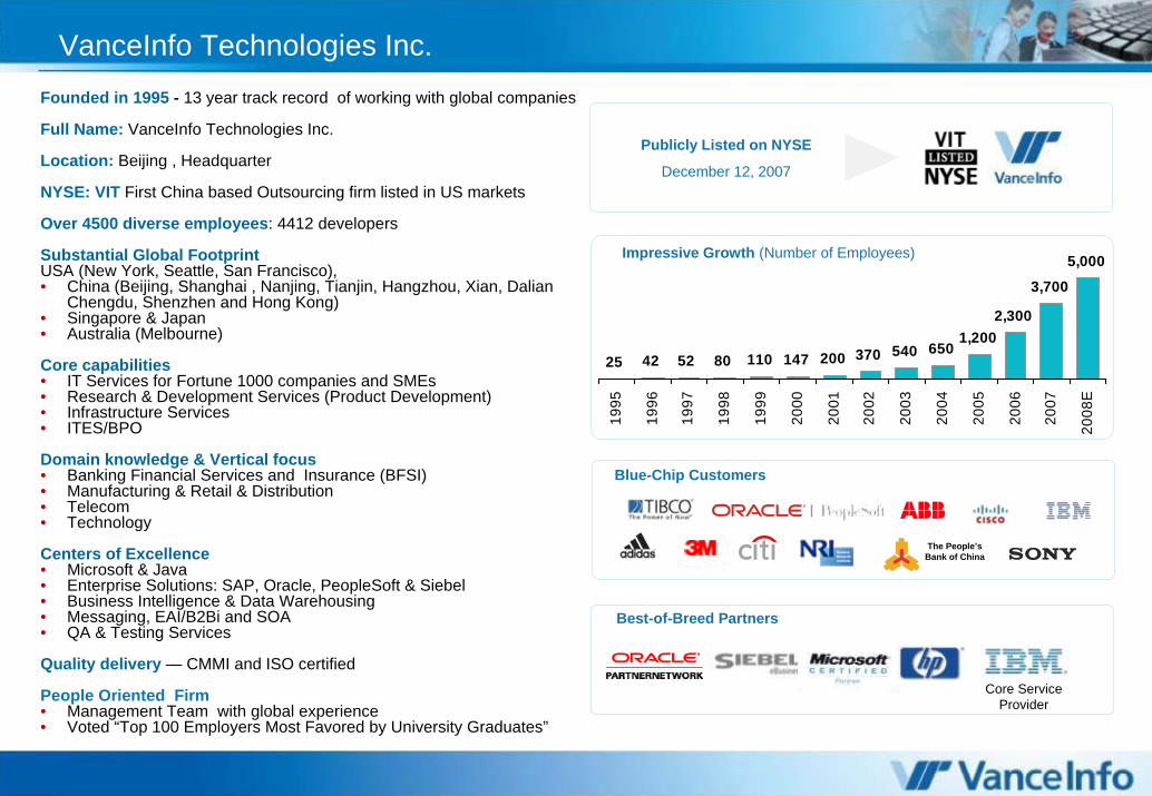
PPB PPB –– Perform Statistical AnalysisPerform Statistical Analysis

Defect Density for Unit TestingXmR or ImR requires time-sequenced data

#Defects/Size KLoc

PPB:UCL = 5.828

LCL = 0.833

Average of Group Items XmR

0

1

2

3

4

5

6

7

8

Index oftime-

sequencedY / X 10 20 30 40 50 60 70 80 90

Index

Gro

up It

em V

alue

# Defects

Code Size

KLOC

# Defects /Code Size

KLOC

59 15.6 3.782051282

57 27.8 2.050359712

54 20.4 2.647058824

77 18.2 4.230769231

84 24 3.5

18 7.6 2.368421053

56 18.4 3.043478261

95 25 3.8

20 10.78 1.85528757

32 7.8 4.102564103


PPB PPB –– When to Develop?When to Develop?

Data are added into the XmR control charts as soon as each Unit Testing of a module is performed.

How many data points before we can use the control charts?

XmR requires time-sequenced data.

X-Bar does not unless time-sequenced tests are performed.


False AlarmsFalse Alarms


33.5

38.5

43.5

48.5

53.5

58.51 2 3 4 5 6 7 8 9 10 11 12 13 14 15 16 17 18 19 20 21 22 23 24 25 26 27 28

Index

Gro

up It

em V

alue

Median of Group Items XmR

35

37

39

41

43

45

47

49

51

53

551 4 7 10 13 16 19 22 25 28 31 34 37 40 43 46 49 52 55 58 61 64 67 70 73 76 79

Index

Gro

up It

em V

alue

Item CL Average of ItemMedian of Item Item not included in limits calculationsItem not included in limits calculations

Drive with care. Small changes at a time.

Data shown are not from the organization.

For illustration purpose only.


Can Exception be removed?Can Exception be removed?Exception is found

Is it a problem inthe process?

Yes NoThis is an exception.Apply PreventiveCorrective Actions.

Is it a problem inthe product?

Yes No

Is this a commonproblem in the product? 5M, 1E?

Yes No Yes NoDo not remove exception if product problem cannotbe resolved. May require redesign in some modules.

This is an exception.Resolve problem inthe product.

This is an exception.Apply preventivecorrective actions.May require Training.

?Need more research?



0

1

2

3

4

5

6

7

8

Index oftime-

sequencedY / X 10 20 30 40 50 60 70 80 90

Index

Gro

up It

em V

alue

PPB PPB PPBPPB’’

For each exception or set of exceptions, perform a problem solving process to consider improvements to prevent them.

10% 20% 10%

5% 3%

100%

2% 5%

15% 20% 10%

Quantitative FishQuantitative Fish--Bone DiagramBone Diagram



Problem Solving Process must be done carefully to ensure improvements are able to prevent the exceptions.

Problem Solving Process are performed by the practitioners with guidance from the EPG.

Only remove the exceptions if there are improvements to prevent them.

0

10

20

30

40

50

60

C1 C2 C3 C4 C5 C6 C7

Category

Val

ue

0%

20%

40%

60%

80%

100%

120%

Cum

ulat

ive

Perc

entil

e



PPB’ is the improved PPB that the project may achieve after applying the improvements.

Processes, templates, checklists, training must be updated so that improvements permeate across the organization and become institutionalized.

With Pilot projects to confirm improvements.


PPB’PPB’

PPB’ of UT Defect Density (#Defects/Size KLoc)UCL = 5.601

LCL = 1.005

PPB earlier was:UCL = 5.828

LCL = 0.833


0

1

2

3

4

5

6

7

8

Index oftime-

sequencedY / X 11 22 33 44 55 66 77 88

Index

Gro

up It

em V

alue


PPB’ PPB’ PPO (before using PPM)PPO (before using PPM)

Each iteration’s PPB’ is used as the interim PPO for the next iteration or similar project.

PPB’ as PPO must be derived and calculated from adjustments to historical data, not by guesswork, and is therefore a realistic objective.

Average of Group It ems XmR

0

1

2

3

4

5

6

7

8

Index oftime-

sequencedY / X 12 24 36 48 60 72 84 96

Index

Gro

up It

em V

alue


0

1

2

3

4

5

6

7

8

Index oftime-

sequencedY / X 10 20 30 40 50 60 70 80 90

Index

Gro

up It

em V

alue


PPB’ PPB’ PPO (before using PPM)PPO (before using PPM)

Each subsequent iteration’s derived PPB and PPB’ gets better and better as improvements are continually and conscientiously applied by practitioners.

May not be for every iteration but for the overall project.Average of Group Items XmR

Index oftime-

sequencedY / X 11 22 33 44 55 66 77 88

Index

Gro

up It

em V

alue

Data shown are not from the organization.

For illustration purpose only.


PPOPPO (before using PPM)(before using PPM)

Each PPB’ incrementally progresses towards the VOB and VOC as improvements are continuously applied.

A process performance is therefore not immediately compared against its VOB or VOC.

Incremental calculated progress is planned with realistic timelines.


CorrelationCorrelation

Use PPB’ data to develop the correlations.

Begin with a simple two variable regression that the practitioners can see and feel.

Output Y: #Defects found in a module during UT

Input X: Module Size KLoc

Tool needs to be interactive.

Linear Model y = mx + b

# de

fect

s, Y

-axi

s

Code Size KLOC, X-axis

Linear Regression

y = 3.0399x + 2.8944R2 = 0.8222

-40

-20

0

20

40

60

80

100

120

0 5 10 15 20 25 30

Overall Average 0.00 Stdev around Overall Avg

Average predicted Y, linear line Confidence Interval

Prediction Interval Pred Y value

# defects / Code Size KLOC Not included # defects / Not included Code Size KLOC

Actual Y value Linear (# defects / Code Size KLOC)



Develop other correlations in separate regressions so that the practitioners can see how other variables affect the output Y.


Input X: #Test cases to test the module


# de

fect

s, Y

-axi

s

# UT Test Cases, X-axis

Linear Regression

y = 0.1106x + 2.7877R2 = 0.8155

-40

-20

0

20

40

60

80

100

120

0 100 200 300 400 500 600 700 800




# defects / # UT Test Cases Not included # defects / Not included # UT Test Cases

Actual Y value Linear (# defects / # UT Test Cases)



Exceptions or other data points that were removed would not be in the PPB’ correlations


Input X: Time spent to unit test the module


# de

fect

s, Y

-axi

s

UT Testing Time Hrs, X-axis

Linear Regression

y = 1.3858x + 8.5538R2 = 0.7073

-40

-20

0

20

40

60

80

100

120

140

0 10 20 30 40 50 60 70




# defects / UT Testing Time Hrs Not included # defects / Not included UT Testing Time Hrs

Actual Y value Linear (# defects / UT Testing Time Hrs)



Include other correlations to see how variables affect each other.

Output: #Test cases to test the module



X2:

# U

T Te

st C

ases

, Y-a

xis

X1: Code Size KLOC, X-axis

Linear Regression

y = 26.85x + 9.2348R2 = 0.9614

-100

0

100

200

300

400

500

600

700

800

900

0 5 10 15 20 25 30




X2: # UT Test Cases / X1: Code Size KLOC Not included X2: # UT Test Cases / Not included X1: Code Size KLOC

Actual Y value Linear (X2: # UT Test Cases / X1: Code Size KLOC)



Include other correlations to see how variables affect each other.

Output: Time spent to unit test the module

Input X: #Test cases to test the module


X3:

UT

Test

ing

Tim

e H

rs, Y

-axi

s

X2: # UT Test Cases, X-axis

Linear Regression

y = 0.0702x - 0.7941R2 = 0.894

-20

-10

0

10

20

30

40

50

60

70

0 100 200 300 400 500 600 700 800

Overall Average0.00 Stdev around Overall AvgAverage predicted Y, linear lineConfidence IntervalPrediction IntervalPred Y valueX3: UT Testing Time Hrs / X2: # UT Test CasesNot included X3: UT Testing Time Hrs / Not included X2: # UT Test CasesActual Y valueLinear (X3: UT Testing Time Hrs / X2: # UT Test Cases)


ModelingModeling

Later, include derived variables for modeling.

Output Y: #Defects found in a module during UT / Time Spent

Input X: #Test cases to test the module / Time Spent


#def

ects

/ U

T Te

stin

g Ti

me,

Y-a

xis

#UT Test Cases / UT Testing Time, X-axis

Linear Regression

y = 0.1616x - 0.6357R2 = 0.6121

-0.5

0

0.5

1

1.5

2

2.5

3

3.5

4

4.5

0 5 10 15 20 25 30

Overall Average0.00 Stdev around Overall AvgAverage predicted Y, linear lineConfidence IntervalPrediction IntervalPred Y value#defects / UT Testing Time / #UT Test Cases / UT Testing TimeNot included #defects / UT Testing Time / Not included #UT Test Cases / UT Testing TimeActual Y valueLinear (#defects / UT Testing Time / #UT Test Cases / UT Testing Time)



#def

ects

/ U

T Te

stin

g Ti

me,

Y-a

xis


Linear Regression

y = 0.1616x - 0.6357R2 = 0.6121

-0.5

0

0.5

1

1.5

2

2.5

3

3.5

4

4.5

0 5 10 15 20 25 30


ModelingModeling

Include other analysis as required

One standard deviation around the average




Frequency DistributionFrequency Distribution

Frequency distributionY/X

Y: #Defects found in a module during UT / Time Spent

X: #Test cases to test the module / Time Spent

Senior developers

Junior developers

Other tests of normality may be applied.

Frequency Distribution

0

5

10

15

20

25

0 0.05 0.1 0.15 0.2 0.25Group Item Value, X-axis

Freq

uenc

y C

ount

, Y-a

xis

Frequency Count of Y / X

UNPL from Average of Y / X

CL + 2 Sigma

CL + 1 Sigma

CL Average of Y / X

Median of Y / X

CL - 1 Sigma

CL - 2 Sigma

LNPL from Average of Y / X

Upper Specification Limit USL

Specification Center Line

Lower Specification Limit LSL



-1

0

1

2

3

4

5

Index oftime-

sequencedY / X 10 20 30 40 50 60 70 80 90

Index

Gro

up It

em V

alue

ExceptionsExceptions

There may be other exceptions to be improved.

Y/X

Y: #Defects found in a module during UT

X: Time spent to unit test the module


PPMPPM

When the practitioners are comfortable with the correlations, develop the multiple regression model using the Xn variables.

Y: # Defects X1: Code Size KLOC X2: # UT Test Cases X3: UT Testing Time Hrs59 15.6 455 22.8

57 27.8 605 54

54 20.4 593 39.6

77 18.2 398 29.4

84 24 697 46.2

18 7.6 209 16.2

56 18.4 403 23.4

95 25 734 47.4

20 10.78 294 21

32 7.8 225 17.4

Data shown are just part of the complete set.


PPMPPM

Y = 1.958602086*X1 + 0.059436937*X2 - 0.270573847*X3 + 2.251835318

Confidence Level 95.00% 0.05 AlphaConstant b set to zero? Non Zero

y=m1x1+m2x2+m3x3+…+b m1 m2 m3 bCoefficients 1.958602 0.059437 -0.27057 2.251835318 Constant b

Standard Errors for mn 0.74684 0.029757 0.221569 2.183538832 Standard error for bUpper 95.00% 3.44233 0.118555 0.169613 6.589816229Lower 95.00% 0.474874 0.000319 -0.71076 -2.086145592

R2 0.830087394 10.55925 Standard error for Y estimateF Statistics 146.5613558 90 df 1.5971E-34 F Distribution

ssreg 49023.8047 10034.8 ssresid

t-observed values 2.62252 1.9974 1.221169 1.03127789 1.986674497 t-criticalP-values 0.01025 0.048802 0.225211 0.305173947

Y: # Defects X1: Code Size KLOC X2: # UT Test Cases X3: UT Testing Time Hrs


Modeling improvedModeling improved

As more analysis is performed, practitioners may realize that a linear regression may not be the case for some variables correlation.



Polynomial X2 Model y = m2x2 + m1x + b

# de

fect

s, Y

-axi

s


Polynomial X2 Regression

y = -0.0448x2 + 4.3063x - 3.4798R2 = 0.8315

-40

-20

0

20

40

60

80

100

120

0 5 10 15 20 25 30


Average predicted Y, polynomial curve X2

Confidence Interval Upper Limit

Prediction Interval Upper Limit Pred Y value


Actual Y value Poly. (# defects / Code Size KLOC)


# de

fect

s, Y

-axi

s


Linear Regression

y = 3.0399x + 2.8944R2 = 0.8222

-40

-20

0

20

40

60

80

100

120

0 5 10 15 20 25 30








Greatest gradient is at 9 KLoc

Polynomial X2 Model y = m2x2 + m1x + b

# de

fect

s, Y

-axi

s



y = -0.0448x2 + 4.3063x - 3.4798R2 = 0.8315

-40

-20

0

20

40

60

80

100

120

0 5 10 15 20 25 30


Average predicted Y, polynomial curve X2

Confidence Interval Upper Limit

Prediction Interval Upper Limit Pred Y value


Actual Y value Poly. (# defects / Code Size KLOC)


# de

fect

s, Y

-axi

s


Linear Regression

y = 3.0399x + 2.8944R2 = 0.8222

-40

-20

0

20

40

60

80

100

120

0 5 10 15 20 25 30






Defects Code Size Defect Density

0.781777055 1 0.7817770554.953784418 2 2.4768922099.036253663 3 3.01208455413.02918479 4 3.25729619716.93257779 5 3.38651555920.74643268 6 3.4577387824.47074945 7 3.49582134928.10552809 8 3.51319101231.65076862 9 3.51675206935.10647103 10 3.51064710338.47263532 11 3.49751230241.74926149 12 3.47910512444.93634954 13 3.45664227348.03389947 14 3.4309928251.04191129 15 3.40279408653.96038498 16 3.37252406156.78932055 17 3.34054826859.52871801 18 3.30715162.17857734 19 3.27255670264.73889856 20 3.23694492867.20968166 21 3.20046103169.59092663 22 3.16322393871.88263349 23 3.12533189174.08480223 24 3.0868667676.19743285 25 3.04789731478.22052535 26 3.008481744





Polynomial X3 Model y = m3x3 + m2x

2 + m1x + b

#def

ects

/ U

T Te

stin

g Ti

me,

Y-a

xis



y = -0.0033x3 + 0.1634x2 - 2.4375x + 12.683R2 = 0.6837

0

0.5

1

1.5

2

2.5

3

3.5

4

0 5 10 15 20 25 30

Overall Average

0.00 Stdev around Overall Avg

Average predicted Y, polynomial curve X3Confidence Interval Upper Limit

Prediction Interval Upper Limit

Pred Y value

#defects / UT Testing Time / #UT Test Cases / UT Testing Time

Not included #defects / UT Testing Time / Not included #UT Test Cases / UT Testing Time

Actual Y value

Poly. (#defects / UT Testing Time / #UT Test Cases / UT Testing Time)


#def

ects

/ U

T Te

stin

g Ti

me,

Y-a

xis


Linear Regression

y = 0.1616x - 0.6357R2 = 0.6121

-0.5

0

0.5

1

1.5

2

2.5

3

3.5

4

4.5

0 5 10 15 20 25 30




Greatest gradient range:15 – 23 test cases per hour.

Polynomial X3 Model y = m3x3 + m2x

2 + m1x + b

#def

ects

/ U

T Te

stin

g Ti

me,

Y-a

xis



y = -0.0033x3 + 0.1634x2 - 2.4375x + 12.683R2 = 0.6837

0

0.5

1

1.5

2

2.5

3

3.5

4

0 5 10 15 20 25 30

Overall Average

0.00 Stdev around Overall Avg

Average predicted Y, polynomial curve X3Confidence Interval Upper Limit

Prediction Interval Upper Limit

Pred Y value

#defects / UT Testing Time / #UT Test Cases / UT Testing Time

Not included #defects / UT Testing Time / Not included #UT Test Cases / UT Testing Time

Actual Y value

Poly. (#defects / UT Testing Time / #UT Test Cases / UT Testing Time)


#def

ects

/ U

T Te

stin

g Ti

me,

Y-a

xis


Linear Regression

y = 0.1616x - 0.6357R2 = 0.6121

-0.5

0

0.5

1

1.5

2

2.5

3

3.5

4

4.5

0 5 10 15 20 25 30


Defects/ Testing Time

UT Test cases/ Testing time

Defects / UT Test Cases

1.347993798 10 0.134799381.24901571 11 0.113546883

1.258854477 12 0.104904541.357688464 13 0.1044375741.525696034 14 0.1089782881.743055554 15 0.1162037041.989945388 16 0.1243715872.246543901 17 0.1321496412.493029458 18 0.1385016372.709580423 19 0.1426094962.876375161 20 0.1438187582.973592038 21 0.1415996212.981409418 22 0.135518612.880005665 23 0.1252176382.649559146 24 0.1103982982.270248224 25 0.0908099291.722251265 26 0.0662404330.985746634 27 0.036509135


Modeling ImprovedModeling Improved

The residual of the polynomial X2 model should then be used in the XmR control chart to detect exceptions instead of Y/X.


-40

-30

-20

-10

0

10

20

30

40

Index oftime-

sequencedPolynomial

X2 13 26 39 52 65 78 91

Index

Gro

up It

em V

alue

# Defects Code SizeKLOC

# Defects /Code Size KLOC

Polynomial X2

Residual

59 15.6 3.782051282 6.196259923

57 27.8 2.050359712 -24.63645579

54 20.4 2.647058824 -11.73795637

77 18.2 4.230769231 16.93414707

84 24 3.5 9.91519777

18 7.6 2.368421053 -8.662361209

56 18.4 3.043478261 -4.599406317

95 25 3.8 18.80256715

20 10.78 1.85528757 -17.73976155

32 7.8 4.102564103 4.614264586


PPM improvedPPM improved

The preferred regression formula is used in the multiple regression:

Y:# Defects

Code Size KLOC

-0.0448X1^2 + 4.3063X1 - 3.4798

X2: # UTTest

Cases

X3: UTTesting

Time Hrs

59 52.80374 455 22.8

57 81.63646 605 54

54 65.73796 593 39.6

77 60.06585 398 29.4

84 74.0848 697 46.2

18 26.66236 209 16.2

56 60.59941 403 23.4

95 76.19743 734 47.4

20 37.73976 294 21

32 27.38574 225 17.4


PPMPPMY: # Defects Code Size KLOC

-0.0448X1^2 + 4.3063X1 - 3.4798 X2: # UT Test Cases X3: UT Testing Time Hrs

Confidence Level 95.00% 0.05 AlphaConstant b set to zero? Non Zero

y=m1x1+m2x2+m3x3+…+b m1 m2 m3 bCoefficients 0.065908 0.119684 -0.21865 2.054101583 Constant b

Standard Errors for mn 0.095014 0.018365 0.229078 2.40169675 Standard error for bUpper 95.00% 0.254669 0.15617 0.236454 6.825491266Lower 95.00% -0.12285 0.083197 -0.67375 -2.717288101


ssreg 48314.40909 10744.2 ssresid

t-observed values 0.693667 6.516767 0.954476 0.855271001 1.986674497 t-criticalP-values 0.489677 4.05E-09 0.342399 0.394672276

P-values did not improve so do not use the earlier regression formula for X1.


PPMPPM

Y = 1.912166199*X1 + 0.057942217*X2 -0.003927848*(X3)^2 + 0

Constant b (intercept) set to zero

90% confidence level. P-values have improved by using (X3)^2.

Y: # Defects X1: Code Size KLOC X2: # UT Test Cases X3: (UT Testing Time Hrs)^2

Confidence Level 90.00% 0.1 AlphaConstant b set to zero? Zero

y=m1x1+m2x2+m3x3+…+b m1 m2 m3 bCoefficients 1.912166 0.057942 -0.00393 0 Constant b

Standard Errors for mn 0.733273 0.027162 0.002075 #N/A Standard error for bUpper 90.00% 3.130698 0.103079 -0.00048 #N/ALower 90.00% 0.693634 0.012805 -0.00738 #N/A


ssreg 213662.4368 9954.563 ssresid

t-observed values 2.607713 2.133218 1.892992 #N/A 1.661771156 t-criticalP-values 0.010653 0.035598 0.061537 #N/A


Monte Carlo with XMonte Carlo with X33 as (Xas (X33)^2)^2

Simulation of the following:X1 ranges from 1 to 50 KLOC of Module Size

X2 ranges from >= 1 Test Cases

(Max test cases simulated was up to 1448, correlated with file size)

(X3)^2 ranges from >=1 Testing Time

(Max testing time simulated was up to 12624 hrs2, correlated with # test cases)

12624 hrs2 = (112.35 hrs)^2

100,000 simulations of 2,000 instances of UT

USL=5.601, LSL=1.005

Result: 97.4% >=LSL , 98.85% <= USL

96.25% within LSL and USL

Frequency Distribution

0

10

20

30

40

50

60

70

80

0 1 2 3 4 5 6Group Item Value, X-axis

Freq

uenc

y C

ount

, Y-a

xis

Frequency Count of DefectDensityY/X1

UNPL from Average of DefectDensityY/X1

CL + 2 Sigma

CL + 1 Sigma

CL Average of Defect DensityY/X1

Median of Defect DensityY/X1

CL - 1 Sigma

CL - 2 Sigma

LNPL from Average of DefectDensityY/X1





4

5

6

Index oftime-

sequencedDefectDensityY/X1 5 10 15 20 25 30 35 40 45 50 55 60 65 70 75 80 85 90 95 100

Index

m V

alu

0

1

2

3

Gro

up It

ee

USL Spec CL LSL Defect DensityY/X1



Item not included in limits calculations 14 points up and down

14 points above below CL Average 8 above below 1 sigma using Average 8 points above CL Average 8 points below CL Average

Trend of 6 points Increasing Trend of 6 points Decreasing 4 out of 5 points outside +1 sigma using Average 4 out of 5 points outside -1 sigma using Average

2 t f 3 P i t t id +2 Si i A 2 t f 3 P i t t id 2 Si i A O t id 3 Si i A N t i l d d Y / N t i l d d X

Data shown are of one instance of the simulation.


Optimum range of XOptimum range of X11: Code Size: Code Size

To ensure PPO can be achieved or exceeded

Arrange the input variables in the possible permutations (2n) of their reasonable minimum and maximum values

X1 X2 X3

0 0 00 0 10 1 00 1 11 0 01 0 11 1 01 1 1

Y = 1.912166199*X1 + 0.057942217*X2 -0.003927848*(X3)^2

Y: # Defects X1: Code Size

KLOC

X2: # UT Test Cases

X3: UT Testing Time Hrs^2

2.47587698 1 10 4Remove -ve Y 1 10 10000

88.8097803 1 1500 449.5470133 1 1500 1000096.1720207 50 10 456.9092537 50 10 10000182.505924 50 1500 4143.243157 50 1500 10000




Plot Y against X11: Code Size

Code Size is the most important controllable factor

Keep all file sizes <= 12 KLoc during planning of the modules’ WBS (work breakdown structure)

The higher the gradient, usually the higher the productivityCode Size

y = 18.59 Ln ( x ) + 46.94x =EXP (( y - 46.94) / 18.59)

45

65

85

105

125

145

165

185

205

0 10 20 30 40 50 60Code Size

Def

ects

X1: Code Size KLOC LSL USL Linear (X1: Code Size KLOC) Log. (X1: Code Size KLOC)



Code Size

y = 18.59 Ln ( x ) + 46.94x =EXP (( y - 46.94) / 18.59)

45

65

85

105

125

145

165

185

205

0 10 20 30 40 50 60Code Size

Def

ects


Defects Code Size

95.83397868 13.852849495.02715121 13.2647874894.22032373 12.7016891593.50146522 12.2201538393.48747921 12.2109684891.55774891 11.0075927990.42074775 10.3548599889.61403259 9.915349726

88.9882957 9.5873272188.66999985 9.42465758288.47703144 9.32738520486.95887644 8.59631125786.15204896 8.23139259485.34522148 7.8819649584.53839401 7.54737072483.73156653 7.22698022682.92473905 6.92019050182.11791157 6.626424188

81.3110841 6.34512843380.50425662 6.07577385679.69742914 5.81785354478.89060167 5.570882108


Monte Carlo with XMonte Carlo with X33 as (Xas (X33)^2 with Optimum Ranges)^2 with Optimum Ranges






3245 hrs2 = (57 hrs)^2


USL=5.601, LSL=1.005

Result: 99.95% >=LSL , 100% <= USL


Data shown are of one simulation.


Monte Carlo with XMonte Carlo with X33 as (Xas (X33)^2 with Optimum Ranges)^2 with Optimum RangesFrequency Distribution

0

5

10

15

20

25

0 1 2 3 4 5 6Group Item Value, X-axis

Freq

uenc

y C

ount

, Y-a

xis

Frequency Count of Defect DensityY/X1

UNPL from Average of Defect DensityY/X1

CL + 2 Sigma

CL + 1 Sigma



CL - 1 Sigma

CL - 2 Sigma

LNPL from Average of Defect DensityY/X1









0

1

2

3

4

5

6

Index oftime-

sequencedDefectDensityY/X1 5 10 15 20 25 30 35 40 45 50 55 60 65 70 75 80 85 90 95 100

Index

Gro

up It

em V

alue

USL Spec CL LSL Defect DensityY/X1



Item not included in limits calculations 14 points up and down

14 points above below CL Average 8 above below 1 sigma using Average 8 points above CL Average 8 points below CL Average

Trend of 6 points Increasing Trend of 6 points Decreasing 4 out of 5 points outside +1 sigma using Average 4 out of 5 points outside -1 sigma using Average

2 out of 3 Points outside +2 Sigma using Average 2 out of 3 Points outside -2 Sigma using Average Outside 3 Sigma using Average Not included Y / Not included X




Hypothesis Test for a Population Mean. If Null Hypothesis: mu varies, what happens to z ?

0

0.2

0.4

0.6

0.8

1

1.2

2.98 3.03 3.08 3.13 3.18 3.23 3.28

Null Hypothesis: mu defect density varies

P-va

lue

One

-Tai

led,

Tw

o-Ta

iled

-10

0

10

20

30

40

50

60

70

80

90

z St

anda

rd S

core

P-value Right-Tailed P-value Two-Tailed Null Hypothesis: mu <= 0.00, z is 84.2883 If z is zero, mu is X

What is mu if z is 1.96 ? What is mu if z is 1.64 ? Interval Lower Limit, t dist, X - Sampling error e Interval Upper Limit, t dist, X + Sampling error e

Standard Score z if mu varies X What is mu if z is -1.96 ?

95% confidence level of defect density: 3.07 – 3.22




Code Size

y = 18.59 Ln ( x ) + 46.94x =EXP (( y - 46.94) / 18.59)

45

65

85

105

125

145

165

185

205

0 10 20 30 40 50 60Code Size

Def

ects








11418 hrs2 = (106 hrs)^2


USL=5.601, LSL=1.005

Result: 99.95% >=LSL , 100% <= USL



Code Size

y = 18.59 Ln ( x ) + 46.94x =EXP (( y - 46.94) / 18.59)

45

65

85

105

125

145

165

185

205

0 10 20 30 40 50 60Code Size

Def

ects



Simulation of the following:In reality, there will be module Module Size of < 6

X1 ranges from 1 to 12 KLOC of Module Size





3273 hrs2 = (57.2 hrs)^2


USL=5.601, LSL=1.005

Result: 92.55% >=LSL , 96.85% <= USL



Code Size

y = 18.59 Ln ( x ) + 46.94x =EXP (( y - 46.94) / 18.59)

45

65

85

105

125

145

165

185

205

0 10 20 30 40 50 60Code Size

Def

ects








2725 hrs2 = (52.2 hrs)^2


USL=5.601, LSL=1.005

Result: 85.2% >=LSL , 93.8% <= USL

79% within LSL and USL


Code Size

y = 18.59 Ln ( x ) + 46.94x =EXP (( y - 46.94) / 18.59)

45

65

85

105

125

145

165

185

205

0 10 20 30 40 50 60Code Size

Def

ects



In the simulation of module size between 1 to 6, reasons for having many instances below LSL:

# of test cases was not enough or there were zero defects simulated.

Module Size Range KLOC 1 to 6 1 to 12 1 to 50 6 to 12 6 to 50LSL >= 85.20% 92.55% 97.40% 99.95% 99.95%<= USL 93.80% 96.85% 98.85% 100.00% 100.00%

Within LSL and USL 79.00% 89.40% 96.25% 99.95% 99.95%


X2:

# U

T Te

st C

ases

, Y-a

xis

X1: Code Size KLOC, X-axis

Linear Regression

y = 26.85x + 9.2348R2 = 0.9614

-100

0

100

200

300

400

500

600

700

800

900

0 5 10 15 20 25 30




X2: # UT Test Cases / X1: Code Size KLOC Not included X2: # UT Test Cases / Not included X1: Code Size KLOC

Actual Y value Linear (X2: # UT Test Cases / X1: Code Size KLOC)


Final DecisionFinal Decision

X1 ranges from 1 to 12 KLOC of Module SizeOnly a guideline, not an enforcement

6 KLOC was too stringent an upper limit, and

There will also be modules requiring < 6 KLOC, but

When breaking the modules into sub modules, aim for sub module size >= 6, E.g.:

Two sub modules, each 6 KLoc is better than (2, 10) or (3, 3, 3, 3)

Need practitioners to agree this makes sense

X2 Test Cases:Ensure there is enough, use the PPM for guidance

(X3)^2 Testing Time:Likewise, use the PPM for guidance



Simulated PPB ctrl limits:UCL = 5.92 defect density

LCL = 0.31

PPB’UCL = 5.601

LCL = 1.005

Need to also control:# Test Cases


Code Size

y = 18.59 Ln ( x ) + 46.94x =EXP (( y - 46.94) / 18.59)

45

65

85

105

125

145

165

185

205

0 10 20 30 40 50 60Code Size

Def

ects



Simulation of the following:In reality, there will be module Module Size of < 6

X1 ranges from 1 to 12 KLOC of Module Size





3273 hrs2 = (57.2 hrs)^2


USL=5.601, LSL=1.005

Result: 92.55% >=LSL , 96.85% <= USL



0

1

2

3

4

5

6

7

8

9

10

Index oftime-

sequencedY / X 5 10 15 20 25 30 35 40 45 50 55 60 65 70 75 80 85 90 95 100

Index

Gro

up It

em V

alue

USL Spec CL LSLY / X CL Average of Y / X Median of Y / XItem not included in limits calculations 14 points up and down 14 points above below CL Average8 above below 1 sigma using Average 8 points above CL Average 8 points below CL AverageTrend of 6 points Increasing Trend of 6 points Decreasing 4 out of 5 points outside +1 sigma using Average4 out of 5 points outside -1 sigma using Average 2 out of 3 Points outside +2 Sigma using Average 2 out of 3 Points outside -2 Sigma using AverageOutside 3 Sigma using Average Not included Y: # Defects / Not included X1: Code Size KLOC



Module size from 1 to 12 KLoc

Test Cases variation : Calculated + - 50

Testing time variation : Calculated + - 10 hrs

Simulated PPB ctrl limits:UCL = 4.86 defect density

LCL = 2.12

PPB’UCL = 5.601

LCL = 1.005


0

1

2

3

4

5

6

7

Index oftime-

sequencedY / X 5 10 15 20 25 30 35 40 45 50 55 60 65 70 75 80 85 90 95 100

Index

Gro

up It

em V

alue

USL Spec CL LSLY / X CL Average of Y / X Median of Y / XItem not included in limits calculations 14 points up and down 14 points above below CL Average8 above below 1 sigma using Average 8 points above CL Average 8 points below CL AverageTrend of 6 points Increasing Trend of 6 points Decreasing 4 out of 5 points outside +1 sigma using Average4 out of 5 points outside -1 sigma using Average 2 out of 3 Points outside +2 Sigma using Average 2 out of 3 Points outside -2 Sigma using AverageOutside 3 Sigma using Average Not included Y: # Defects / Not included X1: Code Size KLOC


E.g. Module Size 9 E.g. Module Size 9 KLocKLocSize of module (KLoc): 9

QPPO USL 5.601 50.409

QPPO LSL 1.005 9.045

Y: # Defects

X1: Code Size

KLOC

X2: # UT Test Cases

(Ideal)

X3: UT Testing Time Hrs^2 (Ideal)

X3: UT Testing

Time Hrs (Ideal)

30.63356 9 250.8809 283.2419 16.82979# UT Test Cases = (26.85* module code size + 9.23)

UT Testing Time2 =(0.07* Test Cases - 0.79)^2

y = m1x1 + m2x2 + m3x3 + b m1 m2 m3 bCoefficients 1.912166 0.057942 -0.00393 0

Y: # Defects

X1: Code Size

KLOC

X2: # UT Test Cases

(min, max)

X3: UT Testing Time Hrs^2 (min, max)

X3: UT Testing

Time Hrs (min, max)

17.26351 9 1 1 13.638934 9 1 3469.713 58.9042775.35195 9 1003.524 1 161.72737 9 1003.524 3469.713 58.90427

Expected defects to be found according to PPO and size of module


E.g. Module Size 9 E.g. Module Size 9 KLocKLoc

81.95% USL — LSL

Module code size9 KLoc

UT Test Cases1 – 1003

UT Testing Time1 – 81 hrs

PPO is too wideCommon problems

UT Test Cases

0

20

40

60

80

0 200 400 600 800 1000 1200UT Test Cases

# D

efec

ts

Y: # Defects Simulated PPO USL #defectsPPO LSL #defects X2: # UT Test Cases (min, max)X2: # UT Test Cases (Ideal) Best Case USL #defectsBest Case LSL #defects

UT Testing Time

01020304050607080

0 10 20 30 40 50 60 70 80 90UT Testing Time

# D

efec

tsX3: UT Testing Time Hrs Simulated PPO USL #defectsPPO LSL #defects X3: UT Testing Time Hrs (min, max)X3: UT Testing Time Hrs (Ideal) Best Case USL #defectsBest Case LSL #defects


E.g. Module Size 9 E.g. Module Size 9 KLocKLoc

100% USL — LSL

Module code size9 KLoc

UT Test Cases200 – 300

UT Testing Time9 – 22 hrs

UT Test Cases

0

20

40

60

80

0 200 400 600 800 1000 1200UT Test Cases

# D

efec

ts

Y: # Defects Simulated PPO USL #defectsPPO LSL #defects X2: # UT Test Cases (min, max)X2: # UT Test Cases (Ideal) Best Case USL #defectsBest Case LSL #defects

UT Testing Time

0

20

40

60

80

0 10 20 30 40 50 60 70UT Testing Time

# D

efec

tsX3: UT Testing Time Hrs Simulated PPO USL #defectsPPO LSL #defects X3: UT Testing Time Hrs (min, max)X3: UT Testing Time Hrs (Ideal) Best Case USL #defectsBest Case LSL #defects


Composing the Defined ProcessComposing the Defined ProcessAverage of Group Items XmR

0

1

2

3

4

5

6

7

8

Index oftime-

sequencedY / X 12 24 36 48 60 72 84 96

Index

Gro

up It

em V

alue


0

1

2

3

4

5

6

7

8

Index oftime-

sequencedY / X 10 20 30 40 50 60 70 80 90

Index

Gro

up It

em V

alue

Project

PPB PPB’

PPO

Next Iteration

PPB PPB’

Compare

Next Iteration

PPM PPM’

PPO

PPM PPM’


#def

ects

/ UT

Testi

ng T

ime,

Y-a

xis


Linear Regression

y = 0.1616x - 0.6357R2 = 0.6121

-0.5

0

0.5

1

1.5

2

2.5

3

3.5

4

4.5

0 5 10 15 20 25 30



#def

ects

/ U

T Te

stin

g Ti

me,

Y-a

xis


Linear Regression

y = 0.1616x - 0.6357R2 = 0.6121

-0.5

0

0.5

1

1.5

2

2.5

3

3.5

4

4.5

0 5 10 15 20 25 30


Org PPM

Org PPM


Process Performance parameters ConsiderationsProcess Performance parameters Considerations


Unit Testing Process possible parametersUnit Testing Process possible parameters

Process Parameters:Test effort#Test casesTest case complexityTester training type, time, effectivenessTested FrequencyTester Experience

Output:#Defects FoundTest Coverage %Remaining #defects

Product Parameters:Product Module sizeProgramming languageProduct Module complexity#Changes LOCRework EffortAuthor ExperienceModule development effort

Standards:Test case densityProduct standardsTest case guidelines

Interacting Process:#SQA audit on writing the test cases#Non-compliances found by QATest case review time#Issues found in test case review

Unit Testing Process

Equipment, Tools, Environment:Tools:-WinRunner-LoadRunnerMethods:-White box testing-Black box testing

Take care of discrete variables which cannot be used in multiple regression.


UT Testing ProcessUT Testing Process

Selected parameters:Y = #Test Defects Found

X1 = Test Effort - controllable

X2 = #Test Cases – controllable during planning

X3 = Tested Frequency (# times tested) - controllable

X4 = Product module size – controllable during planning

X5 = Development Effort – need more consideration


Questions?Questions?

Ritmico Progress, Rayney Wong

[email protected]

Documents

Ritmico Progress, Rayney Wong Developing Process ... · Process Performance Baselines Process Performance Objectives Process Performance Models. November 19, 2008 Ritmico Progress