Ritz values - Computational and Applied Mathematicsembree/87269.pdf · SIAM J. MATRIX ANAL. APPL. c 2012 Society for Industrial and Applied Mathematics Vol. 33, No. 4, pp. 1320–1338

SIAM J. MATRIX ANAL. APPL. c© 2012 Society for Industrial and Applied MathematicsVol. 33, No. 4, pp. 1320–1338

RITZ VALUE LOCALIZATION FOR NON-HERMITIAN MATRICES∗

RUSSELL L. CARDEN† AND MARK EMBREE†

Abstract. Rayleigh–Ritz eigenvalue estimates for Hermitian matrices obey Cauchy interlacing,which has helpful implications for theory, applications, and algorithms. In contrast, few resultsabout the Ritz values of non-Hermitian matrices are known, beyond their containment within thenumerical range. To show that such Ritz values enjoy considerable structure, we establish regionswithin the numerical range in which certain Ritz values of general matrices must be contained. Todemonstrate that localization occurs even for extreme examples, we carefully analyze possible Ritzvalue combinations for a three-dimensional Jordan block.

Key words. Ritz values, numerical range, inverse field of values problem

AMS subject classifications. 15A18, 15A42, 47A10, 65F15

DOI. 10.1137/120872693

1. Introduction. Rayleigh–Ritz eigenvalue estimates arise throughout appliedmathematics, facilitating the analysis of physical systems and enabling a variety ofcomputational algorithms. For example, iterative methods for solving large linearsystems and eigenvalue problems rely fundamentally on Ritz values and their harmonicvariants. One cannot fully comprehend the behavior of these algorithms, nor see howbest to accelerate their convergence, without deeply understanding Ritz values.

Consider a matrix A ∈ Cn×n and a p-dimensional subspace V ⊂ Cn, and let thecolumns of V ∈ Cn×p form an orthonormal basis for V. Hence Ran(V) = V, whereRan(·) denotes the range (column space) of a matrix. The eigenvalues of V∗AV arecalled the Ritz values of A with respect to V. These values are independent of theorthonormal basis V for V.

After more than a century of study much is known about the Ritz values of Her-mitian matrices (and self-adjoint operators in Hilbert space). Among the earliest andmost descriptive results for matrices is the Cauchy interlacing theorem; see, e.g., [15].Suppose A is Hermitian with eigenvalues λ1 ≤ λ2 ≤ · · · ≤ λn. Then V∗AV isHermitian, so its eigenvalues—the Ritz values of A with respect to V—are also real:θ1 ≤ θ2 ≤ · · · ≤ θp. The Cauchy interlacing theorem gives

θk ∈ [λk, λn+k−p], k = 1, . . . , p.

Beyond the Hermitian case, our understanding remains surprisingly primitive. Recentwork provides insight for normal matrices, including a geometric description of theRitz values for p = n − 1 [5, 13], and a characterization of Ritz values from Krylovsubspaces [2]. For general matrices, little has been said beyond the tautology that allRitz values must fall within the numerical range (field of values)

W (A) := {v∗Av : v ∈ Cn, ‖v‖ = 1},

which is simply the set of all Ritz values. For p = 1, several recently proposed algo-rithms identify subspaces that generate any given θ1 ∈ W (A), the so-called inverse

∗Received by the editors April 9, 2012; accepted for publication (in revised form) by J. BarlowSeptember 26, 2012; published electronically December 12, 2012. Supported by National ScienceFoundation grant DMS-CAREER-0449973.

http://www.siam.org/journals/simax/33-4/87269.html†Department of Computational and Applied Mathematics, Rice University, Houston, TX 77005–

1892 ([email protected], [email protected]).

1320

RITZ VALUE LOCALIZATION FOR NON-HERMITIAN MATRICES 1321

field of values problem [3, 6, 20]. For subspaces of dimension p > 1 this problem ismuch more difficult; indeed, given two points θ1, θ2 ∈ W (A), no satisfactory methodis known to verify whether there exists any two-dimensional subspace V ⊂ Cn thatgives both θ1 and θ2 as Ritz values. In general, the problem of identifying thosesets {θ1, . . . , θp} ⊂ W (A) that can be realized as Ritz values from a p-dimensionalsubspace, along with that generating subspace, is known as the iFOV(p) problem [3].We seek to understand this problem for 2 ≤ p ≤ n − 1. Absent such insight, wecan summarize the state of the art as follows: little, if anything, is known about the“inner geometry” [20] of the numerical range for nonnormal A.

This situation has unfortunate consequences, complicating eigenvalue estimationfor non-self-adjoint operators (as motivated by problems in physics and engineering)and preventing a deep understanding of iterative methods for large-scale linear sys-tems and eigenvalue problems. Indeed the latter motivated our present study. We wishto analyze the convergence of Sorensen’s implicitly restarted Arnoldi algorithm [19],a leading method for computing eigenvalues of large, sparse matrices that is imple-mented in the ARPACK software package [12] and MATLAB’s eigs command. Thisalgorithm develops approximations to invariant subspaces of A from Krylov subspaceswhose starting vectors are repeatedly refined through application of a filter polyno-mial. The standard “exact shift” procedure identifies the Ritz values that most closelyresemble the desired eigenvalues (e.g., the rightmost eigenvalues), then uses the re-maining Ritz values as roots of the filter polynomial. This process will fail when oneof these roots coincides with a desired eigenvalue, effectively deflating that eigenvaluefrom the approximating subspace [7]. A satisfactory convergence theory that accountsfor such cases must rely on fine properties of the Ritz values.

This work began with an experiment that precisely illustrates how some gener-alization of “interlacing”—that is, a geometric restriction on the location of certainRitz values—can hold even for the antithesis of the well-understood Hermitian case.Take A to be the 3× 3 Jordan block

A =

⎡⎣ 0 1 00 0 10 0 0

⎤⎦ .(1.1)

It is well known that W (A) = {z ∈ C : |z| ≤ √2/2}, the closed disk of radius

√2/2

in the complex plane, centered at the origin [8, p. 9]. Now generate random two-dimensional (complex) subspaces, compute the Ritz values, and sort them by theirreal parts. Figure 1.1 illustrates the results: the leftmost Ritz values appear to coveronly a portion of the numerical range. In none of these 10,000 experiments does theleftmost Ritz value fall near the rightmost extent of W (A); for example, it appearsto be impossible for both Ritz values to fall near the point z = 1/2.

This observation is easy to confirm analytically, at least in a coarse manner. LetV be a two-dimensional subspace of C3 that is spanned by the orthonormal basis{v1,v2}. Construct the matrix V = [v1,v2], and let v3 be a unit vector orthogonalto V, so that U = [v1,v2,v3] ∈ C3×3 is unitary and the eigenvalues of V∗AV are theRitz values θ1 and θ2 of A from V. Letting tr(·) denote the trace, notice that

0 = tr(A) = tr(U∗AU) = tr(V∗AV) + v∗3Av3 = θ1 + θ2 + v∗

3Av3.

Label the leftmost Ritz value as θ1, so Re(θ1) ≤ Re(θ2). Since v∗3Av3 ∈W (A),

Re(θ1) = −Re(v∗3Av3)− Re(θ2) ≤

√2

2− Re(θ1),

1322 RUSSELL L. CARDEN AND MARK EMBREE

−0.75 −0.5 −0.25 0 0.25 0.5 0.75

−0.75

−0.5

−0.25

0

0.25

0.5

0.75

−0.75 −0.5 −0.25 0 0.25 0.5 0.75

−0.75

−0.5

−0.25

0

0.25

0.5

0.75

Fig. 1.1. Ritz values drawn from 10,000 random two-dimensional subspaces of C3. Each pairof Ritz values is sorted by real part: the leftmost Ritz value from each experiment is shown on theleft, while the rightmost Ritz value is plotted on the right. In both cases the solid circle denotes theboundary of W (A), while the vertical lines indicate the upper bound on the leftmost Ritz value (1.2)and the analogous lower bound on the rightmost Ritz value.

from which we conclude that

Re(θ1) ≤√2

4.(1.2)

This bound and the analogous lower bound −√2/4 ≤ Re(θ2) are shown as vertical

lines in Figure 1.1.In the spirit of these simple bounds, we establish in the next section containment

regions that “localize” the Ritz values of general matrices. While not as sharp asCauchy interlacing for Hermitian matrices, these bounds do reveal considerable “innergeometry” within the numerical range. We later give more detailed analysis for p = 2Ritz values of a 3 × 3 Jordan block, which reveals the additional structure hinted atin Figure 1.1 and indicates the challenge of completely understanding Ritz values forgeneral matrices. To the best of our knowledge, this is the first work to preciselyanalyze the Ritz values of any nonnormal matrix.

2. Ritz values of general matrices. The simple bound (1.2) on the rightmostextent of the leftmost Ritz value for a three-dimensional Jordan block, derived usinga trace argument, is a special case of more general analysis based on eigenvalue ma-jorization. In this section, we develop bounds on the Ritz values, sorted by real partand magnitude. Such bounds are useful for stability analysis of dynamical systems,where one seeks rightmost eigenvalues for continuous time systems and largest mag-nitude eigenvalues for discrete time systems. For similar bounds on the phases of Ritzvalues, see [4, section 3.2.2].

2.1. Bounds on the real part of Ritz values. Any matrix A ∈ Cn×n can be

decomposed into the sum of its Hermitian and skew-Hermitian parts, H := (A+A∗)/2and S := (A −A∗)/2i; some call A = H+ iS the Cartesian decomposition [17]. Wewish to study the Ritz values of A drawn from the p-dimensional subspace Ran(V),where V ∈ Cn×p has orthonormal columns. Without loss of generality, assume thisbasis is chosen in such a way that V∗AV is upper triangular (via the Schur decompo-sition), and hence the Ritz values are on its main diagonal. Label them by increasing


real part: Re θ1 ≤ Re θ2 ≤ · · · ≤ Re θp. Let the columns of V ∈ Cn×(n−p) form anorthonormal basis for the orthogonal complement of Ran(V), which can always be

done in a manner that makes V∗AV ∈ C(n−p)×(n−p) upper triangular. Label theeigenvalues of V∗AV as θp+1, . . . , θn. The set Θ := {θ1, θ2, . . . , θn} comprises the

diagonal entries of [V V]∗A[V V], while the real parts Re θ1,Re θ2, . . . ,Re θn are the

diagonal entries of [V V]∗H [V V].Now let μ1 ≤ μ2 ≤ · · · ≤ μn denote the eigenvalues of H, and relabel the members

of Θ by increasing real part: Re θ(1) ≤ Re θ(2) ≤ · · · ≤ Re θ(n). By a classical result of

Schur [1, p. 35], the vector [Re θ(j)]nj=1 of (ordered) diagonal entries of [V V]∗H[V V]

majorizes the vector [μj ]nj=1 of eigenvalues, i.e.,

k∑j=1

μj ≤k∑

j=1

Re θ(j), k = 1, . . . , n,

with equality for k = n. Since Re θ(j) ≤ Re θj , we have

k∑j=1

μj ≤k∑

j=1

Re θj , k = 1, . . . , p,(2.1)

which means that the vector [Re θj ]pj=1 weakly majorizes the vector [μj ]

pj=1. From

this majorization one can derive bounds that localize where the Ritz values θj of Amust fall in the complex plane. For example, the weak majorization (2.1) with k = 2implies

μ1 + μ2 ≤ Re θ1 +Re θ2 ≤ 2Re θ2,

and so

μ1 + μ2

2≤ Re θ2,

restricting the leftmost extent of the second Ritz value of A. For the kth Ritz value,

μ1 + · · ·+ μk ≤ Re θ1 + · · ·+Re θk ≤ kRe θk.(2.2)

Applying the analysis to −A yields

μn−p+k + · · ·+ μn ≥ Re θk + · · ·+Re θp ≥ (p− k + 1)Re θk.

These bounds are summarized in the following theorem. The idea of majorizing thereal part of the spectrum by the spectrum of H dates back to Ky Fan in the 1950s[1, Proposition III.5.3], [14, section 9.F], though we are unaware of previous use ofthis fact to bound Ritz values.

Theorem 2.1. Let θ1, . . . , θp denote the Ritz values of A ∈ Cn×n drawn froma p < n dimensional subspace, labeled by increasing real part: Re θ1 ≤ · · · ≤ Re θp.Then for k = 1, . . . , p,

μ1 + · · ·+ μk

k≤ Re θk ≤ μn−p+k + · · ·+ μn

p− k + 1,(2.3)

where μ1 ≤ · · · ≤ μn are the eigenvalues of H = 12 (A+A∗).


Corollary 2.2. At most m < p Ritz values of A ∈ Cn×n from a p-dimensionalsubspace can be contained in each of the following subsets of the complex plane:

Ω�,m := {z ∈W (A) : Re z ∈ [�m, �m+1)},Ωr,m := {z ∈W (A) : Re z ∈ (rm+1, rm]},

where, for k = 1, . . . , p,

�k :=μ1 + · · ·+ μk

k, rk :=

μn−k+1 + · · ·+ μn

k.

For k = 1 and k = p, (2.3) yields the trivial statement

μ1 ≤ Re θ1 ≤ Re θp ≤ μn,

which more directly follows from the fact that Ritz values are in the numerical range,and Re(W (A)) = [μ1, μn]. For k ∈ {2, . . . , p− 1}, the theorem can provide consider-able insight into the interior structure of the numerical range. We shall examine thisin more detail for Jordan blocks at the end of this section.

Is Theorem 2.1 sharp? If A is Hermitian, then H = A, and μ1, . . . , μn are theeigenvalues of A. One can immediately compare Theorem 2.1 to the bounds from theCauchy interlacing theorem:

μk ≤ θk ≤ μn−p+k.

The Cauchy bounds, which can always be attained, will be considerably tighter thanTheorem 2.1 when the eigenvalues of A = H are well separated.

The slack in Theorem 2.1 can be attributed to the second inequality in (2.2), forthe majorization in (2.1) becomes strong (i.e., with equality for k = p), when thesubspace Ran(V) corresponds to the eigenspace for the p smallest eigenvalues of H.If the eigenvalues of the Hermitian part are distinct, the corresponding subspaces areunique.1 To obtain sharper bounds, one could draw in further information about thenumerical range, e.g., based on the skew-Hermitian part of A. (Recently Psarrakosand Tsatsomeros have used the second largest eigenvalue of H to develop inclusionregions for the spectrum [16].)

2.2. Illustration: Jordan blocks. When A is an n-dimensional Jordan block(ones on the first superdiagonal, zeros elsewhere), we can compute the bounds inTheorem 2.1 explicitly. In this case

H =1

2

⎡⎢⎢⎢⎣0 1

1 0. . .

. . .. . . 11 0

⎤⎥⎥⎥⎦has well-known eigenvalues

μj = cos((n− j + 1)π

n+ 1

), j = 1, . . . , n;

1For the n = 3 Jordan block, this is precisely why the left plot in Figure 1.1 suggests thatonly two points (complex conjugates) might attain the bound Re θ1 ≤ √

2/4. In this case, takeRan(V) to be the eigenspace of H corresponding to μ2 and μ3. Then W (V∗AV) is an ellipse (sinceV∗AV ∈ C2×2; see [10, section 1.3]) with minor axis [0,

√2/2] = [μ2, μ3]. The Ritz values are

(√2±√

2i)/4, attaining the bound Re θ1 ≤ √2/4.


−1 −0.8 −0.6 −0.4 −0.2 0 0.2 0.4 0.6 0.8 1

1

2

3

4

5

6

7

Re θk

index

,k

Fig. 2.1. Theorem 2.1 illustrated for a Jordan block of dimension n = 8. For each of k =1, . . . , n− 1, the bound from Theorem 2.1 is shown as a bracket containing the real parts of the Ritzvalues θk drawn from 2000 random real p = n− 1 dimensional subspaces (solid black dots).

n = 2 n = 4 n = 8 n = 16 n = 32

Fig. 2.2. Containment regions (gray) for the rightmost eigenvalue θn−1 of an n × n Jordanblock drawn from a p = n − 1 dimensional subspace, based on Theorem 2.1. (The circles mark theboundaries of the numerical range.)

see [8, section 1.3] for a discussion of the numerical range of this A. Figure 2.1illustrates Theorem 2.1 for p = 7 dimensional subspaces for the Jordan block withn = 8.

For Jordan blocks of dimension n, tr(H) = 0 implies that μ1+ · · ·+μn−1 = −μn,so for p = n− 1,

Re θn−1 ≥ − 1

n− 1μn = − 1

n− 1cos( π

n+ 1

)≥ − 1

n− 1.

The numerical range W (A) comprises the disk of radius cos(π/(n+1)); Theorem 2.1establishes a containment region for the rightmost Ritz value θn−1 that tends towardthe right half of W (A); see Figure 2.2. It might initially seem surprising that thisbound does not require the rightmost Ritz value from a p = n−1 dimensional subspaceto fall further to the right. However, if we take for V the first n − 1 columns of then×n identity matrix, then V∗AV is the (n−1)× (n−1) upper-left corner of A. Thecorresponding Ritz values are θ1 = θ2 = · · · = θn−1 = 0: hence any bound on Re θn−1

must contain the interval [0, cos(π/(n + 1))]. Rightmost Ritz values with small real


parts might be rare in practice (as indicated in the random samples in Figure 2.1),but general bounds must account for them.

To illustrate how Theorem 2.1 reveals some “inner geometry” of the numericalrange, consider one more numerical experiment. We construct three nondiagonalizablematrices of dimension n = 8 that have the same numerical range; this implies that theextreme eigenvalues of the Hermitian parts are identical. However, we pick the matrixentries so the interior eigenvalues of the Hermitian parts are quite different. We takeA2 to be the 8 × 8 Jordan block studied previously, with ones on the superdiagonal.Then consider the matrices

A1 := γ1

⎡⎢⎢⎢⎢⎢⎢⎢⎢⎢⎣

0 10 0

0 10 0

0 10 0

0 10 0

⎤⎥⎥⎥⎥⎥⎥⎥⎥⎥⎦, A3 := γ3

⎡⎢⎢⎢⎢⎢⎢⎢⎢⎢⎣

0 �1

0 �2

0 �3

0 �4

0 �5

0 �6

0 �7

0

⎤⎥⎥⎥⎥⎥⎥⎥⎥⎥⎦,

where unspecified entries are zero, � = 1/8, and γ1 and γ3 are chosen so A1, A2, andA3 have identical numerical ranges: the disk of radius cos(π/9) centered at the origin.

Figure 2.3 shows computations of p = 4 Ritz values for each of these matrices,along with the bounds from Theorem 2.1. For A1, the four containment intervals are

−1 −0.8 −0.6 −0.4 −0.2 0 0.2 0.4 0.6 0.8 1

1

2

3

4

index

,k

−1 −0.8 −0.6 −0.4 −0.2 0 0.2 0.4 0.6 0.8 1

1

2

3

4

index

,k

−1 −0.8 −0.6 −0.4 −0.2 0 0.2 0.4 0.6 0.8 1

1

2

3

4

Re θk

index

,k

A1

A2

A3

4

123 4 321

1 23 4 32 1

Fig. 2.3. On the left, containment intervals for the real parts of p = 4 Ritz values for threenondiagonalizable matrices of dimension n = 8, each with Ritz values drawn from 2000 randomreal p-dimensional subspaces. Each matrix has the same numerical range, shown on the right, butTheorem 2.1 reveals different “inner geometry”: the numbers bound the maximum number of Ritzvalues that can fall in each subregion of the numerical range, from Corollary 2.2.


the same, spanning the full breadth of the numerical range. (Indeed, due to the block-diagonal structure of A1, these bounds are sharp.) On the other hand, the rapid decayof the superdiagonal entries in A3 causes the interior eigenvalues of H to be quitesmall, restricting the interior Ritz values from the outer extent of the numerical range.

2.3. Bounds on the magnitude of Ritz values. Classical majorization re-sults also lead to bounds on the magnitude of Ritz values. As before, let V ∈ Cn×p

denote a matrix with orthonormal columns, arranged so that V∗AV is upper tri-angular with the Ritz values on the diagonal. Now label those Ritz values by de-creasing magnitude, so that |θ1| ≥ · · · ≥ |θp|. Let the columns of V ∈ Cn×(n−p)

form an orthonormal basis for Ran(V)⊥, chosen so that V∗AV is upper triangular,with eigenvalues θp+1, . . . , θn. Relabel the values θ1, . . . , θn by decreasing magnitude:|θ(1)| ≥ |θ(2)| ≥ · · · ≥ |θ(n)|. Let σj(·) denote the jth largest singular value of a ma-trix. Another result of Ky Fan from 1951 majorizes the diagonal entries of a matrixby its singular values; see [14, p. 314]. Since the Ritz values are revealed along the

diagonal of [V V]∗A[V V], and [V V] is unitary, this gives, for k ≤ p,

k |θk| ≤k∑

j=1

|θj | ≤k∑

j=1

|θ(j)| ≤k∑

j=1

σj([V V]∗A[V V]) =k∑

j=1

σj(A).(2.4)

Thus we have a bound on the kth Ritz value. However, a better bound comes from“log-majorization”: the product of the magnitudes of the k largest eigenvalues of amatrix is bounded by the product of the k largest singular values, a result of Weylfrom 1949 [14, p. 317]. Hence for k ≤ p,

|θk|k ≤k∏

j=1

|θj | ≤k∏

j=1

σj(V∗AV) ≤

k∏j=1

σj(A),

where the last inequality follows from the fact that σj(V∗AV) ≤ σj(A) for any

matrix V with orthonormal columns. By the arithmetic-geometric mean inequality,the resulting inequality will never be worse than (2.4).

Theorem 2.3. Let θ1, . . . , θp denote the Ritz values of A ∈ Cn×n drawn from a

p < n dimensional subspace, labeled by decreasing magnitude: |θ1| ≥ · · · ≥ |θp|. Thenfor k = 1, . . . , p,

|θk| ≤(σ1(A) · · · σk(A)

)1/k,(2.5)

where σ1(A) ≥ · · · ≥ σn(A) are the singular values of A.For k = 1, this bound gives |θ1| ≤ σ1(A) = ‖A‖, looser than the obvious bound

|θ1| ≤ r(A) := maxz∈W (A)

|z|,

where r(A) is called the numerical radius. It is well known that 12‖A‖ ≤ r(A) ≤ ‖A‖

(see, e.g., [8, p. 9]), so Theorem 2.3 can overestimate |θ1| by at most a factor of two.If A has rank m, then (2.5) confirms the fact that at most m Ritz values can benonzero. (The rank of V∗AV cannot exceed that of A.)

How do these bounds perform for the Jordan blocks studied in section 2.2? Sup-pose 1 ≤ p < n = 8. The matrix A1 has four singular values equal to γ1 and allothers equal to zero (it has rank 4). Hence (2.5) implies that |θ1|, . . . , |θ4| ≤ γ1, while|θk| = 0 for 4 < k ≤ p. Since A2 has seven singular values equal to one, (2.5) gives


10−10

10−8

10−6

10−4

10−2

100

1

2

3

4

5

6

7

|θk|

index

,k

1 2 3

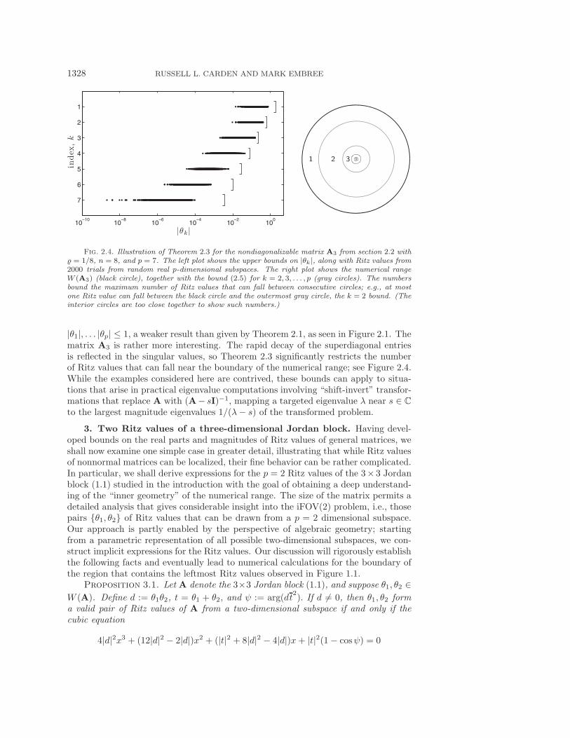
Fig. 2.4. Illustration of Theorem 2.3 for the nondiagonalizable matrix A3 from section 2.2 with� = 1/8, n = 8, and p = 7. The left plot shows the upper bounds on |θk|, along with Ritz values from2000 trials from random real p-dimensional subspaces. The right plot shows the numerical rangeW (A3) (black circle), together with the bound (2.5) for k = 2, 3, . . . , p (gray circles). The numbersbound the maximum number of Ritz values that can fall between consecutive circles; e.g., at mostone Ritz value can fall between the black circle and the outermost gray circle, the k = 2 bound. (Theinterior circles are too close together to show such numbers.)

|θ1|, . . . |θp| ≤ 1, a weaker result than given by Theorem 2.1, as seen in Figure 2.1. Thematrix A3 is rather more interesting. The rapid decay of the superdiagonal entriesis reflected in the singular values, so Theorem 2.3 significantly restricts the numberof Ritz values that can fall near the boundary of the numerical range; see Figure 2.4.While the examples considered here are contrived, these bounds can apply to situa-tions that arise in practical eigenvalue computations involving “shift-invert” transfor-mations that replace A with (A− sI)−1, mapping a targeted eigenvalue λ near s ∈ C

to the largest magnitude eigenvalues 1/(λ− s) of the transformed problem.

3. Two Ritz values of a three-dimensional Jordan block. Having devel-oped bounds on the real parts and magnitudes of Ritz values of general matrices, weshall now examine one simple case in greater detail, illustrating that while Ritz valuesof nonnormal matrices can be localized, their fine behavior can be rather complicated.In particular, we shall derive expressions for the p = 2 Ritz values of the 3× 3 Jordanblock (1.1) studied in the introduction with the goal of obtaining a deep understand-ing of the “inner geometry” of the numerical range. The size of the matrix permits adetailed analysis that gives considerable insight into the iFOV(2) problem, i.e., thosepairs {θ1, θ2} of Ritz values that can be drawn from a p = 2 dimensional subspace.Our approach is partly enabled by the perspective of algebraic geometry; startingfrom a parametric representation of all possible two-dimensional subspaces, we con-struct implicit expressions for the Ritz values. Our discussion will rigorously establishthe following facts and eventually lead to numerical calculations for the boundary ofthe region that contains the leftmost Ritz values observed in Figure 1.1.

Proposition 3.1. Let A denote the 3×3 Jordan block (1.1), and suppose θ1, θ2 ∈W (A). Define d := θ1θ2, t = θ1 + θ2, and ψ := arg(dt

2). If d �= 0, then θ1, θ2 form

a valid pair of Ritz values of A from a two-dimensional subspace if and only if thecubic equation

4|d|2x3 + (12|d|2 − 2|d|)x2 + (|t|2 + 8|d|2 − 4|d|)x+ |t|2(1− cosψ) = 0


has a root x ∈ [0, (|d|+ 1/|d|)/2− 1]. If d = 0, then θ1 and θ2 form a valid Ritz pairif and only if |t| ≤ 1/2.

In particular, for any θ1 ∈W (A), θ2 = −θ1 is a valid Ritz value.This detailed understanding requires an expression for the Ritz values for all

possible two-dimensional subspaces. Since p = n − 1 = 2, the parameterization ofall subspaces is simplified by the fact that every (n− 1)-dimensional subspace of Cn,represented by V ∈ Cn×(n−1), V∗V = I, can be characterized by any nonzero vectorv orthogonal to the subspace, V∗v = 0. This v, which we shall always take to be aunit vector, uniquely determines the range of V. Any orthonormal basis for Ran(V)gives the same Ritz values. We use these facts via the matrix adjugate, as donefor normal matrices in [5]. The adjugate (or classical adjoint) [9, p. 21] of a matrixsatisfies

[adj(A)]ij = (−1)i+j det((A)ji

)= (detA)[A−1]ij ,

where [·]ij refers to the (i, j) element of a matrix, and (·)ji is the matrix formedby deleting row j and column i from a matrix. The second equality holds only forinvertible A. For unitary U, the adjugate satisfies adj(U∗AU) = U∗adj(A)U. Thematrix U = [Vv] ∈ Cn×n is unitary, so

det(V∗AV) = det((U∗AU)nn) = [adj(U∗AU)]nn = [U∗adj(A)U]nn = v∗adj(A)v.

Similarly, det(λI−V∗AV), the characteristic polynomial of the restriction of a matrixA to the subspace orthogonal to v, can be determined by computing the Rayleighquotient of adj(λI−A) with v.

When A is an n× n Jordan block,

adj(λI−A) =

n−1∑j=0

λn−1−jAj ,

so the coefficient of λj in the characteristic polynomial det(λI − V∗AV) is simplycj = v∗An−1−jv. These coefficients are symmetric polynomials in the eigenvalues ofV∗AV. For n = 3,

v∗Av = −(θ1 + θ2) = −tr(V∗AV),(3.1)

v∗A2v = θ1θ2 = det(V∗AV),(3.2)

where θ1 and θ2 are the eigenvalues of V∗AV. Without loss of generality (since eiφvgenerates the same Ritz values for any φ), write the unit vector v as

v =

⎡⎣ cosφ1− sinφ1 cosφ2 e

iφ3

sinφ1 sinφ2 eiφ4

⎤⎦(3.3)

for independent real parameters φ1, φ2, φ3, φ4 ∈ [0, 2π), thus giving

θ1 + θ2 = cosφ1 sinφ1 cosφ2 eiφ3 + sin2 φ1 cosφ2 sinφ2 e

i(φ4−φ3),(3.4)

θ1θ2 = cosφ1 sinφ1 sinφ2 eiφ4 .(3.5)

The Ritz values are completely determined by these two formulas. Hence, for there tobe a two-dimensional subspace V that gives both θ1 and θ2 as Ritz values, there must


exist real φ1, . . . , φ4 that satisfy (3.4)–(3.5). Without loss of generality, let arg θ1θ2 =φ4. (If arg(θ1θ2) �= φ4, one can modify φ3 and either φ1 or φ2: set φ4 → arg θ1θ2,φ3 → φ3 + π, and either φ1 → π − φ1 or φ2 → φ2 + π.) Given this parametricrepresentation of the possible Ritz values, we seek implicit expressions relating θ1and θ2. From these expressions, we will find the number of distinct subspaces thatgenerate a given pair of Ritz value combinations and, where possible, give formulasfor v in terms of θ1 and θ2.

3.1. A Ritz value at zero. We wish to use (3.5) to eliminate φ4 from (3.4). Toperform this elimination, cosφ1 sinφ1 sinφ2 must be nonzero. First we address thespecial case where cosφ1 sinφ1 sinφ2 = 0, which implies by (3.5) that at least one ofthe Ritz values is zero; say, θ1 = 0. Three scenarios are possible from (3.4):

• sinφ1 = 0, in which case θ2 = 0;• cosφ1 = 0, in which case θ2 = cosφ2 sinφ2 e

i(φ4−φ3), allowing θ2 to take anyvalue in the disk {z ∈ C : |z| ≤ 1/2};

• sinφ2 = 0, in which case θ2 = ± cosφ1 sinφ1 eiφ3 , allowing θ2 to take any

value in the disk {z ∈ C : |z| ≤ 1/2}.Hence, any pair of Ritz values {0, θ} is possible for |θ| ≤ 1/2: θ = 0 only correspondsto the subspaces defined by v ∈ {e1, e2, e3}, the set of canonical basis vectors; each0 < |θ| < 1/2 corresponds to the four subspaces orthogonal to one of the vectors

v =

⎡⎢⎢⎢⎢⎣0

−√

1±√

1−4|θ|22

θ|θ|

√1∓

√1−4|θ|22

⎤⎥⎥⎥⎥⎦ , v =

⎡⎢⎢⎢⎢⎣−√

1∓√

1−4|θ|22

θ|θ|

√1±

√1−4|θ|22

0

⎤⎥⎥⎥⎥⎦ .

For these v, the subspace Ran(V) = v⊥ must contain either a left or a right eigen-vector of A. For |θ| = 1/2 there are only two choices of v.2 Already, we see that ifone Ritz value is at zero, the other cannot be near the boundary of W (A), i.e., in theregion {z ∈ C : 1/2 < |z| ≤ √

2/2}. This set is shown, along with similar regions forfixed nonzero Ritz values, in Figure 3.2 at the end of this section.

3.2. Zero trace. Having handled all θ1θ2 = 0 cases, now assume θ1θ2 �= 0.Using (3.5), substitute

eiφ4 =θ1θ2

cosφ1 sinφ1 sinφ2(3.6)

into (3.4) to eliminate φ4:

(cos2 φ1 sinφ1eiφ3 + θ1θ2 sinφ1e

−iφ3) cosφ2 = (θ1 + θ2) cosφ1.(3.7)

If the expression on the left is zero, so too must be the expression on the right. Thusθ1 + θ2 = 0, since cosφ1 = 0 gives θ1θ2 = 0, handled above. If the coefficient ofcosφ2 on the left of (3.7) is zero, then θ21 = cos2 φ1e

2iφ3 ; if cosφ2 = 0, then −θ21 =cosφ1 sinφ1e

iφ4 . Together, these cases give four possible solutions, corresponding to

2For this nonnormal A, the entries of v are uniquely determined by functions that involvesquare roots of the Ritz values; in contrast, for normal matrices the analogous formulas only involvepolynomial expressions of θ1 and θ2 [5].


the vectors

v =

⎡⎢⎣ θ1

±√1− 2|θ1|2−θ1

⎤⎥⎦ , v =

⎡⎢⎢⎢⎣θ1|θ1|

√1∓

√1−4|θ1|42

0

− θ1|θ1|

√1±

√1−4|θ1|42

⎤⎥⎥⎥⎦ .(3.8)

For θ1 =√2/2 on the boundary ofW (A), there is one vector: v = [

√2/2, 0,−√

2/2]T.These calculations imply that any pair θ1, θ2 ∈ W (A) satisfying θ1 = −θ2 is a

valid Ritz pair from some two-dimensional subspace.

3.3. Some conjugate pairs. Continuing with a nonzero determinant, θ1θ2 �= 0,we can now assume the coefficient of cosφ2 on the left of (3.7) is nonzero. Thenfrom (3.7),

cosφ2 =(θ1 + θ2) cosφ1

(cos2 φ1 eiφ3 + θ1θ2 e−iφ3) sinφ1,

thus determining φ2 in terms of φ1, φ3, and the Ritz values.To simplify the coefficients, write d := θ1θ2 and t := θ1 + θ2 for the determinant

and trace of V∗AV, so

cosφ2 =t cosφ1

(cos2 φ1 eiφ3 + de−iφ3) sinφ1.(3.9)

Requiring the imaginary part of (3.9) to be zero yields

(Im(t) cos2 φ1 − Im(dt)) cosφ3 = (Re(t) cos2 φ1 − Re(dt)) sinφ3,(3.10)

and so

tanφ3 =Im(t) cos2 φ1 − Im(dt)

Re(t) cos2 φ1 − Re(dt).

Hence φ3 is ill-defined when the coefficients of cosφ3 and sinφ3 in (3.10) are bothzero, i.e., when t cos2 φ1 = dt. In this subsection we analyze this special situation,then return to the general case in section 3.4.

The expression t cos2 φ1 = dt is invariant to rotations of the Ritz values aboutthe origin in the complex plane, since a rotation of both Ritz values by the angle γcorresponds to multiplying the determinant by e2iγ and the trace by eiγ :

(teiγ) cos2 φ1 = (de2iγ)teiγ .(3.11)

Hence we can assume that the trace is real and positive, and since t cos2 φ1 = dt, thedeterminant is also real and positive.

With d = cos2 φ1 and t > 0, we can use φ4 = 0 and (3.5) to conclude cos2 φ2 =(2d− 1)/(d− 1). Substituting this expression into (3.9) gives

8d2 − 4d+ t2 sec2 φ3 = 0.(3.12)

One can show that the only real Ritz values consistent with (3.12) are θ1 = θ2 = 0,a case covered earlier. Hence the Ritz values considered here must form complex


conjugate pairs. Letting θ = x+ iy, we have d = x2 + y2 and t = 2x, so (3.12) implies

0 = 2(x2 + y2)2 − (x2 + y2) + x2 sec2 φ3

≥ 2(x2 + y2)2 − (x2 + y2) + x2

= 2

((x2 − 1

8

)+

(y −

√2

4

)2)((

x2 − 1

8

)+

(y +

√2

4

)2)

= 2

(∣∣∣∣θ − i

√2

4

∣∣∣∣2 − 1

8

)(∣∣∣∣θ + i

√2

4

∣∣∣∣2 − 1

8

).

This last expression is nonpositive for all θ in the union of the closed disks of radius√2/4 centered at ±i√2/4 in the complex plane: all the Ritz values for this scenario

(d �= 0, t > 0, d = cos2 φ1) come in complex conjugate pairs and lie in these disks.Ritz values corresponding to d �= 0, t �= 0, and t cos2 φ1 = dt correspond to two

possible values for v in the form (3.3):

v =

⎡⎢⎢⎣√d

− |t|2√

|d| ± i√1− 2|d| − |t|2

4|d|√d

⎤⎥⎥⎦ ,(3.13)

where√d is chosen such that arg(

√d) = arg(t). If t = 0, this expression essentially

reduces to the first vector in (3.8). In the special case of 1−2|d|− |t|2/4|d| = 0, (3.13)gives just one vector, generating Ritz values that lie on the boundary of the disksmentioned above (suitably rotated by eiγ).

3.4. General case. Return now to (3.9). Having analyzed t cos2 φ1 = dt, wecan address the general case, where t cos2 φ1 �= dt. Equation (3.10), together with therequirement that eiφ3 must have unit modulus, gives

eiφ3 =t cos2 φ1 − dt∣∣t cos2 φ1 − dt

∣∣ .(3.14)

The expressions for φ2, φ3, and φ4 in (3.9), (3.14), and (3.6) provide an expressionfor v in terms of d, t, and cosφ1:

v =

⎡⎢⎢⎢⎢⎢⎣cosφ1

−cosφ1(t cos2 φ1 − dt)

cos4 φ1 − |d|2d

cosφ1

⎤⎥⎥⎥⎥⎥⎦ .(3.15)

The second entry has a pole at cos2 φ1 = |d|; the residue at this pole is zero if and only

if arg(dt2) = 0, which corresponds to Ritz values that are equivalent to a complex

conjugate pair, as handled in the last subsection. For this vector to have norm one,cosφ1 must satisfy

0 = (cos12 φ1 + |d|6)− (cos10 φ1 + |d|4 cos2 φ1)+ (|t|2 − |d|2)(cos8 φ1 + |d|2 cos4 φ1) + (2|d|2 − dt

2 − dt2) cos6 φ1.(3.16)

The right-hand side is a polynomial in cosφ1 that involves only even powers, consistentwith ±v generating the same subspace Ran(V). The terms are arranged to emphasize


that the polynomial is |d|2-self-reciprocal, i.e., if cos2 φ1 is a solution, then |d|2/cos2 φ1is also a solution: a consequence of A being similar to its transpose via a permuta-tion. Using the |d|2-self-reciprocal property, make the substitution cos2 φ1 → |d|ey toreduce (3.16) to

0 = 4|d|2 cosh3 y − 2|d| cosh2 y + (−4|d|2 + |t|2) cosh y − |t|2 cosψ + 2|d|,(3.17)

where ψ := arg(dt2). This equation is cubic in cosh y, so one can write out the solution

exactly in terms of d, t, and cosψ; however, the complexity of the expressions limitsthe amount of insight that can be gained. Numerical calculations indicate that atmost two of the solutions to this equation correspond to actual Ritz value pairs. Thiswould imply that the generic case gives at most four distinct subspaces that generatethe same pair of Ritz values.

3.5. Solving iFOV(2). Having carefully studied the relationship between theRitz values and their generating subspaces, we return to our main motivation, theiFOV(2) problem for the Jordan block: given two candidate Ritz values θ1, θ2 ∈W (A), determine if there exists some two-dimensional subspace such that θ1 andθ2 are simultaneously Ritz values of A. The general analysis of the last subsectionenables an easy test for solutions to iFOV(2).

Given θ1 and θ2, form ψ := arg(dt2) and let δ := |d| and τ := |t|. Since cosh(y) ≥ 1

for real y, define x := cosh(y)− 1. Now expand (3.17) as a cubic polynomial in x:

4δ2x3 + (12δ2 − 2δ)x2 + (τ2 + 8δ2 − 4δ)x+ τ2(1− cosψ) = 0.(3.18)

We want to show that all roots x that correspond to solutions of iFOV(2) must bein the interval [0, (δ + 1/δ)/2 − 1]. As cos2 φ1 = δey and 0 ≤ cos2 φ1 ≤ 1, we haveey ∈ [0, 1/δ]; the δ2-self-reciprocal property of (3.16) ensures that δ2/ cos2 φ1 = δe−y

is also a root, and so we must also have e−y ∈ [0, 1/δ]. These requirements togethergive e±y ∈ [δ, 1/δ], so cosh y ∈ [1, (δ + 1/δ)/2], i.e., all valid roots x must be in theinterval [0, (δ + 1/δ)/2− 1]. This gives a quick way to check if iFOV(2) is solvable.

• Given θ1, θ2 ∈W (A), form ψ := arg(dt2), δ := |θ1θ2|, and τ := |θ1 + θ2|.

• Compute the roots of the cubic equation (3.18).• If at least one root x ∈ [0, (δ+1/δ)/2− 1], then iFOV(2) has a valid solution.

This test enables one to check the solvability of iFOV(2) numerically for a candi-date pair of Ritz values. However, considerable additional structure about the (δ, τ)pairs for which iFOV(2) is solvable can be discovered if one is willing to dig deeperinto (3.18). Descartes’ rule of signs (see, e.g., [18, p. 319]) characterizes when (3.18)can have real positive roots by counting the sign changes in the ordered nonzero(real-valued) coefficients. The first coefficient 4δ2 is positive for δ > 0. The secondcoefficient 12δ2 − 2δ is negative for δ ∈ (0, 1/6) and positive for δ > 1/6. The thirdcoefficient τ2 + 8δ2 − 4δ is negative in the interior of an ellipse in the (δ, τ) planecentered at (1/4, 0) with semimajor and semiminor axes of length

√2/2 and 1/4 and

positive on the exterior of this ellipse. The last coefficient is always nonnegative, be-ing zero when cosψ = 1. We subdivide the relevant part of the (δ, τ) plane into fourregions depending on the signs of the middle two coefficients; see Figure 3.1.

12δ2 − 2δ τ2 + 8δ2 − 4δ # sign changes # positive rootsI − − 2 0 or 2II − + 2 0 or 2III + − 2 0 or 2IV + + 0 0


0 1/6 1/20

1/2

2/3

√2/2

IV

IIII

II

δ

τ

0 1/6 1/20

1/2

2/3

√2/2

δ

τ

A: all ψ valid

B: some ψ valid

C: no ψ valid

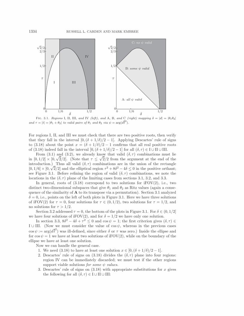
Fig. 3.1. Regions I, II, III, and IV (left), and A, B, and C (right) mapping δ = |d| = |θ1θ2|and τ = |t| = |θ1 + θ2| to valid pairs of θ1 and θ2 via ψ = arg(dt

2).

For regions I, II, and III we must check that there are two positive roots, then verifythat they fall in the interval [0, (δ + 1/δ)/2 − 1]. Applying Descartes’ rule of signsto (3.18) about the point x = (δ + 1/δ)/2 − 1 confirms that all real positive rootsof (3.18) indeed fall in the interval [0, (δ + 1/δ)/2− 1] for all (δ, τ) ∈ I ∪ II ∪ III.

From (3.1) and (3.2), we already know that valid (δ, τ) combinations must liein [0, 1/2] × [0,

√2/2]. (Note that τ ≤ √

2/2 from the argument at the end of theintroduction.) Thus all valid (δ, τ) combinations are in the union of the rectangle[0, 1/6]× [0,

√2/2] and the elliptical region τ2 + 8δ2 − 4δ ≤ 0 in the positive orthant;

see Figure 3.1. Before refining the region of valid (δ, τ) combinations, we note thelocations in the (δ, τ) plane of the limiting cases from sections 3.1, 3.2, and 3.3.

In general, roots of (3.18) correspond to two solutions for iFOV(2), i.e., twodistinct two-dimensional subspaces that give θ1 and θ2 as Ritz values (again a conse-quence of the similarity of A to its transpose via a permutation). Section 3.1 analyzedδ = 0, i.e., points on the left of both plots in Figure 3.1. Here we have three solutionsof iFOV(2) for τ = 0, four solutions for τ ∈ (0, 1/2), two solutions for τ = 1/2, andno solutions for τ > 1/2.

Section 3.2 addressed τ = 0, the bottom of the plots in Figure 3.1. For δ ∈ (0, 1/2]we have four solutions of iFOV(2), and for δ = 1/2 we have only one solution.

In section 3.3, 8δ2 − 4δ + τ2 ≤ 0 and cosψ = 1; the first criterion gives (δ, τ) ∈I ∪ III. (Now we must consider the value of cosψ, whereas in the previous cases

cosψ := arg(dt2) was ill-defined, since either δ or τ was zero.) Inside the ellipse and

for cosψ = 1 we have at least two solutions of iFOV(2), while on the boundary of theellipse we have at least one solution.

Now we can handle the general case.1. We need (3.18) to have at least one solution x ∈ [0, (δ + 1/δ)/2− 1].2. Descartes’ rule of signs on (3.18) divides the (δ, τ) plane into four regions:

region IV can be immediately discarded; we must test if the other regionssupport viable solutions for some ψ values.

3. Descartes’ rule of signs on (3.18) with appropriate substitutions for x givesthe following for all (δ, τ) ∈ I ∪ II ∪ III:


(a) (3.18) always has exactly one negative root;(b) all nonnegative roots of (3.18) fall in the interval [0, (δ + 1/δ)/2− 1].

4. Consider the discriminant [11] of the cubic (3.18) with real-valued coefficients:

4δ2(16δ2 − 128δ4 + 256δ6 − 80δ2τ2 − 192δ4τ2 + τ4 + 48δ2τ4(3.19)

−4τ6 − 8δτ2 cosψ + 288δ3τ2 cosψ + 36δτ4 cosψ − 108δ2τ4 cos2 ψ).

(a) If this discriminant is negative, then (3.18) has one real root: Descartes’rule of signs already showed there must be either zero or two positiveroots, so in this case (3.18) has no positive roots.

(b) If the discriminant is zero, all roots are real, with one of them a doubleroot. Given the above observations, this double root must be nonnegative.

(c) If the discriminant is positive, all roots are real and distinct, so theremust be two nonnegative solutions.

5. Now ascertain the sign of the discriminant, seeking regions where we canmake a definitive statement about the solvability of iFOV(2) for all ψ or forsome subset of ψ.(a) The discriminant is quadratic in cosψ, with negative leading coefficient;

hence it opens down. If it has real roots, then for all cosψ values betweenthe roots, the discriminant is positive. With the aid of rather technicalsymbolic calculations, we can identify three regions of the (δ, τ) plane,illustrated in the right plot in Figure 3.1:A: For 0 < δ < 1/2 and 0 < τ < 1/2− δ, the Ritz value pair exists for

all cosψ ∈ [−1, 1]; hence any value of ψ := arg(dt2) is valid.

B: For 0 < δ < 1/6 and 1/2− δ < τ < 1/2 + δ, or 1/6 < δ < 1/2 and1/2 − δ < τ <

√4δ − 8δ2, the Ritz value pair exists only for some

cosψ ∈ [−1, 1]; some values of cosψ ∈ [−1, 1] do not correspond tovalid Ritz value pairs.

C: For all other values of δ and τ , no choice of cosψ ∈ [−1, 1] will yieldsolutions; such δ and τ never correspond to valid Ritz value pairs.

In summary, if θ1 and θ2 correspond to δ = |θ1θ2| and τ = |θ1 + θ2| that fall inregion A, iFOV(2) is solvable; in region B, iFOV(2) might be solvable, depending on

ψ = arg(θ1θ2(θ1 + θ2)2); in region C, iFOV(2) is not solvable.

3.6. Restricting leftmost Ritz values. Given θ1, the results of the previoussections do not immediately reveal where θ2 can be located; however, they do suggesta recipe for determining such regions. Without loss of generality we may assume thatθ1 is real and nonnegative. From the definition of trace and determinant, the followingequations relate τ , δ, and cosψ to θ1 and θ2:

δ2 = θ21((Re θ2)

2 + (Im θ2)2),(3.20a)

τ2 = (θ1 +Re θ2)2 + (Im θ2)

2,(3.20b)

cosψ =θ1Re(θ2(θ1 + θ2)

2)

δτ2.(3.20c)

For fixed θ1 ≥ 0 and Re θ2 we can see that as Im θ2 increases, so do δ and τ . From


Fig. 3.2. For A equal to the three-dimensional Jordan block, the outermost circle shows theboundary of W (A). For three fixed choices of θ1 (•), the gray regions show where θ2 can fall.

these equations we can determine a hyperbola in the (δ, τ) plane,

τ2 − δ2/θ21 = θ21 + 2θ1Re θ2.(3.21)

The hyperbola opens up for Re θ2 > −θ1/2 and to the right otherwise. For this fixedθ1 and Re θ2, we seek all Im θ2 values for which θ1 and θ2 can simultaneously be Ritzvalues. For a point (δ, τ) on the hyperbola (3.21) to correspond to a valid Ritz pair, wemust be able to find a real value for Im θ2 from the given θ1 and Re θ2 via the equationsδ = |θ1θ2| and τ = |θ1+θ2|. The leftmost point in the first quadrant of the (δ, τ) planealong the hyperbola (3.21) that gives a real value for Im θ2 occurs when Im θ2 = 0,i.e., (δ, τ) = (θ1|Re θ2|, |θ1+Re θ2|). The range of Im θ2 for which iFOV(2) is solvablecorresponds to when the curve (3.20) is inside the region of feasible (δ, τ, cosψ). Fromsymmetry, we know that the set of permissible Im θ2 is symmetric about the real axis.We have numerically observed that this set does not have any gaps, i.e., if iFOV(2)is solvable for given θ1 ≥ 0 and Re θ2, then Im θ2 can lie anywhere in some interval[−α, α]. In Figure 3.2, we show the regions where θ2 must lie in order for iFOV(2) tobe solvable for three different values of θ1.

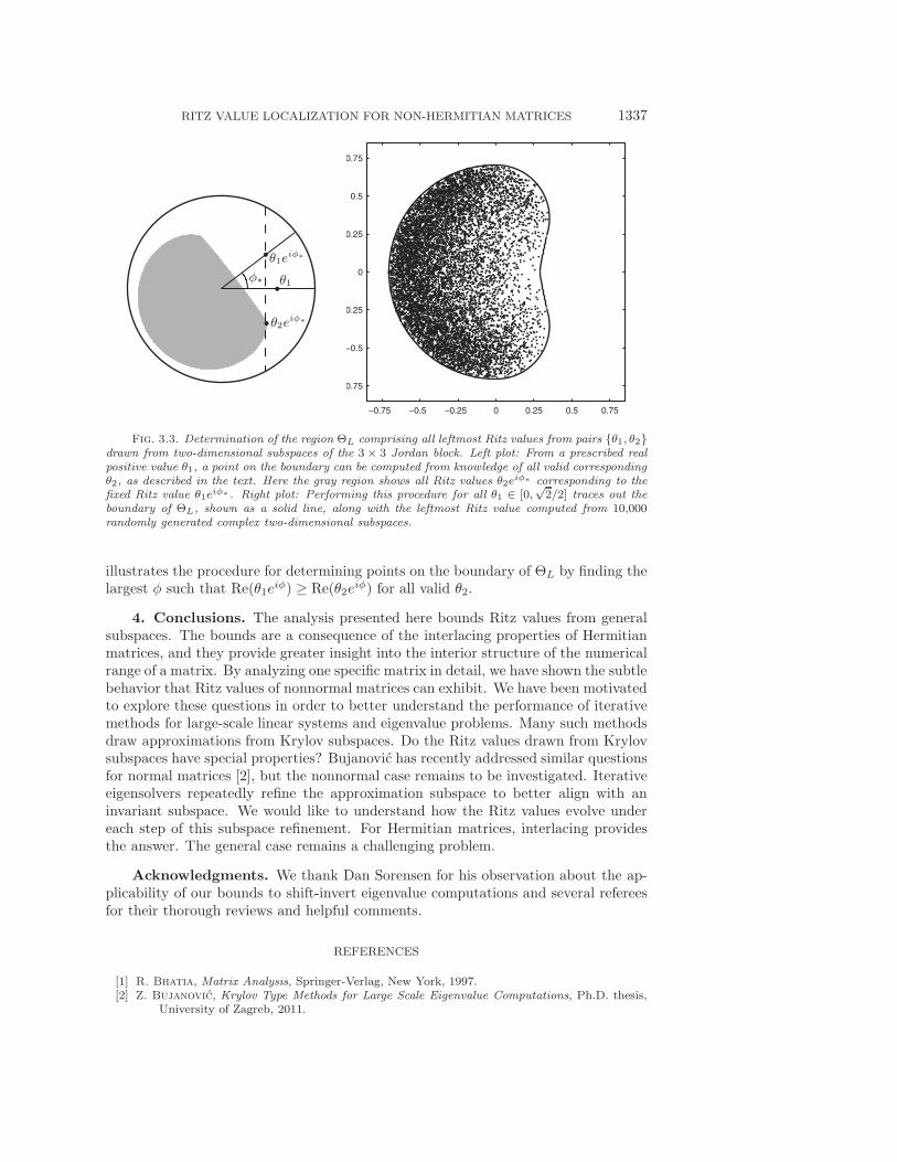
Finally, we return to the plot that began this investigation, Figure 1.1. Can wecalculate a sharp boundary for the region that contains the leftmost Ritz value?

Let ΘL denote the set of all leftmost Ritz values from two-dimensional subspaces,i.e., the set of all θ1 ∈ W (A) such that there exists some valid corresponding Ritzvalue θ2 with Re(θ1) ≤ Re(θ2).

We wish to characterize the boundary of ΘL. From the majorization boundsin section 2, the real part of any point on the boundary of ΘL must be less thanor equal to

√2/4; this gives the bound in Figure 1.1. We claim that for any real,

positive θ1, if θ1 > Re θ2 for all valid θ2, then there exists a unique φ∗ ∈ [0, π/2]such that Re(θ1e

iφ∗) ≥ Re(θ2eiφ∗) for all valid θ2, with equality for at least one

θ2; see the left plot in Figure 3.3. First, such a φ∗ must be less than or equal toπ/2, since there always exists a restriction such that θ2 = −θ1 (as in section 3.2).Second, equality must be attained for some θ2, as the set of θ2 for a given θ1 isdetermined by the intersection of two closed sets in (δ, τ, cosψ) space, and by theprevious remark we know this intersection is not empty. Last, the uniqueness of φ∗follows from the attainment of equality in Re(θ1e

iφ∗) ≥ Re(θ2eiφ∗) for some θ2, since

for any φ ∈ (φ∗, π/2] there must exist at least one θ2 such that Re(θ1eiφ) ≤ Re(θ2e

iφ).Thus θ1e

iφ∗ must be on the boundary separating ΘL from ΘL \W (A), as we alsohave Re(θ1e

iφ) > Re(θ2eiφ) for φ ∈ [0, φ∗) and for all valid θ2. (If {θ1, θ2} is a valid

Ritz pair, so too is {θ1eiφ, θ2eiφ}.) The boundaries of W (A) and ΘL coincide in theleft half-plane, which follows from the same argument with θ1 =

√2/2. Figure 3.3


−0.75 −0.5 −0.25 0 0.25 0.5 0.75

0.75

−0.5

0.25

0

0.25

0.5

0.75

θ1eiφ∗

θ2eiφ∗

φ∗ θ1

Fig. 3.3. Determination of the region ΘL comprising all leftmost Ritz values from pairs {θ1, θ2}drawn from two-dimensional subspaces of the 3 × 3 Jordan block. Left plot: From a prescribed realpositive value θ1, a point on the boundary can be computed from knowledge of all valid correspondingθ2, as described in the text. Here the gray region shows all Ritz values θ2eiφ∗ corresponding to thefixed Ritz value θ1eiφ∗ . Right plot: Performing this procedure for all θ1 ∈ [0,

√2/2] traces out the

boundary of ΘL, shown as a solid line, along with the leftmost Ritz value computed from 10,000randomly generated complex two-dimensional subspaces.

illustrates the procedure for determining points on the boundary of ΘL by finding thelargest φ such that Re(θ1e

iφ) ≥ Re(θ2eiφ) for all valid θ2.

4. Conclusions. The analysis presented here bounds Ritz values from generalsubspaces. The bounds are a consequence of the interlacing properties of Hermitianmatrices, and they provide greater insight into the interior structure of the numericalrange of a matrix. By analyzing one specific matrix in detail, we have shown the subtlebehavior that Ritz values of nonnormal matrices can exhibit. We have been motivatedto explore these questions in order to better understand the performance of iterativemethods for large-scale linear systems and eigenvalue problems. Many such methodsdraw approximations from Krylov subspaces. Do the Ritz values drawn from Krylovsubspaces have special properties? Bujanovic has recently addressed similar questionsfor normal matrices [2], but the nonnormal case remains to be investigated. Iterativeeigensolvers repeatedly refine the approximation subspace to better align with aninvariant subspace. We would like to understand how the Ritz values evolve undereach step of this subspace refinement. For Hermitian matrices, interlacing providesthe answer. The general case remains a challenging problem.

Acknowledgments. We thank Dan Sorensen for his observation about the ap-plicability of our bounds to shift-invert eigenvalue computations and several refereesfor their thorough reviews and helpful comments.

REFERENCES

[1] R. Bhatia, Matrix Analysis, Springer-Verlag, New York, 1997.[2] Z. Bujanovic, Krylov Type Methods for Large Scale Eigenvalue Computations, Ph.D. thesis,

University of Zagreb, 2011.


[3] R. Carden, A simple algorithm for the inverse field of values problem, Inverse Problems, 25(2009), 115019.

[4] R. Carden, Ritz Values and Arnoldi Convergence for Non-Hermitian Matrices, Ph.D. thesis,Rice University, 2011.

[5] R. Carden and D. Hansen, Ritz Values of Normal Matrices and Ceva’s Theorem, Technicalreport TR 11-16, Department of Computational and Applied Mathematics, Rice University,2011.

[6] C. Chorianopoulos, P. Psarrakos, and F. Uhlig, A method for the inverse numerical rangeproblem, Electron. J. Linear Algebra, 20 (2010), pp. 198–206.

[7] M. Embree, The Arnoldi eigenvalue iteration with exact shifts can fail, SIAM J. Matrix Anal.Appl., 31 (2009), pp. 1–10.

[8] K. E. Gustafson and D. K. M. Rao, Numerical Range: The Field of Values of LinearOperators and Matrices, Springer-Verlag, New York, 1997.

[9] R. A. Horn and C. R. Johnson, Matrix Analysis, Cambridge University Press, Cambridge,UK, 1985.

[10] R. A. Horn and C. R. Johnson, Topics in Matrix Analysis, Cambridge University Press,Cambridge, UK, 1991.

[11] R. S. Irving, Integers, Polynomials, and Rings: A Course in Algebra, Springer–Verlag, NewYork, 2004.

[12] R. B. Lehoucq, D. C. Sorensen, and C. Yang, ARPACK Users’ Guide: Solution of Large-Scale Eigenvalue Problems with Implicitly Restarted Arnoldi Methods, SIAM, Philadelphia,1998.

[13] S. M. Malamud, Inverse spectral problem for normal matrices and the Gauss–Lucas theorem,Trans. Amer. Math. Soc., 357 (2004), pp. 4043–4064.

[14] A. W. Marshall, I. Olkin, and B. C. Arnold, Inequalities: Theory of Majorization and ItsApplications, 2nd ed., Springer, New York, 2011.

[15] B. N. Parlett, The Symmetric Eigenvalue Problem, SIAM, Philadelphia, 1998.[16] P. J. Psarrakos and M. J. Tsatsomeros, An envelope for the spectrum of a matrix, Cen.

Eur. J. Math., 10 (2012), pp. 292–302.[17] J. F. Queiro and A. L. Duarte, On the Cartesian decomposition of a matrix, Linear Multi-

linear Algebra, 18 (1985), pp. 77–85.[18] Q. I. Rahman and G. Schmeisser, Analytic Theory of Polynomials, Oxford University Press,

Oxford, UK, 2002.[19] D. C. Sorensen, Implicit application of polynomial filters in a k-step Arnoldi method, SIAM

J. Matrix Anal. Appl., 13 (1992), pp. 357–385.[20] F. Uhlig, An inverse field of values problem, Inverse Problems, 24 (2008), 055019.

Documents

Ritz values - Computational and Applied Mathematicsembree/87269.pdf · SIAM J. MATRIX ANAL. APPL. c 2012 Society for Industrial and Applied Mathematics Vol. 33, No. 4, pp. 1320–1338