River Analysis and Climate Change: Continuous Prediction of Clay-Bed Erosion in Watts Creek

Colin Brennan

A thesis submitted in partial fulfillment of the requirements for the degree of

Master of Applied Science in Civil Engineering

The Ottawa-Carleton Institute for Civil Engineering Department of Civil Engineering

Faculty of Engineering University of Ottawa

© Colin Brennan, Ottawa, Canada, 2017

ii  

Acknowledgements

First I would like to thank Dr. Ioan Nistor, it was during his course on fluid mechanics a decade

ago that I was introduced to the technical challenges and elegance of studying flowing water,

I’ve been intrigued ever since.

Thank you to my supervisors Dr. Colin Rennie and Dr. Ousmane Seidou, your encouragement,

guidance and suggestions for improvement have allowed me to be successful during this chapter

of my academic life. Your dedication to your fields of research and to supporting your students

and sharing your knowledge has produced a group of students with passion for their work and a

respect for collaboration, it was a pleasure to be one of them.

Thank you to my many uOttawa and JFSA colleagues, I’ve been lucky and privileged to work

with all of you. I’ve enjoyed our discussions and benefitted from your suggestions throughout

this project. Thanks in particular to Parna Parsapour-Moghaddam, I have benefitted greatly from

our collaboration together thus far and look forward to working with you on future projects.

J.F. Sabourin, thank you for encouraging me to pursue this degree, providing the flexibility to

make it possible and for your help with programming and hydrology.

Thank you to my Mom and Dad, Gina and Mike Brennan, for encouraging me to attend

university and to pick my own path. There were times throughout this work when I wasn’t sure

how to move forward and complete the project, but you’ve taught me not to panic at times like

that, somehow everything always gets done.

I have had the benefit of a constant partner to share in the moments of excitement and the

stretches of setbacks throughout this adventure, thank you to my wife, Arwen Moore, for

everything. Since I started this degree, a month before our wedding, you’ve been my sounding

board for ideas, concerns and questions. Thank you for your patience, support and confidence.

 

iii  

Abstract

Predicted future precipitation is downscaled and used to drive a hydrologic model to assess

future erosion potential in a semi-alluvial clay-bed watercourse, Watts Creek. The 21 km2

watershed is predominantly urban, with overall impervious cover of 22%, and the remaining land

use split between agricultural and forested areas. Continuous simulations for the open water year,

excluding spring freshet (April 1st to October 31st) were performed using the SWMHYMO

(Stormwater Management Hydrologic Model) lumped hydrologic modelling platform. A shear

stress exceedance and stream power erosion routine was added to the platform to calculate

erosion potential. To account for uncertainty in the collected data, nine different observed

discharge data sets were used to calibrate the model, each leading to a distinct set of calibrated

parameter values. The difference between the observed data sets lies in the choice of rating

curves and the collection period. The 2041-2080 precipitation outputs of the fourth version of the

Canadian Regional Climate Model (CanRCM4) ran under Representative Concentration

Pathways (RCPs) 4.5 and 8.5 at the MacDonald Cartier International Airport were downscaled

using quantile matching and then used as input to the hydrologic model. For each set of

calibrated parameters, a cumulative effective work index (CWI) based on the reach-averaged

shear stress was calculated for Watts Creek during the open water year using both the historic

(1968 - 2007) and projected future (2041-2080) flows, using a bed material critical shear stress

for entrainment of 3.7 Pa. Results suggest an increase of 75% (resp. 139%) under RCP4.5

(resp. RCP8.5) in CWI compared to historic conditions for the average measured bed strength.

The work index increase is driven by an increased occurrence of above-threshold events, and

more importantly by the increased frequency of large events. The predicted flow regime under

climate change would significantly alter the erosion potential and stability of Watts Creek. A

channel adjustment sensitivity analysis, which balances future erosion potential with historic

potential, was implemented and indicated that the channel could widen in the future from the

current bankfull width of 6.1 m to 8.2 m for RCP4.5 and 10.2 m for RCP8.5. Specific

morphological behaviour should be investigated in more detail, particularly to assess if the

governing erosion mechanism is seasonally dependent, perhaps incising during spring freshet

and widening when the bed is vegetated in the summer.

iv  

Table of Contents

Acknowledgements ......................................................................................................................... ii

Abstract .......................................................................................................................................... iii

List of Figures ................................................................................................................................ vi

List of Tables ................................................................................................................................ vii

List of Symbols ............................................................................................................................ viii

1 Introduction ............................................................................................................................. 1

1.1 Organisation of the Thesis ................................................................................................ 2

1.2 Literature Review ............................................................................................................. 3

1.2.1 River erosion and sediment transport ...................................................................... 3

1.2.2 Climate model output and statistical downscaling ................................................... 5

1.2.3 River erosion under climate change ......................................................................... 8

1.3 Novelty of the Study ...................................................................................................... 10

1.4 Research Objectives ....................................................................................................... 11

1.5 Project Contributors ....................................................................................................... 11

2 Continuous prediction of clay-bed stream erosion in response to climate model output for a small urban watershed................................................................................................................... 12

2.1 Abstract .......................................................................................................................... 12

2.2 Introduction .................................................................................................................... 13

2.3 Materials and Methods ................................................................................................... 14

2.3.1 Study Site ............................................................................................................... 14

2.3.2 Data collection ....................................................................................................... 15

2.3.2.1 Field measurements ............................................................................................... 15

2.3.2.2 Catchment characteristics ...................................................................................... 17

2.3.3 Rating Curve Derivation ........................................................................................ 17

2.3.4 Climate Change Projections ................................................................................... 21

2.3.5 Hydrologic Modelling ............................................................................................ 23

2.3.5.1 Modified Erosion Index Routine ........................................................................... 23

2.3.5.2 Hydrologic Model Setup and Calibration .............................................................. 24

2.4 Results ............................................................................................................................ 28

2.4.1 Model Calibration .................................................................................................. 28

2.4.2 Climate Change Projections ................................................................................... 31

v  

2.4.3 Projected Hydrographs and Erosion ...................................................................... 36

2.5 Discussion ...................................................................................................................... 40

2.6 Conclusions .................................................................................................................... 44

3 Thesis Conclusions ................................................................................................................ 46

3.1 Recommendations for Future Work ............................................................................... 47

References ..................................................................................................................................... 50

Appendix A: Depth, Rain, Flow and Creek profile data collected for Watts Creek ..................... 57

Appendix B: Quantile quantile transform schematic and modelling process flow chart ............. 64 

 

vi  

List of Figures

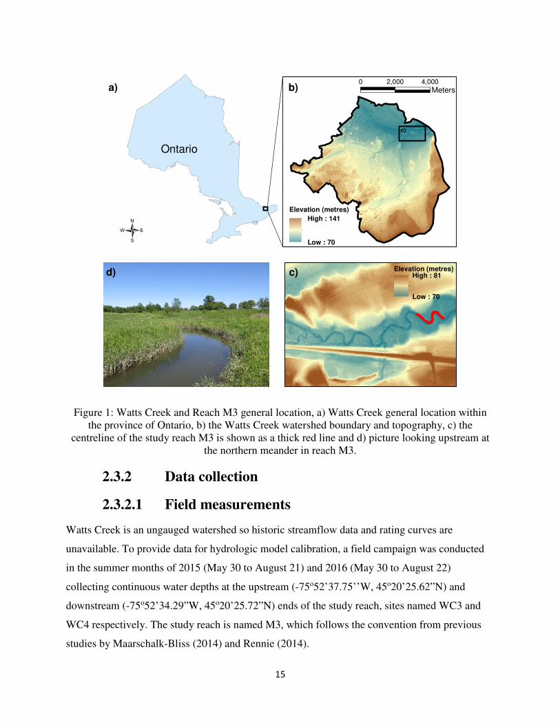
Figure 1: Watts Creek and Reach M3 general location, a) Watts Creek general location within

the province of Ontario, b) the Watts Creek watershed boundary and topography, c)

the centreline of the study reach M3 is shown as a thick red line and d) picture

looking upstream at the northern meander in reach M3. ......................................... 15 

Figure 2: Rating curves for DQ1 (Flow = 1.95*D3.48) and DQ2 for overbank conditions

(Flow = 2.28*D2.52) are shown in (a) and the calculated flow series using the DQ3

relationship for the 2015 and 2016 continuous flow data are shown in (b) ............ 18 

Figure 3: Roughness as a function of depth at the riffle section 40 m downstream of WC4,

part of the DQ3 relationship, the DQ3 power function is n = 0.048*D-1.101 ......... 21 

Figure 4a: Rating Curve DQ1, field and model hydrographs for June 4 to 8 2016 .................. 30 

Figure 4b: Rating Curve DQ2, field and model hydrographs for July 13 to 19 2015 .............. 30 

Figure 4c: Rating Curve DQ3, field and model hydrographs for August 11 to 17 2016 .......... 30 

Figure 5: Monthly Average Rainfall Volume in July, observed and modelled (raw and

corrected i.e. downscaled) during historical period, as well as modelled (raw and

corrected i.e. downscaled) during future period, for calibration (even years) and

validation (odd years), raw data are from CanRCM4 RCP8.5 output. .................... 32 

Figure 6: Erosion potential indicators box and whisker plots for historic and future results.

The range in annual erosion indicators for the open water year (April 1st to October

31st) from each of the 9 model calibrations are shown for four climate datasets. The

climate dataset names are shown on the x-axes: H01) Historic hourly rainfall data

(1968-2007), H02) CanRCM4 QQ corrected data for the historic period (1968-

2007), F45) CanRCM4 RCP4.5 QQ corrected data for the future period (2041-

2080) and F85) CanRCM4 RCP8.5 QQ corrected data for the future period (2041-

2080). ....................................................................................................................... 38 

vii  

List of Tables

Table I: Ranges of Model and Field Maximum Peak flow and total runoff volume from

the 2015 and 2016 calibration periods ................................................................. 28 

Table II: Nash-Sutcliffe model efficiency coefficient for the nine calibration scenarios and

the six applicable validation scenarios ................................................................. 29 

Table III: Open Water Yearly Average Precipitation Indices for Historic and ..........

Future Data ........................................................................................................... 33 

Table IVa: Sensitivity Assessments for Average Open Water Yearly Erosion Indicators:

measured rainfall data and regional climate model with and without bias

correction for the historic period (1968-2007) ..................................................... 34 

Table IVb: Sensitivity Assessments for Average Open Water Yearly Erosion Indicators:

regional climate model results with and without extrapolation by addition for the

future period (2041-2080) .................................................................................... 35 

Table V: Comparison of Future and Historic Average Open Water Yearly Erosion

Potential at Reach M3, Critical Shear Stress of 3.7 Pa ........................................ 36 

 

viii  

List of Symbols

A Flow area (m2)

area Drainage area (km2 or ha)

CN Curve number, infiltration parameter from SCS method

CWI Cumulative work index (Pa*m or J/m2)

DT Time step (minutes)

FOBS Cumulative distribution function (CDF) from the calibration period of the

observed data

FRCM CDF from the calibration period in the raw regional climate model (RCM)

gwresk Rate of baseflow discharge from the groundwater reservoir to surface flow

(mm/day/mm)

Ia Initial abstraction volume (unit depth) for NASHYD commands (mm)

Ia_imp Initial abstraction volume (unit depth) for impervious surfaces (mm)

Ia_per Initial abstraction volume (unit depth) for pervious surfaces (mm)

Ia_recimp Initial abstraction recovery rates for impervious surfaces (hours)

Ia_recper Initial abstraction recovery rates for pervious surfaces (hours)

IET Inter-event time (hours)

InitGWResVol Initial groundwater reservoir volume (mm)

LGI Routing length for impervious surfaces (m)

LGP Routing length for pervious surfaces (m)

mni Manning’s n catchment surface roughness for impervious surfaces

mnp Manning’s n catchment surface roughness for pervious surfaces (sheet flow)

N Nash unit hydrograph number of linear reservoirs

n Manning’s roughness parameter

Rh Hydraulic radius (m)

S Catchment slope (%)

SK Soil storage recovery rate (mm-1)

SLPI Slope for impervious surfaces (%)

SLPP Slope for pervious surfaces (%)

So Channel bed slope (%)

ix  

tp Time to peak (hours)

tc Time of concentration (hours)

τ   Bed shear stress (Pa)

τc   Critical shear stress for entrainment (Pa)

Timp Total imperviousness (%)

v  Main channel velocity (m/s)

VHydCond Vertical hydraulic conductivity (mm/hr)

Ximp Directly connected imperviousness (%)

XCORR Corrected climate variable

XRCM Variable, raw data, extracted from the RCM simulation historic and future

periods

XRCM-CAL Variable, raw data, extracted from the RCM simulation for the calibration

period

γ Specific weight of water (N/m3)

1  

1 Introduction

The City of Ottawa is surrounded by and encompasses a vast array of fresh water resources

including hundreds of creeks and streams (City of Ottawa 2014). Waterways provide lifelines for

citizens and habitat for plants and animals but they also present potential hazards (Knighton

1998) particularly since we seem to be drawn to build too close to riverbanks. Urbanisation has

proceeded with a lack of strategic foresight where on one hand increased impervious cover leads

to increased flood risk and potential bank instability near watercourses (Hammer 1972; FISRWG

1998) and on the other, critical infrastructure is commonly located within floodplains or meander

belts. While the river engineering and planning community have acknowledged this problem for

decades, design and planning to reduce infrastructure risk and protect habitat has largely

proceeded using historic records to define risk and level-of-service (LOS). In a changing climate

and with ongoing environmental degradation, historic precipitation and discharge records may

not be suitable to define risk.

Kundzewicz et al. (2008) summarise the effects of climate change on fresh water resources from

hundreds of papers and assert that this assumption of stationarity in climate for infrastructure

design must be revised in the face of a changing climate. The synthesis report from the fifth

assessment report (AR5) by the Intergovernmental Panel on Climate Change (IPCC) predicts that

increases in precipitation are likely in the region, i.e. Southern Ontario, Canada (IPCC 2014). To

improve resilience of societal infrastructure, we must consider and adapt to possible future

changes in precipitation patterns and their resulting impacts when designing and maintaining

infrastructure.

As a contribution towards this mandate, in this thesis the potential for future erosion of a creek in

Ottawa due to climate change is assessed. The future climate is estimated by downscaling the

predictions of a regional climate model (RCM), future discharge is estimated using a lumped

parameter hydrological model calibrated for the local watershed, and future erosion is estimated

based on predicted bed shear stress.

 

2  

1.1 Organisation of the Thesis

The thesis is comprised of an original research article. The article has been submitted to a peer-

reviewed journal. The article presents a brief review on relevant literature pertaining to the study

of climate model output on riverine erosion. That review is complemented in section 1.2 of this

thesis. Combined, this presents a thorough review of the relevant extant literature. Chapter 1

presents the introduction, thesis organisation, literature review, novelty of the study and lays out

the research aims and contributors to the work.

Chapter 2 presents the article titled Continuous prediction of clay-bed stream erosion in response

to climate model output for a small urban watershed which has been submitted to Hydrological

Processes and is under review at the time of this writing. Field data were collected to measure

the continuous flow time series and hydraulic properties (depth, water surface slope) in Watts

Creek for June, July and August of 2015 and 2016. Three rating curve methods and three

calibration periods were selected to generate nine sets of field (observed) flow data. Those data

were used to calibrate the hydrologic models developed using the SWMHYMO platform. The

multiple model approach is implemented to capture uncertainty in the observation data and the

stationary rating curve approach. Future and historic precipitation data from the fourth version of

the Canadian regional climate model (CanRCM4) were downscaled at the Ottawa International

Airport (OIA) Environment Canada (EC) gauge. Those daily CanRCM4 model data (future and

historic) were converted to hourly data using hourly historic gauge data from EC. The future and

historic hourly rain data for RCP4.5 and RCP8.5 were used as input to each of the nine calibrated

SWMHYMO input files to quantify future erosion potential in Watts Creek for the open water

year, excluding spring freshet (April 1st to October 31st). A new 1-dimensional shear stress

exceedance and stream power method, which calculates the Cumulative Work Index (CWI) was

added as a new sub-routine in SWMHYMO and used to quantify erosion potential.

Chapter 3 presents overall conclusions of the thesis and discusses recommendations and potential

future work that could arise from these results and processes.

3  

1.2 Literature Review

1.2.1 River erosion and sediment transport

Rivers, creeks and streams have unidirectional water flow from points of high elevation to low.

These channels convey both water and sediment. Sediment may be supplied from tablelands or

eroded from the channel bed and banks. Material can be transported in suspension (fine material)

or as bed-load (coarse material). The erosion and deposition of sediments in time and space in a

channel determines the watercourse form. Flow convergence generates scour zones where

erosion occurs and flow divergence generates depositional zones (Williams et al. 2015). This

sediment flux causes many engineering and environmental challenges: pier scour generates a risk

of bridge collapse (Richardson & Richardson 2008), toe-of-slope erosion can lead to bank failure

putting tableland and valley infrastructure at risk (Thorne 1982), high sediment loads can lead to

aquatic biota stress or fatality (CCME 2002) and scour can lead to dislodgement of invertebrates

and exposure of salmonid embryos (CCREM 1987).

Therefore it is important from a design, environmental protection and planning perspective to

quantify and predict erosion, however the processes are complex. Hydrodynamics drive erosion

and those flow processes are dynamic and unsteady. Further complicating matters is the river

response to high applied energy, that is, to change its morphology to reduce the erosive energy

(e.g. reduced channel slope through riffle-pool structure formation and or meander belt

generation, increased roughness through bar formation, reduced depth through widening)

tending to an equilibrium state.

In an effort to simplify this complexity, Wolman and Miller (1960) proposed the concept of an

effective or bankfull discharge as a metric to describe the balance of sediment transport through

a channel and to define its stable geometry. Their work was based on the concept of effective

force, i.e. force above the threshold required to mobilize bed sediments. Richter et al. (1996)

expand on the importance of the concept of the natural flow regime with respect to aquatic

habitat. They propose that to provide suitable habitat for a wide range of species, attempting to

replicate the full natural flow regime is a stronger approach than focusing on a single

representative flow or erosive regime indicator. Yellen et al. (2016), in studying the drivers of

the devastating erosion caused by Tropical Storm Irene (in 2011) , found that the wet antecedent

4  

conditions were a significant contributing factor to the resulting damage and also noted that some

climate models predict an increase in those antecedent conditions. These biological (aquatic

habitat) and hydrological (antecedent condition) factors point to the importance of using the full

hydrologic regime for assessing channel morphology and sediment transport. Significant work

has been carried out over decades using both single flow regime concepts and the full flow

regime. Indicators like bankfull flow are certainly still useful classification tools, though a

broader understanding of channel behaviour and subsequent habitat health is provided by

considering the full discharge spectrum. 

A common feature of theories for erosion and sediment transport involve the threshold concept;

below a certain critical shear stress no bed material is mobile (Shields 1936, Bagnold 1960,

Parker 1993, Wilcock and Crowe 2003). The erosion threshold concept derives from the

principle of initiation of motion for a single particle on a channel bed, that is, the applied force

must exceed the frictional resistance of the particle before it will move. Shields (1936) derived a

famous, and still common, method relating a non-dimensional shear stress for motion to particle

Reynolds number (i.e., grain size). This method, and many subsequent sediment transport

equations (Einstein 1950, Bagnold 1966, Parker 1993, Wilcock and Crowe 2003) use some form

of exceedance threshold to quantify transport and erosion. While varying in complexity, those

four methods, and others, include sediment characteristics such as particle hiding, angle of

repose, bed armouring, and other features via empirical parameterisations. To solve the sediment

transport problem through physical formulations alone, one would need to know the size, shape,

density, and position of all particles relative to one another and track them all. The fluid

dynamics would also need to be known and captured accurately, including turbulence and

boundary effects. Researchers are working towards improving these estimates via large-eddy

simulations (LES) and direct numerical simulation and particle tracking (Schmeekle and Nelson

2003, Escauriaza and Sotiropoulos 2011, Schmeekle 2012) though this is still in progress. While

these complex methods provide highly detailed and informative results, in their current state they

are limited at the prototype scale due to computing cost. Also empirical assumptions are still

included for both sediment and fluid behavior. Considering the promise of high-order modelling

to precisely describe sediment transport and morphology and also the current computational cost

limitations of implementing these methods for morphodynamic studies at the reach and river

5  

scale, simplified low-cost erosion assessment methods are still useful for watershed scale studies

and as yet not obsolete.

In Bagnold’s physical derivation, sediment transport is posed as proportional to the stream power

i.e. effective work done by the river on the bed. The erosion method used in this thesis is both an

exceedance and stream power method, though transport is not explicitly included. This relatively

simple approach has many complexities parameterised into a few variables, though it does

capture the impulse on the bed to quantify erosion potential, which was found by Diplas et al.

(2008) to be important for entrainment. The basic assumption in the erosion method used is that

above a certain critical shear stress threshold, bed material will be eroded and transported

downstream, the amount of erosion potential is a function of the work above threshold. Since

neither erosion nor transport rate are determined explicitly, this method is mainly useful as a

comparative tool, though a channel adjustment sensitivity analysis approach, which balances

future erosion potential with historic erosion potential, is proposed and implemented.

1.2.2 Climate model output and statistical downscaling

Global circulation models (GCMs) are widely used to simulate future climate (King et al. 2012)

and are useful at the global or continental scale (Huth 2002). The use of these models is limited

at the regional and local scales by their grid coarseness (IPCC 2012, Jeong et al. 2012). Regional

climate models (RCMs) have denser grids than GCMs and are appropriate for some regional

analyses, but remain too coarse (approximately 25 km square girds) to capture important near

surface phenomena (Widmann et al. 2003). This limitation applies to cloud dynamics, which are

important for convective storms that tend to generate peak summer rainfall intensities (Trapp et

al. 2007, Lenderink and van Meijgaard 2008).

Benestad et al. (2007) and Maraun et al. (2010), among others, have shown that statistical

downscaling (termed empirical downscaling in Benestad et al.) can be useful to transfer

precipitation output from higher order models (GCM or RCM) to the station scale. There is a

significant body of work regarding various forms of downscaling so it is useful to define how

terminology will be used. First, dynamical downscaling herein refers to nesting one model with

boundary conditions from a parent model, for example nesting an RCM within a GCM.

Statistical downscaling connects large (GCM) model output to local scale observations via

statistical matching. Maraun et al. (2010) in a detailed review of downscaling techniques merge

6  

classification of downscaling methods from (Wilby and Wigley 1997) and (Rummukainen 1997)

into: model output statistics (MOS), perfect prognosis, sometimes called “perfect prog”, (PP)

and weather generators (WGs).

In this study, we use the quantile matching, or QQ downscaling, statistical downscaling

technique, which is part of the MOS family. Quantile matching in this work could be called a

hybrid technique in that the statistical downscaling is applied to the already dynamically

downscaled RCM output. For this work however, quantile matching will simply be referred to as

a statistical method as only RCM (no GCM) outputs are assessed.

Statistical downscaling is generally less skilled than dynamical methods because all sources of

uncertainty from the parent model are passed down through the statistical downscaling technique

(IPCC 2012). Statistical techniques also require an assumption of stationarity in the relationship

between the model output and local conditions for the historic and future periods (Wilby and

Wigly 2000) which seems doubtful for future conditions under climate change (Sachindra et al.

2013).

A primary benefit to statistical versus dynamical downscaling is that the former are relatively

simple and have low computational cost. With respect to skill, quantile matching was found to be

fairly representative for the Northern Hemisphere midlatitudes, though it is limited with respect

to predicted peak intensities and tends to perform better for frontal winter systems than

convective summer systems (Maraun et al. 2010).

In the local context, Alodah (2015) used quantile downscaling of two RCMs: the Canadian

Regional Climate Model version 3.7.1 and the ARPEGE model. Alodah (2015) assessed the

impacts of climate change on the South Nation watershed, which includes the eastern portion of

Ottawa, Canada, assessing predicted changes in temperature and precipitation. He found that

quantile matching was important to improve the model skill. Future trends (for 2041-2080) were

towards increasing maximum and minimum temperatures and total annual precipitation.

Temperature was more successfully fit than precipitation and so the precipitation findings were

qualified. The quantile mapping tool used in (Alodah 2015) was developed by Seidou et al.

(2011) and Shirkani et al. (2015). The same code has been modified slightly for use in this study,

as described in section 2.3.4.

7  

Several researchers have investigated methods to modify quantile matching. Li et al. (2010)

proposed the equidistant quantile matching (EQM) method, which adjusts the model cumulative

distribution function (CDF) for the future period as well as for the baseline period.

Simonovic et al. (2016) used an equidistant quantile matching technique to downscale GCM

results at 567 Environment Canada hydro-meteorological stations for three Representative

Concentration Pathways (RCPs) (2.6, 4.5 and 8.5) and prepared future intensity duration

frequency (IDF) curves for all locations.

An improved quantile matching technique, called multivariate recursive quantile nesting bias

correction (MRQNBC) was developed in (Mehrotra and Sharma 2015). This method corrects the

lag-0 and lag-1 auto and cross correlation between the model output and observed data for pre-

defined time scales in addition to quantile matching; it is identical to EQM at daily scales but

may show superior skill for seasonal or annual periods. A version of the modified quantile

matching method MRQNBC-l, which includes lag-0 auto correlation only, was tested for 30 rain

gauges around Sydney, Australia and displayed similar skill to EQM for predicting seasonal and

annual total rainfall volumes and improved skill at predicting standard deviation, i.e. extreme wet

or dry periods (Mehrotra and Sharma 2016).

Rajczak et al. (2016) compared the skill of raw RCM output, bias corrected output (quantile

matching) and a conventional WG to match the sequence of dry, wet and very wet days at

weather stations in Switzerland. They found systematic biases in the raw RCM output but

significant improvement after QQ correction, for most cases, such that the bias corrected data

had similar skill as the first-order WG and outperformed in predicting long dry spells.

The recent work on modified statistical techniques reflects the recognition that statistical

techniques in general, and quantile matching in particular, have limitations and require

assumptions that may not be borne out under future climate predictions. This ongoing

development of modified statistical techniques to improve downscaling skill contributes to the

mandate from Kundzewicz et al. (2008) for researchers to work at reducing uncertainty in the

assessment of water resources.

On the other hand, a comparative analysis using raw RCM output and four downscaling methods

(Teng et al. 2015) to assess the importance of downscaling on predicting precipitation and runoff

8  

found that quantile mapping was one of the two most skilled methods. However, and perhaps

more interestingly, Teng et al. (2015) noted that the differences between the various models were

small.

This raises the question of how much uncertainty is introduced at each level of a study and

therefore, how much focus should be directed to modifications of the downscaling method. The

analysis in this thesis starts with climate model predictions, but ultimately quantifies erosion

potential through a hydrologic model. As noted by Praskievicz (2015) the uncertainty in

morphologic and erosion predictions are generally much higher than all other contributors. Given

those considerations, quantile matching remains a useful technique for local downscaling,

particularly for small catchment hydrology and erosion studies.

1.2.3 River erosion under climate change

While a body of work exists considering effects of climate model output on hillslope erosion

processes and sediment supply (e.g. Molnar 2001; Coulthard et al. 2012; Shrestha et al. 2013;

Bussi et al. 2016; Li et al. 2016) and other studies have assessed geomorphic response at a

geologic scale both qualitatively and quantitatively (e.g. Croke et al. 2016; Lane et al. 2016;

Naylor et al. 2017), little work has been done using numerical models to assess reach level

stream erosion.

Verhaar et al. (2011) studied future erosion with a 1-dimensional morphodynamic model

(SEDROUT4-M) on three tributaries of the Saint-Lawrence River using a hydrologic model

(HSAMI) and output from three GCMs in Québec, Canada. The studied basins were the

Batiscan, Richelieu and Saint-François Rivers. These are relatively large channels with average

bankfull widths ranging from 167 m to 233 m, the GCM daily output were used directly as input

to the hydrologic model (HSAMI). The hydrologic model was calibrated using the available

30-year discharge dataset (1961-1990). The SEDROUT4-M model was used to calculate bedload

transport through the lower reaches of the rivers where the bed material is predominantly fine

sand. That model is capable of capturing changes to the long-profile and bed composition over

time, but channel widths were held constant in time (reducing simulation cost for the multi-year

runs). Verhaar et al. (2011) used the morphodynamic model and the hydrologic model to predict

future discharges (return period flows) and sediment transport.

9  

Goode et al. (2013) assessed streambed scour and risk to salmonids in the Middle Fork of the

Salmon River, USA. The Salmon River is located in the Northern Rocky Mountains and the

study area is downstream from a 7,330 km2 drainage area. This large unregulated basin provides

critical spawning habitat for salmonids in an environment with limited anthropogenic

interference. Goode et al. (2013) used output from three GCMs under the A1B emission scenario

to force their future hydrologic model for the 2040 and 2080 decades. Flow depth was calculated

using Manning’s equation and downstream hydraulic geometry relationships. Reach-average

scour depth was calculated as a function of excess Shields stress. This process predicted suitable

spawning reaches and the probability of critical scour in the Middle Fork of the Salmon River in

response to climate change.

In Finland, Lotsari et al. (2014) investigated the combined effects of sea level rise and future

precipitation and discharge on erosion for a 43-km long coastal reach in the lower Kokemäenjoki

River. The upstream catchment area is 27,000 km2 and the study reach has a predominantly clay

bed with some very fine sand and silt. The reach is regulated by a hydroelectric power plant.

Lotsari et al. (2014) used a conceptual hydrologic model with lumped sub-basins, a snow melt

routine based on temperature and a rainfall-runoff routine. Observation data from 1981 to 2008

for discharge and snow water equivalent were used to calibrate the model. Four climate model

combinations were downscaled using quantile matching or delta change and used as future input

to the hydrologic model for the 2070 – 2099 period. Quantile matching was used to downscale

both the REMO RCM (nested within ECHAM5) and the HIRHAM RCM (nested within

ARPEGE), both under the A1B emission scenario. The delta change method was used to

downscale the RCA3 RCM (nested within UKMO-HadCM3-Q3) for A1B, and directly on the

CNRM-CM3 GCM for the B1 emission scenario. Hydrodynamics and erosion potential in

response to future flows were calculated using a 1D HEC-RAS model of the reach. Suspended

sediment and riverbed sampling data were used to define the suspended sediment profile and the

critical bed shear stress values in the HEC-RAS model. The HEC-RAS model was calibrated by

adjusting Manning’s n values to achieve a match with historic discharge and level observations

(2009). Continuous unsteady morphodynamic simulations were performed for the historic

validation 1971-2000 and future prediction 2070-2099 periods. Future return period discharges

and locations of increased erosion and (less commonly) deposition were identified.

10  

Most recently (Praskievicz 2015) assessed the impacts of climate change on both bedload

transport and specific bed morphology change for three gravel-bed rivers in the interior Pacific

Northwest, USA, that have snowmelt dominated hydrology: the Tucannon, South Fork Coeur

d’Alene and Red rivers. Reach averaged bankfull widths for the study reaches in the three rivers

range from 15.2 m to 21.5 m. Downscaled output from three RCM models (ECP2-GFDL,

CRCM and HRM-GFDL) and an ensemble average from ten combinations of RCMs, all under

emissions scenario A2 (Praskievicz and Bartlein 2014), were used to force watershed hydrologic

models for each river basin. The hydrologic modelling was conducted using the Soil and Water

Assessment Tool (SWAT), the initial models were developed in (Praskievicz 2014). For the

geomorphic modelling, 5-year historic and future time series were used to assess transport and

morphologic response using two geomorphic models (CAESAR and BAGs). Output from those

two models were compared to one another. Predictions of changes to the sediment transport

regime and local bed morphology (scour and deposition at the reach scale) in response to climate

change were identified for the three mountainous gravel-bed rivers.

1.3 Novelty of the Study

The scope and scale of the previous studies have focused predominantly on large, and often on

mountainous, basins or have focused on water quality indicators (e.g. Crossman et al. 2013) as

the critical predictands, rather than sediment transport or erosion. Climate change is expected to

have high regional variability (Kundzewicz et al. 2008), indicating a need to conduct local

studies. An assessment of the impact on climate model predicted precipitation on stream erosion

using statistical downscaling and hydrologic modelling has not previously been conducted within

the City of Ottawa, nor within any small urban catchment.

A gap exists in using climate model output to predict future stream erosion in small urban

catchments, which have different hydrologic drivers than large basins, namely urbanisation.

Assessing erosion due to future climate at these small scales is particular challenging, due to

uncertainties associated with: downscaling climate models, data availability, model limitations

and anthropogenic interference. This study assesses a highly urbanised semi-alluvial clay-bed

creek located in Ottawa, Ontario, Canada.

11  

1.4 Research Objectives

This study aims to assess how the erosive regime of a small clay-bed urbanizing river may

change in the future due to climate change. Downscaled climate model output and a hydrologic

model with a bed shear stress exceedance routine are used to predict future erosion. The goal is

to quantify the potential for increased erosion in Watts Creek in response to the fourth version of

the Canadian regional climate model (CanRCM4) under Representative Concentration Pathways

(RCPs) 4.5 and 8.5. RCPs denote future climate model scenarios based on radiative forcing on

the earth’s surface, RCP4.5 reaches 4.5 W/m2 by 2100 and then stabilises, RCP8.5 reaches or

exceeds 8.5 W/m2 by 2100 and continues to rise. The erosion potential is captured relative to the

existing conditions, as a percent increase, and the potential increase in channel width is estimated

using a channel adjustment sensitivity analysis approach, which balances future erosion potential

with historic erosion potential.

1.5 Project Contributors

For the article included as Chapter 2, five of the eight depth-flow points were collected by Parna

Parsapour-Moghaddam (Parsapour-Moghaddam et al. 2015). All other field data were collected

by the author with assistance from: Dr. Colin Rennie, Sean Fergusson, Zhina Mohammed,

Philippe April LeQuéré, Brian Perry, Arwen Moore and Mark Lapointe. Data analysis and

numerical modelling were conducted by the author under the supervision of Drs. Colin Rennie

and Ousmane Seidou. The automatic calibration process and multiple simulations (4 climate

conditions, 9 models, 40 years) was conducted by the author; the use of a Python script prepared

by Jennifer Wu from J.F. Sabourin and Associates Inc. (JFSA) greatly simplified that process.

Implementation of the new Erosion Index subroutine (coding) was conducted by the author

under the supervision and guidance of Dr. Colin Rennie and Mr. J.F. Sabourin (JFSA).

Modifications to the quantile-quantile downscaling MATLAB code (previously developed by

Seidou et al. (2011) and Shirkani et al. (2015)) was conducted by the author under the

supervision of Dr. Ousmane Seidou. The article was written by the author and edited by Parna

Parsapour-Moghaddam and Drs. Rennie and Seidou.

Chapters 1 and 3 of this thesis were written by the author and edited by Drs. Rennie and Seidou.

 

12  

2 Continuous prediction of clay-bed stream erosion in response to climate model output for a small urban watershed

Colin P. Brennan1 Parna Parsapour-Moghaddam1 Colin D. Rennie1 Ousmane Seidou1,2

1Department of Civil Engineering, University of Ottawa, 161 Louis Pasteur Pvt, K1N 6N5, Ottawa, Canada 2United Nations University Institute for Water, Environment and Health, Hamilton, Canada

2.1 Abstract

The response of the semi-alluvial clay-bed Watts Creek is assessed subject to climate change.

The 21 km2 watershed located in Ottawa, Ontario, Canada is highly urbanised (68%) and

agricultural (20%) with limited forest cover (12%). Continuous simulations were performed

using the SWMHYMO lumped hydrologic modelling platform for the open water year,

excluding spring freshet (April 1st to October 31st). A shear stress exceedance and stream power

erosion routine was added to the platform to calculate erosion potential. To account for

uncertainty in the collected data, nine different field data sets were used to calibrate the model,

each leading to a distinct set of calibrated parameter values. The difference between the data sets

lies in the choice of the rating curves and calibration period. The 2041-2080 precipitation outputs

of the fourth version of the Canadian Regional Climate Model (CanRCM4) ran under

Representative Concentration Pathways (RCPs) 4.5 and 8.5 at the MacDonald Cartier

International Airport were downscaled using quantile matching and then used as input to the

continuous hydrologic model. For each set of calibrated parameters, a cumulative effective work

index (CWI) based on the reach-averaged shear stress was calculated for Watts Creek using both

the historic (1968-2007) and projected future (2041-2080) flows, using a bed material critical

shear stress for entrainment of 3.7 Pa. Results suggest an increase of 75% (resp. 139%) under

RCP4.5 (resp. RCP8.5) in CWI compared to historic conditions for the average measured bed

strength. The work index increase is driven by an increased occurrence of above-threshold

events, and more importantly by the increased frequency of large events. The predicted flow

regime under climate change would significantly alter the erosion potential and stability of Watts

Creek.

13  

2.2 Introduction

Urbanisation and its many related industries are known to produce negative effects on

watercourses due to increased runoff volume and flow (Hammer 1972; FISRWG 1998). River

engineers and geoscientists have engaged in analysis and design projects in an effort to mitigate

these impacts in order to plan for and protect infrastructure, as well as limiting habitat

destruction. Climate modelling studies have been warning of the potential for climate change to

result in increased precipitation frequency and intensity (IPCC 2012). These potential increased

stresses, particularly on already heavily taxed urban watercourses, point to a need to consider

how potential climatic change can be incorporated into river analysis and restoration design by

current practitioners.

Various studies conducted over the past few years have estimated the potential impacts of a

changing climate on river erosion. Several studies have implemented statistical and spatial

downscaling of climate data to provide input for hydrologic assessments (Walker et al. 2011;

Laforce et al. 2011; Nam et al. 2015; Caruso et al. 2017). Direct numerical assessments of

erosion risk in response to climate model output have been conducted, particularly on either very

large and or mountainous basins (Verhaar et al. 2011; Goode et al. 2013; Lotsari et al. 2014;

Praskievicz 2015).

The overall approach to post-process either global or regional climate model output via

downscaling, convert them into streamflow using a hydrologic model and simulate erosion is

fairly common, and proved to be a useful process to go from the global climate scale to a local

erosion scale. The current body of work in this domain has focused on large basins in general, in

support of large infrastructure projects. A gap exists in assessing smaller urban catchments,

which have different hydrologic drivers, namely urbanisation. Assessing erosion due to future

climate at these small scales is particularly challenging, due to uncertainties associated with:

downscaling regional climate models, data availability, model limitations and anthropogenic

interference, among others.

This study aims to assess how the erosive regime of a small semi-alluvial clay-bed urbanizing

river may change in the future as a result of climate change. It builds on previous work assessing

the existing state of Watts Creek (Figure 1) resulting from ongoing effects of past land-use

changes (agricultural and urban) on channel stability and fish habitat utilisation (Rennie 2014;

14  

Salem et al. 2014; Maarschalk-Bliss 2014; Parsapour-Moghaddam et al. 2015). The outputs from

the fourth version of the Canadian Regional Climate Model (CanRCM4) are downscaled and

used to quantify the potential effects of climate change on future precipitation. The impact of

future rainfall patterns on erosion potential is estimated using continuous simulations from a

relatively simple lumped hydrologic model and bed shear stress exceedance routine. The

continuous simulations allow for incorporation of the full natural flow regime (rather than a

single effective discharge approach) into the analysis of the erosion potential of the semi-alluvial

clay-bed channel.

2.3 Materials and Methods

2.3.1 Study Site

Watts Creek is located in Ottawa, Ontario, Canada, and has a drainage area of approximately

21 km2 with land use split between urban development (68%), forest (12%) and agricultural

lands (20%). The system has been found to support important fish habitat, but is undergoing

active erosion that can potentially lead to degraded water quality (Rennie 2014). The Creek also

has meander bends adjacent to a rail bed, raising the question of risk to infrastructure due to

erosion. Figure 1 shows the Watts Creek watershed general location. The creek drains in a north-

easterly direction to the Ottawa River. The studied reaches are on lands owned by the National

Capital Commission (NCC) that form part of the Capital Greenbelt.

15

Figure 1: Watts Creek and Reach M3 general location, a) Watts Creek general location within

the province of Ontario, b) the Watts Creek watershed boundary and topography, c) the

centreline of the study reach M3 is shown as a thick red line and d) picture looking upstream at

the northern meander in reach M3.

2.3.2 Data collection

2.3.2.1 Field measurements

Watts Creek is an ungauged watershed so historic streamflow data and rating curves are

unavailable. To provide data for hydrologic model calibration, a field campaign was conducted

in the summer months of 2015 (May 30 to August 21) and 2016 (May 30 to August 22)

collecting continuous water depths at the upstream (-75o52’37.75’’W, 45o20’25.62”N) and

downstream (-75o52’34.29”W, 45o20’25.72”N) ends of the study reach, sites named WC3 and

WC4 respectively. The study reach is named M3, which follows the convention from previous

studies by Maarschalk-Bliss (2014) and Rennie (2014).

Ontario

Elevation (metres)

High : 141

Low : 70

0 4,0002,000

Meters

/Elevation (metres)

High : 81

Low : 70

d)

a) b)

c)

c)

16  

Depth measurements were recorded at 5 minute intervals with pressure tranducers (loggers)

fastened to rebar posts near the creek bed at both WC3 and WC4. The resulting absolute pressure

data were compensated for atmospheric pressure using data from a third transducer installed

nearby above the water line. Concurrent rainfall data were collected with a tipping bucket rain

gauge (5 minute interval) located nearby. The depth data at WC3 and WC4 and rainfall data are

shown in Figure A1 and A2 in Appendix A for the 2015 and 2016 data respectively. Figures A3

and A4 present the results from the conversion of those depth data into flow data using rating

curve DQ1.

Depth readings were converted to level (elevation) values based on periodic manual

measurements between the top of rebar (temporary benchmark) and the water surface. The

temporary benchmark elevations were recorded on Sept 18, 2015 using a Hemisphere® Real

Time Kinematic (RTK) GPS. The cross-sections at WC3 and WC4 were also surveyed using the

RTK GPS on Sept 18, 2015.

The two in-water sites (WC3 and WC4) provide both water level and surface slope data.

Preliminary calculations showed negative slope values for 2016, which would not describe the

actual water surface in the Creek. This was likely due to a shift in the relative positions of the

two rebar posts, measured as 3.9 cm on Aug 13, 2017 compared to the 2015 measurement. An

adjustment was applied to the WC3 data in 2016 to eliminate all negative slope values, this

required a 6.3 cm adjustment. The uncertainty introduced by this shift is discussed in

section 2.3.3.

Flow data were collected at WC4 in 2014 and 2015 as part of a sediment erodibility study

(Rennie 2014; Parsapour-Moghaddam et al. 2015). Those five flows were augmented with three

more measurements in 2016 and 2017. Flows were measured with a SonTek RiverSurveyor® M9

acoustic Doppler current profiler (aDcp), except for the lowest flow, recorded on Aug 11, 2016,

which was measured with a propeller meter and the velocity-area method. Note some flow

measurements were taken upstream of the WC4 section, but there are no discreet inflows

between those locations and an assumption of constant discharge is reasonable.

17  

2.3.2.2 Catchment characteristics

Drainage divides for agricultural and natural catchments are from a digital elevation model

(DEM) generated from LiDAR data provided by the NCC: 9 catchments, total area 678.9 ha.

Hydrograph characteristics (length, slope, infiltration parameter (CN)) were derived from the

DEM and land use and soil base mapping (OMAFRA 2015 and 1999). The weighted average CN

value, Soil Conservation Service (SCS) method (NRCS 2004), for those areas was calculated as

73 using the land use and soil mapping and CN reference tables in the SWMHYMO user’s

manual (JFSA 2000), the same reference data are presented in (NRCS, 1986). Urban sewershed

boundaries, catchment imperviousness, slopes and existing stormwater management (SWM)

facility information are from a SWM report and model previously prepared for the City of

Ottawa (AECOM 2015). Urban catchments are split between those with high degrees of

imperviousness: 32 catchments, total area 1197.5 ha, average total imperviousness

(Timp) = 39%, and generally pervious areas (golf courses, parks, etc.): 18 catchments, total area

234.9 ha, CN = 62.

2.3.3 Rating Curve Derivation

Given the uncertainty introduced by the shift in the relative position of the rebar posts at WC3

and WC4 (inferred from the calculated negative water surface slopes in the 2016 data and

corroborated via field measurements on August 13, 2017), and the limitations in using a single

static rating curve to describe the depth-flow relationship at a natural cross section (Rantz 1982;

Mcmillan et al. 2010), three rating curves were prepared. The continuous water level records at

the downstream station (WC4) were converted to flow series for the 2015 and 2016 seasons

using each of the three rating curve relationships.

Two of the eight flow measurements were excluded from the rating curves. These two

measurements were the low and mid flow (40 L/s and 392 L/s respectively) measurements

collected in the fall (Sept 21, 2015 and October 21, 2016). The depth-flow relationships and

observed field conditions indicated relatively low channel roughness for those two readings. The

continuous level and rain data represent summer conditions, when substantial vegetation growth

is observed in the channel, and so relatively high roughness conditions. The two highest flow

values (1,368 L/s and 3,439 L/s) were collected in the spring (low roughness conditions), but are

18  

included since relative roughness is less variable at higher flows and to maximise the extent of

the rating curves. The eight flow measurements are shown in Figure 2a, including the omitted

points, these data are also presented in Table A1 and Figure A5 in Appendix A.

 

Figure 2: Rating curves for DQ1 (Flow = 1.95*D3.48) and DQ2 for overbank conditions (Flow = 2.28*D2.52) are shown in (a) and the calculated flow series using the DQ3 relationship

for the 2015 and 2016 continuous flow data are shown in (b)

The first curve, named DQ1, was derived by fitting a power function to the paired depth-flow

data described above. For the rating curve derivations, the estimated depth of zero flow at WC4

is 0.30 m above the thalweg. The measured depth and flow data shown in Figure 2a account for

that estimated zero flow depth. This same adjustment (reduction in measured depth by 0.30 m)

was applied to the continuous depth (logger) data before calculating the 2015 and 2016 flow

series. The control for zero flow depth at WC4 is a riffle section located approximately 40 m

downstream from WC4. Accounting for this zero flow level resulted in an improved power

function fit for the DQ1 data, is important for extrapolating low flows with rating curves in

general (Rantz 1982) and was useful in developing the DQ3 relationship that is described below.

19  

To illustrate the zero-flow condition at WC4, the lowest flow measurement of 12 L/s (Aug 11,

2016) corresponded to a 0.52 m thalweg depth at WC4, which is adjusted to 0.22 m deep in

developing the rating curves. Figure A6 in Appendix A presents a profile view of reach M3

showing the WC3 and WC4 locations and extending downstream to include both the riffle

described above and the location of the culverts below the rail line (approximately 170 m

downstream from WC4).

A HEC-RAS model was prepared to extrapolate the depth-flow relationship into the floodplain

for the second curve, DQ2. The Manning’s n for the main channel was set at 0.038 based on

matching the April 7, 2017 depth observation in response to a 3,439 L/s flow, and the overbank n

was estimated as 0.071 using the approach in (Arcement & Schneider 1989). Arcement and

Schneider (1989) present an additive method to calculate roughness based on individual

contributions from various factors, in this case the addition of: the base value for surficial

material (0.026); surface irregularity (0.003); obstructions (0.012) and amount of vegetation

(0.030) in the floodplain. The HEC-RAS model includes the 84 m long reach M3, and extends

approximately 200 m downstream to include the twin 2.3 m diameter concrete culverts below the

active rail line at that location. Those culverts would present the controlling hydraulic feature for

the study reach under certain flow conditions. A segmented rating curve was then developed by

fitting two power functions to the data, one for the observed data (used in DQ1) which were

mostly contained within the single main channel with some flow emerging onto the right

floodplain (up to approximately 20 m wide) and one for the HEC-RAS derived points that

describe flow expanding into the wide (approximately 100 m wide) floodplain. For the DQ2 flow

series calculations, the DQ1 curve is used up to a depth of 1.2 m and the DQ2 curve is used for

all depths greater than 1.2 m. Therefore, the DQ1 and DQ2 generated flow series data are

identical for lower flows and only differ for overbank flows.

 

20  

The third curve, DQ3, was derived using Manning’s equation, included as Eq. 1 below. The

reach averaged water surface slope, and hydraulic radius are known. Flow can then be found for

a given Manning’s n value to develop a complex rating curve (Muste & Hoitink 2017). The

HEC-RAS model of reach M3 was used to find n values for each of the paired depth-flow

measurements.

R S A (1)

In Eq. 1 above, Q is flow (m3/s), n is the Manning’s roughness parameter, Rh is hydraulic radius

(m), So is the channel slope (m/m) and A is the flow area (m2).

The channel bed is clay and is overlain with silt, sand and/or gravel alluvium in some locations.

There are also dense vegetation patches in certain locations, with heights up to approximately

0.20 m and spanning the entire channel width. The riffle section described above, located

approximately 40 m downstream of WC4 (which is in a pool) is approximately 0.30 m shallower

than WC4 and was observed to be well-vegetated for the 2015 and 2016 monitoring periods.

That riffle would control low-flow hydraulics across WC4.

The well-vegetated bed at this location enhances the typical inverse relationship between depth

and roughness. The calculated Manning’s n values from fitting the HEC-RAS model to observed

data range from a maximum of 0.225 for summer low flows to a minimum of 0.038 for bankfull

flow. These values are outside of the values we derived using the methods in (Arcement &

Schneider 1989) range from 0.045 to 0.196, but compare fairly well at 16% difference. Figure 3

below shows the relationship between depth and roughness calculated for the riffle section

located 40 m downstream of WC4.

21  

 

Figure 3: Roughness as a function of depth at the riffle section 40 m downstream of WC4, part of the DQ3 relationship, the DQ3 power function is n = 0.048*D-1.101

A power function was fit to the observed depth and calculated roughness points. The Manning’s

n values for each of the continuous depth points were derived from this power function and used

as input to Manning’s equation combined with the measured hydraulic radius, area and water

surface slope to generate the 2015 and 2016 flow series from the DQ3 rating curve.

2.3.4 Climate Change Projections

The Canadian Centre for Climate Modelling and Analysis (CCCma) in the CORDEX

(Coordinated Downscaling Experiment: (Scinocca et al. 2015)), prepared the Canadian Regional

Climate Model (CanRCM4). Precipitation output from 1960 – 2100 for RCP4.5 and RCP8.5

were accessed from their website (Environment and Climate Change Canada 2014). RCP4.5

refers to a scenario where the radiative forcing on the earth’s surface reaches 4.5 W/m2 by 2100

and then stabilises. RCP8.5 refers to a scenario where the radiative forcing on the earth’s surface

reaches or exceeds 8.5 W/m2 by 2100, and continues to rise.

Quantile-Quantile (QQ) downscaling, also known as quantile matching, has been used to

downscale the RCM output for this study. This statistical downscaling method corrects the entire

22  

distribution of the precipitation data (Maraun et al. 2010). The regional model output are

adjusted to match local data, from the Ottawa International Airport in this case, for the historic

period. This adjustment (correction) is applied to the future data. The downscaling code was

previously developed by Seidou et al. (2011) and Shirkani et al. (2015). That code was modified

to read in CanRCM4 RCP format precipitation and to implement linear interpolation between

quantiles for data that do not map directly to a quantile value. The code was also modified to

implement a simple extrapolation by addition routine for data that exceed the maximum

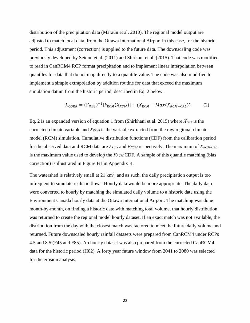
simulation datum from the historic period, described in Eq. 2 below.

F (2)

Eq. 2 is an expanded version of equation 1 from (Shirkhani et al. 2015) where Xcorr is the

corrected climate variable and XRCM is the variable extracted from the raw regional climate

model (RCM) simulation. Cumulative distribution functions (CDF) from the calibration period

for the observed data and RCM data are FOBS and FRCM respectively. The maximum of XRCM-CAL

is the maximum value used to develop the FRCM CDF. A sample of this quantile matching (bias

correction) is illustrated in Figure B1 in Appendix B.

The watershed is relatively small at 21 km2, and as such, the daily precipitation output is too

infrequent to simulate realistic flows. Hourly data would be more appropriate. The daily data

were converted to hourly by matching the simulated daily volume to a historic date using the

Environment Canada hourly data at the Ottawa International Airport. The matching was done

month-by-month, on finding a historic date with matching total volume, that hourly distribution

was returned to create the regional model hourly dataset. If an exact match was not available, the

distribution from the day with the closest match was factored to meet the future daily volume and

returned. Future downscaled hourly rainfall datasets were prepared from CanRCM4 under RCPs

4.5 and 8.5 (F45 and F85). An hourly dataset was also prepared from the corrected CanRCM4

data for the historic period (H02). A forty year future window from 2041 to 2080 was selected

for the erosion analysis.

23  

2.3.5 Hydrologic Modelling

The SWMHYMO platform (JFSA 2000) was used for the hydrologic modelling component of

this work. SWMHYMO is a lumped hydrologic model that is capable of continuous simulations

for mixed-use basins with low computational cost. Both urban (STANDHYD) and natural

(NASHYD) hydrograph generation routines are used as are channel, pipe and reservoir routing

routines. The SCS method (NRCS 2004) is used to calculate runoff excess and infiltration. The

SCS method implemented in SWMHYMO has initial abstraction as a user-defined value, this

allows the method to be used for small events, but requires a modification to the CN values

found in literature tables (NRCS 1986). Modified CN values would need to be derived if CN

were not used as a calibration variable in this work, see section 2.3.5.2. A groundwater reservoir

subroutine allows baseflow to be returned from the groundwater reservoir as runoff for natural

catchments.

The existing erosion routine was modified to implement a shear stress exceedance and

cumulative effective work method, see section 2.3.5.1 for a description of those modifications.

Details on the equations and operation of SWMHYMO are outlined in the user’s manual (JFSA

2000). A process flow chart illustrating the model interactions between the catchment

characteristics, the climate model data, the measured field data and the erosion index routine is

shown in Figure B2 in Appendix B.

2.3.5.1 Modified Erosion Index Routine

The existing erosion index routine was modified to include a subroutine to calculate shear stress

exceedance above a user-defined critical shear stress for entrainment. This routine is used to

assess existing and future erosion potential in Watts Creek.

The user defines the 1-dimensional channel characteristics of interest (channel and floodplain

slope, geometry as distance-elevation points and roughness n for the overbanks and main

channel). Within the model the routine accepts inflow hydrograph(s), on which exceedance

calculations are performed.

 

24  

The relationship between depth and flow is defined using Manning’s equation, included as Eq. 1

above. The 1-dimensional shear stress equation is used to calculate shear for a given flow, Eq. 3:

γR S (3)

In Eq. 3 above, is the bed shear stress (Pa), γ is the specific weight of water (N/m3), Rh is

hydraulic radius (m) and So is the channel slope (m/m). The work index method presented by the

Toronto and Region Conservation Authority (TRCA 2012) is an erosion indicator based on a

stream power approach, see Eq. 4:

∑ ∆ (4)

CWI is the cumulative effective work index, τc is the user-entered critical shear stress for

entrainment (Pa), τ is the bed shear stress (Pa), v is the main channel mean velocity (m/s) and Δt

is the model time step. In addition to CWI, the erosion routine calculates total hours and flow

volume in exceedance and the number of exceedance occurrences.

2.3.5.2 Hydrologic Model Setup and Calibration

Initial Model Setup

Prior to model calibration, a set of base parameters were estimated from available data or

obtained from previous studies of Watt Creek, resulting in a base model. Estimation of drainage

area (area), imperviousness (Timp), slope for impervious and pervious surfaces (SLPI and SLPP)

and reservoir characteristics are described in section 2.3.2.2. The remaining base parameters

were either set to default values or selected based on a preliminary manual calibration to improve

the goodness of fit between the base model and field flows from the DQ1 rating curve and are

then held constant during the automatic calibration process. Those parameters are as follows:

Continuous simulation parameters: time step (DT = 5 minutes) soil storage recovery rate

(SK = 0.01 mm-1), inter-event time (IET = 12 hrs) and initial abstraction recovery rates

for impervious and pervious surfaces (Ia_recimp = 6 hrs and Ia_recper 4 hrs).

25  

STANHYD parameters: Impervious and pervious surface values for; routing length (LGI

= (area [m2]/1.5)0.5 and LGP = 40 m) and initial abstraction depth (Ia_imp = 1.57 mm

and Ia_per = 4.67 mm) and surface roughness for pervious surfaces (MNP = 0.25).

NASHYD parameters: number of linear reservoirs for the Nash hydrograph (N = 3),

initial groundwater reservoir volume (InitGWResVol = 10 mm) and vertical hydraulic

conductivity (VHydCond = 0.02 mm/hr). Time to peak (tp) is calculated as 2/3 of the

time of concentration (tc). The Bransby-Williams formula (Eq. 5) was selected as the tc

method since it resulted in a relatively close match between model and field hydrograph

timing.

. ∗. . (5)

The time of concentration (tc) is in hours, catchment length (L) is in km, drainage area (A)

is in km2 and average catchment slope (S) is in percent.

Watts Creek and the Kizell drain, the largest tributary to Watts Creek, were included as route

channel commands based on the previous modelling by others with some adjustments. Channel

and overbank roughness (n) were increased for some reaches (from 0.04 to 0.085) based on 2016

field observations and to improve the model timing match to field flows. The study reach M3

geometry was updated using the 2015 RTK GPS survey data.

Generally, the timing response in the model was well fit manually. The base model had a

tendency to significantly overestimate peak flows for large events and could not match field

runoff volume for both 2015 and 2016. A close match to either year resulted in a doubling or

halving between model and field volume for the other. This mismatch between the model and the

2015 and 2016 years may have been driven by higher channel roughness in 2016 and thus the

rating curves could overestimate the 2016 peak flows and volumes. Alternately, there were

longer periods of drought in 2016, which would have led to drier antecedent conditions and

therefore less runoff volume for a given rainfall input. This may point to a structural limitation

with the hydrologic model selected given that SWMHYMO does not have input parameters that

allow for variable abstraction losses throughout a simulation, nor does the model simulate

evapotranspiration from the shallow groundwater reservoir. The results from the manual

26  

calibration effort and its uncertainty informed both the selection of a multiple model calibration

approach and specifically the six selected variable parameters. While some of the default values

used in the base model may not be fully representative of the catchment conditions, it is expected

that the variable parameters will correct for some of this potential misfit.

Handling of uncertainty in the rating curves and precipitation data

Several different calibration data sets were used to explicitly capture some of the uncertainty

introduced by the small measurement dataset which is from 2-years of data for the summer

season in the results. The more conventional approach of calibrating to part of the dataset and

comparing the results of that calibrated parameter set to the remaining data (validation) has also

been assessed. This process and the results are discussed in section 2.4.1 below. A test looking at

model performance over 40-years using the calibrated parameter sets (results not shown)

indicated that the calibrated models do not lead to divergence and thus do not suffer from

overfitting. However, due to the paucity of data, we could not identify the most representative set

of calibrated parameters. To this end, three different calibration periods were selected, and the

results from each set of calibrated parameters have been assessed. One using all field flow points

from 2015 (Y15) a second using all field points from 2016 (Y16) and a third using equal

weighting to all 2015 and 2016 data (YAL).

To capture uncertainty in the measured continuous water depth data and in using a static rating

curve for a natural channel, the set of three rating curves described previously (DQ1, DQ2 and

DQ3) were used to generate three sets of field flow data for each data period. Combined, the

three rating curves and the three calibration periods result in nine different model calibrations.

This set of models are used for the future rainfall impact assessment.

The model calibrations were performed using the Model-Independent Parameter Estimation and

Uncertainty Analysis (PEST) tool (Doherty 2016). The singular value decomposition estimation

method was used in PEST comparing the modelled continuous flow series with the field flow for

the calibration period of interest. The operation and mathematics for PEST are detailed in

(Doherty 2015).

 

27  

The multiple calibrations were conducted using the base model as the template. Three parameters

for urban catchments (STANDHYD) were allowed to vary: the SCS method infiltration

parameter (CN), percent of directly connected impervious areas (Ximp) and the impervious

surface roughness (mni). The first two parameters predominantly affect the runoff volume from

urban catchments, while the roughness for impervious surfaces will affect the hydrograph peak

and timing. The first two were allowed to vary due to complexities in estimating those values

accurately, while mni was used as a surrogate to capture inefficiencies in the drainage network.

Three parameters for natural catchments (NASHYD) were also allowed to vary. The SCS

method surface infiltration parameter (CN), rainfall initial abstraction (Ia) and the rate of

baseflow discharge from the groundwater reservoir to surface flow (gwresk). The CN value and

gwresk work in concert to control both total volume of rainfall converted to runoff, and the shape

of the hydrograph for baseflow response, particularly the recession limb. The initial abstraction

value affects runoff volume. Allowing those six parameters to vary for the urban and natural

catchments leaves the peak flows to be driven mainly by the urban areas and the baseflow and

low flow response from the natural catchments.

 

28  

2.4 Results

2.4.1 Model Calibration

The multiple rating curve and calibration period approach results in a range of peak flows and

runoff volumes for both the field and model flows for the 2015 and 2016 periods. Table I lists

the range of the field and model peak flows and runoff volumes.

Table I: Ranges of Model and Field Maximum Peak flow and total runoff volume from the 2015 and 2016 calibration periods

Year and Condition Peak Flow (m3/s)  Runoff Volume (mm) 

Low  High  Low  High 

2015 Field  3.24  3.85  64.5  75.8 

2015 Model  2.20  3.85  32.3  67.5 

2016 Field  6.51  8.24  63.8  67.2 

2016 Model  8.74  13.40  57.2  86.8 

Runoff volume is the total volume per watershed area for the simulation period.

The 2015 results show a broader span for modelled peak flow than field flow, and the range of

peak flows are completely captured. The modelled runoff volume also has a broader range,

though does not capture the highest runoff volume. In general, some of the 2015 models may

underestimate maximum peak flow and runoff volume. This trend in 2015 is offset by the 2016

data, where the model tends to overestimate peak flow and runoff volume. The highest and

lowest maximum peak flow and runoff volume values all belong to model results. The overall

broader range from the models indicates that the 9 calibration scenarios are successful in

capturing the uncertainty described by the three different rating curve approaches.

The overall efficiency or goodness of fit between the model and field flows has been assessed

using the Nash-Sutcliffe model efficiency coefficient. Table II below provides the results for the

nine model scenarios for the calibration years and the validation years when applicable.

 

 

29  

Table II: Nash-Sutcliffe model efficiency coefficient for the nine calibration scenarios and the six applicable validation scenarios

Model Scenario: Rating Curve_ Calibration Period 

Nash‐Sutcliffe model efficiency coefficient 

2015  2016 

DQ1_Y15  67%  87% 

DQ1_Y16  56%  89% 

DQ1_YAL  64%  88% 

DQ2_Y15  68%  82% 

DQ2_Y16  56%  86% 

DQ2_YAL  59%  86% 

DQ3_Y15  61%  67% 

DQ3_Y16  19%  80% 

DQ3_YAL  50%  83% 

Minimum  19%  67% 

Maximum  68%  89% 

Mean  56%  83% 

Note: the efficiency coefficient for the calibration period is shown in bold.

The naming convention for the model scenarios has the first three characters describing the

rating curve used to generate the field flow series (DQ1, DQ2 or DQ3). The second half of the

name describes the calibration period, either 2015 only (Y15), 2016 only (Y16) or all data

(YAL). The calibrations resulted in generally good matches to the calibration data, with

efficiency coefficients ranging from 61% to 89% for the individual calibration years and from

50% to 88% when both years were used to calibrate. These results were a significant

improvement over the previous manual calibration effort. As shown in Table II the ‘validation

years’ (non-bold values) show positive efficiency coefficients for the six applicable scenarios

with most being above 50% and the lowest value at 19%. These positive efficiency coefficients

for the validation runs indicate that the calibrations have not resulted in model overfitting. It is

interesting to note that the weakest match to field data occurs with DQ3, the complex rating

curve. Since this rating curve includes the field depth data, the measured water surface slope

information and a function for roughness with depth, it ought to best represent the actual creek

flows. Considering the channel routing in the SWMHYMO model, which is 1-dimensional with

a uniform flow assumption, this misfit could indicate that non-uniform flow, and perhaps

hysteresis effects, were captured by the measured water surface slope.

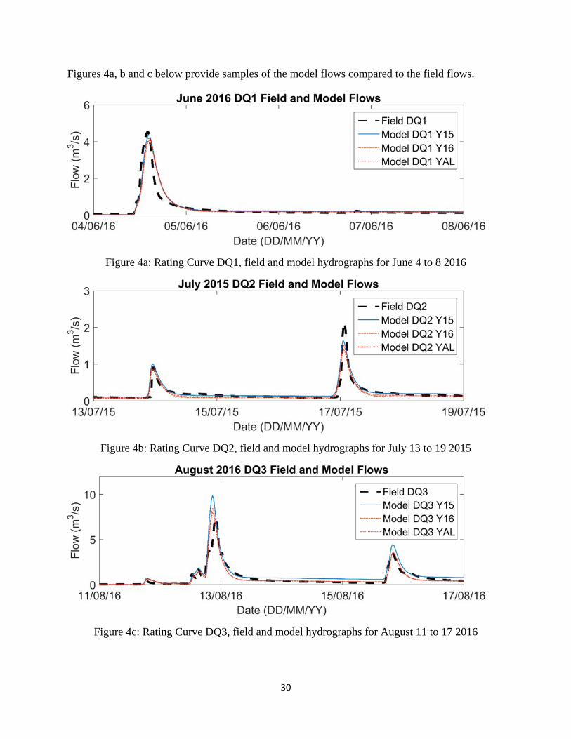
30  

Figures 4a, b and c below provide samples of the model flows compared to the field flows.

 

Figure 4a: Rating Curve DQ1, field and model hydrographs for June 4 to 8 2016

 

Figure 4b: Rating Curve DQ2, field and model hydrographs for July 13 to 19 2015

 

Figure 4c: Rating Curve DQ3, field and model hydrographs for August 11 to 17 2016

31  

Based on the breadth of the calibration results with respect to peak flows and total runoff

volumes (Table I) and the relatively high goodness of fit between the model scenarios and field

data (Table II), these nine model calibrations provide a useful envelope in which the potential

impacts of future rainfall can be assessed.

These nine models were used to generate continuous hydrographs at the study reach for the

periods when historic hourly rainfall data are available, 1968 to 2007 inclusive (excluding 2001

and 2005 due to missing data). The input rain data used for the historic runs were the hourly

rainfall data (HLY03, element 123) collected by Environment Canada at the Ottawa International

Airport Gauge, this climate dataset will be referred to as H01. The data do not include frozen

precipitation, so the model runs were constrained from April 1 to Oct 31 for each year.

2.4.2 Climate Change Projections

The same models were also used to generate future hydrographs for 2041 to 2080 under

representative concentration pathways (RCPs) 4.5 and 8.5 (F45 and F85). Another historic

climate dataset (1968 to 2007) is also considered, it is the bias corrected CanRCM4 model output

for the historic period (H02). Derivation of the regional climate model hourly rainfall datasets is

discussed in section 2.3.4.

The QQ statistical downscaling approach calculates a cumulative distribution function (CDF)

transform by fitting half of the CanRCM4 output (even years) to the station data at the Ottawa

Airport for the historic period (1961 – 2011). The odd years in the historic window are used as

the validation dataset. The same transformation is applied to the future simulation results for

RCP4.5 and RCP8.5 for the future study period of 2041-2080. A sample showing the effect of

this bias correction on monthly rainfall volume is demonstrated by Figure 5.

 

32  

 

Figure 5: Monthly Average Rainfall Volume in July, observed and modelled (raw and corrected i.e. downscaled) during historical period, as well as modelled (raw and corrected i.e.

downscaled) during future period, for calibration (even years) and validation (odd years), raw data are from CanRCM4 RCP8.5 output.

The Expert Team on Climate Change Detection and Indices (ETCCDI) provide consistent

weather metrics to assess climate change predictions across climate studies (Zhang et al. 2011).

Total annual precipitation (PRCPTOT) and number of days with rainfall exceeding 20 mm (R20)

are predicted to increase. The consecutive dry days (CDD) and wet days (CWD) show little

change, see Table III.

 

33  

Table III: Open Water Yearly Average Precipitation Indices for Historic and Future Data

Climate Dataset Name

Years PRCPTOT

(mm) CDD (days) CWD (days) R20 (days)

H01  1968‐2007  497.2  16.9  3.7  6.1 

H02  1968‐2007  581.4  17.7  4.1  7.3 

H03  1968‐2007  756.9  14.2  5.0  9.0 

H04  1968‐2007  581.5  16.5  4.1  7.1 

F45  2041‐2080  679.3  16.9  4.1  9.3 

F85  2041‐2080  724.2  17.7  4.1  10.3 

F45x  2041‐2080  667.8  16.9  4.1  9.3 

F85x  2041‐2080  702.9  17.7  4.1  10.3 

PERCENT CHANGE

F45 : H02 17% -5% 1% 27%

F85 : H02 25% 0% 1% 41%

H01: Environment Canada hourly rain data at the Ottawa International Airport (OIA) H02: CanRCM4 model output QQ bias correction to the OIA daily data H03: CanRCM4 model output without QQ bias correction H04: Environment Canada daily rain data at OIA F45: CanRCM4 model output QQ bias correction to OIA, RCP4.5 with extrapolation F85: CanRCM4 model output QQ bias correction to OIA, RCP8.5 with extrapolation F45x: CanRCM4 model output QQ bias correction to OIA, RCP4.5 no extrapolation F85x: CanRCM4 model output QQ bias correction to OIA, RCP8.5 no extrapolation Indices are calculated as yearly averages limited to the period from Apr 1 to Oct 31 inclusive for each year.

Precipitation indices are presented in Table III for the four primary climate scenarios used to

quantify the impacts of future rainfall on erosion potential in Watts Creek (H01, H02, F45 and

F85). The other four climate scenarios presented are used to: assess sensitivity to the selection of

the historic dataset, demonstrate the effect of the bias correction, and capture the sensitivity to

extrapolating RCM maxima in the downscaling process (H03, H04, F45x and F85x).

Comparing H03 and H04, we see the differences between the raw RCM output and the daily

observations at the Environment Canada gauge at the Ottawa International Airport (OIA). The

differences in total precipitation (30%) and R20 (27%) show a clear need for bias correction of

the regional model output to capture local precipitation patterns. The bias corrected RCM data

(H02) however, show a very close match with the daily station data (H04).

The effects of including the extrapolation by addition can be found by comparing F45 and F85

against their counterparts without extrapolation F45x and F85x. No differences are observed in

34  

CDD, CWD or R20, while the RCP4.5 and RCP8.5 total rainfall volume are 2% and 3% higher

than without extrapolation.

A sensitivity assessment has also been conducted from convoluting those rainfall datasets into

flow hydrographs, resultant bed shear stress and ultimately erosion indicators using the

SWMHYMO model and the modified erosion routine. Table IVa shows the results from model

WCK_DQ1_YAL (rating curve DQ1 calibrated to both 2015 and 2016) for the four historic

climate scenarios.

Table IVa: Sensitivity Assessments for Average Open Water Yearly Erosion Indicators: measured rainfall data and regional climate model with and without bias correction for the historic period (1968-2007)

Model Name Average

Flow (L/s)

Erosion Hours

(hours)*

No. of erosion events

Total Exceedance

Volume (103 m3) Ɨ

Cumulative Work Index (kPa.m or

kJ/m2)

Environment Canada hourly rainfall data vs. daily data (Ottawa International Airport). 

WCK_DQ1_YAL_H01  166 86 16 238 212

WCK_DQ1_YAL_H04  175 92 18 247 219

PERCENT DIFFERENCE  6% 7% 10% 4% 3%

Environment Canada daily station data (OIA) vs. CanRCM4 output without bias correction. 

WCK_DQ1_YAL_H04  175 92 18 247 219

WCK_DQ1_YAL_H03  234 155 25 445 409

PERCENT DIFFERENCE  34% 68% 39% 80% 87%

Environment Canada daily station data (OIA) vs. CanRCM4 output with bias correction. 

WCK_DQ1_YAL_H04  175 92 18 247 219

WCK_DQ1_YAL_H02  176 97 18 283 257

PERCENT DIFFERENCE  0% 5% 0% 14% 17%

*The rainfall input to the hydrologic model is from April 1 to Oct 31 inclusive (i.e. 5136 hours). ƗTotal exceedance volume is the cumulative flow (water) volume for flows that exceed the critical shear stress for entrainment of 3.7 Pa. H01: EC hourly station data (OIA), H02: CanRCM4 output with bias correction, H03: CanRCM4 output no bias correction, H04: EC daily station data (OIA).

The model used for these erosion indicator sensitivity assessments generates results which are

close to the mean from the nine calibrated models for both the historic and future periods. The

work index results are significantly improved between the gauge data and the regional model

output without bias correction (87% difference) and after bias correction (17% difference).

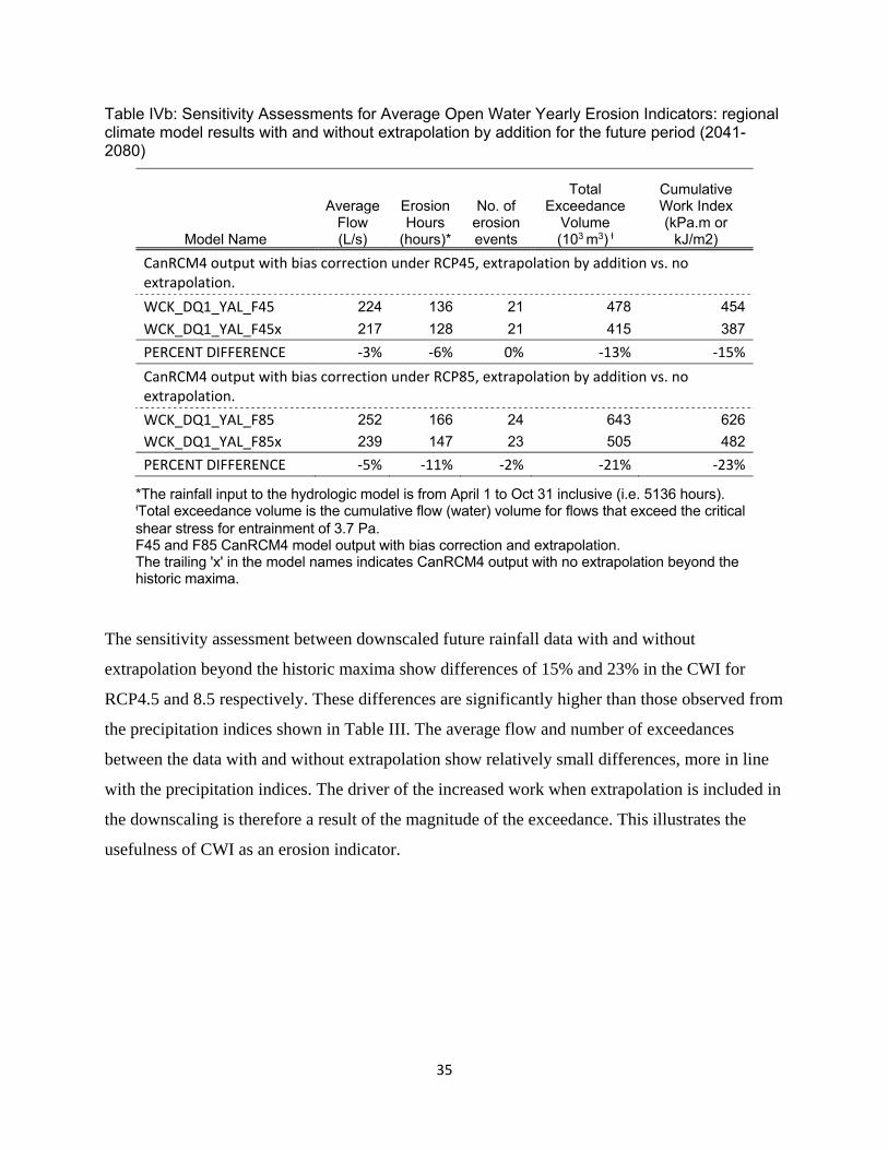
35  

Table IVb: Sensitivity Assessments for Average Open Water Yearly Erosion Indicators: regional climate model results with and without extrapolation by addition for the future period (2041-2080)

Model Name

Average Flow (L/s)

Erosion Hours

(hours)*

No. of erosion events

Total Exceedance

Volume (103 m3) Ɨ

Cumulative Work Index (kPa.m or

kJ/m2)

CanRCM4 output with bias correction under RCP45, extrapolation by addition vs. no extrapolation. 

WCK_DQ1_YAL_F45  224 136 21 478 454

WCK_DQ1_YAL_F45x  217 128 21 415 387

PERCENT DIFFERENCE  ‐3% ‐6% 0% ‐13%  ‐15%

CanRCM4 output with bias correction under RCP85, extrapolation by addition vs. no extrapolation. 

WCK_DQ1_YAL_F85  252 166 24 643 626

WCK_DQ1_YAL_F85x  239 147 23 505 482

PERCENT DIFFERENCE  ‐5% ‐11% ‐2% ‐21%  ‐23%

*The rainfall input to the hydrologic model is from April 1 to Oct 31 inclusive (i.e. 5136 hours). ƗTotal exceedance volume is the cumulative flow (water) volume for flows that exceed the critical shear stress for entrainment of 3.7 Pa. F45 and F85 CanRCM4 model output with bias correction and extrapolation. The trailing 'x' in the model names indicates CanRCM4 output with no extrapolation beyond the historic maxima.

The sensitivity assessment between downscaled future rainfall data with and without

extrapolation beyond the historic maxima show differences of 15% and 23% in the CWI for

RCP4.5 and 8.5 respectively. These differences are significantly higher than those observed from

the precipitation indices shown in Table III. The average flow and number of exceedances

between the data with and without extrapolation show relatively small differences, more in line

with the precipitation indices. The driver of the increased work when extrapolation is included in

the downscaling is therefore a result of the magnitude of the exceedance. This illustrates the

usefulness of CWI as an erosion indicator.

   

36  

2.4.3 Projected Hydrographs and Erosion

The modified erosion index routine was used to calculate historic (1968-2007) and future

(2041-2080) erosion potential through reach M3. The critical shear stress for entrainment is

estimated as 3.7 Pa. This is the average from the two samples tested from that reach by Salem et

al. (2014) and Rennie (2014). Those previous studies found significant spatial variability in bed

material critical shear stress values along Watts Creek ranging from 0.9 Pa to 5.1 Pa. Table V

shows the historic and future erosion results.

Table V: Comparison of Future and Historic Average Open Water Yearly Erosion Potential at Reach M3, Critical Shear Stress of 3.7 Pa

Climate Dataset

Name and Period*

Statistics from each DatasetƗ

Average Flow (L/s)

Exceedance Hours (hours)

No. of Exceedance

events

Total Exceedance

Volume (103 m3)

Cumulative Work Index (kPa.m or

kJ/m2)H01:

Hourly Station Data 1968-2007

Minimum 101 69 14 193 171

Maximum 201 123 21 326 289

Standard Dev. 29 16 2 41 36

Mean 161 87 17 240 213

H02: CanRCM4

1968-2007

Minimum 106 77 15 226 205

Maximum 212 151 22 397 358

Standard Dev. 31 22 2 51 46

Mean 171 100 18 285 258

F45: CanRCM4

2041-2080

Minimum 147 110 19 390 370

Maximum 264 214 26 640 599

Standard Dev. 34 31 2 74 68

Mean 217 140 22 476 450

F85: CanRCM4

2041-2080

Minimum 173 133 21 529 516

Maximum 294 270 28 849 805

Standard Dev. 35 41 2 95 86

Mean 245 170 24 635 615PERCENT CHANGE (MEAN)

F45 : H02 27% 40% 20% 67% 75%

F85 : H02 43% 70% 31% 123% 139%*The rainfall input to the hydrologic model is from April 1 to Oct 31 inclusive (i.e. 5136 hours). H01 data has missing records for 2001 and 2005. Ɨ Nine models were prepared for each climate dataset calibrating to the three (3) unique rating curves, and to three (3) different periods of field measurement data (to 2015 only, to 2016 only and to both years).

37  

Future rainfall results in increases for all erosion indicators under both climate scenarios. This

result is consistent with the precipitation index results from Table III for total precipitation and

especially for number of days with greater than 20 mm of rain.

Results for four erosion indicators, exceedance hours, number of exceedances, cumulative work

index (CWI) and total flow volume exceedance for each of the nine calibrated models in

response to four climate datasets H01, H02, F45 and F85 are presented as box and whisker plots

in Figure 6.

38  

 

Figure 6: Erosion potential indicators box and whisker plots for historic and future results. The range in average erosion indicators for the open water year (April 1st to October 31st) from each of the 9 model calibrations are shown for four climate datasets. The climate dataset names are

shown on the x-axes: H01) Historic hourly rainfall data (1968-2007), H02) CanRCM4 QQ corrected data for the historic period (1968-2007), F45) CanRCM4 RCP4.5 QQ corrected data for the future period (2041-2080) and F85) CanRCM4 RCP8.5 QQ corrected data for the future

period (2041-2080).

39  

The corrected RCM flows (H02) show higher erosion potential than the observed hourly data

(H01), though the overlap between the two is significant. The main reason for the differences are

the missing data within H01. Therefore H02 provides the most representative basis for

comparison with the predicted future data. It is important to consider the H01 data in any case,

given that this dataset is widely available for use by hydrologists.

The results of the four erosion indicators suggests that exceedance hours and number of

exceedance occurrences, if used alone, could underestimate the future increase in erosion

potential. Since the CWI method captures the magnitude of shear stress exceedance above the

threshold value, in addition to the duration and frequency of exceedance, it is a superior stand-

alone method for assessing erosion potential. It is useful to review all the indicators together

however, as frequency of exceedance and total duration can provide context for the CWI and

total exceedance volume.

The CWI results for F45 show that the predicted increase in erosion for RCP4.5 is entirely above

the uncertainty bounds of the 9 calibration models. The maximum CWI for H02 is 358 kPa.m

and the minimum for F45 is 370 kPa.m. The RCP8.5 results are higher than the F45 results,

though the upper limit of the F45 models is close to the mean from F85.

 

40  

2.5 Discussion

Previous work investigating climate change impacts on bed load transport found both positive

and negative trends depending on the studied reach (Praskievicz 2015) while Goode et al. (2013)

found an overall increase in scour potential in salmonid spawning grounds, which was partly

mitigated by biological, morphodynamic and hydraulic factors. Verhaar et al (2011) studied three

tributaries of the St. Lawrence River in response to three GCMs and found variability among

different basins and climate models, but an overall trend that high intensity events would become

more frequent. Caruso et al. (2017) found a similar overall result with variability across basins

and climate models (12 assessed) but an overall upward trend. The CanRCM4 model output have

been found to lie within the upper range of the CMIP5 ensemble (Razavi et al. 2016). So, while

variable responses have been found by other researches and it is still recommended that studies

assessing climate change impacts include more than one model scenario, one may suppose that

future downscaled CanRCM4 output would generate increased discharge and therefore increased

erosion potential, as was observed in this study.

A counterpoint to this has been shown for large watersheds where increased discharges are

expected for the winter, but decreased discharge has been predicted for the summer months

(Crossman et al. 2013; Lotsari et al. 2014). Both trends are influenced by the predicted

temperature increases from the GCMs used. We expect the importance of increased evaporation

and evapotranspiration rates to be muted however, in a highly urbanised watershed like Watts

Creek where the majority of runoff volume and peak flows are driven by the very quick response

of impervious surfaces serviced by storm sewers.

This flashy runoff behaviour is felt to limit the uncertainty introduced to this study by the use of

a hydrologic model with an initial abstraction, rather than direct evaporation, routine. Further, it

may explain the strong trend towards predicted increased runoff volume, peak flows and erosion

potential for the non-winter future periods assessed for both RCP4.5 and RCP8.5.

Sensitivity to estimate of critical shear stress

The results presented in Figure 6 and Table V depend upon the estimate of critical shear stress

for Watts Creek bed material. The measured value of τc = 3.7 Pa is reasonable for the bed

material in the study reach, nonetheless, a sensitivity test was conducted to assess the responses

41  

for τc ranging from 1 Pa to 10 Pa. This test is to acknowledge the difficulties in calculating a

precise critical shear stress for clay channels, and the high spatial variability in bed material

strength along Watts Creek.

The sensitivity analysis showed increased future erosion predictions for the entire range with the

largest increase at 7 and 8 Pa for RCP4.5. This shows that the largest increase in CWI between

future and historic flows occurred at approximately double the estimated bed material strength

for this climate scenario. The more severe RCP8.5 peaked slightly higher at 9 Pa.

The representativeness of the simulated flow and shear stress to field conditions is assessed by

considering the reach bankfull characteristics. The bankfull level was estimated in the field

where an abrupt change in cross slope and vegetation cover was observed. The bankfull depth is

approximately 1.1 m at WC4. Parsapour-Moghaddam et al. (2015) measured a flow of 1,368 L/s,

a thalweg depth of 1.1 m, and estimated this flow to be just below bankfull. Therefore, the

bankfull discharge is approximately 1,400 L/s. For the 3.7 Pa estimate of bed strength, the

erosion index routine calculated an equivalent flow of 900 L/s. Conversely, the model finds a

discharge of 1,400 L/s for a critical shear stress of 4.5 Pa. Assuming that the shear stress at

bankfull flow corresponds to the critical shear stress for entrainment, this result suggests that

either the bed material strength may be greater than 3.7 Pa, or the measured water surface slope

through the reach at bankfull flow may be overestimated.

In any case, a range of 22% between simulated bed shear stress at bankfull flow and the average

of the measured bed material shear stress for entrainment is a relatively good match. Further, the

maximum measured bed strength along Watts Creek was 5.1 Pa (Salem et al. 2014; Rennie

2014), greater than simulated shear stress at the model-estimated bankfull flow. Therefore, the

simulated critical shear results correspond fairly well with the visual estimate of bankfull

discharge, suggesting that 3.7 Pa is a useful estimate for the strength of the controlling bed layer

in this reach and that the model produces a reasonable relationship between flow and erosion

potential.

Consideration of channel adjustment

While this study uses continuous hydrographs to assess erosion in response to the full range of

summer hydrographs, it does not include a morphodynamic routine. To estimate future channel

42  

adjustment, a sensitivity analysis that balances future erosion potential with historic erosion

potential, was implemented. Several erosion index commands with increasingly larger channel

dimensions than the current Watts Creek WC4 section were included in the SWMHYMO input

files. The critical shear stress for entrainment was maintained at 3.7 Pa for these wider channel

segments. The results were processed to assess which increased channel shape would result in

the same work above threshold (CWI) under future flows as is observed for the existing channel

under historic flows.

In this sensitivity analysis for channel adjustment, the concepts of bankfull flow and bankfull

geometry are useful classification tools. This method for estimating channel growth in response

to increased average work during open water yearly conditions yields an increased top (bankfull)

width of 2.4 m for RCP4.5 and an increase of 4.1 m for RCP8.5. The current channel has an

estimated bankfull width of 6.1 m and bankfull depth of 1.1 m. This assessment of increased

width with a stable depth has been considered for two reasons. First, the channel hydraulics in

the erosion routine assume uniform flow and thus, are not adequate to assess the hydraulic

complexities that arise from local channel deepening. Second, and perhaps more importantly for

this particular case, there are twin circular 2.3 m diameter concrete culverts located

approximately 170 m downstream from the channel section of interest. The hard-bottom of those

culverts act as control on the Watts Creek profile through reach M3, and thus deepening to

reduce erosive work may occur locally within the reach, but is not an available mechanism to

reduce erosion potential for the reach in general.

Another factor that suggests widening may be the dominant form of channel adjustment in the

future is the current hydraulic geometry of the section. Previous work on downstream hydraulic

geometry of semi-alluvial (clay) channels in the Ottawa region found a range of bankfull width

to depth ratios of 7.8 to 30.4, with a mean of 16.2 (Ebisa Fola & Rennie 2010). Compared to that

range, the observed width to depth ratio for section WC4 in Watts Creek is very low at 5.5 and

thus may tend to a wider configuration.

While our model does not have a lateral channel migration routine, the channel adjustment

sensitivity analysis approach proposed above quantifies potential future channel widening. In a

review on the prospects and challenges of predicting river change in response to a changing

climate Lotsari et al. (2015) pose an open question on whether the research community should

43  

focus on enhancing multi-dimensional modelling (example 2-D and 3-D) or instead work on

improving 1-D models to include morphodynamic routines. They conclude by proposing an

idealised model for future analyses would be: 2-D, morphodynamic, unsteady and capable of

simulating the century scale. This is left as a future objective for the research community. In the

meantime, a simpler approach, like the one presented in this study, may be a straightforward and

useful step for the river management community. This may be particularly true for works

affecting small watercourses where schedule and time constraints for studies can be quite strict.

Uncertainty

Uncertainty in the collected data and hydrologic modelling has been managed to some extent

through the multiple model calibrations. Uncertainty in the regional climate model output is

reduced by considering two RCPs and through the quantile matching to rainfall data at the

Ottawa Airport. Significant uncertainty remains in the process nonetheless, particularly with

respect to estimates of both historic and future erosion rates. A threshold model for erosion

analysis is common and can provide useful comparative results, but is a simplification of the

erosion process particularly for semi-alluvial channels. Therefore, the erosion results generally

and the predicted channel widening specifically, cannot be expected to predict future geomorphic

change with a high degree of accuracy, though they can be used to predict the expected trend in

response to climate change and as a comparative result for assessing usefulness of mitigation

measures or sensitivity to other future rainfall scenarios.

 

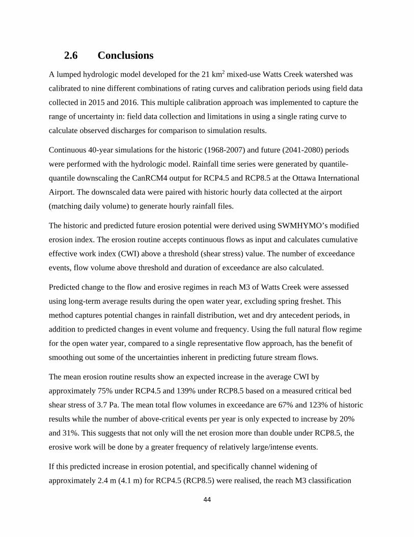
44  

2.6 Conclusions

A lumped hydrologic model developed for the 21 km2 mixed-use Watts Creek watershed was

calibrated to nine different combinations of rating curves and calibration periods using field data

collected in 2015 and 2016. This multiple calibration approach was implemented to capture the

range of uncertainty in: field data collection and limitations in using a single rating curve to

calculate observed discharges for comparison to simulation results.

Continuous 40-year simulations for the historic (1968-2007) and future (2041-2080) periods

were performed with the hydrologic model. Rainfall time series were generated by quantile-

quantile downscaling the CanRCM4 output for RCP4.5 and RCP8.5 at the Ottawa International

Airport. The downscaled data were paired with historic hourly data collected at the airport

(matching daily volume) to generate hourly rainfall files.

The historic and predicted future erosion potential were derived using SWMHYMO’s modified

erosion index. The erosion routine accepts continuous flows as input and calculates cumulative

effective work index (CWI) above a threshold (shear stress) value. The number of exceedance

events, flow volume above threshold and duration of exceedance are also calculated.

Predicted change to the flow and erosive regimes in reach M3 of Watts Creek were assessed

using long-term average results during the open water year, excluding spring freshet. This

method captures potential changes in rainfall distribution, wet and dry antecedent periods, in

addition to predicted changes in event volume and frequency. Using the full natural flow regime

for the open water year, compared to a single representative flow approach, has the benefit of

smoothing out some of the uncertainties inherent in predicting future stream flows.

The mean erosion routine results show an expected increase in the average CWI by

approximately 75% under RCP4.5 and 139% under RCP8.5 based on a measured critical bed

shear stress of 3.7 Pa. The mean total flow volumes in exceedance are 67% and 123% of historic

results while the number of above-critical events per year is only expected to increase by 20%

and 31%. This suggests that not only will the net erosion more than double under RCP8.5, the

erosive work will be done by a greater frequency of relatively large/intense events.

If this predicted increase in erosion potential, and specifically channel widening of

approximately 2.4 m (4.1 m) for RCP4.5 (RCP8.5) were realised, the reach M3 classification

45  

would change from relatively stable to unstable. Increased erosion would increase sediment load

in the creek, which could be harmful for fish habitat, and would also pose increased risk to

nearby infrastructure. These results suggest the need for further study to understand in more

detail what the potential effects could be and how to either mitigate them or adapt. Particularly,

future work is being considered to include the winter season and spring freshet in the hydrologic

modelling and couple the resulting hydrographs with a 3-D morphodynamic and habitat

suitability model.

 

46  

3 Thesis Conclusions

This work has put forward a modelling approach to assess the impacts of climate change on clay-

bed stream erosion at the local scale for a small urban catchment. The numerically efficient

process produces hourly distributions of predicted future rainfall that are sufficiently resolved for

hydrologic modelling. The newly implemented stream-power-based Erosion Index routine

enhances the usefulness of the SWMHYMO hydrologic platform to assess erosion potential. The

numerical efficiency of SWMHYMO allows one to assess erosion response to multiple years

(1,440 for this study) of continuous rainfall and flow output while having the flexibility to

implement a channel adjustment sensitivity analysis approach, which balances future erosion

potential with historic erosion potential, to estimate future channel enlargement.

This process, and the addition of the new Erosion Index routine to SWMHYMO, will be of

benefit to river engineers particularly for studying clay-bed (semi-alluvial) stream behaviour for

ungauged urban watercourses. Cohesive bed, ungauged and urbanised watercourses are common

in the Ottawa area and other parts of Canada that were subject to glaciation.

The predicted future precipitation from CanRCM4 under RCP4.5 and RCP8.5 from 2041-2080

were downscaled to the EC gauge at the Ottawa International Airport. Rainfall data from that

gauge are used as a standard in the City of Ottawa for both continuous hourly historic

simulations and to derive local intensity duration frequency (IDF) curves. The future data were

converted from daily to hourly time series and formatted to meet Environment Canada’s HLY03

element 123 format. These future precipitation datasets could be easily incorporated into

hydrologic and river engineering studies by practitioners, consultants or researchers interested in

the Ottawa area and climate change.

For Watts Creek specifically, the impacts of climate change in the 2041 – 2080 period could

result in significantly more erosion than today, 75% under RCP4.5 and 139% under RCP8.5. The

channel adjustment sensitivity analysis approach gives an estimated increase in channel width of

2.1 m and 4.1 m respectively compared to the current bankfull width of 6.1 m. The next question

would be, what should we do about this potential increased erosion risk, which could put

infrastructure at risk and would harm aquatic habitat? After all, a widening from about 6 m to

10 m seems like a major morphological change. For the sediment transport regime and aquatic

47  

habitat it certainly would be, but what about infrastructure? Perhaps the answer can be found in

river management rather than engineering. If we consider no-touch offsets for infrastructure

adjacent to watercourses (i.e. a corridor where no physical modifications to the landscape or

construction are permitted), maybe we should just give small channels enough space and not

impinge on their floodways and natural meander belts. From that perspective, a 4 m change

seems quite manageable for a City of 2,700 km2 and especially for a country that is about

9.9 M km2.

Considerations toward improved planning would not, however address the risks to existing

nearby infrastructure or aquatic habitat. A finer understanding of the mechanics of the current

and projected future erosion in Watts Creek should be studied to understand how to mitigate

those risks.

3.1 Recommendations for Future Work

The research program for this thesis comprised two main segments, a field work component and

a numerical modelling component. In reflecting on these efforts and the strengths and

weaknesses of the study, some recommendations for improvement come to mind. For the field

program, improved accuracy and scope would be beneficial. Water depths were measured

continuously at the upstream and downstream end of an approximately 80 m reach. More

observation points should be considered to measure the local water surface slopes more

accurately, particularly for low flows. Depths were field verified regularly (every 2 or 3 weeks)

to corroborate the continuous measurements. The water surface slope measurements should be

verified in the field with the same frequency as the depth verification, rather than simply using

temporary benchmarks as the reference measure. For such a short reach, a simple rod and level

survey is straightforward to implement and can provide high accuracy measurement for small

(<10 cm) changes in elevation. The study scope included no- ice-covered conditions and rainfall

as the only precipitation measure, model runs were constrained between April 1st and October

31st of each year. Spring freshet conditions could be incorporated via snowpack monitoring and

depth (flow) gauging starting in March or April. A snowmelt and rain routine could be added to

SWMHYMO, or other software could be incorporated into the process. On the modelling side,

while a channel adjustment sensitivity analysis was implemented, a direct 1-dimensional

morphodynamic model (with a lateral migration subroutine) driven by sediment transport

48  

relationships could be included. A morphodynamic model would increase computational cost,

but the process could still be more efficient than higher order modelling. A comparison between

the 1-dimensional morphodynamic solution and the channel adjustment sensitivity analysis

SWMHYMO approach would be useful. Finally, two climate scenarios were considered (RCP45

and 85) both from the same RCM (CanRCM4). The analysis, particularly the uncertainty

component, would be improved by assessing future precipitation from more climate scenarios.

Beyond those fairly straightforward recommendations, there are many factors that affect

hydrodynamics and channel morphology that are dynamic in both time and space. Accounting

for these complexities would provide a more rounded and complete analysis.

Luhar et al. (2008) studied the interaction of vegetation patches on relative channel roughness

and found that sufficiently dense vegetation patches prevent turbulence from reaching the bed,

i.e. the underlying bed material is virtually unerodable when covered by patches of dense

vegetation. Related work (Green 2005; Luhar and Nepf 2013) proposed a field and numerical

approach to estimate roughness relative to vegetative growth. They proposed that the seasonal

vegetation changes that drive roughness should be incorporated dynamically into future

modelling studies. While this would be both field and model intensive, it may allow for a greater

understanding of erosive and hydraulic mechanics. Further, these methods could be expanded to

include an additive strength term, as vegetation grows to cover the bare bed in the early spring to

densely vegetated in the mid to late summer for example. Based on qualitative field observations,

the bed and banks of Watts Creek are bare in the spring. In patches, the bed becomes densely

vegetated and likely unerodable in the summer. The banks, particularly at the toe, remain bare

and show signs of active erosion via mass wasting (pock marks with exposed smooth

unweathered clay material). This bank undercutting was previously observed by Rennie (2014)

and Parsapour-Moghaddam et al. (2015). There may be two distinct periods of channel

adjustment, incising into the bare bed material driven by high spring freshet flows and then

widening via bank undercutting once vegetation has become established. The channel geometry

indicates that historically the dominant process has been incision. The existing bankfull width to

depth ratio at reach M3 is 5.5. This is very low compared to the range for semi-alluvial (clay)

channels in the Ottawa area 7.8 to 30.4 found in (Ebisa Fola & Rennie 2010).

49  

Future work is being considered to use the continuous hydrographs generated from the calibrated

hydrologic models as input to a 3-D morphodynamic and habitat suitability study. Given the

complexities of clay-bed morphology and the seasonal effects of vegetation on roughness and

erodibility this higher level modelling should provide a better understanding of how Watts Creek

is evolving today and what the future may bring. This refined information could inform

mitigation measures to protect aquatic habitat and infrastructure.

The hourly future precipitation (rain) data from CanRCM4 downscaled to the Ottawa

International Airport gauge for RCP4.5 and RCP8.5 have potential usefulness for the river

engineering and research communities as described previously. While two climate scenarios

have been assessed, similar datasets should be prepared from other climate models, both RCMs

and GCMs. This would allow future studies to capture the sometimes divergent predictions and

uncertainty inherent in climate modelling. The approach could also be implemented for locations

across the province and country where sufficient historic hourly precipitation data are available

(minimum 20-years of hourly data). The climate change web based IDF tool by (Simonovic et al.

2016) may provide a useful template for how to accomplish this geographically broad

downscaling task while making the data readily available to the river engineering community.

 

50  

References

AECOM. (2015). Shirley’s Brook & Watt’s Creek Phase 2 Stormwater Management Study. Report prepared by AECOM for the City of Ottawa, Ottawa, Canada.

Alodah, A. (2015). Development of Climate Change Scenarios for the South Nation Watershed. M.A.Sc. Thesis, Civil Engineering, University of Ottawa.

Arcement, G. J. J., & Schneider, V. R. (1989). Guide for Selecting Manning’s Roughness Coefficients for Natural Channels and Flood Plains. Washington, DC: GPO. http://doi.org/Report No. FHWA-TS-84-204

Bagnold, R. A. (1966). An approach to the sediment transport problem from general physics. Physiographic and hydraulic studies of rivers Geological Survey Professional Paper 422-1. Washington, DC: GPO.

Benestad, R. E., Hanssen-Bauer, I., & Forland, J. (2007). An evaluation of statistical models for downscaling precipitation and their ability to capture long-term trends. International Journal Of Climatology, 27, 649–665. http://doi.org/10.1002/joc.1421

Bussi, G., Dadson, S. J., Prudhomme, C., & Whitehead, P. G. (2016). Modelling the future impacts of climate and land-use change on suspended sediment transport in the River Thames (UK). Journal of Hydrology, 542, 357–372. http://doi.org/10.1016/j.jhydrol.2016.09.010

Carter, T. R., Parry, M. L., Harasawa, H., & Nishioka, S. (1994). IPCC Technical Guidelines for Assessing Climate Change Impacts and Adaptations, special report to Working group II. Intergov. Panel on Climate Change.

Caruso, B., Newton, S., King, R., & Zammit, C. (2017). Modelling climate change impacts on hydropower lake inflows and braided rivers in a mountain basin. Hydrological Sciences Journal, 62(6), 928–946. http://doi.org/10.1080/02626667.2016.1267860

Canadian Council of Resource and Environment Ministers (CCREM) (1987). Freshwater Aquatic Life. In Canadian Environmental Quality Guidelines, Ottawa, Canada: Environment Canada.

Canadian Council of Ministers of the Environment (CCME) (2002). Total particulate matter. In Canadian Water Quality Guidelines for the Protection of Aquatic Life, Ottawa, Canada: Environment Canada.

City of Ottawa. (2014). Report to Environment Committee. Retrieved from http://app05.ottawa.ca/sirepub/cache/2/j12ytbc4v2owa2zwngsmzi3n/10570509102017105220192.PDF

Coulthard, T. J., Ramirez, J., Fowler, H. J., & Glenis, V. (2012). Using the UKCP09 probabilistic scenarios to model the amplified impact of climate change on drainage basin sediment yield. Hydrology and Earth System Sciences, 16(11), 4401–4416. http://doi.org/10.5194/hess-16-4401-2012

Croke, J., Fryirs, K., & Thompson, C. (2016). Defining the floodplain in hydrologically-variable settings: implications for flood risk management. Earth Surface Processes and Landforms, 41(14), 2153–2164. http://doi.org/10.1002/esp.4014

Crossman, J., Futter, M. N., Oni, S. K., Whitehead, P. G., Jin, L., Butterfield, D., Dillon, P. J. (2013). Impacts of climate change on hydrology and water quality: Future proofing management strategies in the Lake Simcoe watershed, Canada. Journal of Great Lakes Research, 39(1), 19–32. http://doi.org/10.1016/j.jglr.2012.11.003

Diplas, P., Dancey, C. L., Celik, A. O., Valyrakis, M., Greer, K., & Akar, T. (2008). The Role of

51  

Impulse on the Initiation of Particle Movement Under Turbulent Flow Conditions. Science, 322(5902), 717–720. http://doi.org/10.1126/science.1158954

Doherty, J. (2015). Calibration and Uncertainty Analysis for Complex Environmental Models. Brisbane, Australia: Watermark Numerical Computing.

Doherty, J. (2016). PEST Model-Independent Parameter Estimation User Manual Part I: PEST, SENSAN and Global Optimisers. Brisbane, Australia: Watermark Numerical Computing.

Dust, D., & Wohl, E. (2012). Conceptual model for complex river responses using an expanded Lane’s relation. Geomorphology, 139–140, 109–121. http://doi.org/10.1016/j.geomorph.2011.10.008

Ebisa Fola, M., & Rennie, C. D. (2010). Downstream Hydraulic Geometry of Clay-Dominated Cohesive Bed Rivers. Journal of Hydraulic Engineering, 136(8), 524–527. http://doi.org/10.1061/(ASCE)HY.1943-7900.0000199

Einstein, H. (1950). The bed-load function for sediment transportation in open channel flows. 1026. Soil Conservation Service. Washington, DC: GPO.

Environment and Climate Change Canada. (2014). Climate Modelling and Analysis Canadian Centre for Climate Modelling and Analysis. Retrieved January 1, 2015, from http://ec.gc.ca/ccmac-cccma/default.asp?lang=en&n=82DD0FCC-1

Escauriaza, C., & Sotiropoulos, F. (2011). Initial stages of erosion and bed form development in a turbulent flow around a cylindrical pier. Journal of Geophysical Research: Earth Surface, 116(3), 1–24. http://doi.org/10.1029/2010JF001749

Fowler, H. J., & Wilby, R. L. (2007). Beyond the downscaling comparison study. International Journal Of Climatology, 27, 1543–1545. http://doi.org/10.1002/joc.1616

Goode, J. R., Buffington, J. M., Tonina, D., Isaak, D. J., Thurow, R. F., Wenger, S., … Soulsby, C. (2013). Potential effects of climate change on streambed scour and risks to salmonid survival in snow-dominated mountain basins. Hydrological Processes, 27(5), 750–765. http://doi.org/10.1002/hyp.9728

Green, J. C. (2005). Effect of macrophyte spatial variability on channel resistance. http://doi.org/10.1016/j.advwatres.2005.05.010

Hammer, T. R. (1972). Stream Channel Enlargment Due to Urbanization. Water Resources Research, 8(6), 1530–1540

Huth, R. (2002). Statistical downscaling of daily temperature in central Europe. Journal of Climate, 15(13), 1731–1742.

IPCC. (2012). Managing the Risks of Extreme Events and Disasters to Advance Climate Change Adaptation. A Special Report of Working Groups I and II of the Intergovernmental Panel on Climate Change. (C. B. Field, V. Barros, T.F. Stocker, D. Qin, D.J. Dokken, K.L. Ebi, … P.M. Midgley, Eds.). Cambridge: Cambridge University Press.

IPCC. (2014). Climate Change 2014: Synthesis Report. Contribution of Working Groups I, II and III to the Fifth Assessment Report of the Intergovernmental Panel on Climate Change. (The Core Writing Team, R. K. Pachauri, & L. A. Meyer, Eds.)Core Writing Team, R.K. Pachauri and L.A. Meyer. Geneva, Switzerland: IPCC. http://doi.org/10.1017/CBO9781107415324.004

J.F. Sabourin and Associates Inc. (JFSA) (2000). SWMHYMO User’s Manual. Ottawa, Canada: JFSA.

Jeong, D. I., St-Hilaire, A., Ouarda, T. B. M. J., & Gachon, P. (2013). A multi-site statistical downscaling model for daily precipitation using global scale GCM precipitation outputs. International Journal Of Climatology, 33, 2431–2447. http://doi.org/10.1002/joc.3598

52  

King, L. M., Irwin, S., Sarwar, R., McLeod, a. I., & Simonovic, S. P. (2012). The Effects of Climate Change on Extreme Precipitation Events in the Upper Thames River Basin: A Comparison of Downscaling Approaches. Canadian Water Resources Journal, 37(3), 253–274. http://doi.org/10.4296/cwrj2011-938

Knighton, D. (1998). Fluvial Forms and Processes. London, UK: Arnold. Kundzewicz, Z. W., Mata, L. J., Arnell, N. W., Döll, P., Jimenez, B., Oki, T., Shiklomanov, I.

(2008). The implications of projected climate change for freshwater resources and their management resources and their management. Hydrological Sciences Journal, 53(1), 3–10. http://doi.org/10.1623/hysj.53.1.3

Laforce, S., Simard, M. C., Leconte, R., & Brissette, F. (2011). Climate change and floodplain delineation in two southern quebec river basins. Journal of the American Water Resources Association, 47(4), 785–799. http://doi.org/10.1111/j.1752-1688.2011.00560.x

Lane, S. N., Bakker, M., Gabbud, C., Micheletti, N., & Saugy, J. N. (2016). Sediment export, transient landscape response and catchment-scale connectivity following rapid climate warming and Alpine glacier recession. Geomorphology, 277, 210–227. http://doi.org/10.1016/j.geomorph.2016.02.015

Lenderink, G., & van Meijgaard, E. (2008). Increase in hourly precipitation extremes beyond expectations from temperature changes. Nature Geoscience, 1(8), 511–514. http://doi.org/10.1038/ngeo262

Li, H., Sheffield, J., & Wood, E. F. (2010). Bias correction of monthly precipitation and temperature fields from Intergovernmental Panel on Climate Change AR4 models using equidistant quantile matching. Journal of Geophysical Research Atmospheres, 115(10). http://doi.org/10.1029/2009JD012882

Li, Z., & Fang, H. (2016). Impacts of climate change on water erosion: A review. Earth Science Reviews, 163, 94–117. http://doi.org/10.1016/j.earscirev.2016.10.004

Lotsari, E., Aaltonen, J., Veijalainen, N., Alho, P., & Käyhkö, J. (2014). Future fluvial erosion and sedimentation potential of cohesive sediments in a coastal river reach of SW Finland. Hydrological Processes, 28, 6016–2037. http://doi.org/10.1002/hyp.10080

Lotsari, E., Thorndycraft, V., & Alho, P. (2015). Prospects and challenges of simulating river channel response to future climate change. Progress in Physical Geography, 39(4), 483–513. http://doi.org/10.1177/0309133315578944

Luhar, M., & Nepf, H. M. (2013). From the blade scale to the reach scale: A characterization of aquatic vegetative drag. Advances in Water Resources, 51, 305–316. http://doi.org/10.1016/j.advwatres.2012.02.002

Luhar, M., Rominger, J., & Nepf, H. (2008). Interaction between flow, transport and vegetation spatial structure. Environ Fluid Mech, 8, 423–439. http://doi.org/10.1007/s10652-008-9080-9

Maarschalk-Bliss, S. (2014). Seasonal Variation in Assemblage Structure and Movement of Small Stream Fish in an Urban Environment. M.S. Thesis, Biology, Carleton University.

Maraun, D., Wetterhall, F., Chandler, R. E., Kendon, E. J., Widmann, M., Brienen, S., Thiele-Eich, I. (2010). Precipitation downscaling under climate change: Recent developements to bridge the gap between dynamical models and the end user. Reviews of Geophysics, 48(RG3003), 1–38. http://doi.org/10.1029

Mcmillan, H., Freer, J., Pappenberger, F., Krueger, T., & Clark, M. (2010). Impacts of uncertain river flow data on rainfall-runoff model calibration and discharge predictions. Hydrological Processes, 24, 1270–1284. http://doi.org/10.1002/hyp.7587

53  

Mehrotra, R., & Sharma, A. (2015). Correcting for systematic biases in multiple raw GCM variables across a range of timescales. Journal of Hydrology, 520, 214–223. http://doi.org/10.1016/j.jhydrol.2014.11.037

Mehrotra, R., & Sharma, A. (2016). A multivariate quantile-matching bias correction approach with auto- and cross-dependence across multiple time scales: implications for downscaling. Journal of Climate, 29(10), 3519–3539. http://doi.org/10.1175/JCLI-D-15-0356.1

Molnar, P. (2001). Climate change, flooding in arid environments, and erosion rates. Geology, 29(12), 1071–1074. http://doi.org/10.1130/0091-7613(2001)029<1071:CCFIAE>2.0.CO

MTO. (1997). Drainage Management Manual. Ministry of Transportation Ontario. Toronto, Canada: Queen's Printer for Ontario.

Muste, M., & Hoitink, A. J. F. (2017). Continuous streamflow monitoring using stage measurements. In J. Aberle, C. D. Rennie, D. M. Admiraal, & M. Muste (Eds.) Experimental Hydraulics Volume II (pp. 7.15 – 7.24). New York, USA: Taylor & Francis.

Nam, D. H., Udo, K., & Mano, A. (2015). Future fluvial flood risks in Central Vietnam assessed using global super-high-resolution climate model output. Journal of Flood Risk Management, 8(3), 276–288. http://doi.org/10.1111/jfr3.12096

Nanson, G. C., & Croke, J. C. (1992). A genetic classification of floodplains. Geomorphology, 4(6), 459–486. http://doi.org/10.1016/0169-555X(92)90039-Q

Naylor, L. A., Spencer, T., Lane, S. N., Darby, S. E., Magilligan, F. J., Macklin, M. G., & Möller, I. (2017). State of Science Stormy geomorphology: geomorphic contributions in an age of climate extremes. Earth Surface Processes and Landforms, 42, 166–190. http://doi.org/10.1002/esp.4062

NRCS, USDA. (1986). Estimating Runoff, In Urban Hydrology for Small Watersheds (2nd ed., pp. 2.1 – 2.16). Washington, DC: GPO.

NRCS, USDA. (2004). Estimation of Direct Runoff from Storm Rainfall. In National Engineering Handbook (pp. 10.1 – 10.21) . Washington, DC: GPO.

Ontario Ministry of Agriculture Food and Rural Affairs. (1999). Provincial Landcover 2000 - 27 Classes. Retrieved June 3, 2015, from https://www.ontario.ca/page/land-information-ontario

Ontario Ministry of Agriculture Food and Rural Affairs. (2015). Soil Survey Complex. Retrieved December 1, 2015, from https://www.ontario.ca/page/land-information-ontario

Parker, G. (2003). Bed load at low Shields stress on arbitrarily sloping beds: Alternative entrainment formulation. Water Resources Research, 39(7), 1–11. http://doi.org/10.1029/2001WR001253

Parsapour-Moghaddam, P., Rennie, C. D., Midwood, J., Cvetkovic, M., & Cooke, S. J. (2015). Influence of Channel Erosion on Fish Habitat Utilization. In 36th IAHR World Congress, Hague, Netherlands.

Praskievicz, S. (2014). Impacts of projected climate changes on streamflow and sediment transport for three snowmelt-dominated rivers in the interior Pacific Northwest. River Research and Applications, 32, 4–17. http://doi.org/10.1002/rra.2841

Praskievicz, S., & Bartlein, P. (2014). Hydrologic modeling using elevationally adjusted NARR and NARCCAP regional climate-model simulations: Tucannon River, Washington. Journal of Hydrology, 517, 803–814. http://doi.org/10.1016/j.jhydrol.2014.06.017

Praskievicz, S. (2015). A coupled hierarchical modeling approach to simulating the geomorphic response of river systems to anthropogenic climate change. Earth Surface Processes and Landforms, 40(12), 1616–1630. http://doi.org/10.1002/esp.3740

Rajczak, J., Kotlarski, S., & Schär, C. (2016). Does quantile mapping of simulated precipitation

54  

correct for biases in transition probabilities and spell lengths? Journal of Climate, 29(5), 1605–1615. http://doi.org/10.1175/JCLI-D-15-0162.1

Rantz, S. E. (1982). Measurement and computation of stream flow: Volume 2. Computation of Discharge. US Geological Survey water-supply paper 2175 (Vol. 2175). http://doi.org/10.1029/WR017i001p00131

Razavi, T., Switzman, H., Arain, A., & Coulibaly, P. (2016). Regional climate change trends and uncertainty analysis using extreme indices: A case study of Hamilton, Canada. Climate Risk Management, 13, 43–63. http://doi.org/10.1016/j.crm.2016.06.002

Rennie, C. D. (2014). Linking sediment erodibility and channel stability to utilization of available habitats. Report written by the University of Ottawa for the National Capital Commission, Ottawa, Canada.

Richter, B. D., Baumgartner, J. V, Powell, J., & Braun, D. P. (1996). Society for Conservation Biology A Method for Assessing Hydrologic Alteration within Ecosystems. Conservation Biology, 10(4), 1163–1174.

Richardson, J.R., Richardson, E.V. (2008). Bridge Scour Evaluation. In M. Garcia (Ed.) Sedimentation Engineering: Processes, Measurements, Modeling, and Practice (pp. 505 – 542). Virginia, USA: ASCE.

Rummukainen, M. (1997). Methods for statistical downscaling of GCM simulations. Rep. Meteorol. Climatol. Norrköping. Retrieved from http://agris.fao.org/agris-search/search/display.do?f=2012/OV/OV201205379005379.xml;SE19970167745

Salem, H. (S.), Rennie, C. D., & Custodio, C. Z. (2014). Influence of Pore Pressure on Clay Erosion. In River Flow 2014. Lausanne, Switzerland.

Schmeeckle, M. W. (2014). Numerical simulation of turbulence and sediment transport of medium sand. Journal of Geophysical Research: Earth Surface, 119(6), 1240–1262. http://doi.org/10.1002/2013JF002911

Schmeeckle, M. W., & Nelson, J. M. (2003). Direct numerical simulation of bedload transport using a local, dynamic boundary condition. Sedimentology, 50(2), 279–301. http://doi.org/10.1046/j.1365-3091.2003.00555.x

Shields, A. (1936). Anwendung der Ähnlichkeitsmechanik und der Turbulenzforschung auf die Geschiebebewegung. Mitteilung Der Preußischen Versuchsanstalt Für Wasserbau Und Schiffbau, Heft 26. Berlin.

Scinocca, J. F., Kharin, V. V., Jiao, Y., Qian, M. W., Lazare, M., Solheim, L., Dugas, B. (2015). Coordinated Global and Regional Climate Modeling. Journal of Climate, 29(1), 17–35. http://doi.org/10.1175/JCLI-D-15-0161.1

Seidou, O., Ramsay, A., & Nistor, I. (2011). Climate change impacts on extreme floods II: improving flood future peaks simulation using non-stationary frequency analysis. Nat Hazards, 60(2), 715–726. http://doi.org/10.1007/s11069-011-0047-7

Shirkhani, H., Seidou, O., Mohammadian, A., & Qiblawey, H. (2015). Projection of Significant Wave Height in a Coastal Area under RCPs Climate Change Scenarios. Natural Hazards Review, 17(1), 04015016–1:15. http://doi.org/10.1061/(ASCE)NH.1527-6996.0000192

Shrestha, B., Babel, M. S., Maskey, S., Van Griensven, A., Uhlenbrook, S., Green, A., & Akkharath, I. (2013). Impact of climate change on sediment yield in the Mekong River basin: A case study of the Nam Ou basin, Lao PDR. Hydrology and Earth System Sciences, 17(1), 1–20. http://doi.org/10.5194/hess-17-1-2013

Simonovic, S. P., Schardong, A., & Sandink, D. (2016). Mapping Extreme Rainfall Statistics for Canada under Climate Change Using Updated Intensity-Duration-Frequency Curves.

55  

Journal of Water Resources Planning and Management, 143(3), 1–12. http://doi.org/10.1061/(ASCE)WR.1943-5452 .0000725.

Teng, J., Potter, N. J., Chiew, F. H. S., Zhang, L., Wang, B., Vaze, J., & Evans, J. P. (2015). How does bias correction of regional climate model precipitation affect modelled runoff? Hydrology and Earth System Sciences, 19(2), 711–728. http://doi.org/10.5194/hess-19-711-2015

The Federal Interagency Stream Restoration Working Group (FISRWG) (15 Federal agencies of the US gov’t). (1998). Stream Corridor Restoration, Principles, Processes, and Practices. Washington, DC: GPO.

Thorne, C.R. (1982). Processes and mechanisms of river bank erosion. In R.D. Hey, J.C. Bathurst, and C.R. Thorne (Eds.) Gravel bed rivers (227-272). Chichester, England: Wiley.

Toronto and Region Conservation Authority. (2012). Stormwater Management Criteria. Toronto, Canada: Author.

Trapp, R. J., Diffenbaugh, N. S., Brooks, H. E., Baldwin, M. E., Robinson, E. D., & Pal, J. S. (2007). Changes in severe thunderstorm environment frequency during the 21st century caused by anthropogenically enhanced global radiative forcing. Proceedings of the National Academy of Sciences , 104(50), 19719–19723. http://doi.org/10.1073/pnas.0705494104

Verhaar, P. M., Biron, P. M., Ferguson, R. I., & Hoey, T. B. (2011). Implications of climate change in the twenty-first century for simulated magnitude and frequency of bed-material transport in tributaries of the Saint-Lawrence River, 25, 1558–1573. http://doi.org/10.1002/hyp.7918

Walker, J. F., Hay, L. E., Markstrom, S. L., & Dettinger, M. D. (2011). Characterizing Climate-Change Impacts on the 1.5-yr Flood Flow in Selected Basins across the United States: A Probabilistic Approach. Earth Interactions, 15(18), 1–16. http://doi.org/10.1175/2010EI379.1

Widmann, M., Bretherton, C. S., & Salathé, E. P. (2003). Statistical precipitation downscaling over the northwestern united states using numerically simulated precipitation as a predictor. Journal of Climate, 16(5), 799–816. http://doi.org/10.1175/1520-0442(2003)016<0799:SPDOTN>2.0.CO;2

Wilby, R. L., & Wigley, T. M. L. (1997). Downscaling general circulation model output: a review of methods and limitations. Progress in Physical Geography, 21(4), 530–548.

Wilby, R. L., & Wigley, T. M. L. (2000). Precipitation predictors for downscaling: Observed and general circulation model relationships. International Journal of Climatology, 20(6), 641–661. http://doi.org/10.1002/(SICI)1097-0088(200005)20:6<641::AID-JOC501>3.0.CO;2-1

Wilcock, P. R., & Crowe, J. C. (2003). Surface-based transport model for mixed-size sediment. Journal of Hydraulic Engineering, 129(2), 120–128. http://doi.org/10.1061/(ASCE)0733-9429(2003)129:2(120)

Williams, R.D., Rennie, C.D., Brasington, J., Hicks, M., Vericat, D. (2015) Linking the spatial distribution of bedload transport to morphological change during high-flow events in a shallow braided river, J. Geophysical Research – Earth Surface, 120, 604–622, doi:10.1002/2014JF003346.

Wolman, M. G., & Miller, J. P. (1960). Magnitude and Frequency of Forces in Geomorphic Processes. The Journal of Geology, 68(1), 54–74.

Yellen, B., Woodruff, J. D., Cook, T. L., & Newton, R. M. (2016). Historically unprecedented erosion from Tropical Storm Irene due to high antecedent precipitation. Earth Surface Processes and Landforms, 41(5), 677–684. http://doi.org/10.1002/esp.3896

56  

Zhang, X., Alexander, L., Hegerl, G. C., Jones, P., Tank, A. K., Peterson, T. C., Zwiers, F. W. (2011). Indices for monitoring changes in extremes based on daily temperature and precipitation data. Wiley Interdisciplinary Reviews: Climate Change, 2(6), 851–870. http://doi.org/10.1002/wcc.147

 

57  

Appendix A: Depth, Rain, Flow and Creek profile data collected for Watts Creek

Figure A1: 2015 depths at sections WC3 and WC4 (upstream and downstream ends of reach M3) and rainfall data for Watts Creek for June, July and August

Figure A2: 2016 depths at sections WC3 and WC4 (upstream and downstream ends of reach M3) and rainfall data for Watts Creek for June, July and August

Figure A3: 2015 field flow at WC4 from rating curve DQ1 and rainfall data for Watts Creek for June, July and August

Figure A4: 2016 field flow at WC4 from rating curve DQ1 and rainfall data for Watts Creek for June, July and August

Table A1: Discharge measurements collected in Watts Creek

Figure A5: Discharge measurements collected in Watts Creek

Figure A6: Watts Creek thalweg profile from reach M3 to the downstream rail crossing

 

58  

Figure A1: 2015 depths at sections WC3 and WC4 (upstream and downstream ends of reach M3) and rainfall data for Watts Creek for June, July and August. The thalweg inverts are: 69.70 masl at WC3 and 69.61 masl at WC4 (see Figure A6).

59  

Figure A2: 2016 depths at sections WC3 and WC4 (upstream and downstream ends of reach M3) and rainfall data for Watts Creek for June, July and August. The thalweg inverts are: 69.70 masl at WC3 and 69.61 masl at WC4 (see Figure A6).

 

60  

 

Figure A3: 2015 field flow at WC4 from rating curve DQ1 and rainfall data for Watts Creek for June, July and August.

 

61  

Figure A4: 2016 field flow at WC4 from rating curve DQ1 and rainfall data for Watts Creek for June, July and August.

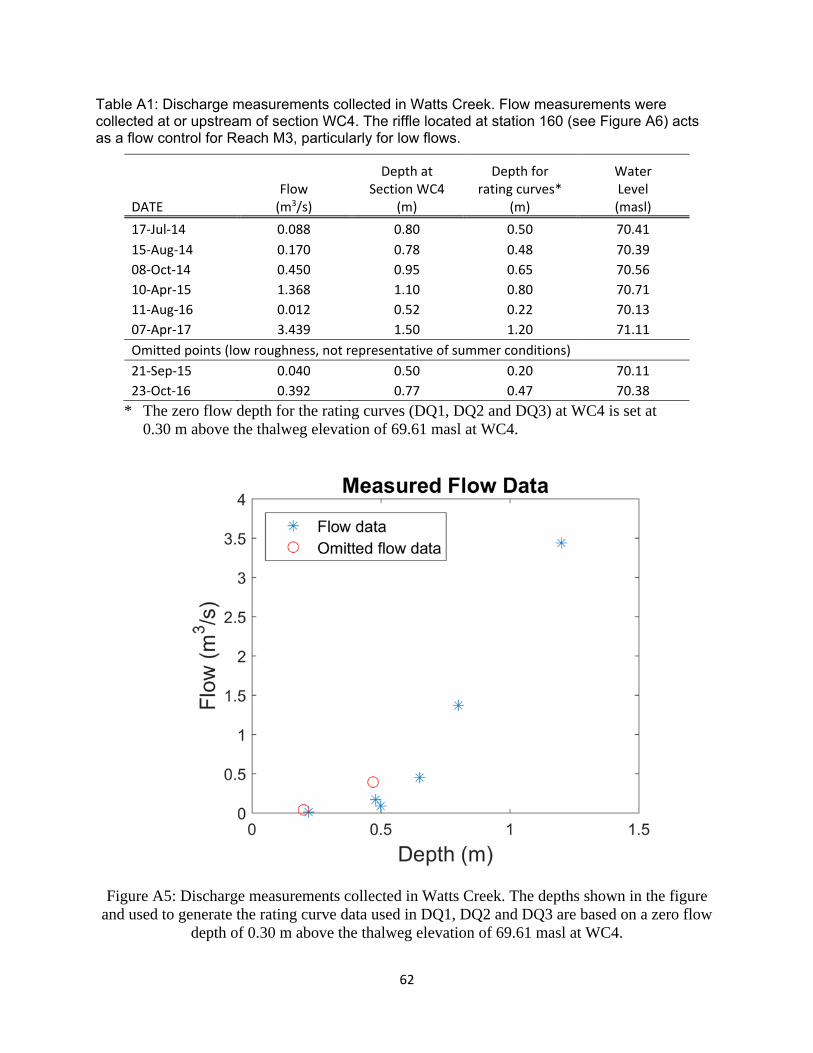
62  

Table A1: Discharge measurements collected in Watts Creek. Flow measurements were collected at or upstream of section WC4. The riffle located at station 160 (see Figure A6) acts as a flow control for Reach M3, particularly for low flows.

DATE Flow  (m3/s) 

Depth at Section WC4 

(m) 

Depth for  rating curves* 

(m) 

Water  Level  (masl) 

17‐Jul‐14  0.088  0.80  0.50  70.41 

15‐Aug‐14  0.170  0.78  0.48  70.39 

08‐Oct‐14  0.450  0.95  0.65  70.56 

10‐Apr‐15  1.368  1.10  0.80  70.71 

11‐Aug‐16  0.012  0.52  0.22  70.13 

07‐Apr‐17  3.439  1.50  1.20  71.11 

Omitted points (low roughness, not representative of summer conditions) 

21‐Sep‐15  0.040  0.50  0.20  70.11 

23‐Oct‐16  0.392  0.77  0.47  70.38 

* The zero flow depth for the rating curves (DQ1, DQ2 and DQ3) at WC4 is set at 0.30 m above the thalweg elevation of 69.61 masl at WC4.

Figure A5: Discharge measurements collected in Watts Creek. The depths shown in the figure and used to generate the rating curve data used in DQ1, DQ2 and DQ3 are based on a zero flow

depth of 0.30 m above the thalweg elevation of 69.61 masl at WC4.

63  

Figure A6 – Watts Creek thalweg profile from reach M3 to the downstream rail crossing. Section WC3 is at station 289 m, shown by a vertical dotted black line and WC4 is at station 200 m, shown by a vertical dashed black line. The thalweg elevations along reach M3 were surveyed using a total station, the approximate thalweg elevations between the total station survey extent and the downstream

culvert are based on depth estimates at: the culvert upstream invert; the riffles at stations 70 m and 160 m and at WC4 on August 10, 2016. The culvert invert elevations are from (AECOM 2015). The channel flow direction is from right to left.

64  

Appendix B: Quantile quantile transform schematic and modelling process flow chart

Figure B1: Schematic illustrating the quantile-quantile transform using CanRCM 4 data and Environment Canada data from the Ottawa International Airport, bias correction, before extrapolation by addition

Figure B2: Modelling process flow chart

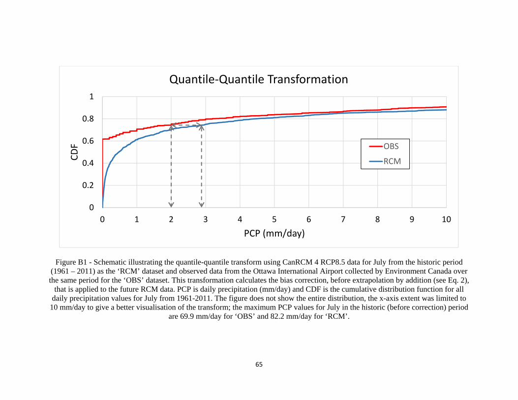
65  

Figure B1 - Schematic illustrating the quantile-quantile transform using CanRCM 4 RCP8.5 data for July from the historic period (1961 – 2011) as the ‘RCM’ dataset and observed data from the Ottawa International Airport collected by Environment Canada over the same period for the ‘OBS’ dataset. This transformation calculates the bias correction, before extrapolation by addition (see Eq. 2),

that is applied to the future RCM data. PCP is daily precipitation (mm/day) and CDF is the cumulative distribution function for all daily precipitation values for July from 1961-2011. The figure does not show the entire distribution, the x-axis extent was limited to

10 mm/day to give a better visualisation of the transform; the maximum PCP values for July in the historic (before correction) period are 69.9 mm/day for ‘OBS’ and 82.2 mm/day for ‘RCM’.

0

0.2

0.4

0.6

0.8

1

0 1 2 3 4 5 6 7 8 9 10

CDF

PCP (mm/day)

Quantile‐Quantile Transformation

OBS

RCM

66  

Figure B2 – Modelling process flow chart illustrating the model interactions between the catchment characteristics, the climate model data, the measured field data and the erosion index

routine.