River discharge to the Baltic Sea in a future climate

Chantal Donnelly & Wei Yang & Joel Dahné

Received: 13 November 2012 /Accepted: 17 September 2013 /Published online: 17 November 2013# The Author(s) 2013. This article is published with open access at Springerlink.com

Abstract This study reports on new projections of discharge to the Baltic Sea given possiblerealisations of future climate and uncertainties regarding these projections. A high-resolution,pan-Baltic application of the Hydrological Predictions for the Environment (HYPE) model wasused to make transient simulations of discharge to the Baltic Sea for a mini-ensemble of climateprojections representing two high emissions scenarios. The biases in precipitation and temper-ature adherent to climate models were adjusted using a Distribution Based Scaling (DBS)approach. As well as the climate projection uncertainty, this study considers uncertainties in thebias-correction and hydrological modelling. While the results indicate that the cumulativedischarge to the Baltic Sea for 2071 to 2100, as compared to 1971 to 2000, is likely to increase,the uncertainties quantified from the hydrological model and the bias-correction method showthat even with a state-of-the-art methodology, the combined uncertainties from the climatemodel, bias-correction and impact model make it difficult to draw conclusions about themagnitude of change. It is therefore urged that as well as climate model and scenario uncer-tainty, the uncertainties in the bias-correction methodology and the impact model are also takeninto account when conducting climate change impact studies.

1 Introduction

How discharge to the Baltic Sea will change is a significant uncertainty regarding future climatein the Baltic Sea region (Meier et al. 2006). For example, this is of particular interest whenconsidering changes to salinity levels in the sea which has implications for the sea’s uniqueecosystem. Changes in precipitation (P), temperature (T) and evapotranspiration (E) in a futureclimate affect generation of runoff (R), and the resulting discharge, (Q). Studies to date,including regional climate studies and impact studies on the catchment hydrology and BalticSea ecosystems were summarised in 2008 (BACC Author Team 2008). Previously publishedstudies have predicted net changes in total Q to the Baltic Sea ranging from around −14 to +33 % (Graham 2004; Meier et al. 2006; Hansson et al. 2011; Hagemann et al. 2012).Nevertheless, methods used to make impact studies have progressed since the aforementionedstudies for this region.

Climatic Change (2014) 122:157–170DOI 10.1007/s10584-013-0941-y

C. Donnelly (*) :W. Yang : J. DahnéSwedish Meteorological and Hydrological Institute, 1 Folkborgsvägen, 60176 Norrköping, Swedene-mail: Chantal.donnelly@gmail.com

W. Yange-mail: wei.yang@smhi.se

J. Dahnée-mail: joel.dahne@smhi.se

Previous estimates of total changes to Q to the Baltic Sea have been taken directly fromglobal climate models (GCMs) or regional climate models (RCMs) using simple water balancecalculations from the climate model outputs (e.g. P – E, e.g. IPCC 2001; Meleshko et al. 2004)or runoff output directly from climate models (e.g. Hagemann et al. 2009). Evaluations of GCMand RCM outputs show strong biases for present climate, such as overestimation of P andWinter T in parts of Northern Europe (Kjellström et al. 2010) and systematic overestimation ofE from RCMs for the Baltic Basin (Graham et al. 2007). Furthermore a large-scale calculationof mean annual (P – E) has insufficient representation of hydrological storage in snow,groundwater, lakes and magazines to resolve seasonal and spatial differences. This has beenhandled by applying routing to RCM model outputs, e.g. Hagemann and Dumenil (1999) andGraham et al. (2007); however, these studies are still subject to the aforementioned biases fromthe climate models.

An alternative is statistical downscaling of air temperature atmospheric indices to total Qto the Baltic Sea (Hansson et al. 2011). Simplified extrapolation of this technique to futureclimates suggested 8–14 % reduction in total annual Q based on predicted increase intemperature of 3–5 °C for 2100; however changes in atmospheric indices in future climatewere not considered. The regression model works well for the Northern and Southern Balticregion, but poorly in the Gulf of Finland where two large lakes result in a more complexsystem with lag and dampening effect.

To include the effects of routing and hydrological storage, hydrological models can be used.Graham (2004) set up the HBV model to calculate monthly inflows to the Baltic Sea, for fourdifferent climate projections using a delta-change method to account for biases in precipitationand temperature from climate models. This study was extended to 16 climate projections withpredicted change in total Q ranging from −8 % to 26 % (Meier et al. 2006). Recently Omstedtet al. (2012), showed results of two climate change scenarios corrected using delta-change toforce a lumped conceptual hydrological model set-up for 82 rivers and 35 coastal areas for theBaltic Sea catchment. Both these projections also indicated increases in Q to the Baltic Sea.

State-of-the-art in simulating the impact of CC on Q for large river basins is similar to thatdescribed above and includes perturbing an observed forcing data set with a future climatechange predicted by a GCM or RCM (Yukon River: Hay and McCabe 2010; Danube basin:Kling et al. 2012) or using raw RCM outputs (Colorado River: Gao et al. 2011). The delta-change method is a conventionally used approach when conducting CC impact studies. It iseasy to implement; however it is unable to deal with covariance and the variability ofweather variables in future climate (Graham et al. 2007), hence the need for bias correction(BC) techniques. Most state-of-the-art catchment scale studies use more advanced BCmethods for correcting RCM outputs to force offline hydrological models (e.g. Olssonet al. 2011; Hurkmans et al. 2010; Fowler et al. 2007); however few of these consider theuncertainties arising from BC or the HM.

Large-scale hydrological models (spanning multiple catchments) and land-surfaceschemes are emerging for use in CC impact studies (e.g. Van Vliet et al. 2012) along withbias-corrected forcing data. Although such models cannot reproduce Q to the performancelevels of catchment scale models simultaneously in all catchments within the domain, theyallow for studies over large regions (e.g. Arnel 1999; Van Vliet et al. 2012). A recent globalscale climate change study where eight global hydrological models (GHMs) were forced bythree GCMs and two emissions scenarios suggested that uncertainty in Q was relativelyconstrained for the Baltic Sea basin (Hagemann et al. 2012). Nevertheless, the predictedvariation in change to Baltic Sea Q predicted by the 8 GHMs ranged from around −3 % to +33 % of today’s Q, which is larger than the uncertainty shown by previous estimates basedon a single hydrological model (e.g. Meier et al. 2006).

158 Climatic Change (2014) 122:157–170

This new, regional study for the Baltic Sea basin uses a pan-Baltic application of theHYPE model (Lindström et al. 2010) to simulate the effects of a mini-ensemble of five bias-corrected climate projections representing variations of business-as-usual conditions onfreshwater influxes to the Baltic Sea. New to this study is that transient estimates of Q tothe Baltic Sea are made using bias-corrected RCM forcing in a large-scale (multi-basin)hydrological model, Balt-HYPE, with sufficient resolution to respond to the spatial variationin climate impacts. Rather than simulating a large ensemble such as done in previous studiesfor the region (e.g. Meier et al. 2006), emphasis was put on updating the methodology usedto estimate Q change to the Baltic Sea and investigating relative uncertainties. The impact ofuncertainty due to the hydrological model is not usually accounted for in climate changeimpact studies (Hagemann et al. 2012). Hagemann et al. (2012) addressed this by using anensemble of GHMs, but in this study, the magnitude of the uncertainty from a singlehydrological model and the BC methodology is discussed in relation to the spread of resultsfor the simulated climate scenarios. The methods shown here could be used to estimatechanges to and uncertainties in Q for other large scale river basins and the basins of otherenclosed seas such as the Black Sea or the Mediterranean Sea, where few similar studies forthe whole sea’s catchments have been made.

2 Data and methods

2.1 Hydrological model and its setup

A high-resolution, process based hydrological and nutrient flux model was set up for the Baltic Seacatchment using the HYPE model (Lindström et al. 2010), a semi-distributed, process basedhydrological and nutrient model. It shares some similarities to the HBV (Bergström 1976), VIC(Liang et al. 1994) and SWAT (Arnold et al. 1994) models. The major hydrological processessimulated by the model are snow accumulation and snowmelt, evapotranspiration, surface runoff,macropore flow, tile drainage, groundwater outflow from soil layers, routing through rivers andretention and outflow from lakes and reservoirs, both natural and regulated. Calculations are madefor unique Soil and Land Cover classes (SLC classes) at the subbasin scale; flow is then routedbetween subbasins. The model input data sources are summarised in Table 1. The model was set upwith a median subbasin resolution of 325 km2. Daily river discharge data from the BALTEX(BHDC2009) andGRDC (2009) databaseswas used to calibrate and validate parameters describinghydrological processes. The period 1980 to 2004 was used for both calibration and validationbecause this was the period of availability of the hindcast forcing data.

Calibration of the model made use of the concept of Representative Gauged Basins (RGBs,Strömqvist et al. 2012). Groups of RGBs for each soil-type had (a) limited effect of lakes, i.e.<1% lake area, and (b) dominance of soil-type of interest, i.e. at least >50% of the gauged basinarea. A simple manual calibration was then done by optimising five parameters (for fieldcapacity, effective porosity, recession in soil layers, and tile drains) for each group, i.e. for thecoarse grained soils RGB, parameters were optimised by looking graphically at performanceand at the correlation coefficient (r), relative error (RE) and Nash-Sutcliffe error (NSE)simultaneously for the group. Because a group of basins is calibrated simultaneously, there isa compromise in model performance at a single site, to optimise performance for the wholegroup. Nevertheless, these compromises are commonly accepted in large-scale modelling (e.g.Vörösmarty et al. 1989; Arnel 1999). In total 35 stations were used in calibration.

To determine whether the calibrated model was capable of reproducing spatial and temporalvariability in Q to the Baltic Sea, model performance at 31 stations near the Baltic coastline was

Climatic Change (2014) 122:157–170 159

evaluated by looking at the monthly NSE, RE and the Pearson correlation coefficient (r) at eachstation. Even if a bias (indicated by RE) exists at a station, it is the relative change inQwhich isof interest in this climate change study, so the correlation coefficient (r) gives a relevantmeasureof the model’s ability to reproduce the processes that drive variability in the catchment. Becausethis study focuses on change to total Q to the Baltic Sea, the reproduction of the seasonal andtotal Q to the Baltic Sea was also compared with observations and previous studies.

2.2 Bias correction methodology

Distribution-Based Scaling aims to adjust systematic bias in GCM/RCM outputs whilstpreserving the temporal variability in meteorological variables resulting from climate pro-jections. Comparable to other well-known quantile-mapping methods (Piani et al. 2010;Themeßl et al. 2010), DBS implements parametric distributions to describe the variables ofinterest to correct the variable outside the reference period. Additionally, co-variationbetween P and T is taken into consideration.

Adjusting precipitation is a two-step process: 1) days with precipitation < threshold arechanged to 0 mm to match the observed percentage of wet days (RCMs tend to generatespurious ‘drizzle’); 2) precipitation is transformed to match the observed frequency distri-bution. Normal and extreme precipitation events are separated by a 95th percentile valuecalculated from the whole precipitation series. Their main properties are captured byimplementing a double-gamma distribution. Considering the dependency between precipi-tation and temperature, the systematic bias in temperature is adjusted conditioned on the wetor dry state of the day. The conditioned temperature is then fitted to a normal distributionwhose distribution parameters are smoothed using a 15-day moving window and describedby Fourier series. Details can be found in Yang et al. (2010).

2.3 Future climate projections

The calibrated and validated model, Balt-HYPE, was then used to simulate the impacts of amini-ensemble of five downscaled climate projections. These projections were chosen byMeier et al. (2011) to represent two high emissions scenarios (business-as-usual), aspects ofGCM uncertainty and those GCMs that performed best for the Baltic Sea region. Four of thefive projections were downscaled using RCAO to 25 km (Meier et al. 2011) while the fifth wasregionally downscaled to 50 km using the RCA3 model (Kjellström et al. 2010). The scenarioschosen are denoted as RCAOE5A1B1, RCAOE5A1B3, RCAOE5A2, RCAOH3A1B and

Table 1 Summary of Balt-HYPEmodel data inputs and set up Data type Details (source)

Areal extent 1,8 million km2

Median Subbasin Resolution 325 km2

No. Subbasins 5128

Topography/routing Hydro1K (USGS 2000)

Precipitation andTemperature Data

ERAMESAN 1980–2004, Janssonet al. (2007), Resolution=11 km.

Landcover Globcover 2000 (GLC 2009)

Soil types European Soils Database (JRC 2006)

Discharge measurements GRDC (GRDC 2009), BALTEX(BHDC 2009)

160 Climatic Change (2014) 122:157–170

RCA3E5A1B3 where E5 and H3 denote the ECHAM5 (Jungclaus et al. 2006) and HadleyCM3 (Collins et al. 2010) GCMs respectively, and A1B and A2 denote emissions scenariosfrom the IPCC representing rapid economic growth and a differentiated world, respectively(Nakicenovic and Swart 2000). Roughly this represents business-as-usual. Although thisensemble is not large enough to constrain all the climate model or emissions uncertainty, it isuseful to analyse some of the sources of uncertainty and relate hydrological model uncertaintyto climate model uncertainty.

Five transient, daily simulations from 1971 to 2100 (with spin-up 1961 to 1970) weremade. To facilitate comparison of the projections with each other and previous studies, meanannual values of P, T, local runoff (R) and Q were calculated for a reference period (1971 to2000) and a future period (2071 to 2100). Hydrological changes were then defined as thedifference between mean annual values for the future period (called P2) and the referenceperiod (called P1). Percent changes were calculated as this change divided by the P1 meanvalue×100 %.

3 Results

3.1 Model validation

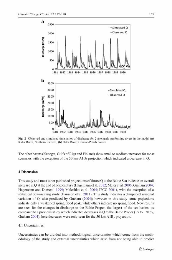
For stations to sea, median values of performance across the 31 stations were: RE: −2.0%, dailyr: 0.78 and monthlyNSE: 0.51%.Most (>75%) stations could be simulated to within 15% RE,r>0.7 and NSE >0.4. Spatial variations in performance are shown in Fig. 1. Spread of resultsacross stations can be attributed to limitations in input data and calibration when setting up alarge-scale hydrological model, particularly biases in the gridded precipitation data and abilityto simulate anthropogenic water management (e.g. poorer NSE in regulated rivers). Totalsimulated Q to the Baltic Sea, 15,609 m3/s, compared well to that estimated by Bergströmand Carlsson (1994) who estimated a total Q of 15,310m3/s based on observations in filled withsimulated data from the HBV model. Seasonal distribution of total Q to the Baltic Sea was alsowell reproduced by themodel (Fig. 1d). There is a small overestimation of runoff between June andDecember and an underestimation for January to April. Figure 2 shows simulated and observedflow for two averagely performing rivers in the model, the Kalix River and the Oder River.

3.2 Bias-correction of the climate projections

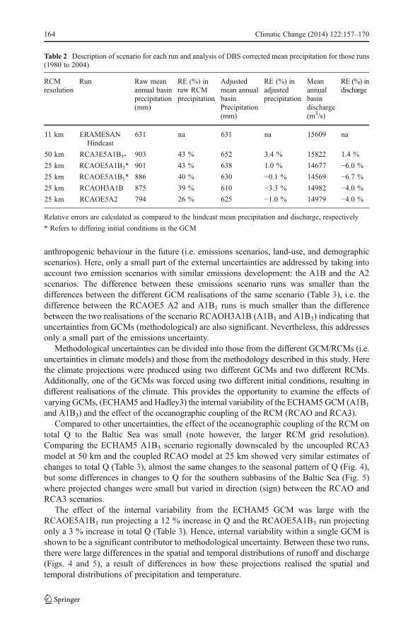
The DBS bias-correction (BC) was tuned for the period 1980 to 2004. Table 2 shows themean annual basin precipitation during the tuning period for each of the raw and correctedensemble members and the discharge using corrected precipitation. There is still a small bias(up to +/−3 %) in the total corrected precipitation across the basin which results in biases inQ of up to 7 %. Nevertheless, this is much less than the biases had the raw climate data beenused (26 to 43 %) and it is also seen that DBS significantly improves the distribution ofprecipitation and resulting discharge events (e.g. for RCAOE5A1B3, Fig. 3). This result wasrepresentative for all the scenarios.

3.3 Projections of future discharge

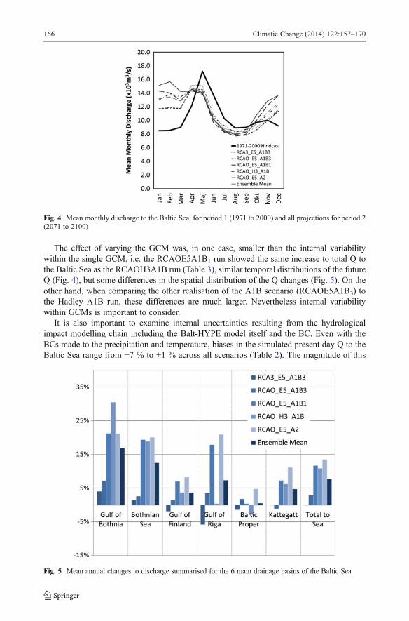
All projections indicate increases in average Q to the Baltic Sea ranging from 1 % to 14 % bythe end of the century with an ensemble average of +8 % (Table 3). For all projectionsseasonal dynamics of Q to the Baltic Sea are expected to change considerably compared to

Climatic Change (2014) 122:157–170 161

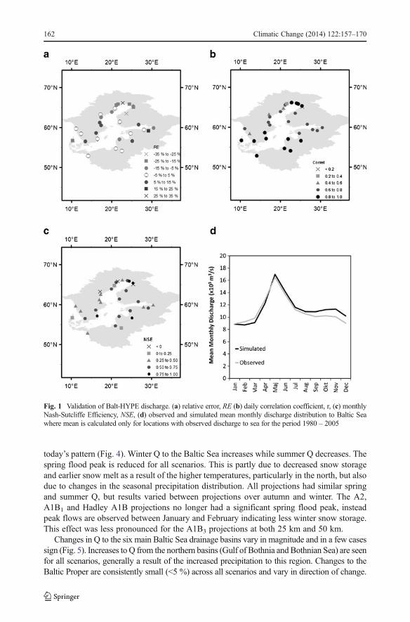
today’s pattern (Fig. 4). Winter Q to the Baltic Sea increases while summer Q decreases. Thespring flood peak is reduced for all scenarios. This is partly due to decreased snow storageand earlier snow melt as a result of the higher temperatures, particularly in the north, but alsodue to changes in the seasonal precipitation distribution. All projections had similar springand summer Q, but results varied between projections over autumn and winter. The A2,A1B1 and Hadley A1B projections no longer had a significant spring flood peak, insteadpeak flows are observed between January and February indicating less winter snow storage.This effect was less pronounced for the A1B3 projections at both 25 km and 50 km.

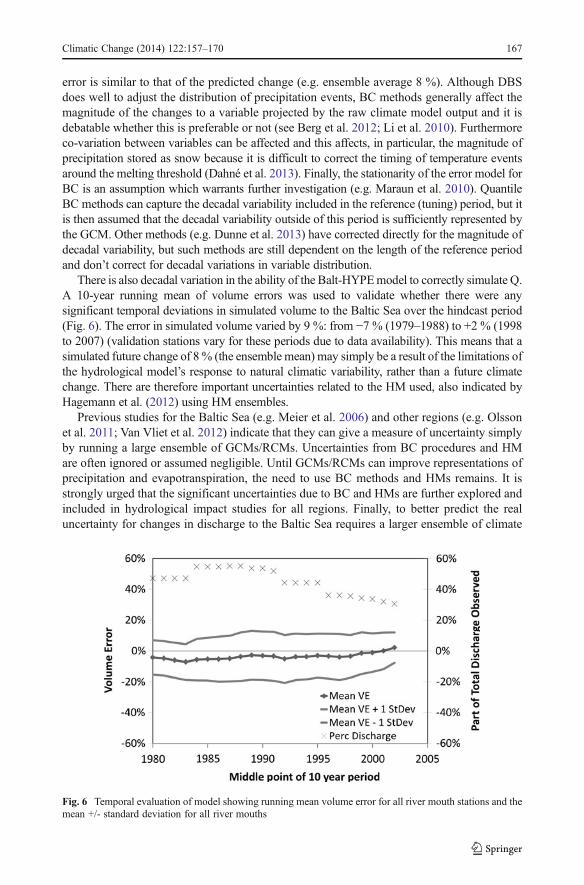
Changes in Q to the six main Baltic Sea drainage basins vary in magnitude and in a few casessign (Fig. 5). Increases to Q from the northern basins (Gulf of Bothnia andBothnian Sea) are seenfor all scenarios, generally a result of the increased precipitation to this region. Changes to theBaltic Proper are consistently small (<5 %) across all scenarios and vary in direction of change.

Fig. 1 Validation of Balt-HYPE discharge. (a) relative error, RE (b) daily correlation coefficient, r, (c) monthlyNash-Sutcliffe Efficiency, NSE, (d) observed and simulated mean monthly discharge distribution to Baltic Seawhere mean is calculated only for locations with observed discharge to sea for the period 1980 – 2005

162 Climatic Change (2014) 122:157–170

The other basins (Kattegat, Gulfs of Riga and Finland) show small to medium increases for mostscenarios with the exception of the 50 km A1B3 projection which indicated a decrease in Q.

4 Discussion

This study and most other published projections of future Q to the Baltic Sea indicate an overallincrease in Q at the end of next century (Hagemann et al. 2012;Meier et al. 2006; Graham 2004;Hagemann and Dumenil 1999; Meleshko et al. 2004; IPCC 2001), with the exception of astatistical downscaling study (Hansson et al. 2011). This study indicates a dampened seasonalvariation of Q, also predicted by Graham (2004); however in this study some projectionsindicate only a weakened spring flood peak, while others indicate no spring flood. New resultsare seen for the changes in discharge to the Baltic Proper, the largest of the sea basins, ascompared to a previous study which indicated decreases in Q to the Baltic Proper (−5 to −30%,Graham 2004); here decreases were only seen for the 50 km A1B3 projection.

4.1 Uncertainties

Uncertainties can be divided into methodological uncertainties which come from the meth-odology of the study and external uncertainties which arise from not being able to predict

Fig. 2 Observed and simulated time-series of discharge for 2 averagely performing rivers in the model (a)Kalix River, Northern Sweden, (b) Oder River, German/Polish border

Climatic Change (2014) 122:157–170 163

anthropogenic behaviour in the future (i.e. emissions scenarios, land-use, and demographicscenarios). Here, only a small part of the external uncertainties are addressed by taking intoaccount two emission scenarios with similar emissions development: the A1B and the A2scenarios. The difference between these emissions scenario runs was smaller than thedifferences between the different GCM realisations of the same scenario (Table 3), i.e. thedifference between the RCAOE5 A2 and A1B1 runs is much smaller than the differencebetween the two realisations of the scenario RCAOH3A1B (A1B1 and A1B3) indicating thatuncertainties from GCMs (methodological) are also significant. Nevertheless, this addressesonly a small part of the emissions uncertainty.

Methodological uncertainties can be divided into those from the different GCM/RCMs (i.e.uncertainties in climate models) and those from the methodology described in this study. Herethe climate projections were produced using two different GCMs and two different RCMs.Additionally, one of the GCMs was forced using two different initial conditions, resulting indifferent realisations of the climate. This provides the opportunity to examine the effects ofvarying GCMs, (ECHAM5 and Hadley3) the internal variability of the ECHAM5GCM (A1B1

and A1B3) and the effect of the oceanographic coupling of the RCM (RCAO and RCA3).Compared to other uncertainties, the effect of the oceanographic coupling of the RCM on

total Q to the Baltic Sea was small (note however, the larger RCM grid resolution).Comparing the ECHAM5 A1B3 scenario regionally downscaled by the uncoupled RCA3model at 50 km and the coupled RCAO model at 25 km showed very similar estimates ofchanges to total Q (Table 3), almost the same changes to the seasonal pattern of Q (Fig. 4),but some differences in changes to Q for the southern subbasins of the Baltic Sea (Fig. 5)where projected changes were small but varied in direction (sign) between the RCAO andRCA3 scenarios.

The effect of the internal variability from the ECHAM5 GCM was large with theRCAOE5A1B1 run projecting a 12 % increase in Q and the RCAOE5A1B3 run projectingonly a 3 % increase in total Q (Table 3). Hence, internal variability within a single GCM isshown to be a significant contributor to methodological uncertainty. Between these two runs,there were large differences in the spatial and temporal distributions of runoff and discharge(Figs. 4 and 5), a result of differences in how these projections realised the spatial andtemporal distributions of precipitation and temperature.

Table 2 Description of scenario for each run and analysis of DBS corrected mean precipitation for those runs(1980 to 2004)

RCMresolution

Run Raw meanannual basinprecipitation(mm)

RE (%) inraw RCMprecipitation

Adjustedmean annualbasinPrecipitation(mm)

RE (%) inadjustedprecipitation

Meanannualbasindischarge(m3/s)

RE (%) indischarge

11 km ERAMESANHindcast

631 na 631 na 15609 na

50 km RCA3E5A1B3* 903 43 % 652 3.4 % 15822 1.4 %

25 km RCAOE5A1B3* 901 43 % 638 1.0 % 14677 −6.0 %

25 km RCAOE5A1B1* 886 40 % 630 −0.1 % 14569 −6.7 %

25 km RCAOH3A1B 875 39 % 610 −3.3 % 14982 −4.0 %

25 km RCAOE5A2 794 26 % 625 −1.0 % 14979 −4.0 %

Relative errors are calculated as compared to the hindcast mean precipitation and discharge, respectively

* Refers to differing initial conditions in the GCM

164 Climatic Change (2014) 122:157–170

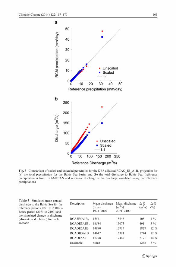
Fig. 3 Comparison of scaled and unscaled percentiles for the DBS adjusted RCAO_E5_A1B3 projection for(a) the total precipitation for the Baltic Sea basin, and (b) the total discharge to Baltic Sea. (referenceprecipitation is from ERAMESAN and reference discharge is the discharge simulated using the referenceprecipitation)

Table 3 Simulated mean annualdischarge to the Baltic Sea for thereference period (1971 to 2000), afuture period (2071 to 2100) andthe simulated change in discharge(absolute and relative) for eachscenario

Description Mean discharge(m3/s)1971–2000

Mean discharge(m3/s)2071–2100

Δ Q(m3/s)

Δ Q(%)

RCA3E5A1B3 15541 15648 108 1 %

RCAOE5A1B3 14584 15075 491 3 %

RCAOE5A1B1 14890 16717 1827 12 %

RCAOH3A1B 14647 16391 1744 12 %

RCAOE5A2 15278 17449 2171 14 %

Ensemble Mean 1268 8 %

Climatic Change (2014) 122:157–170 165

The effect of varying the GCM was, in one case, smaller than the internal variabilitywithin the single GCM, i.e. the RCAOE5A1B1 run showed the same increase to total Q tothe Baltic Sea as the RCAOH3A1B run (Table 3), similar temporal distributions of the futureQ (Fig. 4), but some differences in the spatial distribution of the Q changes (Fig. 5). On theother hand, when comparing the other realisation of the A1B scenario (RCAOE5A1B3) tothe Hadley A1B run, these differences are much larger. Nevertheless internal variabilitywithin GCMs is important to consider.

It is also important to examine internal uncertainties resulting from the hydrologicalimpact modelling chain including the Balt-HYPE model itself and the BC. Even with theBCs made to the precipitation and temperature, biases in the simulated present day Q to theBaltic Sea range from −7 % to +1 % across all scenarios (Table 2). The magnitude of this

Fig. 4 Mean monthly discharge to the Baltic Sea, for period 1 (1971 to 2000) and all projections for period 2(2071 to 2100)

Fig. 5 Mean annual changes to discharge summarised for the 6 main drainage basins of the Baltic Sea

166 Climatic Change (2014) 122:157–170

error is similar to that of the predicted change (e.g. ensemble average 8 %). Although DBSdoes well to adjust the distribution of precipitation events, BC methods generally affect themagnitude of the changes to a variable projected by the raw climate model output and it isdebatable whether this is preferable or not (see Berg et al. 2012; Li et al. 2010). Furthermoreco-variation between variables can be affected and this affects, in particular, the magnitude ofprecipitation stored as snow because it is difficult to correct the timing of temperature eventsaround the melting threshold (Dahné et al. 2013). Finally, the stationarity of the error model forBC is an assumption which warrants further investigation (e.g. Maraun et al. 2010). QuantileBC methods can capture the decadal variability included in the reference (tuning) period, but itis then assumed that the decadal variability outside of this period is sufficiently represented bythe GCM. Other methods (e.g. Dunne et al. 2013) have corrected directly for the magnitude ofdecadal variability, but such methods are still dependent on the length of the reference periodand don’t correct for decadal variations in variable distribution.

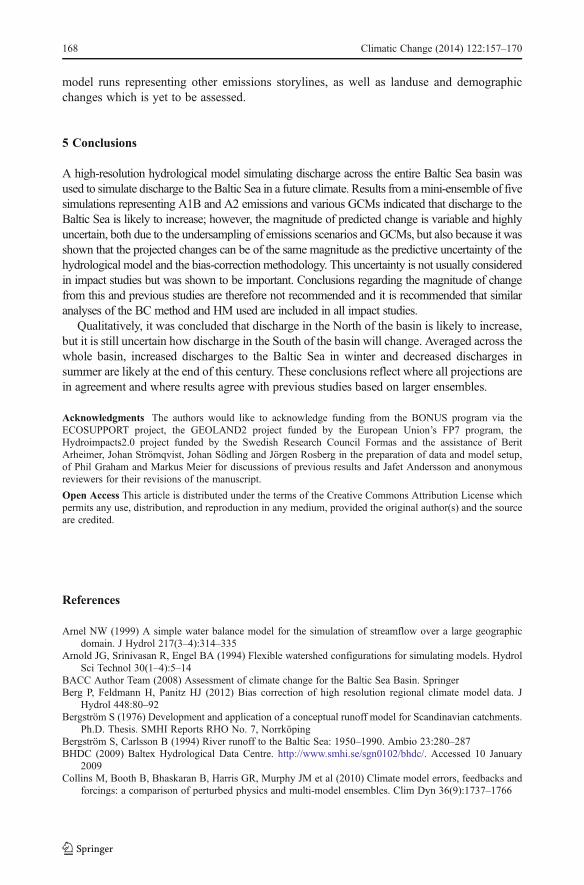
There is also decadal variation in the ability of the Balt-HYPEmodel to correctly simulate Q.A 10-year running mean of volume errors was used to validate whether there were anysignificant temporal deviations in simulated volume to the Baltic Sea over the hindcast period(Fig. 6). The error in simulated volume varied by 9 %: from −7 % (1979–1988) to +2 % (1998to 2007) (validation stations vary for these periods due to data availability). This means that asimulated future change of 8% (the ensemble mean) may simply be a result of the limitations ofthe hydrological model’s response to natural climatic variability, rather than a future climatechange. There are therefore important uncertainties related to the HM used, also indicated byHagemann et al. (2012) using HM ensembles.

Previous studies for the Baltic Sea (e.g. Meier et al. 2006) and other regions (e.g. Olssonet al. 2011; Van Vliet et al. 2012) indicate that they can give a measure of uncertainty simplyby running a large ensemble of GCMs/RCMs. Uncertainties from BC procedures and HMare often ignored or assumed negligible. Until GCMs/RCMs can improve representations ofprecipitation and evapotranspiration, the need to use BC methods and HMs remains. It isstrongly urged that the significant uncertainties due to BC and HMs are further explored andincluded in hydrological impact studies for all regions. Finally, to better predict the realuncertainty for changes in discharge to the Baltic Sea requires a larger ensemble of climate

Fig. 6 Temporal evaluation of model showing running mean volume error for all river mouth stations and themean +/- standard deviation for all river mouths

Climatic Change (2014) 122:157–170 167

model runs representing other emissions storylines, as well as landuse and demographicchanges which is yet to be assessed.

5 Conclusions

A high-resolution hydrological model simulating discharge across the entire Baltic Sea basin wasused to simulate discharge to the Baltic Sea in a future climate. Results from amini-ensemble of fivesimulations representing A1B and A2 emissions and various GCMs indicated that discharge to theBaltic Sea is likely to increase; however, the magnitude of predicted change is variable and highlyuncertain, both due to the undersampling of emissions scenarios and GCMs, but also because it wasshown that the projected changes can be of the same magnitude as the predictive uncertainty of thehydrological model and the bias-correction methodology. This uncertainty is not usually consideredin impact studies but was shown to be important. Conclusions regarding the magnitude of changefrom this and previous studies are therefore not recommended and it is recommended that similaranalyses of the BC method and HM used are included in all impact studies.

Qualitatively, it was concluded that discharge in the North of the basin is likely to increase,but it is still uncertain how discharge in the South of the basin will change. Averaged across thewhole basin, increased discharges to the Baltic Sea in winter and decreased discharges insummer are likely at the end of this century. These conclusions reflect where all projections arein agreement and where results agree with previous studies based on larger ensembles.

Acknowledgments The authors would like to acknowledge funding from the BONUS program via theECOSUPPORT project, the GEOLAND2 project funded by the European Union’s FP7 program, theHydroimpacts2.0 project funded by the Swedish Research Council Formas and the assistance of BeritArheimer, Johan Strömqvist, Johan Södling and Jörgen Rosberg in the preparation of data and model setup,of Phil Graham and Markus Meier for discussions of previous results and Jafet Andersson and anonymousreviewers for their revisions of the manuscript.

Open Access This article is distributed under the terms of the Creative Commons Attribution License whichpermits any use, distribution, and reproduction in any medium, provided the original author(s) and the sourceare credited.

References

Arnel NW (1999) A simple water balance model for the simulation of streamflow over a large geographicdomain. J Hydrol 217(3–4):314–335

Arnold JG, Srinivasan R, Engel BA (1994) Flexible watershed configurations for simulating models. HydrolSci Technol 30(1–4):5–14

BACC Author Team (2008) Assessment of climate change for the Baltic Sea Basin. SpringerBerg P, Feldmann H, Panitz HJ (2012) Bias correction of high resolution regional climate model data. J

Hydrol 448:80–92Bergström S (1976) Development and application of a conceptual runoff model for Scandinavian catchments.

Ph.D. Thesis. SMHI Reports RHO No. 7, NorrköpingBergström S, Carlsson B (1994) River runoff to the Baltic Sea: 1950–1990. Ambio 23:280–287BHDC (2009) Baltex Hydrological Data Centre. http://www.smhi.se/sgn0102/bhdc/. Accessed 10 January

2009Collins M, Booth B, Bhaskaran B, Harris GR, Murphy JM et al (2010) Climate model errors, feedbacks and

forcings: a comparison of perturbed physics and multi-model ensembles. Clim Dyn 36(9):1737–1766

168 Climatic Change (2014) 122:157–170

Dahné J, Donnelly C, Olsson J (2013) Post-processing of climate projections for hydrological impact studies,how well is reference state preserved? Proceedings of IAHS-IAPSO-IASPEI Assembly, Gothenburg,Sweden, July 2013 (IAHS Publ. 2013 in press)

Dunne JP, Stouffer RJ, John JG (2013) Reductions in labour capacity from heat stress under climate warming.Nat Clim Chang 3:563–566

Fowler HJ, Blenkinsop S, Tebaldi C (2007) Linking climate change modelling to impacts studies: recentadvances in downscaling techniques for hydrological modelling. Int J Climatol 27:1547–1578

Gao Y, Vano J, Zhu C, Lettenmaier DP (2011) Evaluating climate change over the Colorado River basin usingregional climate models. J Geophys Res 116, D13104. doi:10.1029/2010JD015278

GLC (2009) Global Landcover 2000. http://ies.jrc.ec.europa.eu/global-land-cover-2000 Accessed 10 January2009

Graham LP (2004) Climate change effects on river flow to the Baltic Sea. Ambio 33(4–5):235–241Graham LP, Hagemann S, Jaun S, Beniston M (2007) On interpreting hydrological change from regional

climate models. Clim Chang 81:97–122GRDC (2009). Global Runoff Data Center http://www.bafg.de/GRDC/EN/Home/homepage__node.html

Accessed 10 January 2009Hagemann S, Dumenil L (1999) Application of a global discharge model to atmospheric model simulations in

the BALTEX region. Nord Hydrol 30:209–230Hagemann S, Göttel H, Jacob D, Lorenz P, Roeckner E (2009) Improved regional scale processes in projected

hydrological changes over large European catchments. Clim Dyn 32:767–781Hagemann S et al (2012) Climate change impact on available water resources obtained using multiple global

climate and hydrology models. Earth Syst Dynam Discuss 3:1321–1345, www.earth-syst-dynam-discuss.net/3/1321/2012/

Hansson D, Eriksson C, Omstedt A, Chen D (2011) Reconstruction of river runoff to the Baltic Sea, AD1500–1995. Int J Climatol 31:696–703

Hay LE, McCabe GJ (2010) Hydrologic effects of climate change on the Yukon River Basin. Clim Chang100(3-4):509–523

Hurkmans RTWL, Terink W, Uijlenhoet R, Torfs PJJF, Jacob D, Troch PA (2010) Changes in streamflow dynamicsin the Rhine basin under three high-resolution climate scenarios. J Clim 23:679–699

IPCC (2001) Climate Change 2001: impacts, adaptation and vulnerability. Contribution of Working Group IIto the Third Assessment Report of the Intergovernmental Panel on Climate Change. CambridgeUniversity Press, Cambridge New York

Jansson A, Persson C, Strandberg G (2007) 2D meso-scale re-analysis of precipitation, temperature and windover Europe – ERAMESAN Time period 1980–2004. SMHI Reports: Meteorology and climatology no.112, SMHI, Norrköping

JRC (2006) European Soils Database. http://eusoils.jrc.ec.europa.eu/ESDB_Archive/ESDB/index.htm. Accessed5 February 2009

Jungclaus JH, Botzet M, Haak H, Keenlyside N, Luo J-J et al (2006) Ocean circulation and tropical variabilityin the coupled ECHAM5/MPI-OM. J Clim 19:3952–3972

Kjellström E, Nikolin G, Hansson U, Strandberg G, Ullerstig A (2010) 21st century changes in the Europeanclimate: uncertainties derived from an ensemble of regional climate model simulations. Tellus 63A(1):24–40. doi:10.1111/j.1600-0870.2010.00475

Kling H, Fuchs M, Paulin M (2012) Runoff conditions in the upper Danube basin under an ensemble ofclimate change scenarios. J Hydrol 424–425:264–277

Li H, Sheffield J, Wood EF (2010) Bias correction of monthly precipitation and temperature fields fromIntergovernmental Panel on Climate Change AR4 models using equidistant quantile matching. J GeophysRes 115, D10101. doi:10.1029/2009JD012882

Liang X, Lettenmaier DP, Wood EF, Burges J (1994) A simple hydrologically based model of land surfacewater and energy fluxes for GSMs. J Geophys Res 99(D7):14415–14428

Lindström G, Pers CP, Rosberg R, Strömqvist J, Arheimer B (2010) Development and test of the HYPE(Hydrological Predictions for the Environment) model – Awater quality model for different spatial scales.Hydrol Res 41:295–319

Maraun D et al (2010) Precipitation downscaling under climate change: Recent developments to bridge thegap between dynamical models and the end user. Rev Geophys 48. RG3003

Meier HEM, Kjellström E, Graham LP (2006) Estimating uncertainties of projected Baltic Sea salinity in thelate 21st century. Geophys Res Lett 33:4pp. doi:10.1029/2006gl026488

Meier HEM, Höglund A, Döscher R, Andersson H, Löptien U, Kjellström E (2011) Quality assessment ofatmospheric surface fields over the Baltic Sea of an ensemble of regional climate model simulations withrespect to ocean dynamics. Oceanologia 53:193–227

Climatic Change (2014) 122:157–170 169

Meleshko VP, Kattsov VM, Govorkova VA, Malevsky-Malevich SP, Nadezhina ED, Sporyshev PV (2004)Anthropogenic climate changes in Northern Eurasia in the 21st century. Russ Meteorol Hydrol 7:5–26

Nakicenovic N, Swart R (eds) (2000) Special report on emissions scenarios. In A Special Report of WorkingGroup III of the Intergovernmental Panel on Climate Change. Cambridge University Press, Cambridge,United Kingdom and New York, NY, USA, 599

Olsson J, Yang W, Graham LP, Rosberg J, Andréasson J (2011) Using an ensemble of climate projections forsimulating recent and near-future hydrological change to lake Vänern in Sweden. Tellus A 63:126–137

Omstedt A et al (2012) Future changes of the Baltic Sea acid-base (pH) and oxygen balances. Tellus B64:19586

Piani C, Haerter JO, Coppola E (2010) Statistical bias correction for daily precipitation in regional climatemodels over Europe. Theor Appl Climatol 99(1–2):187–192

Strömqvist J, Arheimer B, Dahné J, Donnelly C, Lindström G (2012) Water and nutrient predictions inungauged basins – Set-up and evaluation of a model at the national scale. Hydrol Sci J 57(2):229–247

Themeßl MJ, Gobiet A, Leuprecht A (2010) Empirical-statistical downscaling and error correction of dailyprecipitation from regional climate models. Int J Climatol 31(10):1530–1544

USGS (2000) Hydro1k Elevation Derivative Database. http://edc.usgs.gov/products/elevation/gtopo30/hydro/index.html . Accessed 16 February 2009.

Van Vliet MTH, Yearsley JR, Ludwig F, Vögele S, Lettenmaier DP, Kabat P (2012) Vulnerability of U.S. andEuropean electricity supply to climate change. Nat Clim Chang 2(9):676–681

Vörösmarty CJB et al (1989) Continental scale models of water balance and fluvial transport: an application toSouth America, Global Biogeochem. Cycles 3(3):241–265

Yang W, Andreásson J, Graham LP, Olsson J, Rosberg J, Wetterhall F (2010) Distribution-based scaling toimprove usability of regional climate model projections for hydrological climate change impacts studies.Hydrol Res 41(3–4):211–228

170 Climatic Change (2014) 122:157–170