River Influences on Shelf Ecosystems: Introduction and

River Influences on Shelf Ecosystems: Introduction and synthesis

B. M. Hickey,1 R. M. Kudela,2 J. D. Nash,3 K. W. Bruland,2 W. T. Peterson,4

P. MacCready,1 E. J. Lessard,1 D. A. Jay,5 N. S. Banas,6 A. M. Baptista,7 E. P. Dever,3

P. M. Kosro,3 L. K. Kilcher,3 A. R. Horner-Devine,8 E. D. Zaron,5 R. M. McCabe,9

J. O. Peterson,3 P. M. Orton,10 J. Pan,5 and M. C. Lohan11

Received 21 April 2009; revised 23 July 2009; accepted 26 August 2009; published 3 February 2010.

[1] River Influences on Shelf Ecosystems (RISE) is the first comprehensiveinterdisciplinary study of the rates and dynamics governing the mixing of river and coastalwaters in an eastern boundary current system, as well as the effects of the resultant plumeon phytoplankton standing stocks, growth and grazing rates, and community structure.The RISE Special Volume presents results deduced from four field studies and twodifferent numerical model applications, including an ecosystem model, on the buoyantplume originating from the Columbia River. This introductory paper provides backgroundinformation on variability during RISE field efforts as well as a synthesis of results, withparticular attention to the questions and hypotheses that motivated this research. RISEstudies have shown that the maximum mixing of Columbia River and ocean water occursprimarily near plume liftoff inside the estuary and in the near field of the plume. Mostplume nitrate originates from upwelled shelf water, and plume phytoplankton species aretypically the same as those found in the adjacent coastal ocean. River-supplied nitratecan help maintain the ecosystem during periods of delayed upwelling. The plume inhibitsiron limitation, but nitrate limitation is observed in aging plumes. The plume also hassignificant effects on rates of primary productivity and growth (higher in new plumewater) and microzooplankton grazing (lower in the plume near field and north of theriver mouth); macrozooplankton concentration (enhanced at plume fronts); offshelfchlorophyll export; as well as the development of a chlorophyll ‘‘shadow zone’’ offnorthern Oregon.

Citation: Hickey, B. M., et al. (2010), River Influences on Shelf Ecosystems: Introduction and synthesis, J. Geophys. Res., 115,

C00B17, doi:10.1029/2009JC005452.

1. Introduction: RISE Hypotheses

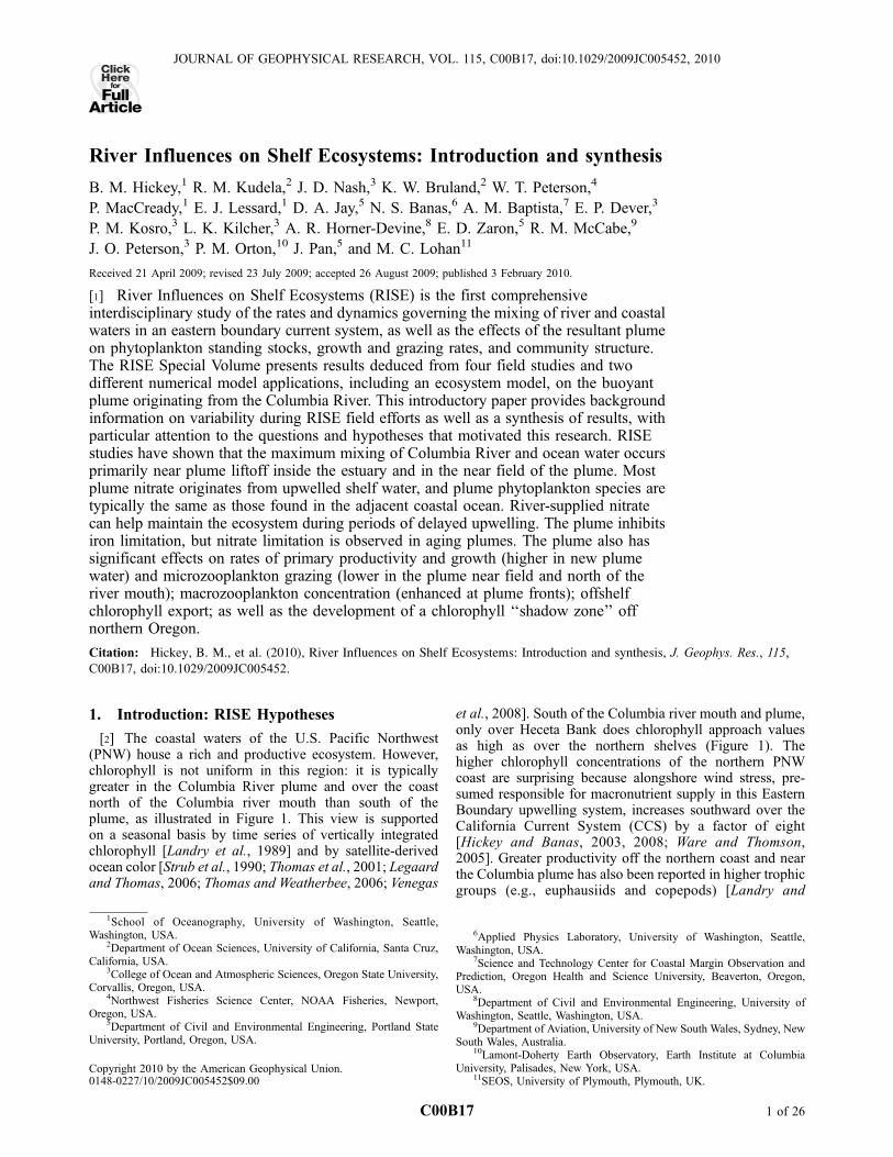
[2] The coastal waters of the U.S. Pacific Northwest(PNW) house a rich and productive ecosystem. However,chlorophyll is not uniform in this region: it is typicallygreater in the Columbia River plume and over the coastnorth of the Columbia river mouth than south of theplume, as illustrated in Figure 1. This view is supportedon a seasonal basis by time series of vertically integratedchlorophyll [Landry et al., 1989] and by satellite-derivedocean color [Strub et al., 1990; Thomas et al., 2001; Legaardand Thomas, 2006; Thomas and Weatherbee, 2006; Venegas

et al., 2008]. South of the Columbia river mouth and plume,only over Heceta Bank does chlorophyll approach valuesas high as over the northern shelves (Figure 1). Thehigher chlorophyll concentrations of the northern PNWcoast are surprising because alongshore wind stress, pre-sumed responsible for macronutrient supply in this EasternBoundary upwelling system, increases southward over theCalifornia Current System (CCS) by a factor of eight[Hickey and Banas, 2003, 2008; Ware and Thomson,2005]. Greater productivity off the northern coast and nearthe Columbia plume has also been reported in higher trophicgroups (e.g., euphausiids and copepods) [Landry and

1School of Oceanography, University of Washington, Seattle,Washington, USA.

2Department of Ocean Sciences, University of California, Santa Cruz,California, USA.

3College of Ocean and Atmospheric Sciences, Oregon State University,Corvallis, Oregon, USA.

4Northwest Fisheries Science Center, NOAA Fisheries, Newport,Oregon, USA.

5Department of Civil and Environmental Engineering, Portland StateUniversity, Portland, Oregon, USA.

Copyright 2010 by the American Geophysical Union.0148-0227/10/2009JC005452$09.00

6Applied Physics Laboratory, University of Washington, Seattle,Washington, USA.

7Science and Technology Center for Coastal Margin Observation andPrediction, Oregon Health and Science University, Beaverton, Oregon,USA.

8Department of Civil and Environmental Engineering, University ofWashington, Seattle, Washington, USA.

9Department of Aviation, University of New South Wales, Sydney, NewSouth Wales, Australia.

10Lamont-Doherty Earth Observatory, Earth Institute at ColumbiaUniversity, Palisades, New York, USA.

11SEOS, University of Plymouth, Plymouth, UK.

JOURNAL OF GEOPHYSICAL RESEARCH, VOL. 115, C00B17, doi:10.1029/2009JC005452, 2010ClickHere

for

FullArticle

C00B17 1 of 26

http://dx.doi.org/10.1029/2009JC005452

Lorenzen, 1989]. In spring and summer, juvenile salmonare more abundant on the shelf north of the river mouth[Pearcy, 1992; Bi et al., 2007; J. O. Peterson, unpublisheddata, 2009].[3] In 2004 an interdisciplinary study ‘‘River Influences

on Shelf Ecosystems’’ (RISE) was initiated to determine theextent to which alongshore gradients in ecosystem produc-tivity might be related to the existence of the massivefreshwater plume from the Columbia River. RISE wasdesigned to test three hypotheses: (1) During upwellingthe growth rate of phytoplankton within the Columbiaplume exceeds that in nearby areas outside the plume beingfueled by the same upwelling nitrate. (2) The plumeenhances cross-margin transport of plankton and nutrients.(3) Plume-specific nutrients (Fe and Si) alter and enhanceshelf productivity preferentially north of the river mouth.[4] RISE is the first comprehensive interdisciplinary

study of the rates and dynamics governing the mixing ofriver and coastal waters in an eastern boundary system, aswell as the effects of the buoyant plume formed by thoseprocesses on phytoplankton growth and grazing rates,

standing stocks and community structure in the localecosystem. This paper presents an overview of the projectmeasurements and setting as well as a synthetic view ofresults. Background information on shelf processes, theColumbia River estuary and the Columbia River plume ispresented in section 2, followed by a description of theRISE sampling scheme and numerical models (section 3).The environmental and biological setting of the RISE studyyears is given in section 4. Study results as they pertain toplume-related questions and hypotheses are discussed insection 5 and summarized in section 6.

2. Background

2.1. Shelf Processes Influencing the Columbia Plume

[5] The buoyant plume from the Columbia River islocated near the northern terminus of an eastern boundarycurrent. Water property, nutrients, biomass and currentvariability are governed by wind-driven processes anddominated by the seasonal cycle. The seasonal variabilityof physical, chemical and biological properties for both

Figure 1. (left) Satellite-derived chlorophyll data (23 July 2004) illustrating the typically observedhigher chlorophyll in the Columbia plume as well as north of the river mouth (compared to south ofthe plume). The image was obtained under strong upwelling conditions, with a well-developed southwesttending plume as well as remnants of a north tending plume [Liu et al., 2009a]. Alongshore chlorophyllpatterns agree well with observations presented later in the paper (Figure 7a). (right) Satellite-derivedchlorophyll and turbidity 12 June 2005 illustrating a well-developed southwest tending Columbia plumeand a weaker north tending plume. The image was obtained one day after model runs shown in Figure 10.Data acquired from Kudela Laboratory.

C00B17 HICKEY ET AL.: RISE INTRODUCTION AND SYNTHESIS

2 of 26

C00B17

Oregon and Washington are documented in Landry et al.[1989] and in the book edited by Landry and Hickey [1989].In winter, large-scale currents are primarily northward (theDavidson Current); in summer, large-scale currents areprimarily southward (the California Current) [Hickey,1979, 1989, 1998]. A coast-wide phenomenon that initiatesthe uplift of isopycnals and associated higher nutrient andlower oxygen water from the continental slope to the shelf,the ‘‘Spring Transition’’ [Huyer et al., 1979; Strub et al.,1987], separates winter from the springtime growing sea-son. Both the spring transition and the seasonal continuationof upwelling through the fall season have been attributed inpart to winds south of the region (i.e., ‘‘remote forcing’’)[Strub et al., 1987; Hickey et al., 2006; Pierce et al., 2006].The uplifted isopycnals result in the formation of a south-ward baroclinic coastal jet, a feature which in mid summeris generally concentrated over the outer shelf and upperslope off the coasts of northern Oregon [Kosro, 2005] andWashington [MacFadyen et al., 2005].[6] Fluctuations in currents and water properties in this

region occur on scales of 2–20 days throughout the year[Hickey, 1989]. These fluctuations are driven in part byfluctuations in local winds, and in part by coastally trappedwaves generated by remote winds [Battisti and Hickey,1984]. Although, a change in wind direction from upwellingfavorable (southward) to downwelling favorable (north-ward) reverses the direction of flow from southward tonorthward on the inner shelf where flow is frictionallydominated [Hickey et al., 2005], surface currents on theouter shelf and slope rarely reverse [Kosro, 2005;MacFadyen et al., 2008]. The stability of the shelf breakjet is due primarily to its baroclinic nature: reversals of windstress to downwelling favorable are insufficient to com-pletely erode the seasonally uplifted isopycnals during theupwelling season. However, within a distance of about10 km from the coast (the scale of the internal Rossbyradius of deformation), the response to changes in winddirection is almost immediate (�3 h) [Hickey, 1989],resulting in significant vertical movement of isopycnals ontime scales of a few days. When winds are directedsouthward, the associated upwelling of nutrient-rich wateron the inner shelf fuels coastal productivity, resulting inchanges in chlorophyll concentration that follow thechanges in wind direction. During an upwelling event,phytoplankton begin to grow as a response to the infusionof nutrients near the coast and this ‘‘bloom’’ is advectedoffshore, continuing to grow while depleting the nutrientsupply. When winds relax or reverse, the bloom moves backtoward shore where it can contact the coast and even entercoastal estuaries [Roegner et al., 2002].[7] Although alongshelf currents do not typically reverse

on the mid to outer shelf, currents in the surface Ekmanlayer frequently reverse from onshore to offshore and viceversa in response to southward or northward wind stress,respectively [Hickey et al., 2005]. Cross-shelf movement ofbuoyant plumes is particularly sensitive to wind stressdirection, because the Ekman layer is compressed by theplume stratification so that velocities are correspondinglyhigher [Garcia-Berdeal et al., 2002].[8] Water flowing south toward the Columbia plume

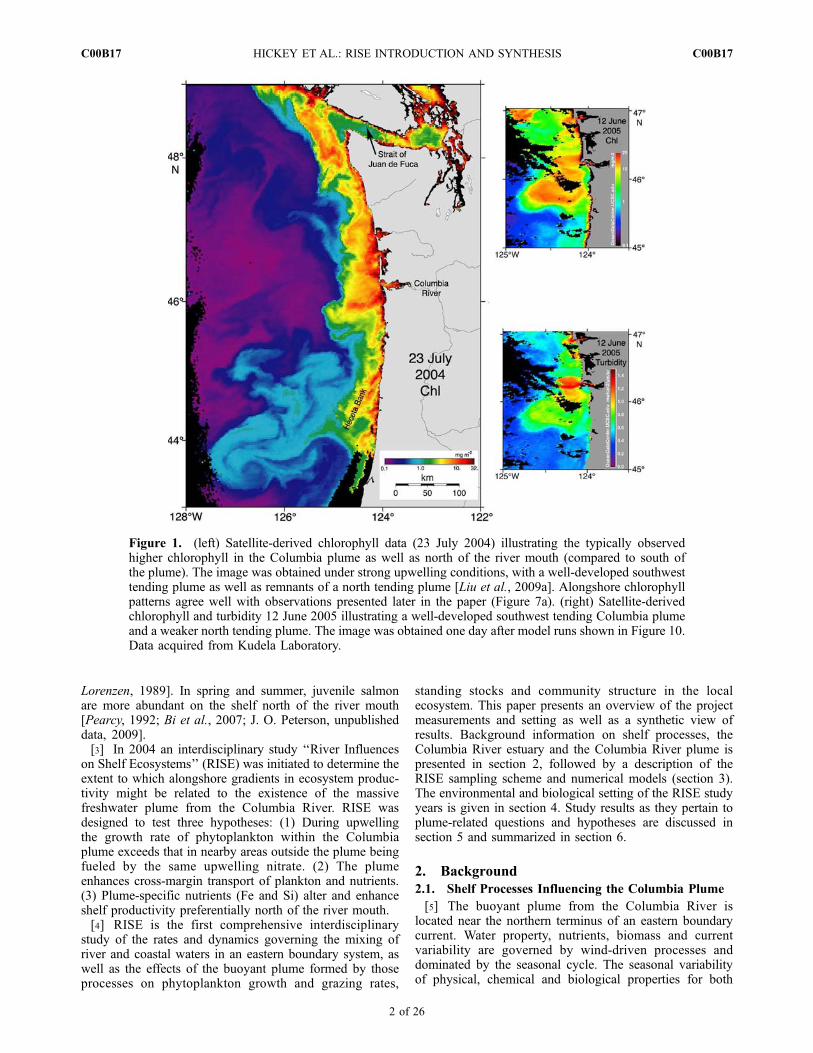
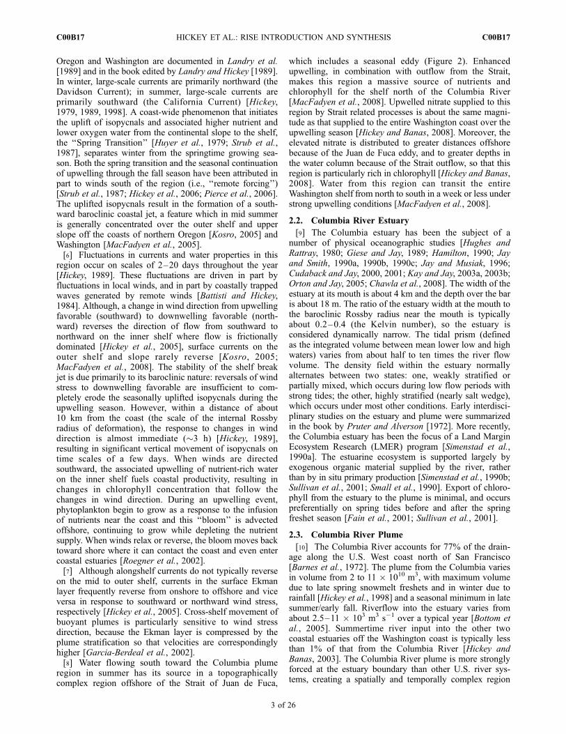
region in summer has its source in a topographicallycomplex region offshore of the Strait of Juan de Fuca,

which includes a seasonal eddy (Figure 2). Enhancedupwelling, in combination with outflow from the Strait,makes this region a massive source of nutrients andchlorophyll for the shelf north of the Columbia River[MacFadyen et al., 2008]. Upwelled nitrate supplied to thisregion by Strait related processes is about the same magni-tude as that supplied to the entire Washington coast over theupwelling season [Hickey and Banas, 2008]. Moreover, theelevated nitrate is distributed to greater distances offshorebecause of the Juan de Fuca eddy, and to greater depths inthe water column because of the Strait outflow, so that thisregion is particularly rich in chlorophyll [Hickey and Banas,2008]. Water from this region can transit the entireWashington shelf from north to south in a week or less understrong upwelling conditions [MacFadyen et al., 2008].

2.2. Columbia River Estuary

[9] The Columbia estuary has been the subject of anumber of physical oceanographic studies [Hughes andRattray, 1980; Giese and Jay, 1989; Hamilton, 1990; Jayand Smith, 1990a, 1990b, 1990c; Jay and Musiak, 1996;Cudaback and Jay, 2000, 2001; Kay and Jay, 2003a, 2003b;Orton and Jay, 2005; Chawla et al., 2008]. The width of theestuary at its mouth is about 4 km and the depth over the baris about 18 m. The ratio of the estuary width at the mouth tothe baroclinic Rossby radius near the mouth is typicallyabout 0.2–0.4 (the Kelvin number), so the estuary isconsidered dynamically narrow. The tidal prism (definedas the integrated volume between mean lower low and highwaters) varies from about half to ten times the river flowvolume. The density field within the estuary normallyalternates between two states: one, weakly stratified orpartially mixed, which occurs during low flow periods withstrong tides; the other, highly stratified (nearly salt wedge),which occurs under most other conditions. Early interdisci-plinary studies on the estuary and plume were summarizedin the book by Pruter and Alverson [1972]. More recently,the Columbia estuary has been the focus of a Land MarginEcosystem Research (LMER) program [Simenstad et al.,1990a]. The estuarine ecosystem is supported largely byexogenous organic material supplied by the river, ratherthan by in situ primary production [Simenstad et al., 1990b;Sullivan et al., 2001; Small et al., 1990]. Export of chloro-phyll from the estuary to the plume is minimal, and occurspreferentially on spring tides before and after the springfreshet season [Fain et al., 2001; Sullivan et al., 2001].

2.3. Columbia River Plume

[10] The Columbia River accounts for 77% of the drain-age along the U.S. West coast north of San Francisco[Barnes et al., 1972]. The plume from the Columbia variesin volume from 2 to 11 � 1010 m3, with maximum volumedue to late spring snowmelt freshets and in winter due torainfall [Hickey et al., 1998] and a seasonal minimum in latesummer/early fall. Riverflow into the estuary varies fromabout 2.5–11 � 103 m3 s�1 over a typical year [Bottom etal., 2005]. Summertime river input into the other twocoastal estuaries off the Washington coast is typically lessthan 1% of that from the Columbia River [Hickey andBanas, 2003]. The Columbia River plume is more stronglyforced at the estuary boundary than other U.S. river sys-tems, creating a spatially and temporally complex region


3 of 26

C00B17

near the river mouth. Because of the narrow outlet to theocean, strong tidal currents and significant freshwater flow,surface currents in the tidal plume often exceed 3 m s�1

during strong ebb tides. As a result the Columbia Riverproduces a highly supercritical outflow that propagatesseaward as a gravity current during each ebb tide. Theleading edge front, termed the ‘‘tidal plume front,’’ produ-ces strong horizontal convergences, vertical velocities andmixing [Orton and Jay, 2005; Morgan et al., 2005].

[11] The historical picture of the Columbia River plumedepicts a low salinity feature oriented southwest offshore ofthe Oregon shelf in summer (e.g., Figure 1) and north ornorthwest along the Washington shelf in winter [Barnes etal., 1972; Landry et al., 1989]. The RISE hypotheses werebased on that view of the Columbia. Recently, Hickey et al.[2005] have demonstrated that the plume can be presentmore than a hundred kilometers north of the river mouth onthe Washington shelf from spring to fall. This study showedthat the plume is frequently bidirectional, with simultaneous

Figure 2. Locations of all sampling transects, moored sensor arrays and wind buoys, and CODARranges plotted on a satellite-derived sea surface temperature image on 21 June 2006. Regional physicalfeatures of interest are noted.


4 of 26

C00B17

branches both north and south of the river mouth. Thisspatial structure was subsequently confirmed by remotesensing [Thomas andWeatherbee, 2006].Duringdownwellingfavorable winds, the southwest plume moves onshore overthe Oregon shelf. At the same time, a new plume formsnorth of the river mouth, trapped within �20–30 km ofthe coast. This plume propagates and also is advectednorthward by inner shelf currents that reverse during thedownwelling winds. When winds return to upwellingfavorable, inner shelf currents reverse immediately tosouthward and the shallow plume is advected offshore inthe wind-driven Ekman layer to the central shelf, andsouthward in the seasonal mean ambient flow [Hickey etal., 2005]. The possibility of a bidirectional Columbiaplume depends critically on the existence of mean ambientflow in the direction opposite to its rotational tendency.Because three out of four RISE cruises occurred early inthe upwelling season, most sampling took place in abidirectional plume environment.[12] On subtidal time scales, numerical and laboratory

models of river plume formation in a rotating system underconditions of no applied winds and no ambient flowdemonstrate that a plume forms a non linear ‘‘bulge region’’and a quasi-geostrophic ‘‘coastal current’’ downstream ofthe bulge [e.g., Chao and Boicourt, 1986; Garvine, 1999;Yankovsky et al., 2001; Fong and Geyer, 2002; Horner-Devine et al., 2006]. These prior studies addressed thedynamics of unidirectional plumes for conditions mosttypical of the U.S. east coast: shallow broad shelves andmodest riverflow and ambient flow (if included) in thedirection of plume formation. However, the Columbia Rivergenerates a large volume plume which emerges onto arelatively narrow continental shelf. Perhaps its most unusualcharacteristic is that in summer it usually encounters ambi-ent flow moving counter to the rotational tendency of theplume. Prior to RISE, only the model study by Garcia-Berdeal et al. [2002] directly addressed conditions applica-ble to the Columbia. That study provided a dynamical basisfor the existence of a bidirectional plume and the timevarying response of the plume to variable winds as well asto ambient flow both in the same direction as, and counterto, the rotational tendency. The study also demonstrated thatover the shelf away from the river mouth, the effect of theplume on the velocity field is confined to layers of lowsalinity (i.e., the plume effect is baroclinic), as shown in awintertime Columbia plume data set [Hickey et al., 1998].[13] With respect to nutrients, historical studies showed

that in summer the Columbia plume usually suppliesexceptionally high concentrations of silicic acid but verylittle nitrate, to the plume region [Conomos et al., 1972].Because sediment transport and deposition from the Co-lumbia plume is highest north of the river mouth[Nittrouer, 1978], that shelf potentially has a massive supplyof Fe-rich sediment deposited on the mid shelf region readyto be delivered to the euphotic zone by upwelling of bottomwater that has been in contact with the sediments. Inaddition, the broader, flatter shelf north of the river mouthhas been hypothesized to provide opportunity for increasedduration of bottom contact (hence access to Fe) of upwell-ing waters than the narrower, steeper shelf to the south[Bruland et al., 2001; Chase et al., 2007]. The midshelfmud deposits can be thought to act like an iron capacitor;

charging in the winter with the higher sediment transportassociated with winter flood events, and discharging duringthe summer upwelling periods.

3. RISE Sampling Scheme and Modeling Systems

[14] The overall RISE sampling strategy was to comparemixing rates, nutrient supply, and phytoplankton produc-tion, grazing and community structure within the plume andoutside the plume; i.e., on the shelf north of the river mouth,presumed more productive, and on the shelf south of theriver mouth, presumed less productive, as well as in theimportant ‘‘plume liftoff’’ zone (the region where the plumeloses contact with the bottom, located in the river entranceto �5 km offshore of the entrance jetties). The backbone forthis project consists of data collected during four cruisesthat took place in the seasonally high flow period (May–June) in each of three years (2004–2006) and in a low flowperiod in one year (August 2005). The sampling was spreadover three years to include potential interannual differencesin processes related to wind and river flow variability. The21 day length of the cruises ensured that a variety of circulationand growth regimes, including upwelling, relaxation,downwelling, and neap/spring tides were observed. A listof program elements including data collected, models andtechniques as well as team leaders is given in Table 1.[15] The sampling plan as originally proposed was based

on the historical picture of a primarily southwest tendingColumbia plume. However, due to the rarity of persistentupwelling favorable winds on RISE cruises, southwesttending plumes were the exception rather than the rule. Inparticular, on two of the cruises, June 2005 and May–June2006, north tending plumes were dominant: RISE samplingwas adapted to this situation, and samples were obtainedalong the Washington coast as far north as the Strait of Juande Fuca in 2006.[16] The field studies used two vessels operating simul-

taneously. The R/V Wecoma obtained primarily biologicaland chemical rate data: (1) at individual stations on cardinaltransects north and south of the river mouth (Grays Harborand Cape Meares; see Figure 2) and near the river mouth;(2) at selected process study stations; and (3) at fixedstations near the river mouth during strong neap and springtides (time series). A towed sensor package was used toobtain micronutrient samples near the sea surface on cardi-nal transects and selected other transects. Underway mea-surements included macronutrients (N, P, Si), dissolvedtrace metals (Fe, Mn), supplemented with discrete samplesfrom the underway system (microscopy, FlowCAM andparticulate trace metals) as well as ADCP (75 kHz) measure-ments of velocity. At CTD stations vertical profiles (0–200mwhere possible; and 500 m at selected stations) of T, S,currents, dissolved O2, in vivo fluorescence, transmissivity,PAR, and bottle samples for chlorophyll a, dissolved macro-nutrients (NO3, NH4, urea, PO4, SiO4), dissolved tracemetals, and heterotrophic and autotrophic plankton compo-sition were obtained. In addition, primary production meas-urements were made each day at noon, and phytoplanktongrowth and microzooplankton grazing measurementswere made every one to two days. Macrozooplanktonwere sampled with vertically towed nets and obliquelytowed Bongo nets at selected stations; macrozooplankton


5 of 26

C00B17

experimental work included egg production rates ofcopepods and euphausiids and molting rates of euphausiids,to obtain estimates of secondary production. Surfacedrifters were used to follow the mixing of individual plumesfrom the Columbia and to provide information on surfacecurrents.[17] On the R/V Point Sur, synoptic mesoscale and fine-

scale features were sampled with underway measurementsof near-surface T, S, velocity, particle size and concentra-tion, PAR, transmissivity, fluorescence, and nitrate + nitrite.The Point Sur’s Triaxus tow fish provided high-resolutionsections of T, S, zooplankton (Laser-OPC), PAR andtransmissivity, fluorescence, particle size and concentration(LISST-100), UV absorption and nitrate (Satlantic ISUS),upward-looking ADCP velocity (1200 kHz), and radiance/irradiance (7 channels) through the upper water column to30–35 m. Rapidly executed transects of turbulence and finestructure were also carried out using the Chameleon profiler;these provide full depth profiles of T, S, optics (880 nmbackscatter and fluorescence), turbulence dissipation ratesand fluxes every 1–3 min. During selected periods, transects(primarily those identified in Figure 2) were repeated hourlyto capture the high-frequency evolution in the plume’s near-field and river estuary. Over-the-side deployed acoustics(1200 kHz ADCP and 120 kHz echosounder; 1 m nominaldepth) augmented the hull-mounted 75 and 300 kHz units toimage fine-scale features of the velocity and backscatterfields, resolving fronts, nonlinear internal waves, and tur-bulent billows.[18] The temporal context for observed variability was

provided by an array of moored sensors deployed in theplume near field as well as on the shelf north and south ofthe plume (Figure 2), complemented by the preexistinglong-term estuarine and plume stations of the CORIE/

SATURN network [Baptista, 2006]. To better resolveregional differences, RISE moorings were moved farthernorth and south to the cardinal sampling transects after thefirst year of the program (Figure 2). Surface currents weremapped hourly from shore using HF radar with twosimultaneously operating arrays, one with a 40 km rangeand a 2 km range resolution, the other with a 150 km rangeand a 6 km range resolution. Satellite ocean color, seasurface temperature, turbidity and synthetic aperture radar(SAR) were also obtained when available.[19] Two modeling systems were developed or enhanced

during RISE. The system developed specifically for RISEemployed a structured grid model (the Regional OceanModeling System (ROMS)) and was used in hindcast mode[MacCready et al., 2009]. The CORIE/SATURN modelingsystem [Baptista, 2006], based on two unstructured gridmodels (SELFE, Zhang and Baptista [2008]; ELCIRC, Zhanget al. [2004]), was used in both near real-time prognostic mode(http://www.stccmop.org/datamart/forecasts/simpletool) andmultiyear hindcast mode [e.g., Burla et al., 2009]. Bothmodeling systems incorporated the estuary in the simulationdomain (although at different resolutions) and used realisticatmospheric, river and ocean forcing including tides. Wind/heat flux model forcing for ROMS was derived from the4 km MM5 regional wind/heat flux model [Mass et al.,2003]. SELFE and ELCIRC were also forced by MM5.Conditions on open boundaries were provided by NavalResearch Laboratory (NRL) models; ROMS used the smallerdomain, higher-resolution (�9 km)NCOM-CCSNRLmodel[Shulman et al., 2004], SELFE and ELCIRC used the largerdomain, lower-resolution (�16 km) global NCOM model[Barron et al., 2006]. These models have proven moreeffective in this region than climatology because theyassimilate satellite altimetry and sea surface temperature,

Table 1. RISE Program Elements

Component Techniques Team Leaders

Management and Synthesis HickeyPhysical Modeling Numerical models, ROMS and SELFE with MM5 forcing,

NCOM boundaries, tidesMacCready, Baptista

Biophysical Modeling 3D Numerical models BanasWater Properties, Underway and CTD Underway and CTD Hickey, Jay, KudelaWater Properties TRIAXUS tow-fish JayWater Properties Moored arrays DeverSuspended Particulates,Concentration and Size

LISST-FLOC, acoustic backscatter Jay, Horner-Devine

Chlorophyll a and Phaeopigments In vivo and in vitro fluorometry KudelaDissolved Nutrients including Trace Metals Surveys and towed fish, Lachat autoanalyzer flow injection,

voltammetry, extraction/ICP-MSBruland, Kudela

Picoplankton Flow cytometry KudelaAutotrophic/Heterotrophic Pico-, Nano-,Microplankton Abundance/Taxa

Epifluorescence and light microscopy Lessard

Nitrogen Uptake 15N nitrogen kinetics KudelaPhytoplankton Growthand Microzooplankton Grazing Rates

Dilution method – size-fractionated chlorophyll a, microscopy Lessard

Primary Production 14C uptake KudelaMacrozooplankton Species and Abundance,Growth, Egg Production

Net tows, Laser Optical Plankton Counter (LOPC), microscopy Peterson

Hydrology USGS data JayWater Column Currents Moorings, ADCP surveys Dever, JayMixing Rates, Vertical Fluxes Profiles Nash, MoumSurface Eulerian Currents CODAR, up to 180 km KosroSurface Lagrangian Currents GPS drifters (with C, T) HickeyRemote Sensing of Sea Surface Temperature,Color and Fluorescence

AVHRR, SeaWiFS, MODIS, Bio-Optical modeling Kudela

Plume Position, Fronts, and Internal Waves Synthetic Aperture Radar (SAR) Jay


6 of 26

C00B17

thus ensuring the reasonable development of a southwardcoastal jet, as well as inclusion of low mode coastal trappedwaves that are a significant part of the subtidal scale varianceat midshelf in this region [Battisti and Hickey, 1984]. Bothmodels became integral tools for planning and/or analysiswithin RISE.[20] The ROMS model was also used for biologically

motivated particle-tracking studies [Banas et al., 2009a] andecosystem modeling [Banas et al., 2009b]. The biologicalmodel is a four-box (‘‘NPZD’’) nitrogen budget model thattracks nutrients, phytoplankton, microzooplankton, anddetritus in every cell of the ROMS grid. The rich RISEbiological data set allowed direct model validation againstnot just stocks (chlorophyll, microzooplankton, nutrients)but rates (phytoplankton growth and microzooplanktongrazing), a level of validation that is seldom possible.Rate observations also allowed key model parameters(e.g., microzooplankton ingestion rate and mortality) to beprescribed empirically [Banas et al., 2009b].[21] During the RISE field years, another interdisciplinary

program took place along the central to northernWashington, southern British Columbia coast. This project(Ecology of Harmful Algal Blooms Pacific Northwest,ECOHAB PNW), with a scientific team and suite ofmeasurements similar to that of RISE, focused on thedevelopment of blooms of toxigenic Pseudo-nitzschia inthe Juan de Fuca eddy region (see Figure 2) and theirsubsequent transport to the Washington coast. Surveyswere made as far south as offshore of Willapa Bay, and as

far north as central Vancouver Island. Both RISE andECOHAB PNW sampled a line off Grays Harbor, and thecombined survey data were used in several papers in this andprevious volumes [Hickey et al., 2006; Kudela et al., 2006;Frame and Lessard, 2009]. Data from the moored arrays inthe two programs (see locations in Figure 2) have also beenused together in papers for this volume [Hickey et al., 2009].

4. The RISE Years: Environmental and BiologicalSetting

[22] Time series of the two commonly used indices forinterannual variability, the Multivariate El Nino/SouthernOscillation Index (MEI) and the Pacific Decadal Oscillation(PDO) illustrate that RISE studies all took place withinperiods when both indices were generally positive (Figure 3).Columbia and Willamette River (a major lower basinColumbia River tributary) flows are lowest in years whenthe PDO is positive (with a warm coastal ocean in thePacific Northwest) and the MEI index is positive (indicatingEl Nino-like conditions). Average flows are about 20%lower than in La Nina years when the PDO is negative[Dracup and Kahya, 1994; Gershunov et al., 1999; Bottomet al., 2005]. Indeed, riverflow was below average in springof all RISE years except during a brief period in late May2005 and from April though June 2006 (Figure 4a). In May2005, flow in the Willamette River was unusually high (upto 200% of normal), leading to above average export ofnutrients from the estuary to the plume. Compared to

Figure 3. The Multivariate ENSO Index (MEI) and the Pacific Decadal Oscillation Index (PDO)from 1950 to the present. The MEI is computed from the six main observed variables in the tropicalPacific [Wolter and Timlin, 1993]. The PDO is defined as the leading principal component of NorthPacific monthly sea surface temperature variability (poleward of 20�N for the 1900–1993 period)[Mantua et al., 1997].


7 of 26

C00B17

historical records, nitrate was about a factor of two higher inspring of both 2005 and 2006 in the Columbia River outflow,in large part due to additional nutrient sources from coastaland valley rivers, in particular, those that had been recentlylogged [Bruland et al., 2008].[23] Warmer than average surface waters were observed

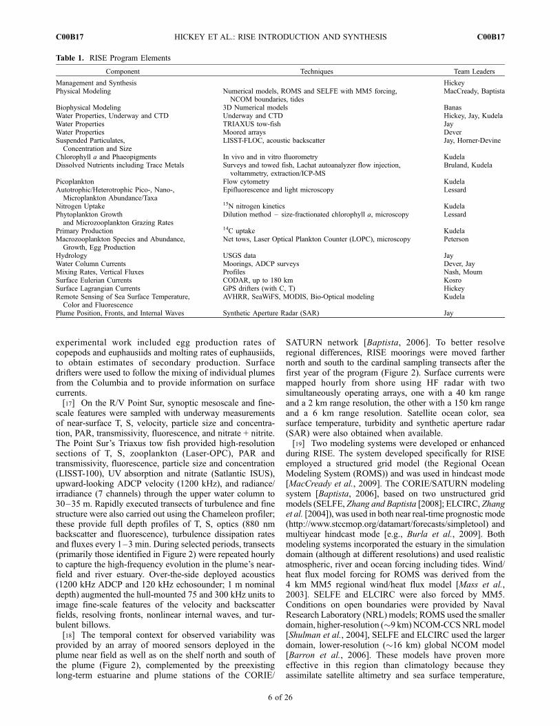
in the Pacific Northwest during the RISE summers [Shaw etal., 2009], consistent with the occurrence of positive phasesof MEI and PDO. The fact that the warmer water is relatedto advection rather than local heating is confirmed with timeseries of copepod species assemblages (Figure 5). In anaverage year, during winter months the northward flowingDavidson Current transports warm water ‘‘neritic’’ species(species restricted to coastal shelf environments) northwardfrom California to the Oregon and Washington shelves;during the upwelling season, cold water species usuallydominate and these species are transported southward fromcoastal British Columbia and the coastal Gulf of Alaska.During the RISE project summers of 2003 through 2005 thecopepod communitywas dominated by ‘‘warmwater neritic’’species, as typically occurs when the PDO is positive [Hooffand Peterson, 2006]. The community began to transition to

a cold water species phase during the summer of 2006,consistent with the decreasing PDO (Figure 3); however‘‘warm water oceanic’’ species were still conspicuous insamples. Figure 3 also shows that during strong El Ninoevents (as in late 1997–1998) the copepod community isalso dominated entirely by warm water species (for bothneritic and oceanic species). Thus, the RISE years weresimilar in some respects [biological (zooplankton) andphysical (riverflow and surface water temperatures)] to ElNino conditions.[24] In spite of the low overall riverflow and El Nino-like

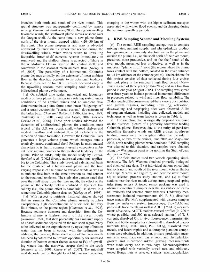
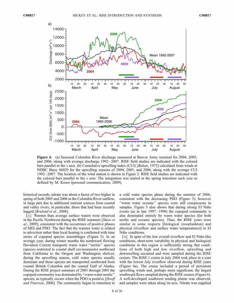
conditions, short-term variability in physical and biologicalconditions in this region is sufficiently strong that condi-tions of both high and low riverflow, upwelling anddownwelling occurred and were sampled during the RISEcruises. The RISE 1 cruise in July 2004 took place in a yearwith the lowest July riverflow observed during RISE years(Figure 4a). The cruise included a period of persistentupwelling winds and, perhaps more significant, the largestsouthward flows sampled during the RISE cruises (Figure 6).A well-developed southwest tending plume was observed,and samples were taken along its axis. Nitrate was supplied

Figure 4. (a) Seasonal Columbia River discharge measured at Beaver Army terminal for 2004, 2005,and 2006, along with average discharge 1992–2007. RISE field studies are indicated with the coloredbars parallel to the x axis. (b) Cumulative upwelling index (CUI) [Bakun, 1973] calculated from winds atNDBC Buoy 46029 for the upwelling seasons of 2004, 2005, and 2006, along with the average CUI1992–2007. The location of the wind station is shown in Figure 2. RISE field studies are indicated withthe colored bars parallel to the x axis. The integration was started at the spring transition each year asdefined by M. Kosro (personal communication, 2009).


8 of 26

C00B17

to the plume via upwelled nitrate-rich waters mixingwith nitrate-depleted river water during plume formation[Bruland et al., 2008]. Seasonal upwelling favorable windsprior to the cruise were the weakest observed during RISEyears (Figure 4b).[25] In 2005, upwelling over the inner shelf was delayed

[Hickey et al., 2006; Kosro et al., 2006] and the May–June

RISE 2 cruise took place prior to the onset of strongupwelling favorable winds and just after a period of higherthan average riverflow (Figures 4a and 6). Aweak southwesttending plume was observed at the beginning of the cruise,but most cruise sampling took place in a northward tendingplume. Plume nutrients were being supplied from the water-shed rather than from the coastal ocean [Bruland et al., 2008],

Figure 5. Proportion of copepod community types in zooplankton tows at a station 9 km offshore onthe Newport line (44�39.10N, 124�10.60W). The length of each color bar is proportional to the amount ofthat taxa. Data acquired from Peterson Lab.

Figure 6. Alongshelf component (positive northward) of wind at Buoy 46029 and near-surface currentat mooring RN, north of the Columbia mouth (see location in Figure 2) for each of the RISE fieldseasons. The shipboard field studies are shown with shaded bars. Sections from the ‘‘cardinal’’ samplingtransects offshore of Grays Harbor (G) and Cape Meares (C) are indicated with vertical lines. Satellitedata used in this paper (Figure 1) are indicated (S) along with times of model runs displayed in Figure 10(M). Current data provided by Dever Lab.


9 of 26

C00B17

resulting in substantially lower than expected coastal pro-ductivity [Kudela et al., 2006].[26] RISE 3 took place in August 2005 in a period with

the lowest riverflow of all the RISE cruises (Figure 4a) andafter upwelling favorable winds had become persistent(Figures 4b and 6). A strong well-developed southwestplume was observed and sampled. This was the onlyobservation of actual upwelling off the Washington coastin all of the RISE cruises. Plume nutrients were beingprovided from upwelling water that mixed with the out-flowing riverflow [Bruland et al., 2008].[27] The final RISE cruise took place in May–early June

2006 under extremely high riverflow conditions, the highestobserved in the four RISE cruises (Figure 4a). Downwellingfavorable winds were also higher than typically observed atthat time of year as indicated by the significant dip in thecumulative wind stress curve during the cruise period(Figures 4b and 6). The majority of the cruise time wasused sampling north tending plumes, following the plumesas far north as the Strait of Juan de Fuca [Hickey et al.,2009]. However, a new southwest tending plume developedduring the last few days of the cruise. In that period, theriver itself was supplying plume nutrients to both north andsouthwest tending plumes [Bruland et al., 2008]. Surfacedrifters were used to follow the newly emerging southwestplume, sampling its chemical and biological aging withcross-plume transects [Hickey et al., 2009].

5. RISE Results

[28] Several key issues on the development, evolutionand importance of river plumes to the regional ecosystemremained at the outset of RISE. One of the least understoodphenomena with respect to river plumes was how thefreshwater discharge mixes with ambient coastal waters[Boicourt et al., 1998; Wiseman and Garvine, 1995].Another important issue was the effect of a buoyant plumeon local transport pathways. A third critical issue wascaptured by the overall RISE question: how does a buoyantplume impact the ecosystem? The results of RISE as theypertain to these important issues, as well as our ability tomodel these processes and impacts are summarized below.

5.1. Regional Plume Effects

5.1.1. Does the Plume Alter Phytoplankton GrowthRates, Grazing Rates, or Species Compositionin Comparison to Active Upwelling Regions?

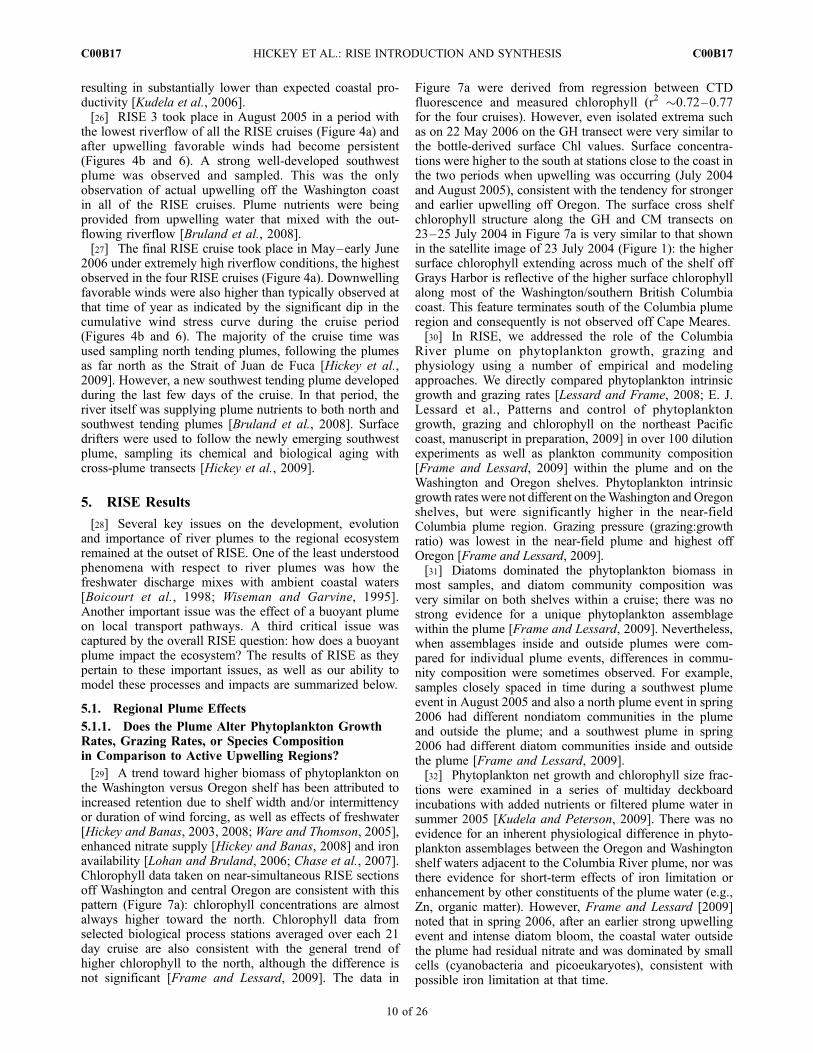
[29] A trend toward higher biomass of phytoplankton onthe Washington versus Oregon shelf has been attributed toincreased retention due to shelf width and/or intermittencyor duration of wind forcing, as well as effects of freshwater[Hickey and Banas, 2003, 2008; Ware and Thomson, 2005],enhanced nitrate supply [Hickey and Banas, 2008] and ironavailability [Lohan and Bruland, 2006; Chase et al., 2007].Chlorophyll data taken on near-simultaneous RISE sectionsoff Washington and central Oregon are consistent with thispattern (Figure 7a): chlorophyll concentrations are almostalways higher toward the north. Chlorophyll data fromselected biological process stations averaged over each 21day cruise are also consistent with the general trend ofhigher chlorophyll to the north, although the difference isnot significant [Frame and Lessard, 2009]. The data in

Figure 7a were derived from regression between CTDfluorescence and measured chlorophyll (r2 �0.72–0.77for the four cruises). However, even isolated extrema suchas on 22 May 2006 on the GH transect were very similar tothe bottle-derived surface Chl values. Surface concentra-tions were higher to the south at stations close to the coast inthe two periods when upwelling was occurring (July 2004and August 2005), consistent with the tendency for strongerand earlier upwelling off Oregon. The surface cross shelfchlorophyll structure along the GH and CM transects on23–25 July 2004 in Figure 7a is very similar to that shownin the satellite image of 23 July 2004 (Figure 1): the highersurface chlorophyll extending across much of the shelf offGrays Harbor is reflective of the higher surface chlorophyllalong most of the Washington/southern British Columbiacoast. This feature terminates south of the Columbia plumeregion and consequently is not observed off Cape Meares.[30] In RISE, we addressed the role of the Columbia

River plume on phytoplankton growth, grazing andphysiology using a number of empirical and modelingapproaches. We directly compared phytoplankton intrinsicgrowth and grazing rates [Lessard and Frame, 2008; E. J.Lessard et al., Patterns and control of phytoplanktongrowth, grazing and chlorophyll on the northeast Pacificcoast, manuscript in preparation, 2009] in over 100 dilutionexperiments as well as plankton community composition[Frame and Lessard, 2009] within the plume and on theWashington and Oregon shelves. Phytoplankton intrinsicgrowth rates were not different on theWashington and Oregonshelves, but were significantly higher in the near-fieldColumbia plume region. Grazing pressure (grazing:growthratio) was lowest in the near-field plume and highest offOregon [Frame and Lessard, 2009].[31] Diatoms dominated the phytoplankton biomass in

most samples, and diatom community composition wasvery similar on both shelves within a cruise; there was nostrong evidence for a unique phytoplankton assemblagewithin the plume [Frame and Lessard, 2009]. Nevertheless,when assemblages inside and outside plumes were com-pared for individual plume events, differences in commu-nity composition were sometimes observed. For example,samples closely spaced in time during a southwest plumeevent in August 2005 and also a north plume event in spring2006 had different nondiatom communities in the plumeand outside the plume; and a southwest plume in spring2006 had different diatom communities inside and outsidethe plume [Frame and Lessard, 2009].[32] Phytoplankton net growth and chlorophyll size frac-

tions were examined in a series of multiday deckboardincubations with added nutrients or filtered plume water insummer 2005 [Kudela and Peterson, 2009]. There was noevidence for an inherent physiological difference in phyto-plankton assemblages between the Oregon and Washingtonshelf waters adjacent to the Columbia River plume, nor wasthere evidence for short-term effects of iron limitation orenhancement by other constituents of the plume water (e.g.,Zn, organic matter). However, Frame and Lessard [2009]noted that in spring 2006, after an earlier strong upwellingevent and intense diatom bloom, the coastal water outsidethe plume had residual nitrate and was dominated by smallcells (cyanobacteria and picoeukaryotes), consistent withpossible iron limitation at that time.


10 of 26

C00B17

[33] The alongshore difference in grazing pressure(higher off Oregon than off Washington) likely plays asignificant role in maintaining higher chlorophyll concen-trations on the Washington shelf [Lessard and Frame, 2008;Lessard et al., manuscript in preparation, 2009]. In addition,model results show that the plume forms a ‘‘barrier’’ tobiomass transport to Oregon, deflecting up to 20% of thephytoplankton biomass offshore (see below) [Banas et al.,2009b]. The wider shelf north of the Columbia (affectingretention patterns and possible bloom spin-up times) as wellas the retentive characteristics of the Juan de Fuca eddy that

feeds the Washington shelf from the north also play impor-tant roles in producing alongcoast spatial gradients inchlorophyll [Hickey and Banas, 2008].[34] Historical data suggest that the abundance of macro-

zooplankton such as copepods and euphausiids is higher offthe Washington coast (north of the Columbia Riverentrance) than south of it (net tow data, Landry andLorenzen [1989]; acoustic data, Swartzman and Hickey[2003]). Swartzman [2001] shows higher abundances overWashington canyons, leading to the commonly expoundedidea that the higher abundances are related to the greater

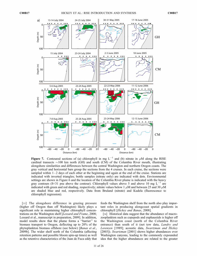
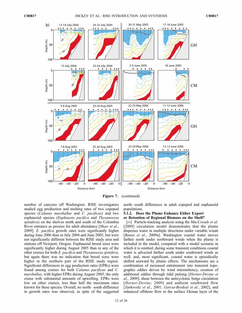
Figure 7. Contoured sections of (a) chlorophyll in mg L�1 and (b) nitrate in mM along the RISEcardinal transects �100 km north (GH) and south (CM) of the Columbia River mouth, illustratingalongshore similarities and differences between the central Washington and northern Oregon coasts. Thegray vertical and horizontal bars group the sections from the 4 cruises. In each cruise, the sections weresampled within 1–2 days of each other at the beginning and again at the end of the cruise. Stations areindicated with inverted triangles; bottle samples (nitrate only) are indicated with dots. Environmentalsettings are shown in Figure 6 and the location of the Columbia River plume is indicated with the heavygray contours (S<31 psu above the contour). Chlorophyll values above 5 and above 10 mg L�1 areindicated with green and red shading, respectively; nitrate values below 1 mM and between 25 and 30 mMare shaded blue and red, respectively. Data from Bruland (nitrate) and Kudela (fluorescence tochlorophyll regression).


11 of 26

C00B17

number of canyons off Washington. RISE investigatorsstudied egg production and molting rates of two copepodspecies (Calanus marshallae and C. pacificus) and twoeuphausiid species (Euphausia pacifica and Thysanoessaspinifera) on the shelves north and south of the ColumbiaRiver entrance as proxies for adult abundance [Shaw et al.,2009]. E. pacifica growth rates were significantly higherduring June 2006 than in July 2004 and June 2005, but werenot significantly different between the RISE study area andstations off Newport, Oregon. Euphausiid brood sizes weresignificantly higher during August 2005 than in any of theother cruises for both E. pacifica and Thysanoessa spinifera,but again there was no indication that brood sizes werehigher in the northern part of the RISE study region.Significant differences in egg production rates (EPRs) werefound among cruises for both Calanus pacificus and C.marshallae, with higher EPRs during August 2005, the onlycruise with substantial amounts of upwelling. EPRs werelow on other cruises, less than half the maximum ratesknown for these species. Overall, no north–south differencein growth rates was observed, in spite of the suggested

north–south differences in adult copepod and euphausiidpopulations.5.1.2. Does the Plume Enhance Either Exportor Retention of Regional Biomass on the Shelf?[35] Particle-tracking analysis using the MacCready et al.

[2009] circulation model demonstrates that the plumedisperses water in multiple directions under variable winds[Banas et al., 2009a]. Washington coastal water movesfarther north under northward winds when the plume isincluded in the model, compared with a model scenario inwhich it is omitted; during some transient conditions coastalwater is advected farther south under southward winds aswell; and, most significant, coastal water is episodicallyshifted seaward by plume effects. The mechanisms are acombination of increased entrainment into transient topo-graphic eddies driven by wind intermittency, creation ofadditional eddies through tidal pulsing [Horner-Devine etal., 2009], shear between the anticyclonic bulge circulation[Horner-Devine, 2009] and ambient southward flow[Yankovsky et al., 2001; Garcia-Berdeal et al., 2002], andenhanced offshore flow in the surface Ekman layer of the

Figure 7. (continued)


12 of 26

C00B17

plume, which is vertically compressed by the plumestratification [Garcia-Berdeal et al., 2002]. The net effectof these processes during a model hindcast of July 2004 wasto export 25% more water from the Washington inner shelfpast the 100 m isobath, when the plume was included in themodel versus when it was not [Banas et al., 2009a].[36] This net export of water is reflected in a seaward

shift in biomass and primary production in the Banas et al.[2009b] biophysical model as well. Inclusion of the plumewas found to decrease primary production on the inner shelfby 20% under weak to moderate upwelling favorable winds,and simultaneously to increase primary production on theouter shelf and slope by 10–20%. This seaward shift mainlyreflects a shift in biomass distribution, rather than a shift ingrowth rates or spatially integrated production.[37] Empirical data of macrozooplankton-sized particle

distribution and chlorophyll fluorescence from the May2005 survey [Peterson and Peterson, 2008, Figure 1] areconsistent with the model results: maximum zooplanktonabundance and chlorophyll fluorescence follow the path ofthe southward tending plume. North of the plume, maxi-mum values occur between the 50 and 100 m isobath. Southof the river mouth, the maxima are shifted offshore, extend-ing to the outer shelf and slope. With the available data,however, localized growth and aggregation cannot be dis-tinguished from advective processes. In proximity to theriver mouth, aggregations of zooplankton can be pushedacross the shelf at velocities up to 38 cm s–1, roughlyfivefold faster than typical wind-driven Ekman transport inthe region [Peterson and Peterson, 2009].[38] Under some conditions, the plume can also enhance

retention of water and biomass [Hickey and Banas, 2008].For example, on the inner shelf north of the river mouthretention typically occurs after a well-developed northtending plume that was formed during a period ofdownwelling favorable winds moves away from the coastduring a subsequent period of upwelling favorable winds:the shoreward plume front forms a barrier to cross-shelftransport. Model studies also suggest [Banas et al., 2009a,2009b] that interactions between the plume and variablewinds episodically retard the equatorward advection ofbiomass from the Washington shelf, so that the plume actsas a retention feature in an alongcoast sense as well [Hickeyand Banas, 2008].5.1.3. Does the Plume Spatially Concentrate Plankton?If So, Where?[39] Broad-scale and fine-scale surveys with a Triaxus

tow body equipped with a Laser Optical Plankton Counterand CTD provided a detailed picture of the relationshipbetween plume waters and macrozooplankton-sized particledistributions. Overall, vertically integrated zooplankton-sized particle abundance and biovolume were elevated inproximity to ‘‘aged’’ plume waters (i.e., surface salinitybetween 25 and 30). Integrated abundance was approxi-mately 7 � 106 particles m�2 in proximity to ‘‘aged’’ plumewaters, and 4 � 106 particles m�2 outside these areas. Inaddition, zooplankton tended to aggregate near the surface(upper 10 m) in proximity to river plume waters and weredeeper in the water column (25 m) when the plume was notpresent [Peterson and Peterson, 2009].[40] Analysis of the evolution of salinity following

drifters released at the estuary mouth during maximum

ebb shows that plume surface water overtakes the plumefront [McCabe et al., 2008, 2009], clearly indicating that thefront is a surface convergence feature. Fine-scale surveysacross the plume front revealed that during a strong ebbtide, zooplankton-sized particles were up to twofold moreconcentrated on the seaward side of the plume frontcompared to concentrations 3 km on either side of the front[Peterson and Peterson, 2009]. Physical processes associ-ated with the developing plume vertically depressed denselayers of phytoplankton and zooplankton an average of 7 mdeeper into the water column both beneath the plume and upto 10 km seaward of the plume front; this feature may beassociated with plume-related nonlinear internal waves (seesection 5.3.3).5.1.4. Do Nutrients Supplied by the Plume EnhanceProductivity on a Regional Basis?[41] Nitrate and other nutrients are upwelled onto the

shelf seasonally. Upwelling favorable wind stress decreasesnorthward by about a factor of two over the RISE region.RISE nitrate data illustrate that in spite of this decline,nitrate concentrations below the surface layer (�20 m)across the shelf are as high or higher toward the north inthe RISE region (Figure 7b). In the upper water column,alongcoast nitrate can be higher to the north or to the south,a result of biological drawdown (Figure 7b).[42] During periods of strong upwelling favorable winds

when the Columbia River plume is directed southwest offthe Oregon shelf, upwelled nitrate from the shelf mixed intothe plume in the estuary and near the river mouth is thedominant source of nutrients in the plume. During periodsof downwelling, when isopycnals and associated highvalues of nitrate move downward and offshore, this supplyroute is eliminated. Unlike the Mississippi River, nitratesupply to the plume from its watershed is low in summer[Conomos et al., 1972; Sullivan et al., 2001]. However, insome spring periods, particularly when rainfall is higherthan normal, elevated nitrate concentrations from thewatershed can be delivered to the ocean by the high river-flow [Bruland et al., 2008]. A seasonal nitrate budget forthis region suggests that nitrate input from the Columbiawatersheds is two orders of magnitude smaller than inputfrom coastal upwelling, from the Strait of Juan de Fuca orfrom submarine canyons [Hickey and Banas, 2008].Although small in comparison to other sources on asummer-averaged basis, watershed-derived nutrients mayhelp sustain the ecosystem during periods of delayedseasonal upwelling, as occurred in 2005 [Hickey and Banas,2008] and also during periods of downwelling. Thus,whereas nitrate supply on the Oregon coast is shut offduring downwelling or weak winds, the Washington coasthas an additional supply from the Columbia River to helpmaintain productivity during such periods.[43] Recent measurements indicate that whereas iron can

be a limiting nutrient off California [Hutchins and Bruland,1998; Hutchins et al., 1998; Bruland et al., 2001; Firme etal., 2003], phytoplankton growth has not been observed tobe iron limited off the Oregon coast [Chase et al., 2002].RISE studies have shown that iron is not generally limitingon the Washington coast [Kudela and Peterson, 2009;Lohan and Bruland, 2006, 2008; Bruland et al., 2008].Not only is the plume from the Columbia heavily laden withiron, particulate iron from the Columbia plume is also


13 of 26

C00B17

deposited in midshelf sediments along both the Washingtonand Oregon coasts. The iron-laden shelf sediment can bemixed into bottom water and thus added to the alreadynitrate-rich water during coastal upwelling [Lohan andBruland, 2008].[44] A biological model study comparing results with and

without a river plume has shown that more nitrate isprovided to the sea surface, and more biomass accumulatesin the region near the river mouth when the river plume ispresent [Hickey and Banas, 2008]. The enhancement is duenot to the river itself, but to enhanced mixing by the large

tidal currents near the river mouth. Similar effects were seenjust offshore of Washington’s other two coastal estuaries.5.1.5. Does Phytoplankton Size Differ Between ShelvesNorth and South of the River Mouth?[45] On three of four RISE cruises size fractionated

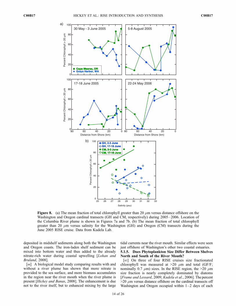
chlorophyll was measured at >20 mm and total (GF/F;nominally 0.7 mm) sizes. In the RISE region, the >20 mmsize fraction is nearly completely dominated by diatoms[Frame and Lessard, 2009; Kudela et al., 2006]. The percent>20 mm versus distance offshore on the cardinal transects offWashington and Oregon occupied within 1–2 days of each

Figure 8. (a) The mean fraction of total chlorophyll greater than 20 mm versus distance offshore on theWashington and Oregon cardinal transects (GH and CM, respectively) during 2005–2006. Location ofthe Columbia River plume is shown in Figures 7a and 7b. (b) The mean fraction of total chlorophyllgreater than 20 mm versus salinity for the Washington (GH) and Oregon (CM) transects during theJune 2005 RISE cruise. Data from Kudela Lab.


14 of 26

C00B17

other is shown in Figure 8a. The presence or absence of aColumbia plume on these transects is indicated with a graycontour on chlorophyll and nitrate sections in Figures 7aand 7b. The left-hand panels in Figure 8a illustrate cross-shelf structure during periods when the Columbia plumewas observed on both transects; the right-hand panelsillustrate structure during periods of upwelling, although aplume is present off Oregon (CM transect) during May–June 2006.[46] Comparison between transects sampled at the start

and end of the cruise in May–June 2005 (Figure 8a, left)indicates significant temporal variability over periods of10–15 days. On that cruise, the percent of large cells within�30 km of the Oregon coast (CM transect) decreasedsignificantly from 60 to 90% to 25–40% over the 2–3 weekperiod between repeat transect sampling.[47] Significant spatial differences were observed

between Washington and Oregon within 20–30 km of thecoast during periods when the Columbia plume was present.In particular, the percent of large cells was smaller off theWashington coast (GH) at most stations (Figure 8a, left). Incontrast, during periods when upwelling had recentlyoccurred or was active, the percent of large cells was similaroff the two coasts (Figure 8a, right). A two-tail Student’s ttest (assuming unequal variances) applied on all data closerthan 25 km from shore, for all four cruises and bothWashington (GH) and Oregon (CM) transects (n = 16 andn = 17 for >20 and >5 mm, respectively) gave p = 0.001 andp = 0.018 for the 20 and 5 mm size ranges, respectively, withthe percent of large cells higher off Oregon. This is a veryconservative test, indicating that the results are highlysignificant.[48] Figure 8a also shows that although cell size frequently

decreases from nearshore to offshore [Kudela et al., 2006],this pattern was altered in the presence of a plume: cell sizeappears to increase with distance offshore on the GHtransect (upper left panel). This phenomenon is depictedexplicitly in Figure 8b, where percent >20 mm is plottedagainst salinity for the May–June 2005 cruise, duringwhich the plume was observed on all transects. The percentof large cells increases significantly with salinity followingthe plume as it becomes saltier (i.e., ‘‘aging’’) on the firstoccupations of both Washington (GH) and Oregon (CM)transects (r = 0.74, 0.75, for CM and GH, respectively,significant at the 95% level), with higher percentages oflarge cells off Oregon. On the second occupations of thesetransects, high salinity water (S>31 psu) appeared on theoffshore ends of sections (likely originating in the Strait ofJuan de Fuca; MacFadyen et al. [2008]); the slope of theGH transect data is not significant, and the slope of the CMtransect is significant, but negative. Thesewaters were clearlydominated by smaller cells, and the dilution with this newwater masked any increase in cell size with aging Columbiaplume water in the regression. Based on these data, it appearsthat size structure is more affected by physical processes(upwelling and plume formation) than by latitude.5.1.6. Does Turbidity Influence PhytoplanktonPhotosynthesis?[49] In contrast to expectations, there was not a strong

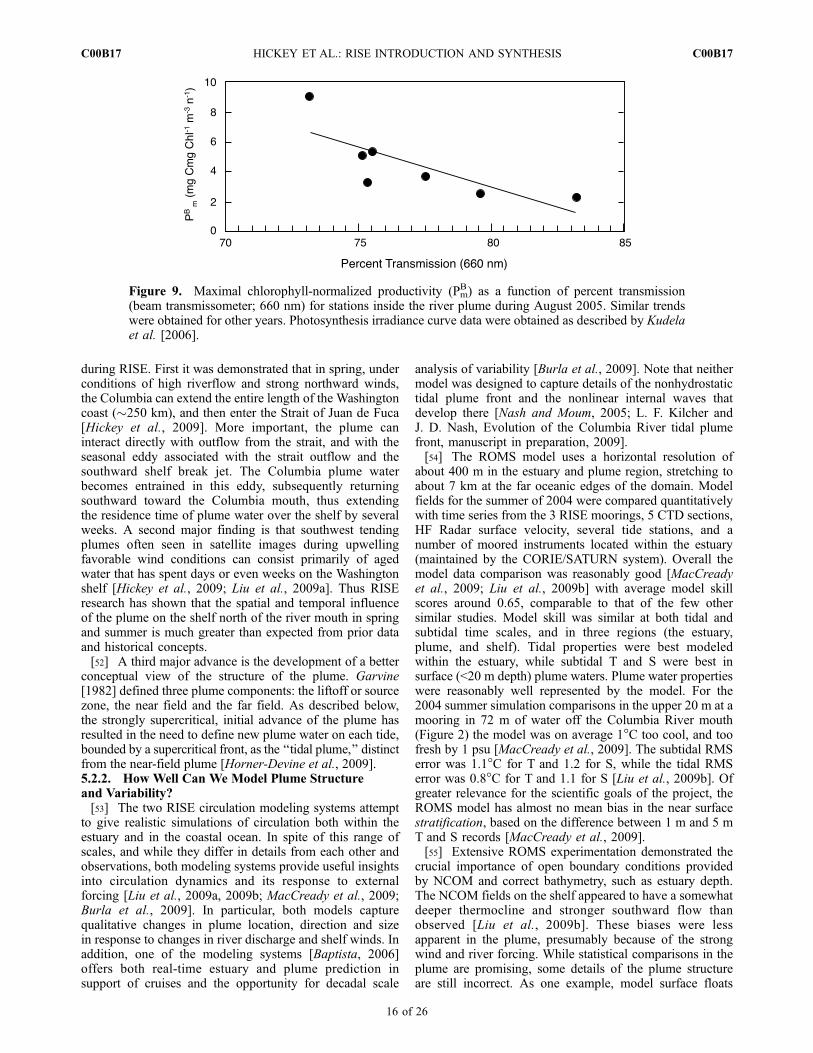
response in phytoplankton photosynthesis versus irradiance(PE) kinetics from stations within the plume. PE curvescollected near surface (2 m) and near bottom in the near-

field plume were generally indistinguishable from eachother (p>0.05), with more variability between consecutiveebb pulses (temporal variability) than with depth (R. M.Kudela, unpublished data, 2009). In fact, within each cruise,there was a significantly positive relationship betweenincreasing turbidity and increasing maximal chlorophyll-normalized productivity (r = 0.78, significant at the 95%level) (Figure 9). There was also a negative correlation oflight transmission with both iron and nitrate concentrations,suggesting that the effects of turbidity on carbon assimila-tion were either not significant, or were overcome by theco-occurring increase in nutrients. During August 2005ambient nitrate was in excess of the measured half-satu-ration parameter for nitrate uptake (Ks) for 5 of 7 PEcurves [Kudela and Peterson, 2009], while the remainingtwo stations exhibited elevated carbon assimilation andturbidity (i.e., opposite expectations if the trend is a functionof nitrate concentration), suggesting that plume turbiditydoes not have a negative impact on photosynthesis. Multi-day deckboard incubations during August 2005 also showedno evidence for iron limitation either within or outside theplume [Kudela and Peterson, 2009]. Similar results havebeen reported for plumes in Lake Michigan, where Lohrenzet al. [2004] reported no effect on phytoplankton productioninside and outside a persistent turbidity plume. Both theLake Michigan and Columbia River plumes are dominatedby particle scattering rather than absorption (e.g., due tocolored dissolved material); this appears to result in a highturbidity, diffuse light environment that has relatively littleimpact on photosynthesizing organisms.5.1.7. What is the Origin of Plume Turbidity in Springand Summer?[50] Detailed measurements of sediment fluxes into and

out of the plume in the near-field region highlight animportant seasonal trend in the origin of sediment enteringthe plume [Spahn et al., 2009]. During the spring freshet ofMay 2006, delivery of sediment to the plume from the riverwas relatively high and strong vertical stratification pre-vented sediment from the seabed in the near-field regionfrom entering the plume directly. In contrast, data from theend of the summer in August 2005 show a decrease of inputfrom the river. Under these low flow conditions the near-field plume is much less stratified and strongly interactswith the bottom, generating bottom-attached fronts charac-terized by elevated turbulence and vertical velocity, whichcarry resuspended sediment from the seabed toward thesurface plume waters. Thus, the data suggest that sedimentsentering the plume originate primarily from the river inspring and increasingly from the seabed through thesummer. This result is consistent with dissolved and labileparticulate iron measurements in August 2005 and May2006, which also show a shift from fluvial to marine sourcesover the course of the summer [Bruland et al., 2008; S. M.Lippiatt et al., Leachable particulate iron in the ColumbiaRiver, estuary and near-field plume, submitted to EstuarineCoastal Shelf Science, 2009].

5.2. Regional Plume Structure and Modeling

5.2.1. What is the Spatial and Temporal Extentof the Plume in Spring/Summer?

[51] Three major advancements in our understanding ofColumbia plume extent, location and structure were made


15 of 26

C00B17

during RISE. First it was demonstrated that in spring, underconditions of high riverflow and strong northward winds,the Columbia can extend the entire length of the Washingtoncoast (�250 km), and then enter the Strait of Juan de Fuca[Hickey et al., 2009]. More important, the plume caninteract directly with outflow from the strait, and with theseasonal eddy associated with the strait outflow and thesouthward shelf break jet. The Columbia plume waterbecomes entrained in this eddy, subsequently returningsouthward toward the Columbia mouth, thus extendingthe residence time of plume water over the shelf by severalweeks. A second major finding is that southwest tendingplumes often seen in satellite images during upwellingfavorable wind conditions can consist primarily of agedwater that has spent days or even weeks on the Washingtonshelf [Hickey et al., 2009; Liu et al., 2009a]. Thus RISEresearch has shown that the spatial and temporal influenceof the plume on the shelf north of the river mouth in springand summer is much greater than expected from prior dataand historical concepts.[52] A third major advance is the development of a better

conceptual view of the structure of the plume. Garvine[1982] defined three plume components: the liftoff or sourcezone, the near field and the far field. As described below,the strongly supercritical, initial advance of the plume hasresulted in the need to define new plume water on each tide,bounded by a supercritical front, as the ‘‘tidal plume,’’ distinctfrom the near-field plume [Horner-Devine et al., 2009].5.2.2. How Well Can We Model Plume Structureand Variability?[53] The two RISE circulation modeling systems attempt

to give realistic simulations of circulation both within theestuary and in the coastal ocean. In spite of this range ofscales, and while they differ in details from each other andobservations, both modeling systems provide useful insightsinto circulation dynamics and its response to externalforcing [Liu et al., 2009a, 2009b; MacCready et al., 2009;Burla et al., 2009]. In particular, both models capturequalitative changes in plume location, direction and sizein response to changes in river discharge and shelf winds. Inaddition, one of the modeling systems [Baptista, 2006]offers both real-time estuary and plume prediction insupport of cruises and the opportunity for decadal scale

analysis of variability [Burla et al., 2009]. Note that neithermodel was designed to capture details of the nonhydrostatictidal plume front and the nonlinear internal waves thatdevelop there [Nash and Moum, 2005; L. F. Kilcher andJ. D. Nash, Evolution of the Columbia River tidal plumefront, manuscript in preparation, 2009].[54] The ROMS model uses a horizontal resolution of

about 400 m in the estuary and plume region, stretching toabout 7 km at the far oceanic edges of the domain. Modelfields for the summer of 2004 were compared quantitativelywith time series from the 3 RISE moorings, 5 CTD sections,HF Radar surface velocity, several tide stations, and anumber of moored instruments located within the estuary(maintained by the CORIE/SATURN system). Overall themodel data comparison was reasonably good [MacCreadyet al., 2009; Liu et al., 2009b] with average model skillscores around 0.65, comparable to that of the few othersimilar studies. Model skill was similar at both tidal andsubtidal time scales, and in three regions (the estuary,plume, and shelf). Tidal properties were best modeledwithin the estuary, while subtidal T and S were best insurface (<20 m depth) plume waters. Plume water propertieswere reasonably well represented by the model. For the2004 summer simulation comparisons in the upper 20 m at amooring in 72 m of water off the Columbia River mouth(Figure 2) the model was on average 1�C too cool, and toofresh by 1 psu [MacCready et al., 2009]. The subtidal RMSerror was 1.1�C for T and 1.2 for S, while the tidal RMSerror was 0.8�C for T and 1.1 for S [Liu et al., 2009b]. Ofgreater relevance for the scientific goals of the project, theROMS model has almost no mean bias in the near surfacestratification, based on the difference between 1 m and 5 mT and S records [MacCready et al., 2009].[55] Extensive ROMS experimentation demonstrated the

crucial importance of open boundary conditions providedby NCOM and correct bathymetry, such as estuary depth.The NCOM fields on the shelf appeared to have a somewhatdeeper thermocline and stronger southward flow thanobserved [Liu et al., 2009b]. These biases were lessapparent in the plume, presumably because of the strongwind and river forcing. While statistical comparisons in theplume are promising, some details of the plume structureare still incorrect. As one example, model surface floats

Figure 9. Maximal chlorophyll-normalized productivity (PmB) as a function of percent transmission

(beam transmissometer; 660 nm) for stations inside the river plume during August 2005. Similar trendswere obtained for other years. Photosynthesis irradiance curve data were obtained as described by Kudelaet al. [2006].


16 of 26

C00B17

released near the Columbia River mouth on ebb tide did notpenetrate as far seaward as field drifters deployed duringRISE observational campaigns [McCabe et al., 2008].Select numerical experiments also illustrated that float-tracked surface plume water may become too salty (meansalinity excess of �3–4 psu). Other investigators havefound similar results in recent estuarine applications [e.g.,Warner et al., 2005; Li et al., 2005]. The tidal plume ischaracterized by extremely high shear and stratification andremains one of the most difficult to model physical environ-ments in the coastal zone. A hydrostatic model like ROMSnecessarily omits details of the plume front and the non-linear internal waves it generates. Because of this we cannotsimulate a potentially large source of observed plumemixing.[56] The CORIE/SATURN modeling system is built with

the philosophy of redundancy in model, grids/domains, andmodeling parameterizations. For any given period, dailyforecasts and multiyear simulation databases are conductedfor at least two domains (river-to-ocean and either estuary-only or estuary/near plume), with river-to-ocean simulationsconducted with two models: SELFE [Zhang and Baptista,2008] and ELCIRC [Zhang et al., 2004]; only SELFE isused for the estuary-only and estuary/near plume domains.Simulations often explore multiple parameterizations andthe option exists to use model-independent data assimilationstrategies [Frolov et al., 2009a] for either improved processunderstanding [Frolov et al., 2009b] or observational net-work optimization [Frolov et al., 2008]. Skill assessmenthas been conducted for simulations based on both ELCIRC[Baptista et al., 2005; Burla et al., 2009] and SELFE[Zhang and Baptista, 2008; Burla et al., 2009], and quan-titative skill assessment metrics have recently become a partof routine processing of all forecasts and simulation data-bases in the CORIE/SATURN modeling system (http://www.stccmop.org). Quantitative skill metrics are based oncomparisons with both routine CORIE/SATURN observa-tions and observations of opportunity (such as RISEmoorings and cruises). Highest skill is typically achievedwith SELFE rather than with ELCIRC, and (although oftenmarginally) with hindcasts versus forecasts; during a typicalcruise, forecast skill was high enough to direct vesselswithin 2 km of a predicted concentration more than 55%of the time (Zhang and Baptista, personal communication,2009).[57] Typical SELFE/ELCIRC grid resolution is �150 m

in the estuary, 250 m–1 km in the near plume, and 3 km–20 km in the far plume. Skill typically decreases from theestuary to the plume to the shelf outside the near-fieldplume, reflecting at least in part the different resolution ineach of these regions. For the plume, ELCIRC simulationshave shown a tendency for excess freshness (e.g., as arelatively extreme example, for 2004 the ELCIRC modelbias for salinity at a shelf mooring near the river mouth was�2.9 psu, versus just �0.2 for SELFE) [see Burla et al.,2009]. SELFE was thus the preferred CORIE/SATURNmodel for both near real-time forecasts in support ofoceanographic cruises and the calculation of multiyear timeseries plume characteristics such as volume, area, thicknessand centroid location [Burla et al., 2009].[58] Although a systematic comparison between

the ROMS and SELFE model implementations for the

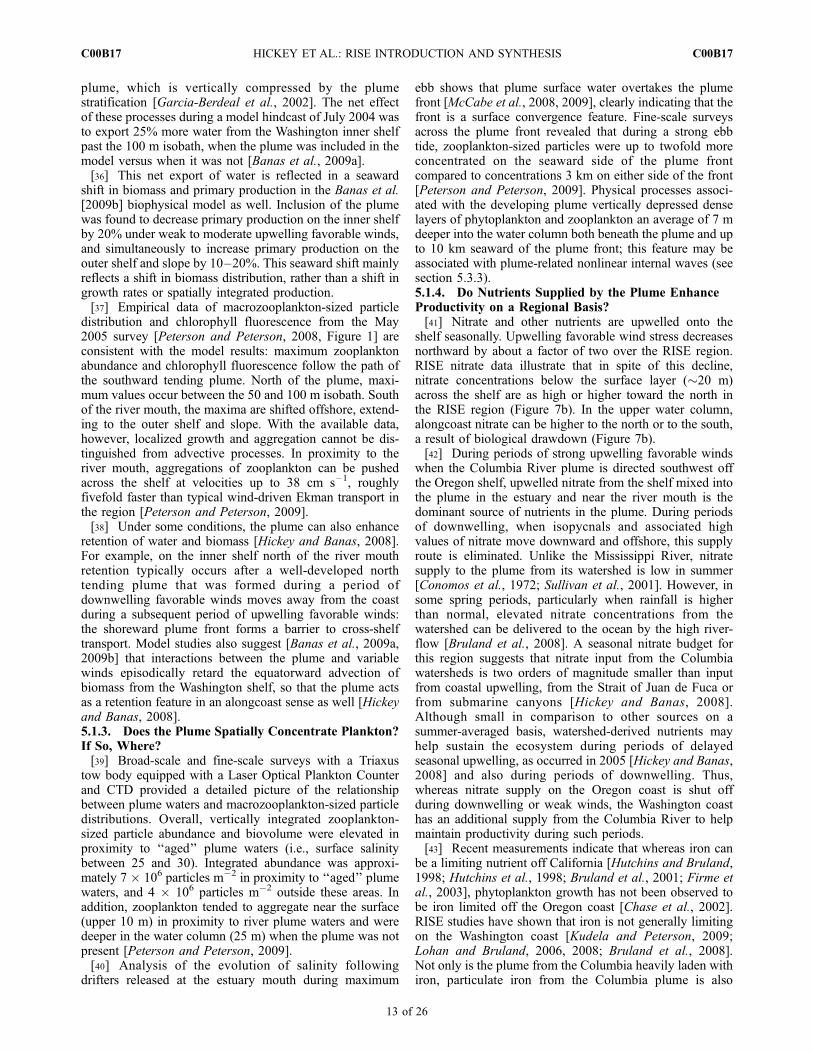
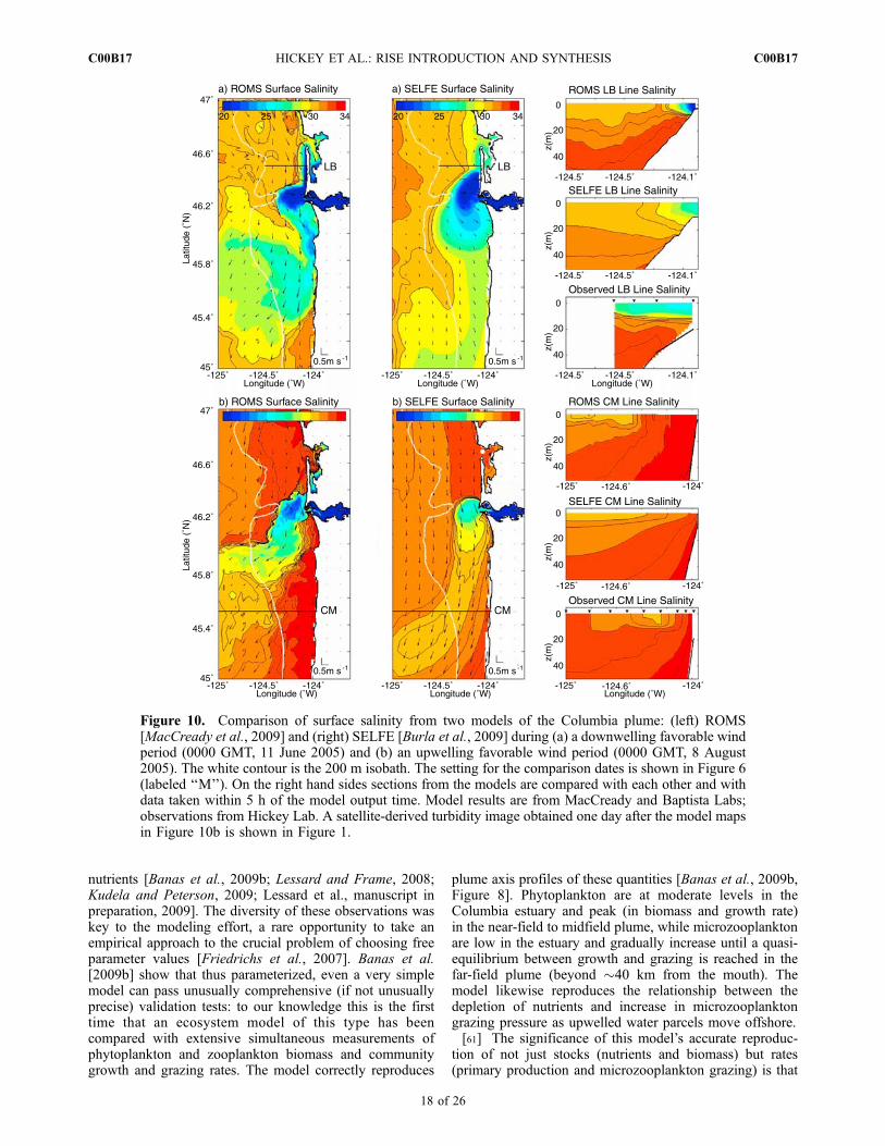
Columbia plume has not been performed to date, examplesof their salinity and velocity fields are compared inFigure 10 for (1) a period when the plume tends northwardand (2) a period when the plume tends to the southwest. Themodel runs were selected for dates when CTD transects areavailable. In addition, satellite imagery (Figure 1) is avail-able within one day of the second model runs. Model mapsrepresent snapshots while CTD data are taken over severalhours. For the LB section, total time is 4 h, so that the modeloutput matches the observations between the outer twostations; 2.5 m depth mid shelf current observations atRN, very near the section (see mooring location in Figure 2),show onshore advection during that period, with a possibleexcursion of less than 2 km between model and CTD datasections. For the CM section, the time elapsed to mid section(mid plume), where models and CTD are contemporaneous,is �10 h and the distance moved according to mid shelfcurrent observations from that section (see mooring locationin Figure 2) is about 6 km offshore, roughly half the distancebetween a pair of CTD stations.[59] The side-by-side comparison highlights some quali-

tative differences between the models. The most dramaticdifference is that SELFE salinity structure has much lesslateral and vertical structure than that of ROMS; this may bedue to lower order numerics and interpolations associatedwith the semi-Lagrangian time stepping in SELFE. TheROMS plumes in the examples are generally fresher thanthe SELFE plumes in the plume far field (e.g., the freshplume tail south of about 46�N in the upper panels). Thestronger stratification of the ROMS vertical salinity struc-ture is more consistent with the observations available forthese snapshots for both north and southwest plumes.ROMS has much more upwelling at the coast thanSELFE—however the deep salinity in ROMS appearsconsistent with the observations, and more consistent withthe observations than the SELFE results. This result mayreflect differences in boundary forcing: the smaller domainNRL model used in the ROMS formulation is expected tobe more accurate than the larger domain Global NRL modelused for SELFE. With respect to the structure of thesouthwest tending plume, the ROMS plume appears lesselongated than the SELFE plume. The blocky shape (forthis event at least) of the ROMS plume is consistent withsatellite-derived turbidity (see imagery in Figure 1 for oneday after the model output). Neither model does very wellpredicting cross shelf location in these two snapshots: thenorthward modeled plumes have not spread offshore suffi-ciently compared to both in situ data and the satellite map;and the southwest tending plumes have spread too faroffshore in both models according to the in situ data, evenaccounting for the several hour timing mismatch betweenthe data and the model results. ROMS does appear to havecaptured the plume vertical and cross-shelf structure betterthan SELFE in the upwelling example.5.2.3. How Well Can We Model Plume BiologicalInfluences?[60] A four-box (‘‘NPZD’’) ecosystem model was

designed for the Columbia plume region, parameterizedand validated using an array of RISE observations:nutrients, chlorophyll, microzooplankton biomass, phyto-plankton community growth and grazing rates, and processstudies examining the phytoplankton response to light and


17 of 26

C00B17

nutrients [Banas et al., 2009b; Lessard and Frame, 2008;Kudela and Peterson, 2009; Lessard et al., manuscript inpreparation, 2009]. The diversity of these observations waskey to the modeling effort, a rare opportunity to take anempirical approach to the crucial problem of choosing freeparameter values [Friedrichs et al., 2007]. Banas et al.[2009b] show that thus parameterized, even a very simplemodel can pass unusually comprehensive (if not unusuallyprecise) validation tests: to our knowledge this is the firsttime that an ecosystem model of this type has beencompared with extensive simultaneous measurements ofphytoplankton and zooplankton biomass and communitygrowth and grazing rates. The model correctly reproduces

plume axis profiles of these quantities [Banas et al., 2009b,Figure 8]. Phytoplankton are at moderate levels in theColumbia estuary and peak (in biomass and growth rate)in the near-field to midfield plume, while microzooplanktonare low in the estuary and gradually increase until a quasi-equilibrium between growth and grazing is reached in thefar-field plume (beyond �40 km from the mouth). Themodel likewise reproduces the relationship between thedepletion of nutrients and increase in microzooplanktongrazing pressure as upwelled water parcels move offshore.[61] The significance of this model’s accurate reproduc-

tion of not just stocks (nutrients and biomass) but rates(primary production and microzooplankton grazing) is that

Figure 10. Comparison of surface salinity from two models of the Columbia plume: (left) ROMS[MacCready et al., 2009] and (right) SELFE [Burla et al., 2009] during (a) a downwelling favorable windperiod (0000 GMT, 11 June 2005) and (b) an upwelling favorable wind period (0000 GMT, 8 August2005). The white contour is the 200 m isobath. The setting for the comparison dates is shown in Figure 6(labeled ‘‘M’’). On the right hand sides sections from the models are compared with each other and withdata taken within 5 h of the model output time. Model results are from MacCready and Baptista Labs;observations from Hickey Lab. A satellite-derived turbidity image obtained one day after the model mapsin Figure 10b is shown in Figure 1.


18 of 26

C00B17

the rates are the real expression of the biological mecha-nisms and ecosystem dynamics at work in the model.Without a validation of rates and fluxes (as is common,for lack of data), one cannot be sure that stocks are beingpredicted for the right reasons; with such a validation, wecan have confidence in not just the model’s mechanisticinterpretation but also in hypothetical cases. Banas et al.[2009b] also examined a case in which the Columbia Riverwas turned off in order to isolate plume effects on thecoastal ecosystem. Two effects of the plume on meanseasonal patterns were found, consistent with observations,as mentioned above (section 5.1): in the cross-shelf direc-tion, a seaward shift in primary production, and in thealong-shelf direction, increased retention, which caused ashift toward older communities and increased grazing.

5.3. Mixing Processes, Rates, and Effects

5.3.1. Where Does Mixing of River, Plume,and Oceanic Waters Occur?

[62] Based on analyses of water mass properties [Brulandet al., 2008], turbulence observations [Nash et al., 2009],and the modeled turbulent buoyancy flux (a proxy formixing of salt and fresh water) of MacCready et al.[2009], about half the transformation of fresh to oceanicsalinity occurs in the estuary and liftoff or source zone, andhalf over the shelf. However, the exact partitioning variessignificantly with differing wind, tide, and river flow con-ditions, but generally scales with RiE, the estuary Richardsonnumber [Fischer, 1972]. Thus, when coastal waters are richin nutrients, tidal mixing in the plume, estuary and sourcezone represents a primary mechanism for bringing high-nitrate, high-iron water into the plume. As a result, suffi-cient nitrate and iron concentrations are established formaximum phytoplankton growth by the time river waterreaches the river mouth [Bruland et al., 2008]. MacCreadyet al. [2009] indicate that wind-driven mixing can accountfor most of the mixing on the shelf during periods of neaptide and strong winds. Whether or not this mechanicalforcing is biologically relevant depends on the setting.During upwelling favorable conditions, the southwest tend-ing plume generally overlies, and is surrounded by, nutrientdepleted surface waters. In this case intermediate and far-field mixing is unlikely to provide further nutrient input tothe plume biomass. On the other hand, northward tendingplumes frequently overlie waters with high nitrate, so thatwind-driven mixing could aid in fueling production.5.3.2. What Processes Determine the Plume Structureand Composition?[63] The tidal plume’s initial composition (T, S, N) and

vertical structure (thickness and stratification) are largely setby turbulent processes in the estuary [Cudaback and Jay,2000; Nash et al., 2009]. Both observations [Nash et al.,2009] and model energy analyses [MacCready et al., 2009]find turbulent dissipation within the estuary to be primarilydriven by the tidal bottom boundary stresses, with onlysecondary influences from the shear associated with fresh-water river flow. As a result, the near-field plume salinity(and other properties such as amount of oceanic nitrateentrained, for example) depends to first order on the balancebetween freshwater flux (i.e., riverflow Qf), and turbulentmixing, which scales with the cube of tidal velocity. Theprocess is conveniently described by the estuary Richardson

number, which represents a nondimensional ratio of Qf tou3. Since the estuary residence time is O(1–5 d), thecomposition of the tidal plume varies with the neap springcycle and river flow fluctuations.[64] As a result of this balance, Nash et al. [2009] show

that periods of high riverflow and/or weak tides producerelatively thin and highly stratified plumes that detach fromthe bottom. In contrast, during spring tides and/or weakriver flow, plume stratification is reduced, producing a deepriver plume that remains in contact with the bottom for up to5 km beyond the estuary mouth, suspending sediments[Spahn et al., 2009] and blocking coastal flows. Oncedetached from the bottom, this stratification and thicknesscontrol the propagation speed of the tidal plume front as itmoves offshore as a buoyant gravity current, its timing andultimate extent determined by the strength of each ebb pulse[Jay et al., 2009b; L. Kilcher and J. D. Nash, Structure anddynamics of the Columbia River tidal plume front, manu-script in preparation, 2009]. Its three dimensional structureis further modified though coastal currents, which candeflect the plume front, alter its speed, and/or sharpenhorizontal gradients; and wind stress, which causes addi-tional and chronic mixing in the aging plume.[65] The evolution of tidal plume mixing was also

explored with drifter data and numerical simulations[McCabe et al., 2008, 2009]. Surface drifters were deployednear the mouth of the Columbia River on a few select ebbtides to track emerging plume water. Conservation equa-tions applied to adjacent drifters determined entrainmentrates following plume water as it advected and spread acrossthe shelf. A significant finding is that entrainment continuedwell beyond liftoff in the ‘‘tidal plume interior’’ as it spreadslaterally, suggesting that the spreading process helps main-tain vertical mixing as the plume evolves at sea [McCabe etal., 2008]. This observational study further illustrates howdifferences in plume deceleration, spreading, and thinninglead to entrainment, and qualitatively agrees with ROMSsimulations showing significant interior stress and mixingthroughout much of the spreading tidal plume [McCabe etal., 2009].[66] A theoretical model of the initial, supercritical (with

respect to the internal Froude number, Fr) expansion of theColumbia tidal plume also shows that the depth of the tidalplume is controlled by a balance between thinning due toplume expansion and thickening due to entrainment [Jay etal., 2009b], echoing the observational analysis of McCabeet al. [2008]. Based on the Jay et al. [2009b] model, theratio of mass diffusivity to momentum diffusivity plays asignificant role in plume properties, and both the barotropicand baroclinic pressure gradients contribute significantly tothe plume momentum balance. Details of tidal plumedynamical balances and how they relate to lateral plumespreading are illustrated with realistic numerical simulationsbyMcCabe et al. [2009]. Those authors show that spreadinglargely results from a competition between the Coriolisforce and flow normal pressure gradient, and that plumeinterior stress is a primary factor acting to slow the plume.[67] During the ebb that forms each tidal plume,

baroclinic shear sustains the gradient Richardson number,Rig�0.25 within the entire low-salinity surface layer,producing intense turbulence dissipation that scales withthe strength of each pulse (Figure 11) [see also Nash et al.,


19 of 26

C00B17

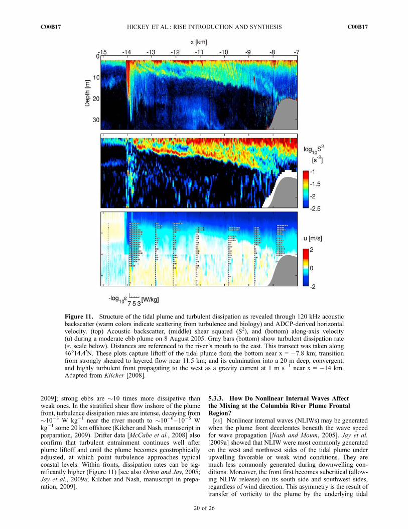
2009]; strong ebbs are �10 times more dissipative thanweak ones. In the stratified shear flow inshore of the plumefront, turbulence dissipation rates are intense, decaying from�10�3 W kg�1 near the river mouth to �10�6–10�5 Wkg�1 some 20 km offshore (Kilcher and Nash, manuscript inpreparation, 2009). Drifter data [McCabe et al., 2008] alsoconfirm that turbulent entrainment continues well afterplume liftoff and until the plume becomes geostrophicallyadjusted, at which point turbulence approaches typicalcoastal levels. Within fronts, dissipation rates can be sig-nificantly higher (Figure 11) [see also Orton and Jay, 2005;Jay et al., 2009a; Kilcher and Nash, manuscript in prepa-ration, 2009].

5.3.3. How Do Nonlinear Internal Waves Affectthe Mixing at the Columbia River Plume FrontalRegion?[68] Nonlinear internal waves (NLIWs) may be generated

when the plume front decelerates beneath the wave speedfor wave propagation [Nash and Moum, 2005]. Jay et al.[2009a] showed that NLIW were most commonly generatedon the west and northwest sides of the tidal plume underupwelling favorable or weak wind conditions. They aremuch less commonly generated during downwelling con-ditions. Moreover, the front first becomes subcritical (allow-ing NLIW release) on its south side and southwest sides,regardless of wind direction. This asymmetry is the result oftransfer of vorticity to the plume by the underlying tidal

Figure 11. Structure of the tidal plume and turbulent dissipation as revealed through 120 kHz acousticbackscatter (warm colors indicate scattering from turbulence and biology) and ADCP-derived horizontalvelocity. (top) Acoustic backscatter, (middle) shear squared (S2), and (bottom) along-axis velocity(u) during a moderate ebb plume on 8 August 2005. Gray bars (bottom) show turbulent dissipation rate(e, scale below). Distances are referenced to the river’s mouth to the east. This transect was taken along46�14.40N. These plots capture liftoff of the tidal plume from the bottom near x = �7.8 km; transitionfrom strongly sheared to layered flow near 11.5 km; and its culmination into a 20 m deep, convergent,and highly turbulent front propagating to the west as a gravity current at 1 m s�1 near x = �14 km.Adapted from Kilcher [2008].


20 of 26

C00B17

flow. Pan and Jay [2009] found that the ambient velocityshear alters the structure of the NLIW by displacing themaximum of the NLIW vertical structure function as muchas 5 m below the density interface. This greatly affectsNLIW-induced turbulent mixing at the frontal region,because the displaced maximum internal wave shear is ata depth with reduced stability, N2. An analysis based onobservations and internal wave theory suggests that thevertical velocity shear is intensified primarily by the inter-action between sheared ambient velocity and the NLIWvertical structure at depths where the combined NLIW andambient shears result in Rig�0.25. Typically, neither mech-anism acting alone would drive mixing.5.3.4. How, Where, and When are PhytoplanktonEntrained Into the Plume?[69] Based on the physical and chemical observations, it

is clear that most of the turbulent mixing in the plumeoccurs at the estuary bar and at the tidal plume front, oververy short time scales. There was no evidence for distinctplume phytoplankton communities [Frame and Lessard,2009], and no evidence for distinct physiological responsesin the plume versus outside the plume [Kudela and Peterson,2009]. This is consistent with the plume entraining andmixingphytoplankton from the near-field coastal waters; while theplume has strikingly different physical and chemical proper-ties, it acts more as biological capacitor (capturing nearshorecoastal waters and sometimes adding nutrients), rather thanserving as a distinct source or sink for phytoplankton.5.3.5. Does the Regional Plume Have MultiplePhysical, Chemical, or Biological Regions or LayersThat Can Be Distinguished?[70] The water properties of the Columbia plume, which

depend on the properties of both river and ocean end-members as well as the degree of mixing are extremelytime-variable as described above. Thus, it is difficult toascribe specific values of properties to the different plumeregions, such as the source region (from the estuary mouthto about 5 km upstream of the mouth), the tidal plume (thepulse of mixed river and shelf water discharged onto theshelf during a single ebb tide; e.g., Figure 11), or the agingplume waters (sometimes referred to as the ‘‘far-field’’plume). Nevertheless, property gradients are usually suffi-ciently large that the tidal plume can be readily distin-guished from aging plume waters or deep water that hasrecently upwelled. The tidal plume overlays preexisting oraging plume waters, producing visible layers of salinity,temperature, density and nutrients [Horner-Devine et al.,2009]. Although the estuarine source waters contain fresh-water phytoplankton species, because these rapidly die outon encountering oceanic waters, and are replaced by shelfspecies entrained during mixing, phytoplankton layers areless distinguishable. Significant differences in species com-position and diatom composition between plume andoceanic waters have been documented during some plumeevents [Frame and Lessard, 2009].[71] Although nitrate and much of the dissolved iron is

rapidly assimilated by plume phytoplankton, the largeexcess of these other chemicals in the plume can serveto distinguish the plume. For example, Aguilar-Islas andBruland [2006] demonstrated how elevated silicic acid anddissolved manganese could be used as chemical tracers ofthe far-field plume. Brown and Bruland [2009] showed how

elevated dissolved and particulate aluminum in theColumbia River plume could be followed hundreds of kmfrom the river mouth. The dissolved manganese in theColumbia River estuary varies dramatically as a functionof spring or neap tides [Aguilar-Islas and Bruland, 2006;Bruland et al., 2008]. This can be used to distinguish agedplumes that formed under spring tide conditions fromplumes that formed under neap tide conditions.

6. Conclusions

[72] RISE studies have resulted in the development of anew working model of plume processes (Figure 12). Thecartoon illustrating this model shows plume processes inplan view as well as along sections emanating from the rivermouth and downstream of the mouth. River and tidal waters(1–12 h) are differentiated from aging (1–10 d and up-welling (1–10 d) waters. The cartoon reflects the modernpicture of the Columbia plume: a plume with two branches,rather than simply a single southwest plume as depicted inthe historic literature [Hickey et al., 2005; Liu et al., 2009a].The northward branch of the Columbia plume in spring can,on occasion, transit the entire Washington shelf, wraparound the eddy offshore of the Strait of Juan de Fucaand return south to join newly emerging plume waters some10–20 d later [Hickey et al., 2009].[73] With respect to the three original RISE hypotheses

given in section 1, (1) primary production has been shownto be higher in the newly emerging plume waters than onshelves outside the plume (Figures 12a and 12b) and plumeturbidity does not appear to inhibit growth. (2) Modelstudies demonstrate that cross-shelf export is enhanced byabout 20% by the presence of the river plume (Figure 12c).Last, it has been shown that the area both north and south ofthe river mouth appear to be iron and silicate replete due tothe presence of the Columbia plume [Bruland et al., 2008];in particular, iron limitation on phytoplankton growth isunlikely and diatoms are almost always dominant [Kudelaet al., 2006; Frame and Lessard, 2009]. This result funda-mentally differentiates the northern CCS from coastalwaters in the more southern parts of the CCS. No north–south rate differences due to silicate or iron supply weredocumented.[74] A number of other important improvements in

understanding how freshwater mixes into the coastal oceanand how the resulting plume affects the local ecosystemhave emerged from RISE. For example, in situ measure-ments and model studies demonstrated where mixing occursand the magnitude of mixing rates, which decreasewith distance from the river mouth [Nash et al., 2009;MacCready et al., 2009]. Nonlinear internal waves, gener-ated on the west/northwest side of the plume under upwell-ing favorable or weak wind conditions (Figure 12c), alsoaffect mixing of plume water [Jay et al., 2009a]. About halfthe mixing occurs inside the estuary and near the mouth,with the remainder occurring primarily as a result of windmixing as the plume ages. Nitrate (during upwellingperiods) and plankton are both entrained into the plume inthe estuary and near mouth mixing; the plume in generaldoes not contain unique phytoplankton assemblages. Theriver itself can contribute nitrate to the plume with generallylow concentrations in summer, and higher concentrations in


21 of 26

C00B17

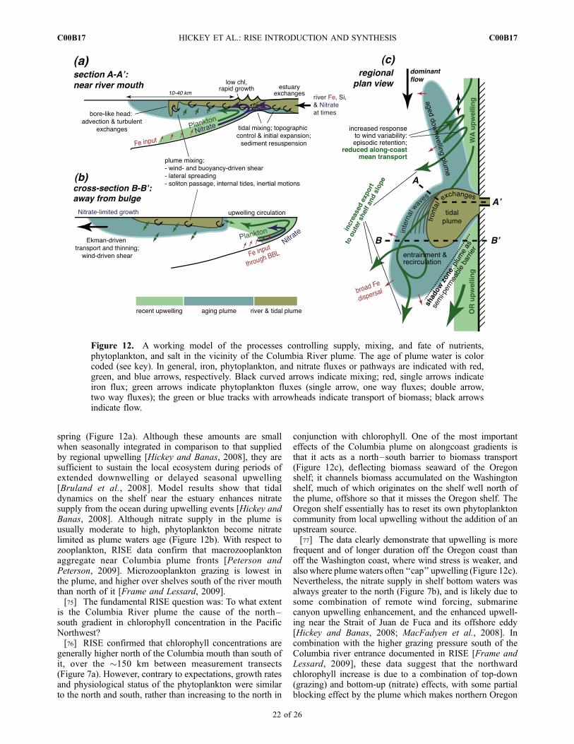
spring (Figure 12a). Although these amounts are smallwhen seasonally integrated in comparison to that suppliedby regional upwelling [Hickey and Banas, 2008], they aresufficient to sustain the local ecosystem during periods ofextended downwelling or delayed seasonal upwelling[Bruland et al., 2008]. Model results show that tidaldynamics on the shelf near the estuary enhances nitratesupply from the ocean during upwelling events [Hickey andBanas, 2008]. Although nitrate supply in the plume isusually moderate to high, phytoplankton become nitratelimited as plume waters age (Figure 12b). With respect tozooplankton, RISE data confirm that macrozooplanktonaggregate near Columbia plume fronts [Peterson andPeterson, 2009]. Microzooplankton grazing is lowest inthe plume, and higher over shelves south of the river mouththan north of it [Frame and Lessard, 2009].[75] The fundamental RISE question was: To what extent

is the Columbia River plume the cause of the north–south gradient in chlorophyll concentration in the PacificNorthwest?[76] RISE confirmed that chlorophyll concentrations are

generally higher north of the Columbia mouth than south ofit, over the �150 km between measurement transects(Figure 7a). However, contrary to expectations, growth ratesand physiological status of the phytoplankton were similarto the north and south, rather than increasing to the north in

conjunction with chlorophyll. One of the most importanteffects of the Columbia plume on alongcoast gradients isthat it acts as a north–south barrier to biomass transport(Figure 12c), deflecting biomass seaward of the Oregonshelf; it channels biomass accumulated on the Washingtonshelf, much of which originates on the shelf well north ofthe plume, offshore so that it misses the Oregon shelf. TheOregon shelf essentially has to reset its own phytoplanktoncommunity from local upwelling without the addition of anupstream source.[77] The data clearly demonstrate that upwelling is more

frequent and of longer duration off the Oregon coast thanoff the Washington coast, where wind stress is weaker, andalso where plumewaters often ‘‘cap’’ upwelling (Figure 12c).Nevertheless, the nitrate supply in shelf bottom waters wasalways greater to the north (Figure 7b), and is likely due tosome combination of remote wind forcing, submarinecanyon upwelling enhancement, and the enhanced upwell-ing near the Strait of Juan de Fuca and its offshore eddy[Hickey and Banas, 2008; MacFadyen et al., 2008]. Incombination with the higher grazing pressure south of theColumbia river entrance documented in RISE [Frame andLessard, 2009], these data suggest that the northwardchlorophyll increase is due to a combination of top-down(grazing) and bottom-up (nitrate) effects, with some partialblocking effect by the plume which makes northern Oregon

Figure 12. A working model of the processes controlling supply, mixing, and fate of nutrients,phytoplankton, and salt in the vicinity of the Columbia River plume. The age of plume water is colorcoded (see key). In general, iron, phytoplankton, and nitrate fluxes or pathways are indicated with red,green, and blue arrows, respectively. Black curved arrows indicate mixing; red, single arrows indicateiron flux; green arrows indicate phytoplankton fluxes (single arrow, one way fluxes; double arrow,two way fluxes); the green or blue tracks with arrowheads indicate transport of biomass; black arrowsindicate flow.


22 of 26

C00B17

a ‘‘shadow zone.’’ Although the spatial pattern of grazinglikely reflects the influence of the plume [Banas et al.,2009b], enhanced nitrate supply to the northern Washingtonshelf is not related to the plume.[78] Thus the Columbia plume does indeed appear to be

instrumental in making the southern Washington coast sucha rich ecosystem, both through increased nutrient supply orconsistency of supply, and increased retention of nutrientsand biomass; but the northern source of nutrients andbiomass appears to play just as significant a role.Accordingly, to allow quantitative comparison of theseprocesses, models and data collection must expand in scale,to encompass the interactions between freshwater inputsand retention features over hundreds of kilometers ofcoastline.

[79] Acknowledgments. This summary was supported by grantOCE-0239089 to B. Hickey, P. MacCready, and E. Lessard;OCE-0238347 to K. Bruland and R. Kudela; OCE-0238021 to E. Dever;OCE-0238727 to J. Nash and J. Moum; OCE-0237710 to M. Kosro;OCE-0622278 and OCE-0239072 to D. Jay and A. Baptista; andOCE-0239107 to W. Peterson from the National Science Foundation (NSF)as part of the Coastal Ocean Processes RISE Program. The CORIE/SATURNobservation and prediction system is scientific infrastructure of the NSFScience and Technology Center for Coastal Margin Observation and Predic-tion (OCE-0424602) and is also partially supported by regional stakeholders,including the National Oceanic and Atmospheric Administration and theBonneville Power Administration. The authors would like to thank thecaptains and crews of the R/V Wecoma and Pt. Sur for their outstandingsupport of this research. RISE would not have been successful without thecombined efforts of numerous staff and students from each of the researchteams; in particular, Nancy Kachel, Susan Geier, Mike Foy, MeganBernhardt, David Darr, Sherry Palacios, Misty Blakely, Bettina Sohst,Geoffrey Smith, and Keith Leffler. This is contribution 48 of the RISEprogram. The statements, findings, conclusions, and recommendations arethose of the authors and do not necessarily reflect the views of NSF.

ReferencesAguilar-Islas, A. M., and K. W. Bruland (2006), Dissolved manganese andsilicic acid in the Columbia River plume: A major source to the Californiacurrent and coastal waters off Washington and Oregon, Mar. Chem.,101(3–4), 233–247, doi:10.1016/j.marchem.2006.03.005.

Bakun, A. (1973), Coastal upwelling indices, west coast of North America,1946–71, NOAA Tech. Rep. NMFS SSRF-671, 103 pp., U.S. Dep. ofCommer., Washington, D. C.

Banas, N. S., P. MacCready, and B. M. Hickey (2009a), The ColumbiaRiver plume as cross-shelf exporter and along-coast barrier, Cont. ShelfRes., 29(1), 292–301, doi:10.1016/j.csr.2008.03.011.

Banas, N. S., E. J. Lessard, R. M. Kudela, P. MacCready, T. D. Peterson,B. M. Hickey, and E. Frame (2009b), Planktonic growth and grazing inthe Columbia River plume region: A biophysical model study, J. Geo-phys. Res., 114, C00B06, doi:10.1029/2008JC004993.

Baptista, A. M. (2006), CORIE: The first decade of a coastal-margincollaborative observatory, in Oceans 2006, pp. 1–6, Inst. of Electr. andElectr. Eng., Boston.

Baptista, A. M., Y. Zhang, A. Chawla, M. Zulauf, C. Seaton, E. P. Myers,J. Kindle, M. Wilkin, M. Burla, and P. J. Turner (2005), A cross-scalemodel for 3D baroclinic circulation in estuary-plume-shelf systems: II.Application to the Columbia River, Cont. Shelf Res., 25, 935–972,doi:10.1016/j.csr.2004.12.003.

Barnes, C. A., A. C. Duxbury, and B. A. Morse (1972), Circulation andselected properties of the Columbia River effluent at sea, in The ColumbiaRiver Estuary and Adjacent OceanWaters, edited by A. T. Pruter and D. L.Alverson, pp. 41–80, Univ. of Wash. Press, Seattle, Wash.

Barron, C. N., A. B. Kara, P. J. Martin, R. C. Rhodes, and L. F. Smedstad(2006), Formulation, implementation and examination of vertical coordinatechoices in the global Navy Coastal Ocean Model (NCOM), Ocean Modell.,11(3–4), 347–375, doi:10.1016/j.ocemod.2005.01.004.

Battisti, D., and B. M. Hickey (1984), Application of remote wind forcedcoastal trapped wave theory to the Oregon and Washington coasts,J. Phys. Oceanogr., 14, 887–903, doi:10.1175/1520-0485(1984)014<0887:AORWFC>2.0.CO;2.

Bi, H., R. E. Ruppel, and W. T. Peterson (2007), Modeling the salmonpelagic habitat off the Pacific Northwest (USA) coast using logistic

regression, Mar. Ecol. Prog. Ser., 336, 249 – 265, doi:10.3354/meps336249.

Boicourt, W. C., W. J. Wiseman Jr., A. Valle-Levinson, and L. P. Atkinson(1998), Continental shelf of the southeastern United States and the Gulfof Mexico: In the shadow of the Western Boundary Current, in The Sea,vol. 11, edited by A. R. Robinson and K. H. Brink, pp. 135–182, JohnWiley, New York.

Bottom, D. L., C. A. Simenstad, J. Burke, A. M. Baptista, D. A. Jay,K. K. Jones, E. Casillas, and M. H. Schiewe (2005), Salmon at river’s end:The role of the estuary in the decline and recovery of Columbia Riversalmon, NOAA Tech. Memo., NMFS-NWFSC-68, 246 pp., U.S. Dep. ofCommer., Washington, D. C.

Brown, M. T., and K. W. Bruland (2009), Dissolved and particulatealuminum in the Columbia River and coastal waters of Oregon andWashington: Behavior in near-field and far-field plumes, EstuarineCoastal Shelf Sci., 84, 171–185, doi:10.1016/j.ecss.2009.05.031.

Bruland, K. W., E. L. Rue, and G. J. Smith (2001), Iron and macronutrientsin California coastal upwelling regimes: Implications for diatom blooms,Limnol. Oceanogr., 46, 1661–1674.

Bruland, K. W., M. C. Lohan, A. M. Aguilar-Islas, G. J. Smith, B. Sohst,and A. Baptista (2008), Factors influencing the chemistry and formationof the Columbia River plume: Nitrate, silicic acid, dissolved Fe anddissolved Mn, J. Geophys. Res., 113 , C00B02, doi:10.1029/2007JC004702.

Burla, M., A. M. Baptista, Y. Zhang, and S. Frolov (2009), Seasonal andinterannual variability of the Columbia River plume: A perspectiveenabled by multiyear simulation databases, J. Geophys. Res.,doi:10.1029/2008JC004964, in press.

Chao, S.-Y., and W. C. Boicourt (1986), Onset of estuarine plumes, J. Phys.Oceanogr., 16, 2137 – 2149, doi:10.1175/1520-0485(1986)016<2137:OOEP>2.0.CO;2.

Chase, Z., A. van Geen, P. M. Kosro, J. Marra, and P. A. Wheeler (2002),Iron, nutrient, and phytoplankton distributions in Oregon coastal waters,J. Geophys. Res., 107(C10), 3174, doi:10.1029/2001JC000987.

Chase, Z., P. Strutton, and B. Hales (2007), Iron links river runoff and shelfwidth to phytoplankton biomass along the U.S. West Coast, Geophys.Res. Lett., 34, L04607, doi:10.1029/2006GL028069.

Chawla, A., D. A. Jay, A. M. Baptista, M. Wilkin, and C. Seaton (2008),Seasonal variability and estuary-shelf interactions in circulation dynamicsof a river-dominated estuary, Estuaries Coasts, 31, 269 – 288,doi:10.1007/s12237-007-9022-7.

Conomos, T. J., M. G. Gross, C. A. Barnes, and F. A. Richards (1972),River-ocean nutrient relations in summer, in The Columbia River Estuaryand Adjacent Ocean Waters, edited by A. T. Pruter and D. L. Alverson,pp. 151–175, Univ. of Wash. Press, Seattle, Wash.

Cudaback, C. N., and D. A. Jay (2000), Tidal asymmetry in an estuarinepycnocline: Depth and thickness, J. Geophys. Res., 105, 26,237–26,252,doi:10.1029/2000JC900135.

Cudaback, C. N., and D. A. Jay (2001), Tidal asymmetry in an estuarinepycnocline: 2. Transport, J. Geophys. Res., 106(C2), 2639 – 2652,doi:10.1029/2000JC900151.

Dracup, J. A., and E. Kahya (1994), The relationships between U.S. stream-flow and La Nina events, Water Resour. Res., 30, 2133 – 2141,doi:10.1029/94WR00751.

Fain, A. M. V., D. A. Jay, D. J. Wilson, P. M. Orton, and A. M. Baptista(2001), Seasonal, monthly and tidal patterns of particulate matterdynamics in the Columbia River estuary, Estuaries Coasts, 24, 770–786, doi:10.2307/1352884.

Firme, G. F., E. L. Rue, D. A. Weeks, K. W. Bruland, and D. A. Hutchins(2003), Spatial and temporal variability in phytoplankton iron limitationalong the California coast and consequences for Si, N and C biogeochemistry,Global Biogeochem. Cycles, 17(1), 1016, doi:10.1029/2001GB001824.

Fischer, H. B. (1972), Mass transport mechanisms in partially stratifiedes tuar ies , J . Flu id Mech. , 53 (4) , 671 – 687, doi :10 .1017/S0022112072000412.

Fong, D., and W. R. Geyer (2002), The alongshore transport of fresh waterin a surface-trapped river plume, J. Phys. Oceanogr., 32(3), 957–972,doi:10.1175/1520-0485(2002)032<0957:TATOFI>2.0.CO;2.

Frame, E. R., and E. J. Lessard (2009), Does the Columbia River plumeinfluence phytoplankton community structure along the Washington andOregon coasts?, J. Geophys. Res., 114, C00B09, doi:10.1029/2008JC004999.

Friedrichs, M. A. M., et al. (2007), Assessment of skill and portability inregional marine biogeochemical models: Role of multiple planktonicgroups, J. Geophys. Res., 112, C08001, doi:10.1029/2006JC003852.

Frolov, S., A. M. Baptista, and M. Wilkin (2008), Optimizing fixedobservational assets in a coastal observatory, Cont. Shelf Res., 28(19),2644–2658, doi:10.1016/j.csr.2008.08.009.

Frolov, S., A. M. Baptista, T. Leen, Z. Lu, and R. van der Merwe (2009a),Fast data assimilation using a nonlinear Kalman filter and a model


23 of 26

C00B17

surrogate: An application to the Columbia River estuary, Dyn. Atmos.Oceans, 48, 16–45, doi:10.1016/jdynatmoce.2008.10.004.

Frolov, S., A. M. Baptista, Y. Zhang, and C. Seaton (2009b), Estimation ofecologically significant circulation features of the Columbia River estuaryand plume using a reduced-dimension Kalman filter, Cont. Shelf Res.,29(2), 456–466, doi:10.1016/j.csr.2008.11.004.

Garcia-Berdeal, I., B. M. Hickey, and M. Kawase (2002), Influence of windstress and ambient flow on a high discharge river plume, J. Geophys.Res., 107(C9), 3130, doi:10.1029/2001JC000932.

Garvine, R. W. (1982), A steady state model for buoyant surface plumehydrodynamics in coastal waters, Tellus, 34, 293–306.

Garvine, R. W. (1999), Penetration of buoyant coastal discharge onto thecontinental shelf: A numerical model experiment, J. Phys. Oceanogr., 29,1892–1909, doi:10.1175/1520-0485(1999)029<1892:POBCDO>2.0.CO;2.

Gershunov, A., T. P. Barnett, and D. R. Cayan (1999), North Pacificinterdecadal oscillation seen as factor in ENSO-related North Americanclimate anomalies, Eos Trans. AGU, 80(3), 25, doi:10.1029/99EO00019.

Giese, B. S., and D. A. Jay (1989), Modeling tidal energetics of theColumbia River estuary, Estuarine Coastal Shelf Sci., 29(6), 549–571,doi:10.1016/0272-7714(89)90010-3.

Hamilton, P. (1990), Modeling salinity and circulation for the ColumbiaRiver estuary, Prog. Oceanogr., 25(1–4), 113–156, doi:10.1016/0079-6611(90)90005-M.

Hickey, B. M. (1979), The California current system—Hypotheses andfacts, Prog. Oceanogr., 8, 191–279, doi:10.1016/0079-6611(79)90002-8.

Hickey, B. M. (1989), Patterns and processes of shelf and slope circulation,in Coastal Oceanography of Washington and Oregon, edited by M. R.Landry and B. M. Hickey, pp. 41–115, Elsevier Sci., Amsterdam.

Hickey, B. M. (1998), Coastal oceanography of western North Americafrom the tip of Baja California to Vancouver Is, in The Sea, vol. 11,edited by K. H. Brink and A. R. Robinson, pp. 345–393, John Wiley,New York.

Hickey, B. M., and N. Banas (2003), Oceanography of the Pacific North-west coastal ocean and estuaries with application to coastal ecosystems,Estuaries Coasts, 26(48), 1010–1031.

Hickey, B. M., and N. Banas (2008), Why is the northern California Currentso Productive?, Oceanography, 21(4), 90–107.

Hickey, B. M., L. J. Pietrafesa, D. A. Jay, and W. C. Boicourt (1998), TheColumbia River plume study: Subtidal variability in the velocity andsalinity fields, J. Geophys. Res., 103, 10,339–10,368, doi:10.1029/97JC03290.

Hickey, B. M., S. Geier, N. Kachel, and A. MacFadyen (2005), Abi-directional river plume: The Columbia in summer, Cont. Shelf Res.,25(14), 1631–1656, doi:10.1016/j.csr.2005.04.010.

Hickey, B. M., A. MacFadyen, W. P. Cochlan, R. M. Kudela, K. W.Bruland, and C. R. Trick (2006), Evolution of biological, chemicaland physical water properties in the Pacific Northwest in 2005: Remoteor local wind forcing?, Geophys. Res. Lett., 33, L22S02, doi:10.1029/2006GL026782.

Hickey, B. M., R. McCabe, S. Geier, E. Dever, and N. Kachel (2009), Threeinteracting freshwater plumes in the northern California Current System,J. Geophys. Res., 114, C00B03, doi:10.1029/2008JC004907.

Hooff, R. C., and W. T. Peterson (2006), Recent increases in copepodbiodiversity as an indicator of changes in ocean and climate conditionsin the northern California Current ecosystem, Limnol. Oceanogr., 51,2042–2051.

Horner-Devine, A. R. (2009), The bulge circulation in the Columbia Riverplume, Cont. Shelf Res., 29(1), 234–251, doi:10.1016/j.csr.2007.12.012.

Horner-Devine, A., D. Fong, S. Monismith, and T. Maxworthy (2006),Laboratory experiments simulating a coastal river inflow, J. Fluid Mech.,555, 203–232, doi:10.1017/S0022112006008937.

Horner-Devine, A. R., D. A. Jay, P. M. Orton, and E. Spahn (2009), Aconceptual model of the strongly tidal Columbia River plume, J. Mar.Syst., 78, 460–475, doi:10.1016/j.jmarsys.2008.11.025.

Hughes, R. P., and M. Rattray (1980), Salt flux and mixing in the ColumbiaRiver estuary, Estuarine Coastal Mar. Sci., 10, 479–494, doi:10.1016/S0302-3524(80)80070-3.

Hutchins, D. A., and K. W. Bruland (1998), Iron-limited diatom growth andSi:N uptake ratios in a coastal upwelling regime, Nature, 393, 561–564,doi:10.1038/31203.

Hutchins, D. A., G. R. DiTullio, Y. Zhang, and K. W. Bruland (1998),An iron limitation mosaic in the California upwelling regime, Limnol.Oceanogr., 43, 1037–1054.

Huyer, A., E. J. C. Sobey, and R. L. Smith (1979), The spring transition incurrents over the Oregon continental shelf, J. Geophys. Res., 84(C11),6995–7011, doi:10.1029/JC084iC11p06995.

Jay, D. A., and J. D. Musiak (1996), Internal tidal asymmetry in channelflows: Origins and consequences, inMixing in Estuaries and Coastal Seas,

Coastal Estuarine Stud., vol. 50, edited by C. Pattiaratchi, pp. 219–258,AGU,Washington, D. C.

Jay, D. A., and J. D. Smith (1990a), Circulation, density distribution andneap-spring transitions in the Columbia River estuary, Prog. Oceanogr.,25, 81–112, doi:10.1016/0079-6611(90)90004-L.

Jay, D. A., and J. D. Smith (1990b), Residual circulation in shallowestuaries: 1. Highly stratified, narrow estuaries, J. Geophys. Res.,95(C1), 711–731, doi:10.1029/JC095iC01p00711.

Jay, D. A., and J. D. Smith (1990c), Residual circulation in shallowestuaries: 2. Weakly stratified and partially mixed, narrow estuaries,J. Geophys. Res., 95(C1), 733–748, doi:10.1029/JC095iC01p00733.

Jay, D. A., J. Pan, P. M. Orton, and A. Horner-Devine (2009a), Asymmetryof Columbia River tidal plume fronts, J. Mar. Syst., 78, 442–459,doi:10.1016/j.jmarsys.2008.11.015.

Jay, D. A., E. D. Zaron, and J. Pan (2009b), Initial expansion of the ColumbiaRiver tidal plume, J. Geophys. Res., doi:10.1029/2008JC004996, in press.

Kay, D. J., and D. A. Jay (2003a), Interfacial mixing in a highly stratifiedestuary: 1. Characteristics of mixing, J. Geophys. Res., 108(C3), 3072,doi:10.1029/2000JC000252.

Kay, D. J., and D. A. Jay (2003b), Interfacial mixing in a highly stratifiedestuary: 2. A ‘‘method of constrained differences’’ approach for thedetermination of the momentum and mass balances and the energy ofmixing, J. Geophys. Res., 108(C3), 3073, doi:10.1029/2000JC000253.

Kilcher, L. (2008), Turbulence in river plumes, Oceanography, 21(4), 31.Kosro, P. M. (2005), On the spatial structure of coastal circulationoff Newport, Oregon, during spring and summer 2001, in a region ofvarying shelf width, J. Geophys. Res., 110, C10S06, doi:10.1029/2004JC002769.

Kosro, P. M., W. T. Peterson, B. M. Hickey, R. K. Shearmann, and S. D.Pierce (2006), Physical versus biological spring transition, Geophys. Res.Lett., 33, L22S03, doi:10.1029/2006GL027072.

Kudela, R. M., and T. D. Peterson (2009), Influence of a buoyant riverplume on phytoplankton nutrient dynamics: What controls standingstocks and productivity?, J. Geophys. Res., 114, C00B11, doi:10.1029/2008JC004913.

Kudela, R. M., W. Cochlan, T. Peterson, and C. Trick (2006), Impacts onphytoplankton biomass and productivity in the Pacific Northwest duringthe warm ocean conditions of 2005, Geophys. Res. Lett., 33, L22S06,doi:10.1029/2006GL026772.

Landry, M. R., and B. M. Hickey (1989), Coastal Oceanography ofWashington and Oregon, 607 pp., Elsevier Sci., Amsterdam.

Landry, M. R., and C. J. Lorenzen (1989), Abundance, distribution, andgrazing impact of zooplankton on the Washington shelf, in CoastalOceanography of Washington and Oregon, edited by M. R. Landryand B. M. Hickey, pp. 175–202, Elsevier Sci., Amsterdam.

Landry, M. R., J. R. Postel, W. K. Peterson, and J. Newman (1989), Broad-scale distributional patterns of hydrographic variables on the Washington/Oregon shelf, in Coastal Oceanography of Washington and Oregon,edited by M. R. Landry and B. M. Hickey, pp. 1–40, Elsevier Sci.,Amsterdam.

Legaard, K. R., and A. C. Thomas (2006), Spatial patterns in seasonal andinterannual variability of chlorophyll and sea surface temperature in theCalifornia Current, J. Geophys. Res., 111, C06032, doi:10.1029/2005JC003282.

Lessard, E. J., and E. R. Frame (2008), The influence of the ColumbiaRiver plume on patterns of phytoplankton growth, grazing and chloro-phyll on the Washington and Oregon coasts, paper presented at 2008Ocean Sciences Meeting, Am. Soc. of Limnol. Oceanogr., Orlando,Fla., 2–7 March.

Li, M., L. Zhong, and W. C. Boicourt (2005), Simulations of ChesapeakeBay estuary: Sensitivity to turbulence mixing parameterizations andcomparison with observations, J. Geophys. Res., 110, C12004,doi:10.1029/2004JC002585.

Liu, Y., P. MacCready, and B. M. Hickey (2009a), Columbia River plumepatterns as revealed by a hindcast coastal ocean circulation model insummer 2004, Geophys. Res. Lett., 36, L02601, doi:10.1029/2008GL036447.

Liu, Y., P. MacCready, B. M. Hickey, E. P. Dever, P. M. Kosro, and N. S.Banas (2009b), Evaluation of a coastal ocean circulation model for theColumbia River plume in summer 2004, J. Geophys. Res., 114, C00B04,doi:10.1029/2008JC004929.

Lohan, M. C., and K. W. Bruland (2006), Importance of vertical mixing foradditional sources or nitrate and iron to surfaces waters of the ColumbiaRiver plume: Implications for biology, Mar. Chem., 98, 260 –273,doi:10.1016/j.marchem.2005.10.003.

Lohan, M. C., and K. W. Bruland (2008), Elevated Fe (II) and totaldissolved Fe in hypoxic shelf waters off the coast of Washington andOregon: An enhanced source of iron to coastal upwelling regimes,Environ. Sci. Technol., 42(17), 6462–6468, doi:10.1021/es800144j.


24 of 26

C00B17

Lohrenz, S. E., G. L. Fahnenstiel, D. F. Millie, O. M. E. Schofield,T. Johengen, and T. Bergmann (2004), Spring phytoplankton photosynthesis,growth, and primary production and relationships to a recurrent sedimentplume and river inputs in southeastern Lake Michigan, J. Geophys. Res.,109, C10S14, doi:10.1029/2004JC002383.

MacCready, P., N. S. Banas, B. M. Hickey, E. P. Dever, and Y. Liu (2009),A model study of tide- and wind-induced mixing in the Columbia Riverestuary and plume, Cont. Shelf Res., 29(1), 278–291, doi:10.1016/j.csr.2008.03.015.

MacFadyen, A., B. M. Hickey, and M. G. G. Foreman (2005), Transport ofsurface waters from the Juan de Fuca Eddy region to the Washingtoncoast: Implications for HABs, Cont. Shelf Res., 25, 2008 – 2021,doi:10.1016/j.csr.2005.07.005.

MacFadyen, A., B. M. Hickey, and W. P. Cochlan (2008), Influences of theJuan de Fuca Eddy on circulation, nutrients, and phytoplankton produc-tion in the northern California Current System, J. Geophys. Res., 113,C08008, doi:10.1029/2007JC004412.

Mantua, N. J., S. R. Hare, Y. Zhang, J. M. Wallace, and R. C. Francis(1997), A Pacific interdecadal climate oscillation with impacts on salmonproduction, Bull. Am. Meteorol. Soc., 78, 1069–1079, doi:10.1175/1520-0477(1997)078<1069:APICOW>2.0.CO;2.

Mass, C., et al. (2003), Regional environmental prediction over the PacificNorthwest, Bull. Am. Meteorol. Soc., 84, 1353–1366, doi:10.1175/BAMS-84-10-1353.

McCabe, R., B. Hickey, and P. MacCready (2008), Observational estimatesof entrainment and vertical salt flux behind the frontal boundary of aspreading river plume, J. Geophys. Res., 113, C08027, doi:10.1029/2007JC004361.

McCabe, R. M., P. MacCready, and B. M. Hickey (2009), Ebb tide dynamicsand spreading of a large river plume, J. Phys. Oceanogr., 39, 2839–2856,doi:10.1175/2009JPO4061.1.

Morgan, C. A., A. De Robertis, and R. W. Zabel (2005), Columbia Riverplume fronts: I. Hydrography, zooplankton distribution, and communitycomposition, Mar. Ecol. Prog. Ser., 299, 19 – 31, doi:10.3354/meps299019.

Nash, J. D., and J. N. Moum (2005), River plumes as a source of large-amplitude internal waves in the coastal ocean, Nature, 437, 400–403,doi:10.1038/nature03936.

Nash, J. D., L. Kilcher, and J. N. Moum (2009), Structure and compositionof a strongly stratified, tidally pulsed river plume, J. Geophys. Res., 114,C00B12, doi:10.1029/2008JC005036.

Nittrouer, C. A. (1978), The process of detrital sediment accumulation in acontinental shelf environment: An examination of the Washington shelf,Ph.D. dissertation, 243 pp., Univ. of Washington, Seattle, Wash.

Orton, P. M., and D. A. Jay (2005), Observations at the tidal plume front ofa high volume river outflow, Geophys. Res. Lett., 32, L11605,doi:10.1029/2005GL022372.

Pan, J., and D. A. Jay (2009), Effects of ambient velocity shear on internalsolitons and associated mixing at the Columbia River front, J. Geophys.Res., 114, C00B07, doi:10.1029/2008JC004988.

Pearcy, W. G. (1992), Books in Recruitment Fishery Oceanography: OceanEcology of North Pacific Salmonids, 179 pp., Univ. of Wash. Press,Seattle, Wash.

Peterson, J. O., and W. T. Peterson (2008), Influence of the Columbia Riverplume (USA) on the vertical and horizontal distribution of mesozooplanktonover the Washington and Oregon shelf, ICES J. Mar. Sci., 65, 477–483,doi:10.1093/icesjms/fsn006.

Peterson, J. O., and W. T. Peterson (2009), The influence of the ColumbiaRiver plume on cross-shelf transport of zooplankton, J. Geophys. Res.,114, C00B10, doi:10.1029/2008JC004965.

Pierce, D. P., J. A. Barth, R. E. Thomas, and G. W. Fleischer (2006),Anomalously warm July 2005 in the northern California Current: Historicalcontext and the significance of cumulative wind stress, Geophys. Res. Lett.,33, L22S04, doi:10.1029/2006GL027149.

Pruter, A. T., and D. L. Alverson (1972), The Columbia River Estuary andAdjacent Coastal Waters, 868 pp., Univ. of Wash. Press, Seattle, Wash.

Roegner, C., B. M. Hickey, J. Newton, A. Shanks, and D. Armstrong(2002), Estuarine-nearshore links during a coastal upwelling cycle:Plume and bloom intrusions into Willapa Bay, Washington, Limnol.Oceanogr., 47(4), 1033–1042.

Shaw, T. C., L. R. Feinberg, and W. T. Peterson (2009), Interannual varia-tions in vital rates of copepods and euphausiids during the RISE study2004 – 2006, J. Geophys. Res. , 114 , C00B08, doi:10.1029/2008JC004826.

Shulman, I., J. C. Kindle, S. deRada, S. C. Anderson, B. Penta, and P. J.Martin (2004), Development of a hierarchy of nested models to studythe California Current System, in Estuarine and Coastal Modeling:Proceedings of 8th International Conference on Estuarine and CoastalModeling, edited by M. L. Spaulding, pp. 74–88, Am. Soc. of Civ. Eng.,Reston, Va.

Simenstad, C. A., L. Small, C. D. McIntire, D. A. Jay, and C. R. Sherwood(1990a), Columbia River estuary studies: An introduction to the estuary, abrief history, and prior studies, Prog. Oceanogr., 25, 1–14, doi:10.1016/0079-6611(90)90002-J.

Simenstad, C. A., C. D. McIntire, and L. F. Small (1990b), Consumptionprocesses and food web structure in the Columbia River estuary, Prog.Oceanogr., 25, 271–298, doi:10.1016/0079-6611(90)90010-Y.

Small, L. F., C. D. McIntire, K. B. Macdonald, J. R. Laralara, B. E. Frey,M. C. Amspoker, and T. Winfield (1990), Primary production, plant anddetrital biomass, and particle transport in the Columbia River estuary,Prog. Oceanogr., 25, 175–210, doi:10.1016/0079-6611(90)90007-O.

Spahn, E. Y., A. R. Horner-Devine, D. A. Jay, J. Nash, and L. Kilcher(2009), Particle re-suspension in the Columbia River plume near field,J. Geophys. Res., 114, C00B14, doi:10.1029/2008JC004986.

Strub, P. T., J. S. Allen, A. Huyer, and R. L. Smith (1987), Large-scalestructure of the spring transition in the coastal ocean off western NorthAmerica, J. Geophys. Res., 92(C2), 1527 – 1544, doi:10.1029/JC092iC02p01527.

Strub, P. T., C. James, A. C. Thomas, and M. R. Abbott (1990), Seasonaland nonseasonal variability of satellite-derived surface pigment concen-tration in the California Current, J. Geophys. Res., 95, 11,501–11,530,doi:10.1029/JC095iC07p11501.

Sullivan, B. E., F. G. Prahl, L. F. Small, and P. A. Covert (2001),Seasonality of phytoplankton production in the Columbia River: Anatural or anthropogenic pattern?, Geochim. Cosmochim. Acta, 65,1125–1139, doi:10.1016/S0016-7037(00)00565-2.

Swartzman, G. L. (2001), Spatial patterns of hake (merluccius productus)shoals and euphausiid patches in the California current ecosystem, inSpatial Processes and Management of Marine Populations, edited byG. H. Kruse et al., pp. 495–512, Univ. of Alaska Sea Grant CollegeProgram, Fairbanks, Alaska.

Swartzman, G., and B. Hickey (2003), Evidence for a regime shift after the1997–1998 El Nino, based on 1995, 1998 and 2001 acoustic surveys inthe Pacific Eastern Boundary Current, Estuaries, 26(4), 1032–1043,doi:10.1007/BF02803361.

Thomas, A. C., and R. Weatherbee (2006), Satellite-measured temporalvariability of the Columbia River plume, Remote Sens. Environ., 100,167–178, doi:10.1016/j.rse.2005.10.018.

Thomas, A. C., M. E. Carr, and P. T. Strub (2001), Chlorophyll variabilityin eastern boundary Currents, Geophys. Res. Lett., 28, 3421–3424,doi:10.1029/2001GL013368.

Venegas, R., P. Strub, E. Beier, R. Letelier, A. Thomas, T. Cowles, C. James,L. Soto-Mardones, and C. Cabrera (2008), Satellite-derived variability inchlorophyll, wind stress, sea surface height, and temperature in the northernCalifornia Current system, J. Geophys. Res., 113, C03015, doi:10.1029/2007JC004481.

Ware, D. M., and R. E. Thomson (2005), Bottom-up ecosystem trophicdynamics determine fish production in the Northeast Pacific, Science,308(5726), 1280–1284, doi:10.1126/science.1109049.

Warner, J. C., W. R. Geyer, and J. A. Lerczak (2005), Numerical modelingof an estuary: A comprehensive skill assessment, J. Geophys. Res., 110,C05001, doi:10.1029/2004JC002691.

Wiseman, W. J., and R. W. Garvine (1995), Plumes and coastal currentsnear large river mouths, Estuaries Coasts, 18(3), 509–517, doi:10.2307/1352368.

Wolter, K., and M. S. Timlin (1993), Monitoring ENSO in COADS with aseasonally adjusted principal component index, paper presented at 17thClimate Diagnostics Workshop, NOAA, Norman, Okla.

Yankovsky, A. E., B. M. Hickey, and A. K. Munchow (2001), Impact ofvariable inflow on the dynamics of a coastal buoyant plume, J. Geophys.Res., 106, 19,809–19,824, doi:10.1029/2001JC000792.

Zhang, Y., and A. M. Baptista (2008), SELFE: A semi-implicit Eulerian-Lagrangian finite-element model for cross-scale ocean circulation, OceanModell., 21(3–4), 71–96, doi:10.1016/j.ocemod.2007.11.005.

Zhang, Y., A. M. Baptista, and E. P. Myers (2004), A cross-scale model for3D baroclinic circulation in estuary-plume-shelf systems: I. Formulationand skill assessment, Cont. Shelf Res., 24(18), 2187–2214, doi:10.1016/j.csr.2004.07.021.

��N. S. Banas, Applied Physics Laboratory, University of Washington,

Seattle, WA 98195, USA.A. M. Baptista, Science and Technology Center for Coastal Margin

Observation and Prediction, Oregon Health and Science University,Beaverton, OR 97006, USA.K. W. Bruland and R. M. Kudela, Department of Ocean Sciences,

University of California, Santa Cruz, CA 95064, USA.E. P. Dever, L. K. Kilcher, P. M. Kosro, J. D. Nash, and J. O. Peterson,

College of Ocean and Atmospheric Sciences, Oregon State University,Corvallis, OR 97331, USA.


25 of 26

C00B17

B. M. Hickey, E. J. Lessard, and P. MacCready, School of Oceanography,University of Washington, Seattle, WA 98195, USA. ([email protected])A. R. Horner-Devine, Civil and Environmental Engineering, University

of Washington, Seattle, WA 98195, USA.D. A. Jay, J. Pan, and E. D. Zaron, Civil and Environmental Engineering,

Portland State University, Portland, OR 97207, USA.

M. C. Lohan, SEOS, University of Plymouth, Plymouth, UK.R. M. McCabe, Department of Aviation, University of New South Wales,

Sydney, NSW 2052, Australia.P. M. Orton, Lamont-Doherty Earth Observatory, Earth Institute at

Columbia University, Palisades, NY 10964, USA.W. T. Peterson, Northwest Fisheries Science Center, NOAA Fisheries,

Newport, OR 97365, USA.


26 of 26

C00B17

Documents

River Influences on Shelf Ecosystems: Introduction and