Embed Size (px)
Citation preview

Background
!
Much excitement over RNA-Sequencing
Time
Excitement
RNA Sequencing
Microarrays
!
Measuring Gene Expression
Cell
Hybridize to arrayFragment
Sequence and countMeasure intensity

!
Data from D. melanogaster:chrX
Conservation
d_simulansd_sechelliad_yakubad_erectad_ananassaed_pseudoobscurad_persimilisd_willistonid_virilisd_mojavensisd_grimshawia_gambiaea_melliferat_castaneum
1067300010673500106740001067450010675000106755001067600010676500106770001067750010678000106785001067900010679500106800001068050010681000CG8144_6lane_0MM
S2_DRSC_6_lanes
FlyBase Protein-Coding Genes
RefSeq Genes
12 Flies, Mosquito, Honeybee, Beetle Multiz Alignments & phastCons Scores
Repeating Elements by RepeatMasker
CG15211CG15211CG15211CG15211
Ant2Ant2
sesBsesBsesBsesB
CG15211CG15211CG15211CG15211
Ant2Ant2
sesBsesBsesBsesB
_ 1000
_ 0
_ 1000
_ 0
ps RNAi
S2 Untreated
Splice JunctionReads
GenomicReads
Splice JunctionReads
GenomicReads
Image from Brenton Gravely
!
Why the excitement?
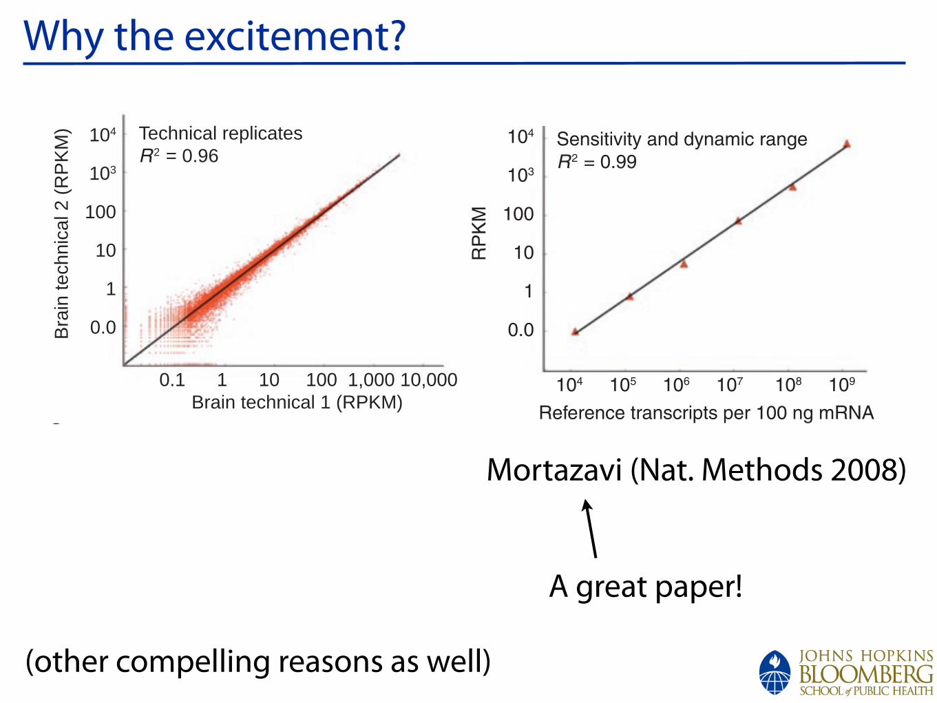
and phage lambda templates (Fig. 2c). These standards comprised long (~10,000 nt), intermediate (~1,500 nt) and short (~300 nt) transcripts, and they were designed to span the range of abundance (~0.5–50,000 transcripts per cell) typically observed in natural transcriptomes. RNA-Seq data for the standards were linear across a dynamic range of five orders of magnitude in RNA concentra-tion. Sequence coverage over test transcripts was highly reproducible and quite uniform (Supplementary Fig. 1c). At current practical sequencing capacity and cost (~40 M mapped reads), transcript detection was robust at 1.0 RPKM and above for a typical 2-kilo-base (kb) mRNA (~80 individual sequence reads resulting in a P value <10 16). Beyond simple detection confidence, we analyzed the impact of different amounts of sequencing on our ability to measure the concentration of a given transcript class (defined on the basis of RPKM) within ±5% (Fig. 2d). When these RNA standards are used in conjunction with information on cellular RNA content, abso-lute transcript levels per cell can also be calculated. For example, on the basis of literature values for the mRNA content of a liver cell19 and the RNA standards, we estimated that 3 RPKM corresponds to about one transcript per liver cell. For C2C12 tissue culture cells, for
High read number is relevant for RNA-Seq because our ability to reliably detect and measure rare, yet physiologically relevant, RNA species (those with abundances of 1–10 RNAs per cell) depends on the number of independent pieces of evidence (sequence reads) obtained for transcripts from each gene. This constraint influenced our sequencing strategy, choice of instrument and choice of the 25-bp read length.
The sensitivity of RNA-Seq will be a function of both molar con-centration and transcript length. We therefore quantified transcript levels in reads per kilobase of exon model per million mapped reads (RPKM) (Fig. 1a,c). The RPKM measure of read density reflects the molar concentration of a transcript in the starting sample by normalizing for RNA length and for the total read number in the measurement. This facilitates transparent comparison of transcript levels both within and between samples.
Examination of a well-characterized locusData from a 21-million-read transcriptome measurement of adult mouse skeletal muscle (Fig. 1b,c) illustrate some key characteris-tics of our results. Myf6 (also known as Mrf4) is a much-studied myogenic transcription factor gene that is expressed specifically and modestly in mus-cle, as expected, but silent in liver and brain. Evidence for Myf6 expression in skeletal muscle (Fig. 1b) consisted of 1,295 sequence reads 25 bp in length that map uniquely to Myf6 exons, and 30 reads that cross splice junctions; another four reads fell within the introns. Brain and liver measurements of similar total read number had 1 and 0 reads on Myf6 exons, illustrating favorable signal-to-noise characteristics, absolute signal and specificity (Fig. 1c).
RNA-Seq global data propertiesTechnical replicate determinations of transcript abundance were reproducible (R2 = 0.96, Fig. 2a). Summing the replicates over an entire transcriptome (Fig. 2b, liver; Supplementary Table 2 online) showed that the vast majority of reads (93%) mapped to known and predicted exons, even though the exons comprise <2% of the entire genome; 4% of reads were within introns; and only 3% fell in the large intergenic terri-tory. We expected to observe some intronic reads in total poly(A)+ RNA because such preparations are known to include partially processed nuclear RNAs and because some genes might have internal exons that have not yet been added to the gene models. The 3% intergenic fraction places a rough upper bound on possible noise reads.
To assess the dynamic range of RNA-Seq and to test for possible effects of starting transcript length on the observed transcript abundance, we introduced into each exper-imental sample a set of known RNA stan-dards transcribed in vitro from Arabidopsis
Bra
in te
chni
cal 2
(R
PK
M) 104
103
100
10
1
0.0
RP
KM
104
103
100
10
1
0.0
Technical replicatesR2 = 0.96
0.1 1 10 100 1,000 10,000 Brain technical 1 (RPKM)
104 105 106 107 108 109
Reference transcripts per 100 ng mRNA
Sensitivity and dynamic rangeR2 = 0.99
Exons (93%)
Intergenic (3%)
Introns (4%)
1.0
0.8
0.6
0.4
0.2
0
Frac
tion
of g
enes
with
in±5
% o
f fin
al v
alue
0.82
2.
05
4.10
8.
20
16.4
0
24.6
0
32.8
0
41.0
0
0.05
0.
12
0.25
0.
48
0.96
1.44
1.91
2.40
Mapped reads (millions)
Splices (millions)
Robustness of quantification as a function of read number
3,000 + RPKM300–2,999 RPKM30–299 RPKM3–29 RPKM
n = 24n = 187n = 1,591n = 6,369
a b
c d
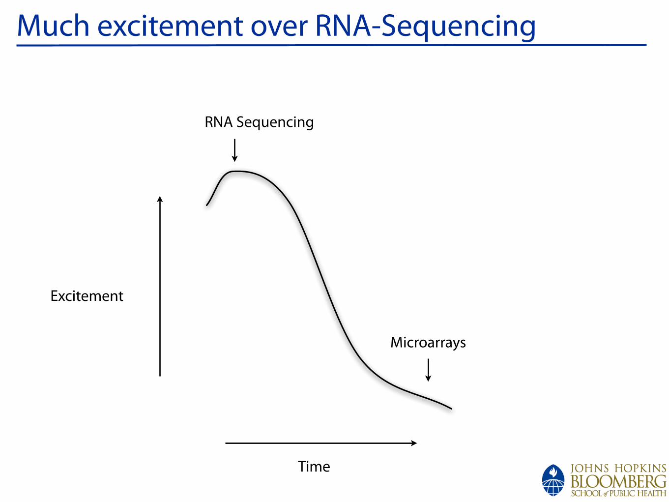
Figure 2 | Reproducibility, linearity and sensitivity. (a) Comparison of two brain technical replicate RNA-Seq determinations for all mouse gene models (from the UCSC genome database), measured in reads per kilobase of exon per million mapped sequence reads (RPKM), which is a normalized measure of exonic read density; R2 = 0.96. (b) Distribution of uniquely mappable reads onto gene parts in the liver sample. Although 93% of the reads fall onto exons or the RNAFAR-enriched regions (see Fig. 3 and text), another 4% of the reads falls onto introns and 3% in intergenic regions. (c) Six in vitro–synthesized reference transcripts of lengths 0.3–10 kb were added to the liver RNA sample (1.2 104 to 1.2 109 transcripts per sample; R2 > 0.99). (d) Robustness of RPKM measurement as a
function of RPKM expression level and depth of sequencing. Subsets of the entire liver dataset (with 41 million mapped unique + splice + multireads) were used to calculate the expression level of genes in four different expression classes to their final expression level. Although the measured expression level of the 211 most highly expressed genes (black and cyan) was effectively unchanged after 8 million mappable reads, the measured expression levels of the other two classes (purple and red) converged more slowly. The fraction of genes for which the measured expression level was within 5% of the final value is reported. 3 RPKM corresponds to approximately one transcript per cell in liver. The corresponding number of spliced reads in each subset is shown on the top x axis.
NATURE METHODS | VOL.5 NO.7 | JULY 2008 | 623
ARTICLES
and phage lambda templates (Fig. 2c). These standards comprised long (~10,000 nt), intermediate (~1,500 nt) and short (~300 nt) transcripts, and they were designed to span the range of abundance (~0.5–50,000 transcripts per cell) typically observed in natural transcriptomes. RNA-Seq data for the standards were linear across a dynamic range of five orders of magnitude in RNA concentra-tion. Sequence coverage over test transcripts was highly reproducible and quite uniform (Supplementary Fig. 1c). At current practical sequencing capacity and cost (~40 M mapped reads), transcript detection was robust at 1.0 RPKM and above for a typical 2-kilo-base (kb) mRNA (~80 individual sequence reads resulting in a P value <10 16). Beyond simple detection confidence, we analyzed the impact of different amounts of sequencing on our ability to measure the concentration of a given transcript class (defined on the basis of RPKM) within ±5% (Fig. 2d). When these RNA standards are used in conjunction with information on cellular RNA content, abso-lute transcript levels per cell can also be calculated. For example, on the basis of literature values for the mRNA content of a liver cell19 and the RNA standards, we estimated that 3 RPKM corresponds to about one transcript per liver cell. For C2C12 tissue culture cells, for
High read number is relevant for RNA-Seq because our ability to reliably detect and measure rare, yet physiologically relevant, RNA species (those with abundances of 1–10 RNAs per cell) depends on the number of independent pieces of evidence (sequence reads) obtained for transcripts from each gene. This constraint influenced our sequencing strategy, choice of instrument and choice of the 25-bp read length.
The sensitivity of RNA-Seq will be a function of both molar con-centration and transcript length. We therefore quantified transcript levels in reads per kilobase of exon model per million mapped reads (RPKM) (Fig. 1a,c). The RPKM measure of read density reflects the molar concentration of a transcript in the starting sample by normalizing for RNA length and for the total read number in the measurement. This facilitates transparent comparison of transcript levels both within and between samples.
Examination of a well-characterized locusData from a 21-million-read transcriptome measurement of adult mouse skeletal muscle (Fig. 1b,c) illustrate some key characteris-tics of our results. Myf6 (also known as Mrf4) is a much-studied myogenic transcription factor gene that is expressed specifically and modestly in mus-cle, as expected, but silent in liver and brain. Evidence for Myf6 expression in skeletal muscle (Fig. 1b) consisted of 1,295 sequence reads 25 bp in length that map uniquely to Myf6 exons, and 30 reads that cross splice junctions; another four reads fell within the introns. Brain and liver measurements of similar total read number had 1 and 0 reads on Myf6 exons, illustrating favorable signal-to-noise characteristics, absolute signal and specificity (Fig. 1c).
RNA-Seq global data propertiesTechnical replicate determinations of transcript abundance were reproducible (R2 = 0.96, Fig. 2a). Summing the replicates over an entire transcriptome (Fig. 2b, liver; Supplementary Table 2 online) showed that the vast majority of reads (93%) mapped to known and predicted exons, even though the exons comprise <2% of the entire genome; 4% of reads were within introns; and only 3% fell in the large intergenic terri-tory. We expected to observe some intronic reads in total poly(A)+ RNA because such preparations are known to include partially processed nuclear RNAs and because some genes might have internal exons that have not yet been added to the gene models. The 3% intergenic fraction places a rough upper bound on possible noise reads.
To assess the dynamic range of RNA-Seq and to test for possible effects of starting transcript length on the observed transcript abundance, we introduced into each exper-imental sample a set of known RNA stan-dards transcribed in vitro from Arabidopsis
Bra
in te
chni
cal 2
(R
PK
M) 104
103
100
10
1
0.0
RP
KM
104
103
100
10
1
0.0
Technical replicatesR2 = 0.96
0.1 1 10 100 1,000 10,000 Brain technical 1 (RPKM)
104 105 106 107 108 109
Reference transcripts per 100 ng mRNA
Sensitivity and dynamic rangeR2 = 0.99
Exons (93%)
Intergenic (3%)
Introns (4%)
1.0
0.8
0.6
0.4
0.2
0
Frac
tion
of g
enes
with
in±5
% o
f fin
al v
alue
0.82
2.
05
4.10
8.
20
16.4
0
24.6
0
32.8
0
41.0
0
0.05
0.
12
0.25
0.
48
0.96
1.44
1.91
2.40
Mapped reads (millions)
Splices (millions)
Robustness of quantification as a function of read number
3,000 + RPKM300–2,999 RPKM30–299 RPKM3–29 RPKM
n = 24n = 187n = 1,591n = 6,369
a b
c d
Figure 2 | Reproducibility, linearity and sensitivity. (a) Comparison of two brain technical replicate RNA-Seq determinations for all mouse gene models (from the UCSC genome database), measured in reads per kilobase of exon per million mapped sequence reads (RPKM), which is a normalized measure of exonic read density; R2 = 0.96. (b) Distribution of uniquely mappable reads onto gene parts in the liver sample. Although 93% of the reads fall onto exons or the RNAFAR-enriched regions (see Fig. 3 and text), another 4% of the reads falls onto introns and 3% in intergenic regions. (c) Six in vitro–synthesized reference transcripts of lengths 0.3–10 kb were added to the liver RNA sample (1.2 104 to 1.2 109 transcripts per sample; R2 > 0.99). (d) Robustness of RPKM measurement as a
function of RPKM expression level and depth of sequencing. Subsets of the entire liver dataset (with 41 million mapped unique + splice + multireads) were used to calculate the expression level of genes in four different expression classes to their final expression level. Although the measured expression level of the 211 most highly expressed genes (black and cyan) was effectively unchanged after 8 million mappable reads, the measured expression levels of the other two classes (purple and red) converged more slowly. The fraction of genes for which the measured expression level was within 5% of the final value is reported. 3 RPKM corresponds to approximately one transcript per cell in liver. The corresponding number of spliced reads in each subset is shown on the top x axis.
NATURE METHODS | VOL.5 NO.7 | JULY 2008 | 623
ARTICLES
(other compelling reasons as well)
Mortazavi (Nat. Methods 2008)
A great paper!

Mapping
!
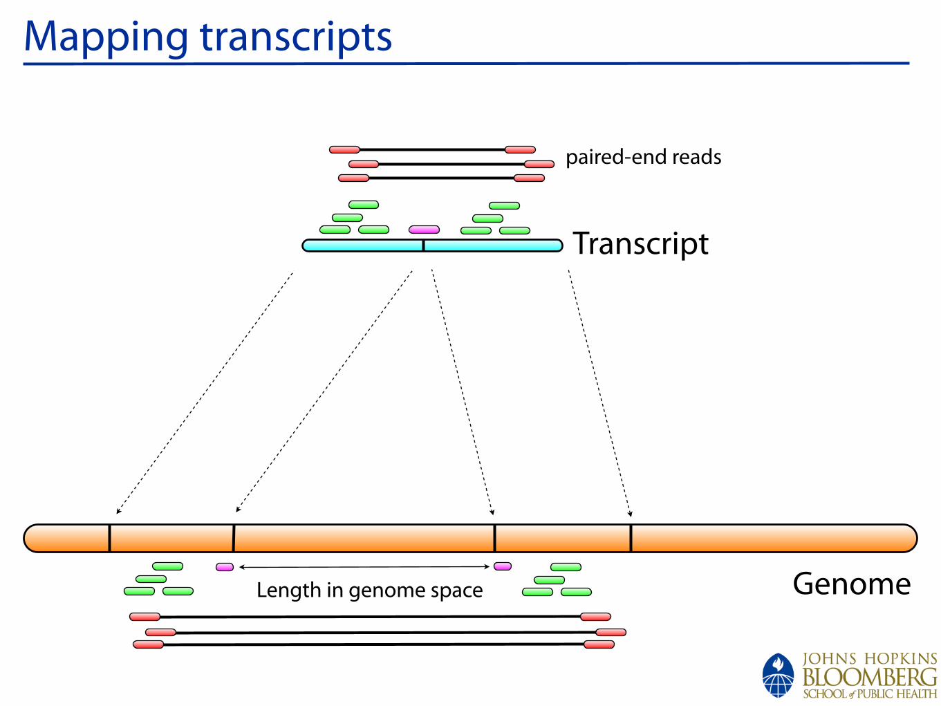
Mapping transcripts
Genome
Transcript
Length in genome space
paired-end reads
!
The basic approachesthe ‘noise’ level generated by mismapped reads or intronic RNA from incompletely spliced heterogenous nuclear RNA (hnRNA). In mouse and human samples, we have especially noticed that prominent read densities often extend well beyond the annotated 3 untranslated regions or as alternatively spliced 5 untranslated regions, internal exons or retained introns. ERANGE, G-Mo.R-Se and TopHat first aggregate reads into transfrags. Whereas G-Mo.R-Se and TopHat rely primarily on spliced reads to connect transfrags together, ERANGE uses two different strategies depending on the availability of paired reads. In the currently conventional unpaired sequence read case, ERANGE assigns transfrags to genes based on an arbitrary user-selected radius, whereas in the paired-end read case, it will bring together transfrags only when they are connected by at least one paired read. Both strategies work much better with data that preserve RNA strandedness.
Quantifying gene expression. Given a gene model and mapped reads, one can sum the read counts for that gene as one measure of the expression level of that gene at that sequencing depth. However, the number of reads from a gene is naturally a function of the length of the mRNA as well as its molar concentration. A simple solution that preserves molarity is to normalize the read count by the length of the mRNA and the number of million mappable reads to obtain reads per kilobase per million (RPKM) values18. RPKMs for genes are then directly comparable within the sample by pro-viding a relative ranking of expression. Although they are straight-forward, RPKM values have several substantive detail differences between software packages, and there are also some caveats in using them. Whereas ERANGE uses a union of known and novel exon models to aggregate reads and determine an RPKM value for the locus, TopHat and RSAT restrict themselves to known or prespeci-fied exons. ERANGE will also include spliced reads and can include assigned multireads in its RPKM calculation, whereas other pack-ages are limited to uniquely mappable reads.
Several experimental issues influence the RPKM quantification, including the integrity of the input RNA, the extent of ribosomal RNA remaining in the sample, size selection steps and the accuracy of the gene models used. RPKMs reflect the true RNA concentration best when samples have relatively uniform sequence coverage across the entire gene model, which is usually approached by using random priming or RNA-ligation protocols, although both protocols cur-rently fall short of providing the desired uniformity. Poly(A) prim-ing has different biases (3 ) from partial extension or when there is partial RNA degradation. Resulting ambiguities in RPKMs from an RNA-seq experiment are akin to microarray intensities that need to be post-processed before comparison to other RNA-seq samples using any number of well-documented normalization methods, such as variance stabilization42, for example.
More sophisticated analyses of RNA-seq data allow users to extract additional information from the data. One area of considerable inter-est and activity is in transcript modeling and quantifying specific isoforms. BASIS calculates transcript levels from coverage of known exons by taking advantage of specifically informative nucleotides from each transcript isoform. A second area is sequence variation. The RNA sequences themselves can be mined to identify positions where the base reported differs from the reference genome(s), identifying either a single-nucleotide polymorphism or a private mutation25,43. When these are heterozygous and phased or informatively related to the source genome, RNA single-nucleotide polymorphisms can be
(SINEs and LINEs) in the untranslated regions of genes as well as the abundance of retroposed pseudogenes for highly expressed housekeeping genes in large genomes. Both of these vary from one genome to the next39. For example, several GAPDH retroposed pseudogenes in the mouse genome differ by less than 2 nucleotides (0.2%) from the mRNA for GAPDH itself, making it difficult to map reads correctly to the originating locus based on RNA-seq data alone. Orthogonal data such as RNA polymerase II occupancy and ChIP-seq measurements can later be brought to bear in some cases, but different software and use parameters make starting choices based on the RNA data alone. Whereas the algorithms are generally sensible, specific cases can be insidious and are worth being aware of. For example, a minority of reads from one paralog can map best to other sites (usually another paralog or pseudogene) because of the error rate in sequencing, which is quite substantial on current platforms (typically around 1%). For highly expressed genes, this can cause a shadow of expression at these pseudogenes, which may then be called as transfrags. Similarly, reads that are intron-spanning from a source gene may map instead perfectly and uniquely to a retroposed pseudogene. The ERANGE package avoids such mis-assignment by mapping reads simultaneously across the genome and splice junctions, thus turning them into multireads that are subsequently handled separately.
Assigning reads to known and new gene models. The next level of RNA-seq analysis associates mapped reads with known or new gene models. Given a set of annotations, all tools can tally the reads that fall on known gene models, and several tools like RSAT40 and BASIS41 deal primarily with the annotated models. However, a sub-stantial fraction of reads fall outside of the annotated exons, above
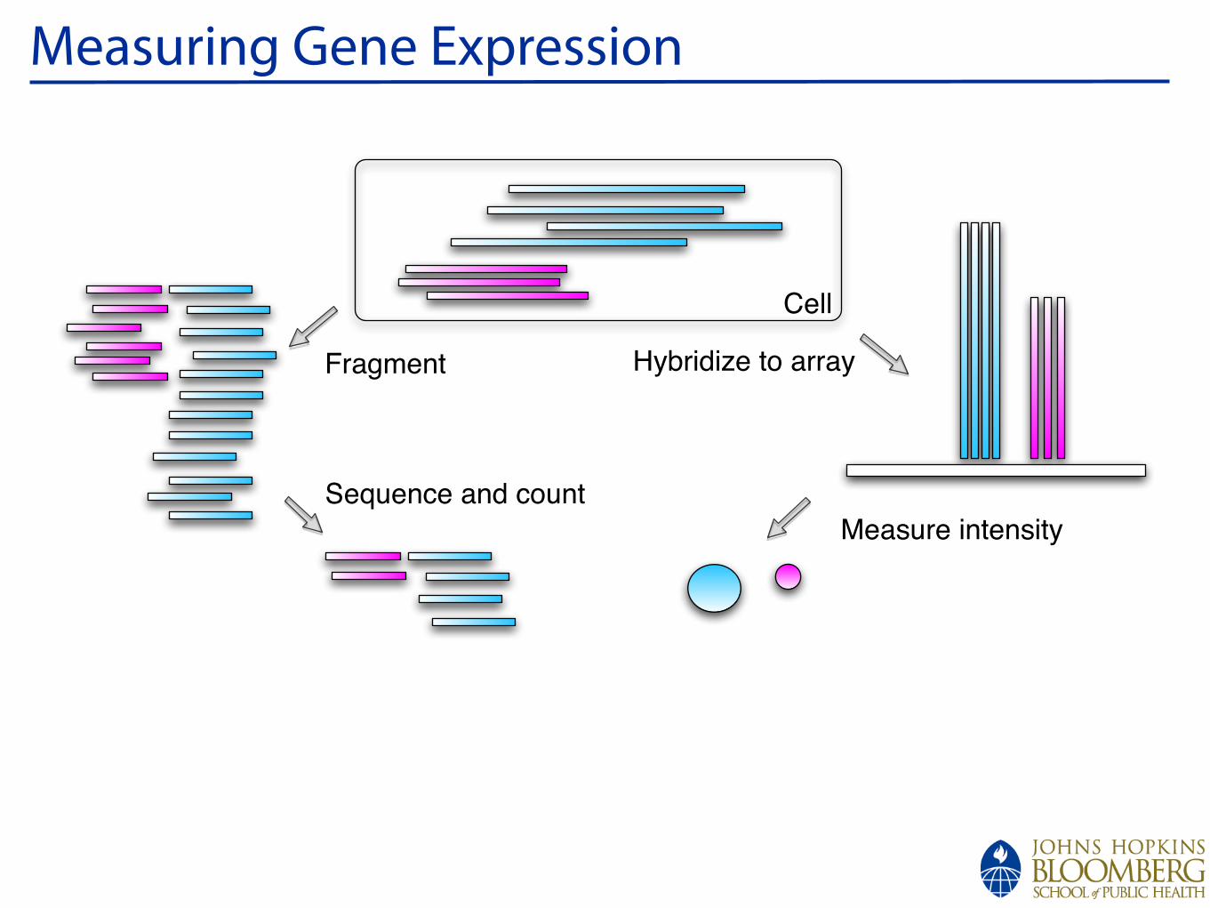
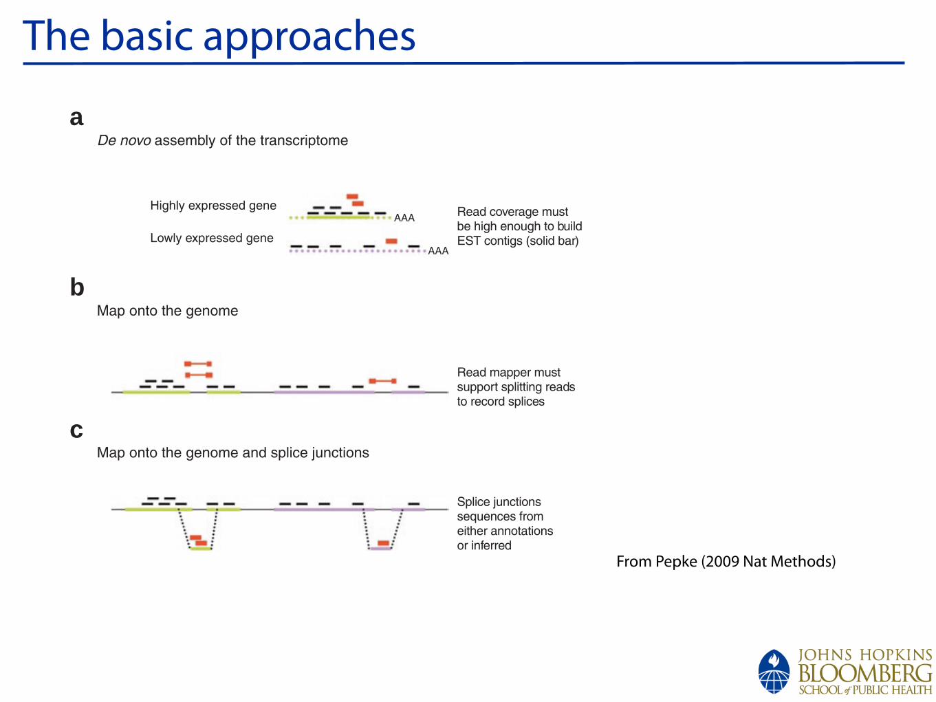
De novo assembly of the transcriptome
Map onto the genome and splice junctions
Map onto the genome
Highly expressed gene
Lowly expressed gene
Read coverage mustbe high enough to buildEST contigs (solid bar)
Read mapper mustsupport splitting readsto record splices
Splice junctionssequences fromeither annotationsor inferred
AAA
AAA
a
b
c
Figure 6 | Approaches to handle spliced reads. (a) In de novo transcriptome assembly, splice-crossing reads (red) will only contribute to a contig (solid green), when the reads are at high enough density to overlap by more than a set of user-defined assembly parameters. Parts of gene models (dotted green) or entire gene models (dotted magenta) can be missed if expressed at sub-threshold. (b) Splice-crossing reads can be mapped directly onto the genome if the reads are long enough to make gapped-read mappers practical. (c) Alternatively, regular short read mappers can be used to map spliced reads ungapped onto supplied additional known or predicted splice junctions.
S30 | VOL.6 NO.11s | NOVEMBER 2009 | NATURE METHODS SUPPLEMENT
REVIEW
From Pepke (2009 Nat Methods)
!
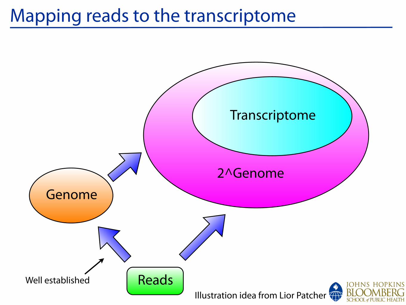
Mapping reads to the transcriptome
Transcriptome
2^Genome
Reads
Genome
Illustration idea from Lior Patcher
Well established
!
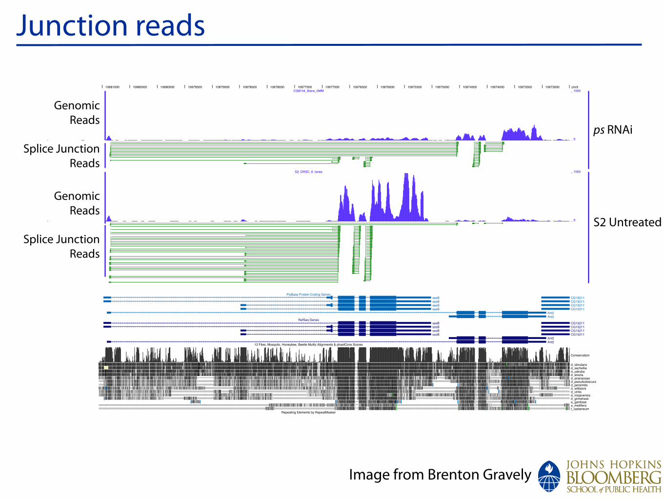
Junction reads
:chrX
Conservation
d_simulansd_sechelliad_yakubad_erectad_ananassaed_pseudoobscurad_persimilisd_willistonid_virilisd_mojavensisd_grimshawia_gambiaea_melliferat_castaneum
1067300010673500106740001067450010675000106755001067600010676500106770001067750010678000106785001067900010679500106800001068050010681000CG8144_6lane_0MM
S2_DRSC_6_lanes
FlyBase Protein-Coding Genes
RefSeq Genes
12 Flies, Mosquito, Honeybee, Beetle Multiz Alignments & phastCons Scores
Repeating Elements by RepeatMasker
CG15211CG15211CG15211CG15211
Ant2Ant2
sesBsesBsesBsesB
CG15211CG15211CG15211CG15211
Ant2Ant2
sesBsesBsesBsesB
_ 1000
_ 0
_ 1000
_ 0
ps RNAi
S2 Untreated
Splice JunctionReads
GenomicReads
Splice JunctionReads
GenomicReads
Image from Brenton Gravely
!
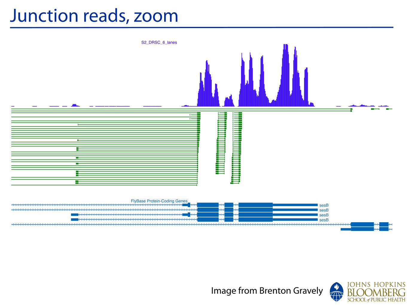
Junction reads, zoom
:chrX
Conservation
d_simulansd_sechelliad_yakubad_erectad_ananassaed_pseudoobscurad_persimilisd_willistonid_virilisd_mojavensisd_grimshawia_gambiaea_melliferat_castaneum
1067300010673500106740001067450010675000106755001067600010676500106770001067750010678000106785001067900010679500106800001068050010681000CG8144_6lane_0MM
S2_DRSC_6_lanes
FlyBase Protein-Coding Genes
RefSeq Genes
12 Flies, Mosquito, Honeybee, Beetle Multiz Alignments & phastCons Scores
Repeating Elements by RepeatMasker
CG15211CG15211CG15211CG15211
Ant2Ant2
sesBsesBsesBsesB
CG15211CG15211CG15211CG15211
Ant2Ant2
sesBsesBsesBsesB
_ 1000
_ 0
_ 1000
_ 0
ps RNAi
S2 Untreated
Splice JunctionReads
GenomicReads
Splice JunctionReads
GenomicReads
Image from Brenton Gravely
!
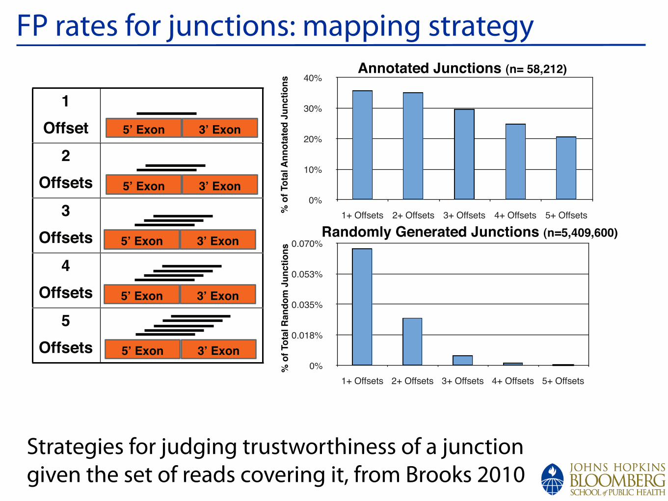
FP rates for junctions: mapping strategy
Strategies for judging trustworthiness of a junction given the set of reads covering it, from Brooks 2010
! "# "! $#
#!###
$# $! %# %!
#
!"#$$%&'$ ()'* +,-./0-/1 2&%&3/45/,6/&7$&8&95,6-:;,3%$&96,3&;,<=>;5-
&'()(*+,*!-*(./)
01)23),45
! "# "! $#
#!###
"!###
$!###
$# $! %# %!
#"####
$####
%####
! "# "! $#
#!###
$# $! %# %!
#
!"#$$%&'$ ()'* +,-./0-/1 2&%&3/45/,6/&7$&8&95,6-:;,3%$&96,3&;,<=>;5-
&'()(*+,*!-*(./)
01)23),45
! "# "! $#
#!###
"!###
$!###
!"#$$%&'$ ()'* +,-./0-/1 2&%&3/45/,6/&7$&8&95,6-:;,3%$&96,3&;,<=>;5-
&'()(*+,*!-*(./)
01)23),45
$# $! %# %!
#"####
$####
%####
% ?@A;,B ?@A;,
Bases on 5’ Exon
32nt 5nt
% ?@A;,B ?@A;,
32nt5nt
At Least 6nt Overhang At Least 6nt Overhang
67
#8
"#8
$#8
%#8
9#8
":*;<<()=( $:*;<<()=( %:*;<<()=( 9:*;<<()=( !:*;<<()=(
#8
#7#">8
#7#%!8
#7#!%8
#7#?#8
":*;<<()=( $:*;<<()=( %:*;<<()=( 9:*;<<()=( !:*;<<()=(
#?
CDD3/-
$?
CDD3/-3
%?
CDD3/-3
2?
CDD3/-3
B?
CDD3/-3 % ?@A;,B ?@A;,
% ?@A;,B ?@A;,
% ?@A;,B ?@A;,
% ?@A;,B ?@A;,
% ?@A;,B ?@A;,
8,,;-0-/1?E5,6-:;,3?F,G?B"H$#$I
)0,1;J<=?K/,/.0-/1?E5,6-:;,3?F,GBH2!LHM!!I
N?;D?O;-0<?8,,;-0-/1?E5,6-:;,3
N?;D?O;-0<?)0,1;J?E5,6-:;,3
&7
Supplemental Figure 3. Analysis of optimal overhang and mismatch for splice junction alignments. (A) Distribution of Overhang Positions ! 5nt. A histogram of the number of uniquely aligned reads across all annotated junctions is shown. An even distribution of read alignments across all base positions occurs if at least a 6nt overhang is enforced. (B) Distinguishing true junctions from false positive alignments. To reduce the number of false positive junctions, as determined by randomly generated junctions, a total of 3 alignment start positions (offsets) were required to consider a junction to be truly present.
Brooks et al. Supplemental
15
!
Mapping - conclusionsMapping to transcript space is not easy.
But essential for really understanding alternative splicing.
Brooks, A.N. et al. Conservation of an RNA regulatory map between Drosophila and mammals. Genome Res 21, 193-202 (2011).
Trapnell, C. et al. Transcript assembly and quantification by RNA-Seq reveals unannotated transcripts and isoform switching during cell differentiation. Nat Biotechnol 28, 511-515 (2010).
Trapnell, C., Pachter, L. & Salzberg, S.L. TopHat: discovering splice junctions with RNA-Seq. Bioinformatics 25, 1105-1111 (2009).
Bias
!
Data from D. melanogaster:chrX
Conservation
d_simulansd_sechelliad_yakubad_erectad_ananassaed_pseudoobscurad_persimilisd_willistonid_virilisd_mojavensisd_grimshawia_gambiaea_melliferat_castaneum
1067300010673500106740001067450010675000106755001067600010676500106770001067750010678000106785001067900010679500106800001068050010681000CG8144_6lane_0MM
S2_DRSC_6_lanes
FlyBase Protein-Coding Genes
RefSeq Genes
12 Flies, Mosquito, Honeybee, Beetle Multiz Alignments & phastCons Scores
Repeating Elements by RepeatMasker
CG15211CG15211CG15211CG15211
Ant2Ant2
sesBsesBsesBsesB
CG15211CG15211CG15211CG15211
Ant2Ant2
sesBsesBsesBsesB
_ 1000
_ 0
_ 1000
_ 0
ps RNAi
S2 Untreated
Splice JunctionReads
GenomicReads
Splice JunctionReads
GenomicReads
Image from Brenton Gravely
!
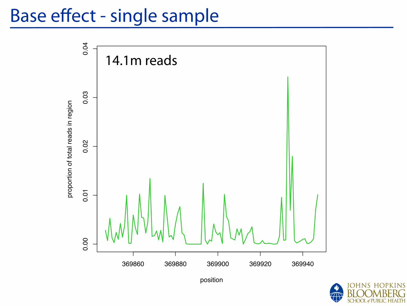
Base effect - single sample
14.1m reads
369860 369880 369900 369920 369940
0.0
00.0
10.0
20.0
30.0
4
gene: YLR110C
position
pro
port
ion o
f to
tal re
ads in r
egio
n
!
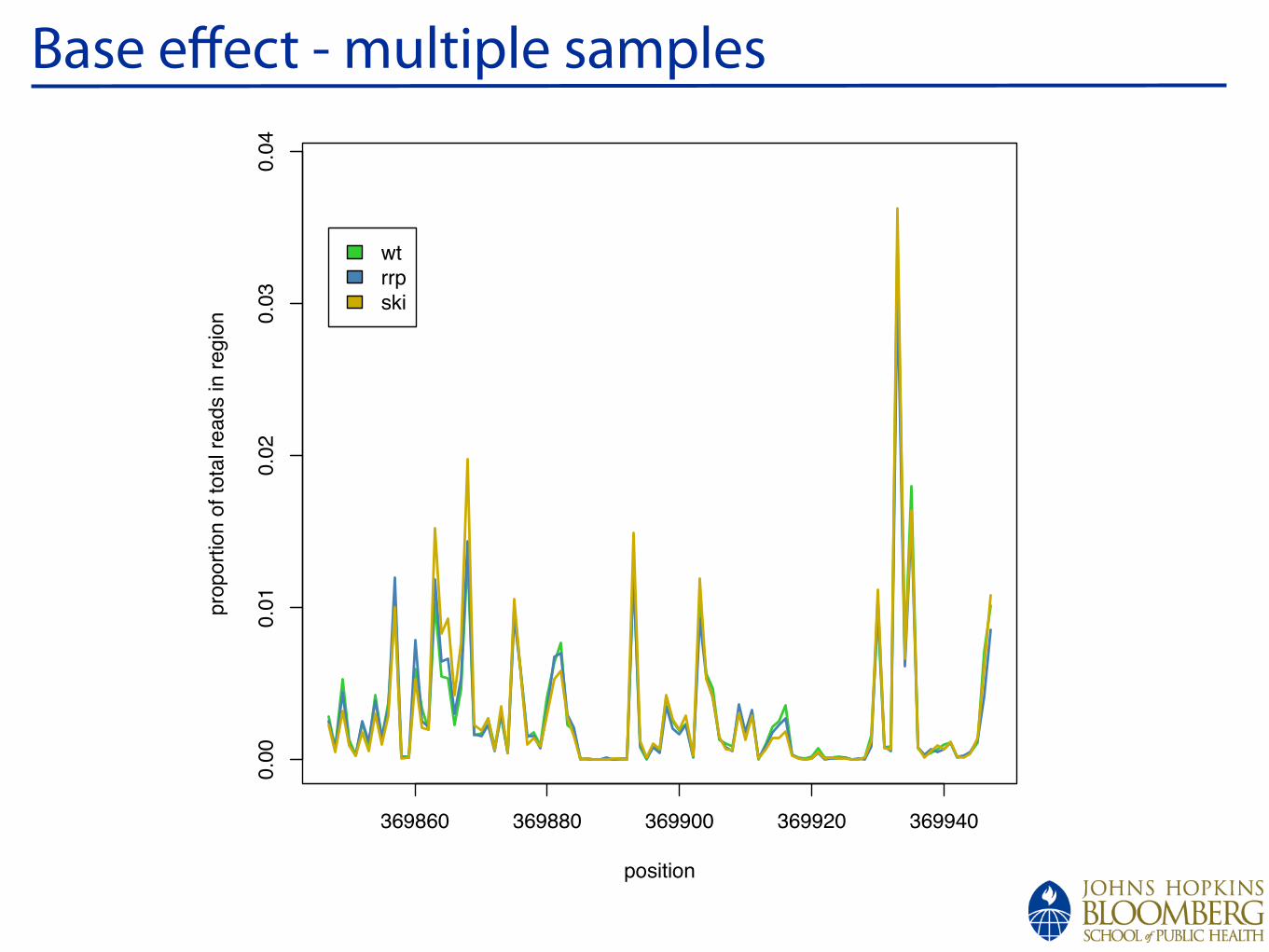
Base effect - multiple samples
369860 369880 369900 369920 369940
0.0
00.0
10.0
20.0
30.0
4
gene: YLR110C
position
pro
port
ion o
f to
tal re
ads in r
egio
n
wt
rrp
ski
!
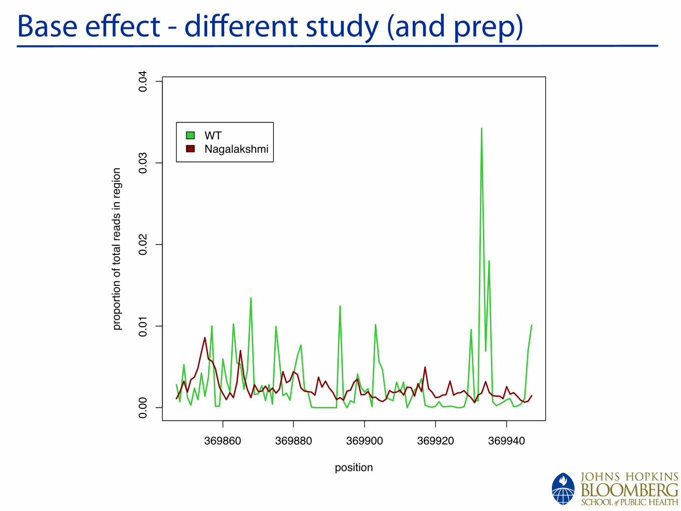
Base effect - different study (and prep)
369860 369880 369900 369920 369940
0.0
00.0
10.0
20.0
30.0
4
gene: YLR110C
position
pro
port
ion o
f to
tal re
ads in r
egio
n
WT
Nagalakshmi
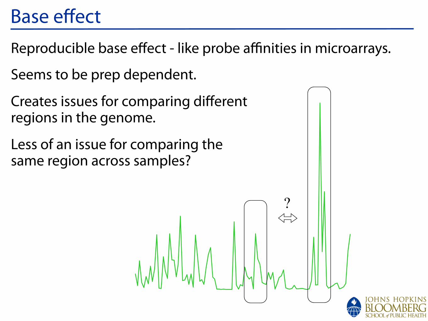
!
Base effectReproducible base effect - like probe affinities in microarrays.
Seems to be prep dependent.
Creates issues for comparing differentregions in the genome.
Less of an issue for comparing thesame region across samples?
369860 369880 369900 369920 369940
0.0
00.0
10.0
20.0
30.0
4
gene: YLR110C
position
pro
port
ion o
f to
tal re
ads in r
egio
n
?
!
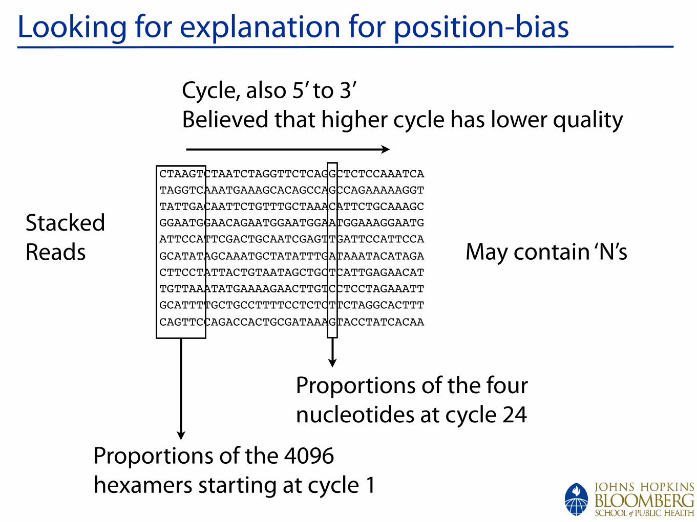
Looking for explanation for position-bias
CTAAGTCTAATCTAGGTTCTCAGGCTCTCCAAATCATAGGTCAAATGAAAGCACAGCCAGCCAGAAAAAGGTTATTGACAATTCTGTTTGCTAAACATTCTGCAAAGCGGAATGGAACAGAATGGAATGGAATGGAAAGGAATGATTCCATTCGACTGCAATCGAGTTGATTCCATTCCAGCATATAGCAAATGCTATATTTGATAAATACATAGACTTCCTATTACTGTAATAGCTGCTCATTGAGAACATTGTTAAATATGAAAAGAACTTGTCCTCCTAGAAATTGCATTTTGCTGCCTTTTCCTCTCTTCTAGGCACTTTCAGTTCCAGACCACTGCGATAAAGTACCTATCACAA
Cycle, also 5’ to 3’Believed that higher cycle has lower quality
StackedReads
Proportions of the four nucleotides at cycle 24
Proportions of the 4096hexamers starting at cycle 1
May contain ‘N’s
!
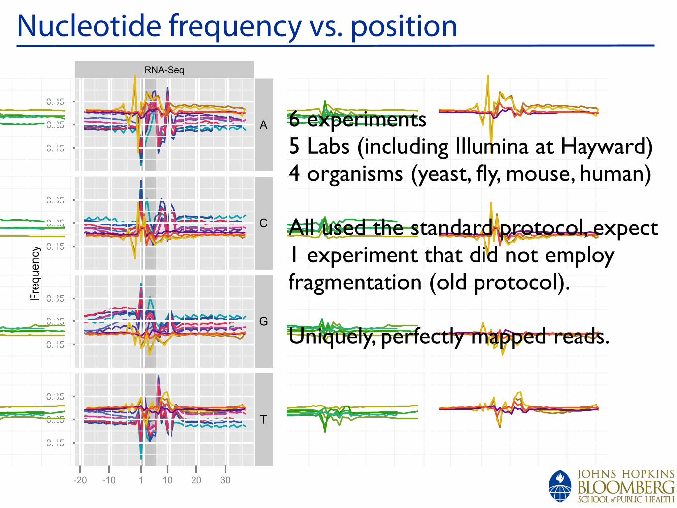
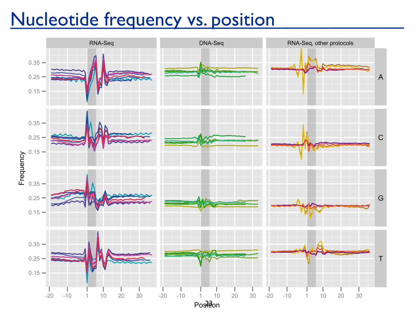
Nucleotide frequency vs. position
Biases in Illumina RNA-Seq, Supplementary Material 7
Supplementary Figures
Position
Frequency
0.15
0.25
0.35
0.15
0.25
0.35
0.15
0.25
0.35
0.15
0.25
0.35
RNA-Seq
-20 -10 1 10 20 30
DNA-Seq
-20 -10 1 10 20 30
RNA-Seq, other protocols
-20 -10 1 10 20 30
A
C
G
T
!"##$%&
'$%()*(
')%+$,$-(
.//
0$*1234%$(*
0$*1235/$%+
!/*+#/6
0$*123789
:5($*1
'(;;/#</*
'/(<<*/%
=5(3>
8$1$#$;5<?(23@A
8$1$#$;5<?(237B
C%$-/#/6
0(#5/#?
!#))?
@893D%$1?/*+$+()*2
@$*E35/FE3=%(?(*1
8)3D%$1?/*+$+()*2
@$*E35/FE3=%(?(*1
789GH/I :5JKGH/I L#(1)G&B3=%(?(*12
8/4"#(,$+()*3M789N
L#(1)G&B3=%(?(*12
78$</3J3M789N
@(4)G?(*"<
L#(1)G&B3=%(?(*12
H)*(O$+()*3M789N
@$*E35/FE3=%(?(*12
78$</3J3M789N
Supplementary Figure S1. Nucleotide frequency vs. position for stringently mapped reads. For each experiment,mapped reads were extended upstream of the 5’ start position, such that the first position of the actual read is 1and positions 0 to -10 are obtained from the mapping to the genome. The first hexamer of the read is shaded darkgrey. The experiments under “RNA-Seq” were all conducted using random hexamer priming, in most casespreceded by fragmentation of the RNA (two experiments did not use fragmentation). The “DNA-Seq”experiments were done using the standard DNA sequencing protocol and consist of a variety of resequencing andChIP-Seq experiments. The “RNA-Seq, other protocols” experiments were conducted using a variety ofprotocols: oligo-dT priming followed by fragmentation using nebulization, sonication, and DNase I, as well asrandom hexamer priming followed by DNase fragmentation, see also Supplementary Table S4.
6 experiments5 Labs (including Illumina at Hayward)4 organisms (yeast, fly, mouse, human)
All used the standard protocol, expect 1 experiment that did not employ fragmentation (old protocol).
Uniquely, perfectly mapped reads.
Biases in Illumina RNA-Seq, Supplementary Material 7
Supplementary Figures
Position
Frequency
0.15
0.25
0.35
0.15
0.25
0.35
0.15
0.25
0.35
0.15
0.25
0.35
RNA-Seq
-20 -10 1 10 20 30
DNA-Seq
-20 -10 1 10 20 30
RNA-Seq, other protocols
-20 -10 1 10 20 30
A
C
G
T
!"##$%&
'$%()*(
')%+$,$-(
.//
0$*1234%$(*
0$*1235/$%+
!/*+#/6
0$*123789
:5($*1
'(;;/#</*
'/(<<*/%
=5(3>
8$1$#$;5<?(23@A
8$1$#$;5<?(237B
C%$-/#/6
0(#5/#?
!#))?
@893D%$1?/*+$+()*2
@$*E35/FE3=%(?(*1
8)3D%$1?/*+$+()*2
@$*E35/FE3=%(?(*1
789GH/I :5JKGH/I L#(1)G&B3=%(?(*12
8/4"#(,$+()*3M789N
L#(1)G&B3=%(?(*12
78$</3J3M789N
@(4)G?(*"<
L#(1)G&B3=%(?(*12
H)*(O$+()*3M789N
@$*E35/FE3=%(?(*12
78$</3J3M789N
Supplementary Figure S1. Nucleotide frequency vs. position for stringently mapped reads. For each experiment,mapped reads were extended upstream of the 5’ start position, such that the first position of the actual read is 1and positions 0 to -10 are obtained from the mapping to the genome. The first hexamer of the read is shaded darkgrey. The experiments under “RNA-Seq” were all conducted using random hexamer priming, in most casespreceded by fragmentation of the RNA (two experiments did not use fragmentation). The “DNA-Seq”experiments were done using the standard DNA sequencing protocol and consist of a variety of resequencing andChIP-Seq experiments. The “RNA-Seq, other protocols” experiments were conducted using a variety ofprotocols: oligo-dT priming followed by fragmentation using nebulization, sonication, and DNase I, as well asrandom hexamer priming followed by DNase fragmentation, see also Supplementary Table S4.
Nucleotide frequency vs. position
Biases in Illumina RNA-Seq, Supplementary Material 7
Supplementary Figures
Position
Frequency
0.15
0.25
0.35
0.15
0.25
0.35
0.15
0.25
0.35
0.15
0.25
0.35
RNA-Seq
-20 -10 1 10 20 30
DNA-Seq
-20 -10 1 10 20 30
RNA-Seq, other protocols
-20 -10 1 10 20 30
A
C
G
T
!"##$%&
'$%()*(
')%+$,$-(
.//
0$*1234%$(*
0$*1235/$%+
!/*+#/6
0$*123789
:5($*1
'(;;/#</*
'/(<<*/%
=5(3>
8$1$#$;5<?(23@A
8$1$#$;5<?(237B
C%$-/#/6
0(#5/#?
!#))?
@893D%$1?/*+$+()*2
@$*E35/FE3=%(?(*1
8)3D%$1?/*+$+()*2
@$*E35/FE3=%(?(*1
789GH/I :5JKGH/I L#(1)G&B3=%(?(*12
8/4"#(,$+()*3M789N
L#(1)G&B3=%(?(*12
78$</3J3M789N
@(4)G?(*"<
L#(1)G&B3=%(?(*12
H)*(O$+()*3M789N
@$*E35/FE3=%(?(*12
78$</3J3M789N
Supplementary Figure S1. Nucleotide frequency vs. position for stringently mapped reads. For each experiment,mapped reads were extended upstream of the 5’ start position, such that the first position of the actual read is 1and positions 0 to -10 are obtained from the mapping to the genome. The first hexamer of the read is shaded darkgrey. The experiments under “RNA-Seq” were all conducted using random hexamer priming, in most casespreceded by fragmentation of the RNA (two experiments did not use fragmentation). The “DNA-Seq”experiments were done using the standard DNA sequencing protocol and consist of a variety of resequencing andChIP-Seq experiments. The “RNA-Seq, other protocols” experiments were conducted using a variety ofprotocols: oligo-dT priming followed by fragmentation using nebulization, sonication, and DNase I, as well asrandom hexamer priming followed by DNase fragmentation, see also Supplementary Table S4.
23
!
Bias - conclusionsThere is clear bias in RNA-Seq
But how much, why and how to deal with it are still open problems.
Hansen, K.D., Brenner, S.E. & Dudoit, S. Biases in Illumina transcriptome sequencing caused by random hexamer priming. Nucleic Acids Res 38, e131 (2010).
Li, J., Jiang, H. & Wong, W.H. Modeling non-uniformity in short-read rates in RNA-Seq data. Genome Biol 11, R50-R50 (2010).
Roberts, A., Trapnell, C., Donaghey, J., Rinn, J.L. & Pachter, L. Improving RNA-Seq expression estimates by correcting for fragment bias. Genome Biol 12, R22 (2011).

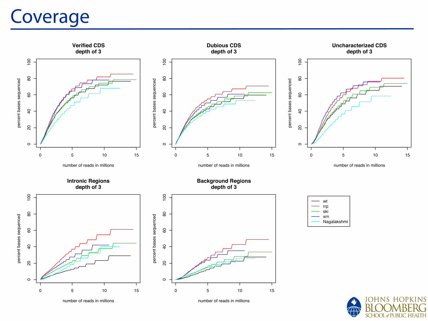
Coverage
!
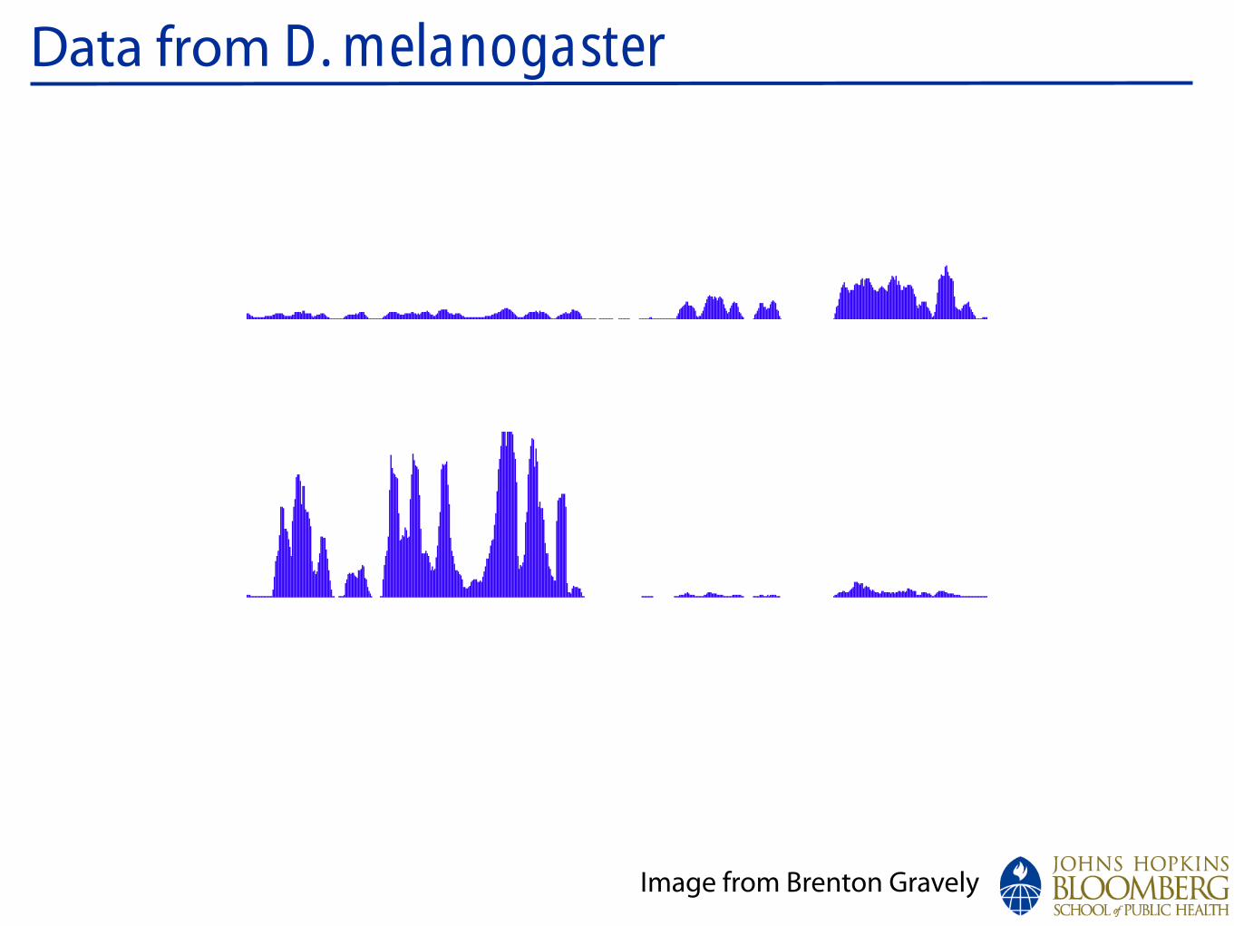
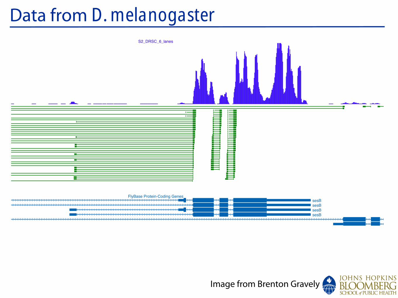
Data from D. melanogaster
:chrX
Conservation
d_simulansd_sechelliad_yakubad_erectad_ananassaed_pseudoobscurad_persimilisd_willistonid_virilisd_mojavensisd_grimshawia_gambiaea_melliferat_castaneum
1067300010673500106740001067450010675000106755001067600010676500106770001067750010678000106785001067900010679500106800001068050010681000CG8144_6lane_0MM
S2_DRSC_6_lanes
FlyBase Protein-Coding Genes
RefSeq Genes
12 Flies, Mosquito, Honeybee, Beetle Multiz Alignments & phastCons Scores
Repeating Elements by RepeatMasker
CG15211CG15211CG15211CG15211
Ant2Ant2
sesBsesBsesBsesB
CG15211CG15211CG15211CG15211
Ant2Ant2
sesBsesBsesBsesB
_ 1000
_ 0
_ 1000
_ 0
ps RNAi
S2 Untreated
Splice JunctionReads
GenomicReads
Splice JunctionReads
GenomicReads
Image from Brenton Gravely
!
0 5 10 15
020
40
60
80
100
Verified CDSdepth of 3
number of reads in millions
perc
ent bases s
equenced
0 5 10 15
020
40
60
80
100
Dubious CDSdepth of 3
number of reads in millions
perc
ent bases s
equenced
0 5 10 15
020
40
60
80
100
Uncharacterized CDSdepth of 3
number of reads in millions
perc
ent bases s
equenced
0 5 10 15
020
40
60
80
100
Intronic Regionsdepth of 3
number of reads in millions
perc
ent bases s
equenced
0 5 10 15
020
40
60
80
100
Background Regionsdepth of 3
number of reads in millions
perc
ent bases s
equenced
wt
rrp
ski
xrn
Nagalakshmi
Coverage
!
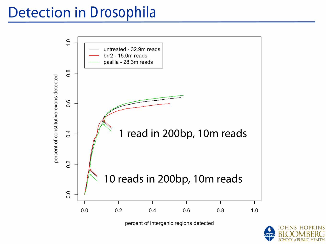
Detection in Drosophila
0.0 0.2 0.4 0.6 0.8 1.0
0.0
0.2
0.4
0.6
0.8
1.0
percent of intergenic regions detected
perc
ent of constitu
tive e
xons d
ete
cte
duntreated - 32.9m reads
brr2 - 15.0m reads
pasilla - 28.3m reads
1 read in 200bp, 10m reads
10 reads in 200bp, 10m reads
Differential Expression
!
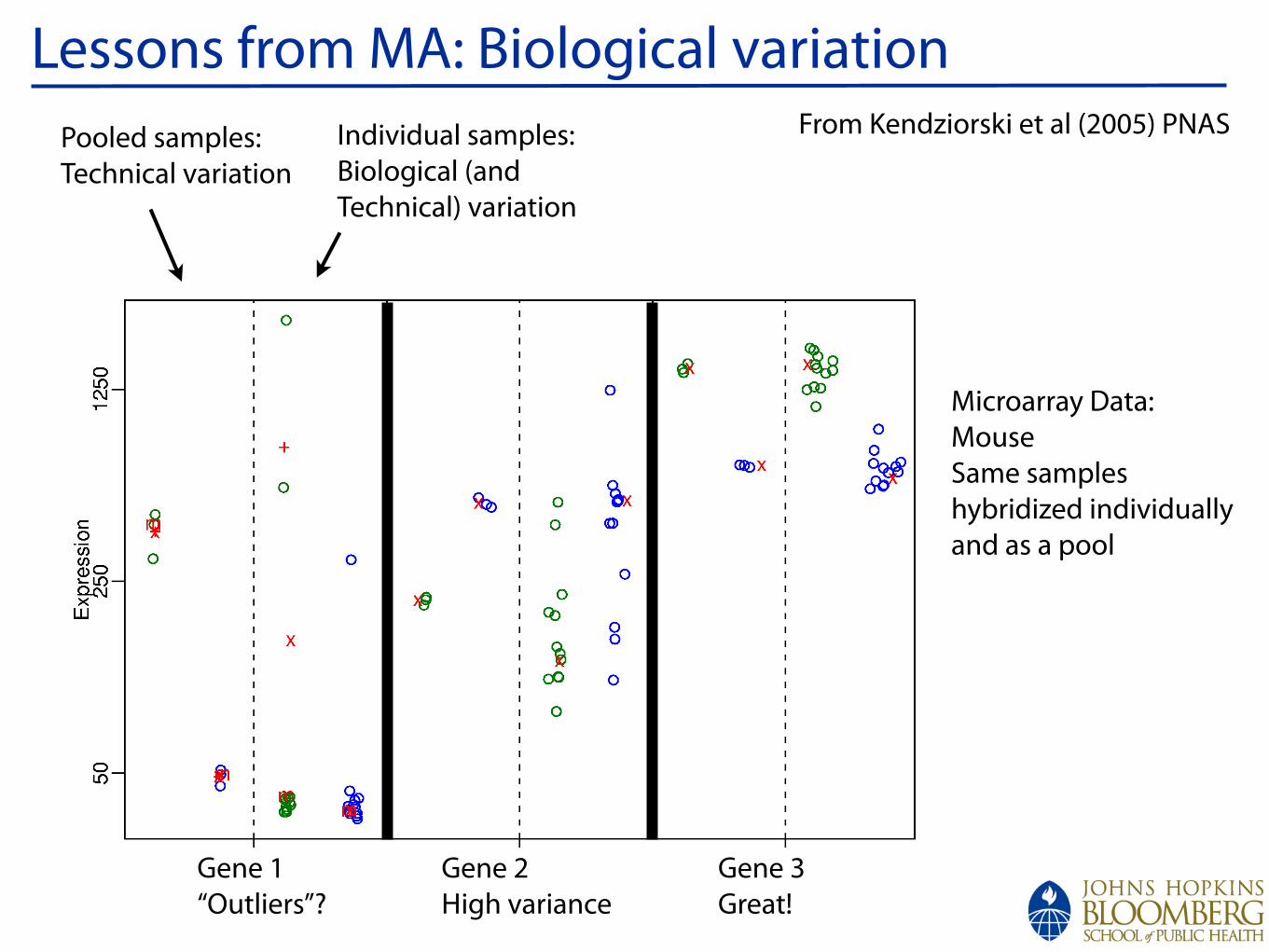
Lessons from MA: Biological variationIndividual samples:Biological (and Technical) variation
Pooled samples:Technical variation
Gene 1“Outliers”?
Gene 2High variance
Gene 3Great!
Microarray Data:MouseSame sampleshybridized individually and as a pool
From Kendziorski et al (2005) PNAS
!
What is our measure of “gene expression”?
With microarrays, we have prede#ned features which collect measurements for a given gene.
Here we need to ask:
• What is a gene?
• What is the expression level of the gene, given our observed data?
!
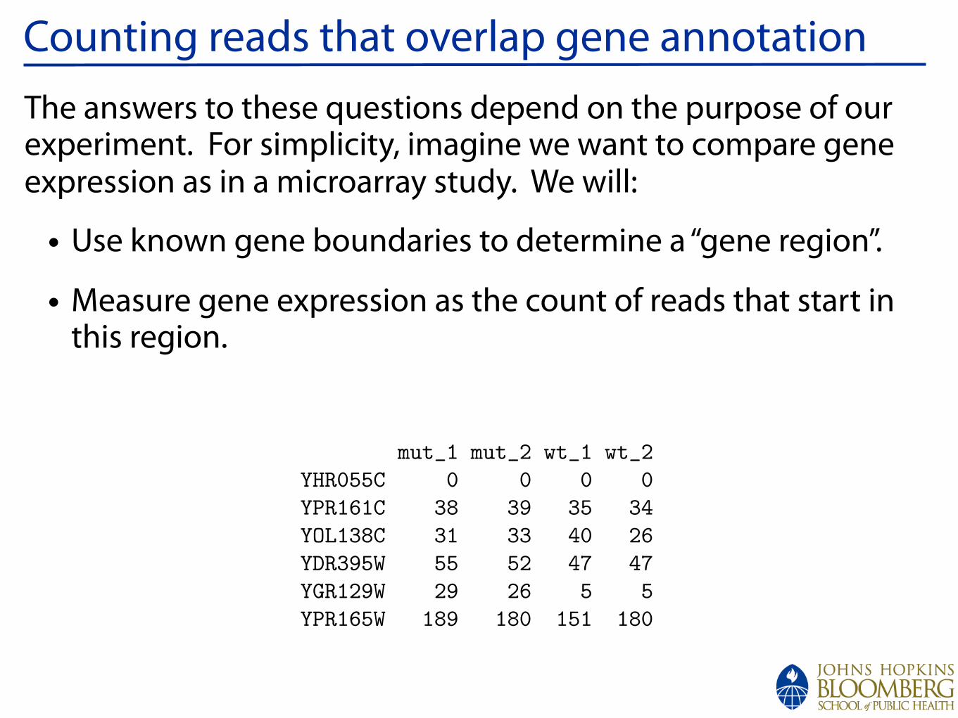
Counting reads that overlap gene annotationThe answers to these questions depend on the purpose of our experiment. For simplicity, imagine we want to compare gene expression as in a microarray study. We will:
• Use known gene boundaries to determine a “gene region”.
• Measure gene expression as the count of reads that start in this region.
Associating Annotation to Reads
At an abstract level, we want to apply a function that associates thealigned read data to the relevant regions of annotation and then countsthe number of reads that fall into each gene. This will be our measure ofgene expression.
First, we need to determine in which range each read lands. At the endof the day, we want a data structure that looks more or less like this:
> head(geneLevelData)
mut_1 mut_2 wt_1 wt_2YHR055C 0 0 0 0YPR161C 38 39 35 34YOL138C 31 33 40 26YDR395W 55 52 47 47YGR129W 29 26 5 5YPR165W 189 180 151 180
16 / 1
!
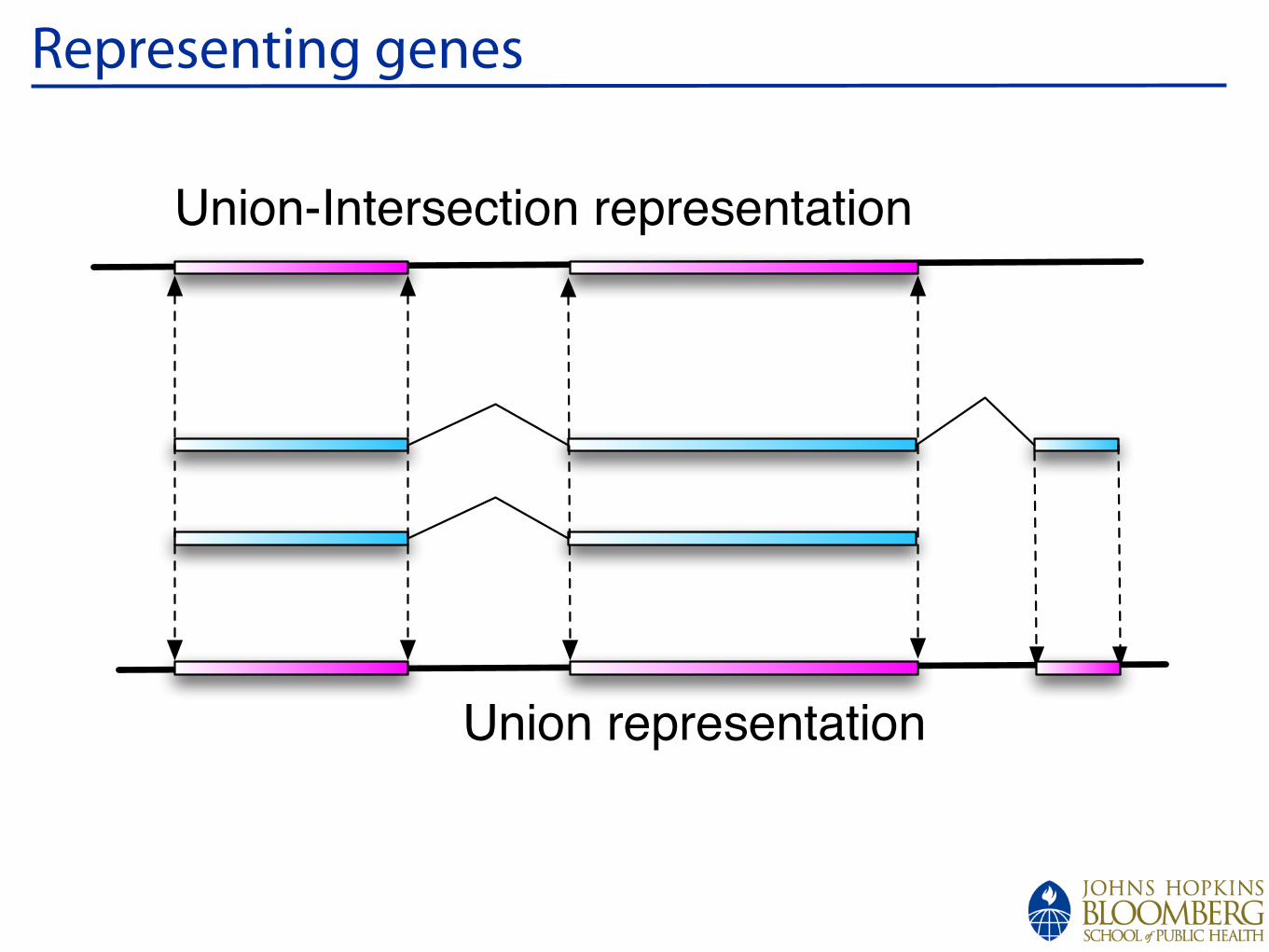
Representing genes
Union-Intersection representation
Union representation
!
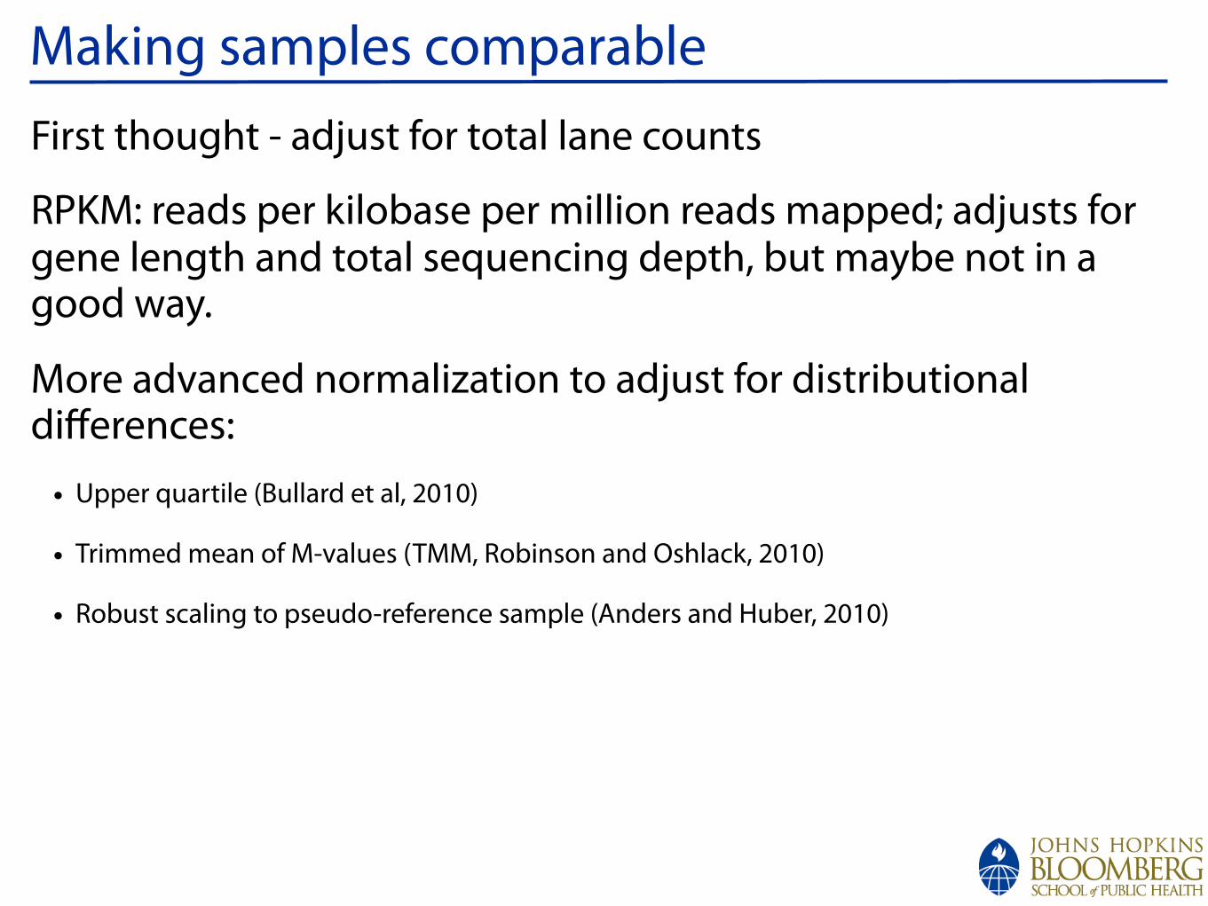
Making samples comparableFirst thought - adjust for total lane counts
RPKM: reads per kilobase per million reads mapped; adjusts for gene length and total sequencing depth, but maybe not in a good way.
More advanced normalization to adjust for distributional differences:
• Upper quartile (Bullard et al, 2010)
• Trimmed mean of M-values (TMM, Robinson and Oshlack, 2010)
• Robust scaling to pseudo-reference sample (Anders and Huber, 2010)
!
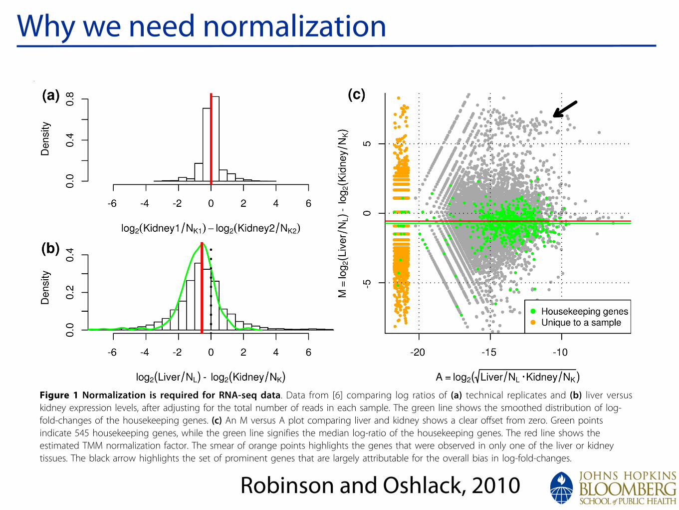
Why we need normalization
Other datasetsThe global shift in log-fold-change caused by RNA com-position differences occurs at varying degrees in otherRNA-seq datasets. For example, an M versus A plot forthe Cloonan et al. [12] dataset (Figure S3 in Additionalfile 1) gives an estimated TMM scaling factor of 1.04between the two samples (embryoid bodies versusembryonic stem cells), sequenced on the SOLiD™ sys-tem. The M versus A plot for this dataset also highlightsan interesting set of genes that have lower overall
expression, but higher in embryoid bodies. This explainsthe positive shift in log-fold-changes for the remaininggenes. The TMM scale factor appears close to the med-ian log-fold-changes amongst a set of approximately 500mouse housekeeping genes (from [17]). As anotherexample, the Li et al. [18] dataset, using the llumina 1GGenome Analyzer, exhibits a shift in the overall distri-bution of log-fold-changes and gives a TMM scaling fac-tor of 0.904 (Figure S4 in Additional file 1). However,there are sequencing-based datasets that have quitesimilar RNA outputs and may not need a significantadjustment. For example, the small-RNA-seq data fromKuchenbauer et al. [19] exhibits only a modest bias inthe log-fold-changes (Figure S5 in Additional file 1).Spike-in controls have the potential to be used for
normalization. In this scenario, small but knownamounts of RNA from a foreign organism are added toeach sample at a specified concentration. In order touse spike-in controls for normalization, the ratio of theconcentration of the spike to the sample must be keptconstant throughout the experiment. In practice, this isdifficult to achieve and small variations will lead tobiased estimation of the normalization factor. For exam-ple, using the spiked-in DNA from the Mortazavi et al.data set [11] would lead to unrealistic normalization fac-tor estimates (Figure S6 in Additional file 1). As with
Figure 1 Normalization is required for RNA-seq data. Data from [6] comparing log ratios of (a) technical replicates and (b) liver versuskidney expression levels, after adjusting for the total number of reads in each sample. The green line shows the smoothed distribution of log-fold-changes of the housekeeping genes. (c) An M versus A plot comparing liver and kidney shows a clear offset from zero. Green pointsindicate 545 housekeeping genes, while the green line signifies the median log-ratio of the housekeeping genes. The red line shows theestimated TMM normalization factor. The smear of orange points highlights the genes that were observed in only one of the liver or kidneytissues. The black arrow highlights the set of prominent genes that are largely attributable for the overall bias in log-fold-changes.
Table 1 Number of genes called differentially expressedbetween liver and kidney at a false discovery rate <0.001using different normalization methods
Library sizenormalization
TMMnormalization
Overlap
Higher in liver 2,355 4,293 2,355
Higher inkidney
8,332 4,935 4,935
Total 10,867 9,228 7,290
House keepinggenes (545)
Higher in liver 45 137 45
Higher inkidney
376 220 220
Total 421 357 265
TMM, trimmed mean of M values.
Robinson and Oshlack Genome Biology 2010, 11:R25http://genomebiology.com/2010/11/3/R25
Page 4 of 9
Robinson and Oshlack, 2010
!
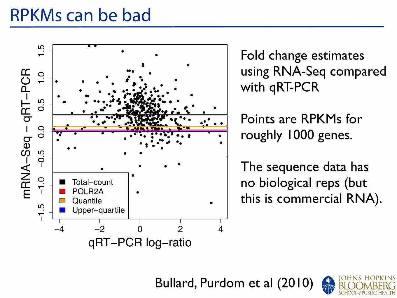
RPKMs can be bad
!
!
!
!
!
!
!
!
!
!
!
!
!
!
!
!!
!!
!!
!
!
!
!
!
!
!
!
!
!
!
!
!
!!
!
!
!
!
!
!
!
!
!
!
!
!
!
!
!
!
!
!
!
!
!
!
!
!
!
!
!
!
!
!!
!
!
!
!
!
!!!
!
!
!
!
!
!
!
!
!!
!
!
!
!
!
!
!
!
!
!
!
!
!
!
!
!!
!
!
!
!
!
!!
!
!
!
!
!!
!
!
!
!
!
!
!!
!
!
!
!!
!
!
!
!
!
!
!
!
!
!!
!
!!!
!
!
!
!
!
!
!
!
!
!
!
!
!
!
!!
!
!!
!
!
!
!
!!
!
!
!!
!
!
!
!
!
!
!
!
!
!
!
!
!
!
!
!!
!
!
!!!
!
!
!
!
!
!
!
!
!
!!
!
!
!
!
!
!
!
!
!
!
!
!
!
!
!!
!!
!
!!
!
!
!
!
!
!
!
!
!!!
!
!
!
!
!
!
!
!
!
!
!
!
!
!
!!
!
!
!
!
!
!
!
!
!
!
!
!
!
!
!
!
!
!
!
!
!
!
!!
!
!
!
!
!
!
!!
!
!!
!
!
!
!
!!
!!
!
!
!
!!
!
!
!
!
!
!
!
!!
!
!
!
!
!
!
!!
!
!
!
!
!!
!
!
!
!
!
!
!
!
!
!!
!!
!!!!
!
!
!
!
!
!
!
!
!!
!
!
!
!
!
!
!
!!
!
!!
!
!
!
!
!
!
!
!
!
!
!
!
!
!
!
!!
!
!
!
!!
!
!
!
!
!
!
!
!
!
!
!
!
!
!
!
!
!
!
!
!
!
!
!
!
!
!
!!
!!
!
!
!
!!
!
!
!
!
!
!
!
!
!
!
!
!
!
!!
!
!
!
!
!
!
!
!
!
!
!!
!
!
!
!
!
!!
!
!
!
!!
!
!
!
!
!
!
!
!
!
!
!!
!
!
−4 −2 0 2 4
−1.5
−1.0
−0.5
0.0
0.5
1.0
1.5
qRT−PCR log−ratio
mRN
A−Se
q −
qRT−
PCR
Total−countPOLR2AQuantileUpper−quartile
Fold change estimates using RNA-Seq compared with qRT-PCR
Points are RPKMs forroughly 1000 genes.
The sequence data has no biological reps (but this is commercial RNA).
Bullard, Purdom et al (2010)
!
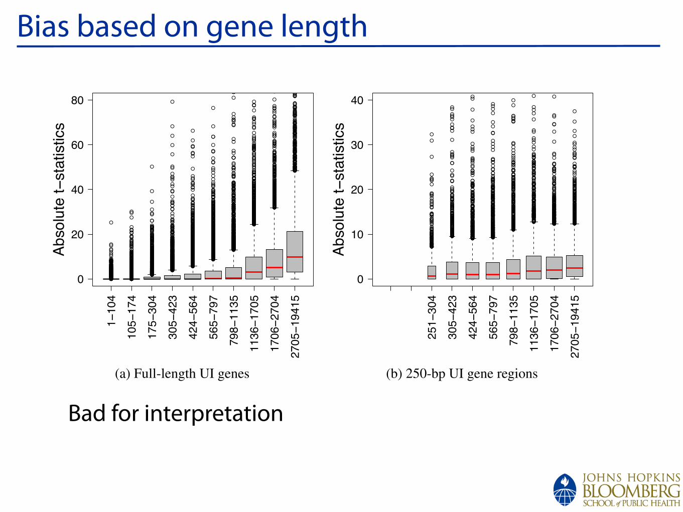
Bias based on gene length
!!!!!!
!
!!
!
!
!
!
!!!
!
!
!
!!
!
!!!!
!!!
!
!
!!!!!!!
!
!
!
!
!
!!!!
!
!!!
!
!
!
!!!!!!
!
!!!!
!
!!!!!
!
!!!!!
!
!!
!
!
!
!
!
!!!!
!!!!!
!!
!
!!!
!!!
!
!
!!!
!!!!
!
!
!!!!!
!
!
!
!!!!
!
!
!!
!
!!
!
!
!!!!!
!!!!!!!!!!!
!
!!!!
!!!!
!
!!!!
!
!!!
!!!!!!
!!!!
!
!
!!!!!
!
!
!!
!!
!
!!
!
!
!!!!!!!
!!!!!!!!!!!
!!!
!
!
!!!!!!!
!!
!
!!!!!!
!!!!!!
!
!
!
!!!!!!!!!
!
!
!
!
!
!!
!
!!!
!
!!
!
!!!!!!
!
!
!!
!!!!!
!
!
!!!
!
!
!
!!!!!!!!!!!!!
!!!
!
!
!
!!!!!
!!!!
!!!
!!!!
!
!!!!!
!!!
!!
!
!!
!
!!!
!!!!!!!!
!!!
!!!!!!!!!!!!!!!
!
!!!!
!!
!
!!!!!!!!!!
!!!!!
!
!!!!
!
!!!!!!!!!!!!!!!!!
!!!!!!!
!!
!!!!!!!!!!
!
!!!
!
!!
!
!!!!!!!!
!
!!!
!!!!!!!!
!
!!!!!!!!!!!!!!!!!!!!!!!
!!!!!!!!!!!!
!
!!!!!!!!!
!!!!!!!!!!!!!!!!!!!!!!!!!!!!!!!
!!!!!
!
!!
!!!!!!!!!!!!
!
!!!!!!
!
!
!
!
!!!!!!!!
!!
!
!
!
!!!!!
!
!
!
!
!
!
!!!
!
!
!!
!
!
!
!
!
!
!
!
!
!
!
!!
!
!
!
!!
!
!
!
!!!
!
!!!!!
!
!
!
!
!
!
!
!
!!!!
!!
!!!!
!!!
!!!
!!
!
!!
!
!
!!
!
!!
!!!
!
!!!!
!
!
!
!
!
!!!
!!
!
!
!
!!
!!
!
!
!!!
!!!
!
!
!
!
!
!!
!
!
!
!
!!!
!!
!!
!
!
!
!
!!!
!
!
!
!!
!!
!
!
!
!
!
!!!
!
!!!!
!!!
!!!!!
!
!!
!!
!
!
!
!
!!
!
!!!
!!!
!
!!
!!!!
!!
!
!!
!
!
!!
!
!
!!!!!!!!
!
!
!
!
!
!
!!!!
!
!
!
!
!
!
!!!!
!!
!
!
!!!!!!
!
!!!
!
!!
!
!
!
!!!!!!!!!!!
!
!
!!!!
!
!!!!!
!!
!!!!
!
!!
!
!!!
!!!!!!!!
!
!!!!
!
!!
!!!!
!!!
!
!!!!!!!!!!!!!!!!!
!
!!!!!!!
!!!!
!
!!!!!!
!
!!
!
!!!!
!
!
!
!
!
!!
!
!!!!!!!!
!!!!!!!
!
!!!!
!
!!
!
!!
!
!
!!!!!!!!!!!!!!!!!
!
!
!!!!!!!
!
!!
!!!
!
!!!!
!
!!
!
!!!!
!
!!!!
!!
!!!
!!!!!!!!
!
!!!
!
!!!!
!
!!!!!
!!!!!!!!!
!!!!!
!
!
!
!!!
!
!
!!!!!
!
!
!!!!!
!!!!!!
!!
!!!!!!!!!!
!
!!
!
!!!
!
!!!
!!
!
!!!!!!!!!
!
!
!
!
!!!!
!!!!!!
!
!!!!!!!!!
!
!!!!!
!
!!!
!!
!
!
!
!!!
!!!
!
!
!
!
!
!!!
!
!
!!!!
!
!
!!!
!
!
!
!!
!!
!
!!
!
!
!!
!
!!
!
!!
!
!
!
!
!!
!!!
!
!!!
!!
!
!!!!
!
!
!
!
!
!
!!
!!
!!
!!!
!
!
!
!
!!!!!!
!
!
!
!
!!
!
!
!!!
!
!
!!!
!
!
!!!!!!
!
!
!
!!
!!!!
!
!
!!!
!!
!
!
!
!
!
!
!
!
!!!
!!
!!
!
!
!
!
!
!
!
!!!
!
!
!
!
!!!
!
!
!
!
!
!!!
!
!
!
!
!
!!
!
!
!
!
!
!!!
!
!
!
!!
!
!
!
!
!!
!
!
!!!
!!
!
!
!
!
!
!!!
!
!!!!
!
!
!
!
!
!!!!!
!
!
!
!
!
!
!
!
!
!
!
!!!
!!
!
!
!!
!
!
!
!
!
!!
!!!
!!
!
!
!
!
!
!
!
!
!!!
!
!
!
!
!!!!!
!
!!!!!!!!!!!
!!
!
!
!!
!!
!
!
!!!!!!!
!
!
!!!!!!
!
!
!
!
!!!!!!
!
!
!
!
!
!
!!
!
!
!!!
!!
!!
!
!!
!
!
!
!
!
!!!!
!
!!
!!!
!
!
!
!
!!
!
!
!
!
!
!
!
!!
!
!
!
!
!
!
!
!
!
!!
!
!
!
!
!!!
!
!!
!
!!!!
!
!
!
!!
!
!
!
!!!
!
!
!!
!
!
!
!
!
!!!
!
!
!!!
!
!
!
!
!
!
!
!
!
!
!
!
!
!!
!!
!!
!
!
!!!!
!
!
!!!
!!
!!!!
!!!
!!!
!!
!!
!
!
!
!
!
!
!
!!
!
!
!
!!
!
!
!
!
!
!!!
!
!
!
!!!!!
!!
!
!
!
!
!
!!!
!
!!
!
!
!
!!!!
!
!!!!!!
!
!
!!!!!!!!
!
!!!!!
!
!!
!
!
!!!!!!!
!
!
!
!!!!!!!!!!!!
!
!
!
!
!
!
!
!
!!
!
!!!!!!!!!!!!!!!!
!
!
!!
!
!!!!!!
!
!!!!!
!
!!!!!
!!
!
!
!!
!!
!
!!!
!
!
!
!!!
!
!!
!!
!!!
!
!!
!!!!
!!!!!!!!!!
!
!
!
!
!
!!!
!
!
!
!
!!!!!!!
!!
!
!
!
!
!
!
!
!
!
!
!
!
!
!
!
!!
!
!
!
!!!
!
!
!
!
!
!
!
!
!
!
!
!
!
!
!
!
!
!!
!
!
!!
!
!
!!!!!
!
!
!
!
!
!
!
!
!!
!
!!
!
!
!
!!
!
!
!
!
!
!!
!
!
!
!
!
!
!
!!
!!
!
!!!
!!
!
!
!!!
!
!!!!
!
!
!
!!
!
!!
!
!
!
!
!
!!!!
!
!!
!
!
!
!
!
!
!
!
!
!
!
!
!
!
!
!
!!
!!!!
!
!
!
!
!
!
!
!
!
!
!
!!
!
!
!
!
!!!
!
!
!
!
!
!!
!
!!
!
!
!!
!
!!!!
!
!!
!
!
!
!
!!
!
!
!!
!
!
!
!
!
!
!
!!!!
!
!
!
!
!
!
!
!!
!
!!
!
!
!!
!
!
!
!
!
!!
!
!
!
!!
!
!
!!
!!!
!
!
!
!!
!
!
!
!
!!!!
!
!
!!
!
!
!!
!!
!
!
!
!!
!
!!
!
!!!
!
!
!
!
!!
!
!
!
!!!
!
!
!
!
!
!
!
!
!
!
!
!!
!
!
!
!
!
!!!!!
!
!
!
!
!
!
!!
!
!
!
!!!!
!
!
!!
!
!
!
!
!
!
!
!
!!
!
!!!!
!
!
!
!
!!
!
!
!!
!
!!!
!
!!
!!
!
!
!!!
!
!
!
!
!
!
!!!!!!
!!
!
!!!
!
!
!
!
!
!
!!
!
!!!!!!
!
!
!
!!!!!
!
!!!!!
!!!
!
!
!
!
!
!
!!
!!!!
!
!
!
!!
!
!
!
!
!
!
!
!!
!!
!
!
!!
!
!!
!
!!
!
!
!
!
!
!
!!!
!
!
!
!!!!!!!
!
!
!
!!!!!!!!!!!!!!!!
!
!!
!
!
!!
!
!!!
!
!
!!!!
!!!
!
!!
!!!!
!
!
!
!
!
!
!!!
!
!
!
!
!!
!
!!
!
!!
!
!
!
!!
!!!
!
!
!
!
!
!!!!
!
!
!
!!
!!
!
!
!
!!
!
!
!!!
!
!
!
!
!!
!
!
!
!!
!
!!
!
!
!
!
!
!!
!
!
!
!
!
!!
!
!
!
!
!
!
!
!
!
!
!
!!
!
!
!
!
!!
!
!
!
!
!
!
!!!
!!
!
!
!
!
!
!
!
!
!
!
!
!
!
!
!!
!
!
!
!
!
!
!
!
!!
!
!
!
!
!
!
!
!!
!!!
!!!!
!
!
!
!
!
!!
!!!
!
!
!
!!
!
!
!!
!
!
!
!!
!!
!
!
!
!
!
!
!!
!
!
!
!!
!
!
!!
!
!
!
!
!
!
!
!
!
!
!
!!!
!
!
!
!
!
!!
!
!
!
!
!
!
!
!
!
!
!
!
!
!
!
!
!
!
!
!
!!
!
!
!
!
!
!
!
!
!!!
!
!
!
!
!
!
!
!!
!
!
!!
!
!
!!!
!
!
!
!
!
!
!
!
!
!
!
!
!
!
!!!!
!
!
!
!
!!
!
!!!!
!
!!!
!!
!!
!
!!
!
!!!
!
!
!
!
!!
!!
!!
!
!
!!
!
!
!!!
!
!
!
!!
!
!!!!
!
!
!
!
!
!
!
!
!
!
!
!
!
!!!!!
!
!!!!!
!
!
!
!
!!!!
!
!!
!
!
!
!
!
!
!
!
!
!
!
!
!
!
!
!
!!
!
!
!
!!
!
!
!
!
!!
!!
!
!
!
!
!
!
!
!
!
!
!!!!
!
!
!
!
!
!
!!
!
!!
!
!
!
!!
!
!
!
!
!
!
!
!
!
!
!
!!!
!!
!
!
!!!!
!
!!
!
!
!!
!
!
!!
!!
!
!
!
!!!
!
!!
!
!
!
!
!
!
!
!
!
!
!
!!
!
!
!
!!!!!!!!!!!
!
!
!!!
!
!
!
!
!
!
!
!
!
!
!
!!!
!
!!!!
!
!
!
!!
!
!
!
!!
!
!!!
!
!
!
!!!
!
!
!
!!!!
!!!!
!
!
!
!
!!!
!
!
!!
!
!
!
!
!!!
!
!
!!
!
!!
!
!
!!
!
!
!!
!
!
!
!
!
!!
!
!
!
!
!
!
!
!
!
!
!
!
!
!
!
!
!
!!!
!
!
!
!
!
!
!
!!
!
!
!!!!!
!
!
!
!!
!!
!
!!!
!
!
!
!
!!
!
!!
!
!
!
!!
!
!
!
!
!
!
!
!!
!!
!
!
!
!
!!
!
!
!
!
!
!
!
!!!
!!
!
!
!
!
!!!
!!
!
!
!
!
!
!!
!
!!
!
!
!!
!
!
!
!
!
!
!
!!!
!!
!
!
!
!
!
!
!
!
!
!
!
!
!!!
!
!
!
!
!
!
!
!
!
!
!
!
!
!
!
!
!
!
!
!
!
!!
!
!
!
!
!
!
!
!
!!
!!
!!!
!
!
!
!
!
!
!
!!
!!
!
!!
!
!
!
!
!
!
!!
!
!
!
!
!!
!
!
!
!
!
!
!
!!
!
!
!!!
!
!
!
!
!
!
!
!!!
!
!
!!
!
!
!
!!
!
!
!
!
!!
!
!
!
!
!
!
!
!!
!
!
!
!
!
!
!
!
!
!
!!!
!
!
!
!
!
!
!
!
!
!
!!
!
!
!!!!!
!
!
!
!
!
!
!!
!
!
!
!
!
!
!!
!
!
!
!
!
!
!
!!
!!
!
!
!!
!
!
!
!
!
!
!
!
!
!
!!
!
!
!!
!
!
!
!!
!
!
!
!
!
!
!
!
!
!
!
!
!
!
!!
!
!
!
!
!!
!
!
!!
!
!
!!
!
!
!
!
!!
!
!
!
!
!
!!
!
!
!
!!
!
!!
!!
!
!
!
!
!!
!!
!!
!!
!!
!!!!
!
!
!!!!
!
!
!!
!
!
!
!
!
!
!
!!
!
!
!!
!
!
!!!!!
!
!
!!
!!
!
!!
!
!
!
!
!
!
!
!
!
!!
!
!!
!
!
!
!
!
!
!
!
!
!
!
!!
!
!
!
!
!
!
!
!
!
!
!
!
!
!
!
!
!
!
!
!
!!
!
!!
!
!
!!
!
!
!
!
!
!
!
!!
!
!
!
!!
!!
!!
!
!
!
!
!
!
!
!
!
!
!
!
!!
!!
!
!
!
!
!
!
!
!
!
!
!
!
!
!
!
!
!!!!
!
!!
!
!
!
!
!
!!
!
!!
!
!
!!
!
!!
!
!
!
!!
!
!
!
!!
!
!
!
!!
!
!
!
!
!
!
!
!
!
!
!
!!
!
!
!
!!
!
!
!!
!
!
!
!
!
!
!
!!
!
!
!
!
!!
!
!
!
!
!!
!
!
!
!
!
!
!
!
!
!
!
!
!
!
!
!
!
!
!
!
!
!!
!
!
!
!
!
!!
!
!!
!
!!
!
!
!
!
!
!!
!
!
!
!!
!
!
!
!
!
!
!
!
!
!
!
!
!
!!
!
!!
!!
!!
!
!!
!
!
!!
!
!
!!
!
!
!
!
!
!!
!!
!
!!!
!
!
!
!
!
!!!
!
!
!
!
!!!
!
!!
!
!
!
!
!!
!!
!!
!
!
!
!
!
!
!!!!
!
!
!
!!!
!
!
!
!
!
!
!!
!
!
!
!
!!
!
!
!
!
!
!
!!
!
!
!!
!
!
!
!
!
!
!
!!
!
!
!
!
!!
!!
!
!!
!
!
!
!
!
!
!
!
!
!!
!
!
!
!
!
!
!
!
!!
!
!
!
!
!
!
!
!
!!
!
!
!
!
!!
!
!
!
!
!
!
!
!
!
!
!
!
!
!!!!!
!
!
!
!
!
!
!
!
!
!
!
!
!!!
!
!
!
!
!
!
!
!
!
!
!
!!
!
!
!!!
!
!!!
!
!
!!
!
!
!
!
!
!!!
!
!!!!
!!
!!
!
!
!
!
!
!
!
!
!
!
!
!
!!
!
!
!
!
!
!
!
!!
!!
!!
!
!
!
!
!
!!
!
!
!
!
!
!
!
!!
!!
!
!
!
!
!
!
!
!
!
!!
!
!!
!
!!
!
!
!
!
!!
!
!
!
!
!
!
!
!!!
!
!
!
!
!
!
!!
!!
!
!
!
!
!
!
!
!
!!
!!
!
!
!
!
!
!
!!!
!
!
!
!
!!
!!!
!
!
!!
!
!
!
!
!
!
!
!!
!
!
!
!!
!
!
!
!
!
!
!!
!
!!
!
!
!
!
!
!
!
!
!
!
!
!
!
!
!!
!!!
!
!
!
!
!!
!
!
!!!
!
!
!
!
!
!
!
!
!
!!
!!
!
!
!!
!
!
!
!
!
!
!
!!!
!
!
!
!
!
!
!
!
!
!
!
!
!!
!
!
!!
!
!
!
!!
!
!!
!!
!
!!
!
!
!!!
!!
!
!
!
!
!
!
!
!
!
!
!
!
!
!
!
!
!
!!!
!
!
!
!
!
!
!
!
!
!
!
!
!
!
!
!!
!
!
!
!
!
!
!
!
!
!
!
!
!
!
!!
!
!!
!!!
!
!
!
!
!
!
!
!
!
!!
!
!
!
!
!
!
!
!!!
!!
!
!
!
!
!
!
!
!
!
!
!
!
!
!
!
!
!
!
!
!
!
!
!
!!
!
!
!
!
!
!
!
!
!
!!
!
!
!
!
!
!
!
!
!!
!
!
!
!
!
!
!
!
!
!
!
!
!
!
!
!
!
!
!
!
!
!
!
!
!
!
!
!!
!!
!!
!
!!
!
!
!
!!
!
!!!
!!
!
!
!!
!
!
!!
!
!
!
!
!!
!
!
!
!
!
!
!
!
!
!
!
!
!!
!
!
!
!!!
!
!
!
!
!
!
!
!
!!!
!
!
!
!
!
!
!!
!
!
!
!
!
!!
!
!!
!
!
!
!
!
!
!
!
!
!
!
!
!
!
!!
!
!
!
!
!!!!
!
!
!
!
!
!!
!
!
!
!
!
!
!!
!
!
!
!
!
!
!
!
!!
!
!
!
!
!
!
!!
!
!
!
!
!
!
!!
!
!
!
!
!!
!
!
!
!!
!
!
!
!
!
!
!
!
!
!
!
!
!
!!
!
!
!!
!
!
!
!
!!
!
!
!
!
!
!
!
!
!!!
!
!
!
!
!
!
!
!
!
!
!
!
!!
!!
!
!
!
!
!
!
!
!!!
!
!
!
!!
!
!
!
!
!
!
!
!!
!
!!
!
1!
104
105!
174
175!
304
305!
423
424!
564
565!
797
798!
1135
1136!
1705
1706!
2704
2705!
19415
0
20
40
60
80
Absolu
te t!
sta
tistics
(a) Full-length UI genes
!!
!
!
!!
!
!
!
!
!
!
!!!
!
!!
!
!
!
!
!
!
!!
!
!!!
!
!
!
!
!
!
!
!
!!
!
!
!
!
!
!
!
!!
!!!
!
!!!!!
!
!!
!
!
!
!
!
!
!!
!
!
!
!
!
!
!
!
!
!
!
!!!
!
!
!
!
!
!!!
!
!
!
!
!
!
!
!
!
!
!
!
!
!
!
!
!
!!
!
!
!
!
!
!
!
!!
!
!
!
!
!
!
!
!
!
!
!
!
!
!
!
!
!
!
!
!
!!
!
!
!
!!
!!
!
!
!
!
!
!
!
!!
!!
!
!
!
!
!!
!
!
!
!!!
!
!
!
!
!
!
!!
!!
!
!
!
!
!
!
!
!
!
!
!
!
!!
!
!
!
!
!
!
!!
!
!!
!
!
!!
!
!
!!!
!
!!
!
!
!!
!
!
!
!
!
!
!
!
!
!
!
!
!
!!!
!
!
!
!
!
!
!
!!
!
!
!
!
!
!!
!
!
!
!
!
!
!
!
!
!
!
!
!
!!!
!
!
!
!
!
!
!
!
!
!
!
!
!
!
!
!
!
!
!
!
!
!
!
!!
!
!
!
!
!
!
!
!
!
!
!
!
!
!
!!
!
!
!
!
!
!
!!
!
!
!
!
!
!
!
!!
!
!
!
!
!
!
!
!
!
!
!!!
!!
!
!!
!
!
!
!!!!
!
!
!
!
!
!
!
!
!
!
!
!
!
!
!
!
!
!
!
!
!!
!
!
!
!!
!!
!
!
!
!!
!
!
!
!
!
!
!
!
!
!
!
!
!
!!!
!
!
!
!
!
!
!
!
!
!
!
!
!!!
!
!
!
!!
!
!
!!!
!
!
!!
!
!
!
!
!
!
!
!
!
!
!
!!
!!
!
!
!
!
!
!
!
!
!
!
!
!
!
!
!
!
!
!
!
!
!
!!!!
!
!
!
!!
!
!
!
!!
!
!!
!
!!
!
!
!!
!
!
!
!
!!
!!
!
!
!
!
!
!!!
!!
!
!
!
!
!
!
!!
!
!
!
!!
!
!
!
!!
!
!
!
!
!
!
!
!
!
!
!
!!
!
!
!
!
!
!
!
!
!
!
!!
!
!
!
!
!
!!!
!!
!
!
!
!
!
!
!!
!
!
!!
!
!!
!
!
!
!
!
!
!
!
!
!
!!
!
!
!!
!
!
!
!
!!
!
!!!
!
!
!
!
!
!
!
!!
!
!!
!
!!!
!
!!
!
!
!
!
!
!
!!
!
!
!
!
!
!
!!
!
!
!
!
!
!
!
!
!
!
!
!
!!
!
!
!
!
!
!
!
!
!
!
!
!
!!
!
!
!
!
!
!
!
!
!
!
!!!
!
!
!
!
!
!
!
!
!
!
!
!
!
!
!
!!
!
!
!!
!
!
!
!
!
!
!
!
!
!
!
!
!
!
!
!
!
!
!
!
!
!
!
!!!
!
!
!
!
!
!
!
!
!
!
!
!
!
!
!
!
!
!
!
!
!
!
!!!
!
!
!
!
!!
!
!
!
!!
!
!!!
!
!
!
!
!!
!
!
!
!
!
!
!
!
!
!
!
!
!
!
!
!
!
!!
!!
!
!
!
!
!
!
!!
!
!!!
!
!
!
!!
!
!
!
!
!!
!
!!
!!
!
!
!
!
!
!
!
!!
!
!
!
!!
!!
!
!
!
!
!
!
!
!
!
!
!
!
!
!
!
!
!
!
!
!
!
!
!
!
!
!
!
!
!
!
!
!
!
!
!
!
!
!
!
!
!
!!!
!
!
!
!
!
!!!
!
!
!
!!
!
!
!
!!
!!
!
!!
!
!!
!
!
!
!
!
!!
!
!
!
!
!
!!
!
!
!
!
!!
!
!!!!
!
!!
!
!
!
!
!
!
!
!
!
!!
!
!
!
!
!!
!!
!
!
!
!
!
!
!
!
!!
!
!
!
!
!
!
!
!
!
!
!!!
!
!
!
!
!!
!
!
!!
!
!!
!
!
!
!
!
!
!
!
!
!
!!!!
!
!
!
!
!
!
!
!
!
!
!!
!!
!
!
!
!
!
!
!
!
!
!
!
!
!
!
!
!
!
!
!!!
!
!!
!
!!!!
!
!
!
!
!!!
!
!!
!
!
!!
!
!
!
!
!
!
!
!
!
!
!
!
!!!
!
!
!
!!
!
!
!
!
!
!!
!
!
!
!
!
!
!!!
!
!
!!
!
!
!
!
!!!
!
!
!
!
!
!!
!
!
!
!
!!
!
!
!!
!
!
!
!
!
!
!
!
!
!
!
!
!
!!!
!
!
!
!
!
!
!
!
!
!
!
!
!!
!!
!
!!
!
!!
!!
!
!
!
!
!
!
!
!
!
!!!
!
!
!
!
!
!
!
!
!
!
!
!
!
!
!
!!
!
!
!
!!
!
!
!
!!!
!
!!
!!
!!!!
!
!
!
!
!
!
!!
!
!!
!
!
!!
!
!
!
!
!
!
!
!!
!
!
!
!
!
!
!
!
!
!
!
!
!
!
!
!
!
!
!
!
!
!
!
!
!!
!
!
!
!
!
!
!
!!
!
!
!
!
!
!
!
!
!
!
!
!
!!!
!
!
!
!
!
!
!
!
!
!
!
!
!
!
!
!
!
!
!
!
!
!
!
!
!
!
!
!
!
!
!
!
!
!
!
!
!
!
!
!
!
!
!!!
!
!
!!
!!
!
!
!
!!
!
!
!!
!
!
!
!
!!
!
!!
!
!
!!
!
!
!
!
!
!
!!
!
!
!
!
!
!
!
!
!
!
!
!
!
!
!
!
!
!!!
!
!
!!
!!
!!!!
!
!!
!
!
!
!
!
!!
!
!
!!
!
251!
304
305!
423
424!
564
565!
797
798!
1135
1136!
1705
1706!
2704
2705!
19415
0
10
20
30
40
Absolu
te t!
sta
tistics
(b) 250-bp UI gene regions
Figure 14: Differential expression statistics, by length. Boxplots of absolute DE t-statistics (delta method) stratified by length for: (a) full-length genes and (b) a randomsample of 250 base-pairs for each full-length gene longer than 250 base-pairs. Thewidth of each boxplot is proportional to the number of genes within each length stra-tum.
29
Bad for interpretation
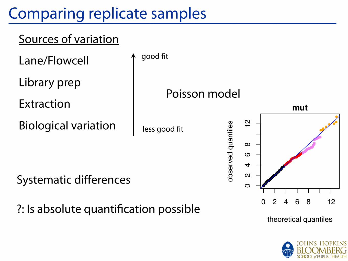
!
Comparing replicate samplesSources of variation
Lane/Flowcell
Library prep
Extraction
Biological variation
Poisson model
good !t
less good !t
Systematic differences
?: Is absolute quanti#cation possible
Analysis
!!!!!!!!!!!!!!!!!!!!!!!!!!!!!!!!!!!!!!!!!!!!!!!!!!!!!!!!!!!!!!!!!!!!!!!!!!!!!!!!!!!!!!!!!!!!!!!!!!!!!!!!!!!!!!!!!!!!!!!!!!!!!!!!!!!!!!!!!!!!!!!!!!!!!!!!!!!!!!!!!!!!!!!!!!!!!!!!!!!!!!!!!!!!!!!!!!!!!!!!!!!!!!!!!!!!!!!!!!!!!!!!!!!!!!!!!!!!!!!!!!!!!!!!!!!!!!!!!!!!!!!!!!!!!!!!!!!!!!!!!!!!!!!!!!!!!!!!!!!!!!!!!!!!!!!!!!!!!!!!!!!!!!!!!!!!!!!!!!!!!!!!!!!!!!!!!!!!!!!!!!!!!!!!!!!!!!!!!!!!!!!!!!!!!!!!!!!!!!!!!!!!!!!!!!!!!!!!!!!!!!!!!!!!!!!!!!!!!!!!!!!!!!!!!!!!!!!!!!!!!!!!!!!!!!!!!!!!!!!!!!!!!!!!!!!!!!!!!!!!!!!!!!!!!!!!!!!!!!!!!!!!!!!!!!!!!!!!!!!!!!!!!!!!!!!!!!!!!!!!!!!!!!!!!!!!!!!!!!!!!!!!!!!!!!!!!!!!!!!!!!!!!!!!!!!!!!!!!!!!!!!!!!!!!!!!!!!!!!!!!!!!!!!!!!!!!!!!!!!!!!!!!!!!!!!!!!!!!!!!!!!!!!!!!!!!!!!!!!!!!!!!!!!!!!!!!!!!!!!!!!!!!!!!!!!!!!!!!!!!!!!!!!!!!!!!!!!!!!!!!!!!!!!!!!!!!!!!!!!!!!!!!!!!!!!!!!!!!!!!!!!!!!!!!!!!!!!!!!!!!!!!!!!!!!!!!!!!!!!!!!!!!!!!!!!!!!!!!!!!!!!!!!!!!!!!!!!!!!!!!!!!!!!!!!!!!!!!!!!!!!!!!!!!!!!!!!!!!!!!!!!!!!!!!!!!!!!!!!!!!!!!!!!!!!!!!!!!!!!!!!!!!!!!!!!!!!!!!!!!!!!!!!!!!!!!!!!!!!!!!!!!!!!!!!!!!!!!!!!!!!!!!!!!!!!!!!!!!!!!!!!!!!!!!!!!!!!!!!!!!!!!!!!!!!!!!!!!!!!!!!!!!!!!!!!!!!!!!!!!!!!!!!!!!!!!!!!!!!!!!!!!!!!!!!!!!!!!!!!!!!!!!!!!!!!!!!!!!!!!!!!!!!!!!!!!!!!!!!!!!!!!!!!!!!!!!!!!!!!!!!!!!!!!!!!!!!!!!!!!!!!!!!!!!!!!!!!!!!!!!!!!!!!!!!!!!!!!!!!!!!!!!!!!!!!!!!!!!!!!!!!!!!!!!!!!!!!!!!!!!!!!!!!!!!!!!!!!!!!!!!!!!!!!!!!!!!!!!!!!!!!!!!!!!!!!!!!!!!!!!!!!!!!!!!!!!!!!!!!!!!!!!!!!!!!!!!!!!!!!!!!!!!!!!!!!!!!!!!!!!!!!!!!!!!!!!!!!!!!!!!!!!!!!!!!!!!!!!!!!!!!!!!!!!!!!!!!!!!!!!!!!!!!!!!!!!!!!!!!!!!!!!!!!!!!!!!!!!!!!!!!!!!!!!!!!!!!!!!!!!!!!!!!!!!!!!!!!!!!!!!!!!!!!!!!!!!!!!!!!!!!!!!!!!!!!!!!!!!!!!!!!!!!!!!!!!!!!!!!!!!!!!!!!!!!!!!!!!!!!!!!!!!!!!!!!!!!!!!!!!!!!!!!!!!!!!!!!!!!!!!!!!!!!!!!!!!!!!!!!!!!!!!!!!!!!!!!!!!!!!!!!!!!!!!!!!!!!!!!!!!!!!!!!!!!!!!!!!!!!!!!!!!!!!!!!!!!!!!!!!!!!!!!!!!!!!!!!!!!!!!!!!!!!!!!!!!!!!!!!!!!!!!!!!!!!!!!!!!!!!!!!!!!!!!!!!!!!!!!!!!!!!!!!!!!!!!!!!!!!!!!!!!!!!!!!!!!!!!!!!!!!!!!!!!!!!!!!!!!!!!!!!!!!!!!!!!!!!!!!!!!!!!!!!!!!!!!!!!!!!!!!!!!!!!!!!!!!!!!!!!!!!!!!!!!!!!!!!!!!!!!!!!!!!!!!!!!!!!!!!!!!!!!!!!!!!!!!!!!!!!!!!!!!!!!!!!!!!!!!!!!!!!!!!!!!!!!!!!!!!!!!!!!!!!!!!!!!!!!!!!!!!!!!!!!!!!!!!!!!!!!!!!!!!!!!!!!!!!!!!!!!!!!!!!!!!!!!!!!!!!!!!!!!!!!!!!!!!!!!!!!!!!!!!!!!!!!!!!!!!!!!!!!!!!!!!!!!!!!!!!!!!!!!!!!!!!!!!!!!!!!!!!!!!!!!!!!!!!!!!!!!!!!!!!!!!!!!!!!!!!!!!!!!!!!!!!!!!!!!!!!!!!!!!!!!!!!!!!!!!!!!!!!!!!!!!!!!!!!!!!!!!!!!!!!!!!!!!!!!!!!!!!!!!!!!!!!!!!!!!!!!!!!!!!!!!!!!!!!!!!!!!!!!!!!!!!!!!!!!!!!!!!!!!!!!!!!!!!!!!!!!!!!!!!!!!!!!!!!!!!!!!!!!!!!!!!!!!!!!!!!!!!!!!!!!!!!!!!!!!!!!!!!!!!!!!!!!!!!!!!!!!!!!!!!!!!!!!!!!!!!!!!!!!!!!!!!!!!!!!!!!!!!!!!!!!!!!!!!!!!!!!!!!!!!!!!!!!!!!!!!!!!!!!!!!!!!!!!!!!!!!!!!!!!!!!!!!!!!!!!!!!!!!!!!!!!!!!!!!!!!!!!!!!!!!!!!!!!!!!!!!!!!!!!!!!!!!!!!!!!!!!!!!!!!!!!!!!!!!!!!!!!!!!!!!!!!!!!!!!!!!!!!!!!!!!!!!!!!!!!!!!!!!!!!!!!!!!!!!!!!!!!!!!!!!!!!!!!!!!!!!!!!!!!!!!!!!!!!!!!!!!!!!!!!!!!!!!!!!!!!!!!!!!!!!!!!!!!!!!!!!!!!!!!!!!!!!!!!!!!!!!!!!!!!!!!!!!!!!!!!!!!!!!!!!!!!!!!!!!!!!!!!!!!!!!!!!!!!!!!!!!!!!!!!!!!!!!!!!!!!!!!!!!!!!!!!!!!!!!!!!!!!!!!!!!!!!!!!!!!!!!!!!!!!!!!!!!!!!!!!!!!!!!!!!!!!!!!!!!!!!!!!!!!!!!!!!!!!!!!!!!!!!!!!!!!!!!!!!!!!!!!!!!!!!!!!!!!!!!!!!!!!!!!!!!!!!!!!!!!!!!!!!!!!!!!!!!!!!!!!!!!!!!!!!!!!!!!!!!!!!!!!!!!!!!!!!!!!!!!!!!!!!!!!!!!!!!!!!!!!!!!!!!!!!!!!!!!!!!!!!!!!!!!!!!!!!!!!!!!!!!!!!!!!!!!!!!!!!!!!!!!!!!!!!!!!!!!!!!!!!!!!!!!!!!!!!!!!!!!!!!!!!!!!!!!!!!!!!!!!!!!!!!!!!!!!!!!!!!!!!!!!!!!!!!!!!!!!!!!!!!!!!!!!!!!!!!!!!!!!!!!!!!!!!!!!!!!!!!!!!!!!!!!!!!!!!!!!!!!!!!!!!!!!!!!!!!!!!!!!!!!!!!!!!!!!!!!!!!!!!!!!!!!!!!!!!!!!!!!!!!!!!!!!!!!!!!!!!!!!!!!!!!!!!!!!!!!!!!!!!!!!!!!!!!!!!!!!!!!!!!!!!!!!!!!!!!!!!!!!!!!!!!!!!!!!!!!!!!!!!!!!!!!!!!!!!!!!!!!!!!!!!!!!!!!!!!!!!!!!!!!!!!!!!!!!!!!!!!!!!!!!!!!!!!!!!!!!!!!!!!!!!!!!!!!!!!!!!!!!!!!!!!!!!!!!!!!!!!!!!!!!!!!!!!!!!!!!!!!!!!!!!!!!!!!!!!!!!!!!!!!!!!!!!!!!!!!!!!!!!!!!!!!!!!!!!!!!!!!!!!!!!!!!!!!!!!!!!!!!!!!!!!!!!!!!!!!!!!!!!!!!!!!!!!!!!!!!!!!!!!!!!!!!!!!!!!!!!!!!!!!!!!!!!!!!!!!!!!!!!!!!!!!!!!!!!!!!!!!!!!!!!!!!!!!!!!!!!!!!!!!!!!!!!!!!!!!!!!!!!!!!!!!!!!!!!!!!!!!!!!!!!!!!!!!!!!!!!!!!!!!!!!!!!!!!!!!!!!!!!!!!!!!!!!!!!!!!!!!!!!!!!!!!!!!!!!!!!!!!!!!!!!!!!!!!!!!!!!!!!!!!!!!!!!!!!!!!!!!!!!!!!!!!!!!!!!!!!!!!!!!!!!!!!!!!!!!!!!!!!!!!!!!!!!!!!!!!!!!!!!!!!!!!!!!!!!!!!!!!!!!!!!!!!!!!!!!!!!!!!!!!!!!!!!!!!!!!!!!!!!!!!!!!!!!!!!!!!!!!!!!!!!!!!!!!!!!!!!!!!!!!!!!!!!!!!!!!!!!!!!!!!!!!!!!!!!!!!!!!!!!!!!!!!!!!!!!!!!!!!!!!!!!!!!!!!!!!!!!!!!!!!!!!!!!!!!!!!!!!!!!!!!!!!!!!!!!!!!!!!!!!!!!!!!!!!!!!!!!!!!!!!!!!!!!!!!!!!!!!!!!!!!!!!!!!!!!!!!!!!!!!!!!!!!!!!!!!!!!!!!!!!!!!!!!!!!!!!!!!!!!!!!!!!!!!!!!!!!!!!!!!!!!!!!!!!!!!!!!!!!!!!!!!!!!!!!!!!!!!!!!!!!!!!!!!!!!!!!!!!!!!!!!!!!!!!!!!!!!!!!!!!!!!!!!!!!!!!!!!!!!!!!!!!!!!!!!!!!!!!!!!!!!!!!!!!!!!!!!!!!!!!!!!!!!!!!!!!!!!!!!!!!!!!!!!!!!!!!!!!!!!!!!!!!!!!!!!!!!!!!!!!!!!!!!!!!!!!!!!!!!!!!!!!!!!!!!!!!!!!!!!!!!!!!!!!!!!!!!!!!!!!!!!!!!!!!!!!!!!!!!!!!!!!!!!!!!!!!!!!!!!!!!!!!!!!!!!!!!!!!!!!!!!!!!!!!!!!!!!!!!!!!!!!!!!!!!!!!!!!!!!!!!!!!!!!!!!!!!!!!!!!!!!!!!!!!!!!!!!!!!!!!!!!!!!!!!!!!!!!!!!!!!!!!!!!!!!!!!!!!!!!!!!!!!!!!!!!!!!!!!!!!!!!!!!!!!!!!!!!!!!!!!!!!!!!!!!!!!!!!!!!!!!!!!!!!!!!!!!!!!!!!!!!!!!!!!!!!!!!!!!!!!!!!!!!!!!!!!!!!!!!!!!!!!!!!!!!!!!!!!!!!!!!!!!!!!!!!!!!!!!!!!!!!!!!!!!!!!!!!!!!!!!!!!!!!!!!!!!!!!!!!!!!!!!!!!!!!!!!!!!!!!!!!!!!!!!!!!!!!!!!!!!!!!!!!!!!!!!!!!!!!!!!!!!!!!!!!!!!!!!!!!!!!!!!!!!!!!!!!!!!!!!!!!!!!!!!!!!!!!!!!!!!!!!!!!!!!!!!!!!!!!!!!!!!!!!!!!!!!!!!!!!!!!!!!!!!!!!!!!!!!!!!!!!!!!!!!!!!!!!!!!!!!!!!!!!!!!!!!!!!!!!!!!!!!!!!!!!!!!!!!!!!!!!!!!!!!!!!!!!!!!!!!!!!!!!!!!!!!!!!!!!!!!!!!!!!!!!!!!!!!!!!!!!!!!!!!!!!!!!!!!!!!!!!!!!!!!!!!!!!!!!!!!!!!!!!!!!!!!!!!!!!!!!!!!!!!!!!!!!!!!!!!!!!!!!!!!!!!!!!!!!!!!!!!!!!!!!!!!!!!!!!!!!!!!!!!!!!!!!!!!!!!!!!!!!!!!!!!!!!!!!!!!!!!!!!!!!!!!!!!!!!!!!!!!!!!!!!!!!!!!!!!!!!!!!!!!!!!!!!!!!!!!!!!!!!!!!!!!!!!!!!!!!!!!!!!!!!!!!!!!!!!!!!!!!!!!!!!!!!!!!!!!!!!!!!!!!!!!!!!!!!!!!!!!!!!!!!!!!!!!!!!!!!!!!!!!!!!!!!!!!!!!!!!!!!!!!!!!!!!!!!!!!!!!!!!!!!!!!!!!!!!!!!!!!!!!!!!!!!!!!!!!!!!!!!!!!!!!!!!!!!!!!!!!!!!!!!!!!!!!!!!!!!!!!!!!!!!!!!!!!!!!!!!!!!!!!!!!!!!!!!!!!!!!!!!!!!!!!!!!!!!!!!!!!!!!!!!!!!!!!!!!!!!!!!!!!!!!!!!!!!!!!!!!!!!!!!!!!!!!!!!!!!!!!!!!!!!!!!!!!!!!!!!!!!!!!!!!!!!!!!!!!!!!!!!!!!!!!!!!!!!!!!!!!!!!!!!!!!!!!!!!!!!!!!!!!!!!!!!!!!!!!!!!!!!!!!!!!!!!!!!!!!!!!!!!!!!!!!!!!!!!!!!!!!!!!!!!!!!!!!!!!!!!!!!!!!!!!!!!!!!!!!!!!!!!!!!!
!!!!!!!!!!!!!!!!!!!!!!!
!!!!! !
!
!
0 2 4 6 8 12
02
46
812
mut
theoretical quantiles
observ
ed q
uantile
s
!!!!!!!!!!!!!!!!!!!!!!!!!!!!!!!!!!!!!!!!!!!!!!!!!!!!!!!!!!!!!!!!!!!!!!!!!!!!!!!!!!!!!!!!!!!!!!!!!!!!!!!!!!!!!!!!!!!!!!!!!!!!!!!!!!!!!!!!!!!!!!!!!!!!!!!!!!!!!!!!!!!!!!!!!!!!!!!!!!!!!!!!!!!!!!!!!!!!!!!!!!!!!!!!!!!!!!!!!!!!!!!!!!!!!!!!!!!!!!!!!!!!!!!!!!!!!!!!!!!!!!!!!!!!!!!!!!!!!!!!!!!!!!!!!!!!!!!!!!!!!!!!!!!!!!!!!!!!!!!!!!!!!!!!!!!!!!!!!!!!!!!!!!!!!!!!!!!!!!!!!!!!!!!!!!!!!!!!!!!!!!!!!!!!!!!!!!!!!!!!!!!!!!!!!!!!!!!!!!!!!!!!!!!!!!!!!!!!!!!!!!!!!!!!!!!!!!!!!!!!!!!!!!!!!!!!!!!!!!!!!!!!!!!!!!!!!!!!!!!!!!!!!!!!!!!!!!!!!!!!!!!!!!!!!!!!!!!!!!!!!!!!!!!!!!!!!!!!!!!!!!!!!!!!!!!!!!!!!!!!!!!!!!!!!!!!!!!!!!!!!!!!!!!!!!!!!!!!!!!!!!!!!!!!!!!!!!!!!!!!!!!!!!!!!!!!!!!!!!!!!!!!!!!!!!!!!!!!!!!!!!!!!!!!!!!!!!!!!!!!!!!!!!!!!!!!!!!!!!!!!!!!!!!!!!!!!!!!!!!!!!!!!!!!!!!!!!!!!!!!!!!!!!!!!!!!!!!!!!!!!!!!!!!!!!!!!!!!!!!!!!!!!!!!!!!!!!!!!!!!!!!!!!!!!!!!!!!!!!!!!!!!!!!!!!!!!!!!!!!!!!!!!!!!!!!!!!!!!!!!!!!!!!!!!!!!!!!!!!!!!!!!!!!!!!!!!!!!!!!!!!!!!!!!!!!!!!!!!!!!!!!!!!!!!!!!!!!!!!!!!!!!!!!!!!!!!!!!!!!!!!!!!!!!!!!!!!!!!!!!!!!!!!!!!!!!!!!!!!!!!!!!!!!!!!!!!!!!!!!!!!!!!!!!!!!!!!!!!!!!!!!!!!!!!!!!!!!!!!!!!!!!!!!!!!!!!!!!!!!!!!!!!!!!!!!!!!!!!!!!!!!!!!!!!!!!!!!!!!!!!!!!!!!!!!!!!!!!!!!!!!!!!!!!!!!!!!!!!!!!!!!!!!!!!!!!!!!!!!!!!!!!!!!!!!!!!!!!!!!!!!!!!!!!!!!!!!!!!!!!!!!!!!!!!!!!!!!!!!!!!!!!!!!!!!!!!!!!!!!!!!!!!!!!!!!!!!!!!!!!!!!!!!!!!!!!!!!!!!!!!!!!!!!!!!!!!!!!!!!!!!!!!!!!!!!!!!!!!!!!!!!!!!!!!!!!!!!!!!!!!!!!!!!!!!!!!!!!!!!!!!!!!!!!!!!!!!!!!!!!!!!!!!!!!!!!!!!!!!!!!!!!!!!!!!!!!!!!!!!!!!!!!!!!!!!!!!!!!!!!!!!!!!!!!!!!!!!!!!!!!!!!!!!!!!!!!!!!!!!!!!!!!!!!!!!!!!!!!!!!!!!!!!!!!!!!!!!!!!!!!!!!!!!!!!!!!!!!!!!!!!!!!!!!!!!!!!!!!!!!!!!!!!!!!!!!!!!!!!!!!!!!!!!!!!!!!!!!!!!!!!!!!!!!!!!!!!!!!!!!!!!!!!!!!!!!!!!!!!!!!!!!!!!!!!!!!!!!!!!!!!!!!!!!!!!!!!!!!!!!!!!!!!!!!!!!!!!!!!!!!!!!!!!!!!!!!!!!!!!!!!!!!!!!!!!!!!!!!!!!!!!!!!!!!!!!!!!!!!!!!!!!!!!!!!!!!!!!!!!!!!!!!!!!!!!!!!!!!!!!!!!!!!!!!!!!!!!!!!!!!!!!!!!!!!!!!!!!!!!!!!!!!!!!!!!!!!!!!!!!!!!!!!!!!!!!!!!!!!!!!!!!!!!!!!!!!!!!!!!!!!!!!!!!!!!!!!!!!!!!!!!!!!!!!!!!!!!!!!!!!!!!!!!!!!!!!!!!!!!!!!!!!!!!!!!!!!!!!!!!!!!!!!!!!!!!!!!!!!!!!!!!!!!!!!!!!!!!!!!!!!!!!!!!!!!!!!!!!!!!!!!!!!!!!!!!!!!!!!!!!!!!!!!!!!!!!!!!!!!!!!!!!!!!!!!!!!!!!!!!!!!!!!!!!!!!!!!!!!!!!!!!!!!!!!!!!!!!!!!!!!!!!!!!!!!!!!!!!!!!!!!!!!!!!!!!!!!!!!!!!!!!!!!!!!!!!!!!!!!!!!!!!!!!!!!!!!!!!!!!!!!!!!!!!!!!!!!!!!!!!!!!!!!!!!!!!!!!!!!!!!!!!!!!!!!!!!!!!!!!!!!!!!!!!!!!!!!!!!!!!!!!!!!!!!!!!!!!!!!!!!!!!!!!!!!!!!!!!!!!!!!!!!!!!!!!!!!!!!!!!!!!!!!!!!!!!!!!!!!!!!!!!!!!!!!!!!!!!!!!!!!!!!!!!!!!!!!!!!!!!!!!!!!!!!!!!!!!!!!!!!!!!!!!!!!!!!!!!!!!!!!!!!!!!!!!!!!!!!!!!!!!!!!!!!!!!!!!!!!!!!!!!!!!!!!!!!!!!!!!!!!!!!!!!!!!!!!!!!!!!!!!!!!!!!!!!!!!!!!!!!!!!!!!!!!!!!!!!!!!!!!!!!!!!!!!!!!!!!!!!!!!!!!!!!!!!!!!!!!!!!!!!!!!!!!!!!!!!!!!!!!!!!!!!!!!!!!!!!!!!!!!!!!!!!!!!!!!!!!!!!!!!!!!!!!!!!!!!!!!!!!!!!!!!!!!!!!!!!!!!!!!!!!!!!!!!!!!!!!!!!!!!!!!!!!!!!!!!!!!!!!!!!!!!!!!!!!!!!!!!!!!!!!!!!!!!!!!!!!!!!!!!!!!!!!!!!!!!!!!!!!!!!!!!!!!!!!!!!!!!!!!!!!!!!!!!!!!!!!!!!!!!!!!!!!!!!!!!!!!!!!!!!!!!!!!!!!!!!!!!!!!!!!!!!!!!!!!!!!!!!!!!!!!!!!!!!!!!!!!!!!!!!!!!!!!!!!!!!!!!!!!!!!!!!!!!!!!!!!!!!!!!!!!!!!!!!!!!!!!!!!!!!!!!!!!!!!!!!!!!!!!!!!!!!!!!!!!!!!!!!!!!!!!!!!!!!!!!!!!!!!!!!!!!!!!!!!!!!!!!!!!!!!!!!!!!!!!!!!!!!!!!!!!!!!!!!!!!!!!!!!!!!!!!!!!!!!!!!!!!!!!!!!!!!!!!!!!!!!!!!!!!!!!!!!!!!!!!!!!!!!!!!!!!!!!!!!!!!!!!!!!!!!!!!!!!!!!!!!!!!!!!!!!!!!!!!!!!!!!!!!!!!!!!!!!!!!!!!!!!!!!!!!!!!!!!!!!!!!!!!!!!!!!!!!!!!!!!!!!!!!!!!!!!!!!!!!!!!!!!!!!!!!!!!!!!!!!!!!!!!!!!!!!!!!!!!!!!!!!!!!!!!!!!!!!!!!!!!!!!!!!!!!!!!!!!!!!!!!!!!!!!!!!!!!!!!!!!!!!!!!!!!!!!!!!!!!!!!!!!!!!!!!!!!!!!!!!!!!!!!!!!!!!!!!!!!!!!!!!!!!!!!!!!!!!!!!!!!!!!!!!!!!!!!!!!!!!!!!!!!!!!!!!!!!!!!!!!!!!!!!!!!!!!!!!!!!!!!!!!!!!!!!!!!!!!!!!!!!!!!!!!!!!!!!!!!!!!!!!!!!!!!!!!!!!!!!!!!!!!!!!!!!!!!!!!!!!!!!!!!!!!!!!!!!!!!!!!!!!!!!!!!!!!!!!!!!!!!!!!!!!!!!!!!!!!!!!!!!!!!!!!!!!!!!!!!!!!!!!!!!!!!!!!!!!!!!!!!!!!!!!!!!!!!!!!!!!!!!!!!!!!!!!!!!!!!!!!!!!!!!!!!!!!!!!!!!!!!!!!!!!!!!!!!!!!!!!!!!!!!!!!!!!!!!!!!!!!!!!!!!!!!!!!!!!!!!!!!!!!!!!!!!!!!!!!!!!!!!!!!!!!!!!!!!!!!!!!!!!!!!!!!!!!!!!!!!!!!!!!!!!!!!!!!!!!!!!!!!!!!!!!!!!!!!!!!!!!!!!!!!!!!!!!!!!!!!!!!!!!!!!!!!!!!!!!!!!!!!!!!!!!!!!!!!!!!!!!!!!!!!!!!!!!!!!!!!!!!!!!!!!!!!!!!!!!!!!!!!!!!!!!!!!!!!!!!!!!!!!!!!!!!!!!!!!!!!!!!!!!!!!!!!!!!!!!!!!!!!!!!!!!!!!!!!!!!!!!!!!!!!!!!!!!!!!!!!!!!!!!!!!!!!!!!!!!!!!!!!!!!!!!!!!!!!!!!!!!!!!!!!!!!!!!!!!!!!!!!!!!!!!!!!!!!!!!!!!!!!!!!!!!!!!!!!!!!!!!!!!!!!!!!!!!!!!!!!!!!!!!!!!!!!!!!!!!!!!!!!!!!!!!!!!!!!!!!!!!!!!!!!!!!!!!!!!!!!!!!!!!!!!!!!!!!!!!!!!!!!!!!!!!!!!!!!!!!!!!!!!!!!!!!!!!!!!!!!!!!!!!!!!!!!!!!!!!!!!!!!!!!!!!!!!!!!!!!!!!!!!!!!!!!!!!!!!!!!!!!!!!!!!!!!!!!!!!!!!!!!!!!!!!!!!!!!!!!!!!!!!!!!!!!!!!!!!!!!!!!!!!!!!!!!!!!!!!!!!!!!!!!!!!!!!!!!!!!!!!!!!!!!!!!!!!!!!!!!!!!!!!!!!!!!!!!!!!!!!!!!!!!!!!!!!!!!!!!!!!!!!!!!!!!!!!!!!!!!!!!!!!!!!!!!!!!!!!!!!!!!!!!!!!!!!!!!!!!!!!!!!!!!!!!!!!!!!!!!!!!!!!!!!!!!!!!!!!!!!!!!!!!!!!!!!!!!!!!!!!!!!!!!!!!!!!!!!!!!!!!!!!!!!!!!!!!!!!!!!!!!!!!!!!!!!!!!!!!!!!!!!!!!!!!!!!!!!!!!!!!!!!!!!!!!!!!!!!!!!!!!!!!!!!!!!!!!!!!!!!!!!!!!!!!!!!!!!!!!!!!!!!!!!!!!!!!!!!!!!!!!!!!!!!!!!!!!!!!!!!!!!!!!!!!!!!!!!!!!!!!!!!!!!!!!!!!!!!!!!!!!!!!!!!!!!!!!!!!!!!!!!!!!!!!!!!!!!!!!!!!!!!!!!!!!!!!!!!!!!!!!!!!!!!!!!!!!!!!!!!!!!!!!!!!!!!!!!!!!!!!!!!!!!!!!!!!!!!!!!!!!!!!!!!!!!!!!!!!!!!!!!!!!!!!!!!!!!!!!!!!!!!!!!!!!!!!!!!!!!!!!!!!!!!!!!!!!!!!!!!!!!!!!!!!!!!!!!!!!!!!!!!!!!!!!!!!!!!!!!!!!!!!!!!!!!!!!!!!!!!!!!!!!!!!!!!!!!!!!!!!!!!!!!!!!!!!!!!!!!!!!!!!!!!!!!!!!!!!!!!!!!!!!!!!!!!!!!!!!!!!!!!!!!!!!!!!!!!!!!!!!!!!!!!!!!!!!!!!!!!!!!!!!!!!!!!!!!!!!!!!!!!!!!!!!!!!!!!!!!!!!!!!!!!!!!!!!!!!!!!!!!!!!!!!!!!!!!!!!!!!!!!!!!!!!!!!!!!!!!!!!!!!!!!!!!!!!!!!!!!!!!!!!!!!!!!!!!!!!!!!!!!!!!!!!!!!!!!!!!!!!!!!!!!!!!!!!!!!!!!!!!!!!!!!!!!!!!!!!!!!!!!!!!!!!!!!!!!!!!!!!!!!!!!!!!!!!!!!!!!!!!!!!!!!!!!!!!!!!!!!!!!!!!!!!!!!!!!!!!!!!!!!!!!!!!!!!!!!!!!!!!!!!!!!!!!!!!!!!!!!!!!!!!!!!!!!!!!!!!!!!!!!!!!!!!!!!!!!!!!!!!!!!!!!!!!!!!!!!!!!!!!!!!!!!!!!!!!!!!!!!!!!!!!!!!!!!!!!!!!!!!!!!!!!!!!!!!!!!!!!!!!!!!!!!!!!!!!!!!!!!!!!!!!!!!!!!!!!!!!!!!!!!!!!!!!!!!!!!!!!!!!!!!!!!!!!!!!!!!!!!!!!!!!!!!!!!!!!!!!!!!!!!!!!!!!!!!!!!!!!!!!!!!!!!!!!!!!!!!!!!!!!!!!!!!!!!!!!!!!!!!!!!!!!!!!!!!!!!!!!!!!!!!!!!!!!!!!!!!!!!!!!!!!!!!!!!!!!!!!!!!!!!!!!!!!!!!!!!!!!!
!!!
!!!!!!
!
0 5 10 15
05
10
15
wt
theoretical quantiles
observ
ed q
uantile
s
> plot(regionGoodnessOfFit(geneCountsUI, groups = rep("all",
+ 4)), chisq = TRUE)
41 / 40
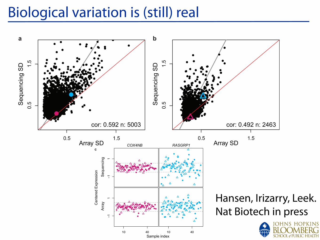
!
Biological variation is (still) real! "
!"#$%&'()*%+$%*(,-
.##/0%12
13453+!6+7%12
&'8
9'8
&'8 9'8
!"#$%&'8)*%+$%8&&-
.##/0%12
13453+!6+7%12
&'8
9'8
&'8 9'8
!
!
!
!"#$%&'()*&+
,&)-&.&*'/+$.&00(1)
!&23&)4()5
6.."7
!"#$%& '()*'+,
!
!
!
!
!!!!!!
!!
!!!
!!
!!!!!!
!!
!!!!!!
!!!
!
!
!
!!
!!
!!!
!
!!!!!!
!
!
!!!
!
!!!
!
!!
!
!
!!
!
!
!
!
!
!
!
!
!
!!
!
!!
!
!!!
!
!
!
!
!!
!
!
!
!
!
!!
!!
!
!
!
!
!!
!
!!!!!!
!!!!
!
!!!!!
!
!!
!
!
!
!
!
!!
!!!!!
!!!!!
!
!
!!!!!!
!
!!
!
!!
!!
!
!!
!
!
!
!
!
!
!!!
!
!
!!
!
!!
!
!
!
!
!!
!
!!
!
!
!!!
!!
!
!
!
!
!!
!
!!
!
Hansen, Irizarry, Leek. Nat Biotech in press
!
Differential Expression, ConclusionStill need normalization
Methods for DE are appearing
Anders, S. & Huber, W. Differential expression analysis for sequence count data. Genome Biol 11, R106 (2010).
Bullard, J.H., Purdom, E., Hansen, K.D. & Dudoit, S. Evaluation of statistical methods for normalization and differential expression in mRNA-Seq experiments. BMC Bioinformatics 11, 94 (2010).
Langmead, B., Hansen, K.D. & Leek, J.T. Cloud-scale RNA-sequencing differential expression analysis with Myrna. Genome Biol 11, R83 (2010).
Oshlack, A., Robinson, M.D. & Young, M.D. From RNA-seq reads to differential expression results. Genome Biol 11, 220 (2010).
Oshlack, A. & Wakefield, M.J. Transcript length bias in RNA-seq data confounds systems biology. Biol. Direct 4, 14 (2009).
Robinson, M.D. & Oshlack, A. A scaling normalization method for differential expression analysis of RNA-seq data. Genome Biol 11, R25 (2010).