Roadside measurement and prediction of CO and PM2.5 dispersion from on-road vehicles in Hong Kong

Transportation Research Part D 11 (2006) 242–249

www.elsevier.com/locate/trd

Roadside measurement and prediction of CO and PM2.5

dispersion from on-road vehicles in Hong Kong

J.S. Wang a, T.L. Chan a,*, Z. Ning a, C.W. Leung a, C.S. Cheung a, W.T. Hung b

a Research Centre for Combustion and Pollution Control, Department of Mechanical Engineering,

The Hong Kong Polytechnic University, Hung Hom, Kowloon, Hong Kongb Department of Civil and Structural Engineering, The Hong Kong Polytechnic University, Hung Hom, Kowloon, Hong Kong

Abstract

This study investigates the traffic induced gaseous and particle emissions dispersion characteristics from the typicalurban roadside sites in Hong Kong. Concentrations of carbon monoxide, CO, fine particles, PM2.5 pollutants, and the traf-fic and ambient atmospheric conditions at three selected local urban road sites were simultaneously measured. A developedlocal general finite line source model (GFLSM) was used to predict the local roadside CO and fine particle concentrations.A high level of agreement found between the measured and calculated CO and PM2.5 data. Generally, the roadside con-centrations of gaseous and PM2.5 pollutants decrease with the distance away from the road and the exposure to both gas-eous and particle pollutants in the vicinity of the selected urban road sites is interrelated to on-road vehicle emissions. Ithas also demonstrated that the developed local general finite line source model has the capability of reasonably predictingthe characteristics of gaseous and particle pollutant dispersion from on-road vehicles for the local urban air quality.� 2006 Elsevier Ltd. All rights reserved.

Keywords: Finite line source dispersion model; Particulate matter, PM2.5; Carbon monoxide; On-road vehicles; Field measurement

1. Introduction

Motor vehicle emissions are the major source of air pollution problem in most urban cities. Many modelshave been developed and applied to simulate the line source emission dispersion in the rural open highway,such as the General Motors (GM) line source model (Chock, 1978), California line (CALINE) source models(Benson, 1979) and Highway (HIWAY) air pollution models (Zimmerman and Thompson, 1975). Luhar andPatil (1989) presented a general finite line source model (GFLSM) for all wind directions based on the Gauss-ian diffusion equations. The prediction performance of GFLSM was compared with GM, CALINE-3 andHIWAY-2 models and a reasonable accuracy for the Indian traffic conditions was shown (Sharma and Khare,2001; Nagendra and Khare, 2002). In the present study, a local GFLSM model has been developed for sim-ulating the CO and fine particle dispersion from the selected urban road sites in Hong Kong.

1361-9209/$ - see front matter � 2006 Elsevier Ltd. All rights reserved.

doi:10.1016/j.trd.2006.04.002

* Corresponding author. Tel.: +852 2766 6656; fax: +852 2365 4703.E-mail address: [email protected] (T.L. Chan).

mailto:[email protected]

J.S. Wang et al. / Transportation Research Part D 11 (2006) 242–249 243

2. The general finite line source model

2.1. GFLSM model equation for gaseous pollutant dispersion

For the prediction of traffic-induced gaseous pollutants, the developed line source model is based on theclassical GFLSM (Luhar and Patil, 1989) and the GM line source model (Chock, 1978). Luhar and Patil(1989) first developed the GFLSM by using the coordinate transformation between the wind and the linesource coordinate systems as:

C ¼ Q

2ffiffiffiffiffiffi2pp

rzue

exp �ðz� heÞ2

2r2z

!þ exp �ðzþ heÞ2

2r2z

!" #

� erfsin hðL=2� yÞ � x cos hffiffiffi

2p

ry

!þ erf

sin hðL=2þ yÞ þ x cos hffiffiffi2p

ry

!" #ð1Þ

where C is the concentration (mg m�3 or ppm); Q, the line source strength per unit length (mg m�1 s�1 orm3 m�1 s�1); ry and rz are the horizontal and vertical dispersion parameters (m), respectively; ue = u sinh + u0 where u, the mean ambient wind speed (m s�1) at a specific source height; u0, the wind speed correctiondue to the traffic wake. A constant numerical value, u0 = 0.2 ms�1 is applied for the calculation; h is the anglebetween the roadway and wind direction; he = h + hp is the effective source height, where h, the line sourceheight (m) and hp is the plume rise (m); L, the line source length (m).

2.2. GFLSM model equation for particle pollutant dispersion

For the prediction of traffic-induced particle pollutants, the particle settling velocity needs to be consideredbut the reflection at the earth’s surface is ignored. This is because gravity has a greater effect on the particles/particulates movement than the gaseous pollutants one (Luhar and Patil, 1989). The basic equations of thedeveloped model for particle emissions prediction is:

C ¼XN

i¼1

wiQ


rzue

exp �z� he � V ti x

ð�uþu0ÞðAþB sin hÞ

� �h i2

2r2z

8><>:

9>=>;

264

375


2p

ry

( )þ erf


ry

( )" #ð2Þ

where N is the number of particle size classes; V ti , the settling velocity corresponding to the average particlesize of the ith class; wi, the weight fraction of particulates in the ith size class; the coefficients of A and B arestability dependent which are available from the GM line source model (Chock, 1978).

Assuming the particulate matters to be spherical, the settling velocity, Vt of the particle can be determinedas:

V t ¼

ffiffiffiffiffiffiffiffiffiffiffiffiffiffiffiffiffiffiffiffiffiffiffiffiffiffiffiffiffi4Dpgðqp � qaÞ

3CDqa

sð3Þ

where Dp is the diameter of particle; g, the gravitational acceleration; qp, the density of particle; qa, the densityof the ambient air fluid; CD, the drag coefficient of particle; g, the gravitational acceleration. With the simpli-fied formula, for example for the laminar flow, CD can be obtained from the Stokes law.

The Reynolds number of particle can be determined by using the Archimedes number:

Ar ¼D3

pgqaðq� qaÞla

ð4Þ

244 J.S. Wang et al. / Transportation Research Part D 11 (2006) 242–249

When the Archimedes number, Ar < 1.83, the Reynolds number of particle, Rep can be calculated by

Rep ¼Ar18

ð5Þ

If the diameter of particle, Dp 6 2.5 lm, then the settling velocity of particle, V ti 6 0:0002 m s�1, so the termV ti x

ð�uþu0ÞðAþB sin hÞ in Eq. (2) can be neglected if the downwind distance, x is also small. In the present study, the

prediction dispersion of PM2.5 (i.e., Dp 6 2.5 lm) from the roadside can be simplified from Eq. (2) as:

C ¼XN

i¼1

wiQ


rzue

exp �ðz� heÞ2

2r2z

( )" #


2p

ry

( )þ erf


ry

( )" #ð6Þ

2.3. Dispersion parameters

The dispersion parameters are the function of the Monin–Obukhov length, the friction velocity and themixing height (instead of the discrete Pasquill classes). These parameters are computed using the meteorolog-ical pre-processing model.

The lateral and vertical dispersion parameters (ry and rz) can be written as:

r2y ¼ r2

ya þ r2y0; r2

z ¼ r2za þ r2

z0 ð7Þ

where the subscripts of a and 0 refer to atmospheric turbulence and traffic-originated turbulence, respectively.The atmospheric turbulence is evaluated at the effective distance from the line source and at the effectivesource height. The Pasquill parameters are determined from Pasquill, 1961. However, the vertical dispersionparameter for atmospheric turbulence can be determined from the GM line source model.

The dispersions due to the traffic-induced turbulence are:

rz0 ¼ 3:57� 0:53U c

ry0 ¼ 2rz0

U c ¼ 1:85u0:164 cos2 h ð8Þ

2.4. Determination of Monin–Obukhov length

Monin–Obukhov length, L, can be expressed as:

L ¼ T 2u2�

jgh�ð9Þ

where T2 is air temperature at the height of 2 m; j is von Karman constant, 0.41; u*, the friction velocity; andh*, a temperature scale for turbulent heat transfer. The u* and h* are determined from van Ulden (1978), andare then iterated when the single wind speed at z1 and the temperature difference at z3 and z2 are measured atthe selected local urban roadside site.

3. Traffic-induced air pollutants from on-road vehicles using the developed local GFLSM

The roadside measurements of traffic-induced CO and PM2.5 concentration data were collected continu-ously at several selected sampling points for a certain sampling period. The local meteorological data, suchas the ambient temperature, wind speed and direction at the roadside sites, were collected continuously asthe input parameters for the developed local GFLSM. Traffic information, including the average vehicle speedand the traffic flow rate from different vehicle categories during the sampling time interval, was also recorded.


3.1. Urban roadside experimental setup

The roadside measurements from the traffic-induced emissions were carried out at three selected local urbanroad sites, namely Lion Rock Tunnel (Kowloon entrance), New Territories, Site 1; Waterloo Road and Dur-ham Road crossroad area, Kowloon Tong, Site 2; Tai Po Road (near the parking lot area of Shatin JockeyClub), New Territories, Site 3. The selected roads are relatively open with no adjacent high buildings and thetraffic flow rate is relatively high and steady.

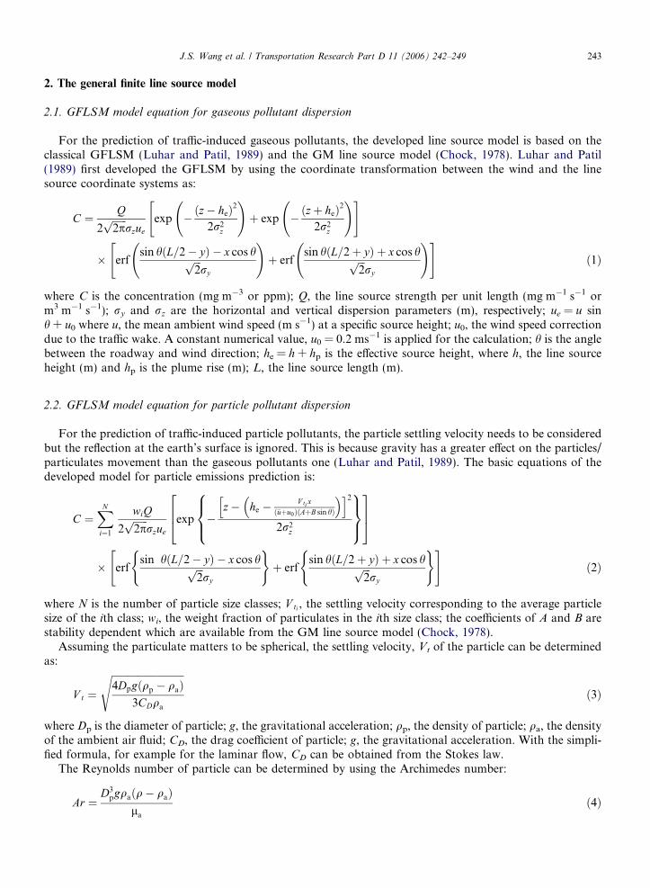
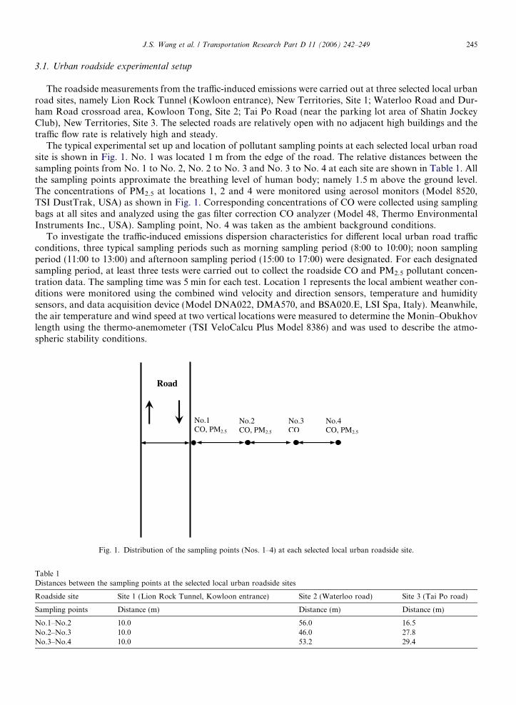
The typical experimental set up and location of pollutant sampling points at each selected local urban roadsite is shown in Fig. 1. No. 1 was located 1 m from the edge of the road. The relative distances between thesampling points from No. 1 to No. 2, No. 2 to No. 3 and No. 3 to No. 4 at each site are shown in Table 1. Allthe sampling points approximate the breathing level of human body; namely 1.5 m above the ground level.The concentrations of PM2.5 at locations 1, 2 and 4 were monitored using aerosol monitors (Model 8520,TSI DustTrak, USA) as shown in Fig. 1. Corresponding concentrations of CO were collected using samplingbags at all sites and analyzed using the gas filter correction CO analyzer (Model 48, Thermo EnvironmentalInstruments Inc., USA). Sampling point, No. 4 was taken as the ambient background conditions.

To investigate the traffic-induced emissions dispersion characteristics for different local urban road trafficconditions, three typical sampling periods such as morning sampling period (8:00 to 10:00); noon samplingperiod (11:00 to 13:00) and afternoon sampling period (15:00 to 17:00) were designated. For each designatedsampling period, at least three tests were carried out to collect the roadside CO and PM2.5 pollutant concen-tration data. The sampling time was 5 min for each test. Location 1 represents the local ambient weather con-ditions were monitored using the combined wind velocity and direction sensors, temperature and humiditysensors, and data acquisition device (Model DNA022, DMA570, and BSA020.E, LSI Spa, Italy). Meanwhile,the air temperature and wind speed at two vertical locations were measured to determine the Monin–Obukhovlength using the thermo-anemometer (TSI VeloCalcu Plus Model 8386) and was used to describe the atmo-spheric stability conditions.

No.1 CO, PM2.5

Road

No.2CO, PM2.5

No.3CO

No.4CO, PM2.5

Fig. 1. Distribution of the sampling points (Nos. 1–4) at each selected local urban roadside site.

Table 1Distances between the sampling points at the selected local urban roadside sites

Roadside site Site 1 (Lion Rock Tunnel, Kowloon entrance) Site 2 (Waterloo road) Site 3 (Tai Po road)

Sampling points Distance (m) Distance (m) Distance (m)

No.1–No.2 10.0 56.0 16.5No.2–No.3 10.0 46.0 27.8No.3–No.4 10.0 53.2 29.4

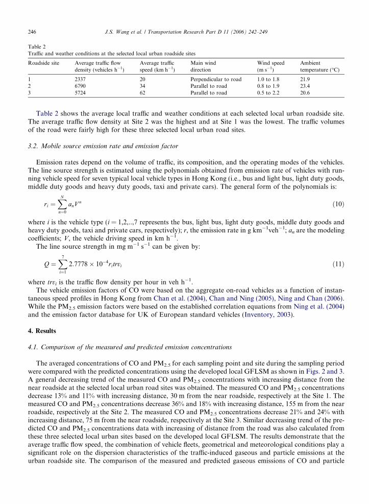
Table 2Traffic and weather conditions at the selected local urban roadside sites

Roadside site Average traffic flowdensity (vehicles h�1)

Average trafficspeed (km h�1)

Main winddirection

Wind speed(m s�1)

Ambienttemperature (�C)

1 2337 20 Perpendicular to road 1.0 to 1.8 21.92 6790 34 Parallel to road 0.8 to 1.9 23.43 5724 62 Parallel to road 0.5 to 2.2 20.6


Table 2 shows the average local traffic and weather conditions at each selected local urban roadside site.The average traffic flow density at Site 2 was the highest and at Site 1 was the lowest. The traffic volumesof the road were fairly high for these three selected local urban road sites.

3.2. Mobile source emission rate and emission factor

Emission rates depend on the volume of traffic, its composition, and the operating modes of the vehicles.The line source strength is estimated using the polynomials obtained from emission rate of vehicles with run-ning vehicle speed for seven typical local vehicle types in Hong Kong (i.e., bus and light bus, light duty goods,middle duty goods and heavy duty goods, taxi and private cars). The general form of the polynomials is:

ri ¼XN

n¼0

anV n ð10Þ

where i is the vehicle type (i = 1,2,..,7 represents the bus, light bus, light duty goods, middle duty goods andheavy duty goods, taxi and private cars, respectively); r, the emission rate in g km�1veh�1; an are the modelingcoefficients; V, the vehicle driving speed in km h�1.

The line source strength in mg m�1 s�1 can be given by:

Q ¼X7

i¼1

2:7778� 10�4ritrvi ð11Þ

where trvi is the traffic flow density per hour in veh h�1.The vehicle emission factors of CO were based on the aggregate on-road vehicles as a function of instan-

taneous speed profiles in Hong Kong from Chan et al. (2004), Chan and Ning (2005), Ning and Chan (2006).While the PM2.5 emission factors were based on the established correlation equations from Ning et al. (2004)and the emission factor database for UK of European standard vehicles (Inventory, 2003).

4. Results

4.1. Comparison of the measured and predicted emission concentrations

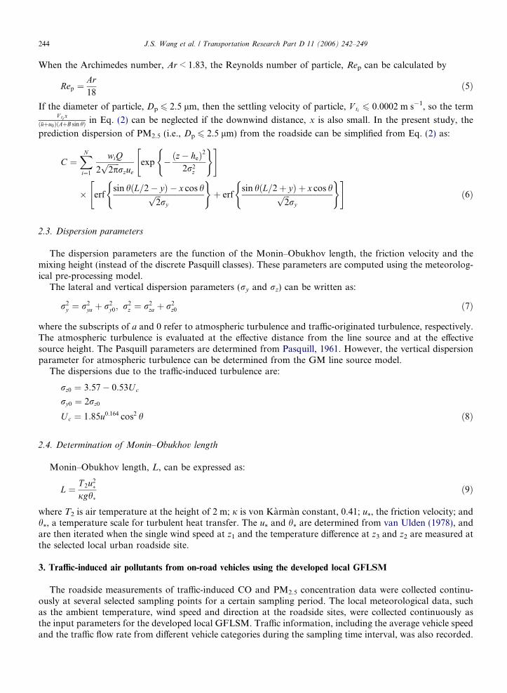
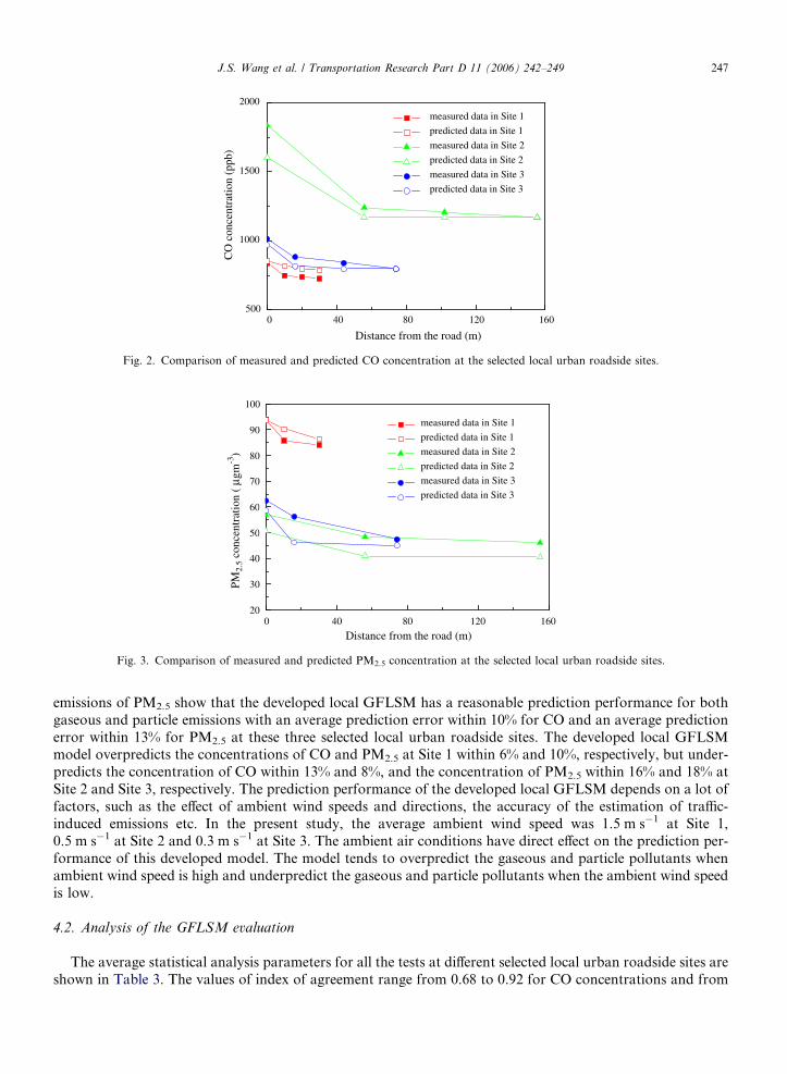
The averaged concentrations of CO and PM2.5 for each sampling point and site during the sampling periodwere compared with the predicted concentrations using the developed local GFLSM as shown in Figs. 2 and 3.A general decreasing trend of the measured CO and PM2.5 concentrations with increasing distance from thenear roadside at the selected local urban road sites was obtained. The measured CO and PM2.5 concentrationsdecrease 13% and 11% with increasing distance, 30 m from the near roadside, respectively at the Site 1. Themeasured CO and PM2.5 concentrations decrease 36% and 18% with increasing distance, 155 m from the nearroadside, respectively at the Site 2. The measured CO and PM2.5 concentrations decrease 21% and 24% withincreasing distance, 75 m from the near roadside, respectively at the Site 3. Similar decreasing trend of the pre-dicted CO and PM2.5 concentrations data with increasing of distance from the road was also calculated fromthese three selected local urban sites based on the developed local GFLSM. The results demonstrate that theaverage traffic flow speed, the combination of vehicle fleets, geometrical and meteorological conditions play asignificant role on the dispersion characteristics of the traffic-induced gaseous and particle emissions at theurban roadside site. The comparison of the measured and predicted gaseous emissions of CO and particle

0 40 80 120 160500

1000

1500

2000

measured data in Site 1

predicted data in Site 1





CO

con

cent

ratio

n (p

pb)

Distance from the road (m)

Fig. 2. Comparison of measured and predicted CO concentration at the selected local urban roadside sites.

0 40 80 120 16020

30

40

50

60

70

80

90

100







PM2.

5 co

ncen

trat

ion

(μg

m-3

)

Distance from the road (m)

Fig. 3. Comparison of measured and predicted PM2.5 concentration at the selected local urban roadside sites.


emissions of PM2.5 show that the developed local GFLSM has a reasonable prediction performance for bothgaseous and particle emissions with an average prediction error within 10% for CO and an average predictionerror within 13% for PM2.5 at these three selected local urban roadside sites. The developed local GFLSMmodel overpredicts the concentrations of CO and PM2.5 at Site 1 within 6% and 10%, respectively, but under-predicts the concentration of CO within 13% and 8%, and the concentration of PM2.5 within 16% and 18% atSite 2 and Site 3, respectively. The prediction performance of the developed local GFLSM depends on a lot offactors, such as the effect of ambient wind speeds and directions, the accuracy of the estimation of traffic-induced emissions etc. In the present study, the average ambient wind speed was 1.5 m s�1 at Site 1,0.5 m s�1 at Site 2 and 0.3 m s�1 at Site 3. The ambient air conditions have direct effect on the prediction per-formance of this developed model. The model tends to overpredict the gaseous and particle pollutants whenambient wind speed is high and underpredict the gaseous and particle pollutants when the ambient wind speedis low.

4.2. Analysis of the GFLSM evaluation

The average statistical analysis parameters for all the tests at different selected local urban roadside sites areshown in Table 3. The values of index of agreement range from 0.68 to 0.92 for CO concentrations and from

Table 3Average statistical parameters for model evaluation at the selected local urban roadside sites

Emissions (Unit) Site 1 Lion Rock Tunnel(Kowloon entrance)

Site 2 Waterloo road Site 3 Tai Po road

CO (ppb) PM2.5 (lg m�3) CO (ppb) PM2.5 (lg m�3) CO (ppb) PM2.5 (lg m�3)

Summary measures

Observed mean 762.1 88.0661 1362.9 50.4614 884.2 55.4177Predicted mean 814.4 90.2156 1203.8 44.0379 846.3 50.0092Observed deviation 45.0 4.3323 273.7 4.7229 84.4 6.1933Predicted deviation 25.4 3.0528 58.5 4.6322 73.1 6.2140

Linear regression

Intercept 0.4320 33.1293 0.8984 �6.7308 0.0441 2.6801Slope 0.5051 0.6546 0.2268 1.0163 0.9213 0.8585Correlation coefficient 0.9309 0.9032 0.9901 0.9625 0.9497 0.8472

Index of agreement 0.6791 0.5997 0.9189 0.7128 0.8400 0.7524


0.60 to 0.75 for PM2.5 concentrations. All of these values correspond to a fairly good agreement between thepredicted and measured values at the roadside sites. The linear regression analysis for the predicted and mea-sured concentrations shows high coefficient values ranging from 0.93 to 0.99 for CO concentrations and from0.85 to 0.96 for PM2.5 concentrations which indicates that the model predicts the shape of the CO and PM2.5

concentration profiles correctly.The developed local GFLSM has provided a reliable and convenient tool to evaluate the urban air quality

at roadside in Hong Kong. The present study has established a research methodology in estimating the traffic-induced emissions characteristics for local urban air quality at roadside for carrying out similar investigationsat different sites in full campaigns.

5. Conclusions

The traffic induced gaseous and particle emissions dispersion characteristics from the typical urban road-side sites in Hong Kong have been investigated. The roadside concentrations of carbon monoxide, CO andfine particles, PM2.5 pollutants, and the traffic and ambient atmospheric conditions at three selected localurban road sites were simultaneously measured. The developed local general finite line source model(GFLSM) was used to predict the local roadside CO and fine particle concentrations. The atmospheric stabil-ity condition was determined based on the Monin–Obukhov length. A good agreement has been obtainedbased on their measured and calculated CO and PM2.5 data. Generally, the roadside concentrations of gaseousand PM2.5 pollutants decrease along the distance away from the road and the exposure of both gaseous andparticle pollutants in the vicinity of the selected urban road sites is interrelated to the on-road vehicle emis-sions in Hong Kong. It has also demonstrated that the developed local GFLSM model has good capabilityin predicting the characteristics of gaseous and particle pollutant dispersion from on-road vehicles for the localurban air quality.

Acknowledgements

This work was supported by Grants from the Research Grants Council of the Hong Kong Special Admin-istrative Region, China (RGC Project No. PolyU 5154/01E) and the Central Research Grants of The HongKong Polytechnic University (Project No. B-Q497).

References

Benson, P.E., 1979. CALINE-3. A versatile dispersion model for predicting air pollutant levels near highway and arterial roads. FinalReport, FHWA/CA/TL.-79/23, California Department of Transportation, Sacramento.


Chan, T.L., Ning, Z., 2005. On-road remote sensing of diesel vehicle emissions measurement and emission factors estimation in HongKong. Atmospheric Environment 39, 6843–6856.

Chan, T.L., Ning, Z., Leung, C.W., Cheung, C.S., Hung, W.T., Dong, G., 2004. On-road remote sensing of petrol vehicle emissionsmeasurement and emission factors estimation in Hong Kong. Atmospheric Environment 38, 2055–2066.

Chock, D.P., 1978. A simple line source model for dispersion near roadways. Atmospheric Environment 12, 823–829.Luhar, A.K., Patil, R.S., 1989. A general finite line source model for vehicular pollutant prediction. Atmospheric Environment 23, 555–

562.Nagendra, S.M.S., Khare, M., 2002. Line source modeling. Atmospheric Environment 36, 2083–2098.National Atmospheric Emission Inventory 2003. Exhaust Emission Factors 2003: Database of Emission Factors, National Atmospheric

Emission Inventory of the United Kingdom, Available from: <(http://www.naei.org.uk/emissions/index.php)>.Ning, Z., Chan, T.L., 2006. On-road remote sensing of liquefied petroleum gas (LPG) vehicle emissions measurement and emission factors

estimation in Hong Kong, working paper.Ning, Z., Chan, T.L., Wang, J.S., Cheung, C.S., Leung, C.W., Hung W.T., 2004. Relationship between ultrafine particle, fine particle,

coarse particle and hydrocarbon (HC) emission factors from the selected local representative in-use vehicles in Hong Kong. MotorVehicle Emission Control Workshop 2004 (MoVE2004), Hong Kong.

Pasquill, F., 1961. The estimation of the dispersion of windborne material. Meteorological Magazine 90, 33–49.Sharma, P., Khare, M., 2001. Modelling of vehicular exhausts – a review. Transportation Research Part D 6, 179–198.van Ulden, A.P., 1978. Simple estimates for vertical diffusion from sources near the ground. Atmospheric Environment 12, 2125–2129.Zimmerman, J.P., Thompson, R.S., 1975. User’s Guide for HIWAY. A Highway Air Pollution Model, EPA-650/4-74-008.

http://www.naei.org.uk/emissions/index.php

Documents

Roadside measurement and prediction of CO and PM2.5 dispersion from on-road vehicles in Hong Kong