NBER WORKING PAPER SERIES

TRADE A1D UNEVEN CROtflH

Robert Feenstra

Working Paper No. 3276

NATIONAL BUREAU OF ECONOMIC RESEARCH1050 Massachusetts Avenue

Cambridge, MA 02138March 1990

The research for this paper was completed while the author was visiting at theInstitute for Advanced Studies, Hebrew University of Jerusalem. He thanks GeneGrossman, Elhanan Helpman and Joaquim Silvestre for very helpful discussions.This paper is part of NEERs research program in International Studies. Anyopinions expressed are those of the author and not those of the National Bureauof Economic Research.

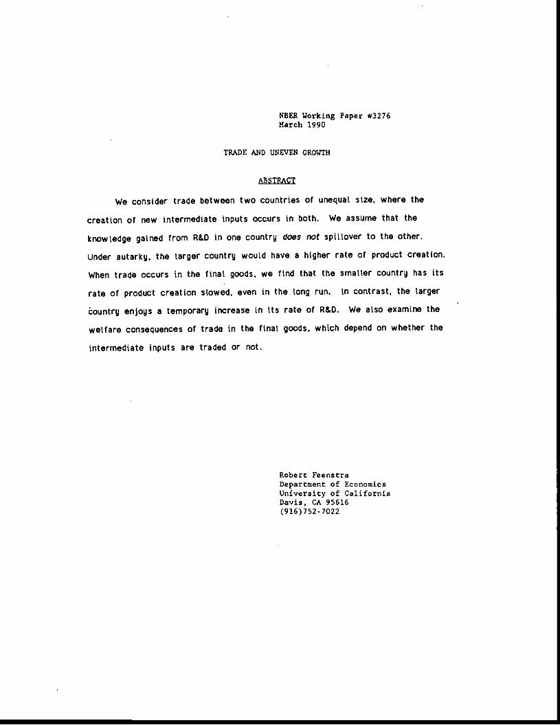
NBER Working Paper #3276March 1990

TRADE AND UNEVEN GROWTH

ABSTRACT

We consider trade between two countries of unequal size, where the

creation of new intermediate inputs occurs in both. We assume that the

knowledge gained from R&D in one country does not spillover to the other.

Under autarky. the larger country would have a higher rate of product creation.

When trade occurs in the final goods, we find that the smalLer country has its

rate of product creation stowed, even in the long run. In contrast, the larger

êountry enjogs a temporary increase in its rate of R&D. We also examine the

welfare consequences of trade in the final goods, which depend on whether the

intermediate inputs are traded or not.

Robert FeenstraDepartment of EconomicsUniversity of CaliforniaDavis, CA 95616

(916)752-7022

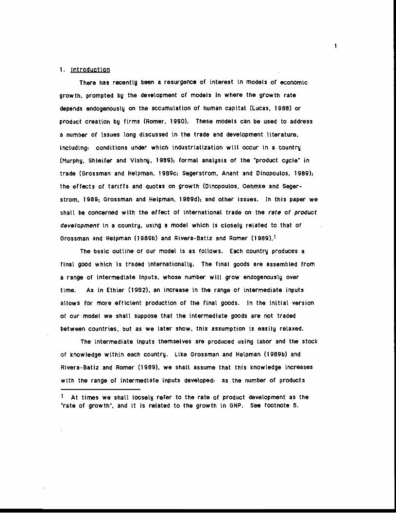
1. Introduction

There has recently been a resurgence of interest in models of economic

growth, prompted by the development of models In where the growth rate

depends endogenously on the accumulation of human capital (Lucas, 1986) or

product creation bg firms (Romer. 1990). These models can be used to address

a number of issues long discussed in the trade and development literature,

including: conditions under which industrialization will occur in a country

(Murphy. Shleifer and Vlshny. 1969); formal analysis of the product Cycle' in

trade (Grossman and Helpman. I 989c: Segerstrom. Anant and Dinopoulos. 1 969);

the effects of tariffs and quotas on growth (Dinopoulos, Oehmke and Seger-

strom. 1989; Grossman and Helpman, 1 gegd): and other issues. In this paper we

shalt be concerned with the effect of international trade on the rate of product

development in a country, using a model which is closely related to that of

Grossman and Helpman (1989b) and Rivera-Datiz and Romer (1969).1

The basic outline of our model is as follows. Each country produces a

final good which is traded internationally. The final goods are assembled from

a range of intermediate inputs, whose number wilt grow endogenously over

time. As in Ethier (1982). an increase in the range of intermediate inputs

allows for more efficient production of the final goods. In the initial version

of our model we shall suppose that the intermediate goods are not traded

between countries, but as we later show, this assumption is easily relaxed.

The intermediate inputs themselves are produced using labor and the stock

of knowledge within each country. Like Grossman and Helpman (1989b) and

Rivera-Batiz and Romer (1989). we shall assume that this knowledge increases

with the range of intermediate inputs developed; as the number of products

1 At times we shalt loosely refer to the rate of product development as therate of growth. and it is related to the growth in GNP. See footnote 6.

grows the fixed costs or creating new ones falls, which will allow continuous

growth to occur. However. unlike these authors, we shalt assume that the

knowledge does not cr033 borders, but is only available to the firms within each

country. This assumption wilt be the driving force behind our results.

Our assumption that knowledge of production techniques does not cross

borders can be justified on several grounds. First, the same assumption is used

in the Alcardian model of international trade, where production functions difrer

internationally. This assumption was dropped in the Heckscher-ohlin model.

where we instead assume identical technologies in all countries. But since

Mlnhas (1962). the empirical evidence has often rejected this assumption. The

most recent, comprehensive test of the Heckscher—Ohlin model Is by Bowen.

Leamer and Sveikauskts (1987). who rind that the predictions of this model fail

sadly, with evidence that technological differences across countries account for

part of the failure.2

Second. our model generates the realistic result that countries will growat different rates. This observation is actually one or the stylized facts put

rorth by Kaldor (1951), and is supported by more recent evidence.3 Even on

purely methodological grounds, we would argue that the analysis of a model

with uneven growth rates across countries in of interest. Much of the existing

literature on endogenous growth has focused on the case where a steady state or

'balanced growth' solution exists, with both countries growing at the same

2 See also the supporting evidence of Dollar, Wolff and Baumol (1988). It isstilt possible that technical knowledge does cross borders, but it used tooslowly to give rise to identical production functions. We discuss the stowtransmission of knowledge in section 6.3 Baumol (1986) has suggested that there is a convergence or growth ratesamong industrial countries, but this evidence is questioned on sample selectiongrounds by Romer (1989). from whom the reference to Kaldor (1961) is drawn.

2

exponential rate. This case naturally simplifies the analysts, but is not

necessarily the most realistic. In our model, no such balanced growth solution

will exist (unless the countries are identical).

To describe our most important resuts. let us measure labor force of

each country in terms of efficiency units in the R&D activity, i.e. the number

of new intermediate inputs which could be developed by the population in a

given year. Then when trade is opened between countries of different size, we

shall find that the smaller country has its growth rate of new products

permanently slowed: even in the long run, this growth rate does not approach

its autarky value. In contrast, the larger country enjoys a higher rate of

product creation, while approaching its autarky rate in the long run. From a

welfare perspective, the effect or these results depends on whether the

intermediate inputs are traded or not.

Several other papers are related to the issues addressed here. Boldrtn

and Scheinkman (1988). Krugman (1988). Lucas (1988) and Young (1989) all

analyse models where trade may be detrimental to growth in a country. These

papers rely on some form of learning by doing, where the technology in each

industry is affected by past production in that, and possibly other, industries.

While our model of endogenous product development is quite different in detail.

the results are remarkably similar to those of Young (1989). A numerical

analysis of trade and product development is provided by Markusen (1989). and

the analysis of this paper was in fact prompted by the desire to obtain

analytical solutions to the questions he posed.4

In the next section we describe our model and determine the equilibrium

conditions. in section 3 we show how these conditions can be reduced to

4 tlarkusen was primarily concerned with determining whether trade wouldeliminate R&D in one country, as we discuss briefly in section 4.

3

certain second-order differential equations. We argue that there is a stable

solution, which describes the equilibrium of the economies. In section 4, the

rates of product development are characterized, with special attention to their

limiting values. In section 5 we provide the welfare analysis. Section 6

discusses generalizations of the model and gives conclusions.

2. The Model

The model we shall use is a simplified version of Grossman and I4elpman

(1989b). so our presentation wilt be brief. There are two countries, labelled

by L:1,2, with labor as the only resource. Let nl denote the number (measure)

or intermediate inputs available in country i at time t, where we suppress t as

an explicit argument. We shall initially suppose that the intermediate inputs

are not traded, so each country uses only its own varieties: this assumption

will be relaxed in section 6. Denote the quantity of each intermediate input by

xi(0), where u is an index or varieties. By symmetry of our model. x(o) will

be constant across all varieties in each country, so that xi(Co) • Xi. Letting j

denote the output or the final good in each country, the production function for

the final goods are given by:

e '1/s 1/atr J X1 d(oI n1 x4, O<&<1. (1)0 )

where the elasticity of substitution among the intermediate inputs is 11(1—01).

Let Pyi denote the price of the final good produced in country i. and Pxi

denote the price of each intermediate input available there. An important

variable in our analysis will be the share of world expenditure spent on the

products of country i. We wilt let i denote the share of world expenditure on

4

fina' products from country i. si • PyIul/(Pyiwi + Py2U2)• Because each final

product is produced with only the intermediate inputs of that country, the value

of output pyy equals the cost of inputs where Xj • njxj denotes the

aggregate quantity of intermediate inputs in country i. It follows that the

share of world expenditure on final products is equal to the share on interme-

diate inputs. s = xXt/(pxX . px2X2). We will use this result frequently.

The final goods y enter the utility functions of consumers, while the

number of intermediate inputs created each period is determined by the R&D

activities of firms. We specify next the problems solved by consumers (section

2.1) and firms (section 2.2). from which the equilibrium conditions for the

economies can be determined.

2.1. Consumers

Consumers in both countries have the identical utility function,

J e(tU log(u(y1(t),y2(v))] dt (2)

where y(t) is the chosen consumption of the final good from country i at time

t. irl.2. We shall suppose that the instantaneous utility function u(y1.g2)

takes on a CES form,

u(y1.y2) (y1 . y1 . 0 c 1. (3)

where the elasticity of substitution is 11(14). Results for I can be

obtained as a limiting case of our analysis. We ignore s 0. however, since in

that case zero consumption of either final good would give utility of -oo in (2).

so that neither country could survive in autarky.

S

Since u(y1.y,) is homogeneous or degree one, the corresponding expenditure

runction can be written as E fl(py,.Py2)u. where it can be thought of as a cost

or living index (it is formally the unit—cost function for (3)). It follows that

utility can be expressed as u E/lt(pyi.py2). or expenditure deflated by the cost

of living index. Substituting this into (2). we can write utility as.

- p( v - t)Ut J e (logE(t) — logit(py1,py2)3 dt . (4)

Consumers maximize (4) subject to a budget constraint stating that the

present discounted value of expenditure cannot exceed the present discounted

value of labor income plus initial assets. We shall suppose that consumers race

an integrated world capital market, so there is a single. endogeflous interest

rate at which citizens of either country can borrow or lend. We will let RU)

denote the cumulative interest factor from time 0 to t (R(0) 1). so that A(t)

is the instantaneous interest rate at time t. Then the first order condition for

maximizing (4) is,

E/E: A-p. (5)

Thus, the path of expenditure will be rising (falling) as the interest rate is

greater (less) than the consumers' discount rate. Savings takes the form of

riskless equities issued by firms to rinance their R&D activities, as we

describe next.

2.2. Firms

Grossman and l4elpman (1989b) and Rivera-Batiz and Romer (1969) assume

that the technical knowledge available in the world is directly related to the

6

product development which has occurred in both countries. In contrast, we

shall assume that this knowledge does not cross borders. Letting technical

knowledge be denoted by Kj. kl .2. we shall assume that this knowledge

increases in proportion to the number of products already developed in each

country, so that Kj u n. This formulation presumes that there are no dimi-

nishing returns in the accumulation of knowledge, and will allow continuous

growth to occur.

The labor cost of developing a new product in each country is given by

ani/Ki • ani/ni. It will be convenient to measure labor in each country in

terms of efficiency units in R&D, so that ant • 1. 1:1 .2. The cost of creating a

new intermediate input is then simply 1 /nj. Firms finance this R&D expen-

diture by issuing equities, which provide a share of the future stream of

profits as a return.

Let the cost or producing each unit or the intermediate input be wiaxi,

where w denotes the wage in country 1:1 .2. The demand for intermediate

inputs is derived from the CES production function in (1). The producers of the

intermediates in each country engage in monopolistic competition, so the prices

Pxi will be a constant markup over marginal costs:-

Pxi = wiaxi/oc . 1:1,2. (6)

It follows that the instantaneous profits from producing the interme-

diate input are (pxl—wtaxl)x( : ((1 -s)/odwiaxixi/ni. where we earlier let X •

nixI denote the aggregate supply of intermediates in each country. At each

instant of time, the development or new intermediate inputs will occur until

the present discounted value of profits is zero, that S:

7

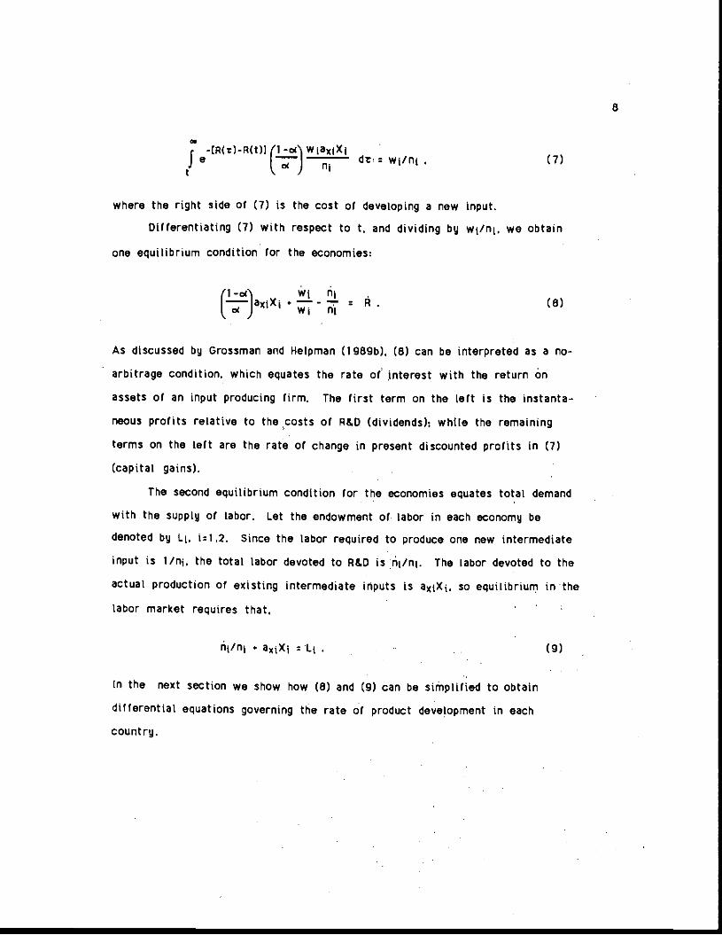
-(R(t)-R(t)] (1 -cC\ wiatXjJ B dy: Wj/flj . (7)

where the right side of (7) is the cost or developing a new input.

Differentiating (7) with respect to t, and dividing b w/fl. we obtain

one equilibrium condition for the economies;

(1-cO Wi ftI—IaiXt •——r : R . (8)wj ft

As discussed by Grossman and Helpman (198gb). (8) can be interpreted as a no-

arbitrage condition, which equates the rate of Anterest with the return an

assets of an input producing firm. The First term on the left is the instanta-

neous profits relative to the costs or R&D (dividends); white the remaining

terms on the left are the rate of change in present discounted profits in (7)

(capital gains).

The second equilibrium condition for the economies equates total demand

with the supply of labor. Let the endowment of labor in each economy be

denoted by Lj. i:1.2. Since the labor required to produce one new intermediate

input is 1/ni. the total labor devoted to R&D is nj/nt. The labor devoted to the

actual production of existing intermediate inputs is aiX,. so equilibrium in the

labor market requires that.

ni/ni • axixi L .

In the next section we show how (6) and (9) can be sirhplified to obtain

differential equations governing the rate of product deve!opment in each

country.

6

3. Ecuations or Motion

To simplify the equilibrium conditions. let p • nj/nj denote the rate of

product development In each country. We can solve For X1 (Li - pi)/axl from

(9). and substitute into (6) obtaining a single equation for each country:

(1—oOLj + c(j/wj) - . (10)

Equation (10) is particularly useful in understanding the Factors governing

long-run growth. Suppose that each country is in aLatarky. and set wj • 1 by

choice of numeraire so that wj 0. Consider a steady-state growth path where

expenditure is constant, so From (5). the instantaneous interest rate A equals

the discount rate p. Then it follows Irom (10) that the long-run growth rate

in each country is:

m g • (1-cOLt — sp >0, (11)

where we assume that this expression is positive. We shall refer to (11) as

the autarky growth rates of the countries, denoted by 9i5 The larger country.

as measured by the effective labor force L. then grows faster in autarky.6

This reflects the tact the the larger country will have a greater variety of

intermediate inputs, more knowledge, and thus lower costs of R&D.

We shalt assume that the two countries are of different size, and let

country 1 be larger in terms of the effective labor force. In autarky, then,

In fact, it can be argued that the autarky economy must jump immediately tothe growth rate 9i• For a single country, the term /5j is zero in (14), and by

inspection the only stable solution is pi g for all t. As discussed below (14).

the unstable solutions with jat-.L or ji-.O are not equilibria.

(1-cOld6 Using (1) and (g), ftnal output yj can be written as n1 (Lt—pt)/at. Then

in autarky, Final output grows at the rate (1—cOgj/d.

g

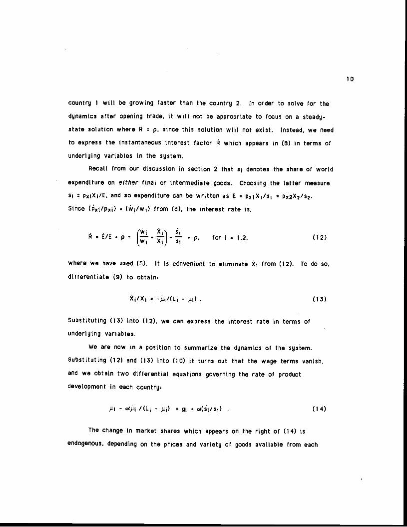
country 1 wilL be growing faster than the country 2. In order to solve for the

dynamics after opening trade, it wiLl not be appropriate to locus on a steady-

state solution where A p. since this solution will not exist. Instead, we need

to express the instantaneous interest factor A which appears in (a) in terms of

underlying variables in the system.

Recall from our discussion in section 2 that sj denotes the share of world

expenditure on either final or intermediate goods. Choosing the latter measure

piX/E. and so expenditure can be written as E Pxl X1/s1 PX2XZ/52.

Since ($Ipxj) (4i/wi) from (6). the interest rate is.

A = E/E + p: [!1.+ jJ + . for I 1.2. (12)

where we have used (5). It is convenient to eliminate Xj from (12). To do so.

differentiate (9) to obtain:

- p1) . (13)

Substituting (13) into (12). we can express the interest rate in terms of

underlying variables.

We are now in a position to summarize the dynamics of the system.

Substituting (12) and (13) into (10) it turns out that the wage terms vanish.

and we obtain two differential equations governing the rate of product

development in each country:

— /(L - MI) g • o((Sj/Sj) . (14)

The change in market shares which appears on the right of (14) is

endogenous, depending on the prices and variety of goods available from each

10

country. To think about the nature of solutions to (14). however, it is

convenient to think or the market shares as exogenous functions of time (taking

on their solution values, for example), Then (14) is a system of nonautonomous

first-order differential equations in pj rig/nj. or second-order differential

equations in ni. This means that we are free to specify the initial number or

products ni(O) in each country, but also have the initial rates of product

development pt(O) as free parameters.

Why does this system not determine the initial rates of product develop-

ment? It turns out that for many initial values JJi(O) the solutions to (14) are

unstable, implying that either jii-.Li as t-.°°, or that piO in finite time. The

former solution means that nearly all the resources in country i are absorbed in

R&D, with expenditure on final goods approaching zero, Residents of that

country would be accumulating increasing amounts of assets from firms, which

would violate their transversality condition. We therefore rule out solutions

in which Pt Li as equilibria.

The other solution we shall rule out is where pj—0 in both countries in

finite time. Adapting an argument from Grossman and Helpman (1989a), we can

argue that this path would violate the optimality conditions of firms. Note

that if R&D ceased in both countries, then expenditure would be constant

(setting either wage as numeraire). so R:p from (5). Instantaneous profits for

input producing firms are ((1 -cO/odaxiX i/ni ((1 -d)/odLjfnj, since j=O in (9).

Since we have assumed that gj:U1 —s)Li—op]>O. it follows that profits exceed

p/nj. Then the present discounted value of profits (using A:p) exceeds 1/ni.

which is the fixed cost of creating a new input. so this is not anequilibrium.

In the next section we solve the differential equations (14). while ignoring

solutions where either jsLj as t-.oo. or P1.0 in both countries.

11

4. Growth Paths

To analyse the erfects or trade on product development, we proceed in

several steps. First, we shalt solve the differential equations (14). treating

the market shares as exogenous functions or time. Second, we shall determine

the equilibrium path of the market shares. Third, we shall then characterize

the rates or product development in each country.

Recalling that p flj/flj. we can multiply (14) by 1 /oi and directly

integrate to obtain,

1 /cd (gI/od)tn1 (L - pi) cdk s e . (15)

where the k > 0 are arbitrary constants of integration. i:1 .2. Multiply both

sides of (15) by the factor —(1 /cOe1/cd

This allows us to again integrate

both sides rrom 0 to t, obtaining,

1 , -Lit/d 1 lcd —(Li .p)ze ni(Q) — kj Jsj e (15)

0

Using equation (18) we can calculate P1 = r/n. We want to rule out

solutions in which Pl-Li as t-.oo, or where p1—0 in finite time. This is done by

choosing ki as,

/ct —(Lj .p)tn(0) /;s e (17)

0

By differentiating (16), and substituting (17). the resulting rates of product

development are:

Calculating MI from (16). it is not difficult to show other values of K1> 0imply that t approaches Li or zero.

12

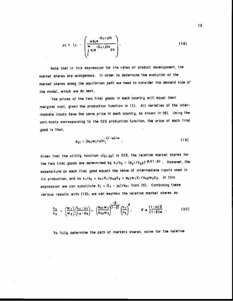
0(510JJi

--(L.p)r

(18)

5s0 drt

Note that in this expression for the rates of product development, the

market shares are endogenous. In order to determine the evolution of the

market shares along the equilbrium path we need to consider the demand side of

the model, which we do next.

The prices of the two final goods in each country will equal their

marginal cost, given the production function in (1). All varieties of the inter-

mediate inputs have the same price in each country, as shown in (6). Using the

unit-costs corresponding to the CES production function, the price of each final

good is then.

—o —o)/dPyi (axjwi/cdn1 . (19)

Given that the utility function u(g1,y2) is CES. the relative market shares for

the two final goods are determined by i'2 (Py1/Py2)"0' . However, the

expenditure on each final good equals the value of intermediate tnputs used in

its production, and so i'2 pxlXI/Px2X2 aX1WIXI/ax2w2X2. In this

expression we can substitute Xi (Lj - J.xj)/axj from (9). combining these

various results with (19), we can express the relative market shares as

s (w (1i -J (axiwi'1-a) (n1' (1 -°$— :111 1:1 I ii. . (20)2 Lw2)l,L21i2) lax2w2) Ln2) (1-$)o

To fully determine the path of markets shares, solve for the relative

13

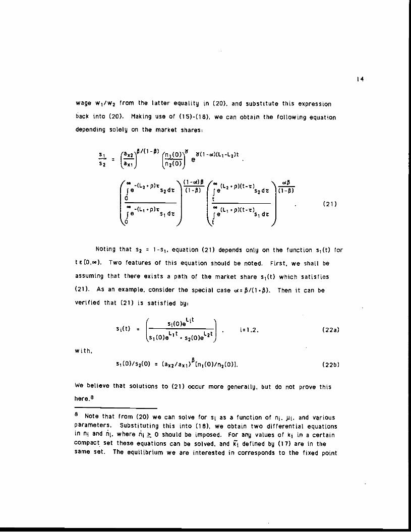
wage w1/w2 from the tatter equality in (20). and substitute this expression

back into (20). Making use of (15)-(18), we can obtain the following equation

depending solely on the market shares:

with.

2 dt (1 -E(l-) JeItI

(1-od)

[—

L2.pXt-t

—(L1 + p)(t-t)p S; dt)t

(22b)

14

Si -tkxi)

(1n1 (0) (i —o(L1 —L2)t

e(n2(o))

(21)

Noting that 2 equation (21) depends only on the function s1(t) for

E C0,oo). Two features of this equation should be noted. First, we shall be

assuming that there exists a path of the market share s1(t) which satisfies

(21). As an example, consider the special case o: /( 1 Then it can be

verified that (21) is satisfied by:

sl(0)elIts(t) = , ir 1,2, (22a)L1t L2tsi(0)e •s2(0)e

51(0)152(0) (ax2Iaxi)[ni(0)fn2(o)),

We believe that solutions to (21) occur more generally, but do not prove this

here.6

Note that from (20) we can solve ror s as a function of ni. p, and variousparameters. Substituting this into (18), we obtain two differential equationsin ni and ni. where iij > 0 should be imposed. For any values of k in a certaincompact set these equations can be solved, and Rj defined by (1 7) are in thesame set. The equilibrium we are interested in corresponds to the fixed point

Second, in our derivation of (21) we have been assuming that >o in

both countries. This means that when the market shares s satisfying (21) are

substituted into (16), we must have pj>0. i:1.2. If instead R&D stops in one

country, then the equations determining the equilibrium are different than what

we have presented. if P2:0. for example, then this is substituted into (20).

and only the formula for Mi is taken from (18). As a result, equation (21)

takes on a somewhat different Form. We will discuss the conditions under

which R&D will stop in one country, after first solving the case where R&D

continues in both.

The general properties of the path of i can be deduced from the fact

that e1 Li11)t appears as fcrcing term in (21). tending to increase the

market share of country 1, This rising market share allows us to determine a

number of results about the long run rates of product development:

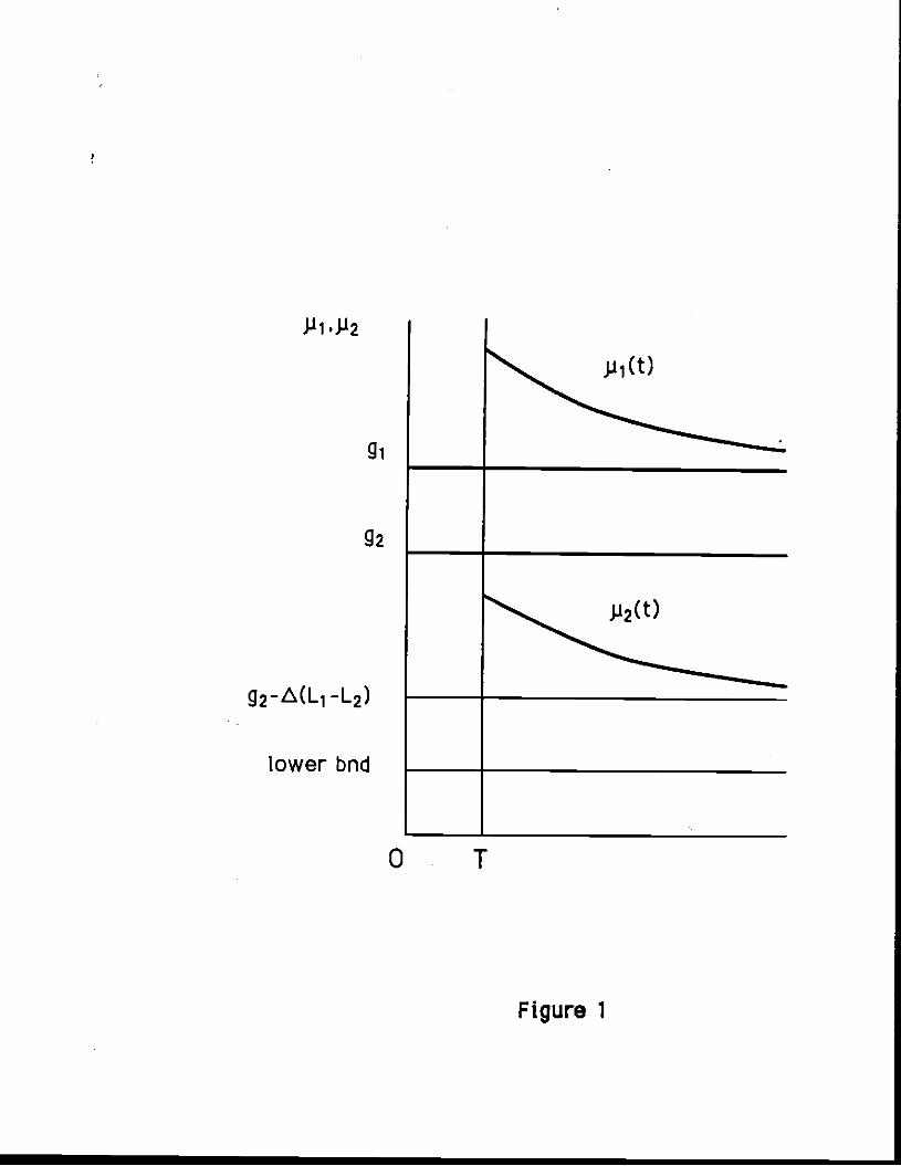
Proposition 1

Suppose that j.Si>O. (:1.2. Then there exists T>O (depending on the parameters

of (21)) such that:llm

(a) i > 0 for t T. and 5i : 1:lim

(b) Mi > g1 for t 1. and Mi

(c) 92 > P2 > g2 - [(1 -o02/o)](L1 - L2) for t T. and

lini . (1oc)2f'(1-fi) 1_iwtthA: L +1]

ki : j. WhiLe it appears that such a fixed point will exist, it is difficult todetermine whether ri1 > 0 or not. If so. then the corresponding path s1(t)

satisfies (21) b.y construction.

15

Referring back to the differential equations (14). we see that the growth

rate jt of an economy is positively related to the change in its market share

i1i Thus, i1 > 0 will tend to quicken product development in country 1.

Since s-.1 then i/si—O. so the positive impact of the rising market share on

growth in country I must be transitory, as indicated in (b). Country 1 wiLl

approach its autarky rate or product development from above. This result is

illustrated in Figure 1, along the path labelled p1(t).

In country 2, which is smaller in terms of the effective labor force, its

falling market share s will slow the rate of product development. Since

it turns out that 2/s2 approaches a strictly negative value. Then the growth

rate in country 2 is permanently less than in autarky, by an amount which

depends on the difference in the labor force of the two countries, as indicated

in Cc). We are not able to determine in general whether J2 approaches its long

run value from above or below. However, notice that when $ r 1 then the lower

bound in Cc) equals the limiting value of P2• In this case P2 must approach its

long run value from above, as illustrated along the path p2(t) in Figure 1.

Note that in drawing Figure 1 we have assumed that the lower bound (or

J2• g2 - [(1 -o2/s)](L1 - L2), is positive. This condition guarantees that growth

will continue in both countries after the opening of trade. As either A grows

or the two country become more different in size, then it becomes less likely

that R&D wilt continue in country 2. Suppose, (or example, that g2 - A(L1 - L2)

< 0. If it also happened that ji2(,O) > 0, then R&D would occur in country 2 for

some finite period of time, and then cease. On the other hand, since we know

from Proposition 1 that p3(O) falls below g2. it is possible that R&D in

country 2 would cease upon the opening of trade.

While the results of Proposition 1 characterize the path of market shares

for large t, we are also interested in determining properties of i for all time.

16

It turns out that s will be monotonically increasing if. either the initialnumber of products in country 2 relative to country 1 is sufficiently small.

ifs lies in the range $/(1+fl sss 0.5. Then we have:

Proposition 2

Suppose that Pi>0. i:1.2, and either:

(I) n2(0)/n1(0) s N (where N>0 depends on the parameters of (21: or,

(ii) $/(1 $) s ss 0.5.Then > 0 for all t0, and the results of Proposition 1 hold for T:O.

Thus, under either conditions Ci) or (ii) we can simply replace T by zer

in Figure 1. and obtain the paths of product development for all t>0. The pr

of Ci) relies an interesting feature of our model. Suppose that instead or

opening trade at time 0. we wait until time T: in the interval (0,T1 we let t

countries grow at their autark rates. Then it turns out that the values of

and Pi for t > T are identical to what they would have been if the countries h

traded during 10.T]. That is. detaing the opening of trade has not effect at

on the rates of R&D or market shares after trade is opened. This means that

for any initial values n(0). irl.2. N can be computed as the ratio n2(T)/n1(T)

the countries grew in autarky over [CT).

Condition (U) was iLlustrated by (22). which is the equilibrium market

shares when 5: $/(1 •$). By inspection, i is increasing for all t in (22). ant

the other results in Proposition 1 then apply for 1:0. The line s:f(1.$)

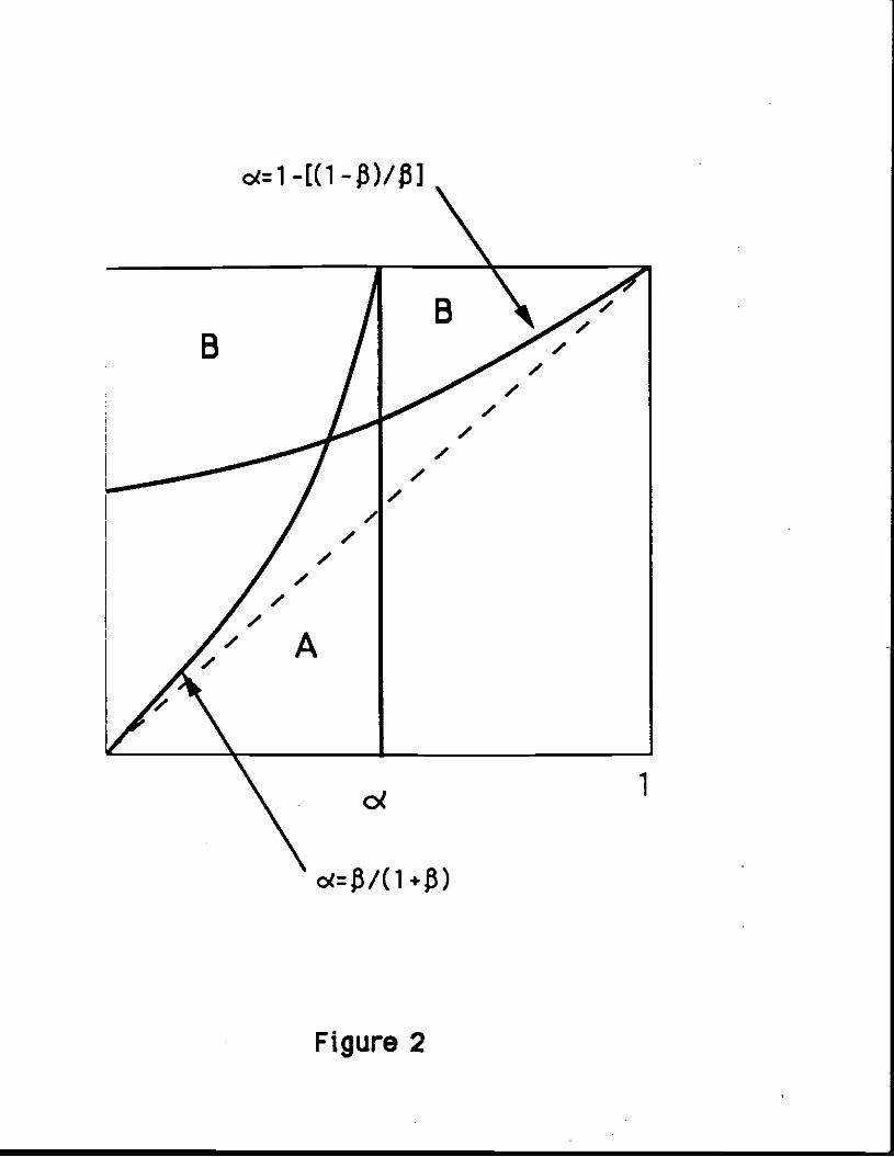
shown in Figure 2. and the region $/(1.$)<sc0.5 is Labelled as A. When

deriving the welfare implications in the next section, we will be supposing

that either (s,$) falls in A, or n2(0)1n1(0) s N. so that Proposition 2 applies

Welf are

Could the slower rate or product development in the small country, as

npared to autarky. ever lead to welfare losses due to trade? To address this

stion. observe that for the utility function in (4) there are two sources of

ns (or loss) from trade: intertemporal gains, by choosing a path or expen-

ure Ej which differs from autarky due to the global capital market: and

:raternporal or statiC gains, by having prices for final goods which differ

m autarky. In this paper we will not attempt to quantify the magnitude of

tertemporal gains.9 instead, we will focus on the intratemporal gains or

sses. by simply comparing the prices faced by each country under free trade

th their values if the economies had continued in autarky. We shall assume

at the results of Proposition 1 apply with T:0.

Prices for final goods affect utility through the price index J'C(pyi .Py2)•

reduction in the price of each final good indicates a fall in the price index Yr.

'4 a rise in instantaneous utility. We need to determine whether the opening

trade leads to such a fail in final goods prices for each country, or not.

First consider country 1. Choosing w1 1 as the numeraire. the prices of

nal goods are given by (1 g). From Proposition 1 we know that this country

periences a higher rate of product development with trade than in autarky. It

'Ilows immediately that Pyi with trade is less than in autarky. and so the

)untry experiences gains even in the consumption of its own final good. In

Idition, country 1 has available the final good from country 2. and so we

)nclude that the price index Tt(pyi 'Py2) must be lower under free trade than in

White we normally think or countries as gaining from intertemporal trade.e do not assert that this result holds here. The difficulty is that the

iterest rate R with trade differs from autarky. so that consumers with

sitive assets may not be able to earn the same interest as in autarky.

18

autarky.

Turning to country 2. we now choose w2 • 1 as the numeraire. Since

rate of product development with trade is less than in autarky, it rotlows

(19) that the price or its own final good y2 is higher under rree trade. Onother hand, country 2 has available the final good from country 1. So wheth

the overall price index Tt(py1,py2) is greater or less than in autarky depends

if the availability of y, more than offsets the higher price or U� In order

make this comparison, we shall use the result:

(1-)/lt(Py,.Py2) Py2 2 ' (2

which is proved in Feenstra (1990). Thus, the price index it with trade will

Lower the smaller is indicating that imports from country 1 make up a

greater portion of country 2 expenditure, or the lower is , indicating that

two final goods are less perfect substitutes.

Let the price or y2 under autarky be denoted by Py2. with the number o

products denoted 112. The relationship between these is shown by (19), where

we set w2 a 1. We are then interested in comparing TUpyi.py3) with

Making use of (23). we see that the price index with trade will be less than

autarky if and only if,

— (1-o)/oC (n2/n2) . (2'

Taking logs of (24). we can express this inequality in the equivalent form:

(1-fl (1—o[lo9(n2/'2fl (2s [ 10952 j'

Consider taking the limit of (25) as t.. Applying L'Hospitals Rule,

ression in square brackets on the right becomes .. (.' - g2)(2's2) : 6.

ig (14) and the tact that P2 • 0. Thus, as t.". the inequaLity (25) becomes

5)/$J1-cO. which is certainly violated for some values of and 5. We

dude that for these values of 6 and , there will exist I such for t>T, the

:e index (pyi.Pyz) with trade exceeds the price Py2 raced in autarky.

These results are illustrated in Figure 2. In the upper portion of this

gram we show the region (1 -5)15 <(1 -oO, labelled as B. in which (25) is

Lated and the price index for country 2 exceeds its autarky value for

ficiently high t. As an extreme example, consider 5: 1. so that the final

ds of each country are perrect substitutes. Then the slower rate or product

'elopment in country 2 with trade will lead to a higher price for Y2. and this

not offset by the availability of Ui (since this perfect substitute does not

wide extra utility). In this extreme case the price index 7t(pyi .Py2) with

de exceeds the autarky price 'y2 for all t after trade is opened. For lower

ues of 5. the price index for country 2 will be higher than in autarky only

a restricted range or , and for t sufficiently high.

Next, consider the complementary region in Figure 2. in which (1 -5)15

ct). Can we conclude that the prices index for country 2 will be less than in

:arky. so that the country experiences gains from trade in this sense? It

ns out that this assertion is true so long as a condition on the initial value

s2 is satisfied. Our welfare results are summarized by:

position 3

pose Proposition 1 applies with T :0. Then:

With w1 • 1. the price index of country 1 under free trade is less than it

uld have been in autarky;

20

(b) With w2 1. and < 1-Ri —$)/fl, there wilt exist T such that for t>r t

price index for country 2 under trade exceeds its autarky value;

(c) With w2 • 1. and 1 -[(1 -fl/$1. the price index for country 2 will be 1€

than in autarky provided that,

. p52(0) + p • ((1 -)/]2(L1 -L2)J ' (2!

It is difficult to check whether (25) is satisfied in general, since the

initial market shares are determined by (21). However, lower values of the

initial products n2(0)/n1(O) in (21) tend to correspond to lower values or th

initial shares 52(0)151(0), as shown by the example in (22). So condition (2

is consistent with condition (i) or Proposition 2 that n2(0)/n1(0) SN, and tl

is one of the conditions that allows us to apply Proposition 1 with T :0.

We conclude this section by briefly examining the behavior of relative

wages in the countries. From (20) we obtain,

(axjwi'1 (i.s'l -$)i (flL'f1°'°, (V

ax2w2) 52) Ln2)

Differentiating this expression and making use of earlier results, we can shc

that if i, > 0 for t T. then (w2/w,) will be declining for t T.1 This

behaviour of the relative wage is in constrast to the relative product price:

when s1 > 0 then the terms of trade (Py2Py1) must be increasing, leading to

the toss of market share for country 2. Thus, our model generates opposite

movements in the relative wage and terms of trade across countries.

10 We use (A3) and (A6) from the Appendix.

)eneralizatiOfl and Conclusions

We have been assuming throughout the paper that the intermediate inputs

not traded internationally, but can now relax this. When these products are

ad the final goods in (1) will use the inputs From both countries, so that y

g2 will have identical prices and sell in identical quantity.1 1 It follows

the market shares For the final goods are Fixed at 1/2. Since y1 Y2 the

antaneous utility function in (3) can be written as.

$ $1,1uCy1,y2) (y1 + y21

1/s l ci n2 1/c(2 5 x1 dC.) • 5 x2 dco , (3')

0 0

•re the second line follows from ui Y2 in (1), wtth the intermediate inputs

nd x2 from both countries used in the production of each final good. Corn-

rig (31 with (3). we see that the utility function with intermediate inputs

led is identical to our earlier case with ci: imposed there. Working

)ugh the rest of our earlier analysis, we find that it continues to hold, with

nterpreted as the share of world expenditure on intermediate inputs oF

itry i. We conclude that the model with free trade in the intermediate

its is formally equivalent to the case of no trade with c$ imposed.

Thus, the qualitative results on growth rates reported in Propositions 1

2 carry over to the case of free trade in the intermediate inputs. The

rare results in Proposition 3 also carry over, but now the condition that

$ makes a dIfference. In Figure 2. the restriction cn$ corresponds to the

This result depends on having the final goods costlessly assembled from thetrmediate inputs, so that that wage tn each country does not affect the finald's price,

22

diagonal line, which lies outside the region B where country 2 couLd face a

possible welfare loss. Thus, when intermediates are traded, and condition (2

is satisfied, we conclude that country 2 wilt face lower prices with trade a

experience gains in this sense. The reason is that the slower rate or produci

development there is offset by the availability or imported intermediates, s

that the final goods price Py2 is less than in autarky.

Our result that the possibility of a welfare loss for country 2 occurs

mainly in the absence or trade in the intermediate inputs is consistent with

the literature on trade and distortions (Bhagwati. 1983). in this case, openi

trade in the final goods can worsen the distortion caused by no trade in the

intermediates, leading to the possibility of a higher price index in country 2

with trade. From a policy perspective, our results indicate the importance r

free trade in intermediate products.

Two other generalizations can be readily discussed. First, suppose tha

the knowledge in one country does spiltover to the other, but at a slow rate.

Grossman and Helpman (lgegb) examine the case where knowledge disseminat

within and across countries with exponential lags. In order for a balanced

growth solution with both countries growing at the same rate to exist, they

argue that the lags within and across countries should be similar. We have

considered the extreme case or instantaneous dissemination within a country

but zero spiltover across countries, so that the nations grow at uneven rates

Their discussion suggests that a similar result might be obtained with limi

but small. spilLover of knowledge across countries.

Second. suppose that a country can either create new products, or imit

the technology of the other country (at some fixed cost). This approach is

taken by Grossman and Helpman (1 989c). Significantly, they assume that th

technical knowledge in the smaller country (the South) depends only on the

ovation and imitation which has occurred there, so that there is no direct

hover of knowledge from the Larger country (the North). While this is the

ie assumption we have made, they obtain the quite different result that both

ntries can grow at a quicker rate with trade than in autarky. However, this

utt depends on the South being not too small: it must have enough resources

imitate at the same rate as Northern innovation.1 2 For smaller Southern

intries, the balanced growth equilibrium they have described does not occur.

would conjecture that in this case the countries will grow at uneven rates.

we have analysed here.

In their Figure 1. SS cannot lie below NN.

24

ADDendix

Proof of Proposition 1

We first solve for the limiting values of s and J.lj, and then determine thei

values for large t in part Cd).

I.!1 For any 0<0<1. we need to show that there exists I such that s1(t)>

for t >1. Suppose not. Then for some Ocaci, we must have either s1(t) <a

t>T,, or s1(tØ:o for an increasing, unbounded sequence of times tj:t1,t2,t3,..

In the former case we can take the limit of (21) as t.. and find that the

side is less than 01(1-0) but the right side approaches infinity, which is a

contradiction. So consider the latter case.

Evaluating (21) at the times t1. •we see that the left side is constant

s1(tj)/s2(tj) : o/(1 -0). The term et(1_ t)2 iLOti on the right approaches

infinity as t-.oo. so the bracketed expression on the far right of (21) must

approach zero. It follows that,

lim7

p)(t1—t) dt 0 . (A

Since s2(tj) :0 in the numerator of (18). it follows that p2(tj) must becom

negative for large t. This contradicts our assumption that pj>0. i:1.2. II

follows that no such sequence exists, which proves that s-.1.

I Using L'Hospitals flute, take the limit of (16) to obtain

Urn tim (Sfl: gj • s .

tim lAm . timFor i1 . : 1 implies that t— i : 0, so that : g1.

urn 2For i:2, we need to evaluate (—') and then apply (A2). Differen-

ting the tog of (21) and making use or (18). we can show that,

l2 12 (L1-L2) - (c1)1-2 . (A3)

trig our results in (a) and (b), it follows that,

r (i-#r)(i - .t $2) - aLI-L2)

mbining (A4) with (A2) for i:2, the Limiting value of $2 can be computed.

Substituting the limit of j.22 back into (A4). we obtain,

: () - (.i±)2 [!.L±. lf'L1-L2) C 0 . (As)

ice (As) is less than zero, it follows that there exists T (depending on the

rarneters or (21)). such that 2<° and >0 ror t>T. To derive the

)perties of i for tT, integrating b parts to obtain the formula,

JSj e +P)?dt(Lj.p11 [sieL1t ile_a1ttdt]

bstituting this into the numerator or (18). we can write the rates or product

velopmeflt as.

- ( -(L.p)z -(Ljtp)r '\.i(: iClisle dt/jsje dtl. (A6)t )

en >0 for all t>T implies that p > g, and $2 < g2. To compute the lower

und on $2. use s>O in (AS) to obtain:

26

P2 > Mi - (1)L1 -L2) > - (Li -1.2) g2 -(1

(L; —1.2)

Proof of ProDosition 2

Once we establish that >0 for t>0. it is immediate from our discussion

just above in (d) that Proposition 1 applies for T0.

(fl For any value of n2(O)/n1(0). and other parameters of (21). let s1(t)

denote the market shares and T denote the time at which i > C for t > T.

Then define N . (n2(O)/ni(O)l 24I)T Consider the new starting values

n2(O)/n1C0) N. and let the resulting market shares be denoted by j(t). Then

by inspection we see that (t) • s(t.T) will satisfy (21). Since >0 for

> T. it follows - 11>0 for t0. By the same logic, this result will hold fot

all initial values n2(0)/n1(0) I N.

Ufl We will assume that fl/I] .$) < ot S 0.5. and deal with $10 $) in th

text. Note that these inequalities on ot imply.

1-ac 2 1(1-fl) -I-i $(1-2u)(ci) 1i

> sci-a 0 (Al)

Urn i 1-O( 2 (1-fl) -1Suppose that s1(t0):0. From (A5). .. (n) (—;—) [ cifi • i] (L1-L2). so

using (Al) there must exist t1 t0 such that,

(42) $('c (L1L2) at t1. (A8)

Then substituting this into (A3). we obtain (p -p2) (L1 —L2) at t1. The

differential equations (14) can then be written as.

(L-p)-

(L2-p2)(P1-i2) - (g1-g2) - cl/S152)

(L1-L2)(s(i.$)-$1 > . (Ag)

-e the second tine follows using (p1-ja2) (L1-l.2). (AS) and s> $I(l 4).

Since (L1-p1) (L2-ji2) at t1, it is evident from (A9) that (A1—ü2) > 0

Taking the derivative of (A3). it follows that for t slightly greater

t1 we must have (1/$12) less than ($(l -2s)/s(l -$))(L1-L2). However.

implies that (1/l2) can never exceed ($(l -2s)Is(l-$)](Li-L2), since

never it reaches this value (from below) it then becomes less. But this

:radicts that fact that (Isi s2) > ($(l -25)104(1 -$)J(L1 -L2) from (Al).

allows that s1(t0):O cannot occur, and since s.1. then >0 ror all t.0.

DI of ProDositton 3

and (b) These are proved in the text.

Note that s . 1 —Ui 4)/$I implies s 1 Is. since r (1 -cO$I(1 -$)s.

n (n2I2) > (n2/A)1 "° . We wilt show that.

(n2I)1 > (s21s2(0)J (L2 + . ((i-;)/od2(L, -L2))(Ala)

using (26) this implies (n2/R2) (fl22)1 " > 2. which proves (24).

To establish CAb), use (15) and (17) to write.

IsC(L2_J12)Js2eO2dtiIss2 . (All)

ce s1 >0 for alt t. then P2 > g — UI -s)21s)1(Li —L2) from Proposition 1(c).

I it follows that (L2—j.a2) < s(L2.p) . ((1 —o02/s)](L1—L2). Substitute this

a (All), and use 52(0) > s to replace 2 in the integral. Then evaluating the

egral. we obtain (Ala).

26

References

Bhagwati. Jagdish N. (1983) 'The Generalized Theory of Distortions andWelfare,' in Essaus in International Economic Theoru, vol. 1. CambridgcMIT Press. 73-94.

Baurnol. William J. (1986) 'Productivity Growth. Convergence, and WelfareWhat the Long-Run Data Show,' American Economic Review 76, 1072-1 at

Boldrin. Michele and Jose A. Scheinkman (1989) 'Learning-By-Doing. International Trade and Growth; A Note,' in Philip W. Anderson, Kenneth J. Arand David Pines, eds. The Economu as an Evolving ComDlex Sustern. NewYork; Addison-Wesley. 265-300.

Bowen, Harry P.. Edward E. Learner and Leo Svetkauskas (1967) MulticountrMultifactor Tests of the Factor Abundance Theory.' American EconomicReview 77. 791 -809.

Dinopoulos. Elias. James F. Oehmke and Paul S. Segerstrorn (1989) 'High-• Technology-industry Trade and Commercial Policy.' Michigan State Univ

mirneo.

Dollar, David. Edward N. Wolff and William J. Baumol (1968) 'The Factor_EEqualization Model and Industry Labor Productivity: An Empirical Test PCountries.' in Robert C, Feenstra, ed. EmDirical Methods for InterriatloTrade. Cambridge: MIT Press, 23-47.

Ethier. Wilfred (1962) 'National and International Returns to Scale in theModern Theory of International Trade.' American Economic Review 72, 3405.

Feenstra, Robert C. (1990) 'New Goods and Index Numbers: Explaining the Cin U.S. Imports.' Univ. of California. Davis. in process.

Grossman. Gene H. and Elhanan Helpman (1 989a) 'Product Development andInternational Trade,' Journal of Political Economu 91. 1261-1283.

Grossman. Gene H. and Elhanan Helpman (1 989b) 'Comparative Advantage anLong-Run Growth.' HOER Working Paper no. 2809. American Economic Reforthcoming.

Grossman. Gene M. and Ethanan Helpman (1969c) 'Endogenous Product Cycte

3ER Working Paper no. 2913.

;man. Gene H. and Elhanan Helpman (1989d) Growth and Welfare in a Smallen Economy.' NBER Working Paper no. 2970. in Elhanari Helpman and Assafizin. eds. International Trade and Trade Policu, MIT Press, forthcoming.

r. N. (1960 Tapital Accumulation and Long Run Growth,' in F.A. Lutz andC. Hague. eds.. The TheQru of Capital. New York; St. Martins Press, 177-22.

nan. Paul (1988) 'The Narrow Moving Band, the Dutch Disease, and thensequences of Mrs. Thatcher,' Journal of Development Economics 8. 149—

31.

;. Robert E. (1988) 'On the Mechanics or Economic Development.' Journal oronetaru Economics 22. 3-42.

.isen, James A. (1989) 'First Mover Advantage, Blockaded Entry, and the:onomics of Uneven Development,' in Elhanan Helpman and Assal Razin, eds.'ternational Trade and Trade Policu, MIT Press, forthcoming.

is, B.S. (1962) 'The Homohypallagic Production Function. Factor—Intensityversals and the Heckscher-Qhlin Theorem.' Journal of Political Economu

3, 138-156.

.1g. Kevin M.. Andrei Shleifer and Robert Vishny (1989) 'Industrializationd the Big Push,' Journal of Political Economu 97, 1003-1026.

-a-Batiz, Luis A. and Paul H. Romer (1989) 'International Trade Withidogenous Technical Change,' University or Chicago. mimeo.

'r, Paul H. (1989) 'Capital Accumulation in the Theory of Long Run Growth.'I Robert J. Barro, ed. Modern Business Cucle Theoru. Cambridge; Harvardniversity Press, 51—127.

,r, Paul N. (1990) Endogenous Technical Change,' Journal of Political;onomu, forthcoming.

rstrom, Paul S., r.C.A. Anant and Elias Dinopoulos (1989) 'A Schumpeterianodel or the Product Life Cycle.' American Economic Review, forthcoming.

g. Alwyn (1 989) 'Learning By Doing and the Dynamic Gains from Trade,'Lumbia University, mtmeo.

30

P1.J2

g2-ML1 -L2)

lower bnd ______ __________

I

Figure 1

o(:1 -[(1 -16)/fl

Figure 2

o/(1 .+)